automatic authorization analysis - uni-saarland.de · depicted in figure 1.1. when a company...
TRANSCRIPT

Automatic Authorization Analysis
Manuel Lamotte-Schubert
Dissertation zur Erlangung des Gradesdes Doktors der Ingenieurwissenschaften
der Naturwissenschaftlich-Technischen Fakultatender Universitat des Saarlandes
Saarbrucken2015

Day of Colloquium September 18th, 2015Dean Prof. Dr. Markus BlaserChairman Prof. em. Dr. Dr. h.c. Reinhard WilhelmSupervisor and First Reviewer Prof. Dr. Christoph WeidenbachSecond Reviewer Dr. habil. Peter BaumgartnerScientific Assistant Dr. Swen Jakobs
III


Abstract
Today many companies use an ERP (Enterprise Resource Planning) systemsuch as the SAP system to run their daily business ranging from financialissues down to the actual control of a production line. These systems are verycomplex from the view of administration of authorizations and include a highpotential for errors. The administrators need support to verify their decisionson changes in the authorization setup of such systems and also assistance toimplement planned changes error-free.
First-order theorem proving is a reliable and correct method to offer thissupport to administrators at work. But it needs on the one hand a corre-sponding formalization of an SAP ERP system instance in first-order logic,and on the other hand, a sound and terminating calculus that can deal withthe complexity of such systems. Since first-order logic is well-known to beundecidable in general, current research deals with the challenge of findingsuitable and decidable sub-classes of first-order logic which are then usable forthe mapping of such systems.
This thesis presents a (general) new decidable first-order clause class, namedBDI (Bounded Depth Increase), which naturally arose from the requirementto assist administrators at work with real-world authorization structures inthe SAP system and the automatic proof of properties in these systems. Thenew class strictly includes known classes such as PVD. The arity of functionand predicate symbols as well as the shape of atoms is not restricted in BDIas it is for many other classes. Instead the shape of “cycles” in resolutioninferences is restricted such that the depth of generated clauses may increasebut is still finitely bound. This thesis shows that the Hyper-resolution calculusmodulo redundancy elimination terminates on BDI clause sets. Further, itemploys this result to the Ordered Resolution calculus which is also proved toterminate on BDI, and thus yielding a more efficient decision procedure whichis able to solve real-world SAP authorization instances. The test of conditionsof BDI have been implemented into the state-of-the art theorem prover Spassin order to be able to detect decidability for any given problem automatically.The implementation has been applied to the problems of the TPTP Libraryin order to detect potential new decidable problems satisfying the BDI classproperties and further to find non-terminating problems “close” to the BDIclass having only a few clauses which are responsible for the undecidability ofthe problem.
V

Zusammenfassung
Viele Unternehmen verwenden heutzutage ERP (Enterprise Resource Plan-ning) Systeme wie das SAP System zur Unterstutzung des taglichen Geschaftsangefangen vom Rechnungswesen bis hin zur Steuerung einer Fertigungslinie.Diese Systeme sind hinsichtlich der Verwaltung von Berechtigungen sehr kom-plex und besitzen deswegen eine hohe Fehleranfalligkeit. Administratorenbenotigen deswegen sowohl Unterstutzung, um ihre Entscheidungen bei An-derungen im Berechtigungs-Setup zu verifizieren und auch Hilfe, um geplanteAnderungen an Berechtigungen fehlerfrei umsetzen zu konnen.
Theorembeweisen in Pradikatenlogik ist eine zuverlassige und korrekte Meth-ode, um Administratoren die notwendige Unterstutzung bei der Arbeit zu bi-eten. Sie benotigt jedoch auf der einen Seite eine entsprechende Formalisierungeiner SAP ERP System Instanz in Pradikatenlogik, und auf der anderen Seiteeinen korrekten und terminierenden Kalkul der mit der Komplexitat solcherSysteme umgehen kann. Da Pradikatenlogik bekanntlicherweise im Allge-meinen unentscheidbar ist, beschaftigt sich die aktuelle Forschung mit derHerausforderung, geeignete und entscheidbare Teilklassen der Pradikatenlogikzu finden, die dann fur die Abbildung solche Systeme benutzbar sind.
Diese Arbeit stellt eine (allgemeine) neue entscheidbare Klauselklasse inPradikatenlogik mit dem Namen BDI (Bounded Depth Increase) vor, die aufnaturlichem Wege aus der Anforderung zur Unterstutzung der Administra-toren bei der praxisorientierten Arbeit mit Berechtigungsstrukturen im SAPSystem und dem automatischen Nachweis von Eigenschaften in solchen Sys-temen entstand. Die neue Klasse enthalt bereits bekannte Klassen wie PVD.Die Stelligkeit von Funktions- und Pradikatssymbolen wie auch die Gestalt derAtome ist in BDI nicht beschrankt, wie es bei vielen anderen Klassen der Fallist. Stattdessen wird die Gestalt von Zyklen in Resolutionsinferenzen derartbeschrankt, dass die Tiefe von generierten Klauseln zwar ansteigen kann, aberletztendlich begrenzt ist. Diese Arbeit zeigt, dass der Hyperresolutions-Kalkulzusammen mit der Eliminierung von Redundanzen auf BDI Klauselmengenterminiert. Zusatzlich wird das Ergebnis ubertragen auf den Kalkul der geord-neten Resolution, fur die ebenfalls die Terminierung auf BDI bewiesen wirdund damit eine effizientere Enscheidungsprozedur liefert, die fur praxisorien-tierte SAP Instanzen anwendbar ist. Der Test der Bedingungen fur BDIwurden im aktuellen Theorembeweiser Spass implementiert, um die Entschei-dbarkeit fur ein beliebiges Problem automatisch feststellen zu konnen. Die Im-plementierung wurde auf die aktuelle TPTP-Problem-Bibliothek angewendet,um neue entscheidbare Probleme zu finden, die den Anforderungen der BDI
VII

Klasse genugen und weiterhin nicht terminierende “beinahe”-BDI Problemezu ermitteln, bei denen nur wenige Klauseln verantwortlich fur die Unentschei-dbarkeit des Problems sind.
VIII
Acknowledgements
This work would not have been possible without the persistent support andcontinuous motivation of my supervisor Prof. Dr. Christoph Weidenbach. Iwould like to thank him for his scientific guidance, patience and cooperationin all aspects accompanying this thesis. I’m also grateful to Dr. habil. PeterBaumgartner, who invited me for a visit at NICTA Canberra, Australia, whereI spent 4 months doing research on business rules. Furthermore, I would liketo thank my colleagues at the Max Planck Institute for Informatics with whomI often had supporting discussions.
I thank the anonymous reviewers of the publications that are incorporatedin this thesis. Their comments have helped me considerably in obtaining afresh view on some aspects and in improving both the quality of my work andits presentation.
Especially, I would like to thank my wife Agata Schubert and my family whosupported me over the whole time at the Max Planck Institute for Informaticsand encouraged me to finish this thesis.
Finally, I thank the (yet to come) readers of this thesis for their interest inmy work. I sincerely hope that you can benefit from it for your own work.
IX

Contents
1 Introduction 11.1 Motivation . . . . . . . . . . . . . . . . . . . . . . . . . . . . . 1
1.2 Contribution . . . . . . . . . . . . . . . . . . . . . . . . . . . . 4
1.3 Related Work . . . . . . . . . . . . . . . . . . . . . . . . . . . . 6
2 Foundations 92.1 Mathematical Foundations . . . . . . . . . . . . . . . . . . . . . 9
2.2 First-Order Logic . . . . . . . . . . . . . . . . . . . . . . . . . . 10
2.2.1 Syntax . . . . . . . . . . . . . . . . . . . . . . . . . . . . 10
2.2.2 Semantics . . . . . . . . . . . . . . . . . . . . . . . . . . 15
2.3 First-Order Reasoning . . . . . . . . . . . . . . . . . . . . . . . 15
2.3.1 Inferences . . . . . . . . . . . . . . . . . . . . . . . . . . 16
2.3.2 Reductions . . . . . . . . . . . . . . . . . . . . . . . . . 18
2.3.3 Soundness and Completeness . . . . . . . . . . . . . . . 18
2.4 Graphs . . . . . . . . . . . . . . . . . . . . . . . . . . . . . . . . 19
3 The SAP (Authorization) System 213.1 Authorization Checks . . . . . . . . . . . . . . . . . . . . . . . 23
3.1.1 Transactions . . . . . . . . . . . . . . . . . . . . . . . . 23
3.1.2 Authorization Objects . . . . . . . . . . . . . . . . . . . 24
3.1.3 Authorizations . . . . . . . . . . . . . . . . . . . . . . . 24
3.1.4 Authorization Check Procedure . . . . . . . . . . . . . . 26
3.2 The Authorization Setup . . . . . . . . . . . . . . . . . . . . . . 27
3.2.1 Authorization Profiles . . . . . . . . . . . . . . . . . . . 27
3.2.2 Roles . . . . . . . . . . . . . . . . . . . . . . . . . . . . 29
3.3 Business Processes . . . . . . . . . . . . . . . . . . . . . . . . . 32
3.3.1 The Purchase Process . . . . . . . . . . . . . . . . . . . 33
3.4 Business Policies . . . . . . . . . . . . . . . . . . . . . . . . . . 37
4 Formalization of the SAP Authorization Layer 414.1 Abstractions . . . . . . . . . . . . . . . . . . . . . . . . . . . . 41
4.2 Construction . . . . . . . . . . . . . . . . . . . . . . . . . . . . 42
4.2.1 Authorization Setup . . . . . . . . . . . . . . . . . . . . 42
4.2.2 Authorization Checks . . . . . . . . . . . . . . . . . . . 44
4.2.3 Purchase Process . . . . . . . . . . . . . . . . . . . . . . 45
4.2.4 Business Policies . . . . . . . . . . . . . . . . . . . . . . 51
XI
Contents
4.2.5 Purchase Process + Business Policies Reviewed . . . . . 52
5 The Clause Class BDI 555.1 Prerequisites . . . . . . . . . . . . . . . . . . . . . . . . . . . . 565.2 Definition of BDI & Examples . . . . . . . . . . . . . . . . . . 585.3 Termination of Hyper-Resolution on BDI . . . . . . . . . . . . 615.4 From Hyper to Ordered Resolution . . . . . . . . . . . . . . . . 84
6 Implementation 87
7 Solving SAP Authorization Problems with BDI 107
8 Application to the TPTP Library 109
9 Conclusion 113
Bibliography . . . . . . . . . . . . . . . . . . . . . . . . . . . . . . . 115
XII

List of Figures
1.1 Analysis of authorizations in SAP ERP. . . . . . . . . . . . . . 2
2.1 A directed graph. . . . . . . . . . . . . . . . . . . . . . . . . . . 19
3.1 Authorization object structure. . . . . . . . . . . . . . . . . . . 243.2 Authorization (instance of an authorization object). . . . . . . 253.3 Complete picture of SAP authorizations. . . . . . . . . . . . . . 283.4 Structure of a simple authorization profile . . . . . . . . . . . . 293.5 Structure of a composite authorization profile. . . . . . . . . . . 303.6 Structure of a single role. . . . . . . . . . . . . . . . . . . . . . 313.7 Structure of a composite role. . . . . . . . . . . . . . . . . . . . 323.8 Purchase process overview. . . . . . . . . . . . . . . . . . . . . 333.9 Screen to create a requisition. . . . . . . . . . . . . . . . . . . . 343.10 Screen to release a requisition. . . . . . . . . . . . . . . . . . . 363.11 Screen to create an order. . . . . . . . . . . . . . . . . . . . . . 38
4.1 Dependency graph. . . . . . . . . . . . . . . . . . . . . . . . . . 53
5.1 Proof levels ([k + 1], [k] and [k − 1]) regarding current, andparent clauses used in the induction step of Theorem 5.11. . . . 64
XIII


List of Tables
3.1 Authorization values . . . . . . . . . . . . . . . . . . . . . . . . 25
8.1 Problems “close” to the BDI class . . . . . . . . . . . . . . . . 111
XV


1 Introduction
1.1 Motivation
Computer systems have been invented to help people in many areas of every-day life. Especially, there are powerful software systems aiming to supportthe operation of a business. One typical software of this area is called Enter-prise Resource Planning (ERP) system. Typically, ERP systems are built tointegrate almost all facets of the business across a company including areaslike finance, planning, manufacturing, sales, or marketing. The broader thefunctionality of such a system, the larger the number of users, the greaterthe dynamics of a company, the more complex is the administration of theauthorizations. In particular, this applies to the well-known SAP ERP system(formerly known as SAP R/3) offered by SAP SE1.
The typical scenario of a company using an ERP system like SAP ERP isdepicted in Figure 1.1. When a company decides to use a system like SAPERP, it first formulates its business as processes. A typical business processis the purchase process that is used as a case study in this thesis. It startswith the creation of a purchase requisition out of the requirement for an asset,followed by the release of such a requisition, and finally the transformation ofthe released requisition into the purchase that is eventually sent to a supplierwho is then responsible for the delivery of the asset. Very often each step of aprocess corresponds to a particular role of a company employee. For our exam-ple, the transformation of the released requisition into a purchase is a typicalbuyer activity. On the process layer, the company also decides on regulationsand constraints which are typically called business policies. The developmentof processes and the authorization concept is guided by business policies. Forexample, a business policy might require that the activity of creating a requisi-tion and creating a purchase must always be separated, performed by differentpersons, and therefore must not be contained in one authorization role. Thisis a typical rule out of the Segregation/Separation of Duties (SoD) approach.Once the processes and authorization concept are defined, the configurationis implemented into an SAP ERP instance leading to a corresponding processand authorization setup. The authorization setup exactly defines for a userwhether or not he/she is authorized to execute certain functions in the system.
The initial setup of a new SAP system instance typically requires a so-called
1SAP R©, SAP R© R/1 R©, SAP R© R/2 R©, SAP R© R/3 R©, and SAP NetweaverTMare the trade-marks or registered trademarks of SAP SE in Germany and in several other countries.
1

1 Introduction
Processes
AuthorizationConcept
ProcessSetup
Business Policies
Authorization Setup
SAP R/3 Instance
Business
ProcessFormalization
Business PolicyFormalization
Authorization Formalization
First-Order Formal Model
Properties
Company
Figure 1.1: Analysis of authorizations in SAP ERP.
Customizing to meet the business needs of the company. Therefore, two SAPERP implementations as used by two different companies will usually neverlook the same. The Customizing is mostly carried out by separate companieswhose daily business is to configure all the customizing settings, and to setupthe corresponding authorization concept. Correspondingly, these companiesusually have appropriate routines for these tasks which try to ensure that noerrors occur in the initial setup. However, as soon as the system is productive,it requires permanent and individual maintenance. Business policies and pro-cesses are less likely to change and if they change this is not done on a dailybasis but by additional smaller SAP change or introduction projects. However,for example, changes might be necessary because of changes in the organiza-tional structure of the company or the employees change. Such changes result
2
1.1 Motivation
in changes of the authorizations and, because of the complex structure andthe sheer size of most of today’s SAP systems, it is practically impossible toguarantee the compliance of the business policies with the process and au-thorization setup afterwards by hand without the support of rigid tools andprograms. Furthermore, it is non-trivial to set up new authorization roles foremployees following organizational changes in the business without destroyingthe overall compliance between the authorization setup and the business poli-cies. In practice, especially changes to the authorization setup, for example,caused by organizational changes in a company, cause the most headache toSAP authorization administrators. Who has currently access or permission toretrieve or change certain sensitive data? Does the system (still) comply withthe company’s business policies initially and especially after the change? Suchquestions are a daily occurrence for SAP system administrators who have tomanage a vast number of users, roles, and authorizations and it’s not trivialto give correct answers to these critical questions. This is the point whereautomatic tools come into play which support the administrators by verifyingtheir decisions and assisting them to implement planned changes error-free.
A suitable and particularly reliable solution to correctly answer the pre-vious questions is automatic theorem proving (ATP) and its correspondingtools. ATP is located in the area of automated reasoning and is used to math-ematically prove theorems by means of computer programs. One part in thisarea – which is used in this thesis – is first-order theorem proving. It is charac-terized by a restricted logic (in contrast to higher logic) that is still expressiveenough to allow the specification of arbitrary computable problems, often ina reasonably natural and intuitive way [38]. This formality is the underlyingstrength of ATP: There is no ambiguity in the statements of the problem, as itis often the case when using a natural language such as English. On the otherhand, the problem of validity of formulas in first-order logic is undecidable [9]but semi-decidable, and a number of sound and complete calculi have beendeveloped, to enable fully automated systems for the verification of first-orderproblems. One of today’s current challenges in ATP is the research to obtainsound and terminating calculi that are able to deal with first-order formaliza-tions representing new and complex systems like the SAP ERP system.
In order to use ATP for answering questions and proving correctness proper-ties in the SAP authorization context, it is necessary to transform the relevantauthorization parts of a given SAP system (instance) into a formalized first-order logic representation. This transformation is done manually for the busi-ness policies and the process setup because these parts are rather individualfor each system (indicated by black arrows in Figure 1.1). The formalization ofthe remaining part – the authorization setup – is not trivial but automatable(green arrow in Figure 1.1) and almost the same for all SAP system instancesbecause of the fixed underlying (authorization) structure. Once the first-orderrepresentation is at hand, verification and questioning tasks can be started by
3
1 Introduction
means of an automated theorem prover tool.
1.2 Contribution
The verification of formulas or a set of clauses representing an SAP authoriza-tion scenario instance by means of automatic theorem proving is only usefuland feasible, if the input (often called “problem”) given to any theorem prover,i.e., the formulas or set of clauses, is decidable. The satisfiability problem canbe decided for clause sets representing the previously mentioned SAP autho-rization layer if it exists a known decidable class and the problem satisfies theconditions of the respective clause class. However, if no such class exists asin the case for the SAP authorization problems, a characteristics clause classwith a defined structure has to be determined and proved to be terminating.Termination is ensured if the length (number of literals in a clause) and depth(maximal depth of a literal in a clause) of newly generated clauses can befinitely bound [20].
This thesis continues previous work that has been published in my MastersThesis [23]. It consists of the analysis of real-word authorization structures asthey occur, e.g., in enterprise relationship systems like the SAP system. Fromthis work naturally arose the main contribution of this thesis: To determinethe characteristics and common structure on clause sets representing (first-order) SAP authorization instances which are stated in the form of a generalnew first-order clause class named Bounded Depth Increase (BDI).
Usually, the term depth of newly generated clauses by the respective reso-lution (superposition) strategy does not grow for most of the so far studieddecidable clause classes (for example, [6, 35, 12, 17, 19, 1]). For the new clauseclass BDI defined in this thesis, the term structure of clauses belonging to theclass is not restricted at all. Further, predicates may have an arbitrary numberof arguments. An overall bounded term depth is guaranteed by restricting theform of recursive definitions for predicates that occur in the clause set. For theBDI class any considered resolvent has a depth of at most 2n where n is themaximal depth of a clause in the initial set (Theorem 5.11). By requiring thatall variables occurring in a positive literal of a clause also occur in a negativeone of that clause, (positive) Hyper-resolution generates only ground clauses(Lemma 5.9), implying together the depth bound termination and thereforedecidability of the BDI class (together with Factoring as a reduction rule).This result is then generalized from Hyper-resolution to Ordered Resolutionto obtain a more efficient decision procedure. The main results, the class def-inition, termination proof and generalization, have been published in severalforms in [24, 26, 25].
Because the BDI class characteristics have been constructed out of the first-order representation of SAP authorization instances, these problems clearlysatisfy the BDI class requirements and can be decided by Hyper-resolution
4
1.2 Contribution
or even more efficient by Ordered Resolution (together with Factoring as areduction rule).
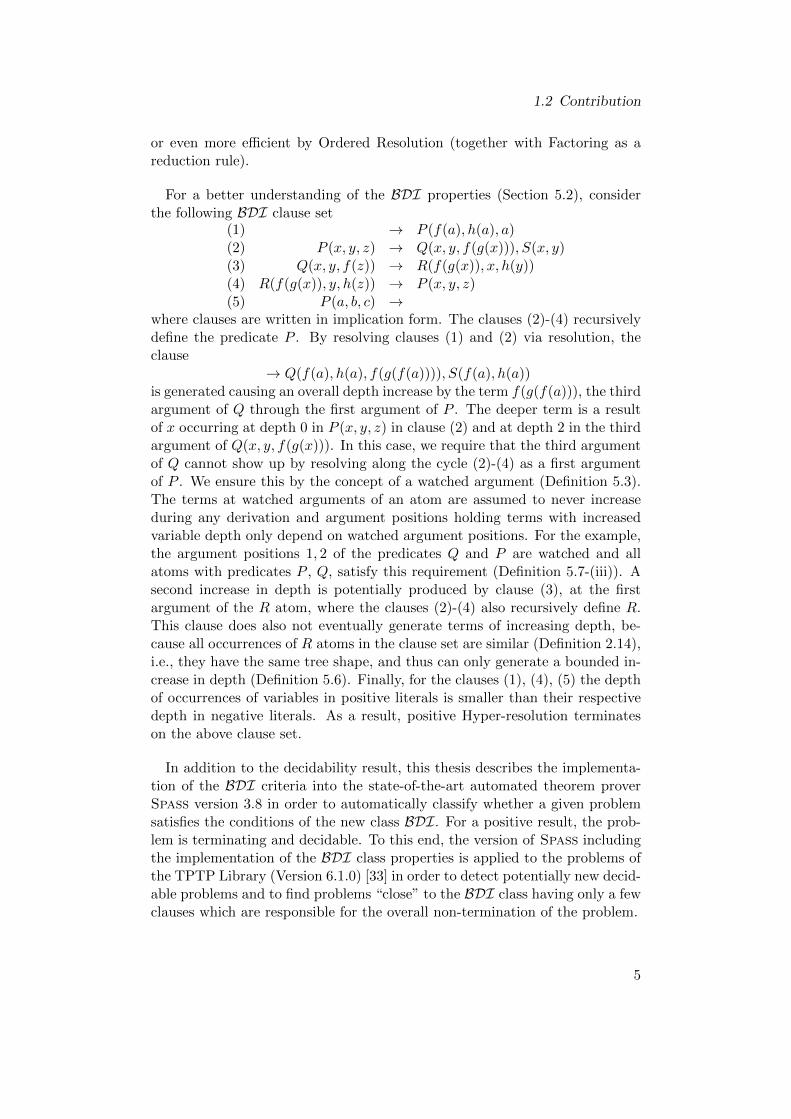
For a better understanding of the BDI properties (Section 5.2), considerthe following BDI clause set
(1) → P (f(a), h(a), a)(2) P (x, y, z) → Q(x, y, f(g(x))), S(x, y)(3) Q(x, y, f(z)) → R(f(g(x)), x, h(y))(4) R(f(g(x)), y, h(z)) → P (x, y, z)(5) P (a, b, c) →
where clauses are written in implication form. The clauses (2)-(4) recursivelydefine the predicate P . By resolving clauses (1) and (2) via resolution, theclause
→ Q(f(a), h(a), f(g(f(a)))), S(f(a), h(a))is generated causing an overall depth increase by the term f(g(f(a))), the thirdargument of Q through the first argument of P . The deeper term is a resultof x occurring at depth 0 in P (x, y, z) in clause (2) and at depth 2 in the thirdargument of Q(x, y, f(g(x))). In this case, we require that the third argumentof Q cannot show up by resolving along the cycle (2)-(4) as a first argumentof P . We ensure this by the concept of a watched argument (Definition 5.3).The terms at watched arguments of an atom are assumed to never increaseduring any derivation and argument positions holding terms with increasedvariable depth only depend on watched argument positions. For the example,the argument positions 1, 2 of the predicates Q and P are watched and allatoms with predicates P , Q, satisfy this requirement (Definition 5.7-(iii)). Asecond increase in depth is potentially produced by clause (3), at the firstargument of the R atom, where the clauses (2)-(4) also recursively define R.This clause does also not eventually generate terms of increasing depth, be-cause all occurrences of R atoms in the clause set are similar (Definition 2.14),i.e., they have the same tree shape, and thus can only generate a bounded in-crease in depth (Definition 5.6). Finally, for the clauses (1), (4), (5) the depthof occurrences of variables in positive literals is smaller than their respectivedepth in negative literals. As a result, positive Hyper-resolution terminateson the above clause set.
In addition to the decidability result, this thesis describes the implementa-tion of the BDI criteria into the state-of-the-art automated theorem proverSpass version 3.8 in order to automatically classify whether a given problemsatisfies the conditions of the new class BDI. For a positive result, the prob-lem is terminating and decidable. To this end, the version of Spass includingthe implementation of the BDI class properties is applied to the problems ofthe TPTP Library (Version 6.1.0) [33] in order to detect potentially new decid-able problems and to find problems “close” to the BDI class having only a fewclauses which are responsible for the overall non-termination of the problem.
5

1 Introduction
1.3 Related Work
The identification of decidable fragments of first-order logic has a long tra-dition in automated reasoning research. It started with the specification ofdecidable quantor prefix classes at the beginning of the 20th century: Bernays-Schonfinkel, Ramsey, Ackermann, Godel, Kalmar, Schutte (see [8] for anoverview). After the invention of automated reasoning calculi, in particu-lar resolution-based calculi, it moved to the identification of decidable clauseclasses (e.g., see [6, 35, 12, 17, 19, 1]) which then serve, e.g., as (background)fragments for effective reasoning on tree automata properties, reachabilityproblems in security, knowledge representation formalisms, or data structures.
The BDI class presented in this thesis is not included in any known decid-able clause class. It generalizes the well-known class PVD [12]. The class ofguarded formulas, originally proposed by Andreka et al. [27], was shown tobe decidable through an effectively bounded finite model property. The firstresolution decision procedure for the guarded fragment has been described byde Nivelle [28]. It has been further studied by Georgieva et al. [14] resulting inthe fragment GF1−, for which Hyper-resolution is a decision procedure. Theclass GF1− includes function symbols but does not support non-guarded for-mulas. For example, a transitivity clause is not included in this fragment butcontained in our class BDI. Further classes that can be decided by resolution(superposition) without generating clauses with a term depth increase are themonadic class [6], the class of shallow sort theories [35], or classes related totree automata [19].
Another related class is BU [15], which generalizes the set of all clause setsone can obtain from GF1−, includes function symbols, and is also decidable byHyper-resolution. The class definition of BU takes special care of variables, forexample, every non-positive functional clause must contain a covering negativeliteral which contains all the variables of the clause. Eventually this limits thedepth of clauses generated by Hyper-resolution. In BDI, we don’t requiresuch conditions but instead limit the form of recursive definitions.
A completely different way to deal with the problem of termination is themethod proposed by Baumgartner et al. [7]. It reduces model search first toa sequence of satisfiability problems made of function-free first-order clausesets, and then applies a theorem prover to the transformed (decidable) prob-lem. However, this method also comes with several drawbacks. One is that thetransformation is not unsatisfiability preserving unless left-totality is forced.Consider the following (unsatisfiable) clause set (in implication form) as anexample:
(1) → P (g(x), a)(2) P (g(b), y) →
Obviously, simple resolution between these two clauses yields the empty clause.The proposed transformation (without the left-totality) leads to the new clauseset
6
1.3 Related Work
(1′) Ra(z), Rg(x, y) → P (y, z)(2′) Rb(z), Rg(z, x), P (x, y) →
which is not unsatisfiable anymore. The left-totality for restoring unsatisfiabil-ity consists of a skolemized version of the axiom ∀x1, . . . , xn∃yRf (x1, . . . , xn, y)for all function symbols f , which causes an expansion of the signature of theproblem in size of the number of domain elements. In the context of SAPauthorizations with large domains, this would cause a massive increase of thegeneration of ground facts during saturation. This obvious problem of scala-bility towards larger domain sizes is known by the authors and has also beenmentioned as a main area of further research in their paper. A second maindisadvantage is the missing (value) symmetry breaking mechanism for functionsymbols of arity greater than one. A constraint satisfaction problem exhibitsvalue symmetry if permuting the values of a partial solution for the problemgives another partial solution. For BDI classes, this is not a problem becausethere is no transformation applied to a given set of clauses and the terminationis guaranteed mainly by limiting the form of recursive definitions.
7

2 Foundations
2.1 Mathematical Foundations
This chapter recalls basic definitions of first-order logic as well as the fun-damentals of first-order theorem proving which are used in this thesis. Thedefinitions are basically taken from [36], and [5], and the relations on termsfrom [2]. Further, it recaps the definition and properties of graphs.
Definition 2.1 (Natural Numbers)The set N of natural numbers contains all non-negative integers, i.e., N ={0, 1, 2, . . .}.
Definition 2.2 (Multisets)A multiset over a set A is a function M : A → N. Intuitively, M(a) specifiesthe number of occurrences of a in M . If M(a) > 0 then a is an element ofM , otherwise M is called empty . Like the empty set, the empty multiset isdenoted by ∅. The union of two multisets M1 and M2 with x ∈ A is definedby (M1 ∪M2)(x) = M1(x) +M2(x). Analogously, the intersection of M1 andM2 with x ∈ A is defined by (M1 ∩M2)(x) = min{M1(x),M2(x)}.
Multisets are described by using a set-like notation. For example, {x, x, x}denotes the multiset M where M(x) = 3 and M(x′) = 0 for all x′ 6= x in A.
Definition 2.3 (Orderings)A partial ordering � on a set M is a binary relation on M that is
(i) reflexive, i.e. a � a for all a ∈M ,
(ii) antisymmetric, i.e., a � b and b � a implies a = b for all a, b ∈M , and
(iii) transitive, i.e. a � b and b � c implies a � c for all a, b, c ∈M .
A strict partial ordering � on a set M is a binary relation on M that is
(i) irreflexive, i.e., a 6� a for all a ∈M , and
(ii) transitive, i.e., a � b and b � c implies a � c for all a, b, c ∈M .
If = is the identity relation on M and � is a partial ordering on M , then therelation � defined as � = (�\=) is a strict partial ordering. Conversely, if �is a strict partial ordering on M , then the relation � defined as � = (� ∪=)is a partial ordering.
A partial ordering � is total or an ordering on M ′ ⊆ M if a � b or b � afor all a, b ∈ M ′. A strict partial ordering � is total or a strict ordering onM ′ ⊆M if a � b or b � a or a = b for all a, b ∈M ′.
9
2 Foundations
Definition 2.4 (Lexicographic and Multiset Orderings)Let M,N be sets. The multiset extension �mul of a strict partial ordering �is defined as follows: M �mul N if
(i) M 6= N , and
(ii) for all n ∈ N \M there exists an m ∈M \N with m � n.
The lexicographic extension �lex on tuples of length n of some strict order �is defined as: (t1, . . . , tn) �lex (s1, . . . , sn) if for some 1 ≤ i ≤ n holds
(i) tj = sj for all 1 ≤ j < i, and
(ii) ti � si.
Definition 2.5 (Minimal and Maximal Elements)Let � be a strict partial ordering on a set M and let N be a subset of M ora multiset over M . With respect to � and N , an element a ∈ N is called
• maximal if there is no element b ∈ N with b � a,
• minimal if there is no element b ∈ N with a � b,
• strictly maximal if a is maximal and, if N is a multiset, N(a) = 1,
• strictly minimal if a is minimal and, if N is a multiset, N(a) = 1.
Definition 2.6 (Well-Foundedness)Let M be a set. A (strict) partial ordering � is called well-founded (Noethe-rian), if there is no infinite descending chain a0 � a1 � a2 � . . . withai ∈M, i ∈ N.
2.2 First-Order Logic
2.2.1 Syntax
This section introduces the syntax of the first-order language without equalityused within this thesis, especially terms, clauses, and formulas. We follow thenotation of [36] and [29].
Terms and Formulas
Definition 2.7 (Signature)A first-order language is constructed over a Signature Σ = (F ,R) with
(i) F is a non-empty, in general infinite set of function symbols, and
(ii) R is a non-empty, in general infinite set of predicate symbols.
10

2.2 First-Order Logic
Additionally, every function or predicate symbol has some fixed arity : F ∪R →N. A function symbol f with arity(f) = 0 is called a constant .
The letters P and Q are typically used as predicate symbols, f, g as functionsymbols, and u, v, x, y, z as variables.
Definition 2.8 (Terms)Let X be an infinite set of variable symbols disjoint from the symbols in thesignature Σ. The set of all terms T (F ,X ) is recursively defined by:
(i) every function symbol c ∈ F with arity zero (constant) is a term,
(ii) every variable x ∈ X is a term, and
(iii) whenever t1, . . . , tn are terms and f ∈ F is a function symbol witharity(f) = n, then f(t1, . . . , tn) is also a term.
A term not containing any variable is a ground term.
To improve readability, a list t1, . . . , tn of terms is often written as ~t ifthe counter variable n is obvious from the context or the concrete value ofthe upper bound is not important. Otherwise, in case we explicitly want tomention that the counter variable runs from 1 to n, we write ~tn. Also, there isthe n-fold application f(. . . (f(t)) . . .) of a unary function symbol f to a termt for which we write in short fn(t).
Definition 2.9 (Atoms)Let Σ = (F ,R) be a signature, t1, . . . , tn ∈ T (F ,X ), and P ∈ R is a predicatesymbol with arity(P ) = n. Then, P (~t) is an atom over the signature Σ.
Definition 2.10 (Formulas)Let Σ be a signature. The set of first-order formulas is inductively defined interms of atoms over Σ as follows:
(i) every atom is a formula,
(ii) the two logical constants > and ⊥ (true and false) are formulas,
(iii) if φ1, φ2 are formulas, so are ¬φ1 and φ1 ∧ φ2 and φ1 ∨ φ2, and
(iv) if x ∈ X and φ is a formula, then ∃x.φ and ∀x.φ are formulas.
The formulas occurring in this thesis are written in implication form, Γ→ ∆,where Γ contains the negative atoms and ∆ the positive atoms. For example,a formula ∀x.¬φ1 ∧ φ2 is stated as ∀x.φ1 → φ2.
Definition 2.11 (Literals, Clauses)An atom A or the negation of an atom ¬A is called literal . Disjunctions ofliterals are clauses where all variables are implicitly universally quantified.Clauses are often denoted by their respective multisets of literals where themultisets are written in usual set notation. Alternatively to the multiset no-tation of clauses, clauses are written in implication form Γ → ∆ where the
11

2 Foundations
multiset Γ is called antecedent and the multiset ∆ is called succedent of theclause. The atoms in Γ denote negative literals while the atoms in ∆ de-note the positive literals in a clause. A clause is called a unit clause if itcontains only one literal. The empty clause with Γ = ∆ = ∅ is denoted by�. A clause is Horn if ∆ contains at most one atom. We often abbreviatedisjoint set union with sequencing, e.g., we write Γ → ∆, R(t1, . . . , tn) forΓ→ ∆\{R(t1, . . . , tn)} ∪ {R(t1, . . . , tn)}.
Definition 2.12 (Variables of Terms and Atoms)The set of free variables of an atom P , term f is denoted by
(i) vars(P (t1, . . . , tn)) = ∪ivars(ti),
(ii) vars(f(t1, . . . , tn)) = ∪ivars(ti), and
(iii) vars(x) = {x}.The function naturally extends to literals, clauses and (multi)sets of terms(literals, clauses).
Definition 2.13 ((Inner) Positions, Length)A position is a word over the natural numbers. Let f(t1, . . . , tn) be a term.The set pos(f(t1, . . . , tn)) of positions of a term is recursively defined as:
(i) the empty word ε is a position in any term t and t|ε = t
(ii) if t|p = f(t1, . . . , tn), then p.i is a position in t for all i = 1, . . . , n andt|p.i = ti.
An alternative notation for t|p = s is t[s]p. The term (atom) obtained from tby replacing t|p in t with s is denoted by t[p/s] where p ∈ pos(t).
The length of a position p is defined by length(ε) = 0 and length(i.r) =1 + length(r). The notion of a position can be extended to atoms, literals andeven formulas in the obvious way.
Let p be an arbitrary position of a term s (atom, literal). We call p an innerposition if there exists a position q in s such that q = p.r, r 6= ε.
Definition 2.14 (Similarity)Let p be an arbitrary position of a term s (respectively, atom or literal). Twoatoms P (t1, . . . , tn) and Q(s1, . . . , sm) are called similar if pos(P (t1, . . . , tn)) =pos(Q(s1, . . . , sm)) and for all inner positions p we have P (t1, . . . , tn)|p =Q(s1, . . . , sm)|p, implying P = Q and n = m.
Definition 2.15 (Depth, Occurrences)The depth of a term is the maximal length of a position in the term, forexample, depth(t) = max({length(π) | π ∈ pos(t)}). The depth of a literal[¬]P (t1, . . . , tn) is the maximal depth of its terms: depth([¬]P (t1, . . . , tn)) =max({depth(t1), . . . , depth(tn)}). The depth of a clause is the maximal depthof its literals, and in the same manner, the depth of a set of literals is themaximal depth of its literals. Additionally, the function depth is extended to
12
2.2 First-Order Logic
variables and clauses (or sequences of literals) such that depth(x,C) returnsthe maximal depth of an occurrence of the variable x ∈ vars(C) of a clause C.
Let occ be a function returning the number of occurrences of a term s in aterm t, defined by
occ(s, t) = |{p ∈ pos(t) | t|p = s}|.
Substitutions
Definition 2.16 (Substitutions)A substitution σ is a mapping from the set of variables X to the set of termsT (F ,X ) such that xσ 6= x for only finitely many x ∈ X . The domain of asubstitution σ is defined as dom(σ) = {x | xσ 6= x} and the co-domain of σas cdom(σ) = {xσ | xσ 6= x}. A ground substitution σ has no variable occur-rences in its co-domain, i.e., vars(cdom(σ)) = ∅. An injective substitution σwhere cdom(σ) ⊂ X is called a variable renaming .A substitution σ can be lifted to terms T (F ,X ) by f(t1, . . . , tn) = f(t1σ, . . . , tnσ)for all f ∈ F with arity n. Likewise, the application of σ to literals and clausesis defined as:
(i) P (t1, . . . , tn)σ = P (t1σ, . . . , tnσ)
(ii) (¬P (t1, . . . , tn))σ = ¬P (t1σ, . . . , tnσ)
(iii) {A1, . . . , An}σ = {A1σ, . . . , Anσ}(iv) (Γ→ ∆)σ = Γσ → ∆σ.
Definition 2.17 (Unifiers and Most General Unifiers)Given two terms (atoms) s, t, a substitution σ is called a unifier for s and tif sσ = tσ. It is called a most general unifier (mgu) if for any other unifier τof s, t there exists a substitution λ with σλ = τ . A substitution σ is called amatcher from s to t if sσ = t. The notion of an mgu is extended to atoms andliterals in the obvious way. We say that σ is a unifier for a sequence of terms(atoms, literals) t1, . . . , tn if tiσ = tjσ for all 1 ≤ i, j ≤ n and σ is an mgu ifin addition for any other unifier τ of t1, . . . , tn, there exists a substitution λwith σλ = τ .
Term and Clause Orderings
Superposition-based calculi typically limit the number of possible inferencesby considering only clauses where the involved literals are maximal. This isadmissible because the eventual proof of the input clauses still remains correct(model existence problem, [3]), and is realized by using ordering conditionsthat are stated on the term level, and which are then extended to literaloccurrences in a clause, and to clauses (see Definition 2.20).
Popular orderings are the Knuth-Bendix ordering (KBO) [22, 10], the lex-icographic path ordering (LPO) [21], and the recursive path ordering with
13

2 Foundations
status (RPOS) [10]. In this thesis (and within our usage of the prover Spass),we use the KBO. For a broader introduction to orderings, consider the bookby Baader and Nipkow [2].
Definition 2.18 (Precedence, Weight)Let Σ = (F ,R) be a finite signature. The strict partial ordering > on thesymbols in Σ is called a precedence. Let weight : Σ → N be a weight func-tion. We call a weight function admissible for some precedence if for everyunary function symbol f with weight(f) = 0, the function f is maximal in theprecedence, i.e., f ≥ g for all other function symbols g.
The function weight is extended to a weight function on terms weight :T (F ,X )→ N as follows:
(i) if t ∈ X then weight(t) = k, where k = min({weight(c) | c ∈ F , arity(c) =0}), and
(ii) t = f(t1, . . . , tn), then weight(t) = weight(f) +∑
i weight(ti).
Definition 2.19 (Kuth-Bendix Ordering)Let s, t ∈ T (F ,X ) be two terms, then t �kbo s if occ(x, t) ≥ occ(x, s) for everyvariable x ∈ (vars(t) ∪ vars(s)) and
(i) weight(t) > weight(s), or
(ii) weight(t) = weight(s) and t = f(t1, . . . , tn) and s = g(s1, . . . , sm) and
(2a) f > g in the precedence, or
(2b) f = g and
(2b1) (t1, . . . , tn) �lexkbo (s1, . . . , sm) or
(2b2) (tn, tn−1, . . . , t1) �lexkbo (s1, sm−1, . . . , s1)
If the precedence > is total on Σ then the KBO is total on ground terms(atoms).
Definition 2.20 (Literal/Clause ordering)Let � be a (reduction) ordering on terms/atoms. It can be extended to clausesas follows: Clauses are considered as multisets of occurrences of atoms. Theoccurrence of an atom A in the antecedent of a clause is identified with themultiset {{A,>}}, the occurrence of A in the succedent with {{A}, {>}}. Theconstant > is always assumed to be minimal with respect to �. Additionally,the symbol � is overloaded on literal occurrences to be the twofold multisetextension of � on terms (atoms) and � on clauses to be the multiset extensionof � on literal occurrences. If � is well-founded (total) on terms (atoms), soare the multiset extensions on literals and clauses.
Definition 2.21 (Reductive Clause)A clause Γ→ ∆, A is called reductive for the atom A if the atom A is a strictlymaximal occurrence of an atom in the clause.
14
2.3 First-Order Reasoning
2.2.2 Semantics
Definition 2.22 (Herbrand Interpretation)A Herbrand interpretation I is a set of ground atoms. A ground atom A issaid to be true in I if A ∈ I. It is called false in I if A /∈ I. The constant> is true in all interpretations, whereas ⊥ is false in all interpretations. Thelogical connectives are interpreted as usual: A conjunction A ∧B is true in Iif both A and B are true in I; a disjunction A ∨ B is true if at least one ofA and B is true; a negated atom ¬A is true in I if A /∈ I. If F is a formula,the universally quantified formula ∀x.F is true in I if Fσ is true in I forall substitutions σ that assign x to some ground term, and an existentiallyquantified formula ∃x.F is true in I if Fσ is true in I for some substitutionσ that assigns x to some ground term. A ground clause is true in I if at leastone of its literals is true in I.
Definition 2.23 (Model)An interpretation I is called a model of a formula F if F is true in I and iswritten as I |= F . Similarly, for two formulas F1, and F2, F1 |= F2 denotes thatwhenever F1 is true in I then also F2 is true in I. An alternative notationis I |= F2 whenever I |= F1. If C1, . . . , Cn and D are clauses, we writeC1, . . . , Cn |= D if for all Herbrand interpretations I whenever I |= C1, . . . , Cnthen also I |= D. For a set of clauses N , we say I is a model of N , writtenI |= N if I |= C for all clauses C ∈ N .
Definition 2.24 (Satisfiability)Let N be a clause set. N is called satisfiable if there is a Herbrand interpre-tation I with I |= N . Otherwise, N is called unsatisfiable.
2.3 First-Order Reasoning
First-order theorem proving deals with the problem of showing whether agiven clause (formula) C is a logical consequence of a set of clauses N , writtenas N |= C. The proof is usually done the other way around by showingthe inconsistency of the set N ∪ {¬C}. This inconsistency is established byproviding a formal proof of ⊥ from N by means of appropriate calculi whichare described by a collection of inference and reduction rules that determinehow new clauses can be derived from the given clauses.
Let Res�S be the calculus – the inference and reduction rules – used inthis thesis which is presented in detail in the following sections. It uses theresolution calculus of Bachmair and Ganzinger [5] that is based on generalresolution due to Robinson [31]. The rules are given in a generic way suchthat each definition covers several variants of the rule. In particular, therules are parameterized by an admissible ordering � on literals and a selectionfunction S. The admissible ordering is a total (well-founded) strict ordering
15
2 Foundations
on the ground level for the literals and extended to the non-ground level ina canonical manner. The selection function assigns to each clause a possiblyempty set of occurrences of negative literals with the effect that all inferencerule applications taking this clause as a parent clause must involve the selectedliterals [36]. Note that the selection restriction of negative literals does notdestroy completeness [4].
2.3.1 Inferences
Given the calculus Res�S , one way of altering a given clause set N is to useinferences with premises in N to derive new clauses. The other way is toeliminate so-called redundant clauses which is described in Section 2.3.2.
An inference is a relation on clauses where the elements of such a relationare written as
C1 = Γ1 → ∆1 . . . Cn = Γn → ∆n
D = Γ→ ∆
The clauses C1, . . . , Cn are called the premises, and D the conclusion or re-solvent of the inference. The conclusion of the inference is eventually addedto the given clause set N . A set of inferences is called an inference system.
The closure of clause sets under the calculus Res�S in this thesis is given by
Res(N) = {C | C is a conclusion of an inference or
reduction rule with premises in N},Res0(N) = N ,
Resn+1(N) = Res(Resn(N)) ∪ Resn(N) for n ≥ 0, and
Res∗(N) =⋃n≥0
Resn(N).
A set of clauses N is called saturated (with respect to the inferences of thecalculus Res) if Res∗(N) ⊆ N . A set N of clauses that has been altered by nsteps of inferences (and reductions) is written as Resn(N). If the exact numbern is not known or not important, the altered set N is referred to as N∗.
This thesis makes use of the following inference rules. The terminationproof of the BDI clause class even computes inferences only using the belowmentioned ordered hyper-resolution rule. As usual the calculus Res is basedon a reduction ordering � that is total on ground terms.
Definition 2.25 ((Ordered) Hyper-Resolution)The inference
E1, . . . , En → ∆ → ∆i, E′i (1 ≤ i ≤ n)
(→ ∆,∆1, . . . ,∆n)σ
where
16
2.3 First-Order Reasoning
(i) σ is the simultaneous mgu of E1, . . . , En, E′1, . . . , E
′n,
(ii) all E′iσ are strictly maximal in (→ ∆i, E′i)σ
is called an ordered hyper-resolution inference. If condition (ii) is dropped, theinference is called a hyper-resolution inference.
Definition 2.26 ((Ordered) Resolution)The inference
Γ1 → ∆1, E1 E2,Γ2 → ∆2
(Γ1,Γ2 → ∆1,∆2)σ
where
(i) σ is the mgu of E1 and E2,
(ii) no literal in Γ1 is selected,
(iii) E1σ is strictly maximal in (Γ1 → ∆1, E1)σ,
(iv) the atom E2σ is selected or it is maximal in (E2,Γ2 → ∆2)σ, and noliteral in Γ2 is selected
is called an ordered resolution inference. If conditions (iii)-(iv) are replaced byE2 is selected or no literal is selected in Γ2, the inference is called resolution.
Definition 2.27 ((Ordered) Factoring)The inferences
Γ→ ∆, E1, E2
(Γ→ ∆, E1)σ
andΓ, E1, E2 → ∆
(Γ, E1 → ∆)σ
where
(i) σ is the mgu of E1 and E2,
(ii) (E1, E2 occur positively, E1 is maximal and no literal in Γ is selected), or(E1, E2 occur negatively, E1 is maximal and no literal in Γ is selected orE1 is selected),
is called ordered factoring right and ordered factoring left , respectively. Ifcondition (ii) is replaced by (E1, E2 occur positively and no literal in Γ isselected) or (E1, E2 occur negatively, E1 is selected or no literal in Γ is selected)the inferences are called factoring right and factoring left , respectively.
17

2 Foundations
2.3.2 Reductions
Along with using inferences, there is the way of using reductions on a givenclause set N . If clauses in a set N∗ are already implied by smaller clausesin N∗, they can be eliminated using the reduction rules given below. Theconcept of redundancy is used to reduce the number of clauses that need to beconsidered as premises for future inference steps. In general, a clause is calledredundant with respect to a set of clauses N , if it follows from clauses in Nthat are smaller than C.
Definition 2.28 (Subsumption)The reduction
Γ1 → ∆1
Γ2 → ∆2
where Γ2σ ⊆ Γ1 and ∆2σ ⊆ ∆1 for some substitution σ is called subsumption.
Definition 2.29 (Condensation)The reduction
Γ1 → ∆1
Γ2 → ∆2
where Γ2 → ∆2 subsumes Γ1 → ∆1 and Γ2 → ∆2 is derived from Γ1 →∆1 by instantiation and (exhaustive) application of trivial (duplicate) literalelimination is called condensation.
For the purpose of this thesis the reduction rules subsumption and condensa-tion suffice. Nevertheless, the calculus could be enhanced by all simplificationrules which are compatible with the general notion of redundancy.
Now the (ordered) hyper-resolution calculus consists of the rules (ordered)hyper-resolution, (ordered) factoring, subsumption deletion, and condensa-tion. The (ordered) resolution calculus consists of the rules (ordered) resolu-tion, (ordered) factoring, subsumption deletion, and condensation.
Reduction rules are applied exhaustively and before the application of anyinference rule.
2.3.3 Soundness and Completeness
The most important properties of every calculus are soundness and complete-ness. Soundness means that only inferences can be made that do not changethe semantics of the problem while completeness entails that if a resolvent isa logical consequence then it can also be derived by the calculus.
The calculus Res�S used in this thesis by Bachmair and Ganzinger is soundand refutationally complete [5]. The following gives the formal definition:
Definition 2.30The calculus Res�S is sound and refutationally complete with respect to a setN of clauses if N |= ⊥ ⇔ ⊥ ∈ N .
18
2.4 Graphs
2.4 Graphs
A graph is a representation of a set of objects (vertices), where some of themhave relations with other objects. The relations are represented by graphicallinks (edges). The following gives a formal definition of a graph, and is basedon [11, 34].
Definition 2.31A graph G consists of a set of vertices V and a set of edges E. If each edge inE is an ordered pair (v, w) of vertices in V , the graph is directed , or, if eachedge in E is an unordered pair {v, w} of vertices in V , the graph is undirected .
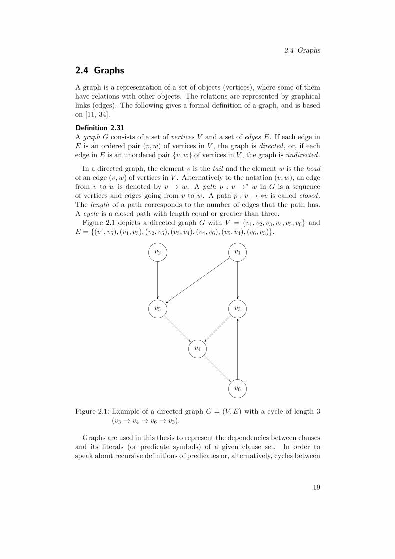
In a directed graph, the element v is the tail and the element w is the headof an edge (v, w) of vertices in V . Alternatively to the notation (v, w), an edgefrom v to w is denoted by v → w. A path p : v →∗ w in G is a sequenceof vertices and edges going from v to w. A path p : v → ∗v is called closed .The length of a path corresponds to the number of edges that the path has.A cycle is a closed path with length equal or greater than three.
Figure 2.1 depicts a directed graph G with V = {v1, v2, v3, v4, v5, v6} andE = {(v1, v5), (v1, v3), (v2, v5), (v3, v4), (v4, v6), (v5, v4), (v6, v3)}.
v6
v4
v5 v3
v2 v1
Figure 2.1: Example of a directed graph G = (V,E) with a cycle of length 3(v3 → v4 → v6 → v3).
Graphs are used in this thesis to represent the dependencies between clausesand its literals (or predicate symbols) of a given clause set. In order tospeak about recursive definitions of predicates or, alternatively, cycles between
19

2 Foundations
clauses for a given clause set, the following notion of reachability between pred-icate symbols of atoms occurring in (possibly different) clauses is establishedby means of graphs.
Definition 2.32 (Reachability)Given a clause set N and its directed graph G with V = R (all predicatesymbols) and edges E = {(P,Q) | C = Γ, P (~x) → ∆, Q(~y)}) for all clausesC ∈ N with corresponding predicate symbols P,Q.
A predicate Q is reachable from P in one step if it exists an edge (P,Q) inG. Moreover, a predicate R is reachable from P if (P,R) ∈ E or if it exists apath P →∗ R.
20

3 The SAP (Authorization) System
During the last decades a lot of mid-size and large companies introduced ERP(Enterprise Resource Planning) software like the SAP system.
The SAP systems have a long tradition. It started with a financial Account-ing system named R/1 R© which was then replaced by the SAP R/2 R© systemat the end of the 1970s. The SAP R/2 R© system was in a mainframe basedbusiness application software suite that was very successful in the 1980s andearly 1990s. In 1992, with the introduction of distributed client-server com-puting, SAP brought out a client-server based version, called SAP R/3 R©.It’s new architecture was compatible with multiple platforms and operatingsystems and allowed SAP to gain a lot of new customers. The current ver-sion SAP ERP 6.0 (formerly mySAP ERP 2005) differs from R/3 R© in theway that it builds on SAP NetWeaverTM as its platform for applications.The components based on SAP NetWeaverTM can be implemented both inABAP R© (SAP’s own programming language) or Java. The main componentof the SAP ERP 6.0 system – ERP Central Component (SAP ECC) – is thesuccessor of the R/3 R© system and consists of the following core modules:
• Financials:Financial Accounting (FI), Controlling (CO), Strategic Enterprise Man-agement (SEM), Enterprise Controlling (EC), Investment Management(IM), Public Sector Management (PSM), Project System (PS), Real Es-tate Management (RE), Treasury (TR)
• Human Capital Management (HCM), also known as Human Resources(HR):Personnel Management (PA), Personnel Time Management (PT), Pay-roll (PY), Training and Event Management (PE), Personnel Develop-ment (PD), Cost Planning (CP)
• Logistics:Materials Management (MM), Production Planning and Control (PP),Plant Maintenance (PM), Sales and Distribution (SD), Logistics Execu-tion (LE), Environment, Health & Safety (EHS), Customer Service (CS),Quality Management (QM), Logistics-General (LO), Product LifecycleManagement (PLM), Warehouse Management (WM)
• Workflow (WF)
21

3 The SAP (Authorization) System
Additionally, there are modules which are prefixed with IS (Industry Solu-tion) indicating that they combine the basic modules with additional industry-specific functionality. The following list gives an excerpt of the variety ofdifferent industry modules:
• Aerospace and Defense (IS-AD),
• Automotive (IS-A),
• Oil and Gas (IS-OIL),
• Health care (IS-H),
• Media (IS-M)
• ...
Altogether, one can see from the variety of available modules and the longhistory of SAP that it is a very successful system and the instances itself maybe very large. From the organizational point of view, a single instance of anSAP ERP system can map one department of a company (e.g., supply chainmanagement) as well as worldwide corporations with a lot of departments andsubsidiaries. Considering such large systems, it is conceivable that especiallythe administration of authorizations is highly extensive.
Concerning the different versions of SAP, I have already explored in my Mas-ters Thesis [23] that the authorization concepts of the former SAP R/3 R© sys-tem and the current releases seem to be identical. Therefore, we can simplyrefer to “The SAP System” in this thesis which means the SAP R/3 R© systemor any release after up to now.
During my work, I had access to the SAP installation of the Max-PlanckSociety which I used to acquire information about the authorization mecha-nisms and the authorizations. The Max-Planck Society uses the SAP systemrelease SAP ECC 6.0 with SAP NetWeaver 7.0 (2004s).
This chapter provides the description of the SAP system and the relevantauthorization layer that is required for the development of the formalization inChapter 4. Several paragraphs throughout the whole chapter are adopted lit-erally or in a rephrased form from my Masters Thesis [23]. Besides, Chapter 3is organized as follows.
In Section 3.1, the reader gets introduced into the different componentsrelated to authorization checks and the relationship between these elements inan authorization check procedure will be explained.
Afterwards in Section 3.2, the authorization setup structure representingthe users and their authorizations is described and how the authorizations canbe assigned to users.
Section 3.3 presents (parts of) the purchase process as a typical example ofa business process. It includes some screenshots in order to depict and to easethe understanding of the process implementation in the SAP system.
22
3.1 Authorization Checks
Eventually, Section 3.4 introduces into the concept of business policies andgives some examples related to the purchase process.
3.1 Authorization Checks
This section explains the main components used for the authorization checksstarting with a brief description of the term of a transaction in Section 3.1.1.Transactions often appear in the context of database transactions, and thisbasic understanding also applies roughly to a transaction in the SAP system.
Sections 3.1.2 and 3.1.3 describe how authorization objects and authoriza-tions are used to protect data, functions and even database tables from unau-thorized access, and also dissociate the two terms from each other.
Eventually, a complete authorization check is sketched in Section 3.1.4 whichdescribes how its execution makes use of the single components presentedbefore.
3.1.1 Transactions
Transactions are known from databases where a transaction corresponds to asingle logical operation on the data – no matter how many individual changesare required. It must fulfill the so-called ACID criteria: Atomicity, consistency,isolation, and durability.
This concept also applies to transactions in the SAP system. The program(code) where the authorization checks are attached and implemented is calledan SAP transaction. Usually, the start of a transaction implies the checkof multiple individual authorizations. According to the ACID criteria fordatabase transactions, the check of all individual authorizations for a specificuser either succeeds or fails as a group (atomicity) and cannot be interferedby authorization checks for other users running the same program (isolation).In other words, if only one individual check fails for the specific user, then theoverall transaction fails, too. The exact procedure of authorization checks isdescribed in more detail in Section 3.1.4.
The execution of the transaction in SAP corresponds to the execution of afunction in the SAP system. Then, the function starts the associated program.Every program that needs to be protected has its unique identification codewhich is called transaction code. In SAP, the term transaction is typicallyused to refer the called program itself. Short statements like “the transactionxy” denote the program where xy is the transaction code for that program.
The concrete number of individual authorization checks often differs betweenmultiple runs of a transaction. This is caused by those checks implementedusing a traditional if-else statement and which depend on the data that hasbeen entered.
23

3 The SAP (Authorization) System
Furthermore, we need to distinguish between the authorization check itselfand the checked data: If the implementation of a number of authorizationchecks for a concrete transaction doesn’t change and the number of checks isalso the same for two runs, then the checks themselves are identical (the sameaccess right is checked) in each run of the transaction, but the data is not nec-essarily equal. For example, a check in a transaction could be the verificationof the user’s department where the checked data is different because not allemployees in a company belong to the same department. In that case, thecheck for the access right itself – namely the right to access the department –for each run is equal.
3.1.2 Authorization Objects
Authorization objects are used to protect functions or data in the SAP sys-tem. Every authorization check occurring when a transaction starts or duringthe execution of a transaction checks the associated authorization object tobe present with the required values. The authorization object can be seenas a container for the authorization values. It is a logical entity that groupsbetween one and ten value fields requiring authority checking within the sys-tem. The fields can be eventually filled with different authorization values.This structure is illustrated by Figure 3.1. Already the (old) release 4.6 of
Authorization Object
Authorization Field
Authorization Field
Authorization Field Authorization
Field … 1-10
Value Field
Value Field
Value Field
Value Field
Figure 3.1: Authorization object structure.
SAP includes around 900 pre-defined authorization objects that are classifiedinto ca. 40 object classes corresponding to their application area, for exampleFinance or Human Resources. If still none of these objects is suitable, thereis the possibility to define additional authorization objects which are liable tothe structure described before.
3.1.3 Authorizations
The combination of the authorization object with concrete values having beenfilled into the value fields constitutes the authorization, that is an instance ofthe authorization object. In this way, many different instances can be created
24

3.1 Authorization Checks
Authorization Field Possible Values
ACTVT (Activity) 01 - Create02 - Change03 - View
Table 3.1: Authorization values denoting the type of an activity.
using one authorization object by filling in different values. The structure isdepicted in Figure 3.2. The term “authorization” often leads to confusion be-
Authorization Object
Authorization Field
Authorization Field
Authorization Field Authorization
Field … 1-10
Value Value Value Value
Authorization
Figure 3.2: Authorization (instance of an authorization object).
tween the everyday language terminology and the terminology used by SAPpeople. In general, an authorization is the permission of a person to do some-thing, or, translated to our scenario, the permission to execute a function ina system. However, in the SAP system and usually in this thesis (but stilldepending on the context), we refer to the authorization as the special notionfor the previously mentioned combination of the authorization object and itsfield values.
The insertable values for a value field of an authorization object can be singlevalues or also value ranges. For example, there are a number of numericalvalues available denoting the type of an activity. Table 3.1 shows some typicalactivity codes.
In addition to the previously mentioned numerical values and value ranges,one can use the wild-card characters question mark (?) and the asterisk (*).As usual, the question mark represents a single character while the asteriskstands for any combination of characters of any length. As soon as a valuecontains wild-card characters, it is called a regular pattern. However, in thisthesis, I have considered only the asterisk as the wild-card symbol and so farno composed values (in order to ease the complexity).
Authorizations are eventually used during the authorization check in theSAP system in which the built-in authorization policy forbids all actions notexplicitly permitted by an authorization. Authorizations can only grant per-
25
3 The SAP (Authorization) System
missions but not restrict or forbid them.
3.1.4 Authorization Check Procedure
Authorization checks occur whenever a user requests access to a particulartransaction. In such a case, the user’s credentials (his/her assigned autho-rizations) are checked against the requested ones and if the authorizationsmatch (both the authorization object and its values must match), the user ispermitted to access the information which is protected by the authorizationobject.
The actual authorization check consists of two parts: (i) it checks the pres-ence of the required authorization in the authorization profile of the user’smaster record (for this purpose only the authorization object name is com-pared), (ii) the comparison of the required value(s) with the value(s) presentin the value field(s) of the authorization. The check (i) is successful if therequested authorization object is available in the user’s profile. The secondcheck (ii) succeeds if all value fields with the corresponding values of the objectmatch to the required fields and values (AND-combination). Matching meansin the context of this thesis that one of the following conditions holds:
• The present value in the value field is the asterisk wild-card character(*) . This character matches any required value.
• The present value in the value field and the required value match exactly,i.e., they are equal.
As mentioned earlier, regular pattern authorization values as well as intervalsare not considered in this thesis.
Further, a successful authorization check requires both the authorizationobject existence check (i) and all single field/value checks (ii) to succeed. Ifonly one of the single checks fails, then the overall check of the authorizationfails.
There are two different cases when an authorization check is triggered duringthe execution of a transaction:
• Check at the start of a transactionThere is a special authorization object, named S TCODE, that is alwayschecked at first for every transaction before the actual program associ-ated with the transaction will be executed. This verification is set upby the system and can’t be turned off. It is possible to associate onefurther authorization object at this place and let the system check thesetwo objects before the actual program starts.
• Check during the progress of a programThis is the default case where all authorization checks are located in
26

3.2 The Authorization Setup
the program code. On the code level, an authorization check can beforced using the AUTHORITY-CHECK statement. Whenever the sys-tem reads this keyword during the execution of the program code, it willcheck the associated authorization object with its fields1. It is possibleto check one object repeatedly in a program or to group several differentauthorization objects to protect special data or a specific part of theprogram.
In earlier times, the authorization objects always had to be identified man-ually in the program code. Today this is a bit easier because SAP providesdatabase tables2 listing all these checks. Of course, if a customer doesn’t fol-low this convention and decides not to insert the checks into these tables, it isnecessary to locate the checks directly in the program code as before.
3.2 The Authorization Setup
The authorization setup is the layer on which authorizations are assigned tousers. However, authorizations assigned to users become only effective for auser and can be used in an authorization check if the authorizations are alsopresent in the authorization profile of the user’s master record.
Authorizations can be assigned to users using the following different ways:The administrator creates so-called roles or authorization profiles or uses acombination of both ways. As mentioned, the effective authorizations arealways and only stored in authorization profiles. The assignment of any au-thorization to a user on the base of a role therefore requires the creation ofthe corresponding authorization profile. All parts are shown in an overviewpicture in Figure 3.3.
The following sub-sections describe the definition of authorization profilesand roles and also explain the differences between these two terms.
3.2.1 Authorization Profiles
An authorization profile is a group of authorizations. If an authorizationprofile has been assigned to a user then he/she is authorized to access alltransactions/functions/data granted by the authorizations in the profile.
SAP distinguishes between simple (or single-level) profiles and compositeprofiles.
1It is possible to disable the check of an object but this is not important to the generalfunctionality and therefore discarded here.
2The table USOBX holds the default values for authorizations checks occuring in transactions.The customer table USOBX C is initially (during the overall system setup) filled with thecontents of the table USOBX and can be adjusted further to fit the customer’s personalneeds.
27

3 The SAP (Authorization) System
Authorization Setup
Single Role
Single Role
Single Role
Single Role Composite Role
Single Role
Single Role Single Role
Simple + Composite Profiles
Simple Profile
Simple Profile
Simple Profile
Simple Profile
Composite Profile
Simple Profile
Simple Profile
Simple Profile
Composite Profile
Simple Profile
Simple Profile
Single Role
Single Role
Single Role Composite Role
Single Role
Single Role
Single Role Composite Role
Composite Roles
Single Roles
Effective user authorizations
Profile Generator
Profile Generator Authorization Profile
Authorization Profile
Authorization Profile
Authorization Profile
Authorization Profile
Authorization Profile
Authorization Profile
Authorization Profile
Authorization Profile
Direct Transfer User master record
Step 1
Step 2
Step 3
Business Process
User executes Transaction(s): = Associated program queries the users master record within the Authorization Checks
…
Figure 3.3: Complete picture of SAP authorizations.
28
3.2 The Authorization Setup
Simple Auth. Profile
Level 1
Figure 3.4: Structure of a simple (single-level) authorization profile.
• Simple (single-level) profiles have authorizations on one level. Nestedlevels are not possible. The following Figure 3.4 shows the structure ofa simple profile. The assignment of a simple profile to a user results inthe assignment of all authorizations to the user which are contained inthe profile.
• Composite profiles can contain single profiles or other composite profiles.The notion is to reduce the maintenance effort with a better structurein the authorizations part. Therefore, a composite profile groups dif-ferent simple and/or other composite profiles together. The followingFigure 3.5 depicts the structure of a composite profile.
From the technical side there is no difference between the assignmentof a simple profile and a composite profile to a user. The assignmentof a composite profile just results in assignments of all authorizationswhich are contained at any level (union). Authorizations can only grantaccess to transactions/functions/data but they can’t forbid the access.Therefore, conflicts resulting from the union cannot occur because theunion of access grants implies again access grants and never the denial toaccess something. If, for example one profile contains only the permissionto read some data and another profile contains the permission to writethen the result is the permission to read and write the data.
The existence of the composite profiles remains from earlier releases ofSAP R/3 R© without the support for roles. SAP strongly recommends toonly use the concept of roles.[32, p. 88] The main reason concerns theability to structure. Roles offer more structure features than profiles andare the newer concept.
3.2.2 Roles
The so called Role Based Access Control (RBAC – also called role-based secu-rity) is an essential concept in SAP systems. Role-based security is a form ofuser-level security where the application doesn’t focus on the individual user’s
29

3 The SAP (Authorization) System
Composite Profile
Level 1 Level 2 Level …
Composite Profile
Simple Profile
Simple Profile
Simple Profile
Figure 3.5: Structure of a composite authorization profile.
identity; but rather on a logical role they occupy.
The concept of roles is important in SAP systems because roles offer greatpossibilities to compose structures. It is possible to create single roles as wellas composite roles and even inheritance between roles is supported. A toolcalled “SAP Profile Generator” is used to create single and composite roles.The name Profile Generator comes from the fact that an authorization profilewill be generated for each role and also after every change of the role. Thegeneration is required because authorizations are only effective for a user ifhe/she holds them in his/her master record. If a user holds authorizationsthen he/she in fact holds one or more authorization profiles which group theauthorizations.
If a role inherits properties from another role then the parent role is calledtemplate role. For example, a template role can inherit the contained autho-rizations to the child roles. Just like inheritance in programming languages,changes to the template role will be automatically applied to the derived roles.Template roles are often used to define roles having the same functionality (i.e.,allowing to execute the same transactions), but the specific different organi-zational level authorizations such as company code, purchasing organization,etc. are then defined in the child roles.
30
3.2 The Authorization Setup
Single Role
Figure 3.6: Structure of a single role.
Single Roles
The structure of a single role is similar to the authorization profile, i.e., it alsocontains authorization values. Figure 3.6 depicts the structure of a single role.
Whenever a single role is created using the Profile Generator the appropriateauthorization profile should be generated, too. A user effectively holds onlythe authorizations which are present in the (generated) authorization profileand which in turn has been assigned to the user. Therefore, the assignmentof a role to a user without the existence of the generated authorization profileis useless. This is due to the fact that authorization checks always and onlycompare the required authorizations with the authorizations present in theauthorization profile of the user’s master record. Therefore, an authorizationcheck will fail if the required authorization is only present in the role whichhas been assigned to the user and not in the user’s authorization profile.
The difference to the (direct) authorization profile is that changes to theauthorizations of a user which are grouped in auto-generated authorizationprofiles must take place through the role definition. It isn’t possible to changevalues directly in (auto-)generated profiles as it is in direct authorization pro-files.
Composite Roles
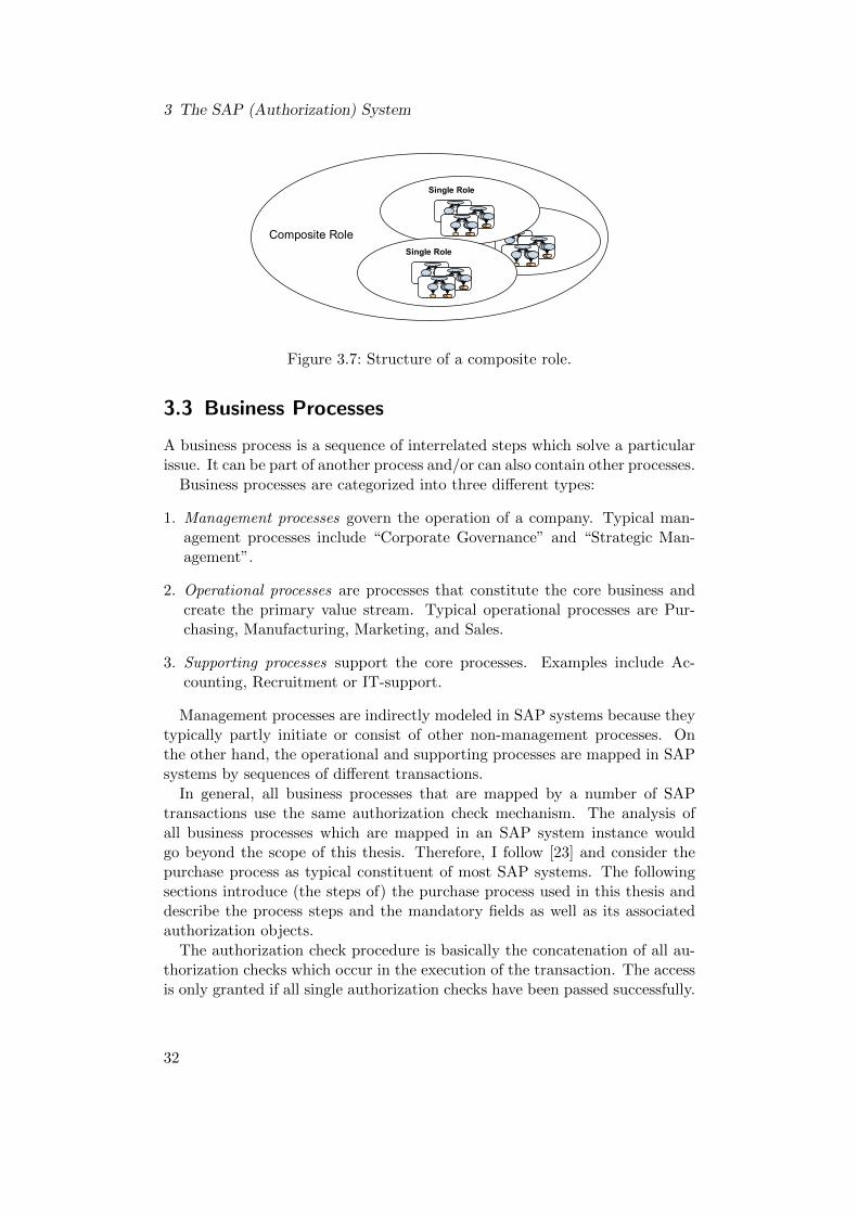
Composite roles are used for structuring and to reduce the maintenance effort.They can bundle an arbitrary number of single roles. The structure of acomposite role is shown in Figure 3.7. In contrast to a composite profile,composite roles can make use of the feature of inheritance. Therefore, thestructure capabilities are better for roles than for direct profiles.
The typical usage of a composite role is that it reflects the position of a userwith its tasks and responsibilities in a company whereas a single role holds allauthorization information needed to perform one concrete task.
31
3 The SAP (Authorization) System
Composite Role
Single Role
Single Role
Single Role
Single Role
Single Role
Single Role
Single Role
Figure 3.7: Structure of a composite role.
3.3 Business Processes
A business process is a sequence of interrelated steps which solve a particularissue. It can be part of another process and/or can also contain other processes.
Business processes are categorized into three different types:
1. Management processes govern the operation of a company. Typical man-agement processes include “Corporate Governance” and “Strategic Man-agement”.
2. Operational processes are processes that constitute the core business andcreate the primary value stream. Typical operational processes are Pur-chasing, Manufacturing, Marketing, and Sales.
3. Supporting processes support the core processes. Examples include Ac-counting, Recruitment or IT-support.
Management processes are indirectly modeled in SAP systems because theytypically partly initiate or consist of other non-management processes. Onthe other hand, the operational and supporting processes are mapped in SAPsystems by sequences of different transactions.
In general, all business processes that are mapped by a number of SAPtransactions use the same authorization check mechanism. The analysis ofall business processes which are mapped in an SAP system instance wouldgo beyond the scope of this thesis. Therefore, I follow [23] and consider thepurchase process as typical constituent of most SAP systems. The followingsections introduce (the steps of) the purchase process used in this thesis anddescribe the process steps and the mandatory fields as well as its associatedauthorization objects.
The authorization check procedure is basically the concatenation of all au-thorization checks which occur in the execution of the transaction. The accessis only granted if all single authorization checks have been passed successfully.
32

3.3 Business Processes
Determination of Material Requirements = Requisition
Determine Possible Suppliers
Select Supplier Order
Supervise the Order
Receipt of Goods
Invoice Verification
Payment
Release Requisition
Figure 3.8: The purchase process.
A more comprehensive explanation including an example about the underlyingauthorizations and authorization check procedure is available in [23].
3.3.1 The Purchase Process
The purchase process consists of several steps which are depicted in Figure 3.8.In order to keep the case study in this thesis straightforward and comprehensi-ble, we deal only with the creation of a requisition, the release and the eventualorder (marked by a box in the figure). The creation of the requisition as wellas the creation of the order is mapped by exactly one transaction in the SAPinstance of the Max Planck Society. The release transaction is mapped by twotransactions, one to view the requisition and the second to apply the release.
The following sections describe the essential data which must be enteredto successfully create the entities. This is accompanied by screenshots of thesystem to give a rough idea of the appearance of the purchase transactionscreens in the SAP system.
Create a Requisition
A purchase requisition document is created by a department and the purchas-ing group, respectively to request the purchase of goods or services. Such adocument has some mandatory fields – the fields which must be filled in orderto successfully finish the transaction. Therefore, the values of most of therequired fields are subject to authorization checks.
The list of mandatory fields contains the document type (related to the
33

3 The SAP (Authorization) System
authorization object M BANF BSA) – the type of the requisition object. Typicalvalues for this field are NB which stands for regular or “normal business”, RSUwhich stands for re-supply, or SH for special handling3.
Another mandatory field is the item number which is located in the itemarea (see Figure 3.9). It prohibits the creation of empty requisitions.
Figure 3.9: Screen to create a requisition.
Each item which is going to be purchased is destined for a concrete plant(related to the authorization object M BANF WRK). Therefore, the plant is amandatory field, too. The value depends on the structure of the company(and consequently of the customizing settings) and is typically prefilled. Anempty value suggests a non-complete customizing.
Furthermore, each item must be assigned to a concrete purchasing group(related to the authorization object M BANF EKG). The term purchasing groupis somewhat misleading because in the Max-Planck Society a purchasing groupis often composed of just one person.
Each item requires the input of either a material number or a short descrip-tion of the item. The material number is used in order to load the materialrelated data from the material master record which is stored in the database.
3The available values in a specific SAP system instance depend on the customizing settings.Customizing is the adjustment of a default SAP system to match the business needs ofa company.
34
3.3 Business Processes
Further mandatory fields like the material description, material group and theunit of measure are then prefilled automatically. The second option is to usejust the material description. Then the fields like material group and unit ofmeasure have to be filled manually.
Other required fields are, of course, the quantity of the items going to be bepurchased, the delivery date and a price valuation.
The account assignment category is also mandatory. It determines whichaccount assignment details are further required for an item (for example, thespecification of a cost center or an account number).
The screenshot depicted in Figure 3.9 shows most of the previous mentionedfields of the screen on the basis of the requisition for a Porsche sports car.
Release a Requisition
Release procedures for requisitions are used in the SAP system to approverequisitions which exceed a certain budget limit before they can be convertedto an order.
The SAP system uses so-called release strategies to achieve such approvals.They have to be defined in the customizing of the purchasing before the exe-cution of any purchase activity.
In order to provide a wide variety of possibilities the release strategies makeuse of the so-called class system which is a general component of the SAPsystem and not limited for use within release strategies. This class system isused to describe and classify any objects, for example, materials or requisitions,through characteristics in order to determine whether a certain strategy willbe applied or not.
A release typically consists of several single release steps which have to bespecified in the release strategy. Each step is defined by its release code. Therelease codes are again grouped in the release group. The so-called releaseindicators indicate the approval state of a requisition and define the possibleactions after a certain release step.
The release strategy (entity) – denoted by its release strategy name – com-bines a characteristics class, the release codes, release group, and the releaseindicators. A more detailed explanation of the release strategy and its con-stituents including some examples can be found in [23].
The screenshot depicted in Figure 3.10 shows the release screen for a requi-sition. It continues the previous example of the Porsche sports car and showsthe active release strategy VF, which stands for a management release. It con-sists of two single release steps: (i) the group leader (release code W1) and (ii) aperson of the management, for example the director (owning the release codeW2). The release of the group leader has already been passed but the directorrelease is still open and needs to be completed to fully release the requistion.
The fields that are subject to authorization checks for the release step arethe ones mentioned in Section 3.3.1, create a requisition, as well as the release
35

3 The SAP (Authorization) System
Figure 3.10: Screen to release a requisition.
36

3.4 Business Policies
group and code (together in the authorization object M EINK FRG).
Create an Order
The order is the request to the supplier or another plant of the company todeliver the requisitioned (and released) material or services under the termsand conditions agreed before.
In practice there are often negotiations with possible suppliers about theexact prices, conditions and perhaps possible discounts after the release of arequisition. If the price or the condition changes, it is typically a minimalchange. A big change results in the re-appliance of the release strategy, i.e.,either the changed item or the overall requisition has to be released again,depending on the release settings.
Assume that the release has succeeded and the conditions have not changed.A released requisition can be transformed to an order (which is connectedto the requisition) where, in contrast to the requisition, the order requiresadditionally at least accounting settings (for booking on a specific cost center,project, etc.), and a vendor.
Most of the other required fields correspond to the ones available in the req-uisition: The document type (related to the authorization object M BEST BSA),plant (related to the authorization object M BEST WRK), and purchasing group(related to the authorization object M BEST EKG). In addition, there is the fieldpurchasing organization (related to the authorization object M BEST EKO) thatis subject to authorization checks.
Figure 3.11 depicts the order step for the Porsche sports car which has beenpreviously requested and then released. After the order creation, the next stepwould be to print out the order and send it to the supplier.
The previously presented way to create orders is the default method. How-ever, companies often need additional ways to create orders because the runthrough all steps of the complete purchase process often takes a lot of time.In such cases, the process is altered to allow alternative ways to create orders.For example, an extension could allow direct orders which do not require areleased requisition but have restrictions to a certain type of material and/ora limit on the total amount of money.
3.4 Business Policies
Business policies are constraints on the business. According to the BusinessRules Group [16] a business policy or business rule is a statement that definesor constrains some aspect of the business. It is intended to assert businessstructure or to control or influence the behavior of the business. Much ofthe industry’s understanding of business policies has been historically shaped
37
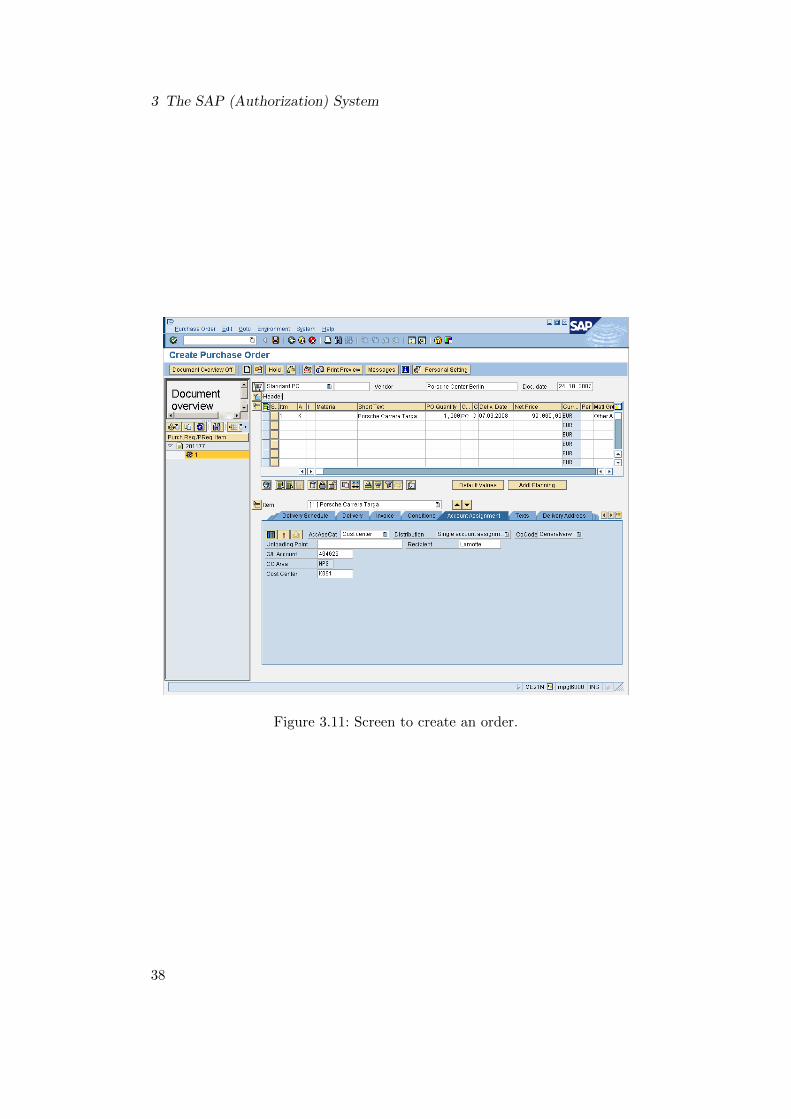
3 The SAP (Authorization) System
Figure 3.11: Screen to create an order.
38

3.4 Business Policies
by the Business Rules Group, which grouped business rules in one of fourcategories:
• Definitions of business termsThe most basic element of a business rule is the language used to ex-press it. The very definition of a term is itself a business rule whichdescribes how people think and talk about things. Thus, defining a termis establishing a category of business rule.
• Facts relating terms to each otherThe nature or operating structure of an organization can be describedin terms of the facts which relate terms to each other. To say that acustomer can place an order is a business rule. Facts can be documentedas natural language sentences or as relationships, attributes, and gener-alization structures in a graphical model.
• ConstraintsEvery enterprise constrains behavior in a non-formal way, e.g., by sayingthat a complete process cannot be executed by just one person, is closelyrelated to constraints on what data may or may not be updated. Toprevent a record from being made is, in many cases, to prevent an actionfrom taking place.
• DerivationsBusiness rules (including laws of nature) define how knowledge in oneform may be transformed into other knowledge, possibly in a differentform.
The semantic essence of a business policy expresses a logical definition ofsome facet of the organization’s way of doing business. An important featureof business policies is that they are usually specified by business people – thepeople who have responsibility for the business activities to which the rulesapply.
The business policies considered in this thesis are related to definitions,facts, and constraints. A lot of the business policy concepts are general andapplicable to many processes. However, in the context of this thesis they onlyimpose restrictions in the area of the previously presented purchase process.
Today, one best-practice approach is the Segregation of Duties or Separationof Duties (SoD). It is basically the concept of having more than one personrequired to complete a task. The use of SoD leads to individual statementsspecifying conditions and/or limitations. Each statement is a business policy.In more detail, SoD means that there is no single individual having the controlover two or more phases of a process, transaction or operation, respectively,so that a deliberate fraud is more difficult to occur because it requires col-lusion of two or more individuals or parties. There is no industry standard
39
3 The SAP (Authorization) System
for the separation of duties, but the Information Systems Audit and ControlAssociation (ISACA) has provided a segregation of duties control matrix [18],which is a general guideline suggesting which positions should be separatedand which ones require compensating controls when combined.
A further approach – which is connected to SoD – is the four-eyes princi-ple. It should be applied to critical activities or processes which should beperformed by different persons to ensure the correctness of the transactions.As in the SoD concept, the application of the four eyes principle results inconditions and limitations – the business policy statements. In this thesis, weuse a simplified form of this principle stating that the steps of a process cannotbe execute by a single user. In other words, at least two different users arerequired to execute the standard purchase process.
As mentioned above, the business policies generally impact the execution ofa business process. However, only the processes which are mapped in the SAPsystem as a sequence of transactions can be regarded. Therefore, a businesspolicy which has been specified by business people in a business terminologyhas to be implemented in the SAP system by permissions and restrictions toa set of transactions.
40
4 Formalization of the SAPAuthorization Layer
This chapter describes the main parts of the development of a formal modelrepresenting the authorization setup layer, the authorization check layer, andthe business process layer from an SAP system by first-order formulas. Itstarts by taking some abstractions into consideration in Section 4.1 whichaffect the way of construction and the structure of the resulting formulas.The construction itself is presented in detail in Section 4.2, and is based onthe work described in my Masters Thesis [23], therefore, several paragraphsthroughout the whole chapter are adopted literally or in a rephrased form frommy Masters Thesis. To the end of the formalization of the SAP authorizationlayer, the purchase process together with some typical business policies (seeSections 3.3.1 and 3.4) is reviewed under the aspects of the present formulasand the underlying structure of the resulting set of clauses.
4.1 Abstractions
The formal model presented in this thesis is based on a snapshot of an SAPsystem, i.e., the extracted authorization information (c.f. Chapter 3 for infor-mation about SAP authorizations). Correspondingly, the formal model repre-sents the system at the given time the snapshot was taken and any change ofthe authorizations requires an adjustment of the formulas.
However, the formalization presented in this thesis makes some abstractions.The first one refers to time. It would be possible to model the time when anauthorization check happens during the execution of a transaction in first-order logic but this would lead to an immense increase of the run-time oftheorem provers because of the obvious state explosion and is, at least for ourpurpose of proving termination and correctness of the authorizations and therelated business policies, not (yet) necessary.
Another assumption for the formalization are unique data. Dynamics in thedata or the authorizations are not considered. A typical example of dynamicsis a change of user authorizations while the user is performing a transaction.
The next abstraction is related to our example purchase process. We useonly one item per requisition/order which means that a new requisition/orderobject is created for each item to be purchased.
Eventually, we have not modeled pattern matching of strings with wild-card
41
4 Formalization of the SAP Authorization Layer
symbols which is used during the authorization checks and the release strategyappliance checks. We have modeled only the asterisk wild-card symbol * (butno composed values containing this symbol) matching every required value.
A more detailed description of the abstractions can be found in [23].
4.2 Construction
The formalization of the authorization setup layer considered in this thesisincludes the authorization roles and the generation of authorization profiles,and is described in Section 4.2.1. Afterwards, the formalizations of the au-thorization check and the purchase process are presented in Sections 4.2.2,and 4.2.3, respectively. The formulas are given in implication form, and if notexplicitly stated, they are universally quantified.
4.2.1 Authorization Setup
Roles
A role contains either different authorizations (single role), or in turn furtherroles with authorizations (composite role), but it isn’t possible to mix singleroles and authorizations in one composite role level.
A single role is modeled by the unary atom SingleRole. The functionauthObj() with arity 3 therein maps the authorization value to the autho-rization field of the authorization object. The authorization object togetherwith the value in turn represents the authorization which is mapped to thesingle role by the binary function singleRoleEntry().
SingleRole(singleRoleEntry(<single role name>,authObj(<auth object name>, <auth field>, <value>)))
Consider the following instance as an example:
SingleRole(singleRoleEntry( ZLAMOTTE BANF INFO,authObj( S TCODE, TCD, ME51N)))
It’s part of the single role ZLAMOTTE BANF INFO granting the permission tocreate requisitions and contains an authorization object S TCODE with the fieldTCD and the value ME51N.
A composite role is modeled using the unary atom CompositeRole. Thefunction compositeRoleEntry() therein associates the specified single role withthe composite role.
CompositeRole(compositeRoleEntry(<composite role name>,<single role name>))
42
4.2 Construction
Consider as an example the following two instances where the single rolesZLAMOTTE ORDER INFO BASE and ZLAMOTTE ORDER INFO INFO are both con-tained in the (composite) role ZLAMOTTE ORDER INFO.
CompositeRole(compositeRoleEntry( ZLAMOTTE ORDER INFO,ZLAMOTTE ORDER INFO BASE))
CompositeRole(compositeRoleEntry( ZLAMOTTE ORDER INFO,ZLAMOTTE ORDER INFO INFO))
Profile Generation and Authorization Profiles
During an authorization check the required value of an authorization is com-pared with the value in the user’s authorization profile. There are auto-generated and direct authorization profiles. Both types of profiles representauthorizations that a user holds.
The general authorization profile of a user which provides his/her effectiveauthorizations is modeled using the unary atom UserProfile. The functionuserProfileEntry() maps the different authorizations to the user:
UserProfile(userProfileEntry(<user>,authObj(<auth object name>, <auth field>, <value>)))
A concrete instance of this atom is similar to a single role instance; it alsocontains the authorization (the authorization object with its value). The dif-ference to the single role instance is that it is directly mapped to the userby the function userProfileEntry(). Of course, a complete user authorizationprofile typically consists of many single instances of this atom. The followingis an example for one instance, where the user LAMOTTE owns an authorizationobject M BANF WRK with the field WERKS and value INFO:
UserProfile(userProfileEntry( LAMOTTE,authObj( M BANF WRK, WERKS, INFO)))
The value INFO in this example enables all actions of the user LAMOTTE con-cerning purchase requisitions to the plant INFO.
The previous mentioned atom UserProfile() models the effective authoriza-tions of a user; any authorization check looks for the required authorizationin these authorization profile instances. However, authorizations cannot beassigned directly because they are contained in structures like roles (or alsodirect profiles1). Therefore, the assignment of authorizations is accomplishedby the assignment of the single or composite role to a user. This is mod-eled by the following predicate Holds denoting the fact that a user holds theauthorizations of a single or composite role.
Holds(<user>, <single role name/composite role name>)
1Using roles rather than direct profiles is best practice, hence, we concentrate on the roleshere. See [23] for more details on direct profiles.
43

4 Formalization of the SAP Authorization Layer
The effective authorization instances (represented by instances of the atomUserProfile()) are then generated automatically by a transition which firstchecks the type of the item assigned to the user via the predicate Holds,extracts the authorization part and eventually creates the user profile instance(representing the effective authorization) for the user.
4.2.2 Authorization Checks
The authorization check result – access or decline – is represented in our first-order model by the binary atom Access(). If the atom is valid, the access tothe checked authorization object is granted, otherwise it is not.
Access(<user>, authObj(<auth object name>, <auth field>, <value>))
The function authObj() with arity 3 maps the authorization value to the au-thorization field of the authorization object. The resulting authorization isthen associated with the user.
To ease specification of authorizations on a transaction base, the predicateAccess has been overloaded to model the access to an overall transaction, too.Valid instances of the following form have the meaning that all individualauthorization checks of the entire transaction have been successful.
Access(<user>, <transaction code>)
The authorization check itself compares the value of the authorization presentin the (generated) user authorization profile with the required authorization.The result of the check is indicated by validity of the predicate Access whichhas been introduced before. The formalization presented in this thesis pro-vides two basic ways to pass such an authorization check. The first way isthat the user has the exact required authorization in its authorization profile.The authorization object name, the field and the value must match. This isachieved by the following formula:
∀ xu, xaon, xaof, xav .UserProfile(userProfileEntry(xu, authObj(xaon, xaof, xav)))
→ Access(xu, authObj(xaon, xaof, xav))
The second way is that the authorization value of an authorization in theuser’s authorization profile is the wild-card symbol *. In this case, if the au-thorization objects match then the access is always granted, no matter whatthe required value is. The authorization in the user authorization profile mustcontain the constant STAR as a value which is depicted by the following tran-
44

4.2 Construction
sition.2
∀ xu, xaon, xaof, xav .UserProfile(userProfileEntry(xu, authObj(xaon, xaof, STAR)))
→ Access(xu, authObj(xaon, xaof, xav))
4.2.3 Purchase Process
The following sections describe the formalization of the purchase process as abusiness process example with its authorization checks.
Create a Requisition
The following transition shows the overloaded predicate symbol Access (intro-duced in Section 4.2.2) which models the single authorization checks that areneeded for the execution of the transaction ME51N (create a requisition). Thefirst check represents the check of the transaction code to create a requisition.The authorizations M BANF WRK, M BANF BSA and M BANF EKG have a constantin the first field (the authorization object field name like ACTVT or WERKS) anda variable value in their second field (that contains the authorization value).The atom Access(xu, ME51N) only becomes valid if the user xu has the exactconstants in his authorization profile and some value for every variable value.This means that the user is allowed to execute the transaction in at leastone instance, for example for one plant, one document type and one purchasegroup. The concrete value of the variables will and has to be evaluated andchecked at run-time when a requisition is going to be created and the exactvalues are known.
∀ xu, xwrk, xbsa, xekg .Access(xu, authObj( S TCODE, TCD, ME51N)) ∧Access(xu, authObj( M BANF WRK, ACTVT, 01)) ∧Access(xu, authObj( M BANF WRK, WERKS, xwrk)) ∧Access(xu, authObj( M BANF BSA, ACTVT, 01)) ∧Access(xu, authObj( M BANF BSA, BSART, xbsa)) ∧Access(xu, authObj( M BANF EKG, ACTVT, 01)) ∧Access(xu, authObj( M BANF EKG, EKGRP, xekg))
→ Access(xu, ME51N)
Using the grouped authorizations (denoted by the transaction code), wemodel the business process steps which typically consist of several transactions.The purchase request for an arbitrary asset is modeled by the atom Requisition
2An additional monadic atom ¬Authorization(xav) still has to be added to the formula inorder to satisfy the conditions of the new class BDI, defined in Section 5.2.
45

4 Formalization of the SAP Authorization Layer
with arity 8. The structure is described as follows:
Requisition(<document type>, <position>, <material>, <plant>,<purchasing group>, <purchasing organization>,<material group>, <price>)
Similar to the request there is the state RequisitionCreated which indicatesthat the requisition object has been created by a user in the SAP system. Thedifference to the Request is that the user who has created the requisition isnow also connected to it. This leads to an instance of the following atom witharity 9:
RequisitionCreated(<user>, <document type>, <position>, <material>,<plant>,<purchasing group>, <purchasing organization>,<material group>, <price>)
Using the previous two structures, we are now able to formally express thebusiness step which represents the creation of a requisition:
∀ xu, xbsa, xpos, xmat, xwrk, xekg, xekorg, xmatkl, xgswrt .Requisition(xbsa, xpos, xmat, xwrk, xekg, xekorg, xmatkl, xp) ∧Access(xu, ME51N) ∧Access(xu, authObj( M BANF WRK, WERKS, xwrk)) ∧Access(xu, authObj( M BANF BSA, BSART, xbsa)) ∧Access(xu, authObj( M BANF EKG, EKGRP, xekg)) ∧Access(xu, ME53N) ∧Access(xu, ME52N)
→ RequisitionCreated(xu, bsa, xpos, xmat, xwrk, xekg, xekorg,xmatkl, xgswrt)
The process starts with the existence of a purchase request modeled by theatom Requisition. In order to create a purchase requisition object in the SAPsystem, a user needs access to the corresponding transaction ME51N. The (over-loaded) atom Access(xu, ME51N) stands for the group of single authorizationchecks in this transaction. As mentioned, the variables xwrk (plant), xbsa(document type), and xekg (purchasing group) must be checked again in thesubsequent lines because only at this point the value of the variables is known(namely the value from the requisition that is going to be created). Typically,a user authorized to create a requisition is also authorized to view it or tochange it in case of a mistake. This is modeled by the lines below checkingthe access to the transactions ME53N (View) and ME52N (Change). If all con-ditions are satisfied, then the state RequisitionCreated is implied. The resultrepresents the state in the SAP system where the requisition object has beencreated.
46
4.2 Construction
Release a Requisition
The release of requisitions requires different settings in the Customizing ofpurchases. At first, these settings have to be formalized in order to apply arelease strategy to a requisition.
The first step is the definition of the release strategy. It is modeled by theatom ReleaseStrategy with arity 3.
ReleaseStrategy(<release strategy name>, <release group>,class(<characteristics class name>,
property(<property name>, <value>)))
The nested structure is required in order to obtain a formalization which isclose to the structure of the real SAP system wherein the release strategycombines a characteristics class (containing single characteristics, each givenby a property and its value(s)), the release group and code and the releasestrategy name. The binary function property() maps the value to its propertywhich is in turn mapped to the class name by the binary function class(). Atthe end, the complete characteristic is assigned to the release strategy.
Consider the release strategy VF as an example. This strategy stands fora strategy called “director release strategy”. The strategy VF in our exampleapplies when the following conditions are satisfied:
i) the plant entered in the requisition is equal to the value INFO,
ii) the specified purchasing group is equal to I26 and
iii) the total money amount of the item which is subject to the release strat-egy application check is greater than 10.000 EUR.
In the following formalization of this strategy, the different properties matchingthe fields of a requisition (FRG CEBAN WERKS=plant, FRG CEBAN EKGRP=pur-chasing group, and FRG CEBAN GSWRT=total amount of money) are groupedby the characteristics class (FRG EBAN). Further details on the release strategysetup can be found in [23].
ReleaseStrategy( VF, 01, class( FRG EBAN,property( FRG CEBAN WERKS, INFO)))
ReleaseStrategy( VF, 01, class( FRG EBAN,property( FRG CEBAN EKGRP, I26)))
ReleaseStrategy( VF, 01, class( FRG EBAN,property( FRG CEBAN GSWRT, GREATER 10000 EUR)))
Of course, we need to execute one or more single release steps dependingon the applied strategy. Each of the steps again requires a release based on
47

4 Formalization of the SAP Authorization Layer
a release group and the release code. This requirement is modeled with theatom ReleaseRequirement with arity 3.
ReleaseRequirement(<release strategy name>, <release group>,<release code>)
The following two formulas again refer to the release strategy VF – thedirector release. This release strategy consists of two steps, the cost centerrelease in the beginning (denoted by the constant W1) and the director releaseat the end (denoted by the constant W2). The constants W1 and W2 representthe respective release code in the SAP system. The release strategy and therelease codes are grouped in the release group denoted by the constant/number01. In order to perform the first release step, the releasing person needs theright release group and release code in his authorization profile.
ReleaseRequirement( VF, 01, W1)
ReleaseRequirement( VF, 01, W2)
Using the previously defined atoms it is now possible to model a releasestep. The atom RequisitionReleasedStep with arity 11 in the following formuladenotes a requisition item that has been released with a certain release groupand code. In the following transition, the requisition released step of therelease strategy xfrgstrat is valid if the requisition has been created by a userxu1, the release strategy xfrgstrat applies, the release requirement has beendefined and the authorization checks succeed for a user xu2.
∀ xu1, xu2, xbsa, xpos, xmat, xwrk, xekg, xekorg, xmatkl, xgswrt,xfrgstrat, xfrggr, xfrgco, xcl .
RequisitionCreated(xu1, xbsa, xpos, xmat, xwrk, xekg, xekorg,xmatkl, xgswrt) ∧
ReleaseStrategy(xfrgstrat, xfrggr, class(xcl,property( FRG CEBAN EKGRP,xekg))) ∧
ReleaseStrategy(xfrgstrat, xfrggr, class(xcl,property( FRG CEBAN WERKS,xwrk))) ∧
ReleaseStrategy(xfrgstrat, xfrggr, class(xcl,property( FRG CEBAN GSWRT,xgswrt))) ∧
ReleaseRequirement(xfrgstrat, xfrggr, xfrgco) ∧
Access(xu2, authObj( M EINK FRG, FRGGR, xfrggr)) ∧Access(xu2, authObj( M EINK FRG, FRGCO, xfrgco)) ∧
Access(xu2, ME54N) ∧Access(xu2, authObj( M BANF WRK, WERKS, xwrk)) ∧Access(xu2, authObj( M BANF BSA, BSART, xbsa)) ∧Access(xu2, authObj( M BANF EKG, EKGRP, xekg))
→ RequisitionReleasedStep(xu2, xfrggr, xfrgstrat, xfrgco, xbsa, xpos, xmat,xwrk, xekg, xekorg, xmatkl, xgswrt)
48
4.2 Construction
As mentioned, a release of a requisition typically consists of one ore morerelease steps. In the SAP test system of the Max-Planck Society there are tworelease strategies KF and VF. The former strategy represents the cost centerrelease and consists of one step (with the code W1). The latter strategy denotesthe already mentioned director release which consists of two steps (codes W1
and W2). Both strategies belong to the release group 01. The steps requiredfor each execution variant of the release strategy are modeled by the followingtransition. The resulting state RequisitionReleased is valid, if all requiredrelease steps have been passed.
∀ xu1, xu2, xbsa, xpos, xmat, xwrk, xekg, xekorg, xmatkl, xgswrt,xfrgstrat, xfrggr, xfrgco, xcl .
RequisitionReleasedStep(xu2, 01, KF, W1, xbsa, xpos, xmat,xwrk, xekg, xekorg, xmatkl, xgswrt) ∨
(RequisitionReleasedStep(xu1, 01, VF, W1, xbsa, xpos, xmat,xwrk, xekg, xekorg, xmatkl, xgswrt) ∧
RequisitionReleasedStep(xu2, 01, VF, W2, xbsa, xpos, xmat,xwrk, xekg, xekorg, xmatkl, xgswrt))
→ RequisitionReleased(xu2, xbsa, xpos, xmat, xwrk, xekg,xekorg, xmatkl, xgswrt)
If none of the available release strategies applies to a requisition, then it isimmediately released and ready to order. A release strategy doesn’t apply ifat least one of the properties defined in the strategy doesn’t match. So far, thetheory only contains assertions that say that a certain property matches. Inthis case, however, it is required to verify whether a property does not match.For that reason, the theory must be extended with formulas for each possiblevalue that defines when a release strategy does not apply. The followingtransition shows the transition for the plant property and its value INFO.It means, that if the value INFO matches the plant property, then, of course,other (possible) values like SOFS and MPG do not match. Similar formulas arerequired for each element of the Cartesian product of property and possiblevalue.
∀ xfrgstrat, xfrggr .ReleaseStrategy(xfrgstrat, xfrggr, class( FRG EBAN,
property( FRG CEBAN WERKS, INFO)))→ ¬ReleaseStrategy(xfrgstrat, xfrggr, class( FRG EBAN,
property( FRG CEBAN WERKS, SOFS))) ∧¬ReleaseStrategy(xfrgstrat, xfrggr, class( FRG EBAN,
property( FRG CEBAN WERKS, MPG)))
The ability to decide when a property does not match leads to the followingtransition. It models, that no release strategy (in our example neither KF norVF) applies. Therefore, the requisition is automatically released and ready foran order.
49

4 Formalization of the SAP Authorization Layer
∀ xu, xbsa, xpos, xmat, xwrk, xekg, xekorg, xmatkl, xgswrt,xfrgstrat, xfrggr, xfrgco, xcl .
RequisitionCreated(xu, xbsa, xpos, xmat, xwrk, xekg, xekorg,xmatkl, xgswrt) ∧
(¬ReleaseStrategy( KF, xfrggr, class( FRG EBAN,property( FRG CEBAN EKGRP, xekg))) ∨
¬ReleaseStrategy( KF, xfrggr, class( FRG EBAN,property( FRG CEBAN WERKS, xwrk))) ∨
¬ReleaseStrategy( KF, xfrggr, class( FRG EBAN,property( FRG CEBAN GSWRT, xgswrt)))) ∧
(¬ReleaseStrategy( VF, xfrggr, class( FRG EBAN,property( FRG CEBAN EKGRP, xekg))) ∨
¬ReleaseStrategy( VF, xfrggr, class( FRG EBAN,property( FRG CEBAN WERKS, xwrk))) ∨
¬ReleaseStrategy( VF, xfrggr, class( FRG EBAN,property( FRG CEBAN GSWRT, xgswrt))))
→ RequisitionReleased(xu, xbsa, xpos, xmat, xwrk, xekg, xekorg,xmatkl, xgswrt)
Create an Order
A successful released requisition is the precondition to create an order objectwhich is connected to the requisition in the SAP system. The following transi-tion models this business step. At first, the existence of the released requisitionis checked. It has been released by the user xu1. Then the access to the trans-action ME21N is checked because it is required to create order objects (ME22N,ME23N to edit and view orders, respectively). The last checks ensure that theuser is authorized to create orders for the plant, purchase document type, pur-chasing group and purchasing organization, respectively, which is specified bythe released requisition. All checks must succeed to enter the state OrderCre-ated. Note, that the user who has released the requisition and the user whocreates the order object can be the same person in this transition.
50
4.2 Construction
∀ xu1, xu2, xbsa, xpos, xmat, xwrk, xekg, xekorg, xmatkl, xgswrt .RequisitionReleased(xu1, xbsa, xpos, xmat, xwrk, xekg, xekorg,
xmatkl, xgswrt) ∧Access(xu2, ME21N) ∧Access(xu2, ME22N) ∧Access(xu2, ME23N) ∧Access(xu2, authObj( M BEST WRK, WERKS, xwrk)) ∧Access(xu2, authObj( M BANF BSA, BSART, xbsa)) ∧Access(xu2, authObj( M BEST BSA, BSART, xbsa)) ∧Access(xu2, authObj( M BEST EKG, EKGRP, xekg)) ∧Access(xu2, authObj( M BEST EKO, EKORG, xekorg))
→ OrderCreated(xu2, xbsa, xpos, xmat, xwrk, xekg, xekorg, xmatkl, xgswrt)
4.2.4 Business Policies
The business policies are expressed by business people in a business terminol-ogy. They impact the way of performing the business processes. For example,they prohibit the possibility for a user to perform all process steps alone. Theconnection between the business process (steps) and the SAP system is quitesimple – there is a mapping which maps a number of transactions to eachprocess step.
Our formalization already contains the mapping to the individual transac-tions, so it is easy to also model business policies.
The general but for this thesis simplified business policy that has been intro-duced in Section 3.4 prohibits the execution of the complete process consistingof the steps “create a requisition”, “release a requisition” and “create the or-der” for this requisition by one single user for one concrete plant, materialgroup, purchasing group and organization. The following formula representsthis policy: There is no requisition such that one user xu can reach all statesRequisitionCreated, RequisitionReleased and OrderCreated . Of course, the as-sumption for such a policy are unique data in the SAP system.
¬∃ xu, xbsa, xwrk, xekg, xekorg, xmatkl, xgswrt .∀ xpos, xmat .
Requisition(xbsa, xpos, xmat, xwrk, xekg, xekorg, xmatkl, xgswrt)→ RequisitionCreated(xu, xbsa, xpos, xmat, xwrk, xekg, xekorg,
xmatkl, xgswrt) ∧RequisitionReleased(xu, xbsa, xpos, xmat, xwrk, xekg, xekorg,
xmatkl, xgswrt) ∧OrderCreated(xu, xbsa, xpos, xmat, xwrk, xekg, xekorg,
xmatkl, xgswrt)
Another policy is the requirement that a corresponding requisition has tobe created before any order. This is stated by the following formula which
51

4 Formalization of the SAP Authorization Layer
expresses the fact that if we have an order created, there must exist a corre-sponding requisition.
∀ xu1, xbsa, xpos, xmat, xwrk, xekg, xekorg, xmatkl, xgswrt .∃ xu2 .
OrderCreated(xu, xbsa, xpos, xmat, xwrk, xekg,xekorg,xmatkl, xgswrt)
→ RequisitionCreated(xu2, xbsa, xpos, xmat, xwrk, xekg, xekorg,xmatkl, xgswrt)
4.2.5 Purchase Process + Business Policies Reviewed
In order to automatically prove properties by means of an automated theoremprover for clause sets resulting from authorization layer formalizations of SAPsystems, it is a good idea to show decidability for the given inputs first. This isdone by proving the input clause sets to be terminating which is only feasibleif their structure is determined and necessary (structural) properties can beestablished. Having this idea in mind, I have created a clause dependencygraph for analysis of the clauses’ structure.
Let N be the set of clauses representing a formalized SAP authorizationlayer instance. The graph is a directed graph with V = R (all predicatesymbols) and edges E = {(P,Q) |C = Γ, P (~x) → ∆, Q(~y}) for all clausesC ∈ N with corresponding predicate symbols P,Q. This graph is depicted infigure 4.1 for such a clause set.
The vertices of the graph having only outgoing edges represent the (usuallyground) facts of the authorization setup (i.e., the set of roles, authorizations,and the assignment to users), and the requirement(s) to enter the process(es)(in our example the vertices Requisition, StandardPurchase, and DirectPur-chase3 for the purchase process).
Further inspection of the graph shows that it contains a cycle with thevertices RequisitionCreated → ReleaseStrategy → RequisitionReleasedStep →RequisitionReleased → OrderCreated. The vertex RequisitionCreated is theentry point to the cycle, and OrderCreated the last vertex before we go backto the entry point. Cycles become a problem when we can execute a cyclemore than once and always derive new (and larger) clauses that have neverbeen derived before in previous loops. If this happens here, theorem proverswon’t terminate being applied to SAP authorization instances occupying thisstructure.
Therefore, I have explored the clause(s) causing the edge OrderCreated →
3This is a special variant of the purchase process where no release step is necessary but isunderlying restrictions regarding the amount of money and the type of material. See [23]for details.
52

4.2 Construction
Co
mp
osi
teR
ole
Use
rPro
file
Acc
ess
Sta
nd
ard
Pu
rch
ase
Req
uis
itio
nC
reat
ed
Req
uis
itio
nR
elea
sed
Ste
p
Req
uis
itio
nR
elea
sed
Rel
ease
Str
ateg
y
Ord
erC
reat
ed
Dir
ectP
urc
has
e
Sin
gle
Ro
le
Req
uis
itio
n
Rel
ease
Req
uir
emen
t
Pro
file
Ho
lds
Figure 4.1: Dependency graph.
53

4 Formalization of the SAP Authorization Layer
RequisitionCreated and thus closing the cycle. The culprit is
OrderCreated(xu, xbsa, xpos, xmat, xwrk, xekg, xekorg,xmatkl, xgswrt) →RequisitionCreated(f(xgswrt, xmatkl, xekorg, xekg, xwrk, xmat, xpos, xbsa),
xbsa, xpos, xmat, xwrk, xekg, xekorg,xmatkl, xgswrt)
expressing the business policy that an order cannot be created without a pre-vious requisition (c.f. Section 4.2.4). The requisition has to be created by anarbitrary user, and the item to order depends on that user. This is reflectedby the function f(xgswrt, xmatkl, xekorg, xekg, xwrk, xmat, xpos, xbsa) inthe atom RequisitionCreated(~x). Unfortunately, the overall term depth of thesuccedent in the clause above is larger than the depth of the antecedent (wehave one more function symbol, please see the definition of a depth increasingclause in Section 5.2). During the saturation process, we will derive a clausethat is larger than the parent clause (because of the function symbol f) andenter the loop again.
Further inspection shows that we have other clauses in the cycle where theterm depth of the succedent also increases compared to the antecedent part.One such candidate is the clause
RequisitionCreated(xu, xbsa, xpos, xmat, xwrk, xekg, xekorg, xmatkl, xgswrt),ReleaseGroup(xfrggr),ReleaseClass(xcl)→ ReleaseStrategy( KF, xfrggr, class(xcl,property( FRG CEBAN WERKS,xwrk))),ReleaseStrategy( VF, xfrggr, class(xcl,property( FRG CEBAN WERKS,xwrk))),RequisitionReleased(xu, xbsa, xpos, xmat, xwrk, xekg, xekorg,xmatkl, xgswrt)
representing the fact that the release strategy KF or VF is applied to a createdrequisition, or the requisition is immediately released if no release strategy isapplicable. Variants of this clause with same structure exist for all possiblecombinations of release class properties. The clause shown here employs theFRG CEBAN WERKS property matching the entered plant in the requisition. Onecan easily see that the maximum term depth in both ReleaseStrategy atomsis larger than the maximum term depth in the antecedent part. The reasonhere is the structure of the release strategy which owns a release class andproperties that are mapped to the strategy via functions.
The following Chapter lifts the mentioned structure and its inherent prob-lems to a more general theoretical level and describes, how termination canbe achieved even though there are cycles and depth increasing clauses.
54

5 The Clause Class BDI
Showing decidability for restricted subclasses of first-order logic is one of thecurrent research topics. The application of automated theorem proving infirst-order logic for verifying and proving properties in the SAP authorizationsystem considered in this thesis is a real-world application. For a practical use,general decidability of input problems given to a theorem prover, identified bya defined structure is of bigger importance than decidability only for specific(SAP) instances. Therefore, this thesis presents a class with such a definedstructure for the clauses representing the SAP authorization layer and proves itto be terminating. The typical and used way in this thesis to prove terminationis to show that both the clause size (i.e., the number of literals in a clause)and the term depth are bounded during the saturation of the input clauses.
The following clause set is a good and general example for non-terminatingresolution:
(1) → P (a, f(a))(2) P (x, y) → Q(f(g(y)), y)(3) Q(x, y) → R(f(x), x)(4) R(f(x), x) → P (f(x), x)
A quick inspection reveals the recursive definition of the predicate P throughthe clauses (2)-(4). The interested reader may notice two places of depth in-crease: (a) the variable y in clause (2) in the first argument of Q(f(g(y)), y),and (b) the variable x in clause (3) in the first argument of R(f(x), x). Aclause is generally depth increasing, if there is a variable occurring in an atomon the succedent of a clause and this occurrence is at a deeper position thanthe deepest occurrence of the same variable in the antecendent of the (same)clause. As a consequence of the depth increase, the application of (Hyper-)res-olution between the clauses (1) and (2) yields a depth increased clause
(1′) → Q(f(g(f(a))), f(a)).
Further resolution on (1′) and clause (3) produces the clause(2′) → R(f(f(g(f(a)))), f(g(f(a)))).
The resolvent (2′) in turn resolved with clause (4) then yields(3′) → P (f(f(g(f(a)))), f(g(f(a)))),
which restarts the cycle with an increased second argument f(g(f(a))) ofthe atom P (. . .) in clause (3′), compared to the atom P (a, f(a)) and its secondargument f(a) in clause (1).
In order to change this example to be terminating (without regard of thesemantics here because we’re just interested in termination), there are sev-eral possibilities: One solution is to generally prevent depth increases for all
55
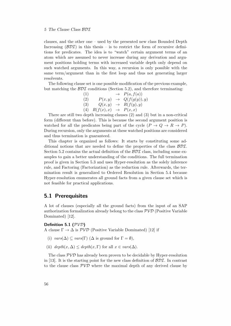
5 The Clause Class BDI
clauses, and the other one – used by the presented new class Bounded DepthIncreasing (BDI) in this thesis – is to restrict the form of recursive defini-tions for predicates. The idea is to “watch” certain argument terms of anatom which are assumed to never increase during any derivation and argu-ment positions holding terms with increased variable depth only depend onsuch watched arguments. In this way, a recursion is only possible with thesame term/argument than in the first loop and thus not generating largerresolvents.
The following clause set is one possible modification of the previous example,but matching the BDI conditions (Section 5.2), and therefore terminating:
(1) → P (a, f(a))(2) P (x, y) → Q(f(g(y)), y)(3) Q(x, y) → R(f(y), y)(4) R(f(x), x) → P (x, x)
There are still two depth increasing clauses (2) and (3) but in a non-criticalform (different than before). This is because the second argument position iswatched for all the predicates being part of the cycle (P → Q → R → P ).During recursion, only the arguments at these watched positions are consideredand thus termination is guaranteed.
This chapter is organized as follows: It starts by constituting some ad-ditional notions that are needed to define the properties of the class BDI.Section 5.2 contains the actual definition of the BDI class, including some ex-amples to gain a better understanding of the conditions. The full terminationproof is given in Section 5.3 and uses Hyper-resolution as the solely inferencerule, and Factoring (Factorization) as the reduction rule. Afterwards, the ter-mination result is generalized to Ordered Resolution in Section 5.4 becauseHyper-resolution enumerates all ground facts from a given clause set which isnot feasible for practical applications.
5.1 Prerequisites
A lot of clauses (especially all the ground facts) from the input of an SAPauthorization formalization already belong to the class PVD (Positive VariableDominated) [12].
Definition 5.1 (PVD)A clause Γ→ ∆ is PVD (Positive Variable Dominated) [12] if
(i) vars(∆) ⊆ vars(Γ) (∆ is ground for Γ = ∅),
(ii) depth(x,∆) ≤ depth(x,Γ) for all x ∈ vars(∆).
The class PVD has already been proven to be decidable by Hyper-resolutionin [13]. It is the starting point for the new class definition of BDI. In contrastto the clause class PVD where the maximal depth of any derived clause by
56
5.1 Prerequisites
Hyper-resolution does not exceed the maximal depth of its parent clauses, theclass BDI permits to have such a growth of the term depth for a derived clause.Clearly, this relaxation requires additional restrictions in order to guaranteethat Hyper-resolution still remains a decision procedure for BDI.
Definition 5.2 (Depth Increasing)We call a clause C = Γ→ P (t1, . . . , tn),∆ depth increasing if there is a variablex ∈ vars(C) and depth(x, ti) > depth(x,Γ) for some ti where 1 ≤ i ≤ n. Thevariable x is called a depth increasing variable in C, P (t1, . . . , tn) a depthincreasing atom in C, P a depth increasing predicate in C, and i a depthincreasing argument position of P .
A clause C = Γ→ P (t1, . . . , tn),∆ is called uniquely depth increasing if C isdepth increasing, and there is exactly one depth increasing argument position iof P (t1, . . . , tn) such that for all depth increasing variables x ∈ vars(C) and x /∈vars(ti) it holds depth(x, {P (t1, . . . , ti−1, ti, ti+1, . . . , tn),∆}) ≤ depth(x,Γ).Given a clause set N , a depth increasing clause C ∈ N is called a uniquelydepth increasing clause in N for the predicate P at argument position i ifthere is no different depth increasing clause for the same predicate P in Nwith depth increasing argument position j 6= i.
The later definitions of BDI speak in addition to the so far established termof reachability of predicates (Definition 2.32) about a general reachability froma depth increasing clause: A predicate symbol P occurring in a clause of aclause set N is called reachable from a depth increasing clause if there is aclause (Γ → Q(~t),∆) ∈ N , with depth increasing predicate Q, and P isreachable from Q.
Consider the following set N as a motivating example for the below defini-tion 5.3 of watched arguments:
(1) → P (f(a), b, c)(2) P (x, y, z) → Q(f(x), y, z)(3) Q(x, y, z) → P (x, y, z)
(Hyper-)resolution applied on N computes infinitely many clauses of theform Q(f i(a), b, c). The reason is, in particular, the second clause, where thedepth of the occurrence of x in the succedent (term f(x)) is strictly larger thanits depth in the antecedent (term x). In order to exclude such a situation, thenon-increasing arguments of Q(f(x), y, z) are “watched”, which are y, z (thesecond and third argument). Due to the existing cycle between the secondand third clause, the second and third argument in the atoms with predicatesymbol P are also watched. In the case of a depth increase comparing themaximal term depth of the atoms on the right hand side and the maximalterm depth occurring in the atoms on the left hand side (as it is the case forthe second clause), we require for the second clause that only variables fromthe watched arguments occur inside the depth growing terms. This means forthe example, that if only the variables y or z are arguments of the function fin the second clause, the infinite nesting does not occur.
57
5 The Clause Class BDI
Definition 5.3 (Watched arguments)Let warg be a function from predicate symbols to sequences of direct argumentpositions such that if warg(P ) = [i1, . . . , in] then 1 ≤ ij ≤ m, 0 ≤ n ≤ m, andij < ik for j < k where m is the arity of P . In case warg(P ) = [i1, . . . , in] thenany ij is called a watched argument of P . The function warg is extended toatoms by:
warg(P (t1, . . . , tm)) = [P (t1, . . . , tm)|i1 , . . . , P (t1, . . . , tm)|in ] .
Example 5.4Let P (f(x, y), x, y, z) be an atom. Then, arity(P ) = m = 4.
• If no arguments for P are watched, then warg(P ) = [ ].
• If we assume 2 arguments of P to be watched, for example, the secondand fourth argument, then warg(P ) = [i1, i2] with i1 = 2 and i2 = 4.The watched arguments are represented as an ordered list where thearguments are read from the left to the right. Any other order is notpermitted. This requirement is ensured by the condition ij < ik forj < k implying that the first watched argument must occur before thesecond watched argument in the atom.
Continuing the example, the extension of the warg function to atoms yieldsfor warg(P (f(x, y), x, y, z)) = [x, z].
Especially for the termination proof, it is necessary to define the notion ofexpressing the fact which clause has first derived a certain (ground) literal,i.e., from which clause a literal is originally coming from.
Definition 5.5 (Origination)Let N be a set of clauses. Origination is defined inductively by:
(i) For all input clauses C ∈ N each of their literals L ∈ C originates fromC.
(ii) For all hyper-resolution derived clauses → ∆σ,∆1, . . . ,∆n from parentclauses C = Q1(s1,1, . . . , s1,m1), . . . , Qn(sn,1, . . . , sn,mn) → ∆, Di =→Qi(ui,1, . . . , ui,mi),∆i, the literals Lσ ∈ ∆σ originate from the clause C,and each L′σ ∈ ∆i originates from the clause Di.
5.2 Definition of BDI & Examples
The definition of the class BDI makes use of two sub-definitions BDI-1 andBDI-2 which take two different structural depth increases into account. Thefull definition of BDI uses – along with PVD – the two sub-definitions and afurther condition restricting the interaction of two depth increasing clauses.
58

5.2 Definition of BDI & Examples
Definition 5.6 (BDI-1)Let N be a set of clauses and warg a watched argument function. A clauseC = Γ → P1(t1,1, . . . , t1,n1), . . . , Pm(tm,1, . . . , tm,nm),∆ from N with 1 ≤ i ≤m satisfies BDI-1 if C is depth increasing, and
(i) vars({P1(t1,1, . . . , t1,n1), . . . , Pm(tm,1, . . . , tm,nm),∆}) ⊆ vars(Γ), anddepth(x,∆) ≤ depth(x,Γ) for all x ∈ vars(∆)
(ii) for all C ′ = Pi(s1, . . . , sn),Γ′ → ∆′ ∈ N where Pi(s1, . . . , sn)σ =Pi(ti,1, . . . , ti,ni)σ for some unifier σ, the atoms Pi(s1, . . . , sn) andPi(ti,1, . . . , ti,ni) are similar, and for all depth increasing variables x, po-sitions p, variables y, argument positions j where ti,j |p = x, sj |p = ywith y ∈ (vars(Pi(s1, . . . , sn)) ∩ vars(∆′)) it holds depth(y,∆′) = 0
(iii) for all Pi(ti,1, . . . , ti,ni) holds warg(Pi(ti,1, . . . , ti,ni)) = [ ]
(iv) for all atoms Qk(~rk), Rl(~vl) ∈ Γ where Qk is reachable from a depthincreasing clause in N and Rl is not reachable from a depth increasingclause holds
vars(Pi(ti,1, . . . , ti,ni)) ⊆⋃k
vars(warg(Qk(~rk))) ∪⋃l
vars(Rl(~vl))
(v) for all atoms Q(~r) ∈ Γ holds
(warg(Q(~r)) = [ ] or for all R(~v) ∈ ∆ it holds warg(Q(~r)) = warg(R(~v)))
BDI-1-(ii) ensures that any derived atom from a clause satisfying BDI-1 withincreased depth (compared to its parent clauses) cannot further contribute tothe growth in depth in the next hyper-resolution step where the atom with theincreased depth is considered as a parent clause. The R atoms in the clauseset presented in Section 1.2 are an example.
BDI-1-(iv) prevents to have two consecutive depth increases in an argumentwhen two consecutive hyper-resolution inference steps with depth increasingclauses take place.
BDI-1-(v) prevents position swapping of previously increased arguments inthe non-depth increasing arguments of a clause satisfying BDI-1. The idea isto require for any atom in the succedent with a non-empty watched argumentlist that the watched argument list for all atoms in the antecedent is eitheridentical or empty.
Definition 5.7 (BDI-2)Let N be a set of clauses and warg a watched argument function. A clauseC = Γ → P (t1, . . . , tj , . . . , tn),∆ from N satisfies BDI-2 if C is a uniquelydepth increasing clause in N for the predicate P at argument position j, and
(i) vars({P (t1, . . . , tj , . . . , tn),∆}) ⊆ vars(Γ)
59

5 The Clause Class BDI
(ii) for all i 6= j holds tj /∈ warg(P (t1, . . . , tn)) and ti ∈ warg(P (t1, . . . , tn))
(iii) for all atoms Q(s1, . . . , sn) ∈ Γ where Q is reachable from P andvars(Q(s1, . . . , sn)) ∩ vars(P (t1, . . . , tn)) 6= ∅:(1) arity(Q) = arity(P )
(2) warg(Q(s1, . . . , sn)) = warg(P (t1, . . . , tn))
(3) vars(sj) ∩ vars(P (t1, . . . , tn)) = ∅
(iv) for all clauses C ′ ∈ N with C ′ = Γ′ → ∆′ which have an atom whosepredicate is reachable from P , it holds for all atoms Q(~r) ∈ Γ′ that
(warg(Q(~r)) = [ ] or for all R(~v) ∈ ∆′ it holds warg(Q(~r)) = warg(R(~v)))
(v) for all atoms S(v1, . . . , vm) ∈ ∆ and Qk(~rk), Rl(~vl) ∈ Γ where Qk isreachable from a depth increasing clause and Rl is not reachable from adepth increasing clause holds
vars(S(v1, . . . , vm)) ⊆⋃k
vars(warg(Qk(~rk))) ∪⋃l
vars(Rl(~vl))
Please note that condition BDI-2-(iii) implies that the depth increasing atomhas at least two arguments. BDI-2-(iii) takes care of the depth inside the depthincreasing atom of a clause satisfying BDI-2. In a clause set N with recursivepredicate definitions, this condition restricts the way of increasing the depthin order to prohibit an unbounded growth of depth. BDI-2-(iv) prevents the“transfer” of a term with increased depth in a literal to another literal insidea different clause.
BDI-2-(iv) and BDI-2-(v) guarantee that depth increasing cycles cannot beused several times with the same depth increasing term, analogous to thecorresponding conditions in BDI-1-(iv) and BDI-1-(v).
Consider the following set of clauses as a contradicting example for BDI-2:(1) P (x, y), Q(z, y) → P (f(z), y)(2) P (x, y) → Q(x, y)(3) → P (a, b)
In this example, the clause (1) does not satisfy BDI-1, nor BDI-2, nor PVD.It does not satisfy PVD because it is depth increasing, nor does it satisfyBDI-1 because the occurrence of the atom P (f(z), y) is not similar to P (x, y)occurring in clause (2) which is required by BDI-1-(ii). And eventually, it alsodoes not satisfy the conditions of BDI-2, because there is the atom Q(z, y), Qis reachable from P but BDI-2-(iii)-(3) is violated by the variable z in Q(z, y).The clauses (2) and (3) both satisfy PVD.
Definition 5.8 (BDI)Let N be a set of clauses and warg a watched argument function. The set Nbelongs to BDI (Bounded Depth Increasing) if for all C ∈ N :
60

5.3 Termination of Hyper-Resolution on BDI
(i) C satisfies PVD, or
(ii) C satisfies BDI-1, or
(iii) C satisfies BDI-2,
and, additionally, for two depth increasing clauses Γ → P (t1, . . . , tn),∆ andΓ′ → Q(t′1, . . . , t
′n′),∆′ with depth increasing predicates P and Q satisfying
BDI-2,
(iv) the predicate Q is not reachable from P and vice versa.
In the context of a clause set N satisfying BDI, condition BDI-2-(iv) canbe relaxed to apply only to clauses satisfying PVD. Please note that there areclauses which satisfy the conditions of both BDI-1 and BDI-2.
Consider the following set of clauses as an example to demonstrate anddiscuss the different syntactical conditions of the class BDI:
(1) → P (f(a), h(a), a)(2) P (x, y, z) → Q(x, y, f(g(x))), S(x, y)(3) Q(x, y, f(z)) → R(f(g(x)), x, h(y))(4) R(f(g(x)), y, h(z)) → P (x, y, z)(5) P (a, b, c) →(6) P (x, y, z) → T (y, z)(7) T (x, y) → R(x, y, g(z))
A common requirement for all clauses is that the set of variables of thesuccedent of each clause is a subset of the set of variables of the antecedentof the same clause. Clause (7) violates this condition and is therefore not inBDI. For the rest only the clauses (1) to (6) are considered. The groundclauses (1) and (5) trivially satisfy PVD, as well as clause (4). The clause(2) is depth increasing and satisfies BDI-2: The variables occurring in atomsdifferent than Q(x, y, f(g(x))) do not increase the term depth. Further, thepredicate P of the atom P (x, y, z) is reachable from Q through the clauses(2)-(3)-(4). P has the same arity than Q, the lists of watched arguments (i.e.,all arguments except the depth increasing argument) can be defined identical,and the variable z does not occur inside the third argument of Q(x, y, f(g(x)))(BDI-2-(iii)). Clause (3) satisfies BDI-1 because the occurrence of the atomR(f(g(x)), x, h(y)) in clause (3) is similar to the atom R(f(g(x)), y, h(z)) inclause (4) (BDI-1-(ii)). Furthermore, the variable x whose depth has beenincreased in clause (3) occurs with depth 0 in the atom P (x, y, z) in the succe-dent of clause (4). In addition, the atom in the succedent of clause (3) satisfiesvars(R(f(g(x)), x, h(y))) ⊆ vars(warg(Q(x, y, f(z)))) (BDI-1-(iv)).
5.3 Termination of Hyper-Resolution on BDIThe Hyper-resolution calculus is used in order to decide BDI. The aim is toshow that any derivation from a given finite BDI clause set N terminates. It
61

5 The Clause Class BDI
is well known that this is the case if the depth of terms in clauses as well asthe number of different variables in clauses can be finitely bound. For the newclass BDI, Hyper-resolution will only generate ground clauses, implying thatfor termination it is sufficient to provide an overall depth bound.
Lemma 5.9Any clause derived by a hyper-resolution inference from an initial clause setN satisfying BDI is positive ground.
Proof. The proof follows from the variable condition vars(∆) ⊆ vars(Γ) thatholds for all clauses satisfying BDI. We prove by induction over the length ofthe derivation k with k ∈ N. Consider the first hyper-resolution step (k = 1)
C = P1, . . . , Pn → ∆C
D1 = → Q1,∆D1
...
Dn = → Qn,∆Dn
with C,Di ∈ N . Because of vars(Qi ∪∆Di) ⊆ vars(ΓDi) and ΓDi = ∅, all Di
are ground. Let R =→ ∆Cσ,∆D1 , . . . ,∆Dn be the hyper-resolution resolventwith Piσ = Qi for all i. Because all Di are ground, it follows that σ is aground substitution. Additionally, because vars(∆) ⊆ vars(Γ) it follows that∆Cσ is ground. Hence, R is ground, too.
Assume that only positive ground clauses have been produced for k steps.Then this holds also for the (k + 1)-th step. Consider the hyper-resolutioninference with C,Di as above. Di is positive ground, either by Definition 5.8,or because only positive ground clauses have been produced in k steps. Theclause C ∈ N because C is not ground. Again, R =→ ∆Cσ,∆D1 , . . . ,∆Dn
with Piσ = Qi for all i. As in the base case, σ is a ground substitution and,with vars(∆) ⊆ vars(Γ), it follows that R is ground, too.
Thus, all clauses C from N including the clauses that have been derivedby hyper-resolution inferences are ground. By construction, positive groundclauses trivially satisfy condition (i) of the class PVD (Definition 5.1). ♦
Because Factoring is applied only to positive clauses, and positive clauses de-rived by hyper-resolution inferences are always ground as stated in Lemma 5.9,the application of the Factoring rule corresponds to Condensation whichamounts to the elimination of duplicate literals. So for BDI actually no Fac-toring rule is needed for completeness.
In order to derive clauses with an increased depth compared to the maximumdepth of the initial clause set, a depth increasing clause is needed as stated bythe following Lemma 5.10.
62

5.3 Termination of Hyper-Resolution on BDI
Lemma 5.10Let N be a set of clauses all satisfying the conditions of PVD and
N ′ = N ∪ {C = Γ→ P (t1, . . . , tn),∆}
be a set of clauses satisfying BDI where C is a depth increasing clausewith some argument tj and a variable x ∈ vars(tj) such that depth(x, tj) >depth(x,Γ) for 1 ≤ j ≤ n. Further, let dN , dN ′ be the respective initial maxi-mal depth values for the sets N,N ′.
Hyper-resolution applied to N ′ can compute a clause E with depth(E) > dN ′
only by using the depth increasing clause C.
Proof. Hyper-resolution applied to N only produces smaller clauses with re-spect to the maximum depth dN [13]. Consequently, as N ′ distinguishes fromN only in the additional clause C ′, the only possible resolution candidate toderive a clause with a term depth larger than dN ′ is C ′. Consider a hyper-resolution inference between the clause C ′ and ground partner clauses Di ∈ N ′for all atoms Qi ∈ Γ. Then, the maximal depth of the atom P (t1, . . . , tn)σ inthe resolvent E can be approximated as
depth(xσ, tjσ) = depth(x, tj)︸ ︷︷ ︸≤dN′
+ depth(xσ)︸ ︷︷ ︸≤dN′
> dN ′ .
♦
In the following, termination of the class BDI is proven by showing thatthe inference rules Hyper-resolution together with Factoring provide a decisionprocedure for the class. The proof is carried out by induction over the lengthof the derivation. Figure 5.1 shows the proof levels used in the induction stepin order to assist you understanding the different case distinctions.
Theorem 5.11 (Termination of BDI)Let N be a finite set of clauses (instance) of the class BDI. Then Hyper-resolution together with Factoring (Factorization) provides a decision proce-dure for the class BDI and the depth bound is d = 2 ·max{depth(∆C) | C ∈N}.
Proof. All clauses C ∈ N satisfy BDI and, therefore, it follows from Lemma 5.9that Hyper-resolution produces only ground clauses.
We prove by induction over the length of the derivation k with k ∈ N andshow for all clauses E ∈ N∗ (N ⊆ N∗, N∗ additionally contains all the derivedclauses) that the following invariant holds:
(i) depth(E) ≤ d
(ii) for all atoms A(~t) ∈ E with depth(A(~t)) > d2 holds:
63

5 The Clause Class BDI
Current clause R
Non-ground parent clause
Ground parent clauses
Non-ground parent clause
Ground parent clauses
[k]
[k-1]
PVD
BDI-1
BDI-2
[k+1]
Figure 5.1: Proof levels ([k+ 1], [k] and [k− 1]) regarding current, and parentclauses used in the induction step of Theorem 5.11.
(iia) warg(A(~t)) 6= [ ], A is reachable from a depth increasing clausesatisfying BDI-2, and for all arguments tp ∈ warg(A(~t)) holds thatdepth(tp) ≤ d
2 , or
(iib) warg(A(~t)) = [ ] and A(~t) originates (and A is therefore also reach-able) from a depth increasing clause satisfying BDI-1.
Induction start
We distinguish the cases Hyper-resolution and Factoring to compute infer-ences.
Case: Hyper-resolutionFor Hyper-resolution inferences, we have to consider the 3 different possibleclause types BDI-2, BDI-1, and PVD occurring in N as a (parent) clause C.
Clause C satisfies BDI-2 Let’s assume the derivation of inferences startswith a depth increasing non-ground clause C satisfying the conditions of BDI-2 (the other cases BDI-1 and PVD are considered later), such that we have
64
5.3 Termination of Hyper-Resolution on BDI
the following situation for the first hyper-resolution step (k = 1)
C =
ΓC︷ ︸︸ ︷Q1(s1,1, . . . , s1,m1), . . . , Qn(sn,1, . . . , sn,mn) → P (t1, . . . , tm),∆C
D1 = → Q1(u1,1, . . . , u1,m1),∆D1
...
Dn = → Qn(un,1, . . . , un,mn),∆Dn
with the clauses C,Di ∈ N , 1 ≤ i ≤ n, all Di are ground, and j is the depthincreasing argument position of P where depth(x, tj) > depth(x,ΓC) for somevariables x ∈ vars(tj). Let
E =→ P (t1σ, . . . , tmσ),∆Cσ,∆D1 , . . . ,∆Dn
be the hyper-resolution resolvent of C,Di with
Qi(si,1, . . . , si,mi)σ = Qi(ui,1, . . . , ui,mi).
In the following, we prove the properties (i) and (ii) separately for the atomsin ∆Di (1), ∆Cσ (2) and P (t1, . . . , tm)σ (3) of the resolvent E.
(1) For the atoms in ∆Di holds depth(∆Di) ≤ d2 ≤ d by definition for all i and
therefore they immediately satisfy both (i) and (ii).
(2) The next part are the atoms in ∆C , where we have for all variables x ∈vars(∆C)
depth(xσ,∆Cσ) = depth(x,∆C) + depth(xσ).
Because the atoms in ∆C satisfy PVD and are therefore not depth in-creasing, we have
depth(x,∆C) ≤ depth(x,ΓC)
for all x ∈ vars(∆C). Consequently, we can approximate depth(x,∆C)with depth(x,ΓC) and get
depth(xσ,∆Cσ) ≤ depth(x,ΓC) + depth(xσ)
= depth(xσ,ΓCσ)
and ΓC =⋃iQi(si,1, . . . , si,mi). With
Qi(si,1, . . . , si,mi)σ = Qi(ui,1, . . . , ui,mi)
follows that depth(Qi(si,1, . . . , si,mi)σ) ≤ d2 for all i and, therefore,
depth(xσ,∆Cσ) ≤ d
2.
Thus, it holds depth(∆Cσ) ≤ d2 which proves the invariant conditions (i)
and (ii) for the atoms in ∆Cσ.
65

5 The Clause Class BDI
(3) The remaining element is the atom P (t1, . . . , tm) with its depth increasingargument position j for which we first prove (i), followed by (ii).The argument tj ∈ P (t1, . . . , tm) is not ground by definition (otherwise, Cwould not be depth increasing). But it holds that depth(P (t1, . . . , tm)) ≤ d
2because C ∈ N , and likewise, for 1 ≤ i ≤ n, we have
max{depth(Qi(ui,1, . . . , ui,mi))} = max{depth(ui,pi) | 1 ≤ pi ≤ mi} ≤d
2
where all ui,pi are ground. With
Qi(si,1, . . . , si,mi)σ = Qi(ui,1, . . . , ui,mi)
we can approximate the depth of tjσ as follows:
depth(tjσ) = depth(x, tj)︸ ︷︷ ︸≤ d
2
+ max{depth(ui,pi)}︸ ︷︷ ︸≤ d
2
≤ d.
Consequently, depth(P (t1, . . . , tm)σ) ≤ d which satisfies (i).
It remains to show (ii) where it is sufficient to prove (iia) because C sat-isfies BDI-2. We prove (iia) by contradiction and assume depth(tiσ) > d
2for some argument tiσ ∈ warg(P (t1, . . . , tm)σ).Then arity(P ) > 1 and there exists a ti 6= tj , otherwise we would havewarg(P (t1, . . . , tm)σ) = [ ] according to Definition 5.7 (ii). By the defini-tion of a depth increasing clause, it holds that depth(x, ti) ≤ depth(x,ΓC)for all i 6= j. Thus, it follows with depth(Qi(ui,1, . . . , ui,mi)) ≤ d
2 and
Qi(si,1, . . . , si,mi)σ = Qi(ui,1, . . . , ui,mi)
analogously to the part ∆Cσ that depth(tiσ) ≤ d2 for all i 6= j. This
contradicts our assumption and therefore proves (iia).
Clause C satisfies BDI-1 If we start with a depth increasing clause C satis-fying BDI-1, we have the following situation:
C =
ΓC︷ ︸︸ ︷Q1(s1,1, . . . , s1,m1), . . . , Qn(sn,1, . . . , sn,mn) →
P1(t1,1, . . . , t1,k1), . . . , Pl(tl,1, . . . , tl,kl),∆C
Di = → Qi(ui,1, . . . , ui,mi),∆Di
for all 1 ≤ i ≤ n. All Di are ground and therefore satisfy PVD. Let
E =→ P1(t1,1, . . . , t1,k1)σ, . . . , Pl(tl,1, . . . , tl,kl)σ,∆Cσ,∆D1 , . . . ,∆Dn
be the resolvent of C,Di with Qi(si,1, . . . , si,mi)σ = Qi(ui,1, . . . , ui,mi). Weagain prove the conditions (i) and (ii) separately for the atoms in ∆Di (1),∆Cσ (2), and the remaining atoms (3) in the part of the resolvent E.
66
5.3 Termination of Hyper-Resolution on BDI
(1) We start with the atoms in ∆Di which satisfy the invariant conditions bydefinition analogously as in the previous case BDI-2.
(2) The next part are the atoms in ∆Cσ where we have
depth(x,A) ≤ depth(x,ΓC)
for all non-depth increasing atoms A ∈ ∆C . Therefore, it follows togetherwith
Qi(si,1, . . . , si,mi)σ = Qi(ui,1, . . . , ui,mi)
analogously as for ∆Cσ in the previous case BDI-2 that depth(Aσ) ≤ d2
for all Aσ ∈ ∆Cσ which satisfies the invariant conditions (i) and (ii) forthe atoms in ∆Cσ.
(3) The remaining elements are the atoms Po(to,1, . . . , to,ko) with 1 ≤ o ≤ lwhere it exists one argument to,pj in each atom where
x ∈ (vars(to,pj ) ∩ vars(ΓC))
and depth(x, to,pj ) > depth(x,ΓC). We first prove (i), followed by (ii).
Because we are in the first step (induction start), it holds
depth(Qi(ui,1, . . . , ui,mi)) ≤d
2
for all i. Using Qi(si,1, . . . , si,mi)σ = Qi(ui,1, . . . , ui,mi) we can calculatefor all variables x ∈ vars(Po(to,1, . . . , to,ko)) in the respective atom (1 ≤o ≤ l):
depth(xσ, Po(to,1, . . . , to,ko)σ) ≤ depth(x, Po(to,1, . . . , to,ko))︸ ︷︷ ︸d2
+
max{depth(Qi(ui,1, . . . , ui,mi))}︸ ︷︷ ︸≤ d
2
≤ d.
This proves (i) for Po(to,1, . . . , to,ko).
For (ii) it is sufficient to prove the case (iib) because C satisfies BDI-1. Fortunately, property (iib) is immediately satisfied because of Defini-tion 5.6 (iii), stating that warg(Po(to,1, . . . , to,ko)) = [ ]. Moreover, if
d
2< depth(Po(to,1, . . . , to,ko)σ) ≤ d,
Po(to,1, . . . , to,ko)σ obviously originates from C which is a depth increasingclause satisfying BDI-1 and therefore satisfies (iib).
67
5 The Clause Class BDI
Clause C satisfies PVD If the clause C is not depth increasing then it satis-fies PVD. The partner clauses Di are all positive ground and therefore satisfyPVD, too. Consequently, depth(C) ≤ d
2 , and depth(Di) ≤ d2 for all 1 ≤ i ≤ n.
Fermuller et al. [12] have already shown that depth(E) ≤ d2 < d for the resol-
vent E in that case which satisfies both invariant conditions (i) and (ii).
Case: FactoringBecause Factoring is applied only to positive clauses, and positive clauses de-rived by hyper-resolution inferences are always ground as stated in Lemma 5.9,the application of Factoring corresponds to Condensation which amounts tothe elimination of duplicate literals and thus producing strictly smaller clausesbecause the resolvent is a strict subset of its parent clause.
Induction step
Assume that the invariant holds for all derivations of length k. We are nowgoing to execute the (k + 1)-th step of a derivation. We again distinguish thecases Hyper-resolution and Factoring to compute inferences.
Case: Hyper-resolutionWe compute a resolvent clause E via Hyper-resolution from clauses C ∈ Nand Di ∈ Nk (the latter from level [k]) and show that the invariant conditions(i) and (ii) still hold for E.
All clauses Di are ground by definition (Di ∈ N and then vars(∆) ⊆vars(Γ)) or because they have been derived by hyper-resolution inference steps(Lemma 5.9). The clause C ∈ N satisfies the conditions of BDI by definitionand therefore, we distinguish the following three cases of C (in level [k], seeFigure 5.1):
Clause C satisfies PVD Let
C = Q1(s1,1, . . . , s1,m1), . . . , Qn(sn,1, . . . , sn,mn)→∆C
Di = →Qi(ui,1, . . . , ui,mi),∆Di
for all 1 ≤ i ≤ n where Di are all ground and therefore satisfy PVD. Further,let
E =→ ∆Cσ,∆D1 , . . . ,∆Dn
be the resolvent of C,Di with Qi(si,1, . . . , si,mi)σ = Qi(ui,1, . . . , ui,mi).We first show (i) for E. Analogously to the base case (all Di are ground
and C and Di all satisfy PVD), it holds that depth(E) ≤ d [12] which proves(i) for E.
Next, we show (ii) separately for the atoms in the parts ∆Di (1) and ∆Cσ (2)of the resolvent E.
68

5.3 Termination of Hyper-Resolution on BDI
(1) Consider an atom A(r1, . . . , rq) ∈ ∆Di such that
depth(A(r1, . . . , rq)) >d
2.
Because ∆Di ∈ Di and Di is a clause from level [k], the induction hypoth-esis holds for Di. Additionally, because of
A(r1, . . . , rq) ∈ Di = A(r1, . . . , rq) ∈ E,
we distinguish the two cases of (ii) for A(r1, . . . , rq) ∈ Di:
• In the first case (iia), we have warg(A(r1, . . . , rq)) 6= [ ], A is reach-able from a depth increasing clause satisfying BDI-2, and for allarguments rp ∈ warg(A(r1, . . . , rq)) holds depth(rp) ≤ d
2 . Becauseof the construction of the watched arguments function and becauseA(r1, . . . , rq) is ground, (iia) also holds for A(r1, . . . , rq) ∈ E.
• The other case is (iib) where we have warg(A(r1, . . . , rq)) = [ ] andA(r1, . . . , rq) originates from a depth increasing clause satisfying BDI-1. Because of the construction of origination and becauseA(r1, . . . , rq)is ground, A(r1, . . . , rq) ∈ E still originates from that depth increas-ing clause satisfying BDI-1 and it holds warg(A(r1, . . . , rq)) = [ ].
This proves (ii) for the atoms in the part ∆Di ∈ E.
(2) Consider a derived atom P (t1, . . . , tr)σ ∈ ∆Cσ where
depth(P (t1, . . . , tr)σ) >d
2,
and for which we have to prove that condition (ii), i.e., (iia) or (iib) hold(s).To obtain such an atom, we need a partner clause Di (from level [k]) withan atom Qi(ui,1, . . . , ui,mi),
vars(Qi(si,1, . . . , si,mi)) ∩ vars(P (t1, . . . , tr)) 6= ∅,
and depth(Qi(ui,1, . . . , ui,mi)) > d2 because C satisfies PVD and Di is
ground. But for Di holds the induction hypothesis, and therefore wehave:
([k].iia) warg(Qi(ui,1, . . . , ui,mi)) 6= [ ], Qi is reachable from a depth in-creasing clause satisfying BDI-2, and for all arguments ui,pi ∈warg(Qi(ui,1, . . . , ui,mi)) holds depth(ui,pi) ≤ d
2 , or
([k].iib) warg(Qi(ui,1, . . . , ui,mi)) = [ ] and Qi(ui,1, . . . , ui,mi) originatesfrom a depth increasing clause satisfying BDI-1.
69

5 The Clause Class BDI
In case ([k].iia), Qi is reachable from a depth increasing clause satisfyingBDI-2 and so is also P because P is reachable from Qi by clause C.Because of warg(Qi(ui,1, . . . , ui,mi)) 6= [ ], it holds also
warg(Qi(si,1, . . . , si,mi)) 6= [ ].
But then, it follows from Definition 5.7 (iv) that
warg(P (t1, . . . , tr)) = warg(Qi(si,1, . . . , si,mi))
and with Qi(si,1, . . . , si,mi)σ = Qi(ui,1, . . . , ui,mi), we obtain
warg(P (t1, . . . , tr)σ) = warg(Qi(ui,1, . . . , ui,mi)).
Consequently, it follows from the induction hypothesis that also
depth(tpσ) ≤ d
2for all arguments tpσ ∈ warg(P (t1, . . . , tr)σ).
This satisfies the invariant condition (iia) and therefore completes the case([k].iia).
We continue with the case ([k].iib) and prove it by contradiction: It cannotbe for an atom P (t1, . . . , tr)σ ∈ ∆Cσ that depth(P (t1, . . . , tr)σ) > d
2 andP (t1, . . . , tr)σ originates from a depth increasing clause satisfying BDI-1.Thus, we assume for the atom Qi(ui,1, . . . , ui,mi) that
warg(Qi(ui,1, . . . , ui,mi)) = [ ]
and Qi(ui,1, . . . , ui,mi) originates from a depth increasing clause satisfyingBDI-1. Let
C ′ = ΓC′ → Qi(qi,1, . . . , qi,mi),∆C′
be this clause (from level [k]) with
Qi(qi,1, . . . , qi,mi)σ′ = Qi(ui,1, . . . , ui,mi).
Then it follows from Definition 5.6 (ii) that the atoms Qi(qi,1, . . . , qi,mi)and Qi(si,1, . . . , si,mi) are similar, and for all
y ∈ vars(Qi(si,1, . . . , si,mi)) ∩ vars(P (t1, . . . , tr))
where si,pi |p = y, qi,pi |p = x′, and depth(x′, qi,pi) > depth(x′,ΓC′) holdsdepth(y, P (t1, . . . , tr)) = 0. We have depth(C ′) ≤ d
2 by definition, anddepth(Di) ≤ d according to the induction hypothesis.
We continue by showing that depth(x′σ′) ≤ d2 and prove it also by contra-
diction. Let’s assume that depth(x′σ′) > d2 . This implies that there is an
70
5.3 Termination of Hyper-Resolution on BDI
atom Al(sl,1, . . . , sl,ml) ∈ ΓC′ such that x′ ∈ vars(Al(sl,1, . . . , sl,ml
)), anddepth(Al(sl,1, . . . , sl,ml
)σ′) > d2 . Consequently, there is a clause
C ′′ = ΓC′′ → Al(ql,1, . . . , ql,ml),∆C′′
(from level [k − 1]) such that the atom Al(ul,1, . . . , ul,ml) originates from
C ′′ andAl(ql,1, . . . , ql,ml
)σ′′ = Al(ul,1, . . . , ul,ml).
Additionally, we have Al(ul,1, . . . , ul,ml) = Al(sl,1, . . . , sl,ml
)σ′.
But then the two conditions of (ii) again hold for Al(ul,1, . . . , ul,ml) ∈ C ′′σ′′
by induction hypothesis:
([k − 1].iia) warg(Al(ul,1, . . . , ul,ml)) 6= [ ] and Al is reachable from a
depth increasing clause satisfying BDI-2, and for all argu-ments ul,pl ∈ warg(Al(ul,1, . . . , ul,ml
)) holds depth(ul,pl) ≤d2 ,
or
([k − 1].iib) warg(Al(ul,1, . . . , ul,ml)) = [ ] and Al(ul,1, . . . , ul,ml
) originatesfrom a depth increasing clause satisfying BDI-1.
In the first case ([k−1].iia), Al is reachable from a depth increasing clause.Because C ′ satisfies BDI-1, it must hold according to Definition 5.7 (iv)that
vars(Qi(qi,1, . . . , qi,mi)) ⊆⋃v
vars(warg(Av(sv,1, . . . , sv,mv))) ∪⋃w
vars(Aw(sw,1, . . . , sw,mw)))
where Av(sv,1, . . . , sv,mv) ∈ ΓC′ are the atoms that are reachable froma depth increasing clause, and Aw(sw,1, . . . , sw,mw) ∈ ΓC′ are the atomsthat are not reachable from a depth increasing clause at all. From theinduction hypothesis follows that
depth(ul,pll) ≤d
2for all arguments ul,pl ∈ warg(Al(ul,1, . . . , ul,ml
))).
Additionally, it holds also depth(Aw(sw,1, . . . , sw,mw)σ′′) ≤ d2 according to
Lemma 5.10 because Aw is not reachable from a depth increasing clauseat all. Consequently, depth(x′σ′) ≤ d
2 which contradicts our assumption.
In the second case ([k−1].iib), Al(ul,1, . . . , ul,ml) is reachable from a depth
increasing clause satisfying BDI-1 (it actually originates from it), and itholds that
warg(Al(sl,1, . . . , sl,ml)σ′) = [ ].
Consequently, we get from Definition 5.6 (iv) that it must hold
vars(Qi(qi,1, . . . , qi,mi)) ∩ vars(Al(sl,1, . . . , sl,ml) = ∅.
71

5 The Clause Class BDI
But this contradicts
x′ ∈ vars(Al(sl,1, . . . , sl,ml) and x′ ∈ Qi(qi,1, . . . , qi,mi).
Hence, it must hold depth(x′σ′) ≤ d2 .
Now, we proceed again with our case ([k].iib). The variables
y ∈ vars(Qi(si,1, . . . , si,mi)) ∩ vars(P (t1, . . . , tr))
are the only possible candidates to obtain depth(P (t1, . . . , tr)σ) > d2 (re-
member that depth(x,∆C) ≤ depth(x,ΓC) for all x ∈ vars(∆C)). However,from the previous intermediate result depth(x′σ′) ≤ d
2 follows that
depth(yσ) ≤ d
2.
This finishes the case ([k].iib) because of the fact that no atom P (t1, . . . , tr)σ∈ ∆Cσ exists such that depth(P (t1, . . . , tr)σ) > d
2 and P (t1, . . . , tr)σ orig-inates from a depth increasing clause satisfying BDI-1 which contradictsour assumption.This completes the proof of (ii) for the atoms in the part ∆Cσ.
Clause C satisfies BDI-1 Let
C =
ΓC︷ ︸︸ ︷Q1(s1,1, . . . , s1,m1), . . . , Qn(sn,1, . . . , sn,mn) →
P1(t1,1, . . . , t1,k1), . . . , Pl(tl,1, . . . , tl,kl),∆C
Di = → Qi(ui,1, . . . , ui,mi),∆Di
for all 1 ≤ i ≤ n where C is a depth increasing clause and for all Po(to,1, . . . , to,ko)with 1 ≤ o ≤ l exists exactly one argument to,pj where
x ∈ (vars(to,pj )) ∩ vars(ΓC))
anddepth(x, to,pj ) > depth(x,ΓC).
All partner clauses Di are positive ground and satisfy PVD. Let
E =→ P1(t1,1, . . . , t1,k1)σ, . . . , Pl(tl,1, . . . , tl,kl)σ,∆Cσ,∆D1 , . . . ,∆Dn
be the resolvent of C,Di with Qi(si,1, . . . , si,mi)σ = Qi(ui,1, . . . , ui,mi). Weprove the invariant property (i) and (ii) separately for the atoms in ∆Di (1),∆Cσ (2), and Po(to,1, . . . , to,ko)σ (3) of the resolvent E.
(1) We start with the atoms in ∆Di which are ground and therefore satisfythe invariant condition (i) and (ii) by induction hypothesis analogously asin the case where C satisfies PVD.
72

5.3 Termination of Hyper-Resolution on BDI
(2) The next part are the atoms in ∆Cσ, for which we first prove (i). For allvariables x ∈ vars(∆C) holds:
depth(xσ,∆Cσ) = depth(x,∆C) + depth(xσ).
Because ∆C is not depth increasing, it holds for all variables x ∈ (vars(∆C)∩ vars(ΓC)) that
depth(x,∆C) ≤ depth(x,ΓC).
Consequently, we can replace depth(x,∆C) with depth(x,ΓC) and get
depth(xσ,∆Cσ) ≤ depth(x,ΓC) + depth(xσ)
= depth(xσ,ΓCσ)
and ΓC =⋃iQi(si,1, . . . , si,mi). With
Qi(si,1, . . . , si,mi)σ = Qi(ui,1, . . . , ui,mi)
follows that depth(Qi(si,1, . . . , si,mi)σ) ≤ d for all i and, therefore,
depth(xσ,∆Cσ) ≤ d.
Thus, it holds depth(∆Cσ) ≤ d which proves (i) for the atoms in ∆Cσ.
It remains to prove (ii) for the atoms in ∆Cσ. We consider a derived atomA(t1, . . . , tr)σ ∈ ∆Cσ where
depth(A(t1, . . . , tr)σ) >d
2.
and show that the invariant condition (iia) or (iib) holds for A(t1, . . . , tr)σ.To obtain such an atom, we need a partner clause
Di =→ Qi(ui,1, . . . , ui,mi),∆Di
(from level [k]) with depth(Qi(ui,1, . . . , ui,mi)) >d2 and
vars(Qi(si,1, . . . , si,mi)) ∩ vars(A(t1, . . . , tr)) 6= ∅,
because depth(C) ≤ d2 , and ∆C is not depth increasing. But for Di holds
the induction hypothesis, from which it follows that
([k].iia) warg(Qi(ui,1, . . . , ui,mi)) 6= [ ], Qi is reachable from a depth in-creasing clause satisfying BDI-2, and for all arguments ui,pi ∈warg(Qi(ui,1, . . . , ui,mi)) holds depth(ui,pi) ≤ d
2 , or
([k].iib) warg(Qi(ui,1, . . . , ui,mi)) = [ ] and Qi(ui,1, . . . , ui,mi) originatesfrom a depth increasing clause satisfying BDI-1.
73

5 The Clause Class BDI
In case ([k].iia), Qi is reachable from a depth increasing clause satisfyingBDI-2 and so is also A because A is reachable from Qi with the clause C.Because of warg(Qi(ui,1, . . . , ui,mi)) 6= [ ], it holds also
warg(Qi(si,1, . . . , si,mi)) 6= [ ].
But then, it follows from Definition 5.6 (v) that
warg(A(t1, . . . , tr)) = warg(Qi(si,1, . . . , si,mi))
and with Qi(si,1, . . . , si,mi)σ = Qi(ui,1, . . . , ui,mi) we obtain
warg(A(t1, . . . , tr)σ) = warg(Qi(ui,1, . . . , ui,mi)).
Consequently, it follows from the induction hypothesis that also
depth(tpσ) ≤ d
2for all arguments tpσ ∈ warg(A(t1, . . . , tr)σ).
This satisfies the invariant condition (iia) and therefore completes the case([k].iia).
We continue with the case ([k].iib) and prove it by contradiction: It cannotbe for an atom A(t1, . . . , tr)σ ∈ ∆Cσ that depth(A(t1, . . . , tr)σ) > d
2 andA(t1, . . . , tr)σ originates from a depth increasing clause satisfying BDI-1.Thus, we assume for the atom Qi(ui,1, . . . , ui,mi) that
warg(Qi(ui,1, . . . , ui,mi)) = [ ]
and Qi(ui,1, . . . , ui,mi) originates from a depth increasing clause satisfyingBDI-1. Let
C ′ = ΓC′ → Qi(qi,1, . . . , qi,mi),∆C′
be this clause (from level [k]) with
Qi(qi,1, . . . , qi,mi)σ′ = Qi(ui,1, . . . , ui,mi).
Then it follows from Definition 5.6 (ii) that the atoms Qi(qi,1, . . . , qi,mi)and Qi(si,1, . . . , si,mi) are similar, and for all
y ∈ vars(Qi(si,1, . . . , si,mi)) ∩ vars(A(t1, . . . , tr))
where si,pi |p = y, qi,pi |p = x′, and depth(x′, qi,pi) > depth(x′,ΓC′) holdsdepth(y,A(t1, . . . , tr)) = 0. With depth(C ′) ≤ d
2 , depth(Di) ≤ d, and
depth(x′σ′) ≤ d2 which follows analogously as in the case for PVD, we
obtain that
depth(yσ) ≤ d
2
74

5.3 Termination of Hyper-Resolution on BDI
because
Qi(si,1, . . . , si,mi)σ = Qi(ui,1, . . . , ui,mi) = Qi(qi,1, . . . , qi,mi)σ′
where the variables y ∈ vars(Qi(si,1, . . . , si,mi)) ∩ vars(A(t1, . . . , tr)) werethe only possible candidates to obtain depth(A(t1, . . . , tr)σ) > d
2 at all(remember that depth(x,∆C) ≤ depth(x,ΓC) because ∆C is not depthincreasing). These candidates have now been proven not to be depthincreasing, and the case ([k].iib) is finished because there is no atomA(t1, . . . , tr)σ ∈ ∆Cσ such that depth(A(t1, . . . , tr)σ) > d
2 andA(t1, . . . , tr)σoriginates from a depth increasing clause satisfying BDI-1 which contra-dicts our assumption.This completes the proof of (ii) for the part ∆Cσ.
(3) The remaining elements are the atoms Po(to,1, . . . , to,ko) with 1 ≤ o ≤ lwhere it exists exactly one argument to,pj in each atom where
x ∈ (vars(to,pj )) ∩ vars(ΓC))
anddepth(x, to,pj ) > depth(x,ΓC).
We first prove the invariant condition (i) by contradiction: Assume for anyatom Po(to,1, . . . , to,ko) that we have derived Po(to,1, . . . , to,ko)σ having anargument to,poσ with depth(to,poσ) > d. Because of depth(C) ≤ d
2 and
Qi(si,1, . . . , si,mi)σ = Qi(ui,1, . . . , ui,mi),
there must be a partner clause Di =→ Qi(ui,1, . . . , ui,mi),∆Di (from level[k]) for which it holds depth(Qi(ui,1, . . . , ui,mi)) >
d2 . But then, it follows
from the induction hypothesis, that
([k].iia) warg(Qi(ui,1, . . . , ui,mi)) 6= [ ], Qi is reachable from a depth in-creasing clause satisfying BDI-2, and for all arguments ui,pi ∈warg(Qi(ui,1, . . . , ui,mi)) holds depth(ui,pi) ≤ d
2 , or
([k].iib) warg(Qi(ui,1, . . . , ui,mi)) = [ ] and Qi(ui,1, . . . , ui,mi) originatesfrom a depth increasing clause satisfying BDI-1.
In case ([k].iia), Qi is reachable from a depth increasing clause satisfy-ing BDI-2 and so is also Po because Po is reachable from Qi with theclause C. From the induction hypothesis follows that depth(ui,pi) ≤ d
2for all ui,pi ∈ warg(Qi(ui,1, . . . , ui,mi)). Additionally, it holds according toDefinition 5.6 (iv) that
vars(Po(to,1, . . . , to,ko)) ⊆⋃v
vars(warg(Qv(sv,1, . . . , sv,mv))) ∪⋃w
vars(Qw(sw,1, . . . , sw,mw))
75
5 The Clause Class BDI
where Qv(sv,1, . . . , sv,mv) are the atoms in ΓC that are reachable from adepth increasing clause, and Qw(sw,1, . . . , sw,mw) are the atoms in ΓC thatare not reachable from a depth increasing clause at all. Therefore, we have
depth(Qw(uw,1, . . . , uw,mw)) ≤ d
2
according to Lemma 5.10 and because of the induction hypothesis, it holds
depth(warg(Qv(uv,1, . . . , uv,mv))) ≤ d
2.
Hence, we can calculate for all x ∈ vars(Po(to,1, . . . , to,ko)):
depth(xσ, Po(to,1, . . . , to,ko)σ) = depth(x, Po(to,1, . . . , to,ko)︸ ︷︷ ︸≤ d
2
+
max{depth(warg(Qv(uv,1, . . . , uv,mv))), depth(Qw(uw,1, . . . , uw,mw))}︸ ︷︷ ︸≤ d
2
≤ d.
In case ([k].iib), we have warg(Qi(ui,1, . . . , ui,mi)) = [ ] and the atomQi(ui,1, . . . , ui,mi) originates from a depth increasing clause satisfying BDI-1. Because C satisfies BDI-1, it holds according to Definition 5.6 (iv) that
vars(Po(to,1, . . . , to,ko)) ⊆⋃v
vars(warg(Qv(sv,1, . . . , sv,mv))) ∪⋃w
vars(Qw(sw,1, . . . , sw,mw))
where Qv(sv,1, . . . , sv,mv) are the atoms that are reachable from a depth in-creasing clause, and Qw(sw,1, . . . , sw,mw) are the atoms that are not reach-able from a depth increasing clause at all. However, Qi(ui,1, . . . , ui,mi) isreachable from a depth increasing clause satisfying BDI-1 (it actually orig-inates from it), and therefore warg(Qi(ui,1, . . . , ui,mi)) = [ ]. Consequently,we get
vars(Po(to,1, . . . , to,ko)) ∩ vars(Qi(si,1, . . . , si,mi)) = ∅.
But this is contradicting because we have assumed to derive an atomPo(to,1, . . . , to,ko)σ ∈ E having an argument to,poσ with depth(to,poσ) > d,which means on the other hand that we need an atom Qi(ui,1, . . . , ui,mi)with depth(Qi(ui,1, . . . , ui,mi)) >
d2 , and
vars(Po(to,1, . . . , to,ko)) ∩ vars(Qi(si,1, . . . , si,mi)) 6= ∅.
This finishes the case ([k].iib) and therefore proves the invariant condition(i) for the atom Po(to,1, . . . , to,ko)σ.
76

5.3 Termination of Hyper-Resolution on BDI
Showing the invariant condition (ii) is easy because C satisfies BDI-1, andit holds according to Definition 5.6 (iii) that
warg(Po(to,1, . . . , to,ko) = [ ].
Additionally, the atom Po(to,1, . . . , to,ko)σ obviously originates from a depthincrasing clause C satisfying BDI-1 which proves (ii).
Clause C satisfies BDI-2 Let
C =
ΓC︷ ︸︸ ︷Q1(s1,1, . . . , s1,m1), . . . , Qn(sn,1, . . . , sn,mn)→P (t1, . . . , tm),∆C
Di = →Qi(ui,1, . . . , ui,mi),∆Di
where C is a depth increasing clause and depth(x, tj) > depth(x,ΓC) for somevariables x ∈ vars(tj). All partner clauses Di are positive ground and satisfyPVD. Let
E =→ P (t1σ, . . . , tmσ),∆Cσ,∆D1 , . . . ,∆Dn
be the resolvent of C,Di with Qi(si,1, . . . , si,mi)σ = Qi(ui,1, . . . , ui,mi).
We prove the invariant properties (i) and (ii) separately for the atoms in∆Di (1), ∆Cσ (2), and P (t1, . . . , tm)σ (3) of the resolvent E.
(1) We start with the atoms in ∆Di , which are ground and therefore satisfythe invariant conditions (i) and (ii) by induction hypothesis analogouslyas in the case where the clause C satisfies PVD.
(2) The next part are the atoms in ∆Cσ, for which we first prove the invariantcondition (i). For all variables x ∈ vars(∆C) holds:
depth(xσ,∆Cσ) = depth(x,∆C) + depth(xσ).
Because the atoms in ∆C are not depth increasing, we have
depth(x,∆C) ≤ depth(x,ΓC)
for all x ∈ vars(∆C). Consequently, we can approximate depth(x,∆C)with depth(x,ΓC) and get
depth(xσ,∆Cσ) ≤ depth(x,ΓC) + depth(xσ)
= depth(xσ,ΓCσ)
and ΓC =⋃iQi(si,1, . . . , si,mi). With
Qi(si,1, . . . , si,mi)σ = Qi(ui,1, . . . , ui,mi)
77
5 The Clause Class BDI
follows that depth(Qi(si,1, . . . , si,mi)σ) ≤ d for all i and, therefore,
depth(xσ,∆Cσ) ≤ d.
Thus, it holds depth(∆Cσ) ≤ d which proves the invariant condition (i)for the atoms in ∆Cσ.
Next, we have to prove the invariant condition (ii) for the atoms in ∆Cσfor which we consider a derived atom A(t1, . . . , tr)σ ∈ ∆Cσ where
depth(A(t1, . . . , tr)σ) >d
2.
We prove the invariant condition (ii) by contradiction and show that suchan atom cannot exist. To obtain such an atom, we need a partner clause
Di =→ Qi(ui,1, . . . , ui,mi),∆Di
withQi(si,1, . . . , si,mi)σ = Qi(ui,1, . . . , ui,mi)
where depth(Qi(ui,1, . . . , ui,mi)) >d2 , and
vars(Qi(si,1, . . . , si,mi)) ∩ vars(A(t1, . . . , tr)) 6= ∅,
because depth(C) ≤ d2 , and depth(x,∆C) ≤ depth(x,ΓC) as the atoms from
∆C are not depth increasing. But for Di holds the induction hypothesis,from which it follows that
([k].iia) warg(Qi(ui,1, . . . , ui,mi)) 6= [ ], Qi is reachable from a depth in-creasing clause satisfying BDI-2, and for all arguments ui,pi ∈warg(Qi(ui,1, . . . , ui,mi)) holds depth(ui,pi) ≤ d
2 , or
([k].iib) warg(Qi(ui,1, . . . , ui,mi)) = [ ] and Qi(ui,1, . . . , ui,mi) originatesfrom a depth increasing clause satisfying BDI-1.
In case ([k].iia), the atom Qi is reachable from a depth increasing clausesatisfying BDI-2 and so is also A because A is reachable from Qi by theclause C. Now consider a variable
x ∈ (vars(Qi(si,1, . . . , si,mi)) ∩ vars(A(t1, . . . , tr))).
According to Definition 5.7 (v), having that Qi is reachable from a depthincreasing clause, it must hold that x ∈ vars(warg(Qi(si,1, . . . , si,mi))).But then, it follows with
Qi(si,1, . . . , si,mi)σ = Qi(ui,1, . . . , ui,mi)
from depth(ui,pi) ≤ d2 for all ui,pi ∈ warg(Qi(ui,1, . . . , ui,mi)) that also
depth(si,piσ) ≤ d
2for all si,piσ ∈ warg(Qi(si,1, . . . , si,mi)σ).
78

5.3 Termination of Hyper-Resolution on BDI
Because A(t1, . . . , tr) is not depth increasing, we obtain thatdepth(A(t1, . . . , tr)σ) ≤ d
2 which contradicts our assumption and finishesthe case ([k].iia).
The other case is ([k].iib) where we have warg(Qi(ui,1, . . . , ui,mi)) = [ ]and the atom Qi(ui,1, . . . , ui,mi) originates from a depth increasing clausesatisfying BDI-1. Let
C ′ = ΓC′ → Qi(qi,1, . . . , qi,mi)∆C′
be this clause with Qi(qi,1, . . . , qi,mi)σ′ = Qi(ui,1, . . . , ui,mi). Then it fol-
lows from Definition 5.6 (ii) that Qi(qi,1, . . . , qi,mi) and Qi(si,1, . . . , si,mi)are similar, and for all
y ∈ vars(Qi(si,1, . . . , si,mi)) ∩ vars(A(t1, . . . , tr))
where si,pi |p = y, qi,pi |p = x′, and depth(x′, qi,pi) > depth(x′,ΓC′) holdsdepth(y,A(t1, . . . , tr)) = 0. With depth(C ′) ≤ d
2 , depth(Di) ≤ d, and
depth(x′σ′) ≤ d2 which follows analogously as in the case for PVD, we
obtain that
depth(yσ) ≤ d
2because
Qi(si,1, . . . , si,mi)σ = Qi(ui,1, . . . , ui,mi) = Qi(qi,1, . . . , qi,mi)σ′
where the variables y ∈ vars(Qi(si,1, . . . , si,mi)) ∩ vars(A(t1, . . . , tr)) werethe only possible candidates to obtain depth(A(t1, . . . , tr)σ) > d
2 (remem-ber that depth(x,∆C) ≤ depth(x,ΓC) because ∆C is not depth increasing).These candidates have now been proven not to be depth increasing, andthe case ([k].iib) is finished because there is no atom A(t1, . . . , tr)σ ∈ ∆Cσsuch that depth(A(t1, . . . , tr)σ) > d
2 and A(t1, . . . , tr)σ originates from adepth incrasing clause satisfying BDI-1 which contradicts our assumption.This completes the proof of the invariant condition (ii) for the atoms in∆Cσ.
(3) The remaining part is the atom P (t1, . . . , tm) with its depth increasingargument position j.We first prove the invariant condition (i) by contradiction for P (t1, . . . , tm).Because the argument position j is the only argument position increas-ing the depth with depth(x, tj) > depth(x,ΓC) for one or more variablesx ∈ vars(tj), we assume that
depth(tjσ) > d
in P (t1σ, . . . , tmσ) ∈ E. Because C ∈ N , we have depth(P (t1, . . . , tm)) ≤d2 by definition. Hence, we need a partner clause
Di =→ Qi(ui,1, . . . , ui,mi),∆Di
79
5 The Clause Class BDI
(from level [k]) such that depth(Qi(ui,1, . . . , ui,mi)) >d2 and
vars(Qi(si,1, . . . , si,mi)) ∩ vars(tj) 6= ∅.
But for Di holds the induction hypothesis, from which it follows that
([k].iia) warg(Qi(ui,1, . . . , ui,mi)) 6= [ ], Qi is reachable from a depth in-creasing clause satisfying BDI-2, and for all arguments ui,pi ∈warg(Qi(ui,1, . . . , ui,mi)) holds depth(ui,pi) ≤ d
2 , or
([k].iib) warg(Qi(ui,1, . . . , ui,mi)) = [ ] and Qi(ui,1, . . . , ui,mi) originatesfrom a depth increasing clause satisfying BDI-1.
In case ([k].iia), the atom Qi is reachable from a depth increasing clauseC ′ satisfying BDI-2. Let
C ′ = ΓC′ → P ′(q1, . . . , qm′),∆C′
be this clause and C ′ 6= C. Thus, C is another depth increasing clausesatisfying BDI-2 and P is reachable from Qi with the clause C. But then,P is reachable from P ′ which violates Definition 5.8.Hence, it must hold C ′ = C, and it follows from Definition 5.7 (iii) (1),that P and Qi are of the same arity, i.e., m = mi.If arity(Qi) = arity(P ) = 1 then the requirement of Definition 5.7 (iii) (3),namely
vars(sj) ∩ vars(P (t1, . . . , tm)) = ∅,
contradicts our assumption of having
vars(Qi(sj))︸ ︷︷ ︸=vars(sj)
∩ vars(tj)︸ ︷︷ ︸=vars(P (tj))
6= ∅.
Otherwise, we have arity(Qi) = arity(P ) > 1. Definition 5.7 (ii) statesthat tp ∈ warg(P (t1, . . . , tm)) for all argument positions p 6= j, andtj /∈ warg(P (t1, . . . , tm)). Consequently, it follows together with Defini-tion 5.7 (iii) (2) that si,p = tp for all argument positions p 6= j. Accordingto ([k].iia), it holds depth(ui,p) ≤ d
2 for all p 6= j, and with
Qi(ui,1, . . . , ui,mi) = Qi(si,1, . . . , si,mi)σ
follows that also depth(si,pσ) ≤ d2 . Further, it holds because of condition
Definition 5.7 (iii) (3) that
vars(sj) ∩ vars(P (t1, . . . , tm)) = ∅,
and for this reason, we obtain for all
x ∈ vars(tj) ∩ vars(Qi(si,1, . . . , si,mi))
80
5.3 Termination of Hyper-Resolution on BDI
thatx ∈
⋃p6=j
vars(si,p)
Consequently, we can calculate
depth(tjσ) = depth(tj)︸ ︷︷ ︸≤ d
2
+ depth(xσ)︸ ︷︷ ︸≤ d
2
≤ d.
This contradicts our assumption that depth(tjσ) > d and completes thefirst case ([k].iia).
The other case is ([k].iib), where we have warg(Qi(ui,1, . . . , ui,mi)) = [ ]and the atom Qi(ui,1, . . . , ui,mi) originates from a depth increasing clausesatisfying BDI-1. Let
C ′ = ΓC′ → Qi(qi,1, . . . , qi,mi)∆C′
be this clause with Qi(qi,1, . . . , qi,mi)σ′ = Qi(ui,1, . . . , ui,mi). Then it fol-
lows from Definition 5.6 (ii) that Qi(qi,1, . . . , qi,mi) and Qi(si,1, . . . , si,mi)are similar, and for all
y ∈ vars(Qi(si,1, . . . , si,mi)) ∩ vars(P (t1, . . . , tm))
where si,pi |p = y, qi,pi |p = x′, and depth(x′, qi,pi) > depth(x′,ΓC′) holdsdepth(y, P (t1, . . . , tm)) = 0. But this contradicts the construction of BDI-2 where depth(x, tj) > depth(x,ΓC) and then depth(x) = depth(y) > 0.This completes the case ([k].iib) and proves the invariant condition (i).
Next, we continue by showing the invariant condition (ii) for the atomP (t1, . . . , tm)σ, and assume that depth(P (t1, . . . , tm)σ) > d
2 . BecauseC satisfies BDI-2, we only have to verify condition (iia) for the atomP (t1, . . . , tm)σ. We prove (iia) by contradiction and assume that we havean argument tpσ with p 6= j and therefore tpσ ∈ warg(P (t1, . . . , tm)σ) butdepth(tpσ) > d
2 .The clause C satisfies BDI-2, and for this reason, we have
depth(x, tp) ≤ depth(x,ΓC)
for all argument positions p 6= j and variables x ∈ vars(tp) ∩ vars(ΓC).Thus, we need an atom Qi(si,1, . . . , si,mi) ∈ ΓC having an argument si,pisuch that depth(si,piσ) > d
2 and vars(si,pi) ∩ vars(tp) 6= ∅. Let
Di = → Qi(ui,1, . . . , ui,mi),∆Di
be the corresponding clause (from level [k]) with
Qi(si,1, . . . , si,mi)σ = Qi(ui,1, . . . , ui,mi)
for which the induction hypothesis holds:
81
5 The Clause Class BDI
([k].iia) warg(Qi(ui,1, . . . , ui,mi)) 6= [ ], Qi is reachable from a depth in-creasing clause satisfying BDI-2, and for all arguments ui,pi ∈warg(Qi(ui,1, . . . , ui,mi)) holds depth(ui,pi) ≤ d
2 , or
([k].iib) warg(Qi(ui,1, . . . , ui,mi)) = [ ] and Qi(ui,1, . . . , ui,mi) originatesfrom a depth increasing clause satisfying BDI-1.
In case ([k].iia), it follows analogously as in the case ([k].iia) of the proof ofthe invariant condition (i) that depth(ui,p) ≤ d
2 for all argument positionsp 6= j. With
Qi(si,1, . . . , si,mi)σ = Qi(ui,1, . . . , ui,mi)
follows that depth(si,pσ) ≤ d2 and because of Definition 5.7 (iii) (2), we can
eventually conclude that also depth(tpσ) ≤ d2 for all argument positions
p 6= j in P (t1, . . . , tm)σ) which satisfies the invariant condition (iia).
In the other case ([k].iib), we have warg(Qi(ui,1, . . . , ui,mi)) = [ ] andQi(ui,1, . . . , ui,mi) originates from a depth increasing clause satisfying BDI-1. We prove this case by contradiction. Let
C ′ = ΓC′ → Qi(qi,1, . . . , qi,mi)∆C′
be the previously mentioned clause satisfying BDI-1 with
Qi(qi,1, . . . , qi,mi)σ′ = Qi(ui,1, . . . , ui,mi).
From Definition 5.6 (ii) follows thatQi(qi,1, . . . , qi,mi) andQi(si,1, . . . , si,mi)are similar, and for all
y ∈ vars(Qi(si,1, . . . , si,mi)) ∩ vars(P (t1, . . . , tm))
where si,pi |p = y, qi,pi |p = x′, and depth(x′, qi,pi) > depth(x′,ΓC′) holdsdepth(y, P (t1, . . . , tm)) = 0. With depth(C ′) ≤ d
2 , depth(Di) ≤ d, and
depth(x′σ) ≤ d2 which follows analogously as in the case for PVD, we obtain
depth(yσ) ≤ d2 . But then depth(tpσ) ≤ d
2 must holds which contradicts
our assumption of depth(tpσ) > d2 .
This finishes the case ([k].iib) and also completes the proof of the invariantcondition (iia) for the atom P (t1, . . . , tm)σ.
Case: FactoringThe application of the Factoring rule on a (positive) clause C is handled anal-ogously to the base case and can be reduced to the application of the Con-densation rule, and thus producing a resolvent which is a strict subset of itsparent clause C. ♦
82
5.3 Termination of Hyper-Resolution on BDI
In order to emphasize the thin line between decidability and undecidabilityon our new class definition, we present two examples each violating only oneof the conditions of BDI, and show, that it is possible to encode the PCP [30]using the relaxed conditions. Consider an alphabet Σ = {0, 1}. We construct aclause set such that an instance of the PCP problem has a solution if and onlyif the clause set is unsatisfiable. We encode strings over ’0’, ’1’ by using termsbuilt from the constant a and the monadic function symbols f0, f1. For exam-ple, the word 011 would be represented as f1(f1(f0(a))). The correspondingstring s for a term is denoted as fs(x). For a PCP instance ((u1, v1), (u2, v2),. . . , (um, vm)), the overall clause set representing the PCP encoding is:
→ P (fui(a), fvi(a)) 1 ≤ i ≤ m (1.1)
P (x, y) → P (fui(x), fvi(y)) 1 ≤ i ≤ m (1.2)
P (x, x) → (1.3)
The clauses of the form (1.1) represent the start state for m words andclause (1.2) the recursion to construct larger words. Eventually, clause (1.3)neglects the existence of a common word.
Consider the below clause set of Example 5.12. The clauses (2.1) and (2.4)both satisfy condition PVD while the clauses (2.2) and (2.3) both satisfy theconditions of BDI-2. In contrast to the standard formalization of the PCPproblem, the extension of words (original clause (1.2)) is now spread over twoclauses ((2.2) and (2.3)). However, these clauses in combination do not satisfyBDI-(iv), because the predicate P is reachable from Qi (and vice versa).
Example 5.12
→ P (fui(a), fvi(a)) 1 ≤ i ≤ m (2.1)
P (x, y) → Qi(fui(x), y) 1 ≤ i ≤ m (2.2)
Qi(x, y) → P (x, fvi(y)) 1 ≤ i ≤ m (2.3)
P (x, x) → (2.4)
So dropping the reachability condition of BDI leads to an undecidable clauseclass.
Consider the below clause set of Example 5.13. Here, we have used the sameidea as in Example 5.12, namely, to distribute the extension of words overseveral clauses (3.2)-(3.5). The clauses (3.1) and (3.6) satisfy PVD while theremaining clauses are candidates to satisfy BDI-1. Starting from the clauses(3.2), the atoms with Qi, Ri-predicates occuring in (3.3)-(3.5) are all similar,respectively. However, the variable condition of BDI-1-(iv) is violated in (3.3)and (3.4). Consider one of the clauses resulting from formula (3.3) as anexample: The atom Qi(fui(x), y) is reachable from a depth increasing clause(a clause resulting from (3.2)), vars(warg(Qi(fui(x), y))) = ∅ and there are no
83

5 The Clause Class BDI
other atoms that are not reachable from a depth increasing clause on the lefthand side. Consequently, the right hand side of the clause had to be groundto satisfy condition BDI-1-(iv).
Example 5.13
→ P (fui(a), fvi(a)) 1 ≤ i ≤ m (3.1)
P (x, y) → Qi(fui(x), y), Ri(x, fvi(y)) 1 ≤ i ≤ m (3.2)
Qi(fui(x), y) → Ri(x, fvi(y)) 1 ≤ i ≤ m (3.3)
Ri(x, fvi(y)) → Qi(fui(x), y) 1 ≤ i ≤ m (3.4)
Qi(fui(x), y), Ri(x, fvi(y)) → P (fui(x), fvi(y)) 1 ≤ i ≤ m (3.5)
P (x, x) → (3.6)
So dropping condition BDI-1-(iv) leads to an undecidable clause class.
In general, any violation of the conditions of BDI-1 or BDI-2 results in aclause class where Hyper-resolution is no longer a decision procedure. Theabove two clause sets show that at least two of the conditions are mandatoryin order to obtain a decidable clause class.
5.4 From Hyper to Ordered Resolution
Hyper-resolution enumerates all positive ground facts from a given clause set.For many practical applications this is not feasible. For example, in the contextof our authorization analysis, thousands of authorization definitions for a largenumber of users need to me modeled. They imply a huge number of derivableground facts representing the exact authorization instantiations for all theseusers. Therefore, we want to employ a specific selection strategy on atoms inorder to avoid the naive enumeration of all derivable positive ground clauses.Consider the following abstract, but real world, set of clauses as an exampleto sketch the idea. Assume 10.000 ground atoms → A(ai, bj) relating autho-rizations ai to possible values bj . Assume 10.000 ground atoms of the form →Holds(ui, aj) that assign authorizations aj to users ui. Then already a clauseof the form Holds(x, y), A(y, z) → Access(x, z) results already in a potentialquadratic (10k*10k) number of concrete access rights. However, in some busi-ness process, these rights are only needed in a very specific way, e.g., a clause ofthe form P (x, y, z), Access(x1, x), Access(x1, y), Access(x1, z) → Q(x1, y, z)requires three specific rights in order to deriveQ(x1, y, z). If the atom P (x, y, z)can be selected at first in this clause, then the overhead of generating all ac-cess rights for all users in order to reason about Q(x1, y, z) can be prevented.Therefore, we want to turn ordered resolution with selection into a decisionprocedure for BDI.
84
5.4 From Hyper to Ordered Resolution
In general, Ordered Resolution is not a decision procedure for BDI. How-ever, as it is shown below, the BDI class justifies two additional reductionrules that then make Ordered Resolution terminating.
Theorem 5.14Let N be an unsatisfiable clause set of the class BDI and
dN = 2 ·max{depth(∆) | (Γ→ ∆) ∈ N}.
Consider a hyper-resolution proof of the empty clause with ordering �. Thenthere is a (non-ground) ordered resolution proof of the empty clause withrespect to � and an arbitrary selection strategy such that depth(C) ≤ dN forall clauses C derived in this ordered resolution proof.
Proof. By Theorem 5.11 there is a hyper-resolution proof of the empty clausewhere any generated clause does not exceed the depth bound dN . Havinga hyper-resolution proof for N with depth bound dN , we can construct aninconsistent subset S of N∗ and ground it by taking the substitutions usedin the hyper-resolution proof such that all ground clauses still have depthbound dN . By refutational completeness of the ordered resolution calculuswith selection, it is still possible to derive the empty clause from S. Becauseall inferences are ground in the refutation of S, any derived ground clauserespects the depth bound dN . Using the standard lifting lemma, a non-groundrefutation of the original set N is constructed where it still holds depth(C) ≤dN for all clauses C derived by the ordered resolution calculus with an arbitraryselection strategy. ♦
We exploit Theorem 5.14 by the following two parameterized reduction rulesthat eventually enable a finite saturation of a BDI clause set via orderedresolution with selection.
Definition 5.15 (Variable Condensation(k))The reduction
CCσ1,2, . . . , Cσl−1,l
where vars(C) = {x1, . . . , xl}, l > k and σi,j = {xi 7→ xj} for all i, j with1 ≤ i < l, i < j ≤ l, is called Variable Condensation.
Definition 5.16 (Depth Cutoff(k))The reduction
C
where depth(C) > k is called Depth Cutoff.
Theorem 5.17Let N be a finite set of clauses satisfying BDI and Σ′ be the signature symbols
85

5 The Clause Class BDI
occurring in N . Then the ordered resolution calculus with an arbitrary selec-tion strategy together with Depth Cutoff (dN ) and Variable Condensation(eN )where dN = 2 ·max{depth(∆C) | C ∈ N} and eN = |{t | t ∈ T (Σ′), depth(t) ≤dN}| is complete and terminating.
Proof. It follows from Theorem 5.14 that the standard ordered resolution cal-culus with an arbitrary selection strategy is able to derive the empty clauseand none of the derived clauses in the ordered resolution proof exceeds thedepth of dN . Thus, if we have a clause D with depth(D) > dN , we applyDepth Cutoff (dN ) on D and discard it as it will not be required to refute Nin case of a contradiction.
Additionally, with respect to the finitely many signature symbols in N andthe depth limit dN only eN many different ground terms need to be consideredin any proof. Therefore, we can apply Variable Condensation(eN ) on any(derived) clause D such that the total number of different variables in anyderived clause is bounded as well. ♦
The ordered resolution calculus including the two additional reduction rulesVariable Condensation and Depth Cutoff provides a decision procedure forBDI. Recall that termination is achieved for resolution if the length (numberof literals in a clause) and depth (maximal depth of a literal in a clause)of newly generated clauses are finitely bound [20]. This is ensured by ouradditional rules. Any derived clause is bounded by the depth limit (otherwiseDepth Cutoff is applied). Further, it is also not possible to generate clauseswith infinite different literals because only finitely many different ground termscan be constructed taking the depth limit into account. For the non-groundcase together with the depth bound, one can only increase the number ofvariables but then the rule Variable Condensation applies.
86

6 Implementation
I have implemented the verification of the BDI class criteria (the BDI prop-erties presented in Chapter 5) into the theorem prover Spass version 3.8 (notofficially released yet, latest release is 3.7, [37]). The implementation makes itpossible to automatically decide for a given problem, whether it satisfies therequirements of BDI or not. If the conditions of BDI are satisfied, then theprover is guaranteed to terminate.
This section contains the details related to the implementation where thefollowing algorithms explain all essential functions. Additionally, the algo-rithms use helper functions not containing further logic which are thereforenot presented in detail. References to essential functions are written in type-writer font, e.g., wargEqual(), and calls of helper functions are written italics,e.g., getLiteral().
I have created a new module bdi where most of the implementation’s sourcecode is located. In addition, it was necessary to extend some existing mod-ules, for example, to store additional information about clauses, to print thepredicates (graph nodes) of a graph, or to compare nodes in a graph.
The input to the main loop of the prover is – after some preprocessing – alist of clauses representing the input problem. I have attached the analysis ofthe clauses at the position right after where the input has been parsed and thecorresponding list of (input) clauses has been created, but before the actualmain loop is started.
At first, the predicate dependency graph is created by adding edges for allpredicate symbols occurring in the input clauses as described in Section 4.2.5.Afterwards, an algorithm presented by Tarjan [34], which uses depth-firstsearch in order to identify, and number strongly connected components (thecycles) is applied to the graph. Eventually, the conditions for BDI (see Sec-tion 5.8) are checked with the aid of the predicate dependency graph.
The graph data structure contains the total number of nodes, a list of graphnodes (and some minor auxiliary attributes that not need to be further de-scribed). The graph node structure in turn consists mainly of an incrementednode number, a list of neighbors, and a pointer to store arbitrary additionalinformation. During the construction of the graph, I use several lists for re-membering clauses to avoid duplicated loops over all clauses when checkingthe sub-conditions of BDI. Please note that the implementation always workswith pointers, so the clauses are stored only once, and every list stores justpointers to selected clauses. The following structure shows the additional in-formation that is attached to every graph node.
87
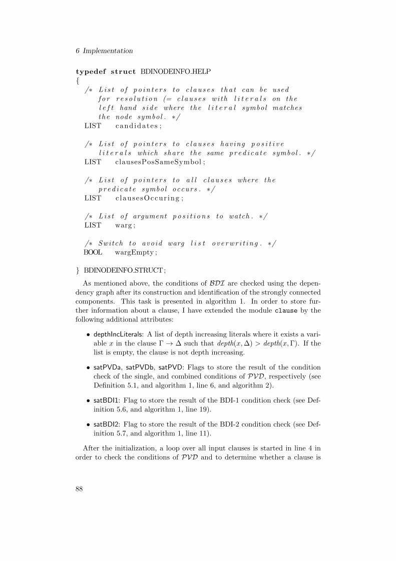
6 Implementation
typedef struct BDINODEINFO HELP{
/∗ L i s t o f p o i n t e r s to c l a u s e s t h a t can be usedf o r r e s o l u t i o n (= c l a u s e s wi th l i t e r a l s on thel e f t hand s i d e where the l i t e r a l symbol matchesthe node symbol . ∗/
LIST cand idates ;
/∗ L i s t o f p o i n t e r s to c l a u s e s having p o s i t i v el i t e r a l s which share the same p r e d i c a t e symbol . ∗/
LIST clausesPosSameSymbol ;
/∗ L i s t o f p o i n t e r s to a l l c l a u s e s where thep r e d i c a t e symbol occurs . ∗/
LIST c lause sOccur ing ;
/∗ L i s t o f argument p o s i t i o n s to watch . ∗/LIST warg ;
/∗ Switch to avoid warg l i s t o v e r w r i t i n g . ∗/BOOL wargEmpty ;
} BDINODEINFO STRUCT;
As mentioned above, the conditions of BDI are checked using the depen-dency graph after its construction and identification of the strongly connectedcomponents. This task is presented in algorithm 1. In order to store fur-ther information about a clause, I have extended the module clause by thefollowing additional attributes:
• depthIncLiterals: A list of depth increasing literals where it exists a vari-able x in the clause Γ → ∆ such that depth(x,∆) > depth(x,Γ). If thelist is empty, the clause is not depth increasing.
• satPVDa, satPVDb, satPVD: Flags to store the result of the conditioncheck of the single, and combined conditions of PVD, respectively (seeDefinition 5.1, and algorithm 1, line 6, and algorithm 2).
• satBDI1: Flag to store the result of the BDI-1 condition check (see Def-inition 5.6, and algorithm 1, line 19).
• satBDI2: Flag to store the result of the BDI-2 condition check (see Def-inition 5.7, and algorithm 1, line 11).
After the initialization, a loop over all input clauses is started in line 4 inorder to check the conditions of PVD and to determine whether a clause is
88
depth increasing or not. Please note that the access of class attributes orproperties is handled in following algorithms using the dot operator, see line 5for the first occurrence. The condition check for PVD is mainly done by thefunction bdi satPVD(), called in line 6, which marks the depth increasingvariables with varDepthIncMark, stamps the depth increasing argument posi-tions of the related literal, and remembers the depth increasing literals of theclause in the list depthIncLiterals of that clause. The result of the check is thenstored in the attribute satPVD of the clause. Of course, if a clause violatesthe single condition satPVDa (PVD-(i), Definition 5.1), it can never satisfy aBDI condition (line 7) because PVD-(i) must hold both for BDI-1 and BDI-2.Otherwise, if only PVD-(ii) is violated, the clause is depth increasing and hasto be stored in line 9 to be considered for checking the conditions of BDI-1,and BDI-2 in the subsequent loops.
The loop to check the BDI-2 conditions starts in line 11, where the functionbdi satBDI2() is actually doing the job: It checks the single BDI-2 conditionsand initializes also the watched argument lists that are needed for the followingBDI-1 condition check. Additionally, it remembers all clauses satisfying BDI-2in order to be able to check BDI-(iv) at the end (line 23).
The subsequent loop (line 16) considers again all depth increasing clauses tocheck the BDI-1 conditions (function bdi satBDI1(), line 19), but only if thecorresponding clause does not already satisfy BDI-2 (line 17). The result ofthe BDI-1 condition check is also stored in the clause, like the previous resultsPVD, and BDI-2.
Eventually, a loop over all depth increasing clauses is started in line 20, inorder to check whether the clause satisfies BDI-1 or BDI-2. If a clause satisfiesBDI-2, all other clauses satisfying BDI-2 have to be checked in a separate loopin line 23 for reachability, because in order to satisfy BDI-(iv), two depthincreasing clauses both satisfying BDI-2 may not reachable from each other.This requirement is implemented by taking the first literal from the respectivedepth increasing literal lists (lines 24-25)1, and check reachability of these twoliterals by means of the graph, if the literals are not equal. The equality isexcluded and can be excluded because it represents the case that the clausesClause and Clause2 are equal and we want to check reachability only for twodifferent clauses Clause and Clause2.
1Please note that there exists only one element in the depth increasing literal list for aclause satisfying BDI-2.
89
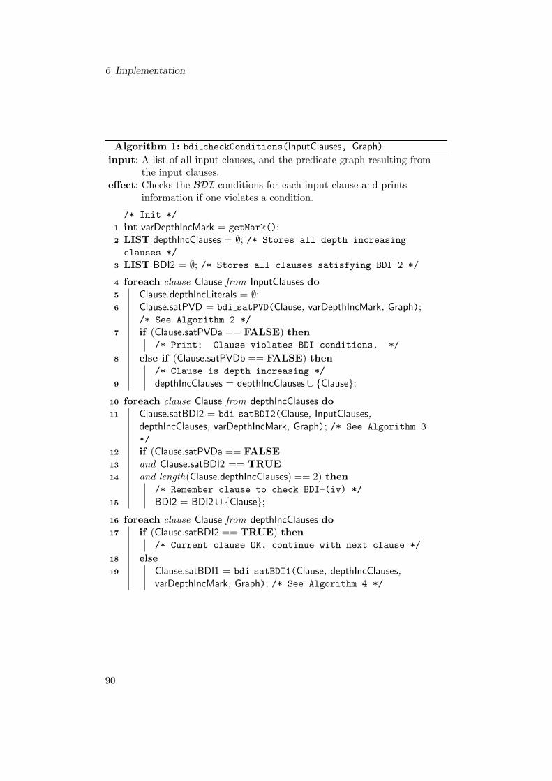
6 Implementation
Algorithm 1: bdi checkConditions(InputClauses, Graph)
input: A list of all input clauses, and the predicate graph resulting fromthe input clauses.
effect: Checks the BDI conditions for each input clause and printsinformation if one violates a condition.
/* Init */
1 int varDepthIncMark = getMark();2 LIST depthIncClauses = ∅; /* Stores all depth increasing
clauses */
3 LIST BDI2 = ∅; /* Stores all clauses satisfying BDI-2 */
4 foreach clause Clause from InputClauses do5 Clause.depthIncLiterals = ∅;6 Clause.satPVD = bdi satPVD(Clause, varDepthIncMark, Graph);
/* See Algorithm 2 */
7 if (Clause.satPVDa == FALSE) then/* Print: Clause violates BDI conditions. */
8 else if (Clause.satPVDb == FALSE) then/* Clause is depth increasing */
9 depthIncClauses = depthIncClauses ∪ {Clause};
10 foreach clause Clause from depthIncClauses do11 Clause.satBDI2 = bdi satBDI2(Clause, InputClauses,
depthIncClauses, varDepthIncMark, Graph); /* See Algorithm 3
*/
12 if (Clause.satPVDa == FALSE13 and Clause.satBDI2 == TRUE14 and length(Clause.depthIncClauses) == 2) then
/* Remember clause to check BDI-(iv) */
15 BDI2 = BDI2 ∪ {Clause};
16 foreach clause Clause from depthIncClauses do17 if (Clause.satBDI2 == TRUE) then
/* Current clause OK, continue with next clause */
18 else19 Clause.satBDI1 = bdi satBDI1(Clause, depthIncClauses,
varDepthIncMark, Graph); /* See Algorithm 4 */
90
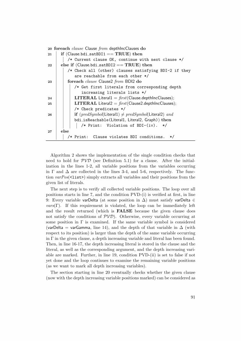
20 foreach clause Clause from depthIncClauses do21 if (Clause.bdi satBDI1 == TRUE) then
/* Current clause OK, continue with next clause */
22 else if (Clause.bdi satBDI2 == TRUE) then/* Check all (other) clauses satisfying BDI-2 if they
are reachable from each other */
23 foreach clause Clause2 from BDI2 do/* Get first literals from corresponding depth
increasing literals lists */
24 LITERAL Literal1 = first(Clause.depthIncClauses);25 LITERAL Literal2 = first(Clause2.depthIncClauses);
/* Check predicates */
26 if (predSymbol(Literal1) 6= predSymbol(Literal2) andbdi isReachable(Literal1, Literal2, Graph)) then
/* Print: Violation of BDI-(iv). */
27 else/* Print: Clause violates BDI conditions. */
Algorithm 2 shows the implementation of the single condition checks thatneed to hold for PVD (see Definition 5.1) for a clause. After the initial-ization in the lines 1-2, all variable positions from the variables occurringin Γ and ∆ are collected in the lines 3-4, and 5-6, respectively. The func-tion varPos(<list>) simply extracts all variables and their positions from thegiven list of literals.
The next step is to verify all collected variable positions. The loop over allpositions starts in line 7, and the condition PVD-(i) is verified at first, in line9: Every variable varDelta (at some position in ∆) must satisfy varDelta ∈vars(Γ). If this requirement is violated, the loop can be immediately leftand the result returned (which is FALSE because the given clause doesnot satisfy the conditions of PVD). Otherwise, every variable occurring atsome position in Γ is examined. If the same variable symbol is considered(varDelta = varGamma, line 14), and the depth of that variable in ∆ (withrespect to its position) is larger than the depth of the same variable occurringin Γ in the given clause, a depth increasing variable and literal has been found.Then, in line 16-17, the depth increasing literal is stored in the clause and theliteral, as well as the corresponding argument, and the depth increasing vari-able are marked. Further, in line 19, condition PVD-(ii) is set to false if notyet done and the loop continues to examine the remaining variable positions(as we want to mark all depth increasing variables).
The section starting in line 20 eventually checks whether the given clause(now with the depth increasing variable positions marked) can be considered as
91

6 Implementation
a candidate to satisfy BDI-2. This is not the case if it has more than one depthincreasing literal for which the graph node information is adjusted by flushingthe watched argument list and setting the flag wargEmpty = TRUE to preventlater overriding of the watched argument list. The idea and implementationof the watched argument list is explained in detail in algorithm 6. The nodeinformation is attached to each predicate symbol and is accessible via thepredicate symbol of the literal.
Algorithm 2: bdi satPVD(Clause, depthIncMark, Graph)
input : A clause, a depth increasing mark, and the predicate graph.effect : Checks the PVD conditions on the given clause.output: Returns true if the clause satisfies PVD, false otherwise.
/* Init */
1 Clause.satPVDa = Clause.satPVDb = TRUE;2 LIST VarPosGamma = VarPosDelta = ∅;/* Collect variable positions in Γ */
3 foreach VarPos from varPos(Γ) of Clause do4 VarPosGamma = VarPosGamma ∪ {VarPos};
/* Collect variable positions in ∆ */
5 foreach VarPos from varPos(∆) of Clause do6 VarPosDelta = VarPosDelta ∪ {VarPos};
7 foreach VarPosFromDelta ∈ VarPosDelta do /* Check variables at
the positions */
8 SYMBOL varDelta = getVarAtPos(VarPosFromDelta);9 if (varDelta /∈ vars(Γ)) then
10 Clause.satPVDa = FALSE;/* Print: Clause violates PVD-(i). */
11 break;
12 foreach VarPosFromGamma ∈ VarPosGamma do13 SYMBOL varGamma = getVarAtPos(VarPosFromGamma);14 if (varDelta == varGamma and
depth(VarPosFromDelta,∆) > depth(VarPosFromGamma,Γ))then
15 Clause.depthIncLiterals = Clause.depthIncLiterals∪ {getLiteral(VarPosFromDelta)};
16 Stamp depth increasing argument of literal and literal itself;17 Mark depth increasing variable (position) with
depthIncMark;
92

18 if (Clause.satPVDb == TRUE) then19 Clause.satPVDb = FALSE;
/* Print: Clause violates PVD-(ii). */
/* Continue with other depth increasing vars */
20 if (length(Clause.depthIncLiterals) > 1) then/* Clause can never satisfy BDI-2, possibly BDI-1;
adjust graph node info for all literals from
depthIncLiterals */
21 foreach Literal from depthIncLiterals do22 GRAPHNODE Node = getNode(Literal);23 Node.nodeInfo.warg = ∅;24 Node.nodeInfo.wargEmpty = TRUE;
25 return (Clause.satPVDa and Clause.satPVDb);
The algorithm 3 shows the implementation of the single condition checks forBDI-2 as well as the initialization of the watched argument list for the predi-cates. After the initialization in the lines 1-3, the attribute PVDa (conditionPVD-(i)) is checked for the given clause in lines 5-6 because it is a requirementfor BDI-2, too. The PVDa attribute has been previously set in algorithm 2which is executed prior to the current algorithm. Afterwards, the number ofdepth increasing literals in the depth increasing literal list of the given clauseis verified to be exactly one in the lines 7-8. If these preconditions are satisfied,the actual examination of the positive literals of the clause starts in line 9. Inlines 12-13 it is checked for every stamped (depth increasing) literal whetherthe depth increasing argument position(s) of the given literal are the same forall positive literal occurrences with the same predicate symbol in the otherinput clauses. Please note that the corresponding clauses sharing the samepredicate symbol have been stored during the graph construction in the listclausesPosSameSymbol to avoid repeated loops over all input clauses.
The next part is the check of the number of depth increasing arguments aswell as to determine the watched argument positions for the depth increasingliteral and the reachable literals in the same cycle. For this purpose, a loopover all arguments of the depth increasing literal is necessary (starting inline 16) where the number of marked arguments is verified at first in line 20.Further, the depth increasing literal and argument position is stored for lateruse in the lines 22-23. If the argument is not marked and therefore not depthincreasing, its position is stored in the watched argument list that is kept inthe additional information of the literals graph node (line 25).
The call of the function bdi setWargReachable() in line 26 passes thewatched argument list to all literals occurring in the same cycle than thecurrent depth increasing literal. Please note that the watched argument list
93

6 Implementation
gets only passed to those literals having the wargEmpty flag not set, otherwisethe watched argument list of the corresponding literal remains unchanged. Adetailed explanation of the watched arguments and their implementation isgiven in the context of Algorithm 6.
The next part is the exploration of the negative literals of the given clause inthe loop starting in line 27). For all atoms that are reachable from the depthincreasing literal with common variables (line 29), the conditions of BDI-2-(iii)have to be checked: The arity of the negative literal and the depth increasingliteral must be equal (BDI-2-(iii)-(1), lines 30-31), the respective watched ar-guments must be equal (BDI-2-(iii)-(2), lines 32-33), and the depth increasingargument and the negative literal are not allowed to have common variables(BDI-2-(iii)-(3), lines 34-35). Afterwards, the variables are collected for thelater check of condition BDI-2-(v), either only from the arguments at watchedargument positions if the literal is reachable from a depth increasing clause(lines 36-37), or by taking all variables from the literal otherwise (lines 38-39).
In order to check BDI-2-(iv), it’s necessary to scan all clauses in the samecycle or component than the given clause for a literal that is reachable fromthe current depth increasing literal. For the matching clauses, we require forany literal in the succedent with a non-empty watched argument list that thewatched argument list for all atoms in the antecedent is either identical orempty (checked by wargEmptyOrEqual() in line 42). The function stops andreturns FALSE if this requirement is violated.
Finally, another loop over all positive literals of the given clause is performedto check the condition BDI-2-(v) in the lines 44-46. This separate loop isneeded because its contents can’t be moved to the first loop over the succedentof the clause (in line 9) due to dependencies. The reason is the necessarycollection of the corresponding variables that only takes place in the loop overthe negative literals of the given clause (starting in line 27) and which inturn needs to be executed after a loop over the positive literals (also becauseof dependencies). If a literal different from the depth increasing literal isencountered and the variables of the non-depth-increasing literal are not inthe list of allowed variables (line 45), then the condition BDI-2-(v) is violated.
If none of the previous checks has failed, the given clause satisfies BDI-2and the function sat BDI2() returns TRUE in line 47.
94

Algorithm 3: bdi satBDI2(Clause, depthIncClauses, depthIncMark,Graph)
input : A clause, the list of depth increasing clauses, a depth increasingmark, and the predicate graph.
effect : Checks the BDI-2 conditions on the given clause.output: Returns true if the clause satisfies BDI-2, false otherwise.
/* Init */
1 LITERAL depthIncLiteral = NULL;2 int depthIncArgPos = 0;3 LIST allowedVars = ∅;4 GRAPHNODE Node;
5 if (Clause.satPVDa == FALSE) then6 return FALSE;
7 if (length(Clause.depthIncLiterals) > 1) then8 return FALSE ; /* Print: More than 1 depth increasing
literal */
9 foreach Literal ∈ ∆ of Clause do10 if (Literal is stamped) then11 Node = getNode(Literal);12 if (bdi isUniquelyDepthInc(Literal,
Node.nodeInfo.clausesPosSameSymbol) == FALSE) then/* See Algorithm 5 */
13 return FALSE; /* Not uniquely depth increasing */
/* Init search for depth increasing literal and
argument */
14 countDephIncArgs = 0;15 argPos = 0;16 foreach Argument ∈ Literal do17 argPos++;18 if (Argument is marked) then19 countDephIncArgs++;20 if (countDephIncArgs > 1) then
/* Print: > 1 depth increasing argument */
21 return FALSE;
22 depthIncLiteral = Literal; /* Remember literal and
argument position */
23 depthIncArgPos = argPos;
24 else25 Node.nodeInfo.warg = Node.nodeInfo.warg ∪ {argPos};26 bdi setWargReachable(Literal,Graph); /* See Algorithm 6
*/
95

6 Implementation
27 foreach Literal ∈ Γ of Clause do28 Node = getNode(Literal);29 if (bdi isReachable(Literal, depthIncLiteral,Graph) and
vars(Literal) ∩ vars(depthIncLiteral) 6= ∅) then/* BDI-2-(iii)-(1), see Algorithm 7 */
30 if arity(Literal) 6= arity(depthIncLiteral) then31 return FALSE /* Print: arities not equal */
32 else if (wargEqual(Node.nodeInfo.warg,getNode(depthIncLiteral).nodeInfo.warg) == FALSE) then/* BDI-2-(iii)-(2) */
33 return FALSE ; /* Print: warg lists not equal */
34 else if (vars(Literal) ∩vars(getArgument(depthIncLiteral, depthIncArgPos)) 6= ∅) then/* BDI-2-(iii)-(3) */
/* Print: Violation of BDI-2-(iii)-(3) */
35 return FALSE;
/* Collect vars for BDI-2-(v) */
36 if (bdi isReachableFromDIC(Literal, depthIncClauses,Graph)) then/* Reachable from DIC, only vars from warg list; see
Algorithm 8 */
37 allowedVars = allowedVars ∪ vars(Node.nodeInfo.warg);
38 else /* Not reachable from DIC, take all vars */
39 allowedVars = allowedVars ∪ vars(Literal);
40 foreach clause Clause2 in same cycle than Clause do /* BDI-2-(iv)
*/
41 foreach Literal ∈ ∆ of Clause2 do42 if (bdi isReachable(Literal, depthIncLiteral,Graph)) and
wargEmptyOrEqual(Clause2,Graph) == FALSE then /* See
Algorithm 9 */
43 return FALSE ; /* Print: BDI-2-(iv) violated. */
44 foreach Literal ∈ ∆ of Clause do /* BDI-2-(v) */
45 if (Literal 6= depthIncLiteral and vars(Literal) ∩ allowedVars == ∅)then
46 return FALSE ; /* Print: BDI-2-(v) violated. */
47 return TRUE;
96
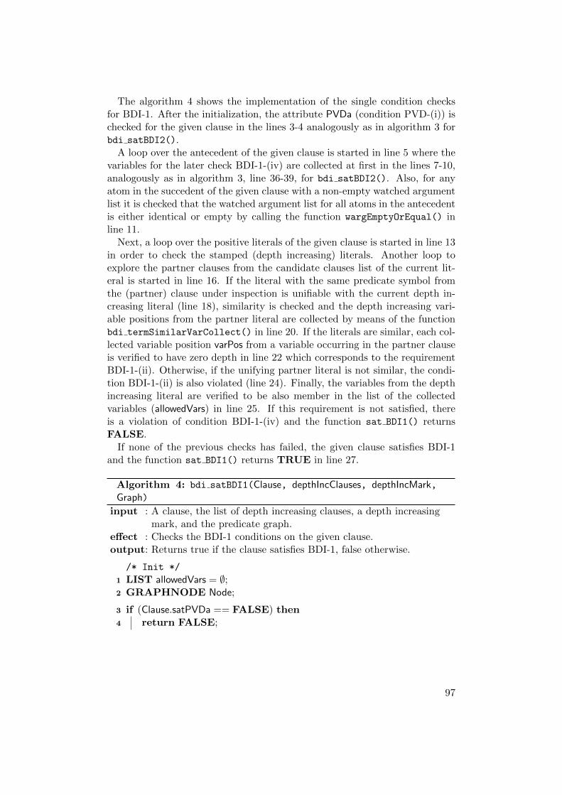
The algorithm 4 shows the implementation of the single condition checksfor BDI-1. After the initialization, the attribute PVDa (condition PVD-(i)) ischecked for the given clause in the lines 3-4 analogously as in algorithm 3 forbdi satBDI2().
A loop over the antecedent of the given clause is started in line 5 where thevariables for the later check BDI-1-(iv) are collected at first in the lines 7-10,analogously as in algorithm 3, line 36-39, for bdi satBDI2(). Also, for anyatom in the succedent of the given clause with a non-empty watched argumentlist it is checked that the watched argument list for all atoms in the antecedentis either identical or empty by calling the function wargEmptyOrEqual() inline 11.
Next, a loop over the positive literals of the given clause is started in line 13in order to check the stamped (depth increasing) literals. Another loop toexplore the partner clauses from the candidate clauses list of the current lit-eral is started in line 16. If the literal with the same predicate symbol fromthe (partner) clause under inspection is unifiable with the current depth in-creasing literal (line 18), similarity is checked and the depth increasing vari-able positions from the partner literal are collected by means of the functionbdi termSimilarVarCollect() in line 20. If the literals are similar, each col-lected variable position varPos from a variable occurring in the partner clauseis verified to have zero depth in line 22 which corresponds to the requirementBDI-1-(ii). Otherwise, if the unifying partner literal is not similar, the condi-tion BDI-1-(ii) is also violated (line 24). Finally, the variables from the depthincreasing literal are verified to be also member in the list of the collectedvariables (allowedVars) in line 25. If this requirement is not satisfied, thereis a violation of condition BDI-1-(iv) and the function sat BDI1() returnsFALSE.
If none of the previous checks has failed, the given clause satisfies BDI-1and the function sat BDI1() returns TRUE in line 27.
Algorithm 4: bdi satBDI1(Clause, depthIncClauses, depthIncMark,Graph)
input : A clause, the list of depth increasing clauses, a depth increasingmark, and the predicate graph.
effect : Checks the BDI-1 conditions on the given clause.output: Returns true if the clause satisfies BDI-1, false otherwise.
/* Init */
1 LIST allowedVars = ∅;2 GRAPHNODE Node;
3 if (Clause.satPVDa == FALSE) then4 return FALSE;
97

6 Implementation
5 foreach Literal ∈ Γ of Clause do6 Node = getNode(Literal);
/* Collect vars for BDI-1-(iv) */
7 if (bdi isReachableFromDIC(Literal, depthIncClauses,Graph)) then/* Reachable from DIC, take only variables from warg
list, see Algorithm 8 */
8 allowedVars = allowedVars ∪ vars(Node.nodeInfo.warg);
9 else /* Not reachable from DIC, take all variables */
10 allowedVars = allowedVars ∪ vars(Literal);11 if (wargEmptyOrEqual(Clause,Graph) == FALSE) then /* See
Algorithm 9 */
/* Print: Violation of BDI-1-(v). */
12 return FALSE;
13 foreach Literal ∈ ∆ of Clause do14 Node = getNode(Literal);15 if (Literal is stamped) then16 foreach partner clause Clause2 ∈ Node.nodeInfo.candidates do
/* Examine resolution partners */
17 foreach literal with same predicate symbolLiteral2 ∈ Clause2 do
18 if (isUnifiable(Literal, Literal2)) then19 LIST varPosCheck = ∅;
/* Check similarity and collect depth
increasing variables in partner literal
*/
20 if (bdi termSimilarVarCollect(Literal, Literal2,varDepthIncMark, varPosCheck)) then /* See
algorithm 10 */
21 foreach varPos ∈ varPosCheck do /* Verify
variable positions */
22 if (depth(varPos,Clause2) > 0) then/* Print: Violation of BDI-1-(ii)
*/
23 return FALSE;
24 else/* Print: Violation of BDI-1-(ii),
literal in partner clause is not
similar */
/* Check vars (collected previously) */
25 if (vars(Literal) ∩ allowedVars == ∅) then/* Print: Violation of BDI-1-(iv). */
26 return FALSE;
27 return TRUE;
98
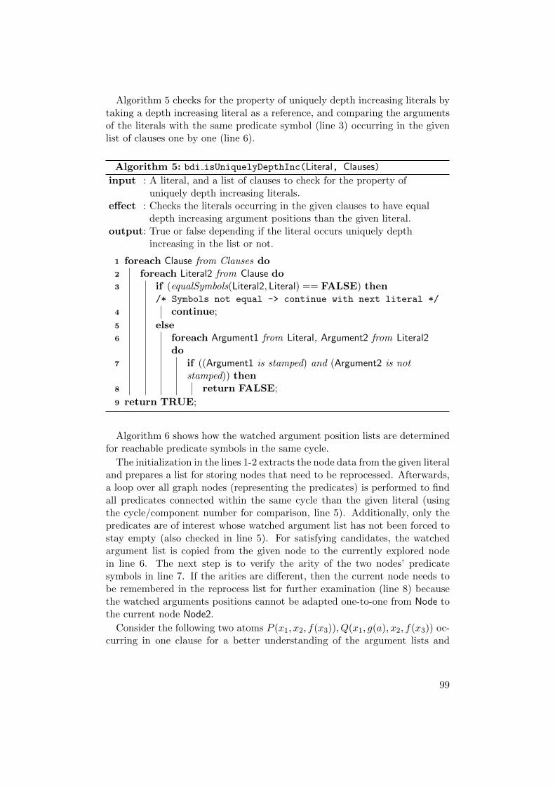
Algorithm 5 checks for the property of uniquely depth increasing literals bytaking a depth increasing literal as a reference, and comparing the argumentsof the literals with the same predicate symbol (line 3) occurring in the givenlist of clauses one by one (line 6).
Algorithm 5: bdi isUniquelyDepthInc(Literal, Clauses)
input : A literal, and a list of clauses to check for the property ofuniquely depth increasing literals.
effect : Checks the literals occurring in the given clauses to have equaldepth increasing argument positions than the given literal.
output: True or false depending if the literal occurs uniquely depthincreasing in the list or not.
1 foreach Clause from Clauses do2 foreach Literal2 from Clause do3 if (equalSymbols(Literal2, Literal) == FALSE) then
/* Symbols not equal -> continue with next literal */
4 continue;
5 else6 foreach Argument1 from Literal, Argument2 from Literal2
do7 if ((Argument1 is stamped) and (Argument2 is not
stamped)) then8 return FALSE;
9 return TRUE;
Algorithm 6 shows how the watched argument position lists are determinedfor reachable predicate symbols in the same cycle.
The initialization in the lines 1-2 extracts the node data from the given literaland prepares a list for storing nodes that need to be reprocessed. Afterwards,a loop over all graph nodes (representing the predicates) is performed to findall predicates connected within the same cycle than the given literal (usingthe cycle/component number for comparison, line 5). Additionally, only thepredicates are of interest whose watched argument list has not been forced tostay empty (also checked in line 5). For satisfying candidates, the watchedargument list is copied from the given node to the currently explored nodein line 6. The next step is to verify the arity of the two nodes’ predicatesymbols in line 7. If the arities are different, then the current node needs tobe remembered in the reprocess list for further examination (line 8) becausethe watched arguments positions cannot be adapted one-to-one from Node tothe current node Node2.
Consider the following two atoms P (x1, x2, f(x3)), Q(x1, g(a), x2, f(x3)) oc-curring in one clause for a better understanding of the argument lists and
99

6 Implementation
assume that the argument positions 1 = x1, 2 = x2 for P are watched. Asmentioned above, the watched argument list of P (positions 1, 2) is initiallycopied to the watched argument lists of all other reachable predicates in thesame cycle (in this example on the predicate Q). However, one easily can seethat the (watched) argument positions 1, 2 of P are identical to the arguments1, 3 of Q. Hence, the initially copied watched argument positions 1, 2 for Q arewrong and need to be fixed. The correction is done by identifying the samearguments and their corresponding positions between two atoms in the sameclause even if there are other arguments in between. The only requirement isthat the arguments stay sorted. It is not permitted to swap positions, e.g.,to have the argument position of x2 before the argument position of x1 inQ. In our example, the argument in between in Q(x1, g(a), x2, f(x3)) is g(a)that causes an update of the initially watched argument positions for Q, i.e.,positions 1, 3 instead of 1, 2.
The examination of the arguments, detection of the correct positions forpredicates with a different arity and the subsequent update of the wrong po-sitions is done in the loop over the remembered nodes from the reprocess liststarting in line 9. For every remembered node that has already a (possiblywrong) watched argument list, all appropriate clauses (loop starting in line 10)and literals (lines 13-22) are searched to use as source (from where the watchedargument positions are read from) and target (where the watched argumentshave to be updated). For any found pair of source and target literal (line 23),the mapping process between the arguments of source and target literal is per-formed (starting in line 25). As illustrated in the previous example for P andQ, the arguments from the source literal at the given watched argument po-sition of Node are read and the corresponding (same) arguments are searchedin the target literal. The new watched argument positions in the target literalare preliminary temporary and stored in the list wargTargTmp (line 28). Af-terwards, after a verification of the correct length (line 29) by comparing thetemporary list with the current (possibly still wrong) watched argument listof the given node, the temporary list is assigned as the new watched argumentlist to the given node (line 30), and the loop continues with the next predicateto review (line 31). Otherwise, if the length of the new watched argument listdiffers from the length of the existing list, the old watched argument list iskept for the predicate.
100

Algorithm 6: bdi setWargReachable(Literal, Graph)
input : A literal, and the predicate graph of the input clauses.effect : Searches all connected nodes (predicates) in the same component
and copies the watched argument list to the connected nodeunless the connected node has been forced to stay empty forsome reason (flag wargEmpty).
output: Nothing.
/* Init */
1 GRAPHNODE Node = getNode(Literal);2 LIST ReprocessList = ∅;3 LIST GraphNodes = getGraphNodes(Graph);
4 foreach Node2 from GraphNodes do /* Search all connected
predicates in the same component */
5 if ((Node2.compNumber == Node.compNumber) and(Node2.wargEmpty == FALSE)) then /* Same
component/reachable, and watched argument position list
is not forced to stay empty -> copy watched argument
position list to reachable node */
6 Node2.nodeInfo.warg = Node.nodeInfo.warg;7 if (arity(Node2.symbol) 6= arity(Node.symbol)) then /* Arity
different -> remember node to update warg list after
further examination */
8 ReprocessList = ReprocessList ∪ {Node2};9 foreach Node2 from ReprocessList do
10 foreach Clause from Node2.clausesOccurring do /* Search for a
clause having a literal with the current symbol */
11 LITERAL LiteralSrc = NULL;12 LITERAL LiteralTarg = NULL;13 foreach Literal2 ∈ Clause do /* Examine literals */
14 GRAPHNODE Node3 = getNode(Literal2);15 if ((LiteralSrc 6= NULL) and (LiteralTarg 6= NULL)) then
/* Literals found, stop search */
16 break;17 if (Node3.nodeInfo.warg == ∅) then /* warg list must
be non-empty, continue search */
18 continue;19 if (arity(Node3.symbol)) == arity(Node.symbol)) then20 LiteralSrc = Literal2;21 else22 LiteralTarg = Literal2;
101
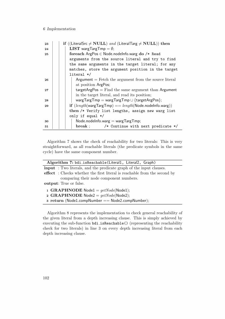
6 Implementation
23 if ((LiteralSrc 6= NULL) and (LiteralTarg 6= NULL)) then24 LIST wargTargTmp = ∅;25 foreach ArgPos ∈ Node.nodeInfo.warg do /* Read
arguments from the source literal and try to find
the same arguments in the target literal; for any
matches, store the argument position in the target
literal */
26 Argument = Fetch the argument from the source literalat position ArgPos;
27 targetArgPos = Find the same argument than Argumentin the target literal, and read its position;
28 wargTargTmp = wargTargTmp ∪ {targetArgPos};29 if (length(wargTargTmp) == length(Node.nodeInfo.warg))
then /* Verify list lengths, assign new warg list
only if equal */
30 Node.nodeInfo.warg = wargTargTmp;31 break ; /* Continue with next predicate */
Algorithm 7 shows the check of reachability for two literals: This is verystraightforward, as all reachable literals (the predicate symbols in the samecycle) have the same component number.
Algorithm 7: bdi isReachable(Literal1, Literal2, Graph)
input : Two literals, and the predicate graph of the input clauses.effect : Checks whether the first literal is reachable from the second by
comparing their node component numbers.output: True or false.
1 GRAPHNODE Node1 = getNode(Node1);2 GRAPHNODE Node2 = getNode(Node2);3 return (Node1.compNumber == Node2.compNumber);
Algorithm 8 represents the implementation to check general reachability ofthe given literal from a depth increasing clause. This is simply achieved byexecuting the sub-function bdi isReachable() (representing the reachabilitycheck for two literals) in line 3 on every depth increasing literal from eachdepth increasing clause.
102
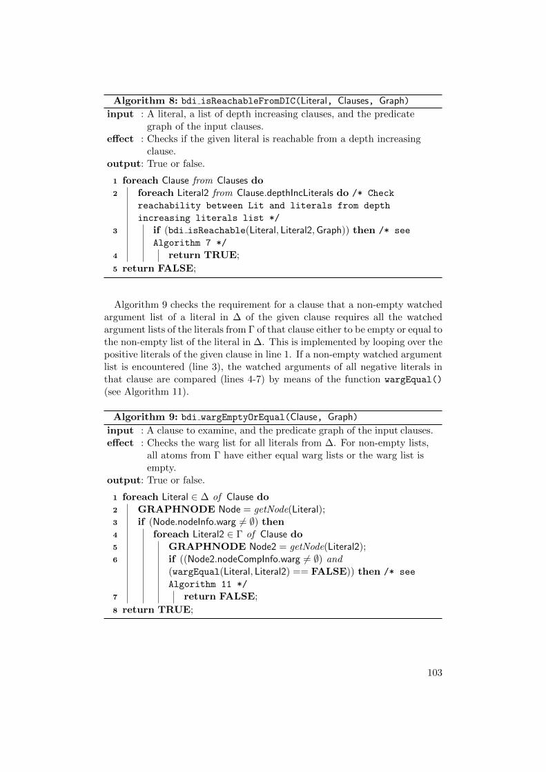
Algorithm 8: bdi isReachableFromDIC(Literal, Clauses, Graph)
input : A literal, a list of depth increasing clauses, and the predicategraph of the input clauses.
effect : Checks if the given literal is reachable from a depth increasingclause.
output: True or false.
1 foreach Clause from Clauses do2 foreach Literal2 from Clause.depthIncLiterals do /* Check
reachability between Lit and literals from depth
increasing literals list */
3 if (bdi isReachable(Literal, Literal2,Graph)) then /* see
Algorithm 7 */
4 return TRUE;
5 return FALSE;
Algorithm 9 checks the requirement for a clause that a non-empty watchedargument list of a literal in ∆ of the given clause requires all the watchedargument lists of the literals from Γ of that clause either to be empty or equal tothe non-empty list of the literal in ∆. This is implemented by looping over thepositive literals of the given clause in line 1. If a non-empty watched argumentlist is encountered (line 3), the watched arguments of all negative literals inthat clause are compared (lines 4-7) by means of the function wargEqual()
(see Algorithm 11).
Algorithm 9: bdi wargEmptyOrEqual(Clause, Graph)
input : A clause to examine, and the predicate graph of the input clauses.effect : Checks the warg list for all literals from ∆. For non-empty lists,
all atoms from Γ have either equal warg lists or the warg list isempty.
output: True or false.
1 foreach Literal ∈ ∆ of Clause do2 GRAPHNODE Node = getNode(Literal);3 if (Node.nodeInfo.warg 6= ∅) then4 foreach Literal2 ∈ Γ of Clause do5 GRAPHNODE Node2 = getNode(Literal2);6 if ((Node2.nodeCompInfo.warg 6= ∅) and
(wargEqual(Literal, Literal2) == FALSE)) then /* see
Algorithm 11 */
7 return FALSE;
8 return TRUE;
103

6 Implementation
Algorithm 10 is a recursive function used to check the similarity of twogiven terms by traversing the tree representations of the terms. Additionally,the function collects the variables from the compared term (Term2) that aresubject to further checks (which have to be carried out separately, see Algo-rithm 4, line 21). For storing the variables, a pointer to a list object (varcheck)is passed to the function such that the list is still available after leaving thefunction. The function traverses the tree representation of the terms one byone and subsequently examines the single components. The beginning in line 1checks for equal terms which are trivially similar. Contrary, if two terms havedifferent (top) symbols (checked in line 3), they can never be similar and thealgorithms immediately stops by returning FALSE. Otherwise, the argumentsof the two given terms are explored using a loop. In case of having a variableas the first (argument) term and a constant as the second (argument) term(line 7), the terms are similar but there are no variables to collect. Otherwise,if there is a variable or constant as the first term, and a variable as the sec-ond term (line 9), the first term is checked to be depth increasing (it is thenmarked with the depth increasing mark depthIncMark). If the depth increas-ing condition is satisfied, the second term (which is a variable) is then storedin the list varcheck in line 11. For the case of neither having variables norconstants, the present terms must be functional for which we go into recursionwith the arguments in line 13 (and such traversing the tree). Eventually, inline 16, the function bdi termSimilarVarCollect() returns TRUE if bothargument lists of a function have been processed one by one and no argumentis left, and FALSE otherwise.
The following examples depict the working principle of the previously de-scribed algorithm. Consider the terms f(g(x)) and f(g(a)) where x is a vari-able, and a a constant. For this input, the function symbols f and g arerecursively examined to be equal one by one, and then on the most deeplyargument level, the case in line 7 is entered with the terms Argument1 = xand Argument2 = a, respectively.
Another example are the terms f(g(x)), f(g(y)). Let’s assume that thevariable x in the first term has been marked to be depth increasing. Then,after two recursion steps for examining the function symbols f and g, the casein line 9 is entered for the variables and the variable y is then collected becausex at the same tree position than y has been marked to be depth increasing.
104
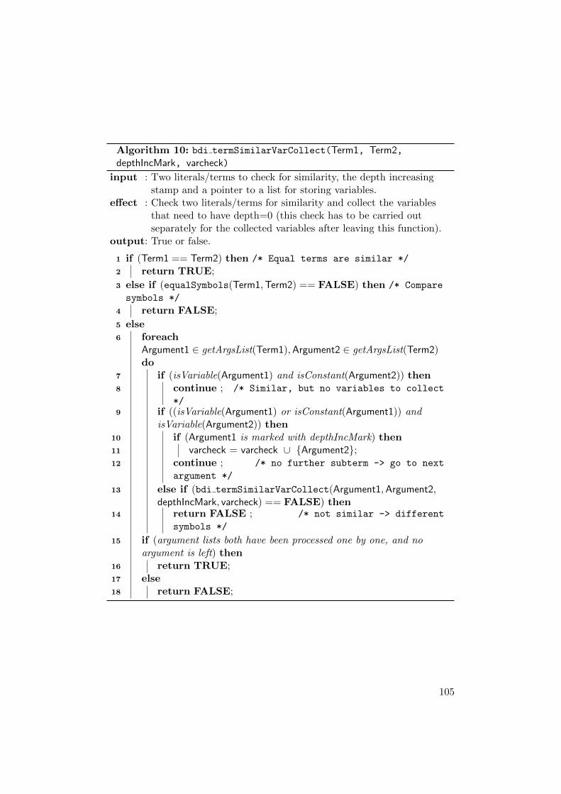
Algorithm 10: bdi termSimilarVarCollect(Term1, Term2,depthIncMark, varcheck)
input : Two literals/terms to check for similarity, the depth increasingstamp and a pointer to a list for storing variables.
effect : Check two literals/terms for similarity and collect the variablesthat need to have depth=0 (this check has to be carried outseparately for the collected variables after leaving this function).
output: True or false.
1 if (Term1 == Term2) then /* Equal terms are similar */
2 return TRUE;
3 else if (equalSymbols(Term1,Term2) == FALSE) then /* Compare
symbols */
4 return FALSE;
5 else6 foreach
Argument1 ∈ getArgsList(Term1),Argument2 ∈ getArgsList(Term2)do
7 if (isVariable(Argument1) and isConstant(Argument2)) then8 continue ; /* Similar, but no variables to collect
*/9 if ((isVariable(Argument1) or isConstant(Argument1)) and
isVariable(Argument2)) then10 if (Argument1 is marked with depthIncMark) then11 varcheck = varcheck ∪ {Argument2};12 continue ; /* no further subterm -> go to next
argument */
13 else if (bdi termSimilarVarCollect(Argument1,Argument2,depthIncMark, varcheck) == FALSE) then
14 return FALSE ; /* not similar -> different
symbols */
15 if (argument lists both have been processed one by one, and noargument is left) then
16 return TRUE;17 else18 return FALSE;
105

6 Implementation
Algorithm 11 shows the implementation of the comparison between thewatched argument lists of two literals. After the initialization in the lines 1-2,the length of the two literals’ watched argument lists is compared at first inline 3. In order to be equal, also the number of watched arguments must beequal. In line 5 starts a loop for the pairwise comparison of the argument po-sitions. At first, in line 6, it is verified whether the stored watched argumentposition is in fact an admissible argument position available for the presentliteral. Second, in line 8, the actual arguments referenced by their positionsare read and compared to each other.
Algorithm 11: bdi wargEqual(Literal1, Literal2)
input : Two literals.effect : Verifies whether the arguments from the given literals that are
specified by their corresponding watched argument lists, aresimilar (pairwise position checking).
output: True or false.
1 GRAPHNODE Node1 = getNode(Literal1);2 GRAPHNODE Node2 = getNode(Literal2);3 if (length(Node1.nodeInfo.warg) 6= length(Node2.nodeInfo.warg)) then4 return FALSE;
5 foreachArgPos1 ∈ Node1.nodeInfo.warg,ArgPos2 ∈ Node2.nodeInfo.warg do/* Check watched arguments */
/* 1. Check argument positions */
6 if ((ArgPos1 > length(getArgsList(Literal1))) or(ArgPos2 > length(getArgsList(Literal2)))) then
7 return FALSE;
/* 2. Check arguments */
8 if (getArg(Literal1,ArgPos1) 6= getArg(Literal2,ArgPos2)) then9 return FALSE;
10 return TRUE;
106

7 Solving SAP AuthorizationProblems with BDI
The process of solving SAP authorization problems in first-order logic is gen-erally the following: First, the problem needs to be decidable. This is easy ifthe problem (usually identified by its clausal structure) belongs to a knowndecidable class, i.e., all clauses satisfy the properties of the class. However, ifthere are (some) clauses violating these properties, it is maybe still possible toestablish satisfiability by transforming and rewriting the violating candidatessuch that they become conform with the decidable class requirements after-wards. The last step in the solving process is eventually the application of the(problem) solving strategy which exists for all decidable classes.
Applying this process to the SAP authorization problems, the first step isthe identification of the problem structure with respect to decidability. For-tunately, the SAP authorization problems have served as a base to developthe BDI class properties (Chapter 5), and thus, almost all clauses of theseproblems already satisfy the BDI requirements. The BDI properties checkon a problem (instance) is carried out automatically with the theorem proverSpass including the extension described in Chapter 6. As a result of the check,the program outputs affected clauses violating the BDI criteria and additionalinformation about the violated property for the respective clause.
The following clause represents the situation that the authorization valueSTAR matches every other required authorization value, denoted by the variablexav.
∀ xu, xaon, xaof, xav .UserProfile(userProfileEntry(xu, authObj(xaon, xaof, STAR)))
→ Access(xu, authObj(xaon, xaof, xav))
It violates the variable subset property of PVD, BDI-1 (i), BDI-2 (i) and thusBDI. The fulfillment of the BDI requirements is achieved in this example byadding an additional monadic atom ¬Authorization(xav) to the formula anda definition of the admissible constants for the predicate Authorization thatcan be substituted for the variable xav which doesn’t change the meaning ofthe original formula.
Finally, if the (potentially modified) problem (instance) satisfies the BDIrequirements, the solving strategy is applied to the problem. In the contextof my SAP authorization experiments, I have used Hyper-Resolution withFactoring as the decision procedure to deal with the SAP example problems.
107

7 Solving SAP Authorization Problems with BDI
However, Ordered Resolution together with the two additional reduction rulesmaking Ordered Resolution terminating (Section 5.4) should be used for largerreal-world SAP authorization system instances because it is a more efficientand general decision procedure.
In practice, I have utilized the theorem prover Spass with Hyper-Resolutionand Factoring on a server equipped with an Intel Xeon Quad Core X5460 CPUrunning at 3.16GHz, and 16 GB RAM.
I examined several SAP problem variants, all representing the formaliza-tion of the purchase process and typical real-world authorization setups forthis process. The input problems differ in the number of users with (a) 500users and (b) 5.000 users and the users also have different combinations of au-thorization values assigned using single and composite roles. Further, I havechecked the business policies SoD and the four-eyes principle (Section 3.4) onthe purchase process and the authorization setup.
The input file (a) with 500 users could be saturated in less than 1 secondwhile the larger number of users in the input file (b) with 5.000 users (butwith similar authorizations) increased the runtime to 1m34.795s.
The runtime results for the policy checks are similar: A violation of thefour-eyes principle for an input file with 500 users could be detected in 1.033sand a similar policy check with 5.000 users results in a runtime of 1m44.318s.Also, it doesn’t matter how many violations exist: A deliberate manipulationof the input problem to obtain more than one violation of a business policyyields a runtime of 1m44.472s which is almost identical to the run with onlyone violation. This is actually an obvious result because in all cases wherethe input problem is contradictory, Spass outputs a proof and shows thecorresponding parts leading only to the first contradiction – no matter howmany other contradictions exist. In order to detect all contradictions, it isnecessary to fix the contradictory setup and to reapply Spass to find furtherbusiness policy violations. In such cases, one could imagine to implement areuse of an already saturated subset of the input problem for gain a speedup.
108

8 Application to the TPTP Library
The automated theorem prover Spass including the extension described inChapter 6 has been applied to the problems of the TPTP Library, Version6.1.0 [33] in order to detect potential new decidable problems and to findknown undecidable problems “close” to the BDI class that may have only afew clauses responsible for the overall non-termination of the problem.
The current version 6.1.0 of the TPTP Library contains 21.172 problems.Our analysis of the problems ran on the Max Planck Institute’s own servercluster. It consists of 128 Dell PowerEdge M610 Blade Servers, each with2x Intel Xeon Quad Core E5620 running at 2.40 GHz, and 48 GB RAM. Aninternal script provided by the Information Services & Technology department(IST) of the Max Planck Institute is available which takes care of schedulingand submitting jobs to the cluster.
I have written a separate bash shell script for preprocessing that is called bythe job scheduling script in place of directly calling Spass on every problemfrom the library. The preprocessing is used to rule out problems containingequality (because BDI does not deal with equality), as well as problems ex-ceeding a size of more than 3 MB (the total size is calculated from the problemfile itself and potentially included axiom files). If the problem satisfies the pre-vious requirements, the extended version of Spass is called by the shell scriptwith the originally provided arguments. These arguments are in our case:
• -Loops=0Stop after one main loop because we are only interested in analysis ofthe problem and we do not want to saturate it.
• -timelimit=3600A time limit of 3600 seconds per problem that is added in addition to-Loops=0 to prevent excessive input parsing. Sometimes, reading theproblem file and building its clausal form by means of the integratedtool Flotter inside Spass took a very long time.
• -CNFRenaming=0This option causes the formulas not to be equivalently rewritten duringproof search which is sometimes a benefit. Rewriting is not necessarybecause we do only problem analysis which doesn’t need a saturation ofthe input.
• -PGivenPrint the input formula as output.
109
8 Application to the TPTP Library
During every run, the modified program Spass outputs violations of theBDI conditions for any affected clause.
Afterwards, the job scheduling script calls a program “analyzer” whichparses the Spass output using regular expressions and writes the result(s)into a MySQL database. In our case, we are interested in the total numberof clauses for a problem, to count all clauses violating any of the BDI con-ditions and additionally to count the clauses violating only BDI-1 or BDI-2conditions. Of course, the problem name, its rating (specifying the difficultywith respect to ATP) and some other not important values at this place arealso written into the database1.
Having this data available in a database table provides an easy way forquerying. For example, I have identified a total number of 21 undecidableproblems “close” to the BDI class, with a rating > 0, having at least 5 clauses,and where only 1-4 clauses from the set of all clauses violate the BDI-1/BDI-2 conditions (trivial violations due to the variable condition of PVD havebeen ignored). The following Table 8 lists this query result. These problemsmay be altered without much effort into equivalent but decidable problems byreplacing or rewriting the BDI violating clauses.
Another interesting question is to determine the native core for the class,i.e., how many problems from the TPTP Library directly satisfy the BDIrequirements as they are provided – without modification or preprocessing:The result is a total number of 418 clauses.
In total there are 1.402 problems having up to 5 clauses violating the BDIrequirements from which 1.221 problems contradict only the PVD conditions(PVD is included in BDI). Consequently, 181 problems contradicting BDI-1/-2 properties remain. Further requiring a non-empty rating for the 181problems reduces the number to 42.
The last query selects all problems where up to 50% of the clauses of therespective problem may violate the BDI requirements: It yields a total numberof 2.950 problems.
1The analyzer script is a general tool also used by other people and therefore collects awhole bunch of data from the Spass output. It has been extended to collect the dataspecific to the BDI class
110

Problem Rating Number ofClauses
ViolatingBDI
Violatingonly BDI-1/-2
SYN311-1 0.17 6 2 2
MSC013+1 0.56 11 1 1
MSC014+1 0.4 9 1 1
SET830-2 0.22 10 3 2
NUM284-1.014 0.33 6 2 1
NUM017-1 0.5 24 3 1
SWB011+2 0.25 10 2 1
SWB019+2 0.25 12 2 1
SWB022+2 0.18 30 2 1
SWB025+2 0.09 29 3 2
SWB012+2 0.18 31 3 3
SWV245-2 0.11 8 3 1
SWV293-2 0.11 9 3 3
SWV305-2 0.11 11 1 1
SWV286-2 0.11 8 2 2
SWV290-2 0.11 10 3 3
SWV246-2 0.11 8 3 1
SWV289-2 0.11 9 2 2
SWV300-2 0.11 14 3 3
SWV287-2 0.11 9 2 2
SWV247-2 0.22 10 3 1
Table 8.1: Problems “close” to the BDI class
111


9 Conclusion
I have presented the formalization of the authorization structure of the SAPsystem in first-order logic. The authorization analysis experiments revealeda specific structure of clauses that includes recursive definitions of predicatesand a depth increasing term structure. Knowing in advance, if a first-orderproblem is decidable or not is essential for the practical application of first-order theorem proving tools. Because the so far studied decidable classes (forexample, [6, 35, 12, 17, 19, 1]) do not allow the growth of the term depth fornewly generated clauses by the respective resolution or superposition calculus,they were not suitable for the SAP authorization instances. This fact was themotivation to construct a new first-order decidable clause class, named BDI(Bounded Depth Increase). For the new clause class BDI defined in this thesis,the term structure of clauses belonging to the class is not restricted at all andpredicates may have an arbitrary number of arguments. An overall boundedterm depth is guaranteed by restricting the form of recursive definitions forpredicates that occur in the clause set. For the BDI class any consideredresolvent has a depth of at most 2n where n is the maximal depth of a clausein the initial set (Theorem 5.11). By requiring that all variables occurring ina positive literal of a clause also occur in a negative one of that clause, (pos-itive) Hyper-resolution generates only ground clauses (Lemma 5.9), implyingtogether the depth bound termination and therefore decidability of the BDIclass (together with Factoring as a reduction rule). Thus, as Hyper-resolutionterminates on BDI, it enjoys the finite model property. In addition to thetermination using Hyper-resolution, we showed that even any ordered resolu-tion calculus with selection cutting off clauses with terms exceeding some apriori bound and variable condensing clauses exceeding a certain limit of dif-ferent variables, decides the class. The ordered resolution calculus extendedin this way can in fact efficiently decide properties for large BDI clause setsgenerated out of SAP authorization structures.
I have implemented the established criteria of the new class BDI into thetheorem prover Spass [37] (Chapter 6). This extension of Spass makes itpossible to automatically decide for a given problem, whether it satisfies therequirements of BDI or not. If the conditions of BDI are satisfied, then theprover is guaranteed to terminate. Otherwise, for a given problem, Spassoutputs the clauses violating the BDI requirements as well as additional in-formation about the violated property for the respective clause.
I have run several experiments with problems representing the formalizationof the purchase process (Section 4.2.3) together with a typical SAP authoriza-
113
9 Conclusion
tion setup (Section 4.2.1) with different number of users. The input problemshave been checked to conform to the BDI properties using the extended ver-sion of Spass. As a result of the checks, some clauses in the corresponding in-put file violated BDI properties, but after some little modifications all clauseseventually satisfied the BDI requirements. The example instances then havebeen solved using Spass only with Hyper-Resolution and Factoring. Thisdemonstrates that even this (limited) decision procedure was able to solve theexample instances but also points out that a more sophisticated decision pro-cedure like Ordered Resolution with the proposed extension (Section 5.4) isneeded if the problems become larger.
Additionally, the extended version of Spass has been applied to the prob-lems of the TPTP Library [33] in order to detect potential new decidableproblems and to find problems “close” to the BDI class having only a fewclauses which are responsible for the overall non-termination of the problem.The result yields a total number of 21 undecidable problems with a rating > 0having at least 5 clauses where only 1-4 clauses are allowed to violate the BDI-1/BDI-2 conditions (trivial violations due to the variable condition of PVDhave been ignored). These candidates may be changed without much effortinto equivalent but satisfiable problems by rewriting the BDI violating clausesand their dependencies. However, the exploration of the ways for rewriting oraltering of these clauses is beyond the scope of this thesis and future work.
A very natural direction of research is the extension of the BDI class orthe derivation of new deciable classes from it. An obvious modification wouldbe to turn the variable conditions from succedent to antecedent and adoptthe resolution strategy accordingly. Then, it is certainly possible to extendcondition BDI-2 (Definition 5.7) to several depth growing argument positions.Furthermore, it might be possible to relax the requirement of equal watchedargument lists (Definition 5.6 (v) and 5.7 (iv)) and replace it by a subset-likecondition (because lists are ordered compared to pure sets). But this is notfully elaborated and future work.
Another area of future work might be the connection to the SAP systemtowards a fully automated system. The formulas representing the authoriza-tions of such a system at a given point in time could be automatically extractedand transformed into an input problem for the theorem prover. Merged withthe (manual) formalization of the processes and business policies (which don’tneed to be altered frequently after the initial setup) the extracted SAP autho-rization instance could be automatically verified to be contradiction-free.
114
Bibliography
[1] Armando, A., Bonacina, M.P., Ranise, S., Schulz, S.: New results onrewrite-based satisfiability procedures. ACM Transactions on Computa-tional Logic 10(1), 4:1–4:51 (2009)
[2] Baader, F., Nipkow, T.: Term rewriting and all that. Cambridge Univer-sity Press (1998)
[3] Bachmair, L., Ganzinger, H.: On restrictions of ordered paramodulationwith simplification. In: Stickel, M. (ed.) 10th International Conferenceon Automated Deduction, Lecture Notes in Computer Science, vol. 449,pp. 427–441. Springer Berlin Heidelberg (1990), http://dx.doi.org/10.1007/3-540-52885-7_105
[4] Bachmair, L., Ganzinger, H.: Rewrite-based equational theorem provingwith selection and simplification. Research Report MPI-I-91-208, Max-Planck-Institut fur Informatik, Im Stadtwald, D-66123 Saarbrucken, Ger-many (September 1991), revised version in the Journal of Logic and Com-putation 4, 3 (1994), pp. 217–247
[5] Bachmair, L., Ganzinger, H.: Resolution theorem proving. In: Robinson,J.A., Voronkov, A. (eds.) Handbook of Automated Reasoning, vol. 1,chap. 2, pp. 19–99. Elsevier and MIT Press (2001)
[6] Bachmair, L., Ganzinger, H., Waldmann, U.: Superposition with simpli-fication as a decision procedure for the monadic class with equality. In:Gottlob, G., Leitsch, A., Mundici, D. (eds.) Computational Logic andProof Theory, Third Kurt Godel Colloquium. LNCS, vol. 713, pp. 83–96.Springer (August 1993)
[7] Baumgartner, P., Fuchs, A., de Nivelle, H., Tinelli, C.: Computing finitemodels by reduction to function-free clause logic. Journal of Applied Logic7(1), 58–74 (jan 2009)
[8] Borger, E., Gradel, E., Gurevich, Y.: The classical decision problem.Perspectives in mathematical logic, Springer (1996)
[9] Church, A.: A note on the entscheidungsproblem. pp. 40–41 (1936)
[10] Dershowitz, N.: Orderings for term-rewriting systems. Theor. Comput.Sci. 17, 279–301 (1982)
115

Bibliography
[11] Diestel, R.: Graph Theory, 4th Edition, Graduate texts in mathematics,vol. 173. Springer (2012)
[12] Fermuller, C.G., Leitsch, A., Hustadt, U., Tamet, T.: Resolution de-cision procedures. In: Robinson, A., Voronkov, A. (eds.) Handbook ofAutomated Reasoning, vol. II, chap. 25, pp. 1791–1849. Elsevier (2001)
[13] Fermuller, C.G., Leitsch, A., Tammet, T., Zamov, N.K.: ResolutionMethods for the Decision Problem, Lecture Notes in Computer Science,vol. 679. Springer (1993)
[14] Georgieva, L., Hustadt, U., Schmidt, R.A.: Hyperresolution for guardedformulae. J. Symbolic Computat 36, 2003 (2000)
[15] Georgieva, L., Hustadt, U., Schmidt, R.: A new clausal classdecidable by hyperresolution. In: Voronkov, A. (ed.) AutomatedDeductionCADE-18, Lecture Notes in Computer Science, vol. 2392, pp.260–274. Springer Berlin Heidelberg (2002), http://dx.doi.org/10.
1007/3-540-45620-1_21
[16] Hay, D., Healy, K.A.: Defining Business Rules – What Are TheyReally? Final Report Revision 1.3, the Business Rules Group,formerly the GUIDE Business Rules Project (2000), http://www.
businessrulesgroup.org/first_paper/BRG-whatisBR_3ed.pdf, [On-line, accessed 2007-12-05: http://www.businessrulesgroup.org/
first_paper/BRG-whatisBR_3ed.pdf]
[17] Hustadt, U., Schmidt, R.A., Georgieva, L.: A survey of decidable first-order fragments and description logics. Journal of Relational Methods inComputer Science 1, 251–276 (2004)
[18] ISACA: Management, Planning and Organization of IS, chap. 2,pp. 88–91. Information Systems Audit and Control Association(2005), [Online, accessed 2007-12-05: http://www.isaca.org/Content/ContentGroups/Certification3/CRM_Segregation_of_Duties.pdf]
[19] Jacquemard, F., Rusinowitch, M., Vigneron, L.: Tree automata withequality constraints modulo equational theories. In: Automated Reason-ing, Third International Joint Conference, IJCAR 2006, Seattle, WA,USA, August 17-20, 2006, Proceedings. Lecture Notes in Computer Sci-ence, vol. 4130, pp. 557–571. Springer (2006)
[20] Joyner, Jr., W.H.: Resolution strategies as decision procedures. J. ACM23(3), 398–417 (Jul 1976), http://doi.acm.org/10.1145/321958.
321960
[21] Kamin, S., L’evy, J.J.: Two generalizations of the recursive path ordering.(1980), unpublished note
116

Bibliography
[22] Knuth, D.E., Bendix, P.B.: Simple word problems in universal algebras.In: Leech, J. (ed.) Computational Problems in Abstract Algebra, pp.263–267. Pergamon Press, New York (1970)
[23] Lamotte, M.: Analysis of Authorizations in SAP R/3. Master’s thesis,Fachhochschule Trier (January 2008)
[24] Lamotte-Schubert, M., Weidenbach, C.: BDI: A new decidable first-orderclause class. In: LPAR (short papers). pp. 62–74 (2013)
[25] Lamotte-Schubert, M., Weidenbach, C.: BDI: a new decidable clauseclass. Journal of Logic and Computation (December 2014)
[26] Lamotte-Schubert, M., Weidenbach, C.: BDI: A New Decidable First-order Clause Class. In: Mcmillan, K., Middeldorp, A., Sutcliffe, G.,Voronkov, A. (eds.) LPAR-19. EPiC Series, vol. 26, pp. 62–74. EasyChair(2014)
[27] Lutz, C., Sattler, U., Tobies, S.: A suggestion for an n-ary descriptionlogic. In: Description Logics (1999)
[28] Nivelle, H.D.: Resolution decides the guarded fragment. (1998), iLLCreport CT-98-01, University of Amsterdam, The Netherlands
[29] Nonnengart, A., Weidenbach, C.: Computing small clause normal forms.In: Robinson, A., Voronkov, A. (eds.) Handbook of Automated Reason-ing, vol. I, chap. 6, pp. 335–367. Elsevier (2001)
[30] Post, E.L.: A variant of a recursively unsolvable problem. J. SymbolicLogic 12(2), 255–56 (1946)
[31] Robinson, J.A.: A machine-oriented logic based on the resolution princi-ple. Journal of the ACM 12(1), 23–41 (1965)
[32] SAP AG: SAP Library: Users and Roles (BC-CCM-USR) (2001),http://help.sap.com/printdocu/core/Print46c/en/data/pdf/
BCCCMUSR/BCCCMUSR.pdf
[33] Sutcliffe, G.: The TPTP Problem Library and Associated Infrastructure:The FOF and CNF Parts, v3.5.0. Journal of Automated Reasoning 43(4),337–362 (2009)
[34] Tarjan, R.: Depth first search and linear graph algorithms. SIAM Journalon Computing (1972)
[35] Weidenbach, C.: Towards an automatic analysis of security protocols infirst-order logic. In: Ganzinger, H. (ed.) 16th International Conference onAutomated Deduction, CADE-16. LNAI, vol. 1632, pp. 314–328. Springer(1999)
117

Bibliography
[36] Weidenbach, C.: Combining superposition, sorts and splitting. In: Robin-son, A., Voronkov, A. (eds.) Handbook of Automated Reasoning, vol. 2,chap. 27, pp. 1965–2012. Elsevier (2001)
[37] Weidenbach, C., Dimova, D., Fietzke, A., Kumar, R., Suda,M., Wischnewski, P.: Spass version 3.5. In: Schmidt, R.A.(ed.) CADE. Lecture Notes in Computer Science, vol. 5663, pp.140–145. Springer (2009), http://dblp.uni-trier.de/db/conf/cade/cade2009.html#WeidenbachDFKSW09
[38] Wikipedia: Automated theorem proving – Wikipedia, the free encyclo-pedia (2014), http://en.wikipedia.org/wiki/Automated_theorem_
proving, [Online, accessed 2014-12-30: http://en.wikipedia.org/
wiki/Automated_theorem_proving]
118