Automated route finding

on digital terrains

Daniel Rolf Wichmann

UPI: dwic008

ID: 9790045

Supervisor: Burkhard Wuensche

CompSci 780

Summer School 2004

Department Of Computer Science

University of Auckland

ii

Abstract:

This project aims to automate the road finding process between two locations based on a

digital approximation of the real terrain. Additional constraints, such as terrain gradients,

will be introduced in order to achieve more realistic roads. A performance comparison

will be made between the standard A* algorithm and variations of it. Different heuristics,

which are used by the algorithms to guide them to the goal node, are also presented and

compared. To overcome some of the computational constraints associated with road

finding on large digital terrains, terrain sub-sampling techniques will be presented, which

includes single terrain sub-sampling and multi-resolution terrain sub-sampling. A

comparison between no sub-sampling, single terrain sub-sampling and multi-resolution

sub-sampling using a variety of different sub-sampling factors will be presented using the

A* algorithm and variations of it. We will show that terrain sub-sampling greatly reduces

the time associated with the road finding process at the cost of producing non-optimal

solutions.

iii

Table of Contents:

1. Introduction …………………………………………………………………… 1 2. Problem space ………………………………………………………………… 2

2.1. Terrain setup ……………………………………………………………... 2 2.2. Adjacencies ………………………………………………………………. 4

3. The A* Algorithm …………………………………………………………….. 5 3.1. Overview of the A* algorithm …………………………………………… 5 3.2. Heuristics ………………………………………………………………… 7 3.3. User defined constraints …………………………………………………. 10

3.3.1. Gradient Penalties ………………………………………………… 10 3.3.2. Direction Penalties ………………………………………………... 12

3.4. Variations of the A* algorithm …………………………………………... 15 4. Terrain sub-sampling …………………………………………………………. 17

4.1. Single terrain sub-sampling ……………………………………………… 17 4.2. Multi-resolution sub-sampling …………………………………………… 22 4.3. The sub-sampling problem ………………………………………………. 23

5. Experimental Results …………………………………………………………. 24 5.1. Comparison of different single sub-sampling factors ……………………. 24 5.2. Comparison of different algorithms ……………………………………… 26 5.3. Comparison of different heuristics ………………………………………. 29 5.4. Comparison of different sub-sampling techniques ………………………. 30 5.5. Comparison of different gradient functions ……………………………… 32

5.5.1. Using no-sub-sampling …………………………………………… 33 5.5.2. Using single sub-sampling ………………………………………... 34 5.5.3. Using multi-resolution sub-sampling ……………………………... 35

6. Future Work …………………………………………………………………... 35 7. Conclusion ……………………………………………………………………. 37

Bibliography ………………………………………………………………….. 39 Appendix ……………………………………………………………………… 42

1

1. Introduction

Path finding has been a traditional aspect of Artificial Intelligence for a long period of

time and many solutions have been presented since. Path finding has many uses, from

computer games to helping robots and rovers navigate through an environment. This

report will focus on road finding (basically path finding) on a terrain represented as a

digital height map. The principles presented can also be used for route finding using

means other than roads. Following the selection of start and end locations, the program

presented will find the most economical road by taking the gradients of the terrain into

account. F. Markus Jönsson [1] previously looked at path finding for vehicles in real

world digital terrains by focusing on terrain types which affect a vehicle’s speed and

avoidance of enemy units on the terrain.

The literature describes many algorithms for finding the shortest path between two

points, one of the earliest solutions proposed was Dijkstra’s algorithm [2], first published

in 1959. The problem with Dijkstra’s algorithm is that it finds the shortest paths to all

other nodes in the search space as opposed to finding the shortest path to a single goal

node. Dijktra’s algorithm always visits the closest unvisited node from the starting node

and hence the search is not guided towards the goal node. Best First Search [3], in a way,

does the opposite from Dijkstra’s algorithm. Instead of always picking the closest node to

the starting node, it always picks the node that is closest to the goal node. Since we do not

know the exact path from the current node to the goal node, the distance to the goal node

has to be estimated. This estimate is referred to as the heuristic. Best First Search does

not keep track of the cost to the current node and therefore does not necessarily find an

optimal solution.

The A* (A Star) search algorithm [4], used to find the shortest path between two points,

was first introduced in 1968 [5] and is still widely used today, especially in the interactive

entertainment industry. For instance, the computer game “Sim City 4” uses the A*

algorithm for its traffic simulation [6]. The A* algorithm combines the approaches of

Dijkstra’s algorithm and Best First Search. The A* algorithm is guaranteed to find an

2

optimal solution (assuming no negative costs and an admissible heuristic), like Dijkstra,

and because it is guided towards the goal node by the heuristic, like Best First Search, it

will not visit as many nodes as Dijkstra’s algorithm would do. This reduces both memory

and time requirements. Amit J. Patel [7] has a good comparison between the A*

algorithm, Dijkstra’s algorithm and Best First Search.

In this project we develop different heuristics and variations of the A* algorithm in order

to solve the shortest path problem under a variety of user defined constraints. The main

reason for using the A* algorithm is that it is optimal and a heuristic search. It also

performs better than other search strategies in many cases [7]. The search space, on

which the road finding takes place, can potentially be quite large. This means that we

must take steps to ensure that we do not run out of memory or that the search takes an

excessive amount of time to run. Even a relatively small terrain map of 300 by 300 pixels

has a search space of 90,000 nodes. Two possible approaches to reduce these problems

are a reduction in the size of the search space through terrain sub-sampling and

modifications to the search algorithm. Both approaches are discussed in this report.

2. Problem Space

2.1 Terrain Setup

It is important to realize that we are dealing with discrete data (see Figure 1) as opposed

to real world terrains which are ‘continuous’. The sampled digital terrain image is an

approximation of the real terrain and should ideally be sampled at a high resolution. The

higher the resolution of the digital terrain image, the more realistic the representation of

the real terrain and the more accurate the path finding will be. However, there exists an

upper limit on the resolution after which the road will not be any more accurate and will

unnecessarily increase the running time of the path finding algorithm.

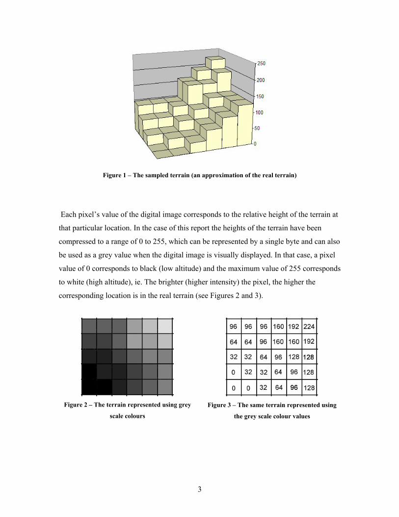
3

Figure 1 – The sampled terrain (an approximation of the real terrain)

Each pixel’s value of the digital image corresponds to the relative height of the terrain at

that particular location. In the case of this report the heights of the terrain have been

compressed to a range of 0 to 255, which can be represented by a single byte and can also

be used as a grey value when the digital image is visually displayed. In that case, a pixel

value of 0 corresponds to black (low altitude) and the maximum value of 255 corresponds

to white (high altitude), ie. The brighter (higher intensity) the pixel, the higher the

corresponding location is in the real terrain (see Figures 2 and 3).

Figure 2 – The terrain represented using grey

scale colours

Figure 3 – The same terrain represented using

the grey scale colour values

4

2.2 Adjacencies:

To find a path from a starting node to a goal node, we must define a way in which

successor nodes can be selected, ie. Where can we move to from a given location? In the

real world, a person can take a step in any direction he/she pleases but on our digital

terrain maps we are more restricted in our choices. There are two common approaches; 4-

adjacency (see Figure 3) and 8-adjacency (see Figure 4). 4-adjacency restricts the

movement to the four main wind directions: north, south, west and east. 8-adjacency

allows more freedom in movement as it, in addition to the directions of 4-adjacency, also

allows movement in the northeast, northwest, southwest and southeast directions.

Figure 3 – 4-adjacency

Figure 4 – 8-adjacency

Figure 5– 16-adjacency

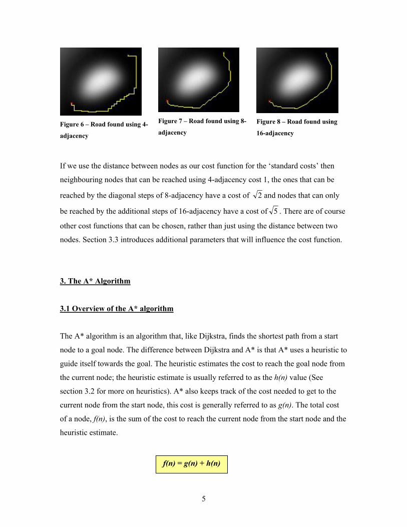
In addition to 4 and 8 adjacency, we can also use 16-adjacency (see Figure 5) which

allows even greater freedom of movement as we can now move north-north-east, north-

east-east, etc. Using 16-adjacency, we can also achieve a smoother looking road by

reducing the sharpness of the turns (see Figures 6, 7 and 8 for comparison). To reduce

sharp turns even further we can penalize sharp turns, for example, it is cheaper to turn 45

degrees rather than 90 degrees. See section 3.3.2 for more detail.

5

Figure 6 – Road found using 4-

adjacency

Figure 7 – Road found using 8-

adjacency

Figure 8 – Road found using

16-adjacency

If we use the distance between nodes as our cost function for the ‘standard costs’ then

neighbouring nodes that can be reached using 4-adjacency cost 1, the ones that can be

reached by the diagonal steps of 8-adjacency have a cost of 2 and nodes that can only

be reached by the additional steps of 16-adjacency have a cost of 5 . There are of course

other cost functions that can be chosen, rather than just using the distance between two

nodes. Section 3.3 introduces additional parameters that will influence the cost function.

3. The A* Algorithm

3.1 Overview of the A* algorithm

The A* algorithm is an algorithm that, like Dijkstra, finds the shortest path from a start

node to a goal node. The difference between Dijkstra and A* is that A* uses a heuristic to

guide itself towards the goal. The heuristic estimates the cost to reach the goal node from

the current node; the heuristic estimate is usually referred to as the h(n) value (See

section 3.2 for more on heuristics). A* also keeps track of the cost needed to get to the

current node from the start node, this cost is generally referred to as g(n). The total cost

of a node, f(n), is the sum of the cost to reach the current node from the start node and the

heuristic estimate.

f(n) = g(n) + h(n)

6

An integral part of the A* algorithm are the open and closed lists. The open list contains

all the nodes that have been reached but haven’t been visited and expanded yet. The

closed list contains all the nodes that have been visited and expanded, ie. They have been

removed from the open list and added to the closed list. A* moves to a successor node by

choosing the most promising node (the one with the lowest f(n) value) from it’s list of

potential successor nodes (ie. from the open list).

A* algorithm pseudocode:

Setup the start node Setup the goal node Create an empty open list Create an empty closed list Add start node to open list while( open list is not empty) {

Pick the node with the lowest f(n) value from the open list and make it the current node if (current node matches goal node) return the current node.

Find all successor nodes from the current node For each successor node { Set it’s g(n) value to the g(n) value of the current node plus the cost to get from the current node to this successor node find the successor node on the open list if(successor node is on open list && existing one has a lower g(n) value) continue if(successor node is on closed list && existing one has a lower g(n) value) continue Remove occurrences of this successor node from the open and closed lists Set the parent of the successor node to the current node Use the heuristic to estimate the distance to the goal node, ie. h(n) Add this successor node to the open list } Add current node to the closed list }

7

3.2 Heuristics

As we have mentioned already, the heuristic part (the h(n) component) used by the A*

algorithm is what differentiates it from Dijkstra’s algorithm by guiding the search

towards the goal node. If the heuristic function is admissible (meaning it never

overestimates the minimum cost to the goal), then A* is also, like Dijkstra, guaranteed to

find the shortest/cheapest path. It is also of great advantage to use a heuristic that

underestimates the minimum cost as little as possible, as this will result in fewer nodes to

be examined (see section 5.3 for a comparison of heuristics). An ideal heuristic will

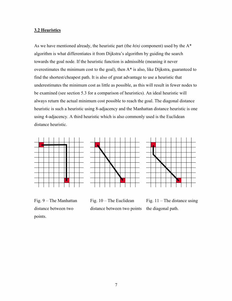
always return the actual minimum cost possible to reach the goal. The diagonal distance

heuristic is such a heuristic using 8-adjacency and the Manhattan distance heuristic is one

using 4-adjacency. A third heuristic which is also commonly used is the Euclidean

distance heuristic.

Fig. 9 – The Manhattan

distance between two

points.

Fig. 10 – The Euclidean

distance between two points

Fig. 11 – The distance using

the diagonal path.

8

a) Manhattan distance heuristic (Fig. 9)

The Manhattan heuristic is computed by adding together the differences in the x

and y components. The advantage of using this heuristic is that it is

computationally inexpensive.

||||)( baba yyxxnh −+−=

The major drawback of the Manhattan heuristic is the fact that it tends to

overestimate the actual minimum cost to the goal (unless 4-adjacency is used)

which means that the road being found may not be an optimal solution. If we are

not interested in an optimal solution, just a good one, then using an

overestimating heuristic can speed up the road finding (see section 5.3).

b) Euclidean distance heuristic (Fig. 10)

The Euclidean heuristic is admissible, but usually underestimates the actual cost

by a significant amount. This means that we may visit too many nodes

unnecessarily which in turn increases the time it takes to find the road. The

Euclidean distance heuristic is also computationally more expensive to apply

compared to the Manhattan heuristic, as it additionally involves two

multiplication operations and taking the square root.

2 22 )()()( baba yyxxnh −+−=

c) Diagonal distance heuristic (Fig. 11)

The diagonal distance heuristic combines aspects of both the Manhattan and

Euclidean heuristics. The resultant heuristic is admissible (unless 16-adjacency is

9

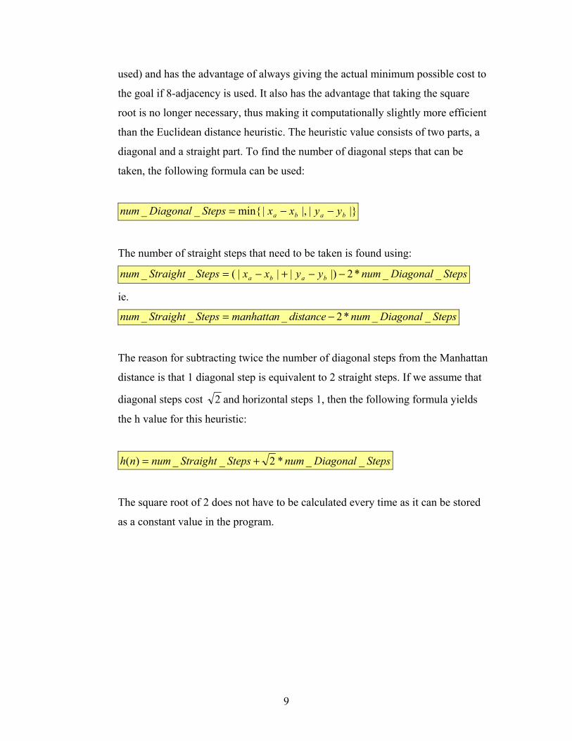
used) and has the advantage of always giving the actual minimum possible cost to

the goal if 8-adjacency is used. It also has the advantage that taking the square

root is no longer necessary, thus making it computationally slightly more efficient

than the Euclidean distance heuristic. The heuristic value consists of two parts, a

diagonal and a straight part. To find the number of diagonal steps that can be

taken, the following formula can be used:

|}||,|min{__ baba yyxxStepsDiagonalnum −−=

The number of straight steps that need to be taken is found using:

StepsDiagonalnumyyxxStepsStraightnum baba __*2|)|||(__ −−+−=

ie.

StepsDiagonalnumancetdisnmanhattaStepsStraightnum __*2___ −=

The reason for subtracting twice the number of diagonal steps from the Manhattan

distance is that 1 diagonal step is equivalent to 2 straight steps. If we assume that

diagonal steps cost 2 and horizontal steps 1, then the following formula yields

the h value for this heuristic:

StepsDiagonalnumStepsStraightnumnh __*2__)( +=

The square root of 2 does not have to be calculated every time as it can be stored

as a constant value in the program.

10

3.3 User defined constraints

3.3.1 Gradients and Gradient Penalties

The reason for introducing gradient penalties is that realistic roads generally have a

maximum gradient. The Cornwall County Council, for instance, limits the maximum

gradient for traditional surfaced roads to 10%, ie 1 in 10 [8]. There are many reasons for

imposing a maximum gradient, for example:

• Safety Reasons – vehicles traveling downhill have greater stopping distances.

• Vehicle Considerations – Some vehicles, especially heavy loaded trucks, would

have great difficulties traveling uphill.

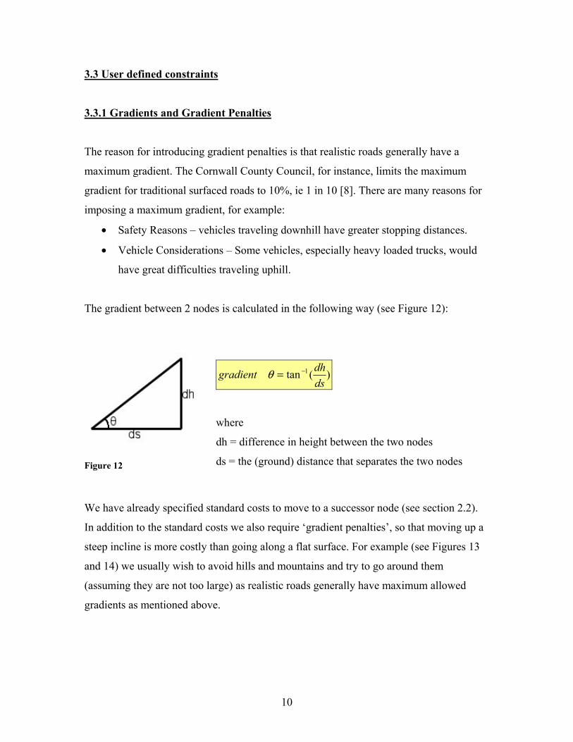
The gradient between 2 nodes is calculated in the following way (see Figure 12):

Figure 12

)(tan 1

dsdhgradient −=θ

where

dh = difference in height between the two nodes

ds = the (ground) distance that separates the two nodes

We have already specified standard costs to move to a successor node (see section 2.2).

In addition to the standard costs we also require ‘gradient penalties’, so that moving up a

steep incline is more costly than going along a flat surface. For example (see Figures 13

and 14) we usually wish to avoid hills and mountains and try to go around them

(assuming they are not too large) as realistic roads generally have maximum allowed

gradients as mentioned above.

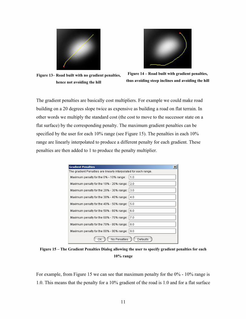
11

Figure 13– Road built with no gradient penalties,

hence not avoiding the hill

Figure 14 – Road built with gradient penalties,

thus avoiding steep inclines and avoiding the hill

The gradient penalties are basically cost multipliers. For example we could make road

building on a 20 degrees slope twice as expensive as building a road on flat terrain. In

other words we multiply the standard cost (the cost to move to the successor state on a

flat surface) by the corresponding penalty. The maximum gradient penalties can be

specified by the user for each 10% range (see Figure 15). The penalties in each 10%

range are linearly interpolated to produce a different penalty for each gradient. These

penalties are then added to 1 to produce the penalty multiplier.

Figure 15 – The Gradient Penalties Dialog allowing the user to specify gradient penalties for each

10% range

For example, from Figure 15 we can see that maximum penalty for the 0% - 10% range is

1.0. This means that the penalty for a 10% gradient of the road is 1.0 and for a flat surface

12

with a gradient of 0% is 0. All the values between 0% and 10% are linearly interpolated.

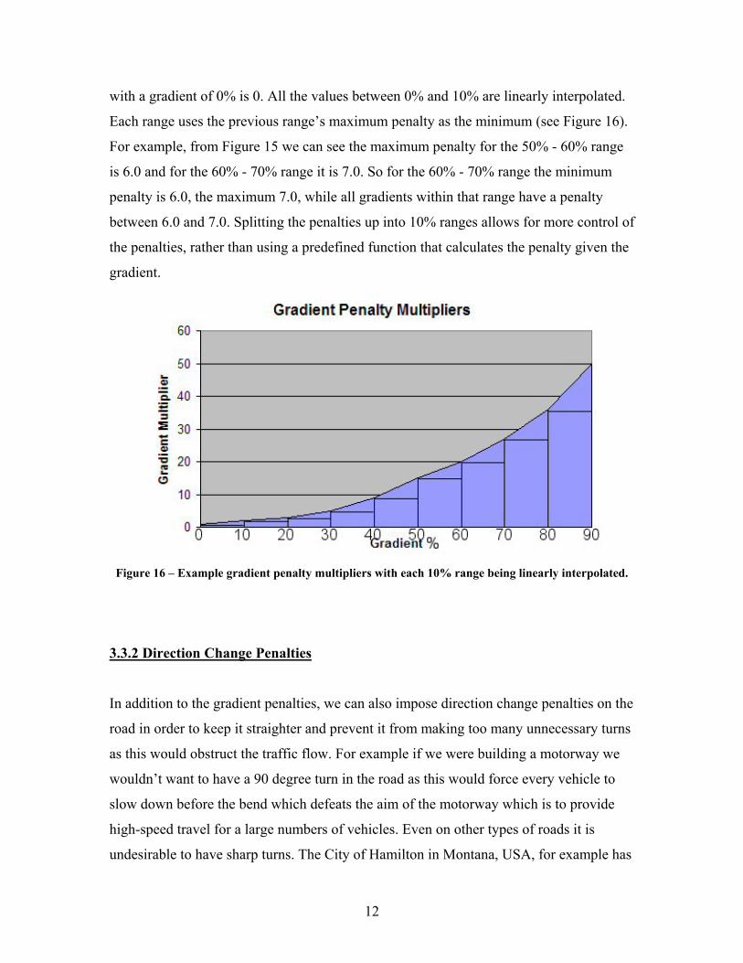
Each range uses the previous range’s maximum penalty as the minimum (see Figure 16).

For example, from Figure 15 we can see the maximum penalty for the 50% - 60% range

is 6.0 and for the 60% - 70% range it is 7.0. So for the 60% - 70% range the minimum

penalty is 6.0, the maximum 7.0, while all gradients within that range have a penalty

between 6.0 and 7.0. Splitting the penalties up into 10% ranges allows for more control of

the penalties, rather than using a predefined function that calculates the penalty given the

gradient.

Figure 16 – Example gradient penalty multipliers with each 10% range being linearly interpolated.

3.3.2 Direction Change Penalties

In addition to the gradient penalties, we can also impose direction change penalties on the

road in order to keep it straighter and prevent it from making too many unnecessary turns

as this would obstruct the traffic flow. For example if we were building a motorway we

wouldn’t want to have a 90 degree turn in the road as this would force every vehicle to

slow down before the bend which defeats the aim of the motorway which is to provide

high-speed travel for a large numbers of vehicles. Even on other types of roads it is

undesirable to have sharp turns. The City of Hamilton in Montana, USA, for example has

13

a regulation that says that a curve must have a minimum radius of 249 feet in order to

provide a design speed of 30mph [9]. The minimum radii of motorway curves must be

even greater to allow for higher design speeds.

As with the gradient penalties, the user has the freedom to specify the penalties (see

Figure 17).

Figure 17 – The Direction Change Penalty Dialog

The dialog box allows the user to specify the penalties for 7 directions, although not all

are used by all adjacencies. For example, if we are using 16-adjacency we can turn by a

maximum of 7 directions to the left or right. The A* algorithm will never perform a 180

degree turn, as long as the cost to get to a neighbouring node is greater than 0. If we were

using 8-adjacency however, we can only turn by a maximum of 3 directions to the left or

right. The direction change penalty will be added to the gradient penalty multiplier and

then the total cost to the neighbouring node will be calculated, ie.

Total Cost = standard cost * (gradient penalty + direction change penalty)

Where the standard cost is the cost to visit a particular successor assuming no penalties,

ie. Height differences and direction changes have no effect.

14

For example, if the standard cost to a neighbouring node is 1, the gradient penalty is 2.5

and the direction change penalty is 1.5 then the total cost to get to the neighbouring node

is 1*(2.5 + 1.5) = 4.

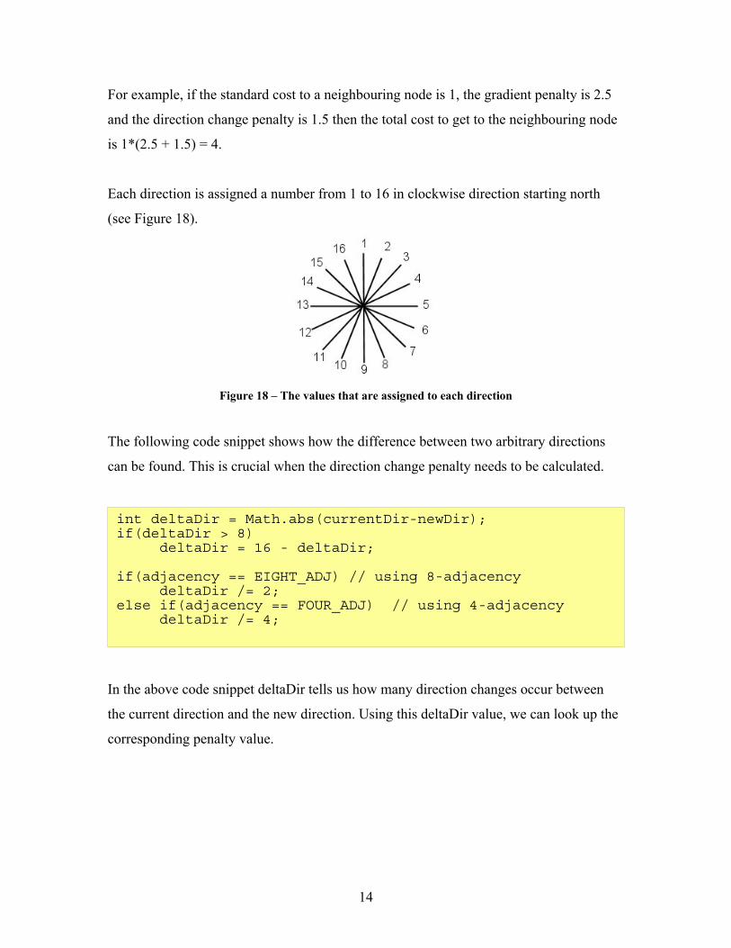
Each direction is assigned a number from 1 to 16 in clockwise direction starting north

(see Figure 18).

Figure 18 – The values that are assigned to each direction

The following code snippet shows how the difference between two arbitrary directions

can be found. This is crucial when the direction change penalty needs to be calculated.

In the above code snippet deltaDir tells us how many direction changes occur between

the current direction and the new direction. Using this deltaDir value, we can look up the

corresponding penalty value.

int deltaDir = Math.abs(currentDir-newDir); if(deltaDir > 8)

deltaDir = 16 - deltaDir;

if(adjacency == EIGHT_ADJ) // using 8-adjacency deltaDir /= 2; else if(adjacency == FOUR_ADJ) // using 4-adjacency deltaDir /= 4;

15

3.4 Variations of the A* algorithm

As we have seen in section 3.1, the open and closed lists are critical aspects of the A*

algorithm. The open list contains all the nodes that are possible candidates for the next

node to be visited and the closed list contains the nodes that have already been visited.

A* will always select the cheapest node from the open list and visit it next. During the

search, especially on large terrains, this list of open nodes (and closed nodes) can grow

very large. This is something we want to avoid, because the larger the list the more

memory is required to store it and the more time is consumed when new nodes are added

to the list, a check is performed whether a node is present in the list or when searching

the list for the node with the smallest f(n) value. The extra time consumption varies with

the data structures used to store the list(s). There are variations of the A* algorithm that

try to improve on the memory and time requirements. However, a reduction in the size of

the search space is usually more effective in minimizing memory and time usage (see

section 4 for terrain sub-sampling).

The Beam Search variation of the A* algorithm imposes a limit on the size of the open

list. The size limit on the open list is referred to as the “beam width”. By imposing a limit

on the open list, the memory requirements of the search are reduced and operations (see

previous paragraph) on the open list occur quicker. Once the limit has been reached the

node with the highest f(n) value (highest cost) is dropped from the open list (and added to

the closed list) to make room for a new node. Depending on the data structure used, it

might be an advantage to delete several nodes (the ones with the highest f(n) values) once

a limit has been reached instead of removing a single node at a time. The major

shortcoming of Beam Search is that it is not optimal and not complete, meaning it may

not necessarily find the shortest path (or any other path) from the start node to the goal

node. This can happen when the node that would have led to the shortest path is

discarded from the open list. Just like A*, the closed list can still grow very large and can

lead to the same memory and time issues mentioned above.

16

Iterative Deepening A* [10] performs a series of searches, where each search has a

maximum cut-off value, ie. a limit on the f(n) value. The cut-off value is increased with

each iteration. The iterations continue until the goal node has been reached or the search

space has been exhausted. Initially the cut-off value should be the h(n) value of the start

node. The question arises by how much we should increase the cut-off value with each

iteration. If we increase it by a small amount, there is the possibility of going through

many iterations; this is a problem if the path is long and each iteration takes a significant

amount of time. If we increase it by a large amount with each iteration, we may visit

many nodes unnecessarily. Just like the standard A* algorithm, iterative deepening A* is

also optimal, ie. it will also return the shortest path.

Searching in one direction (unidirectional search) involves searching a single search tree,

but there is another approach, bidirectional search, that searches two smaller trees

instead. One search starts from the start node searching forwards to the goal node, the

other searching backwards from the goal node to the start node. Because the trees grow

exponentially, the search space created by two small search trees is generally less than

the size of a single large tree assuming that the bidirectional search meets in the middle,

ie. the two smaller search trees are approximately of the same size. Pohl [11, 12] noted

that if there is more than one path from the start node to the goal node, then the two

search fronts seldom meet in the middle. This means that the size of the two ‘smaller’

search trees often exceeds the size of the single search tree created by using a

unidirectional search.

A variation of the bidirectional search is the retargeting approach, first suggested by Pohl

and Politowsky [13]. The retargeting bidirectional search does not perform the forward

and backward searches ‘simultaneously’, but switches between, ie. the forward search is

allowed to run for a certain amount of time, then the backward search, then the forward

search again and so on until a path has been found. In addition to this, instead of aiming

the search towards the goal node and start node, for the forward search and backward

search respectively, each search front aims at the most promising candidate (called the d-

node [13]) of the other search front. Experimental results (see section 5.2) however

17

resulted in poor solutions. The quality of the solution generally improves the longer each

search is allowed to run for.

Another variation of the bidirectional search, suggested by De Champeaux, is the front-

to-front variation [14]. The motivation behind it is to avoid that the two smaller search

trees do not meet in the middle, as discussed above. Unlike the Pohl’s bidirectional

search [11] the two search fronts aim at each other as opposed to aiming at the start or

goal node. Since we are aiming at a search front consisting of several nodes rather than a

single node, it makes the heuristic calculation much more expensive as the heuristic

depends on all the nodes of the opposite search front. In addition to that, new nodes are

continuously expanded thus dynamically changing the search fronts. Politowski and Pohl

[13] showed that even though the two search fronts now meet in the middle reducing the

size of the search space compared to unidirectional search, the extra time needed to

compute the heuristic values tends to exceed the time it would have taken to search the

extra nodes with unidirectional search.

4. Terrain Sub-sampling

4.1 Single Terrain sub-sampling

We previously mentioned that the search space can be very large and thus searching

through it can take a long time and use up a lot of memory and other resources. We have

seen that there are variations of the A* algorithm (see section 3.4), that try to address

some of these problems, but a better approach is to try and decrease the size of the search

space. This can be accomplished by sub-sampling the terrain.

18

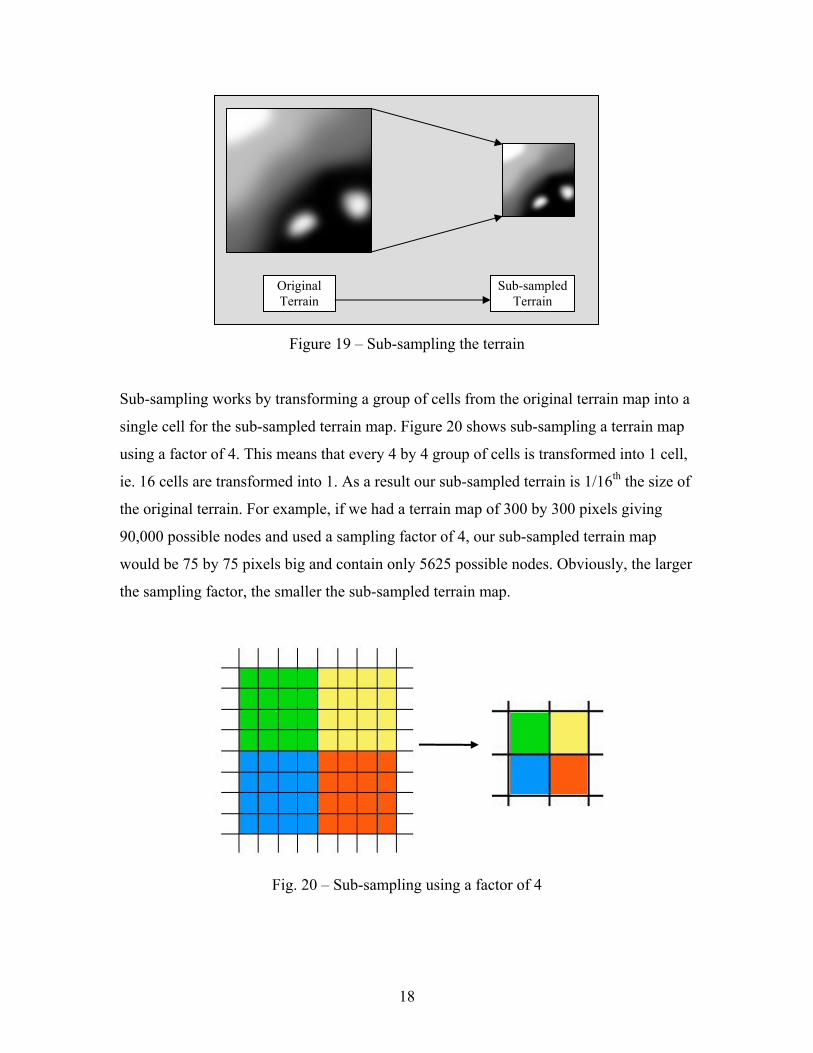
Figure 19 – Sub-sampling the terrain

Sub-sampling works by transforming a group of cells from the original terrain map into a

single cell for the sub-sampled terrain map. Figure 20 shows sub-sampling a terrain map

using a factor of 4. This means that every 4 by 4 group of cells is transformed into 1 cell,

ie. 16 cells are transformed into 1. As a result our sub-sampled terrain is 1/16th the size of

the original terrain. For example, if we had a terrain map of 300 by 300 pixels giving

90,000 possible nodes and used a sampling factor of 4, our sub-sampled terrain map

would be 75 by 75 pixels big and contain only 5625 possible nodes. Obviously, the larger

the sampling factor, the smaller the sub-sampled terrain map.

Fig. 20 – Sub-sampling using a factor of 4

Original Terrain

Sub-sampled Terrain

19

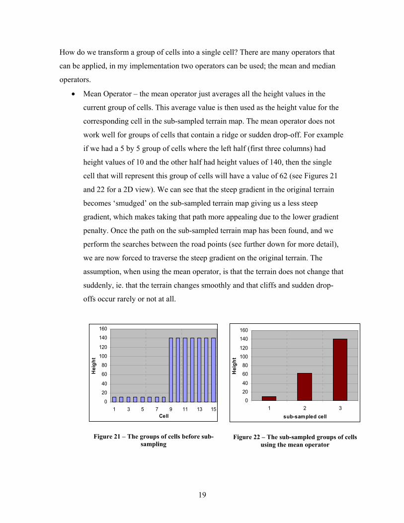
How do we transform a group of cells into a single cell? There are many operators that

can be applied, in my implementation two operators can be used; the mean and median

operators.

• Mean Operator – the mean operator just averages all the height values in the

current group of cells. This average value is then used as the height value for the

corresponding cell in the sub-sampled terrain map. The mean operator does not

work well for groups of cells that contain a ridge or sudden drop-off. For example

if we had a 5 by 5 group of cells where the left half (first three columns) had

height values of 10 and the other half had height values of 140, then the single

cell that will represent this group of cells will have a value of 62 (see Figures 21

and 22 for a 2D view). We can see that the steep gradient in the original terrain

becomes ‘smudged’ on the sub-sampled terrain map giving us a less steep

gradient, which makes taking that path more appealing due to the lower gradient

penalty. Once the path on the sub-sampled terrain map has been found, and we

perform the searches between the road points (see further down for more detail),

we are now forced to traverse the steep gradient on the original terrain. The

assumption, when using the mean operator, is that the terrain does not change that

suddenly, ie. that the terrain changes smoothly and that cliffs and sudden drop-

offs occur rarely or not at all.

0

20

40

60

80

100

120

140

160

1 3 5 7 9 11 13 15Cell

Hei

ght

Figure 21 – The groups of cells before sub-sampling

02040

6080

100120

140160

1 2 3sub-sampled cell

Hei

ght

Figure 22 – The sub-sampled groups of cells using the mean operator

20

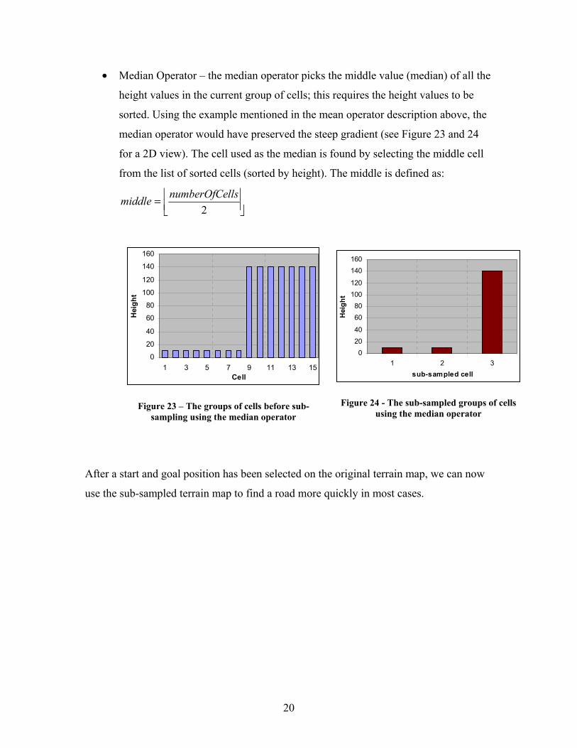
• Median Operator – the median operator picks the middle value (median) of all the

height values in the current group of cells; this requires the height values to be

sorted. Using the example mentioned in the mean operator description above, the

median operator would have preserved the steep gradient (see Figure 23 and 24

for a 2D view). The cell used as the median is found by selecting the middle cell

from the list of sorted cells (sorted by height). The middle is defined as:

⎥⎦⎥

⎢⎣⎢=

2llsnumberOfCemiddle

0

20

40

60

80

100

120

140

160

1 3 5 7 9 11 13 15Cell

Hei

ght

Figure 23 – The groups of cells before sub-sampling using the median operator

02040

6080

100120

140160

1 2 3sub-sampled cell

Hei

ght

Figure 24 - The sub-sampled groups of cells using the median operator

After a start and goal position has been selected on the original terrain map, we can now

use the sub-sampled terrain map to find a road more quickly in most cases.

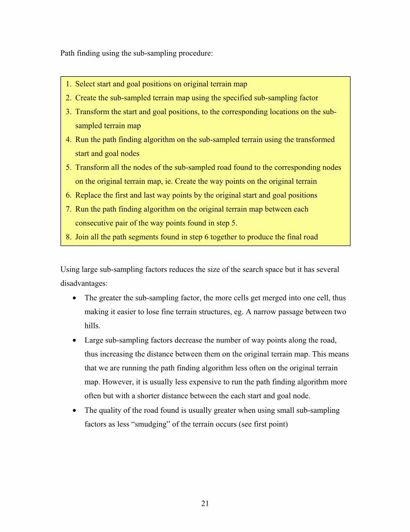
21

Path finding using the sub-sampling procedure:

Using large sub-sampling factors reduces the size of the search space but it has several

disadvantages:

• The greater the sub-sampling factor, the more cells get merged into one cell, thus

making it easier to lose fine terrain structures, eg. A narrow passage between two

hills.

• Large sub-sampling factors decrease the number of way points along the road,

thus increasing the distance between them on the original terrain map. This means

that we are running the path finding algorithm less often on the original terrain

map. However, it is usually less expensive to run the path finding algorithm more

often but with a shorter distance between the each start and goal node.

• The quality of the road found is usually greater when using small sub-sampling

factors as less “smudging” of the terrain occurs (see first point)

1. Select start and goal positions on original terrain map

2. Create the sub-sampled terrain map using the specified sub-sampling factor

3. Transform the start and goal positions, to the corresponding locations on the sub-

sampled terrain map

4. Run the path finding algorithm on the sub-sampled terrain using the transformed

start and goal nodes

5. Transform all the nodes of the sub-sampled road found to the corresponding nodes

on the original terrain map, ie. Create the way points on the original terrain

6. Replace the first and last way points by the original start and goal positions

7. Run the path finding algorithm on the original terrain map between each

consecutive pair of the way points found in step 5.

8. Join all the path segments found in step 6 together to produce the final road

22

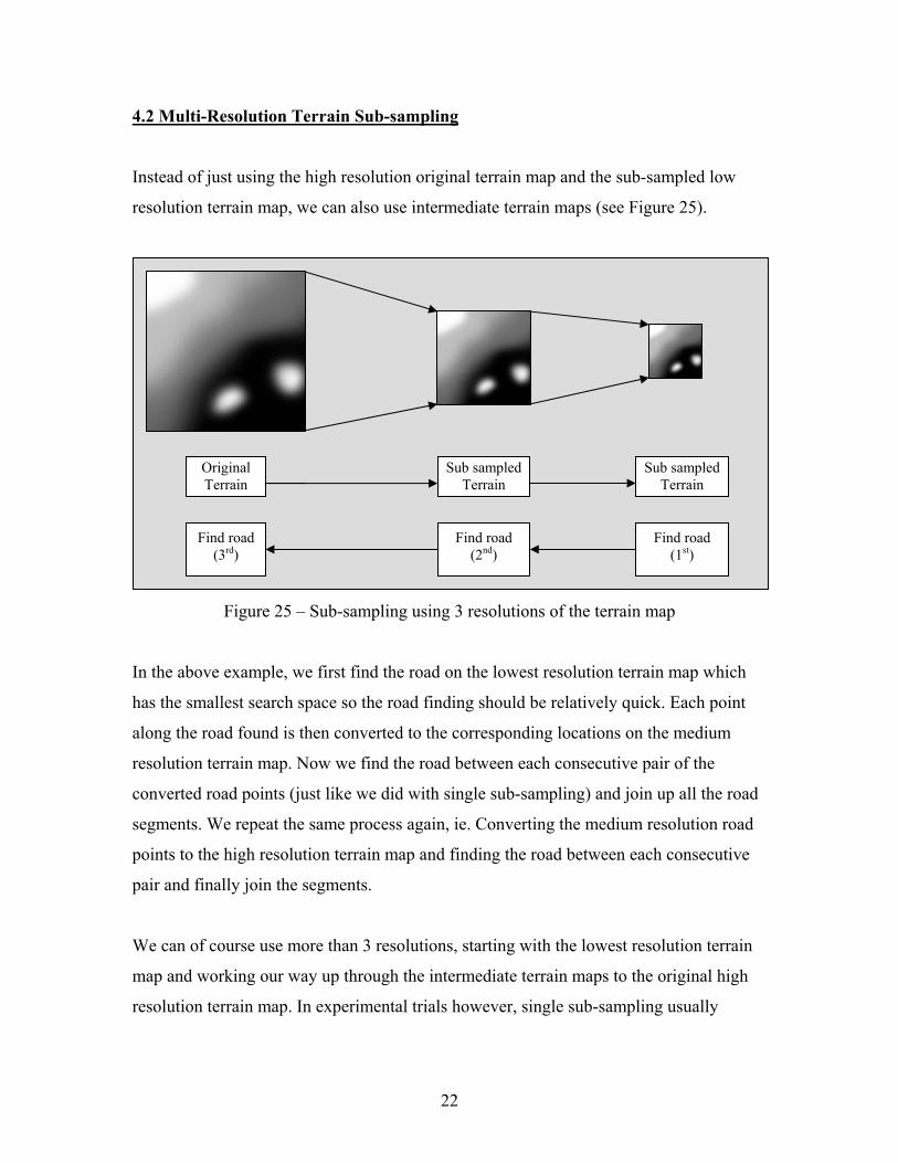
4.2 Multi-Resolution Terrain Sub-sampling

Instead of just using the high resolution original terrain map and the sub-sampled low

resolution terrain map, we can also use intermediate terrain maps (see Figure 25).

Figure 25 – Sub-sampling using 3 resolutions of the terrain map

In the above example, we first find the road on the lowest resolution terrain map which

has the smallest search space so the road finding should be relatively quick. Each point

along the road found is then converted to the corresponding locations on the medium

resolution terrain map. Now we find the road between each consecutive pair of the

converted road points (just like we did with single sub-sampling) and join up all the road

segments. We repeat the same process again, ie. Converting the medium resolution road

points to the high resolution terrain map and finding the road between each consecutive

pair and finally join the segments.

We can of course use more than 3 resolutions, starting with the lowest resolution terrain

map and working our way up through the intermediate terrain maps to the original high

resolution terrain map. In experimental trials however, single sub-sampling usually

Original Terrain

Sub sampled Terrain

Sub sampled Terrain

Find road (1st)

Find road (2nd)

Find road (3rd)

23

results in higher quality roads found than using multi-resolution sub-sampling (see

section 5.4).

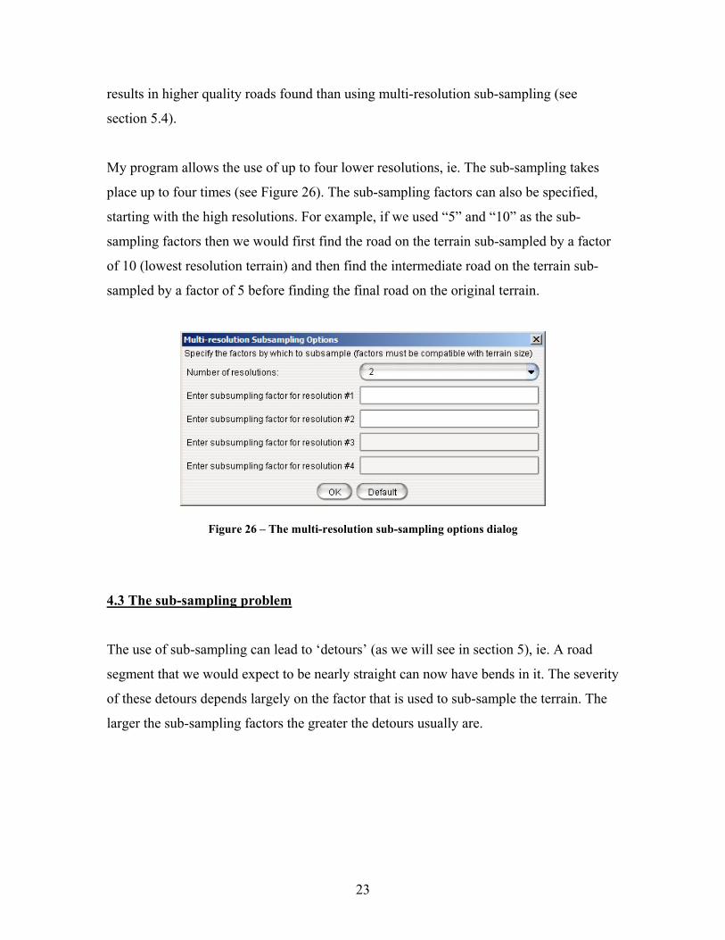
My program allows the use of up to four lower resolutions, ie. The sub-sampling takes

place up to four times (see Figure 26). The sub-sampling factors can also be specified,

starting with the high resolutions. For example, if we used “5” and “10” as the sub-

sampling factors then we would first find the road on the terrain sub-sampled by a factor

of 10 (lowest resolution terrain) and then find the intermediate road on the terrain sub-

sampled by a factor of 5 before finding the final road on the original terrain.

Figure 26 – The multi-resolution sub-sampling options dialog

4.3 The sub-sampling problem

The use of sub-sampling can lead to ‘detours’ (as we will see in section 5), ie. A road

segment that we would expect to be nearly straight can now have bends in it. The severity

of these detours depends largely on the factor that is used to sub-sample the terrain. The

larger the sub-sampling factors the greater the detours usually are.

24

Figure 27 – Sub-sampling problem.

The green line and points show the actual road on the high resolution terrain, but when

sub-sampling comes into place, all the points in one region (see white/grey shading) are

transformed into one point. This point is then used for the road finding for the low

resolution terrain map (see the left side of Figure 27) and once the road has been found,

the points are transformed back to the high resolution terrain map. These transformed

points now lie in the centre of each region. This means that even though the road along

those 2 segments would have been nearly a straight line, using sub-sampling we now

have a 90 degree bend in the road. This produces the detours we can often see on roads

found using sub-sampling. As the sub-sampling factor increases, the detours become

more extreme due to the greater distance between the way points.

5. Experimental Results and Comparisons

5.1 Comparison of different single sub-sampling factors:

Settings: Default gradient penalties, default direction change penalties, 16-adjacency, A*

algorithm, diagonal distance heuristic. The road found with no sub-sampling is included

for comparison.

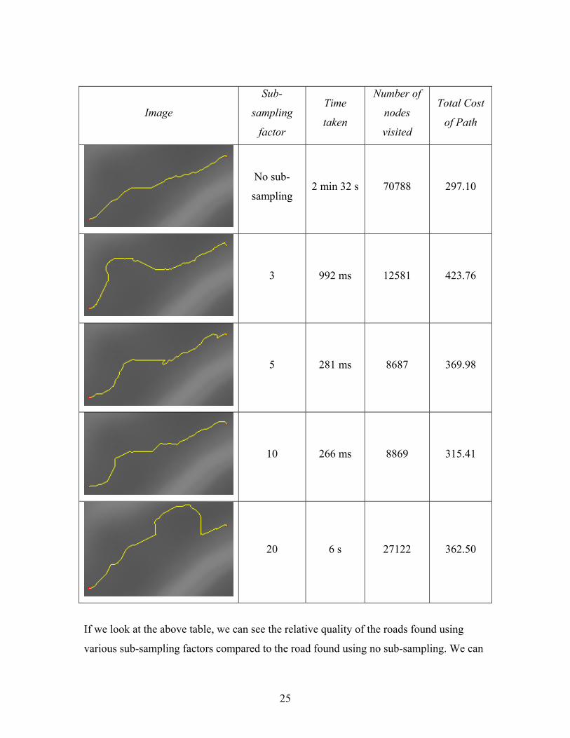
25

Image

Sub-

sampling

factor

Time

taken

Number of

nodes

visited

Total Cost

of Path

No sub-

sampling 2 min 32 s 70788 297.10

3 992 ms 12581 423.76

5 281 ms 8687 369.98

10 266 ms 8869 315.41

20 6 s 27122 362.50

If we look at the above table, we can see the relative quality of the roads found using

various sub-sampling factors compared to the road found using no sub-sampling. We can

26

see that as the sub-sampling factor increases, the smoothness of the road decreases. The

roads found using sub-sampling factors of 5 and 10 produced reasonable roads, while the

quality of the roads found using sub-sampling factors of 3 and 20 produced less satisfying

roads. The road found using a sub-sampling factor of 10 produced the best one compared

to the other sub-sampling factors in this case. Compared to the road found with no sub-

sampling, the road was found in only 266 ms instead of 2 minutes and 32 seconds, a huge

improvement. It also visited only 8869 nodes (~12.5% of the nodes visited without sub-

sampling). The detour that sometimes occurs with rounds found using sub-sampling is

due to the sub-sampling problem discussed in section 4.3. Also interesting to note are the

differences in the running times of the various sub-sampling factors. Using a sub-

sampling factor of 10 proved to be the quickest, closely followed by factor 5, both being

under the 300ms mark. Sub-sampling using factor 3 took nearly a second while sub-

sampling using factor 20 took longest at ~6s. The reason for the factors 5 and 10 being

the quickest is that those sub-sampling factors are near the ‘optimum’ equilibrium sub-

sampling factor. Sub-sampling using factor 3 means that the road on the sub-sampled

terrain contains more way points which lie close together on the high resolution terrain

thus making the search between the way points very fast, ie. We do a lot of small

searches. If we are sub-sampling at a factor of 20 we do the opposite, we do very few

searches on the high resolution terrain since the distance between the way points is

greater (see section 4.1). The other two sub-sampling factors, “5” and “10”, lie in

between; the distance between the way points is moderately large and the searches on the

high resolution terrain occur moderately often.

5.2 Comparison of different algorithms:

Settings: Default gradient penalties, default direction change penalties, diagonal distance

heuristic, 16-adjacency.

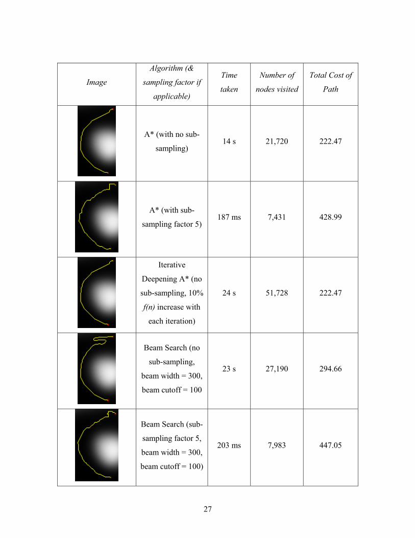
27

Image

Algorithm (&

sampling factor if

applicable)

Time

taken

Number of

nodes visited

Total Cost of

Path

A* (with no sub-

sampling) 14 s 21,720 222.47

A* (with sub-

sampling factor 5) 187 ms 7,431 428.99

Iterative

Deepening A* (no

sub-sampling, 10%

f(n) increase with

each iteration)

24 s 51,728 222.47

Beam Search (no

sub-sampling,

beam width = 300,

beam cutoff = 100

23 s 27,190 294.66

Beam Search (sub-

sampling factor 5,

beam width = 300,

beam cutoff = 100)

203 ms 7,983 447.05

28

Retargeting Search

(no sub-sampling,

each search front

visits 100 nodes at

a time)

218 ms 13,934 470.36

From the above table we can clearly see that the A* algorithm with no sub-sampling

produced the best road, having the smallest total cost. Using the A* algorithm with a sub-

sampling factor of 5 took a fraction of that time (only ~187 ms) and produced a

reasonable road. The iterative deepening approach of the A* algorithm produced the

same road as the normal A* algorithm but due to the additional iterations visited more

than twice as many nodes and took ~10s longer to run. The performance of the iterative

deepening A* algorithm (and the other algorithms) could be improved by refining the

heuristic so that instead of just estimating the cost to the goal based on a flat surface

would take the gradients into account as well. The Beam Search with no sub-sampling

produced an interesting road in this example. The lower part of the road looks almost

identical to the road produced by the A* algorithm but the upper half contains a “S”

shaped curve in the road that has some similarity to real roads leading up a mountain, like

some of the alpine roads in the European Alps (see Figure 28). Using the Beam Search

with sub-sampling resulted in a road that is very similar to the road produced using A*

with sub-sampling. This is due to the fact that we usually reach our current goal before

the width of the beam is exceeded. The retargeting search produced a relatively poor road

having the largest total cost, as expected, since the search fronts alternate often and

always aim at the current best of the other search front. The ‘current best’ node appears to

be the most promising node locally, but would make for a very poor choice globally.

29

Figure 28 - Passo Dello Stelvio, Italy, alpine road in the European Alps

5.3 Comparison of different heuristics:

Settings: Default gradient penalties, default direction change penalties, 16-adjacency, A*

algorithm with no sub-sampling, diagonal distance heuristic.

Image Heuristic Time taken Number of

nodes visited

Total Cost of

Path

Manhattan

Distance 10 s 19488 300.64

Euclidean

Distance 18 s 24057 300.54

Diagonal

Distance 17 s 23135 300.54

30

From the table above we can see that paths found using the different heuristics are

virtually the same. In fact, the roads found using the Euclidean and diagonal distance

heuristics are exactly the same while the road found using the Manhattan heuristic is only

marginally worse. Since we are using 16-adjacency, the only heuristic that is admissible

is the Euclidean distance, that is, it is the only one that never overestimates the minimum

cost to get to the goal node and thus is guaranteed to find the shortest road. Both the

Manhattan distance and diagonal distance heuristics tend to overestimate the minimum

distance to the goal node, with the Manhattan distance heuristic usually overestimating

by a much larger amount compared to the diagonal distance heuristic. Using an

inadmissible heuristic means that we may not get an optimal solution but it has the

advantage that the search visits fewer nodes and thus takes a shorter time to run. This can

be observed from the above table; the road found using the Manhattan heuristic took only

10 seconds to run while the other heuristics took 7-8 seconds longer. It can also be seen

that the search guided by the Manhattan heuristic visited approximately 4,500 fewer

nodes than the search using the Euclidean distance heuristic and approximately 3,500

fewer nodes than the search guided by the diagonal distance heuristic.

5.4 Comparison of different sub-sampling techniques:

Settings: Default gradient penalties, default direction change penalties, 16-adjacency,

diagonal distance heuristic.

31

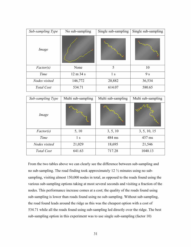
Sub-sampling Type No sub-sampling Single sub-sampling Single sub-sampling

Image

Factor(s) None 5 10

Time 12 m 34 s 1 s 9 s

Nodes visited 146,772 20,882 36,534

Total Cost 534.71 614.07 580.65

Sub-sampling Type Multi sub-sampling Multi sub-sampling Multi sub-sampling

Image

Factor(s) 5, 10 3, 5, 10 3, 5, 10, 15

Time 1 s 484 ms 437 ms

Nodes visited 21,029 18,695 21,546

Total Cost 641.63 717.28 1040.13

From the two tables above we can clearly see the difference between sub-sampling and

no sub-sampling. The road finding took approximately 12 ½ minutes using no sub-

sampling, visiting almost 150,000 nodes in total, as opposed to the roads found using the

various sub-sampling options taking at most several seconds and visiting a fraction of the

nodes. This performance increase comes at a cost; the quality of the roads found using

sub-sampling is lower than roads found using no sub-sampling. Without sub-sampling,

the road found leads around the ridge as this was the cheapest option with a cost of

534.71 while all the roads found using sub-sampling led directly over the ridge. The best

sub-sampling option in this experiment was to use single sub-sampling (factor 10)

32

resulting in a reasonable road with a cost of 580.65. This road is slightly more expensive

than the optimal road (approximately 8.6% more expensive), but the road was found in

only 9 seconds. The roads using multi-resolution sub-sampling were found even faster,

but resulted in worse roads. The more intermediate resolutions we use the faster the roads

are found but also the worse the quality of the roads get. We must realize however that if

we use too many resolutions, then we may spend more time on sub-sampling the terrains

than on the actual searching. We can see from the above table that the road found using 4

additional resolutions resulted in a poor path that is almost twice as expensive as the

optimal road. The more resolutions we use, the larger the sub-sampling factors get which

result in the detours caused by the sub-sampling problem described in section 4.3.

5.5 Comparison of different gradient penalty functions:

Settings: Default direction change penalties, 16-adjacency, diagonal distance heuristic,

A* algorithm.

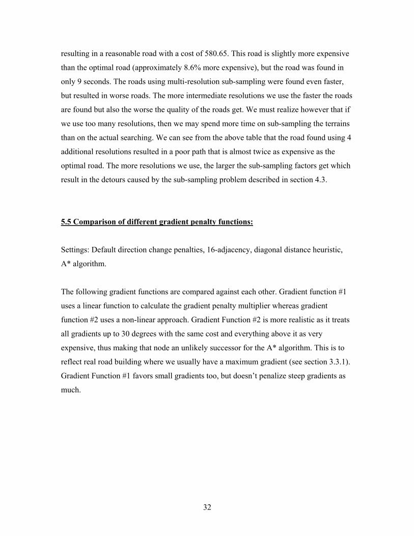
The following gradient functions are compared against each other. Gradient function #1

uses a linear function to calculate the gradient penalty multiplier whereas gradient

function #2 uses a non-linear approach. Gradient Function #2 is more realistic as it treats

all gradients up to 30 degrees with the same cost and everything above it as very

expensive, thus making that node an unlikely successor for the A* algorithm. This is to

reflect real road building where we usually have a maximum gradient (see section 3.3.1).

Gradient Function #1 favors small gradients too, but doesn’t penalize steep gradients as

much.

33

Gradient Function #1

Gradient Function #1

02468

10

0 10 20 30 40 50 60 70 80 90 100

Gradient (degrees)

Gra

dien

t Pen

alty

M

ultip

lier

Gradient Function #2

Gradient Function #2

05

10152025

0 10 20 30 40 50 60 70 80 90 100

Gradient (degrees)

Gra

dien

t Pen

alty

M

ultip

lier

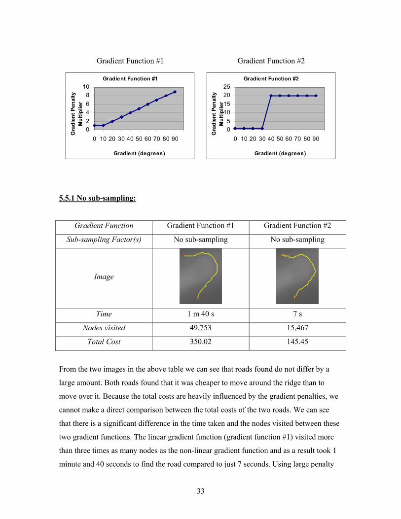
5.5.1 No sub-sampling:

Gradient Function Gradient Function #1 Gradient Function #2

Sub-sampling Factor(s) No sub-sampling No sub-sampling

Image

Time 1 m 40 s 7 s

Nodes visited 49,753 15,467

Total Cost 350.02 145.45

From the two images in the above table we can see that roads found do not differ by a

large amount. Both roads found that it was cheaper to move around the ridge than to

move over it. Because the total costs are heavily influenced by the gradient penalties, we

cannot make a direct comparison between the total costs of the two roads. We can see

that there is a significant difference in the time taken and the nodes visited between these

two gradient functions. The linear gradient function (gradient function #1) visited more

than three times as many nodes as the non-linear gradient function and as a result took 1

minute and 40 seconds to find the road compared to just 7 seconds. Using large penalty

34

multipliers for gradients above a certain threshold can reduce the size of the search space

since it is now very expensive to visit a node that requires the traversal of a road with a

large gradient. This makes the node unlikely to be visited.

5.5.2 Single sub-sampling:

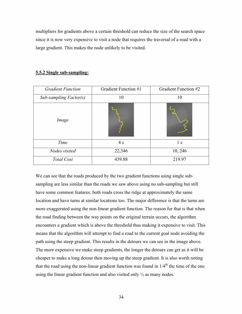
Gradient Function Gradient Function #1 Gradient Function #2

Sub-sampling Factor(s) 10 10

Image

Time 4 s 1 s

Nodes visited 22,346 10, 246

Total Cost 439.88 219.97

We can see that the roads produced by the two gradient functions using single sub-

sampling are less similar than the roads we saw above using no sub-sampling but still

have some common features: both roads cross the ridge at approximately the same

location and have turns at similar locations too. The major difference is that the turns are

more exaggerated using the non-linear gradient function. The reason for that is that when

the road finding between the way points on the original terrain occurs, the algorithm

encounters a gradient which is above the threshold thus making it expensive to visit. This

means that the algorithm will attempt to find a road to the current goal node avoiding the

path using the steep gradient. This results in the detours we can see in the image above.

The more expensive we make steep gradients, the longer the detours can get as it will be

cheaper to make a long detour then moving up the steep gradient. It is also worth noting

that the road using the non-linear gradient function was found in 1/4th the time of the one

using the linear gradient function and also visited only ½ as many nodes.

35

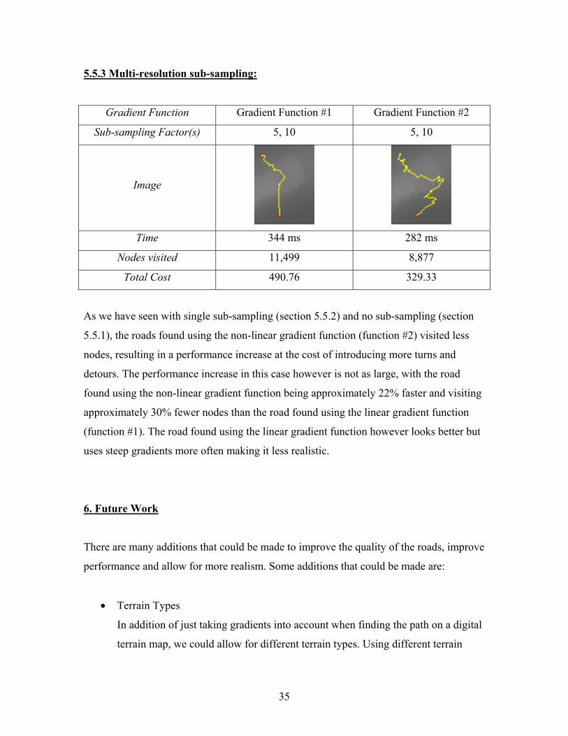
5.5.3 Multi-resolution sub-sampling:

Gradient Function Gradient Function #1 Gradient Function #2

Sub-sampling Factor(s) 5, 10 5, 10

Image

Time 344 ms 282 ms

Nodes visited 11,499 8,877

Total Cost 490.76 329.33

As we have seen with single sub-sampling (section 5.5.2) and no sub-sampling (section

5.5.1), the roads found using the non-linear gradient function (function #2) visited less

nodes, resulting in a performance increase at the cost of introducing more turns and

detours. The performance increase in this case however is not as large, with the road

found using the non-linear gradient function being approximately 22% faster and visiting

approximately 30% fewer nodes than the road found using the linear gradient function

(function #1). The road found using the linear gradient function however looks better but

uses steep gradients more often making it less realistic.

6. Future Work

There are many additions that could be made to improve the quality of the roads, improve

performance and allow for more realism. Some additions that could be made are:

• Terrain Types

In addition of just taking gradients into account when finding the path on a digital

terrain map, we could allow for different terrain types. Using different terrain

36

types we could for example differentiate between water (lakes, rivers etc.) and

earth which would affect the road finding process. Water crossings could be made

more expensive, so that, just like in the real world, we would build a road around

a lake and not build a bridge across it. It could also be useful to define swamp,

forest terrain types etc. as these would also affect the road finding process. It may

not be economically or environmentally feasible to build a road through a dense

forest or swamp. F. Markus Jönsson [1] used different terrain types for his path

finding paper where vehicles (in particular tanks and defense force vehicles)

move from one location to another while following existing roads if possible and

avoiding enemy units.

• Unrestricted Movement

To improve realism and to achieve smoother looking roads we could allow

movement in any arbitrary direction, not just the predefined directions used by the

4-, 8- or 16-adjacencies used in this report. Since we are using a digital terrain

map, which has discrete data, several questions arise. For example how do we

calculate the height at any arbitrary point and the gradients in any direction?

• Smoothing with Bezier curves

To achieve even smoother looking curves and to reduce the ‘aliasing effect’ that

occurs during sub-sampling we could use Bezier curves. This process would take

place after the road has been found.

• Heuristics in 3 dimensions

If we are using gradient penalties (ie. we are making the road building more

expensive on non-flat terrain) then the heuristics tend to underestimate the

minimum cost to reach the goal more than if we were using no gradient penalties.

This is because the heuristic functions do not include the height differences in the

calculations. As mentioned previously, the more the heuristic underestimates the

more nodes are being visited which as a result increases the running time and

memory requirements. Improving the heuristics so that they estimate the

37

minimum cost to the goal node taking the height differences and gradient

penalties into account as well would reduce the amount of underestimating taking

place. As a result fewer nodes would get visited, thus potentially speeding up the

search and reducing memory usage.

7. Conclusion

We have seen that finding a road between two points on a digital terrain map, which is an

approximation of a real terrain, can take a considerable amount of time and memory

using the standard A* algorithm. We have defined additional constraints which affect the

cost function in order to increase the realism of the roads. An example are the gradient

penalties which can be used to favor roads with low gradients just like real road building

where we often have a maximum allowed gradient. We have introduced variations of the

A* algorithm in order to address the time and memory issues, in particular the Beam

Search variation which imposes a maximum size on the open list which as a result

reduces the amount of memory required to store the open list and also makes operations

on the open list faster. The Beam search variation does not find an optimal solution as it

sometimes removes a node which is currently the least promising node to reach the goal

but would have been the node along the shortest road. It is also not complete so that it

may not find a road at all. The only variation that significantly reduced the running time

of the road finding was the retargeting approach but the roads produced by it were

generally of very poor quality. A more drastic improvement on running times and

memory requirements was obtained by sub-sampling the original terrain, resulting in a

large reduction in the size of the search space. The road finding takes place on the sub-

sampled terrain and after the road is found, all the points along the road are transformed

back to the corresponding locations on the original terrain. We then find the road between

each consecutive pair of the road points. We have seen that the roads produced using a

sub-sampling factor of 5 and 10 produced the best results taking the quality of the road

and running time into account. Using smaller sub-sampling factors often increases the

quality of the road but also takes longer since the sub-sampled terrain is still relatively

38

large. Using large sub-sampling factors (>10) do not improve the running time since the

distance between 2 way points on the original high resolution terrain is relatively large.

The quality also degrades due to the sub-sampling problem discussed in section 4.3. We

have also introduced multi-resolution sub-sampling which uses intermediate resolutions

between the high and low resolutions. The motivation behind multi-resolution sub-

sampling is that we can increase the performance when using large sub-sampling factors

so that the distances between the way points is reduced by using an intermediate

resolution before going back to the high resolution terrain. Multi-resolution sub-sampling

also suffers from the sub-sampling problem (see section 4.3) which can now occur for

every sub-sampled resolution used. The performance gain from using multi-resolution

sub-sampling over single sub-sampling is usually not very significant but the loss in the

quality of the road is significant. Thus the use of multi-resolution sub-sampling is only

appropriate on large high resolution terrains.

39

Bibliography

[1] F. Markus Jönsson, “An optimal pathfinder for vehicles in real-world digital

terrain maps”, 1997

http://www.student.nada.kth.se/~f93-maj/pathfinder/

[2] E. W. Dijkstra, “A note on two problems in connection with graphs”, Numerische

Mathematik, 1959, 1, 269-271

[3] Russell, Peter Norvig, 1995, “Artificial Intelligence – A modern approach”, Best

First Search, 94-97

[4] Stuart Russell, Peter Norvig, 1995, “Artificial Intelligence – A modern

approach”, 97–101

[5] Hart, P.; N.Nilson and B.Raphael. 1968, "A Formal Basis for the

Heuristic Determination of Minimum Cost Paths." IEEE

Transactions on Systems Science and Cybernetics 4, no. 2 (July):

100-107

[6] Inside Scoop – simcity.com, “Programmer's Diary: Traffic Simulation”, by Alex

Peck, http://simcity.ea.com/about/inside_scoop/traffic.php, 2003

[7] “Amit's Thoughts on Path-Finding and A-Star”, Introduction,

http://theory.stanford.edu/~amitp/GameProgramming/AStarComparison.html#S2

[8] Cornwall County Council, “Vertical Design”,

http://www.cornwall.gov.uk/environment/design/section5/des53.htm, Feb 2004

[9] City of Hamilton, Section 16.32.090 Streets and roads,

http://www.cityofhamilton.net/codes/Title_16/32/090.html, 1999

40

[10] Korf, Richard E. 1985, “Iterative-Deepening A*: An Optimal Admissible Tree

Search”. Proceedings of the International Joint Conference on Artificial

Intelligence, Los Altos, California, 1034-1036. Morgan Kaufmann

[11] I. Pohl, “Bi-directional and heuristic search in path problems”, Technical report,

SLAC Report No. 104, Stanford Linear Accelerator Center, CA, 1969.

[12] I. Pohl, “Bi-directional search”, Machine Intelligence 6 (1971) 127- 140

[13] G. Politowski and I. Pohl, “D-node retargeting in bidirectional heuristic search”,

Proc. AAAI-84, Austin, Texas (1984), 274-277.

[14] D. De Champeaux, “Bidirectional heuristic search again”, ACM 30 (1) (1983)

122-132.

Further information:

[i] AI Guru, “Pathfinding”, http://www.aiguru.com/pathfinding.htm, January 2004

[ii] GameDev.net, “Pathfinding and Searching”,

http://www.gamedev.net/reference/list.asp?categoryid=18#94, January 2004

[iii] “Amit's Thoughts on Path-Finding and A-Star”,

http://theory.stanford.edu/~amitp/GameProgramming/, Last modified: Jan 30

2004

[iv] “Game Programming Gems Vol.1”, published by Jennifer Niles, Charles River

Media Inc., 2000, 255-287

41

[v] Gamasutra, “Smart Moves: Intelligent Pathfinding”

http://www.gamasutra.com/features/19990212/sm_01.htm, February 1999

[vi] Gamasutra, “Toward More Realistic Pathfinding”,

http://www.gamasutra.com/features/20010314/pinter_01.htm, March 2001

42

Appendix

Running Instructions:

Note: The skin that is being used in this program is still in the development stage, so it

has some bugs. Sometimes the components are painted incorrectly. The skin is enabled

by default but can be disabled when the program is started.

To run the program with the skin enabled:

Type “java RoadTool” in the command prompt.

To run the program with the skin disabled:

Type “java RoadTool -skin” in the command prompt.

Once the program has started, a terrain can be loaded by clicking on “File” and then

“Open”. A dialog will appear prompting for the selection of a file. It is considerably

faster to load the terrain if it is stored on the local hard drive rather than a network drive.

Once the terrain has loaded, the selection of the start and end points can be made and the

road finding can begin by clicking on “Search” under the “Search” item in the menu bar.

Note that for long paths with no sub-sampling, the search can take a long time. The

search can be cancelled at any time by clicking on “Cancel Search” under the “Search”

item in the menu bar.

Terrain data information:

The terrain files are height maps stored as raw files; the terrains have a file extension of

‘.raw’. The terrain files are 8-bit grayscale values thus allowing values from 0 to 255 for

each pixel. The values are stored row after row. Since the terrain files are stored as raw

files, and contain no file header, they contain no information on the size of the terrain or

its dimension. This information needs to be recorded externally. All the supplied sample

terrain files have a dimension of 300 by 300 pixels. If a terrain is used with dimensions

different from the default 300 by 300 dimension, then a minor change has to be made in

43

the source code so that the loading of the terrain works for this dimension. How to load

terrains with dimensions other than the default 300 by 300:

1. Open the “HeightMap.java” file

2. Change the variables “width” and “height” to the dimension of the terrain file

to be used.

3. Save the file.

4. Compile the file (eg. “javac HeightMap.java”).

5. Run the program.

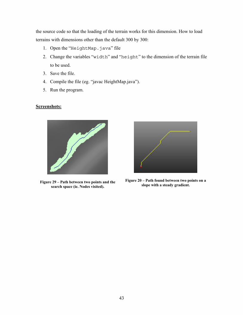
Screenshots:

Figure 29 – Path between two points and the search space (ie. Nodes visited).

Figure 20 – Path found between two points on a slope with a steady gradient.

44

Figure 31 – Path through flat terrain with hills (16 adjacency, A*, no sub-sampling). We can see

the algorithm avoided going up the hills; it is always cheaper to go around them.

Figure 32 - Path through flat terrain with hills (16 adjacency, A*, no sub-sampling). The Search Space is also displayed. We can see that nodes up a hill were never visited as it was always cheaper

to visit nodes along the flat surface.

Figure 33 – The main window of the road tool application with the search menu shown.