automated risk mitigation in business processes...
TRANSCRIPT

Automated Risk Mitigation in Business Processes(extended version)
R. Conforti1, A.H.M. ter Hofstede1,2, M. La Rosa1, and M. Adams1
1 Queensland University of Technology, Australiaraffaele.conforti,a.terhofstede,m.larosa,[email protected]
2 Eindhoven University of Technology, The Netherlands
Abstract. This paper proposes a concrete approach for the automatic mitigationof risks that are detected during process enactment. Given a process model af-fected by risks, e.g. a financial process exposed to the risk of approval fraud, weenact this process and as soon as the likelihood of the associated risk(s) is nolonger tolerable, we generate a set of possible mitigation actions to reduce therisks’ likelihood, ideally annulling the risks altogether. A mitigation action is asequence of controlled changes applied to the running process instance, takinginto account a snapshot of the process resources and data, and the current sta-tus of the system in which the process is executed. These actions are proposedas recommendations to help process administrators mitigate process-related risksas soon as they arise. The approach has been implemented in the YAWL envi-ronment and its performance evaluated. The results show that it is possible tomitigate process-related risks within a few minutes.
1 Introduction
Business processes in various sectors such as financial, healthcare and oil&gas, areconstantly exposed to a wide range of risks. Take for example the BP oil spill in 2010which resulted in an environmental disaster, or the fraud at Societe Generale in 2008,which led to a e 4.9B loss.
A process-related risk measures the likelihood and the consequence that some-thing happening will impact on the process objectives [27]. Failing to address process-related risks can result in substantial financial and reputational consequences, poten-tially threatening an organization’s existence, like in the case of Societe Generale. Thereis thus an increasing need to better manage business process risks, as also highlightedby legislative initiatives like Basel II [8] and the Sarbanes-Oxley Act.3 Organizationsare attempting to incorporate process-related risks as a distinct view in their operationalmanagement, seeking effective ways to control such risks. However, whilst conceptu-ally appealing, to date there is little guidance as to how this can be concretely done.
In previous work [11], we presented a mechanism to model risks in executable busi-ness process models and detect them as early as possible during process execution. Un-fortunately, detecting a risk in time is often not enough to avoid the negative outcomeassociated. A prompt risk mitigation should be taken to restore the process instance to
3 www.gpo.gov/fdsys/pkg/PLAW-107publ204

a safe state, before the instance progresses any further. Moreover, taking the right mit-igation at the right time may make the difference between success and failure. In fact,the number of possible ways a process-related risk may be mitigated is potentially verylarge that is difficult for a process administrator to take the right decision at the righttime, without any support. One has to consider all mitigations that are possible, giventhe current state of the process instance (including a snapshot of the associated dataand resources), and the context in which the instance is running, i.e. the state of otherrunning instances, to make such a decision. For example, in order to mitigate the riskof a process instance A to run overtime, a mitigation may entail to reallocate resourcesfrom a process instance B (potentially of another process) to A.
In light of the above, in this paper we propose a technique for automatically miti-gating process-related risks. Since a process instance may be affected by multiple risksat the same time, we treat this problem as a multi-objective optimization problem. Asolution to this problem is a variant of the risky process instance obtained by apply-ing a sequence of mitigation actions, in order to reduce the risks’ probability down toa tolerable level, or in the best case, to annul the risks altogether. Mitigation actionsinclude control-flow aspects (e.g. skipping a task to be executed), process resources(e.g. reallocating a resource to a different task), and data (e.g. rolling back an executedtask to restore its input data). To explore the potentially large solution space, we usedominance-based Multi-Objective Simulated Annealing (MOSA) [26]. At each run, thealgorithm generates a small set of solutions similar to the original process instance butwith less risks. It stops when either a maximum number of non-redundant solutions (i.e.solutions proposing different mitigations) is found or a given timeframe elapses. Thisapproach is not meant to replace human judgement. Instead, it aims to support processadministrators in deciding what mitigations to take, by reducing the number of feasibleoptions, and consequently the time needed to take a decision.
We defined the mitigation actions in collaboration with an Australian risk consul-tant. To prove the feasibility of this approach, we implemented these actions and theMOSA algorithm on top of the YAWL system. We instantiated a set of process models,inspired by an industry standard [28] and a process model from the area of screen busi-ness [24], affected by one or more risks, and executed a series of tests to mitigate suchrisks. The tests show that the technique can find a set of possible solutions within a fewminutes of computation, and that in all cases the associated risks are mitigated.
The rest of this paper is organized as follows. Section 2 introduces the requiredbackground concepts in the context of an example. Section 3 describes the proposedtechnique to mitigate process risks which is then evaluated in Section 4. Section 5 cov-ers related work and Section 6 concludes the paper. Appendix A describes the processmodels used in the experiments; Appendix B provides the definition of the risks as-sociated with these process models; Appendix C provides the solutions to one of theexperiments in this paper.
2 Background and running exampleOur technique for risk mitigation is part of a holistic approach for managing process-related risks throughout the process lifecycle. Accordingly, the four phases of the tradi-tional BPM lifecycle (Design, Implementation, Enactment and Analysis) [13] are each

extended to incorporate elements of risk, as shown in Fig. 1. First, in a Risk Identifica-tion phase, the process model to be designed is analyzed for potential risks. Establishedrisk analysis methods such as Fault Tree Analysis [10] or Root Cause Analysis [19]can be employed in this phase. The output of this phase is a set of risks, each ex-pressed as a risk condition that describes the set of events that lead to a potential faultoccurrence. Then, in the Design phase, these high-level risk conditions are mappedto process model-specific aspects. The result of this phase is a risk-annotated processmodel. Next, in the Implementation phase, these conditions are linked to workflow-specific aspects, such as the content of data variables and resource allocation states.The model is then executed by a risk-aware process engine in the Enactment phase.
Process
Implementation
Risk-aware workflow
implementation
Risk
Identification
Risk analysis
Risk-annotated
models
Risk-annotated
workflows
Current
process data
Historical
process dataRisk prevention
changes
Process Design
Risk-aware
process modelling
1
2
3
4Process Diagnosis
Risk monitoring and
controlling
Process
Enactment
Risk-aware
workflow execution
Risk mitigation
changes
Reporting
Risks
Fig. 1. Risk-aware BPM lifecycle.
To evaluate risk conditions inthis phase, we need to considerthe current state of all runninginstances of any process (andnot only the instance for whichwe are computing the risk con-dition), the resources that arebusy and available, and the val-ues of the data variables beingcreated and consumed. More-over, we need to consider his-torical data, i.e. the archived ex-ecution data of all previous in-stances of the process. Finally, the Diagnosis phase involves risk monitoring and con-trolling, which can trigger changes in the current process instance, to mitigate the like-lihood of a fault occurring, or in the underlying process model, to prevent a given riskfrom occurring in future instances. This risk mitigation phase is the focus of this paper.
Let us now consider an example process for which we have defined several risks, tounderstand how risk conditions can be formulated in terms of process model elements.These conditions will provide input for the risk mitigation technique presented in thenext section. The example process, shown in Figure 2, describes a Payment subprocessof an order fulfillment process, inspired by the VICS industry standard for logistics [28].It begins after freight has been picked up by a carrier and deals with the payment ofshipment and freight costs executed in parallel. The freight payment whether requiredstarts with the production of a freight invoice done by a Supply Admin Officer and endswith the processing of the freight payment. During the payment of shipment costs, firsta Shipment Invoice is produced for costs related to a specific order. If payment has beenmade in advance, a Finance Officer simply issues a Shipment Remittance Advice to thecustomer specifying the amount paid. Otherwise, the Finance Officer issues a ShipmentPayment Order, which requires approval by a Senior Finance Officer (a superior of theFinance Officer) who may request amendments be made by the Finance Officer thatissued the Order. After the document is finalized and the customer has paid, an AccountManager can process the payment. If the customer underpays, the Account Managerissues a Debit Adjustment, the customer makes a further payment and the payment is

reprocessed. If a customer overpays, the Account Manager issues a Credit Adjustment.In the latter case and in the case of correct payment, the Payment subprocess completes.
[Invoice required]
[else]
[else] [pre-paid shipments]
payment for the shipment
Issue Shipment
Invoice
Issue Shipment
Remittance
Advice
Issue Shipment
Payment Order
Approve
Shipment
Payment Order
Update
Shipment
Payment Order
Issue Credit
Adjustment
issue Debit
Adjustment
Settle
Account
Produce Freight
Invoice
Process Freight
Payment
Process
Shipment
Payment
[payment incorrect
due to overcharge]
[payment correct][payment incorrect due
to underpayment]
payment for the freight
customer notified of the payment,
customer makes the payment
[s. order approved][s. order not approved]
customer notified of the
payment, customer makes
the payment
AND joinCondtionInput
conditionOutput
conditionXOR join XOR split AND split
Task
Fig. 2. Order-Fulfillment: Payment subprocess (using YAWL [18] notation).
In this process, we can identify various faults that may occur during execution.For example, a Service Level Agreement (SLA) may establish that the process (or oneof its tasks) may not last longer than a Maximum Cycle Time MCT (e.g. 5 days),otherwise a pecuniary penalty may be incurred. To detect the risk of overtime fault atrun-time, we should check the likelihood that the running instance does not exceed theMCT based on the amount of time Tc expired to that point. Let us consider Te as theremaining cycle time, i.e. the amount of time estimated to complete the current instancegiven Tc based on past executions, which can be computed using the approach in [2].Then the probability of exceeding MCT can be computed as 1 −MCT/(Te + Tc) ifTe+Tc > MCT and is equal to 0 if Te+Tc ≤ MCT . If this probability is greater thana tolerance value (e.g. 60%), we notify the risk to the user.
A second fault is related to the resources participating in the process. The SeniorFinance Officer who has approved a Shipment Payment Order for a given customer must

have not approved another order by the same customer in the last d days, otherwise thereis a potential for approval fraud, a violation of a four-eyes principle across differentinstances of the Payment subprocess. To detect this risk we first have to check that thereis an order, say order o of customer c, to be approved. Moreover, we need to check thateither of the following conditions holds: i) o has been allocated to a Senior FinanceOfficer who has already approved another order for customer c in the last d days; or ii)at least one Senior Finance Officer is available who approved an order for customer c inthe last d days and all other Senior Finance Officers who did not approve an order for cduring the last d days are unavailable.
Finally, a third fault relates to a situation where a process instance executes a giventask too many times, typically via a loop. Not only could this lead to a process slow-down, but also to a “livelock” if the task is in a loop whose exit condition is deliberatelynever met. In general, given a task t, a maximum number of allowable executions of tper process instance, MAE (t), can be fixed as part of the service-level agreement fort. In our example, this fault may occur if task “Update Shipment Payment Order” is re-executed five times within the same process instance. We call this an order unfulfillmentfault. To detect the risk at run-time, we need to check if: i) the Update task is currentlybeing performed for order o; and ii) it is likely that the task will be repeated within thesame process instance. The probability that the number of times a task will be repeatedwithin the same instance is computed by dividing the number of instances where theMAE for the task has been reached by the number of instances that have executed thistask at least as many times as it has been executed by the current instance, and havecompleted. If the probability to exceed MAE (t) is greater than a tolerance value for t,e.g. 60%, we notify the risk to the user.
In the next section we will show what mitigation actions can be performed thatchange a process instance on the fly in order to mitigate its risks.
3 ApproachIn this paper we deal with the problem of automatically mitigating one or more businessprocess risks for a specific running process instance (case for short), without raisingother business process risks for the same case. This problem belongs to the family ofmulti-objective optimization problems, and we propose the use of simulated annealingfor finding a Pareto-optimal solution, or a set of such solutions.
The Process Risk Simulated Annealing (PRSA) algorithm is an application of theDBMOSA [26] algorithm where at each iteration a new solution is discovered throughthe use of one or more random mitigation actions. The algorithm proposes a solution,or mitigation, as a sequence of elementary mitigation actions. A behavioral cost is asso-ciated with each action, that measures its impact. The total cost of a solution is the sumof the costs of each mitigation action used. A good solution to the PRSA algorithm is asolution that reduces the likelihood of a risk under its threshold, keeping the total costas low as possible.
When comparing solutions that have the same cost, a solution that fully mitigatesa risk is better than one that mitigates that risk because its risk condition is no longerevaluable. And in turn, this solution is better than one that does not mitigate the riskat all. Finally, if two solutions mitigate the same risk, we privilege the one that yields

the lowest risk probability. Given two solutions a, b we say that a dominates b if itmitigates the same risks mitigated by b with a lower total cost. As result, we definethem as mutually non-dominating if neither one dominates the other.
Below we describe the more elementary mitigation actions that can be used to createa solution, and how they affect a process case. Before introducing them, we introduce anumber of preliminary concepts and notations.
YAWL Specification. We will not repeat the full definition of a YAWL specificationas defined in [18], we will only use selected parts. The set of net identifiers is given byNetID and the process identifier is the net identifier of the root net, ProcessID ∈ NetID.Furthermore, each net has, among others, a set of conditions C, an input conditioni ∈ C, an output condition o ∈ C, and a set of tasks T and there is a flow relationF ⊆ (C \ o × T ) ∪ (T × C \ i) ∪ (T × T ).
We use the following auxiliary functions from [18]. The pre-set of x is defined as•x = y ∈ C ∪ T | (y, x) ∈ F and the post-set of x is defined as x• = y ∈ C ∪ T |(x, y) ∈ F. We also introduced other auxiliary functions. The set of tasks that directlyor through a place precedes a task ts is referred to as the task pre-set of t and is definedas t = x ∈ T | x ∈ •t ∨ ∃y ∈ C[y ∈ •t ∧ x ∈ •y]. Similarly, the task post-set of tis defined as t = x ∈ T | x ∈ t • ∨∃y ∈ C[y ∈ t • ∧x ∈ y•]. Finally, to detect allthe successors of a task, it is defined as t∗ and it is the transitive closure of t.
Following the convention in [18], we write e.g. Tn to access the tasks of net n.Moreover, for a YAWL specification y, Ty is the set of tasks that occur in any of itsnets, i.e. Ty = ∪n∈NetIDTn, and for a set of YAWL specifications Y , TY is the set oftasks that occur in any of the nets of any of the specifications, i.e. TY = ∪y∈Y Ty .
In our context we have only one Organizational model [18] and what is relevantfor us is the set of resources, UserID , to whom work items can be assigned. Fi-nally, we defined the set of skippable tasks as t ∈ TY | ∃r ∈ UserID [skip ∈UserTaskPriv(r, t)].
The set StatusType contains the various statuses that a work item may gothrough during its lifecycle. These are: offered , allocated , started , completed ,forceCompleted , cancelled , failed , deadlocked used by the YAWL system and addi-tionally deoffered , deallocated , destarted , rollback , skipped used for mitigation pur-poses. Many of these statuses are self-explanatory. The status rollback is the status of awork item which was completed but then enabled again though not offered . The statusskipped is the status of a work item that was skipped, which is similar to the statuscompleted but the work item was not actually performed. For convenience, we providecertain groupings of event types. In particular, Rel , StatusType\ cancelled , failed ,rollback is the set of event types that identify a work item as subject to mitigation.Active , offered , allocated , started is the set of event types that mark a work itemas in progress, Completed , completed , forceCompleted is the set of event typesthat mark a work item as completed, and ActiveC : Active∪Completed is their union.
Given set ActiveC we define a partial order ⊆4 ActiveC × ActiveC such that itpreserves the partial ordering deoffered < offered < allocated < started < completed= forceCompleted .

Definition 1 (Log). In the context of a set of YAWL specifications Y , with associated set of tasksTY and a set of root nets R, a log is defined as L = (E , W, C, Model , WI , Case, Task ,EvType, Time, Res, Inp, Outp) where:
– E is a set of events,– W is a set of work items,– C is a set of case identifiers,– Model : C → R is a function relating cases to the root nets of the associated YAWL specifi-
cation,– WI : E → W is a surjective function relating events to work items,– Case : E → C is a surjective function relating events to cases,– Task :W → TY is a function relating work items to tasks,– EvType : E → StatusType is a function relating events to work item statuses,– Time : E → T is an injective function relating events to timestamps, hence no two events
in the log can have identical timestamps,– Res : E → 2UserID is a function relating events to sets of resources, as some events may
concern multiple resources (e.g. a work item being offered),– Inp : E ×Var Ω is a partial function relating events and variables to (input) values,– Outp : E ×Var Ω is a partial function relating events and variables to (output) values.
Definition 2 (Event Comparison). Let L be a log, given E ′ ⊆ E , E ′ 6= ∅, we define the op-erators e1 < e2 iff Time(e1) < Time(e2) and e1 6 e2 iff Time(e1) ≤ Time(e2), whichreflect the temporal ordering on events, and the operators min E ′ = e1 iff e1 ∈ E ′ and for alle2 ∈ E ′, e1 6 e2, which determines the earliest event of an event set, and max E ′ = e1 iffe1 ∈ E ′ and for all e2 ∈ E ′, e2 6 e1, which determines the latest event of an event set.
Useful is the possibility of identifying events belonging to the same work item.
Definition 3 (Work Item Event Grouping). Let L be a log, e an event in this log, e ∈ E , andw a work item in this log, w ∈ W , we define the set of events that belong to work item w asWI(w) , e ∈ E |WI (e) = w. Similarly, we define the set of events that belong to the samework item of e as WI(e) ,WI(WI (e)). Finally, the latest event for work item w is defined asωw ,max WI(w).
As for events we are interested in being able to compare work items.
Definition 4 (Work Item Comparison). Let L be a log, with w1, w2 ∈ W , we define w1 < w2
as max WI(w1) < min WI(w2). This operator reflects the partial temporal order betweenwork items, i.e. work item w1 precedes work item w2 if its latest event is earlier than the earliestevent of w2.
An execution graph for a process case provides a view of its execution and is definedon the basis of a log and its corresponding process model.
Definition 5 (Execution Graph). Let L be a process log with case c, Y its YAWL specifica-tion, and UserID the set of resources, we define the execution graph of c as G(c) = (Node,NodeTask , Status, , NodeRes, TimeNode, VarNode) where:
– Node = w ∈ W | EvType(ωw) ∈ Rel ∧ Case(w) = c is the set of nodes, where eachnode represents a work item that is not modifiable,
– NodeTask = Task |Node is the restriction of the function Task to the set of nodes,– Status = (ωw, s) ∈ Node × Rel | s = EvType(ωw) is a function relating a node with
its status of execution,
– = (w1, w2) ∈ Node × Node | Status(w1) ∈ completed , skip ∧ NodeTask(w1) ∈NodeTask(w2)∧ @w3 ∈ Node[(NodeTask(w1) = NodeTask(w3)∨NodeTask(w2) =NodeTask(w3)) ∧ w1 < w3 ∧ w3 < w2]) is the flow relation between work items. Itsreflexive transitive closure is defined as ∗,
– NodeRes = ((w, s), r) ∈ (Node × Active) × 2UserID | ∃e1 ∈ WI(w)[EvType(e1) =s ∧ r = Res(e1) ∧ @e2 ∈ WI(w)[e1 < e2 ∧ EvType(e2 ) 4 s]] is a function that yieldsthe resources that are involved in the latest changing w to status s,
– TimeNode = ((w, s), t) ∈ (Node × ActiveC ) × T ) | ∃e1 ∈ WI(w)[EvType(e1) =s ∧ t = Time(e1) ∧ @e2 ∈ WI(w)[e1 < e2 ∧ EvType(e2 ) 4 s]] is a partial functionthat yields the timestamp when w latest moved to status s,
– VarNode = ((w, x), v) ∈ (Node×Var)×Ω | EvType(ωw) /∈ skip, deoffered∧v =Inp(max e2 ∈WI(w) | EvType(e2) = offered, x)⊕((w, x), v) ∈ (Node×Var)×Ω | EvType(ωw) ∈ Completed ∧ v = Outp(ωw, x) is a partial function relating nodesand variables to values.
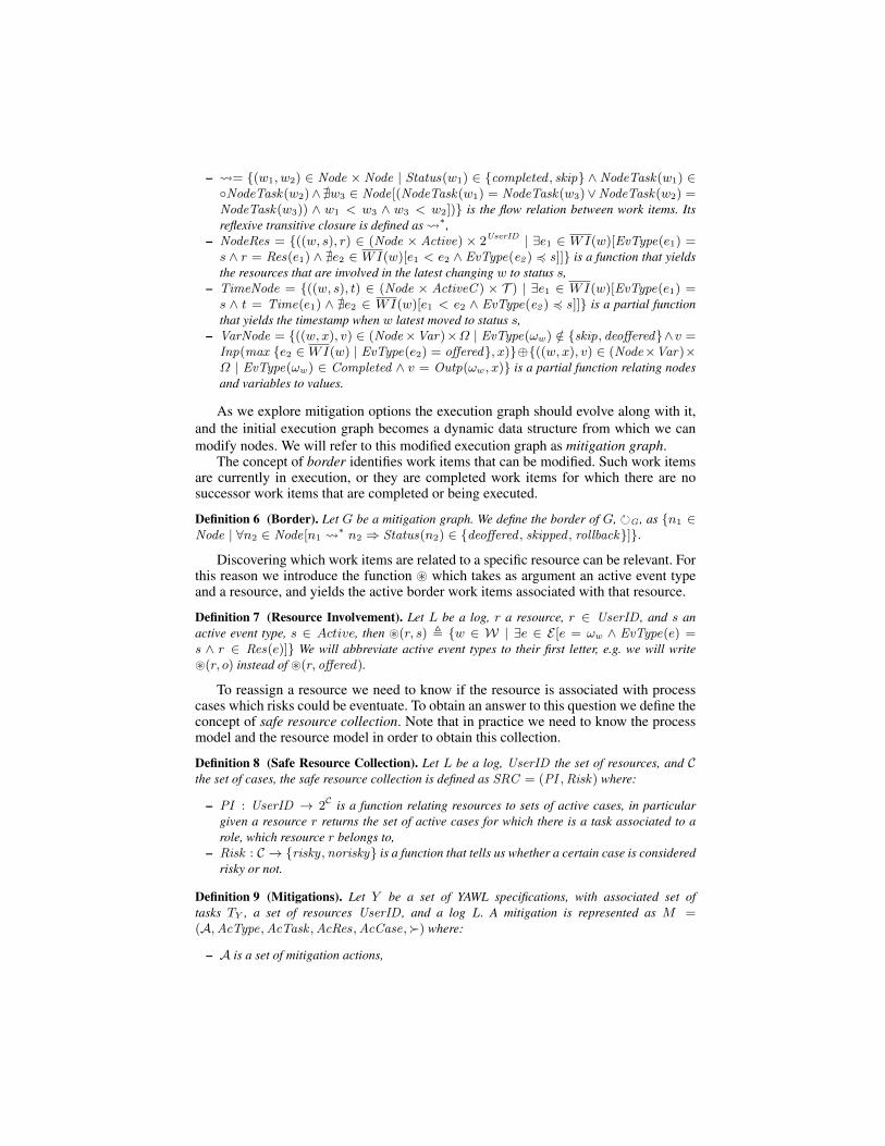
As we explore mitigation options the execution graph should evolve along with it,and the initial execution graph becomes a dynamic data structure from which we canmodify nodes. We will refer to this modified execution graph as mitigation graph.
The concept of border identifies work items that can be modified. Such work itemsare currently in execution, or they are completed work items for which there are nosuccessor work items that are completed or being executed.
Definition 6 (Border). Let G be a mitigation graph. We define the border of G, G , as n1 ∈Node | ∀n2 ∈ Node[n1
∗ n2 ⇒ Status(n2) ∈ deoffered , skipped , rollback].
Discovering which work items are related to a specific resource can be relevant. Forthis reason we introduce the function ~ which takes as argument an active event typeand a resource, and yields the active border work items associated with that resource.
Definition 7 (Resource Involvement). Let L be a log, r a resource, r ∈ UserID , and s anactive event type, s ∈ Active, then ~(r, s) , w ∈ W | ∃e ∈ E [e = ωw ∧ EvType(e) =s ∧ r ∈ Res(e)] We will abbreviate active event types to their first letter, e.g. we will write~(r, o) instead of ~(r, offered).
To reassign a resource we need to know if the resource is associated with processcases which risks could be eventuate. To obtain an answer to this question we define theconcept of safe resource collection. Note that in practice we need to know the processmodel and the resource model in order to obtain this collection.
Definition 8 (Safe Resource Collection). Let L be a log, UserID the set of resources, and Cthe set of cases, the safe resource collection is defined as SRC = (PI ,Risk) where:
– PI : UserID → 2C is a function relating resources to sets of active cases, in particulargiven a resource r returns the set of active cases for which there is a task associated to arole, which resource r belongs to,
– Risk : C → risky ,norisky is a function that tells us whether a certain case is consideredrisky or not.
Definition 9 (Mitigations). Let Y be a set of YAWL specifications, with associated set oftasks TY , a set of resources UserID , and a log L. A mitigation is represented as M =(A,AcType,AcTask ,AcRes,AcCase,) where:
– A is a set of mitigation actions,

– AcType : A → deoffer , deallocate, destart , offer , allocate, start , rollback , skip, is afunction relating actions to types of mitigation,
– AcTask : A → TY is a function relating actions to tasks,– AcRes : A UserID is a partial function relating actions to resources,– AcCase : A → C is a function relating actions to cases,– ⊆ A×A is a total ordering on mitigation actions indicating the order in which they need
to be performed. We refer to this total ordering as the mitigation sequence.
The insertion of a new mitigation action a /∈ A into mitigation M , can be expressedas addMit(M,a, et, t, r, c) , (A ∪ a,AcType ∪ (a, et),AcTask ∪ (a, t),AcRes ∪(a, r),AcCase ∪ (a, c), ∪(x, a) | x ∈ A).
Now we are in a position to introduce the mitigation actions. For each action wewill provide a short description of its behavior; we will quantify its cost and specifythe precondition(s) required for its application. All these actions are executed in thecontext of a mitigation M . As soon as a risk is detected we collect the log L containingall process cases. This log is used to generate an execution graph G′, that we refer to asthe original execution graph. It is used as a reference for comparison with the originalstatus of the system. The effects of mitigations actions are explored, though not yetapplied, during execution of the mitigation algorithm, and hence they are performed ona clone of the original execution graph which we will refer to as G.
Throughout the remainder of this section G′ is the original execution graph, G themitigation graph in use, and c ∈ C is a case. Moreover, whenever a node is modified,we need to store the time this modification occurred. In order to capture the time, weuse function curr().
A mitigation is a sequence of mitigation actions. Below we describe the mitigationactions supported by the PRSA algorithm.
Deoffer This action deoffers a task from a resource to whom the task was offered.We can execute deOff (c,G,M) as described in Algorithm 1 if there is a work itemx ∈ G such that x is an offered work item. The cost of this action was set to one andthis action serves as a reference for the cost of the other actions.
Algorithm 1: Deoffer Taskfunction deOff (Case c, Mitigation GraphG, MitigationM );Output: Mitigation GraphG, MitigationMbegin
n⇐ Any(x ∈ G | Status(x) = offered);if n 6=⊥ then
r ⇐ Any(NodeRes(n, offered));if |NodeRes(n, offered)| > 1 then
et⇐ offered ;TimeNode ⇐ TimeNode ⊕ ((n, offered), curr());NodeRes ⇐ NodeRes ⊕ ((n, offered),NodeRes(n, offered) \ r);
elseet⇐ deoffered ;TimeNode ⇐ (n, offered) –/TimeNode;NodeRes ⇐ NodeRes(n, offered) –/NodeRes;VarNode ⇐ (n, v) | VarNode(n, v) ∈ Ω –/TimeNode;
Status ⇐ Status ⊕ (n, et);M ⇐ addMit(M,NewAction(), deoffer ,NodeTask(n), r, c);
return (G,M)
Deallocate This action deallocates a task from the resource to whom the task wasallocated. If there is a work item x ∈ G such that x is an allocated work item,

we can execute deAll(c,G,M) as described in Algorithm 2. We set the cost of thisaction to two, since considering the progress status of a work item, deallocating a workitem should be more “expensive” than deoffering it. In the Payment subprocess thisaction could be used to mitigate the approval fraud risk. The work item of “ApproveShipment Payment Order” can be deallocated from the resource to whom this workitem is allocated when the risk is detected, since this resource approved another orderfor the same customer in the past.
Algorithm 2: Deallocate Taskfunction deAll(Case c, Mitigation GraphG, MitigationM );Output: Mitigation GraphG, MitigationMbegin
n⇐ Any(x ∈ G | Status(x) = allocated);if n 6=⊥ then
r ⇐ Any(NodeRes(n, allocated));Status ⇐ Status ⊕ (n, offered);NodeRes ⇐ (n, allocated) –/NodeRes;TimeNode ⇐ (n, allocated) –/TimeNode;M ⇐ addMit(M,NewAction(), deallocate,NodeTask(n), r, c);
return (G,M)
Destart This action brings an already started work item back to the state allocatedand allocates it to the resource who started it. We can execute deSta(c,G,M), as de-scribed in Algorithm 3, if there is a work item x ∈ G such that x is a started workitem. For this action we set the cost to three as destarting a work item requires more ef-fort than deallocating a work item. The destart action may be used to mitigate the samerisk as the deallocate action. This action may be used to destart a resource who neverapproved an order for the current customer from another work item, reducing this waythe probability of allocating the work item to a resource who approved the ShipmentPayment Order in the past.
Algorithm 3: Destart Taskfunction deSta(Case c, Mitigation GraphG, MitigationM );Output: Mitigation GraphG, MitigationMbegin
n⇐ Any(x ∈ G | Status(x) = started);if n 6=⊥ then
r ⇐ Any(NodeRes(n, started));Status ⇐ Status ⊕ (n, allocated);NodeRes ⇐ (n, started) –/NodeRes;TimeNode ⇐ (n, started) –/TimeNode;M ⇐ addMit(M,NewAction(), destart,NodeTask(n), r, c);
return (G,M)
Offer This action offers a work item to a resource to whom the task is not currentlyoffered, either because it is not yet part of the set of resources to whom the task iscurrently offered, or because the task is currently deoffered . Given a function D thatrelates tasks to the set of resources to whom their work items can be offered, we canexecute off (D, c,G,G′,M), as described in Algorithm 4, if there is a work item x ∈G such that x is an offered or deoffered work item, and this work item is an offered ,allocated or started work item in the execution graph G′. This action has a cost of one,the same as the offer action.

Algorithm 4: Offer Taskfunction off (Distribution SetD, Case c, Mitigation GraphG, Execution GraphG′, MitigationM );Output: Mitigation GraphG, MitigationMbegin
n⇐ Any(x ∈ G | StatusG(x) ∈ offered, deoffered ∧ StatusG′ (x) ∈ Active);r ⇐⊥;if n 6=⊥ then
r ⇐ Any(D(NodeTask(n)) \ NodeResG(n, offered) ∪ NodeResG′ (n, offered));
if r 6=⊥ thenif StatusG = deoffered then
StatusG ⇐ StatusG ⊕ (n, offered);VarNodeG ⇐ TimeNodeG ∪ VarNodeG′ (n);TimeNodeG ⇐ TimeNodeG ∪ ((n, offered), curr());NodeResG ⇐ NodeResG ∪ ((n, offered),NodeResG(n, offered) ∪ r);
elseTimeNodeG ⇐ TimeNodeG ⊕ ((n, offered), curr());NodeResG ⇐ NodeResG ⊕ ((n, offered),NodeResG(n, offered) ∪ r);
M ⇐ addMit(M,NewAction(), offer ,NodeTaskG(n), r, c);
return (G,M)
Allocate This action reallocates a work item that was deallocated before (and stillhas not been allocated) to a resource to whom the task was not allocated when thedeallocation took place. We can execute all(c,G,G′,M), as described in Algorithm 5,if there is a work item x ∈ G such that x is an offered work item, and x is originally anallocated or started work item. This action has a cost of minus one. The reason behindthis is quite simple. Since this action can only be executed if we previously executed adeallocation, these two actions can be seen as a unique action that change the resourceinvolved with the work item. For example this action can be used once we deallocateda resource from a work item of the “Approve Shipment Payment Order” task. Then thisaction allocates the same work item to another resource who may not have approved anorder for the same customer in the past.
Algorithm 5: Allocate Taskfunction all(Case c, Mitigation GraphG, Execution GraphG′, MitigationM );Output: Mitigation GraphG, MitigationMbegin
n⇐ Any(x ∈ G | StatusG(x) = offered ∧ StatusG′ (x) ∈ allocated, started);r ⇐⊥;if n 6=⊥ then
r ⇐ Any(NodeResG(n, offered) \ NodeResG′ (n, allocated));
if r 6=⊥ thenStatusG ⇐ StatusG ⊕ (n, allocated);NodeResG ⇐ NodeResG ∪ ((n, allocated), r);TimeNodeG ⇐ TimeNodeG ∪ ((n, allocated), curr());M ⇐ addMit(M,NewAction(), allocate,NodeTaskG(n), r, c);
return (G,M)
Start This action restarts a work item that was previously destarted (and has not yetbeen restarted) and associates it with a different resource from the one who started thetask. We can execute sta(c,G,G′,M), as described in Algorithm 6, if there is a workitem x ∈ G such that x is an allocated work item, and x is originally a started workitem. The cost of this action is minus one, and the reasoning is similar to that used forthe allocate action.

Algorithm 6: Start Taskfunction sta(Case c, Mitigation GraphG, Execution GraphG′, MitigationM );Output: Mitigation GraphG, MitigationMbegin
n⇐ Any(x ∈ G | StatusG(x) = allocated ∧ StatusG′ (x) = started);r ⇐⊥;if n 6=⊥ then
r ⇐ NodeResG(n, allocated) \ NodeResG′ (n, started);if r 6=⊥ then
StatusG ⇐ StatusG ⊕ (n, started);NodeResG ⇐ NodeResG ∪ ((n, started), r);TimeNodeG ⇐ TimeNodeG ∪ ((n, started), curr());M ⇐ addMit(M,NewAction(), start,NodeTaskG(n), r, c);
return (G,M)
Rollback This action returns a completed work item to the status of unoffered.We can execute rollbackTask(c,G) if there is a work item x ∈ G such that x is acompleted work item. Its operationalization is described in Algorithm 7. The rollbackaction restores the case to a consistent status where the execution of a given work itemnever happened. A compensation routine can be associated with a task, so that it istriggered when the task is rolled back. The idea of this compensation routine is to dealwith elements outside the control of the workflow engine (e.g. returning the moneyto a client after their payment has been rolled back). The rollback action is our mostpowerful action and has a cost of nine, obtained by adding the absolute values of allthe actions introduced until now. In our Payment subprocess, we could use this actionwhen we execute a large number of updates on the same Payment Order.
Algorithm 7: Rollback Taskfunction rollbackTask (Case c, Execution GraphG, MitigationM );Output: Execution GraphG, MitigationMbegin
n1 ⇐ Any(x ∈ G | StatusG(x) ∈ Completed);if n1 6=⊥ then
foreach n2 ∈ NodeG doif n1
∗G n2 then StatusG ⇐ StatusG ⊕ (n2, rollback);
StatusG ⇐ StatusG ⊕ (n1, rollback);M ⇐ addMit(M,NewAction(), rollback ,NodeTaskG(n1),⊥, c);
return (G,M)
Skip This action marks an unoffered and skippable task as ‘to be skipped’. If thereexists a task t ∈ skippable which does not have any work item active or completed,and there not exists a mitigation action a ∈ A which skipped task t for case c, thenwe define skipTask(c,G) as described in Algorithm 8. To limit the use of this action,since this action may produce inconsistency in the data, we decided to assign a costof nine. The utility of this action can be seen in two situations when we consider ourrunning example. The first situation is the order unfulfillment. In this case, to preventthe reiterated execution of an update, we may decide to skip the “Update ShipmentPayment Order” task. The second situation is the overtime process risk. In this case wemay decide to skip some tasks in order to complete the process in time.
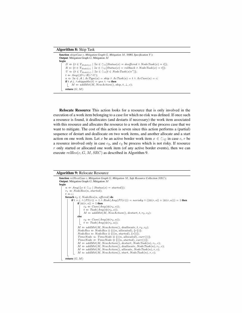
Algorithm 8: Skip Taskfunction skip(Case c, Mitigation GraphG, MitigationM , YAWL Specification Y );Output: Mitigation GraphG, MitigationMbegin
D ⇐ t ∈ TModel(c) | ∃x ∈ G [Status(x) = deoffered ∧ NodeTask(x) = t];R ⇐ t ∈ TModel(c) | ∃x ∈ G [Status(x) = rollback ∧ NodeTask(x) = t];U ⇐ t ∈ TModel(c) | ∃x ∈ G [t ∈ NodeTask(x)∗];t⇐ Any((D ∪ R) ∩ U);a⇐ ∃a ∈ A | AcType(a) = skip ∧ AcTask(a) = t ∧ AcCase(a) = c;if t 6=⊥ ∧skippable(t) = yes ∧ ¬a then
M ⇐ addMit(M,NewAction(), skip, t,⊥, c);
return (G,M)
Relocate Resource This action looks for a resource that is only involved in theexecution of a work item belonging to a case for which no risk was defined. If once sucha resource is found, it deallocates (and destarts if necessary) the work item associatedwith this resource and allocates the resource to a work item of the process case that wewant to mitigate. The cost of this action is seven since this action performs a (partial)sequence of destart and deallocate on two work items, and another allocate and a startaction on one work item. Let x be an active border work item x ∈ G in case c, r bea resource involved only in case c2, and c2 be process which is not risky. If resourcer only started or allocated one work item (of any active border events), then we canexecute relRes(c,G,M,SRC ) as described in Algorithm 9.
Algorithm 9: Relocate Resourcefunction relRes(Case c, Mitigation GraphG, MitigationM , Safe Resource Collection SRC );Output: Mitigation GraphG, MitigationMbegin
n⇐ Any(x ∈ G | Status(x) = started);r1 ⇐ NodeRes(n, started);t⇐⊥;foreach r2 ∈ NodeRes(n, offered) do
if t =⊥ ∧ |PI (r)| = 1∧Risk(Any(PI (r))) = norisky ∧ (|~(r, s)|+ |~(r, a)|) = 1 thenif |~(r, s)| = 1 then
c2 ⇐ Case(Any(~(r2, s));t⇐ Task(Any(~(r2, s));M ⇐ addMit(M,NewAction(), destart, t, r2, c2);
elsec2 ⇐ Case(Any(~(r2, a));t⇐ Task(Any(~(r2, a));
M ⇐ addMit(M,NewAction(), deallocate, t, r2, c2);NodeRes ⇐ NodeRes ⊕ ((n, allocated), r);NodeRes ⇐ NodeRes ⊕ ((n, started), r);TimeNode ⇐ TimeNode ⊕ ((n, allocated), curr());TimeNode ⇐ TimeNode ⊕ ((n, started), curr());M ⇐ addMit(M,NewAction(), destart,NodeTask(n), r1, c);M ⇐ addMit(M,NewAction(), deallocate,NodeTask(n), r1, c);M ⇐ addMit(M,NewAction(), allocate,NodeTask(n), r, c);M ⇐ addMit(M,NewAction(), start,NodeTask(n), r, c);
return (G,M)

4 Evaluation
We implemented the PRSA algorithm as a custom service in the YAWL system.4 Weextended the YAWL system as it is built on a service-oriented architecture, which fa-cilitates the addition of new services; it is open-source, which facilitates its distributionamong academics and practitioners; and as the underlying YAWL language providescomprehensive supports for the workflow patterns [18].
The risk mitigation service interacts with the risk detection service5 that we devel-oped previously [11], for the sake of identifying risks and computing their probabilities.It uses as input a reference to the process instance whose risks need to be mitigated, thecomplete YAWL specification for this instance, a log of the process (as extracted fromthe YAWL system), and a copy of the risk sensors associated with the process instance,as provided by the risk detection service. Modifications that a mitigation may introduceare communicated to the risk detection service, which recomputes the risk probabili-ties. The final solutions are returned to the user as recommendations. The one chosenby the user is then applied to the process instance under exam using the APIs providedby the YAWL engine. We implemented compensation actions associated with rolledback work items via the YAWL Worklet mechanism [18]. Accordingly, we equippedthe YAWL Editor with an interface to allow users to associate a Worklet containing acompensation action to a task. When an instance of this task is rolled back, the associ-ated Worklet is run as a separate process instance in the YAWL engine, so that from anengine perspective, the Worklet and its invoking processes are two distinct cases.
To prove the feasibility of our approach, we ran three experiments. First, we testedthe required time to mitigate the same set of risks on different process models. Second,we checked the dependency of the mitigation time on different variables. Third, wechecked the quality of the mitigations proposed on a specific process model.
For the first experiment, we selected four process models from real-life (see ap-pendix A), with a minimum of five tasks and a maximum of twenty tasks. The firstmodel (Process A) describes a film production process, carried out on a daily basis. Thisprocess is taken from a case study we conducted in collaboration with the AustralianFilm, Television and Radio School [24]. The other three models are subprocesses ofan order fulfillment process inspired by the VICS industry standard for logistics [28].The first of these processes (Process B) deals with the ordering, the second (Process C)deals with the payment for the goods and is the process we showed in Section 2, thethird process (Process D) deals with the delivery of the goods.
Next, we defined seven generic risk conditions on these processes (see appendix B).These conditions represent possible undesirable situations that may arise in a process,and relate to different process aspects such as data, resources and control-flow ele-ments. They are domain-independent so that we could define them on all four processmodels. The first condition detects a situation where two concurrent work items maynot complete in a desired order. The second one is used to detect a violation of thefour-eyes principle between parallel work items. The third one detects whether a timelimit is exceed when executing a loop. The fourth condition detects a possible delay
4 http://www.yawlfoundation.org5 http://www.yawlfoundation.org/prsa

with the execution of a work item. The fifth one detects the possibility that two concur-rent work items that should be executed by the same resource are actually allocated totwo different resources (a situation that is not possible to enforce with many workflowmanagement systems). The sixth one detects a delay with the execution of a portionof the process while the seventh one detects a data error, specifically if the data valuesproduced by two concurrent work items are not the same.
For each process model we generated a variant with a specific combina-tion of the above risk conditions. This led to a total of 180 process mod-els (not every risk identified could be applied to every process model), asfollows: 19 models with one risk condition, 40 models with two risk con-ditions, 50 with three risk conditions, 41 models with four risk conditions,
Process Size Variants Risks Mitigation time [sec] Candidatesavg/max min max avg min max avg
Process A 20 127 3.53 / 7 0.003 178.891 26.415 2 20,181 3,456Process B 5 7 1.71 / 3 0.001 0.033 0.015 3 54 32Process C 15 31 3.05 / 5 0.001 0.117 0.030 2 256 60.93Process D 5 15 2.13 / 4 0.004 0.929 0.170 2 553 78.2
Total 45 180 3.18 / 7 0.001 178.891 18.657 2 20,181 2,457
Table 1. Time and number of candidate solutions ex-plored to find the first solution.
22 process models with fiverisk conditions, seven pro-cess models with six riskconditions, and one processmodel with all seven riskconditions.
For each process modelwe ran ten tests and aver-aged the results. Each testwas executed on the first state of a process instance where all the risk conditions evalu-ated to true. For each group of tests on the same process model we measured the timerequired to obtain the first solution that mitigates all risks, and the number of candi-date solutions generated by the algorithm in order to obtain this solution. We performedthe tests on an Intel Core I5 M560 2.67GHz processor with 4GB RAM, running LinuxLubuntu v11.10.
Table 1 shows the results of this experiment. The second, third and fourth columnsshow the size (as number of tasks), the number of variants and the number of riskconditions for each of the four process models. The fifth and sixth columns show themitigation time required to find the first solution, and the number of candidate solutionsexplored to find such a solution. From this table we can observe that the algorithm takesat most 3 mins (179 secs) to mitigate multiple risks in a variant of Process A (this timingrefers to a combination of 5 risks for this process), though the average time is muchlower (19 secs across all models). It seems reasonable to assume that in most businessscenarios mitigation times in the order of a few minutes are acceptable, compared tothe average time required to perform a task, and thus the average duration of a processinstance. For example, let us assume an average duration of 24 hours for the Paymentsubprocess, with a new task being executed every 30 mins. Let us also assume that wesample the risk conditions every 5 mins. This means we have up to 6 mins to mitigateall identified risks before a new task is executed which may change the risk conditions.
Table 1 also shows that the algorithm needs to explore a very large number of can-didate solutions to find the first solution (2,456 solutions on average across all models).While it is not fair to compare the computation power of a machine to that of humans,this result highlights the complexity of finding a solution. It is reasonable to think that

many of these candidate solutions explored by the algorithm would also need be evalu-ated by a human in order to find the right solution.
R² = 0.07
0.0020.0040.0060.0080.00
100.00120.00140.00160.00180.00200.00
0 0.1 0.2 0.3 0.4 0.5 0.6 0.7 0.8 0.9
Time vs Risks/Process tasks
R² = 0.7411
0.00
0.00
0.01
0.10
1.00
10.00
100.00
1000.00
10000.00
0 2 4 6 8 10
Time vs #Tasks in risk condition
Fig. 3. Correlation between time and a) risks/tasks ratio, b) tasks in risk conditions.
In the second experiment, we investigated the factors affecting the performance ofthe algorithm. One would think that the mitigation time is proportional to the number ofrisks defined in a process model, and to the model size itself. The larger the number ofrisks and/or the model size, the longer it should take to mitigate such risks. However thedata we extrapolated from Table 1 does not confirm this hypothesis. For example, the 21variants of Process A with 5 risks have mitigation times ranging from 3.3 to 179 secs,despite their sizes and number of risks being the same. To verify that the mitigation timeis not sensitive to the number of risks, nor to the process size, we plotted the correlationbetween the mitigation time and the ratio risks/process size in Figure 3a (the solid line isthe linear regression of the points). The low value of the coefficient of determination R2
(0.07) confirms this intuition. We then checked the correlation between the mitigationtime and the number of tasks used in risk conditions. The intuition is that the morework items of these tasks are pending in a given state of the process instance, the largerthe number of possible mitigation actions. The corresponding scatter plot is shown inFigure 3b, which indeed confirms this intuition (R2 = 0.74).
Finally, we checked the feasibility of the solutions proposed by the algorithm,when mitigating the domain-specific risks associated with the Payment subprocess (cf.Section 2). We recall that two of these risks (overtime process and order unfulfill-ment) are detected when the associated probability, obtained by analyzing historicaldata, exceeds a tolerance threshold, whereas the third risk (approval fraud) involvesa complex risk condition. We considered the first state of an instance of the Paymentsubprocess when all three risks are active. This occurs after executing “Update ship-ment payment order” for the third time, once task “Approve shipment payment or-der” has been allocated to a resource who has already executed this task in the past.
Solutions [at 1 min] 1 2 3 4 5Overtime Process + + + + +Approval Fraud + + + + +
Order Unfulfillment + + ± ± −Cost 50 50 40 40 19
Table 2. Payment subprocessmitigation.
To obtain a small number of solutions, we stoppedthe algorithm after one min of execution. In this time-frame, five solutions were retrieved. For each solution,Table 2 reports whether the solution mitigates each ofthe three risks, and the cost of the solution in termsof mitigation actions performed on the initial processinstance. In particular, a “−” indicates a risk not mit-

igated, a “+” indicates a risk mitigated (with risk probability lower than the specificthreshold if the condition depends on the risk probability), and a “±” indicates a riskmitigated whose condition cannot be computed for lack of information, i.e. some of thevariables used in the risk condition are null. We recall that the algorithm prioritizes asolution whose risk is mitigated by computing the risk condition, than a solution whoserisk is mitigated because the respective condition cannot be computed.
The five solutions identified are pairwise mutually non-dominating. Solutions 1 and2 are dominated by solutions 3, 4 and 5 cost-wise, but dominate these solutions w.r.t.the mitigation of the order unfulfillment risk. Solution 5 dominates solutions 3 and4 cost-wise but is dominated by these two solutions w.r.t. the mitigation of the orderunfulfillment risk.
Let us briefly examine the mitigations performed by the five solutions (see ap-pendix C). The first four solutions mitigate the approval fraud by deallocating the re-source that was allocated “Approve shipment payment order”, while solution 5 addi-tionally allocates the work item to a resource who did not execute this task for the samecustomer in the past. All these mitigations are feasible, though the one provided by so-lution 5 is more robust, since there is no risk that the task gets allocated to a resourcewho has already executed it. The order unfulfillment risk is mitigated by solutions 1 and2 through rolling back the work item of task “Update shipment payment order” (whichleads to a deoffer of the work item of task “Approve shipment payment order” thatcomes afterwards). Solutions 3 and 4 do this too but also mark this task ‘to be skipped’preventing a possible re-execution of it. This action sets to null the risk variables asso-ciated with this task that retrieve the number of executions and its estimated remainingtime making the risk mitigated but not computable. Thus, while all four solutions arefeasible, we would prioritise the first two since these ensure that the risk probabilityhas actually dropped below the threshold. Finally, all solutions differ in the way theymitigate the overtime process risk. Each of them skips a different task among those notyet executed (for simplicity, all of them have the same estimated duration). Despite thefact that all these solutions are feasible, only the mitigation proposed by solution 3 isinteresting since it proposes to skip tasks “Update Shipment Payment Order” and “Ap-prove Shipment Payment Order” avoiding this way that the loop is taken again. In otherwords, it prevents the order to undergo further updates, and subsequent approvals.
5 Related Work
Risk mitigation is an essential step in the risk management process [27]. Several riskanalysis methods such as OCTAVE [4], CRAMM [7] and CORAS [21] describe riskmitigation guidelines. Although helpful, these guidelines are too generic and no sup-port is offered on how they could be operationalized. Similarly, the academic literaturerecognizes the importance of mitigating process-related risks, though it focuses moreon risk-aware BPM methodologies than on concrete algorithms for automating riskmitigation. For a comprehensive comparison of these methodologies, we refer to [11].A well known example is the ROPE (Risk-Oriented Process Evaluation) methodology[16]. ROPE is concerned with threats to the resources required for process executions.If a required resource becomes unavailable, pre-planned countermeasures and recov-

ery procedures are manually enacted to handle the fault. These procedures are definedand validated via a simulator at design-time; enactment at runtime is designated to a‘responsible person’, that is, the mitigation and recovery operations are not automated.
Various frameworks have been proposed for the dynamic adaptation of process in-stances. For example, ADEPT [12] supports adding, deleting and changing the sequenceof tasks at both the model and instance levels, however such changes must be achievedvia manual intervention by an administrator. AgentWork [23] provides the ability tomodify process instances by dropping and adding individual tasks based on events andrules. CBRFlow [29] uses case-based reasoning to support runtime adaptation by allow-ing users to annotate rules during process execution. CEVICHE [17] is a service-basedframework that uses the AO4BPEL (Aspect-Oriented for BPEL) language [9] to pro-vide an option for skipping or reallocating tasks to other services in an ad-hoc manner.While these approaches could be used for risk mitigation purposes, they do not provideany help for the identification of which particular mitigation actions should be used.The YAWL Worklet Service [3] provides each task of a process instance with the abil-ity to be associated with an extensible repertoire of actions (‘drop-in’ processes), oneof which is contextually and dynamically bound to the task at runtime. It also supportscapabilities for dynamically detecting and handling runtime exceptions, however the ap-proach is generic and not specifically designed for risk detection and mitigation. Also anew situation cannot automatically be dealt with but requires a workflow administratorto intervene.
Our work is also related to operational support in process mining [1]. Operationalsupport deals with the analysis of current and historical execution data, with the aimto predict future states of a running process instance, and provide recommendations toguide the user in selecting the next activity to execute based on certain objectives. Forexample, the approach for cycle time prediction in [2] could be, with the opportunemodifications, adapted for risk prediction. Using this approach it would be possibleto estimate the probability of an overtime risk and suggest the next steps the currentinstance should take in order to keep this risk under control. The application of thisapproach unfortunately requires that the process model captures all the possible mitiga-tion actions as normal activities, i.e. as control-flow alternatives. For instance, if a taskcan be skipped, there should be a path without that task that leads to the end node ofthe process model. This may drastically increase the complexity of the process model.Moreover, this approach would not be applicable to capture mitigation operations onresources (i.e. deallocating a resource) or on task states (e.g. suspending a task). Thatsaid, more in general, our approach can be seen as a possible provider for operationsupport, and could thus be integrated in process mining environments like ProM.6
Our work provides recommendations to users as to which mitigation actions can beapplied to the specific context at hand. As such, it shares commonalities with recom-mendation and decision support systems (DSS). Alter [5] states that the focus of suchsystems should be towards improving decision making within work systems, rather thanexternalizing support. This view is shared by our technique, which provides an exten-sion for existing process-aware information systems, rather than a separate standalonetool. As such, it may be considered a member of the domain known as Group Decision
6 http://processmining.org

Support Systems, which facilitate task support in group environments. The conjunc-tion of our work and DSS can be demonstrated via Alter’s twenty-four work systemprinciples [6], which may be used to analyze the capabilities of systems, using com-monly understood terminology. In particular, our work meets principles #5 (encourageappropriate use of judgement), #6 (control problems at their source), #9 (match workpractices with participants), #13 (provide information where it will affect action), #14(protect information from inappropriate use), #22 (minimize unnecessary risks) and #24(maintain the ability to adapt, change and grow). In addition, our work provides all fourfeatures associated with a DSS’s ability to improve practice, as identified in a surveyof seventy studies within the healthcare domain: (a) decision support provided auto-matically as part of workflow; (b) decision support delivered at the time and locationof decision making; (c) actionable recommendations provided; and (d) computer based[20].
The mitigation operations we perform on resources share commonalities with taskrescheduling systems, which become particularly important in those domains whereappointment-based task executions are critical (e.g. healthcare). For example, a systemis presented in [22] that supports the integration of unscheduled and scheduled taskswithin a process instance by interfacing a workflow engine with individual user calen-dars maintained by MS Exchange Server. A similar, though more generic, approach isencapsulated in the YAWL Scheduling Service [25]. Another approach, by Eder et al.[14], focuses on the creation of personal schedules for each user so that a workflow en-gine, when making decisions about work assignment, can take into account informationabout a user’s time constraints and availability to perform particular tasks.
In previous work [15] we explored the use of dominance-based MOSA for auto-matically fixing behavioral errors in process models, at design-time. Our work on riskmitigation can thus be seen as an adaptation of that idea to run-time aspects, since weaim to improve running process instances. Besides their distinct aims, the main differ-ence between the two approaches is that for correcting behavioral errors we definedthree objective functions capturing the structural and behavioral similarity of a solu-tion to the incorrect model, whereas in risk mitigation the number and type of objectivefunctions depends on which risks are active in a given state of a process instance.
6 Conclusion
This paper contributes a concrete technique for the automatic mitigation of process-related risks at run-time. The technique requires as input an executable process modeland a set of associated risk conditions. At run-time, when one or more risk conditionsevaluate to true, a process administrator can launch our technique to mitigate the iden-tified risks and bring the process instance back to a safe state. This is achieved by gen-erating a set of possible mitigations that change the current instance in order to bringthe likelihood of the identified risks below a tolerance level. These mitigation actionsare not performed directly on the instance under consideration. Rather, their effects aresimulated and those solutions that mitigate the most risks in a given timeframe, areproposed as recommendations to the process administrator.

The mitigation actions are determined via a dominance-based MOSA algorithm.This choice allows us to explore the solution space as widely as possible, avoidinglocal optima. In essence, each risk is treated as an objective function whose likelihoodneeds be minimized. The objective is reached as soon as the likelihood goes below thetolerance value for that particular risk. Mitigation actions affect various aspects of aprocess, such as task execution and resources utilization. To the best of our knowledge,this is the first time that process-related risks can be mitigated automatically.
The technique was implemented in the YAWL system and its performance evaluatedwith real-life process models. The tests show that on the analyzed process models a setof possible solutions can be found in a matter of seconds, or within a few minutes inthe worst case, and that in all cases the associated risks are mitigated. We expect thistechnique to reduce the effort and time required by process administrators to understandwhat mitigation actions are feasible based on a particular state of the system. That said,we still need to validate the feasibility and appropriateness of the proposed mitigationactions with domain experts. We plan to do so by comparing the solutions obtained withour algorithm with those proposed by them. We also plan to improve the explorationof the solution space by prioritizing the mitigation of those risks that have the highestimpact on the process objectives. In fact, currently all risks are treated alike whereasin reality this might not be the case. Finally, the algorithm could also be extended toprioritize certain mitigation actions based on how these have been ranked by the usersin previously mitigated instances.
Acknowledgments We thank Peter Hughes for his valuable comments on the mitiga-tion operations. This research is funded by the ARC Discovery Project “Risk-awareBusiness Process Management” (DP110100091).
References
1. W.M.P. van der Aalst. Process Mining - Discovery, Conformance and Enhancement of Busi-ness Processes. Springer, 2011.
2. W.M.P. van der Aalst, M.H. Schonenberg, and M. Song. Time prediction based on processmining. Information Systems, 36(2):450–475, 2011.
3. M. Adams, A.H.M. ter Hofstede, W.M.P. van der Aalst, and D. Edmond. Dynamic, extensibleand context-aware exception handling for workflows. In CoopIS, volume 4803 of LNCS,pages 95–112. Springer, 2007.
4. C.J. Alberts and A.J. Dorofee. OCTAVE criteria, version 2.0. Technical Report CMU/SEI-2001-TR-016, Carnegie Mellon University, 2001.
5. S. Alter. A work system view of DSS in its fourth decade. DSS, 38, December 2004.6. S. Alter and R. Wright. Validating work system principles for use in systems analysis and
design. In Proceedings of the 30th International Conference on Information System (ICIS2010). AIS eLibrary, 2010.
7. B. Barber and J. Davey. The use of the CCTA Risk Analysis and Management MethodologyCRAMM in health information systems. In MEDINFO. North Holland Publishing, 1992.
8. Basel Committee on Bankin Supervision. Basel II - International Convergence of CapitalMeasurement and Capital Standards, 2006.
9. A. Charfi and M. Mezini. AO4BPEL: An aspect-oriented extension to BPEL. World WideWeb, 10(3):309–344, 2007.

10. International Electrotechnical Commission. IEC 61025 Fault Tree Analysis (FTA), 1990.11. R. Conforti, G. Fortino, M. La Rosa, and A.H.M. ter Hofstede. History-aware, real-time risk
detection in business processes. In CoopIS, volume 7044 of LNCS. Springer, 2011.12. P. Dadam and M. Reichert. The ADEPT project: a decade of research and development for
robust and flexible process support. CSRD, 23:81–97, 2009.13. M. Dumas, W.M.P. van der Aalst, and A.H.M. ter Hofstede. Process-Aware Information
Systems: Bridging People and Software through Process Technology. Wiley & Sons, 2005.14. Johann Eder, Horst Pichler, Wolfgang Gruber, and Michael Ninaus. Personal schedules
for workflow systems. In Arthur ter Hofstede and Mathias Weske, editors, Business Pro-cess Management, volume 2678 of Lecture Notes in Computer Science, pages 1018–1018.Springer Berlin / Heidelberg, 2003.
15. M. Gambini, M. La Rosa, S. Migliorini, and A.H.M. ter Hofstede. Automated error correc-tion of business process models. In BPM, volume 6896 of LNCS. Springer, 2011.
16. G. Goluch, S. Tjoa, S. Jakoubi, and G. Quirchmayr. Deriving resource requirements applyingrisk-aware business process modeling and simulation. In ECIS. AISeL, 2008.
17. G. Hermosillo, L. Seinturier, and L. Duchien. Using complex event processing for dynamicbusiness process adaptation. In SCC, pages 466 –473. IEEE, 2010.
18. A.H.M. ter Hofstede, W.M.P. van der Aalst, M. Adams, and N. Russell, editors. ModernBusiness Process Automation: YAWL and its Support Environment. Springer, 2010.
19. W.G. Johnson. MORT - The Management Oversight and Risk Tree. U.S. Atomic EnergyCommission, 1973.
20. Kensaku Kawamoto, Caitlin A Houlihan, E Andrew Balas, and David F Lobach. Improv-ing clinical practice using clinical decision support systems: a systematic review of trials toidentify features critical to success. British Medical Journal, 330(7494), April 2005.
21. M.S. Lund, B. Solhaug, and K. Stølen. Model-Driven Risk Analysis - The CORAS Approach.Springer, 2011.
22. Ronny Mans, Nick Russell, Wil van der Aalst, Arnold Moleman, and Piet Bakker. Schedule-aware workflow management systems. In Kurt Jensen, Susanna Donatelli, and MaciejKoutny, editors, Transactions on Petri Nets and Other Models of Concurrency IV, volume6550 of Lecture Notes in Computer Science, pages 121–143. Springer Berlin / Heidelberg,2010.
23. R. Muller, U. Greiner, and E. Rahm. AgentWork: a workflow system supporting rule-basedworkflow adaptation. Data & Knowledge Engineering, 51(2):223–256, 2004.
24. C. Ouyang, M. La Rosa, A.H.M. ter Hofstede, M. Dumas, and K. Shortland. Toward web-scale workflows for film production. IEEE, Internet Computing, 12(5):53–61, 2008.
25. C. Ouyang, M.T. Wynn, J-C. Kuhr, M. Adams, T. Becker, A.H.M. ter Hofstede, and C. Fidge.Workflow support for scheduling in surgical care processes. In ECIS.
26. K.I. Smith, R.M. Everson, J.E. Fieldsend, C. Murphy, and R. Misra. Dominance-based mul-tiobjective simulated annealing. IEEE TEC, 12(3):323–342, 2008.
27. Standards Australia and Standards New Zealand. Standard AS/NZS ISO 31000, 2009.28. Voluntary Interindustry Commerce Solutions Association. Voluntary Inter-industry Com-
merce Standard (VICS). http://www.vics.org. Accessed: June 2011.29. B. Weber, W. Wild, and R. Breu. CBRFlow: Enabling adaptive workflow management
through conversational case-based reasoning. In ECCBR, volume 3155 of LNCS. Springer,2004.

A Process Models
In this section we describe the business process models used for testing our approach.
A.1 Process A: Film Production Process
The process model in Figure 4 show the Film Production process [24]. This processstarts with the collections of documents produced during the pre-production phase.These documents are collected during the execution of Input Cast List, Input CrewList, Input Location Notes and Input Shooting Schedule. Once all documents are col-lected the process is carried out on a daily basis, following two parallel paths. The firstfocuses on producing a “call sheet”. A call sheet is a schedule for a particular day. Itis produced by the Production Office and delivered to all cast and crew one day in ad-vance. The second path focuses on the technical part of the production, producing logof activities and technical notes. In particular the tasks Fill Out Continuity Report andFill Out Continuity Daily Report are executed by the Continuity person, task Fill OutSound Sheets is executed by Sound Recordist, task Fill Out Camera Sheets is executedby Camera Assistant, and task Fill Out AD Report is executed by 2nd Assistant Di-rector. Once these five activities are completed a daily progress report is generated inCreate DPR and distributed to the Producer and Executive Producer in Distribute DPR.
Fig. 4. Film Production Process (using YAWL [18] notation).

A.2 Process B: Ordering Process
The process model in Figure 5 show the Ordering subprocess of the Order Fulfilmentprocess. This process deals with the placing of an purchase order. The process startwith the creation of a purchase order, carried out by a Process Order Manager (CreatePurchase Order task), and need to be approved by a Senior Supply Officer (ApprovePurchase Order task). Once an order is approved it can be modified and in this caseneed to be approved again, or confirmed by the same Process Order Manager whocreated it. If an order is not approved within three days it is automatically cancelled.
Fig. 5. Order Fulfilment Process: Ordering Subprocess (using YAWL [18] notation).
A.3 Process C: Payment Process
The process model in Figure 6 show the Payment subprocess of the Order Fulfil-ment process. This process starts after the freight has been picked up by a carrier anddeals with the shipment and freight payment executed in parallel. The freight paymentwhether required starts with the production of a freight invoice done by a Supply Ad-min Officer and ends with the processing of the freight payment. During the paymentof shipment costs, first a Shipment Invoice is produced for costs related to a specific or-der. If payment has been made in advance, a Finance Officer simply issues a ShipmentRemittance Advice to the customer specifying the amount paid. Otherwise, the FinanceOfficer issues a Shipment Payment Order, which requires approval by a Senior FinanceOfficer (a superior of the Finance Officer) who may request amendments be made by theFinance Officer that issued the Order. After the document is finalized and the customer

has paid, an Account Manager can process the payment. If the customer underpays, theAccount Manager issues a Debit Adjustment, the customer makes a further paymentand the payment is reprocessed. If a customer overpays, the Account Manager issues aCredit Adjustment. In the latter case and in the case of correct payment, the Paymentsubprocess completes.
Fig. 6. Order Fulfilment Process: Payment Subprocess (using YAWL [18] notation).
A.4 Process D: Freight in Transit Process
The process model in Figure 7 show the Freight in Transit subprocess of the OrderFulfilment process. This process starts after the freight has been picked up by a carrierand deals with it transit until it is delivered. During its delivery of a freight a couriermay issue one or more trackpoint notices, that are then used by the Carrier AdminOfficer to generate a report. At the same time a Client Liaison can initiate a inquiryabout the shipment status of the freight. Once the freight is physically delivered and

a trackpoint report is generated, the process end with a Process Order Manager whocreate an acceptance certificate.
Fig. 7. Order Fulfilment Process: Freight in Transit Subprocess (using YAWL [18] notation).
B Process Risks
In this section we show the definition of the risks used for each the process modelsdescribed in Appendix A.
B.1 First Experiment: Risks for Process A (Film Production)
Here we list the seven risks associated with Process A.
Risk1:
<sensor name="risk1"><vars><var name="a11" mapping="case(current).Fill Out Continuity Daily Report(StartTimeInMillis)" type="" /><var name="a12" mapping="case(current).Fill Out Continuity Daily Report(TimeEstimationInMillis)" type="" /><var name="b11" mapping="case(current).Fill Out Sound Sheets(StartTimeInMillis)" type="" /><var name="b12" mapping="case(current).Fill Out Sound Sheets(TimeEstimationInMillis)" type="" /><var name="c11" mapping="case(current).Fill Out Camera Sheets(isStarted)" type="" /><var name="c12" mapping="case(current).Fill Out Camera Sheets(isCompleted)" type="" /><var name="d11" mapping="case(current).Fill Out AD Report(isStarted)" type="" /><var name="d12" mapping="case(current).Fill Out AD Report(isCompleted)" type="" /></vars><riskCondition>((a11+a12)<(b11+b12))&((c11&!c12)|(d11&!d12))</riskCondition><riskProbability /><riskThreshold /><riskMessage />
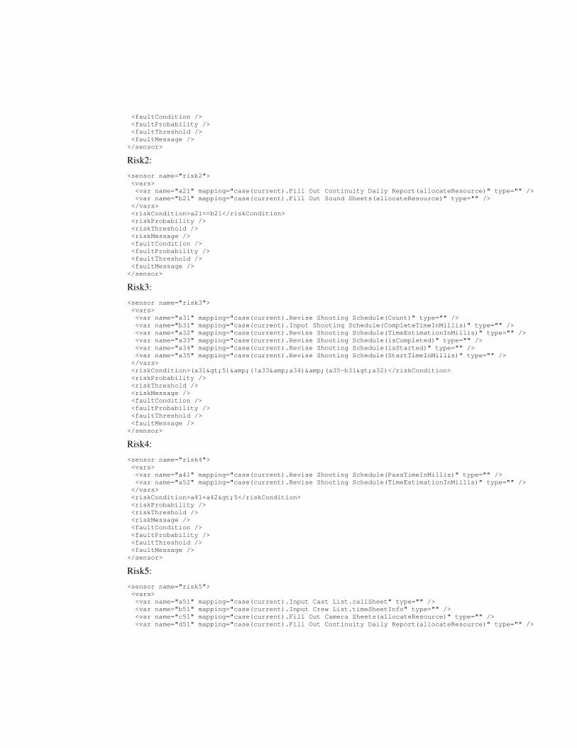
<faultCondition /><faultProbability /><faultThreshold /><faultMessage /></sensor>
Risk2:
<sensor name="risk2"><vars><var name="a21" mapping="case(current).Fill Out Continuity Daily Report(allocateResource)" type="" /><var name="b21" mapping="case(current).Fill Out Sound Sheets(allocateResource)" type="" /></vars><riskCondition>a21==b21</riskCondition><riskProbability /><riskThreshold /><riskMessage /><faultCondition /><faultProbability /><faultThreshold /><faultMessage /></sensor>
Risk3:
<sensor name="risk3"><vars><var name="a31" mapping="case(current).Revise Shooting Schedule(Count)" type="" /><var name="b31" mapping="case(current).Input Shooting Schedule(CompleteTimeInMillis)" type="" /><var name="a32" mapping="case(current).Revise Shooting Schedule(TimeEstimationInMillis)" type="" /><var name="a33" mapping="case(current).Revise Shooting Schedule(isCompleted)" type="" /><var name="a34" mapping="case(current).Revise Shooting Schedule(isStarted)" type="" /><var name="a35" mapping="case(current).Revise Shooting Schedule(StartTimeInMillis)" type="" /></vars><riskCondition>(a31>5)&(!a33&a34)&(a35-b31>a32)</riskCondition><riskProbability /><riskThreshold /><riskMessage /><faultCondition /><faultProbability /><faultThreshold /><faultMessage /></sensor>
Risk4:
<sensor name="risk4"><vars><var name="a41" mapping="case(current).Revise Shooting Schedule(PassTimeInMillis)" type="" /><var name="a52" mapping="case(current).Revise Shooting Schedule(TimeEstimationInMillis)" type="" /></vars><riskCondition>a41+a42>5</riskCondition><riskProbability /><riskThreshold /><riskMessage /><faultCondition /><faultProbability /><faultThreshold /><faultMessage /></sensor>
Risk5:
<sensor name="risk5"><vars><var name="a51" mapping="case(current).Input Cast List.callSheet" type="" /><var name="b51" mapping="case(current).Input Crew List.timeSheetInfo" type="" /><var name="c51" mapping="case(current).Fill Out Camera Sheets(allocateResource)" type="" /><var name="d51" mapping="case(current).Fill Out Continuity Daily Report(allocateResource)" type="" />

</vars><riskCondition>!(a51==b51)&!(c51==d51)</riskCondition><riskProbability /><riskThreshold /><riskMessage /><faultCondition /><faultProbability /><faultThreshold /><faultMessage /></sensor>
Risk6:<sensor name="risk6"><vars><var name="a61" mapping="case(current).Input Crew List.production" type="" /><var name="b61" mapping="case(current).Input Cast List(PassTimeInMillis)" type="" /><var name="c61" mapping="case(current).Input Shooting Schedule(PassTimeInMillis)" type="" /></vars><riskCondition>(a61==5)&((b61+c61)<20)</riskCondition><riskProbability /><riskThreshold /><riskMessage /><faultCondition /><faultProbability /><faultThreshold /><faultMessage /></sensor>
Risk7:<sensor name="risk7"><vars><var name="a71" mapping="case(current).Fill Out Continuity Report.producer" type="" /><var name="b71" mapping="case(current).Fill Out Sound Sheets.production" type="" /><var name="c71" mapping="case(current).Fill Out Camera Sheets.production" type="" /><var name="d71" mapping="case(current).Fill Out AD Report.production" type="" /></vars><riskCondition>!(c71==b71)&(!(b71==a71)|!(b71==d71))</riskCondition><riskProbability /><riskThreshold /><riskMessage /><faultCondition /><faultProbability /><faultThreshold /><faultMessage /></sensor>
B.2 First Experiment: Risks for Process B (Ordering)
Here we list the four risks associated with Process B.Risk2:<sensor name="risk2"><vars><var name="a21" mapping="case(current).Initiate Shipment Status Inquiry(allocateResource)" type="" /><var name="b21" mapping="case(current).Issue Trackpoint Notice(allocateResource)" type="" /></vars><riskCondition>a21==b21</riskCondition><riskProbability /><riskThreshold /><riskMessage /><faultCondition /><faultProbability /><faultThreshold /><faultMessage /></sensor>

Risk4:
<sensor name="risk4"><vars><var name="a41" mapping="case(current).Issue Trackpoint Notice(PassTimeInMillis)" type="" /><var name="a42" mapping="case(current).Issue Trackpoint Notice(TimeEstimationInMillis)" type="" /></vars><riskCondition>a41+a42>5</riskCondition><riskProbability /><riskThreshold /><riskMessage /><faultCondition /><faultProbability /><faultThreshold /><faultMessage /></sensor>
Risk5:
<sensor name="risk5"><vars><var name="a51" mapping="case(current).Issue Trackpoint Notice.AcceptanceCertificate" type="" /><var name="b51" mapping="case(current).Initiate Shipment Status Inquiry.TrackpointNotice" type="" /><var name="c51" mapping="case(current).Log Trackpoint Order Entry(allocateResource)" type="" /><var name="d51" mapping="case(current).Create Acceptance Certificate(allocateResource)" type="" /></vars><riskCondition>!(a51==b51)&!(c51==d51)</riskCondition><riskProbability /><riskThreshold /><riskMessage /><faultCondition /><faultProbability /><faultThreshold /><faultMessage /></sensor>
Risk6:
<sensor name="risk6"><vars><var name="a61" mapping="case(current).Initiate Shipment Status Inquiry.Report" type="" /><var name="b61" mapping="case(current).Issue Trackpoint Notice(PassTimeInMillis)" type="" /><var name="c61" mapping="case(current).Log Trackpoint Order Entry(PassTimeInMillis)" type="" /></vars><riskCondition>(a61==5)&((b61+c61)<20)</riskCondition><riskProbability /><riskThreshold /><riskMessage /><faultCondition /><faultProbability /><faultThreshold /><faultMessage /></sensor>
B.3 First experiment: Risks for Process C (Payment)
Here we list the three risks associated with Process C.
Risk3:
<sensor name="risk3"><vars><var name="a31" mapping="case(current).Approve Purchase Order(Count)" type="" /><var name="b31" mapping="case(current).Create Purchase Order(CompleteTime)" type="" /><var name="a32" mapping="case(current).Approve Purchase Order(TimeEstimationInMillis)" type="" /><var name="a33" mapping="case(current).Approve Purchase Order(isCompleted)" type="" />

<var name="a34" mapping="case(current).Approve Purchase Order(isStarted)" type="" /><var name="a35" mapping="case(current).Approve Purchase Order(StartTimeInMillis)" type="" /></vars><riskCondition>(a31>5)&(!a33&a34)&(a35+b31>a32)</riskCondition><riskProbability /><riskThreshold /><riskMessage /><faultCondition /><faultProbability /><faultThreshold /><faultMessage /></sensor>
Risk4:<sensor name="risk4"><vars><var name="a41" mapping="case(current).Modify Purchase Order(PassTimeInMillis)" type="" /><var name="a42" mapping="case(current).Modify Purchase Order(TimeEstimationInMillis)" type="" /></vars><riskCondition>a41+a42>5</riskCondition><riskProbability /><riskThreshold /><riskMessage /><faultCondition /><faultProbability /><faultThreshold /><faultMessage /></sensor>
Risk6:<sensor name="risk6"><vars><var name="a61" mapping="case(current).Modify Purchase Order.POApproval" type="" /><var name="b61" mapping="case(current).Approve Purchase Order(PassTimeInMillis)" type="" /><var name="c61" mapping="case(current).Confirm Puchase Order(PassTimeInMillis)" type="" /></vars><riskCondition>(a61==5)&((b61+c61)<20)</riskCondition><riskProbability /><riskThreshold /><riskMessage /><faultCondition /><faultProbability /><faultThreshold /><faultMessage /></sensor>
B.4 First experiment: Risks for Process D (Freight in Transit)
Here we list the five risks associated with Process D.
Risk2:<sensor name="risk2"><vars><var name="a21" mapping="case(current).Produce Freight Invoice(allocateResource)" type="" /><var name="b21" mapping="case(current).Issue Shipment Payment Order(allocateResource)" type="" /></vars><riskCondition>a21==b21</riskCondition><riskProbability /><riskThreshold /><riskMessage /><faultCondition /><faultProbability /><faultThreshold /><faultMessage /></sensor>

Risk3:
<sensor name="risk3"><vars><var name="a31" mapping="case(current).Approve Shipment Payment Order(Count)" type="" /><var name="b31" mapping="case(current).Issue Shipment Payment Order(CompleteTime)" type="" /><var name="a32" mapping="case(current).Approve Shipment Payment Order(TimeEstimationInMillis)" type="" /><var name="a33" mapping="case(current).Approve Shipment Payment Order(isCompleted)" type="" /><var name="a34" mapping="case(current).Approve Shipment Payment Order(isStarted)" type="" /><var name="a35" mapping="case(current).Approve Shipment Payment Order(StartTimeInMillis)" type="" /></vars><riskCondition>(a31>5)&(!a33&a34)&(a35+b31>a32)</riskCondition><riskProbability /><riskThreshold /><riskMessage /><faultCondition /><faultProbability /><faultThreshold /><faultMessage /></sensor>
Risk4:
<sensor name="risk4"><vars><var name="a41" mapping="case(current).Approve Shipment Payment Order(PassTimeInMillis)" type="" /><var name="a42" mapping="case(current).Approve Shipment Payment Order(TimeEstimationInMillis)" type="" /></vars><riskCondition>a41+a42>5</riskCondition><riskProbability /><riskThreshold /><riskMessage /><faultCondition /><faultProbability /><faultThreshold /><faultMessage /></sensor>
Risk5:
<sensor name="risk5"><vars><var name="a51" mapping="case(current).Produce Freight Invoice.ShipmentPaymentOrder" type="" /><var name="b51" mapping="case(current).Approve Shipment Payment Order.ShipmentPaymentOrder" type="" /><var name="c51" mapping="case(current).Issue Shipment Invoice(allocateResource)" type="" /><var name="d51" mapping="case(current).Issue Shipment Payment Order(allocateResource)" type="" /></vars><riskCondition>!(a51==b51)&!(c51==d51)</riskCondition><riskProbability /><riskThreshold /><riskMessage /><faultCondition /><faultProbability /><faultThreshold /><faultMessage /></sensor>
Risk6:
<sensor name="risk6"><vars><var name="a61" mapping="case(current).Produce Freight Invoice.ShipmentPaymentOrder" type="" /><var name="b61" mapping="case(current).Issue Shipment Payment Order(PassTimeInMillis)" type="" /><var name="c61" mapping="case(current).Approve Shipment Payment Order(PassTimeInMillis)" type="" /></vars><riskCondition>(a61==5)&((b61+c61)<20)</riskCondition><riskProbability /><riskThreshold />

<riskMessage /><faultCondition /><faultProbability /><faultThreshold /><faultMessage /></sensor>
B.5 Second experiment: Risks Process C (Payment Process)
Here we list the three risks used in the second experiment. These risks are differentfrom the ones used in the first experiment since they use historical information tocompute the risk probability.
Overtime Process risk:
<sensor name="Overtime Process"><vars><var name="d" mapping="5" type="" /><var name="Tc" mapping="case(current).Payment(PassTimeInMillis)" type="" /><var name="Te" mapping="case(current).(TimeEstimationInMillis)" type="" /></vars><riskCondition>(1-(d*24*60*60*1000)/(Te+Tc))>0.6</riskCondition><riskProbability /><riskThreshold /><riskMessage /><faultCondition /><faultProbability /><faultThreshold /><faultMessage /></sensor>
Approval Fraud risk:
<sensor name="Approval Fraud"><vars><var name="sfoA" mapping="case(current).Approve Shipment Payment Order(isAllocated)" type="" /><var name="sfo1" mapping="case(current).Approve Shipment Payment Order(allocateResource)" type="" /><var name="c" mapping="case(current).Issue Shipment Invoice.ShipmentInvoice.Company" type="" /><var name="ASPOa" mapping="case(current).Approve Shipment Payment Order(OfferTimeInMillis)" type="" /><var name="ASPOn" mapping="case(Approve Shipment Payment Order(completeResource)=sfo1 AND
Issue Shipment Invoice.ShipmentInvoice.Company=c ANDApprove Shipment Payment Order(CompleteTimeInMillis)>(ASPOa-(5*24*60*60*1000)) AND(ID)!=[IDCurr]).Approve Shipment Payment Order(CountElements)" type="" />
<var name="sfo2" mapping="case(Issue Shipment Invoice.ShipmentInvoice.Company=c ANDApprove Shipment Payment Order(isCompleted)="true"AND Approve Shipment Payment Order(CompleteTimeInMillis)>(ASPOa-(5*24*60*60*1000))AND (ID)!=[IDCurr]).Approve Shipment Payment Order(completeResource)" type="" />
<var name="sfo" mapping="case(current).Approve Shipment Payment Order(offerDistribution)" type="" /></vars><riskCondition>(ASPOn>0)|(!sfoA&(sfo2.startedMinNumber==0)&(sfo.startedMinNumberExcept.sfo2>=1))</riskCondition><riskProbability /><riskThreshold /><riskMessage /><faultCondition /><faultProbability /><faultThreshold /><faultMessage /></sensor>
Order Unfulfillment risk:
<sensor name="Order Unfulfillment"><vars>

<var name="USPOuc" mapping="case(current).Update Shipment Payment Order(Count)" type="" /><var name="USPOu5" mapping="case(Update Shipment Payment Order(Count)>=5).
Update Shipment Payment Order(CountElements)" type="" /><var name="USPOus" mapping="case(Update Shipment Payment Order(Count)>=USPOuc AND
Process Shipment Payment(isOffered)="true").Update Shipment Payment Order(CountElements)" type="" />
</vars><riskCondition>(USPOu5/USPOus)>0.7</riskCondition><riskProbability /><riskThreshold /><riskMessage /><faultCondition /><faultProbability /><faultThreshold /><faultMessage /></sensor>
C Solutions second experiment
Here we list the solutions proposed for the second experiment.
Model: - Time: 60009 -
Solution1risk1 0.0, prob1 0.0, risk2 0.0, prob2 0.0, risk3 0.0, prob3 0.0, cost 50.0RemoveAllocateRes: Approve Shipment Payment Order <participant id="PA-223a865e-9b16-4c0b-a496-4e445eaad1ec">RemoveOfferRes: Approve Shipment Payment Order <participant id="PA-0b7f1d4c-f3b2-4fd4-8e77-c33f65bb2821">RemoveOfferRes: Approve Shipment Payment Order <participant id="PA-223a865e-9b16-4c0b-a496-4e445eaad1ec">RemoveOfferRes: Approve Shipment Payment Order <participant id="PA-3dad7d51-ffbd-4e02-aeba-462deac95ef8">Rollback: Update Shipment Payment OrderRollback: Approve Shipment Payment OrderTauize: Issue Shipment Remittance AdviceRollback: Update Shipment Payment OrderTauize: Approve Shipment Payment Order
Solution2risk1 0.0, prob1 0.0, risk2 0.0, prob2 0.0, risk3 0.0, prob3 0.0, cost 50.0RemoveAllocateRes: Approve Shipment Payment Order <participant id="PA-223a865e-9b16-4c0b-a496-4e445eaad1ec">RemoveOfferRes: Approve Shipment Payment Order <participant id="PA-0b7f1d4c-f3b2-4fd4-8e77-c33f65bb2821">RemoveOfferRes: Approve Shipment Payment Order <participant id="PA-223a865e-9b16-4c0b-a496-4e445eaad1ec">RemoveOfferRes: Approve Shipment Payment Order <participant id="PA-3dad7d51-ffbd-4e02-aeba-462deac95ef8">Rollback: Update Shipment Payment OrderRollback: Approve Shipment Payment OrderTauize: Issue Shipment Remittance AdviceRollback: Update Shipment Payment OrderTauize: Issue Debit Adjustment
Solution3risk1 0.0, prob1 0.0, risk2 0.0, prob2 0.0, risk3 25.0, prob3 0.0, cost 41.0RemoveAllocateRes: Approve Shipment Payment Order <participant id="PA-223a865e-9b16-4c0b-a496-4e445eaad1ec">RemoveOfferRes: Approve Shipment Payment Order <participant id="PA-0b7f1d4c-f3b2-4fd4-8e77-c33f65bb2821">RemoveOfferRes: Approve Shipment Payment Order <participant id="PA-223a865e-9b16-4c0b-a496-4e445eaad1ec">RemoveOfferRes: Approve Shipment Payment Order <participant id="PA-3dad7d51-ffbd-4e02-aeba-462deac95ef8">Rollback: Update Shipment Payment OrderRollback: Approve Shipment Payment OrderTauize: Update Shipment Payment OrderTauize: Process Shipment Payment
Solution4risk1 0.0, prob1 0.0, risk2 0.0, prob2 0.0, risk3 25.0, prob3 0.0, cost 41.0RemoveAllocateRes: Approve Shipment Payment Order <participant id="PA-223a865e-9b16-4c0b-a496-4e445eaad1ec">RemoveOfferRes: Approve Shipment Payment Order <participant id="PA-0b7f1d4c-f3b2-4fd4-8e77-c33f65bb2821">RemoveOfferRes: Approve Shipment Payment Order <participant id="PA-223a865e-9b16-4c0b-a496-4e445eaad1ec">RemoveOfferRes: Approve Shipment Payment Order <participant id="PA-3dad7d51-ffbd-4e02-aeba-462deac95ef8">Rollback: Update Shipment Payment Order

Rollback: Approve Shipment Payment OrderTauize: Update Shipment Payment OrderTauize: Approve Shipment Payment Order
Solution5risk1 0.0, prob1 0.0, risk2 0.0, prob2 0.0, risk3 75.0, prob3 0.0, cost 19.0RemoveAllocateRes: Approve Shipment Payment Order <participant id="PA-223a865e-9b16-4c0b-a496-4e445eaad1ec">Tauize: Issue Shipment Remittance AdviceTauize: Process Shipment PaymentRestoreAllocateRes: Approve Shipment Payment Order <participant id="PA-3dad7d51-ffbd-4e02-aeba-462deac95ef8">
Solution6risk1 0.0, prob1 0.0, risk2 0.0, prob2 0.0, risk3 75.0, prob3 0.0, cost 19.0RemoveAllocateRes: Approve Shipment Payment Order <participant id="PA-223a865e-9b16-4c0b-a496-4e445eaad1ec">RestoreAllocateRes: Approve Shipment Payment Order <participant id="PA-0b7f1d4c-f3b2-4fd4-8e77-c33f65bb2821">Tauize: Issue Debit AdjustmentTauize: Issue Shipment Remittance Advice
Solution7risk1 75.0, prob1 0.0, risk2 0.0, prob2 0.0, risk3 00.0, prob3 0.0, cost 41.0RemoveAllocateRes: Approve Shipment Payment Order <participant id="PA-223a865e-9b16-4c0b-a496-4e445eaad1ec">RemoveOfferRes: Approve Shipment Payment Order <participant id="PA-0b7f1d4c-f3b2-4fd4-8e77-c33f65bb2821">RemoveOfferRes: Approve Shipment Payment Order <participant id="PA-223a865e-9b16-4c0b-a496-4e445eaad1ec">RemoveOfferRes: Approve Shipment Payment Order <participant id="PA-3dad7d51-ffbd-4e02-aeba-462deac95ef8">Rollback: Update Shipment Payment OrderRollback: Approve Shipment Payment OrderTauize: Issue Shipment Remittance AdviceRollback: Update Shipment Payment Order
Solution8risk1 75.0, prob1 0.0, risk2 0.0, prob2 0.0, risk3 25.0, prob3 0.0, cost 32.0RemoveAllocateRes: Approve Shipment Payment Order <participant id="PA-223a865e-9b16-4c0b-a496-4e445eaad1ec">RemoveOfferRes: Approve Shipment Payment Order <participant id="PA-0b7f1d4c-f3b2-4fd4-8e77-c33f65bb2821">RemoveOfferRes: Approve Shipment Payment Order <participant id="PA-223a865e-9b16-4c0b-a496-4e445eaad1ec">RemoveOfferRes: Approve Shipment Payment Order <participant id="PA-3dad7d51-ffbd-4e02-aeba-462deac95ef8">Rollback: Update Shipment Payment OrderRollback: Approve Shipment Payment OrderTauize: Update Shipment Payment Order
Solution9risk1 75.0, prob1 0.0, risk2 0.0, prob2 0.0, risk3 75.0, prob3 0.0, cost 1.0RemoveAllocateRes: Approve Shipment Payment Order <participant id="PA-223a865e-9b16-4c0b-a496-4e445eaad1ec">RestoreAllocateRes: Approve Shipment Payment Order <participant id="PA-0b7f1d4c-f3b2-4fd4-8e77-c33f65bb2821">
Solution10risk1 0.0, prob1 0.0, risk2 75.0, prob2 0.0, risk3 75.0, prob3 0.0, cost 18.0Tauize: Process Shipment PaymentTauize: Issue Shipment Remittance Advice
total model generated: 1015