automated remote cameras for monitoring alluvial … · · 2018-02-27automated remote cameras for...
TRANSCRIPT

U.S. Department of the Interior U.S. Geological Survey
Prepared in cooperation with Northern Arizona University
Automated Remote Cameras for Monitoring Alluvial Sandbars on the Colorado River in Grand Canyon, Arizona
By Paul E. Grams, Robert B. Tusso, and Daniel Buscombe
Open-File Report 2018–1019

ii
Cover image: Photograph of sandbar that is photographed daily by remote digital camera (in foreground) along the Colorado River in Grand Canyon National Park, Arizona.

U.S. Department of the Interior U.S. Geological Survey
Prepared in cooperation with Northern Arizona University
Automated Remote Cameras for Monitoring Alluvial Sandbars on the Colorado River in Grand Canyon, Arizona
By Paul E. Grams, Robert B. Tusso, and Daniel Buscombe
Open-File Report 2018–1019

iv
U.S. Department of the Interior RYAN K. ZINKE, Secretary
U.S. Geological Survey William H. Werkheiser, Deputy Director
exercising the authority of the Director
U.S. Geological Survey, Reston, Virginia: 2018
For more information on the USGS—the Federal source for science about the Earth, its natural and living resources, natural hazards, and the environment—visit https://www.usgs.gov/ or call 1–888–ASK–USGS (1–888–275–8747).
For an overview of USGS information products, including maps, imagery, and publications, visit https://store.usgs.gov/.
Any use of trade, firm, or product names is for descriptive purposes only and does not imply endorsement by the U.S. Government.
Although this information product, for the most part, is in the public domain, it also may contain copyrighted materials as noted in the text. Permission to reproduce copyrighted items must be secured from the copyright owner.
Suggested citation: Grams, P.E., Tusso, R.B., and Buscombe, D., 2018, Automated remote cameras for monitoring alluvial sandbars on the Colorado River in Grand Canyon, Arizona: U.S. Geological Survey Open-File Report 2018–1019, 50 p., https://doi.org/10.3133/ofr20181019.
ISSN 2331-1258 (online)

v
Acknowledgments
We thank the many individuals who have contributed to the development, construction, and maintenance of the remote camera systems described in this report. Glen Bennett and Ted Melis initiated the transition from film to the new digital cameras in 2008 and the original 12 cameras (most of which are still in service) were built by Rian Bogle. Tim Dealy assisted with building many of the cameras currently in use. Many cooperators and volunteers have assisted with servicing the cameras and exchanging memory cards in the field including Matt Kaplinski, Ryan Lima, Tom Sabol, Ron Griffiths, and Joel Unema. Joseph Hazel, Keith Kohl, Rob Ross, and Rod Parnell surveyed the locations of cameras and panels used for image rectification. Julaire Scott and Caleb Ring assisted with organizing the thousands of scanned images from the original film cameras. Finally, Tom Gushue, Tim Andrews, Taylor Johnson, and James Hensleigh, developed the tools to display and serve the images online. This work was supported by the Glen Canyon Dam Adaptive Management Program and the U.S. Department of Interior Bureau of Reclamation.

vi
Contents Acknowledgments .......................................................................................................................................................... v
Abstract .......................................................................................................................................................................... 1
Introduction .................................................................................................................................................................... 1
Study Area and Monitoring Locations ............................................................................................................................ 2
Description of Remote-Camera Systems ....................................................................................................................... 6
Film-Camera Systems ................................................................................................................................................ 6
Digital-Camera Systems ............................................................................................................................................. 7
Image Processing and Analysis ..................................................................................................................................... 9
Image Processing and Web-Based Image Viewer ..................................................................................................... 9
Qualitative Analysis of Sandbar Deposition and Erosion ......................................................................................... 11
Method Validation ................................................................................................................................................ 14
Results of Visual Estimates of Sandbar Change ................................................................................................. 17
Quantitative Analysis of Sandbar Area ..................................................................................................................... 19
Image Registration and Rectification ................................................................................................................... 19
Delineation of Sandbar Area ............................................................................................................................... 23
The RCSandSeg Program ................................................................................................................................... 25
Sandbar Area at RC0307 Between October 2009 and October 2015 ......................................................................... 30
References Cited ......................................................................................................................................................... 37
Appendix 1. Normalized Changes in Sandbar Area, Volume, and Composite Sandbar Size on the Colorado River in Grand Canyon National Park, Arizona, Determined from Repeat Topographic Surveys ...................................... 40
Appendix 2. Estimated Changes in sandbar size on the Colorado River in Grand Canyon National Park, Arizona, from Remote-Camera Images for the 2012, 2013, 2014, and 2016 Controlled Floods Released from Glen Canyon Dam ......................................................................................................................................................... 41
Appendix 3. Example Python Computer Program for Finding the [x,y] Translation Vector Between Two Remote-Camera Images Used for Monitoring Sandbars on the Colorado River in Grand Canyon National Park, Arizona, Using Two-dimensional Fast Fourier Transform (2D-FFT) ................................................................................... 49
Appendix 4. Example Python Computer Program for Finding the Area of a Polygon in Projected [x,y] Coordinates .. 50

vii
Figures Figure 1. Map of Colorado River corridor in Glen Canyon National Recreation Area and Grand Canyon
National Park, Arizona, showing the locations of sandbar monitoring sites with remote cameras ................. 3
Figure 2. Photograph of debris fan and downstream eddy showing typical alluvial sandbar formations
along the Colorado River in Grand Canyon National Park, Arizona. .............................................................. 4
Figure 3. Photographs of remote-camera systems used along the Colorado River in Grand Canyon
National Park, Arizona ................................................................................................................................... 7
Figure 4. Graph of discharge of the Colorado River at Lees Ferry, Arizona ......................................... 12
Figure 5. Photographs of sandbars along the Colorado River in Grand Canyon National Park, Arizona,
from before and after the 2014 controlled flood released from Glen Canyon Dam ...................................... 13
Figure 6. Graphs of visual estimates of change in sandbar size in remote-camera images from
monitoring sites along the Colorado River in Grand Canyon National Park, Arizona, following controlled
floods released from Glen Canyon Dam ...................................................................................................... 19
Figure 7. Example of the image-registration workflow used for sandbar monitoring along the Colorado
River in Grand Canyon National Park, Arizona ............................................................................................ 20
Figure 8. Example of the image rectification workflow used for sandbar monitoring along the Colorado
River in Grand Canyon National Park, Arizona ............................................................................................ 21
Figure 9. Example oblique photograph taken by a remote camera used for sandbar monitoring along
the Colorado River in Grand Canyon National Park, Arizona ...................................................................... 23
Figure 10. Time series of oblique imagery from a sandbar monitoring site (RC0307R) along the
Colorado River in Grand Canyon National Park, Arizona ............................................................................ 24
Figure 11. Screenshots from the RCSandSeg program used to process remote-camera images for
sandbar monitoring along the Colorado River in Grand Canyon National Park, Arizona ............................. 26

viii
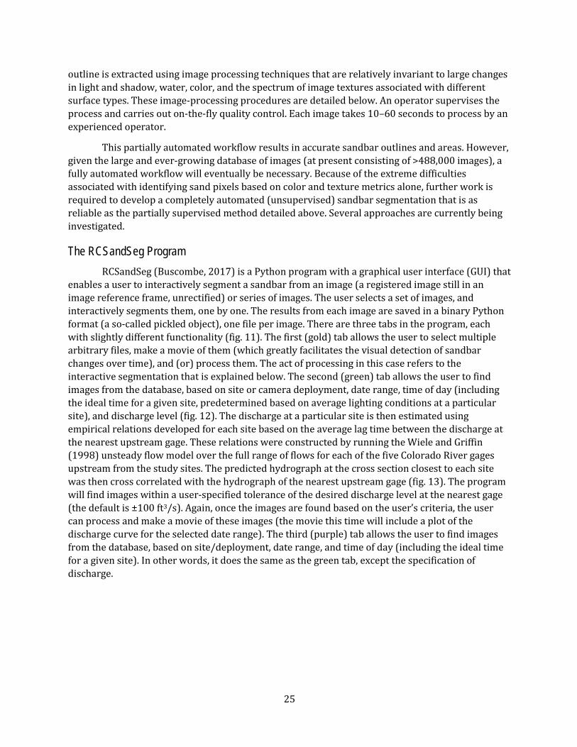
Figure 12. Screenshots from the green tab of the RCSandSeg program used to process remote-camera
images for sandbar monitoring along the Colorado River in Grand Canyon National Park, Arizona ........... 27
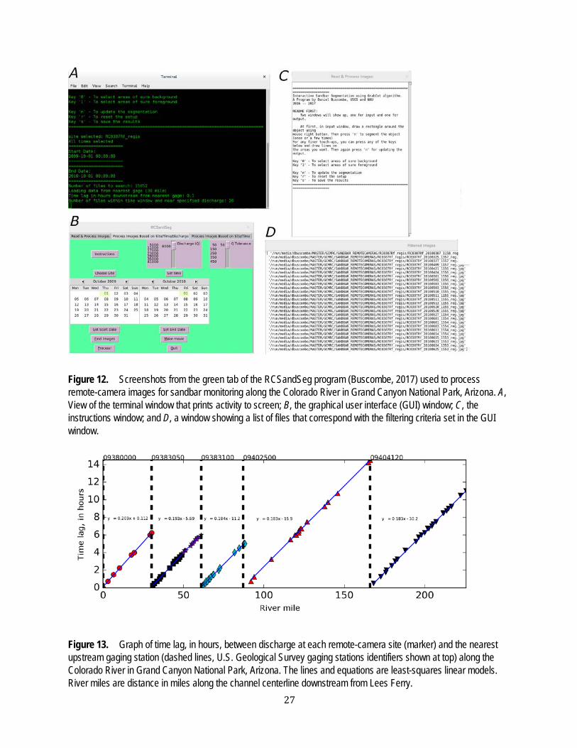
Figure 13. Graph of time lag, in hours, between discharge at each remote-camera site and the nearest
upstream gaging station along the Colorado River in Grand Canyon National Park, Arizona...................... 27
Figure 14. Example interactive segmentation in the RCSandSeg program (Buscombe, 2017) used to
process remote-camera images for sandbar monitoring along the Colorado River in Grand Canyon National
Park, Arizona. .............................................................................................................................................. 29
Figure 15. Time series of oblique remote-camera imagery..................................................................... 33
Figure 16. Graph of the relation between survey-derived and image-derived sandbar area above the
river stage associated with a flow rate of 10,000 cubic feet per second along the Colorado River in Grand
Canyon National Park, Arizona .................................................................................................................... 34
Figure 17. Graphs showing time series since 1990 of total-station survey-derived and image-derived
sandbar areas above the river stage associated with a flow rate of 10,000 cubic feet per second along the
Colorado River in Grand Canyon National Park, Arizona ............................................................................ 35
Figure 18. Images showing comparisons between rectified sandbars used for sandbar monitoring along
the Colorado River in Grand Canyon National Park .................................................................................... 36
Tables Table 1. Sandbar monitoring sites with remote camera systems along the Colorado River in Grand
Canyon National Park, Arizona ...................................................................................................................... 5
Table 2. Digital-camera models used in remote camera systems along the Colorado River in Grand
Canyon National Park, Arizona. ..................................................................................................................... 8
Table 3. Periods of image record at sandbar monitoring sites where camera locations have changed
along the Colorado River in Grand Canyon National Park, Arizona. ............................................................ 10

ix
Table 4. Visually estimated changes in sandbar size in remote-camera images taken along the
Colorado River in Grand Canyon National Park, Arizona ............................................................................ 14
Table 5. Comparison between visual estimates of sandbar change in remote-camera images and
measured sandbar change at monitoring sites ............................................................................................ 16
Table 6. Matrix of agreement and disagreement between measured change in normalized sandbar
size and visually estimated change in sandbar size in remote camera images at monitoring sites along the
Colorado River in Grand Canyon National Park, Arizona. ........................................................................... 17
x
Conversion Factors U.S. customary units to International System of Units
Multiply By To obtain
Length
inch (in.) 2.54 centimeter (cm)
foot (ft) 0.3048 meter (m)
mile (mi) 1.609 kilometer (km)
Area
square foot (ft2) 0.09290 square meter (m2)
Flow Rate
cubic foot per second (ft3/s) 0.02832 cubic meter per second (m3/s)
International System of Units to U.S. customary units
Multiply By To obtain
Length
centimeter (cm) 0.3937 inch (in.)
meter (m) 3.281 foot (ft)
kilometer (km) 0.6214 mile (mi)
Area
square meter (m2) 10.76 square foot (ft2)
Flow rate
cubic meter per second (m3/s) 35.31 cubic foot per second (ft3/s)
Datum Vertical coordinate information is referenced to the Geodetic Reference System 1980 (GRS 80) ellipse defined by the North American Datum of 1983 (NAD 83) (2011). Horizontal coordinate information is referenced to NAD 83 (2011) and projected to State Plane Coordinate System, Arizona Central Zone, in meters. Elevation, as used in this report, refers to distance above the Geodetic Reference System 1980 (GRS 80) ellipse defined by the North American Datum of 1983 (NAD 83) (2011).

xi
Abbreviations 2D-FFT two-dimensional fast Fourier transform DC direct current Exif exchangeable image file format GCMRC Grand Canyon Monitoring and Research Center GCP ground control point GUI graphical user interface ft3/s cubic feet per second RANSAC random sample consensus RM river mile RMSE root-mean-square error RCSandSeg Remote Camera Sandbar Segmentation computer program SIFT scale invariant feature transform USGS U.S. Geological Survey
1
Automated Remote Cameras for Monitoring Alluvial Sandbars on the Colorado River in Grand Canyon, Arizona
By Paul E. Grams1, Robert B. Tusso1, and Daniel Buscombe2
Abstract Automated camera systems deployed at 43 remote locations along the Colorado River
corridor in Grand Canyon National Park, Arizona, are used to document sandbar erosion and deposition that are associated with the operations of Glen Canyon Dam. The camera systems, which can operate independently for a year or more, consist of a digital camera triggered by a separate data controller, both of which are powered by an external battery and solar panel. Analysis of images for categorical changes in sandbar size show deposition at 50 percent or more of monitoring sites during controlled flood releases done in 2012, 2013, 2014, and 2016. The images also depict erosion of sandbars and show that erosion rates were highest in the first 3 months following each controlled flood. Erosion rates were highest in 2015, the year of highest annual dam release volume. Comparison of the categorical estimates of sandbar change agree with sandbar change (erosion or deposition) measured by topographic surveys in 76 percent of cases evaluated. A semiautomated method for quantifying changes in sandbar area from the remote-camera images by rectifying the oblique images and segmenting the sandbar from the rest of the image is presented. Calculation of sandbar area by this method agrees with sandbar area determined by topographic survey within approximately 8 percent and allows quantification of sandbar area monthly (or more frequently).
Introduction Sandbars that occur along the banks of the Colorado River in Grand Canyon National Park
and Glen Canyon National Recreation Area, Arizona, have long been recognized as integral components of the riverine landscape and an important resource. Sandbars serve as the primary boat landing and camping sites for the thousands of overnight visitors to the river corridor each year (Stewart and others, 2003). Sandy alluvium provides substrate for riparian vegetation, which forms the terrestrial riparian ecosystem (Ralston, 2005). The morphological characteristics of some sandbars create streambank irregularities that are low-velocity habitat for native fish (Valdez and Ryel, 1995; Converse and others, 1998). The bare sand exposed on sandbars is also a source of windblown sand for upland aeolian dune fields that contain historical and archeological sites (East
1U.S. Geological Survey.
2Northern Arizona University.
2
and others, 2016). For all of these reasons, sandbars and changes in sandbar size and character are of interest to resource managers and the public.
Scientific investigations have described sandbar characteristics (Schmidt, 1990), mechanisms of sandbar erosion (Budhu and Gobin, 1995; Alvarez and Schmeeckle, 2013), and rates and magnitudes of deposition (Hazel and others, 1999, 2010; Schmidt and others, 1999). Sandbars have eroded, decreasing in size and number since the completion of Glen Canyon Dam in 1963 (Dolan and others, 1974; Schmidt and Graf, 1990; Schmidt and others, 2004; Ross and Grams, 2015). Schmidt and others (2004) estimated the extent of exposed sand decreased by approximately 25 percent. Erosion was associated with a corresponding decrease in campsites available to river recreationists (Kearsley and others, 1994). In 1996, the U.S. Department of the Interior began experiments with controlled flood releases from Glen Canyon Dam to rebuild eroded sandbars (Webb and others, 1999). That initial experiment and subsequent experimental releases in 2004 and 2008 demonstrated that controlled floods under the appropriate conditions of sediment supply were an effective tool for rebuilding eroded sandbars (Schmidt and Grams, 2011). Building on these findings, the U.S. Department of the Interior adopted a protocol for releasing controlled floods annually, depending on resource conditions (Wright and Kennedy, 2011; U.S. Department of the Interior, 2012). Preliminary findings indicate continued effectiveness of this approach (Grams and others, 2015).
Assessment of sandbar condition and response to the controlled floods of 1996, 2004, and 2008 has been based primarily on annual (or more frequent) topographic surveys of a collection of long-term monitoring sites (Hazel and others, 2010). These surveys consist of measurements of sandbar topography above the elevation associated with a discharge of 8,000 cubic feet per second (ft3/s). The topographic maps derived from these surveys are used to calculate sandbar area and sandbar volume for each site. Although these surveys are accurate and reliable, data collection requires a 16-day river expedition with a crew of 12 or more scientists, technicians, and boat operators (Hazel and others, 2010). Processing and analysis of the data requires an additional 8 to 12 weeks of office time for one or two scientists. Although the accuracy and level of detail provided by the surveys was essential for documenting the effects of the initial controlled floods (Hazel and others, 1999; Hazel and others, 2010; Schmidt and Grams, 2011), conducting preflood and postflood release survey expeditions for every subsequent controlled flood is prohibitively time consuming and expensive. As an alternative, the U.S. Geological Survey (USGS) Grand Canyon Monitoring and Research Center (GCMRC) in partnership with Northern Arizona University established a network of remotely deployed digital cameras to collect daily images of selected monitoring sites. These cameras are used to document the depositional (or erosional) response of controlled floods and to document changes to sandbars that occur following controlled floods. This report describes the remote camera systems, the locations where those cameras are maintained, analyses performed on the images to document sandbar changes, and image-based assessment of controlled floods conducted in 2012, 2013, 2014, and 2016.
Study Area and Monitoring Locations The sandbar-monitoring sites discussed in this report are along the Colorado River corridor
within Grand Canyon National Park. Locations are referenced by the GCMRC river mile (RM) system, which is distance in miles along the channel centerline downstream from Lees Ferry, Arizona. Lees Ferry (RM 0) is located 15.5 miles (mi) (21.4 kilometers, km) downstream from Glen Canyon Dam,
3
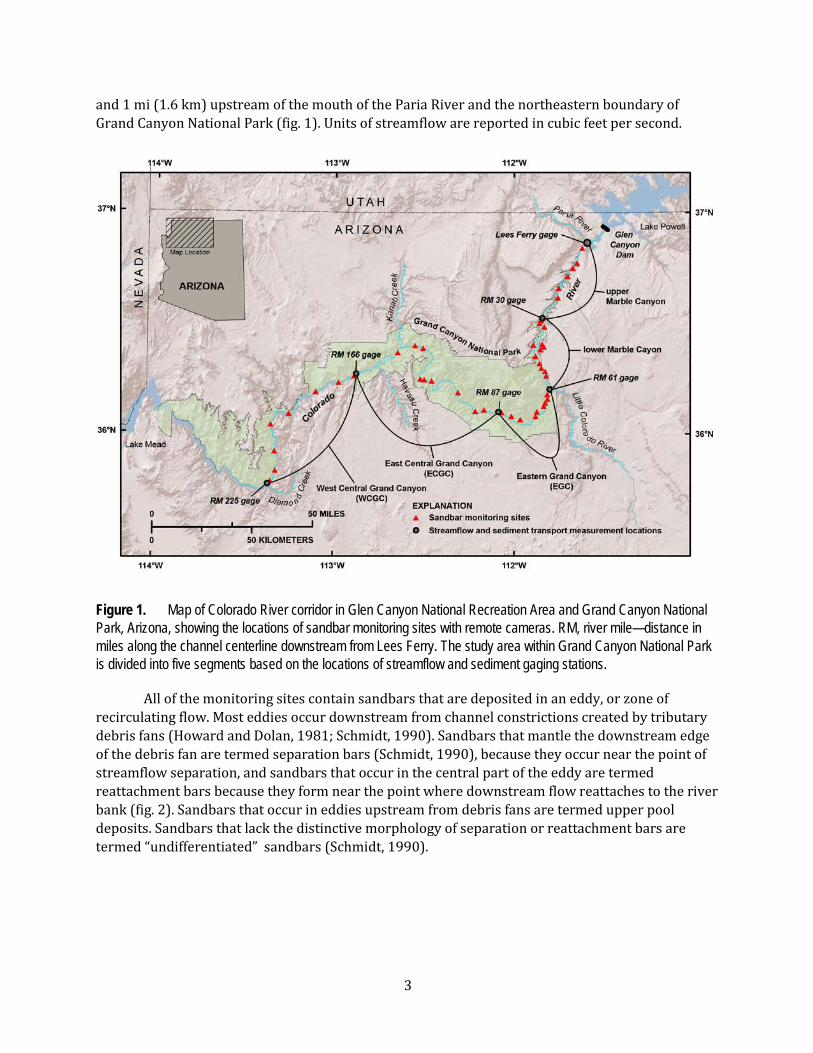
and 1 mi (1.6 km) upstream of the mouth of the Paria River and the northeastern boundary of Grand Canyon National Park (fig. 1). Units of streamflow are reported in cubic feet per second.
Figure 1. Map of Colorado River corridor in Glen Canyon National Recreation Area and Grand Canyon National Park, Arizona, showing the locations of sandbar monitoring sites with remote cameras. RM, river mile—distance in miles along the channel centerline downstream from Lees Ferry. The study area within Grand Canyon National Park is divided into five segments based on the locations of streamflow and sediment gaging stations.
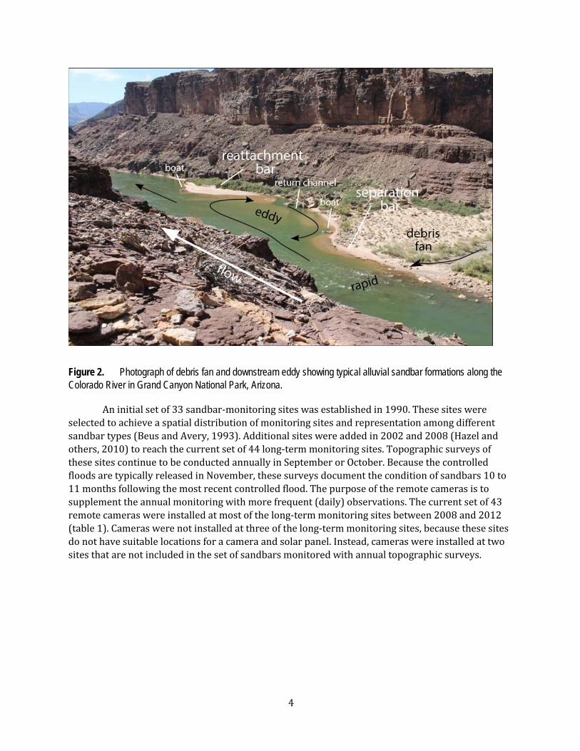
All of the monitoring sites contain sandbars that are deposited in an eddy, or zone of recirculating flow. Most eddies occur downstream from channel constrictions created by tributary debris fans (Howard and Dolan, 1981; Schmidt, 1990). Sandbars that mantle the downstream edge of the debris fan are termed separation bars (Schmidt, 1990), because they occur near the point of streamflow separation, and sandbars that occur in the central part of the eddy are termed reattachment bars because they form near the point where downstream flow reattaches to the river bank (fig. 2). Sandbars that occur in eddies upstream from debris fans are termed upper pool deposits. Sandbars that lack the distinctive morphology of separation or reattachment bars are termed “undifferentiated” sandbars (Schmidt, 1990).
4
Figure 2. Photograph of debris fan and downstream eddy showing typical alluvial sandbar formations along the Colorado River in Grand Canyon National Park, Arizona.
An initial set of 33 sandbar-monitoring sites was established in 1990. These sites were selected to achieve a spatial distribution of monitoring sites and representation among different sandbar types (Beus and Avery, 1993). Additional sites were added in 2002 and 2008 (Hazel and others, 2010) to reach the current set of 44 long-term monitoring sites. Topographic surveys of these sites continue to be conducted annually in September or October. Because the controlled floods are typically released in November, these surveys document the condition of sandbars 10 to 11 months following the most recent controlled flood. The purpose of the remote cameras is to supplement the annual monitoring with more frequent (daily) observations. The current set of 43 remote cameras were installed at most of the long-term monitoring sites between 2008 and 2012 (table 1). Cameras were not installed at three of the long-term monitoring sites, because these sites do not have suitable locations for a camera and solar panel. Instead, cameras were installed at two sites that are not included in the set of sandbars monitored with annual topographic surveys.

5
Table 1. Sandbar monitoring sites with remote camera systems along the Colorado River in Grand Canyon National Park, Arizona, with periods of film records, digital-image records, and topographic surveys.
[L, left; R, right; NA, not applicable]
Site ID Site name River mile
River side
Number of camera
locations
Begin film record
End film record
Begin digital record
Topographic surveys
0025L Cathedral Wash 2.5 L 1 Mar 1992 Feb 2010 Feb 2010 1990–present
0081L Jackass Camp 8.1 L 2 Mar 1992 Feb 2010 Feb 2012 1990–present
0089L 9-Mile 8.9 L 1 NA Oct 2012 Oct 2012 2008–present
0166L Hot Na Na Wash 16.6 L 1 Mar 1992 Nov 2004 Nov 2004 1990–present
0220R 22-Mile 22.0 R 3 Feb 1996 Oct 2004 Feb 2010 1990–present
0235L Lone Cedar 23.5 L 1 NA NA Feb 2013 2002–present
0295L Silver Grotto 29.5 L 0 NA NA NA 1990–present
0307R Sand Pile 30.7 R 6 NA NA Aug 2008 1990–present
0319R South Canyon 31.9 R 1 NA NA Feb 2012 1990–present
0333L Redwall Cavern 33.3 L 1 NA NA Oct 2013 1990–present
0351L Nautiloid Canyon
35.1 L 0 NA NA NA 1990–present
0414R Buck Farm 41.4 R 1 Sep 2002 Feb 2010 Feb 2010 1990–present
0434L Anasazi Bridge 43.4 L 1 Mar 1992 Apr 1994 Oct 2012 1990–present
0445L Eminence 44.5 L 1 Mar 1993 Feb 2010 July 2008 1990–present
0450L Willie Taylor 45.0 L 1 NA NA Feb 2008 2002–present
0476R Saddle 47.6 R 2 NA NA Feb 2011 1990–present
0501R Dinosaur 50.1 R 1 Jan 1996 Oct 2011 Oct 2011 1990–present
0515L 51-Mile 51.5 L 1 NA NA Feb 2008 1990–present
0559R Kwagunt Marsh 55.9 R 1 Feb 1996 Feb 2010 Feb 2010 1991–present
0566R Kwagunt Beach 56.6 R 1 NA NA Oct 2012 2002–present
0629R Crash Canyon 62.9 R 1 NA NA Feb 2013 1993–present
0651R Carbon 65.1 R 1 NA NA Oct 2012 1996–present
0658L Above Lava-Chuar
65.8 L 1 NA NA Feb 2008 2008 only
0661L Palisades 66.1 L 4 NA NA Feb 2011 2008 only
0688R Tanner Rapid 68.7 R 1 Dec 1990 Oct 2011 Oct 2011 1990–present
0701R Lower Basalt 70.1 R 1 Feb 2008 standby April 2013 2008–present

6
Site ID Site name River mile
River side
Number of camera
locations
Begin film record
End film record
Begin digital record
Topographic surveys
0817L Grapevine 81.7 L 1 Apr 1992 Feb 2010 Feb 2010 1990–present
0846R Clear Creek 84.6 R 1 NA NA Oct 2013 2002–present
0876L Upper Cremation 87.7 L 1 Jan 1996 Aug 2012 NA 1990–present
0917R Above Trinity Camp
91.7 R 1 Jan 1996 Oct 2012 Oct 2012 1990–present
0938L Granite 93.8 L 1 NA NA Feb 2012 1990–present
1044R Emerald 104.5 R 1 Jan 1996 Oct 2012 Oct 2012 1990–present
1194R Big Dune 119.4 R 1 Mar 1992 Feb 2010 Feb 2010 1990–present
1227R 122-Mile 122.8 R 1 Mar 1992 Feb 2011 Feb 2011 1990–present
1233L Upper Forster 123.3 L 3 NA NA Oct 2013 1990–present
1377L Football Field 137.7 L 1 Apr 1992 Feb 2010 Feb 2010 1990–present
1396R Fishtail 139.6 R 1 Jan 1996 Feb 2010 NA 1990–present
1459L Above Olo 145.9 L 1 Mar 1992 Feb 2010 Feb 2010 1990–present
1671L Lower National 167.1 L 1 NA NA Feb 2013 2002–present
1726L Below Mohawk 172.6 L 2 NA NA Feb 2010 1990–present
1833R Below Chevron 183.3 R 1 Mar 1992 Feb 2011 Feb 2011 1990–present
1946L Hualapai Acres 194.6 L 1 Jan 1996 Feb 2010 Feb 2010 1990–present
2023R 202-Mile 202.3 R 1 Jan 1996 Feb 2010 Feb 2010 1990–present
2133L Pumpkin Springs 213.3 L 1 Jan 1996 Oct 2013 Oct 2013 1990–present
2201R Middle 220-Mile 220.1 R 1 NA NA Oct 2013 1990–present
2255R Above Last Chance
225.5 R 2 Feb 2010 Feb 2010 Feb 2010 1990–present
Description of Remote-Camera Systems
Film-Camera Systems Although the primary purpose of this report is to describe the digital-camera systems that
are currently in use, daily images were collected periodically at many of the same sites between 1990 and 2008 with film cameras (Cluer, 1995). These systems consisted of a film camera with integrated intervalometer mounted in a weatherproof enclosure (fig. 3). All film systems used a Pentax IQZ 105 camera and either 24 or 36 exposure diapositive (slide) film. These cameras only allowed use of single, fixed intervals with a maximum interval of 1 day, which was used for all deployments. The time of day the image was taken was determined by the time of day the camera
7
was visited and set to trigger. At each visit, camera batteries were replaced, old film was retrieved, new film loaded, and the interval triggered. The number of images (and number of days of images) was limited to the number of exposures available. Occasionally, field visits were scheduled to maintain the cameras, but for most sites there are many gaps in the record of images for the 1990 to 2008 period, which represent lapses between field visits. Table 1 lists the periods during which film cameras were present at each site; however, images are not available continuously for the period of record.
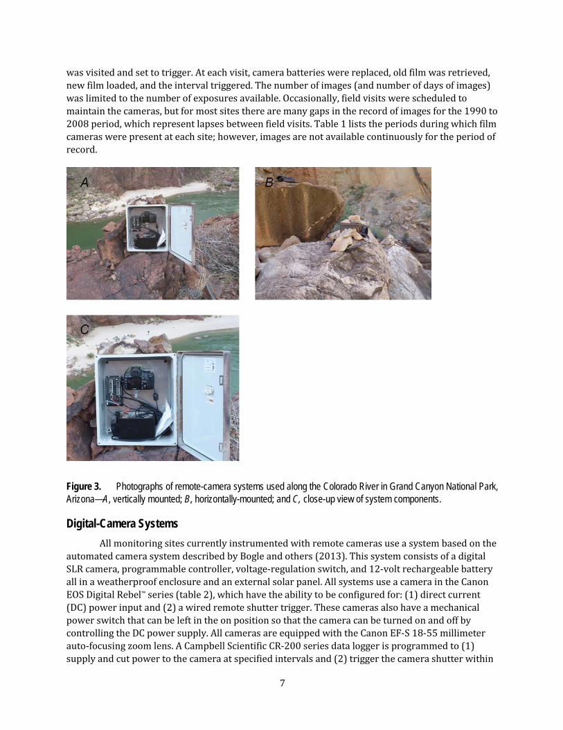
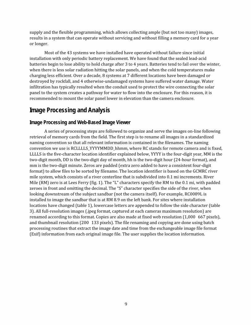
Figure 3. Photographs of remote-camera systems used along the Colorado River in Grand Canyon National Park, Arizona—A, vertically mounted; B, horizontally-mounted; and C, close-up view of system components.
Digital-Camera Systems All monitoring sites currently instrumented with remote cameras use a system based on the
automated camera system described by Bogle and others (2013). This system consists of a digital SLR camera, programmable controller, voltage-regulation switch, and 12-volt rechargeable battery all in a weatherproof enclosure and an external solar panel. All systems use a camera in the Canon EOS Digital Rebel™ series (table 2), which have the ability to be configured for: (1) direct current (DC) power input and (2) a wired remote shutter trigger. These cameras also have a mechanical power switch that can be left in the on position so that the camera can be turned on and off by controlling the DC power supply. All cameras are equipped with the Canon EF-S 18-55 millimeter auto-focusing zoom lens. A Campbell Scientific CR-200 series data logger is programmed to (1) supply and cut power to the camera at specified intervals and (2) trigger the camera shutter within

8
the period the power is on. The voltage-regulation switch is used to manually turn the camera on for servicing. Power is supplied with a 12 amp-hour, 12-volt sealed lead-acid battery that is charged by a 20-watt solar panel. System wiring diagrams and specifications for the voltage-regulation switch are in Bogle and others (2013). The system components are installed in a 34×30×16 centimeter (cm) enclosure in two different configurations (fig. 3). The vertically oriented configuration was originally designed for mounting on a pole or other constructed mounting system (Bogle and others, 2013). The horizontal configuration is generally better suited for mounting directly on bedrock or boulders (fig. 3).
Table 2. Digital-camera models used in remote camera systems along the Colorado River in Grand Canyon National Park, Arizona.
[All cameras are in the Canon Digital Rebel™ series]
Camera model Memory card type1 Resolution (megapixels) Battery model
Rebel XTi CF (side) 10.1 NB-2LH
Rebel XS SD (side) 10.1 LP-E5
Rebel XSi SD (side) 12.2 LP-E5
Rebel T3 SD (bottom) 12.2 LP-E10
Rebel T3i SD (side) 18 LP-E8
Rebel T4i SD (side) 18 LP-E8
Rebel T5i SD (side) 18 LP-E8
1“Side” indicates memory card is accessed on side of camera; “bottom” indicates memory card is accessed on bottom of camera.
All remote cameras are mounted as close to the ground as possible and with a maximum use of natural materials to minimize visual impact. In most cases, the enclosures are simply glued to boulders with silicone adhesive and painted with colors to match the surrounding terrain (fig. 3B). To minimize the visibility of solar panels, they are mounted flush with the ground. Although this often results in less than optimal exposure to sunlight, even heavily shadowed solar panels provide sufficient charge to meet the low power requirements of the system. The cameras are set to auto-exposure (landscape mode) and manual focus. Manual focus is used because the auto-focus may occasionally focus on foreground objects rather than the subject of interest, as well as to maintain consistency throughout the image series.
The earliest versions of this system were installed in February 2008. Since that time, an increasing number of off-the-shelf time-lapse digital-camera systems have become available. Although some of these systems may present a lower-cost alternative, the Bogle and others (2013) system still offers two main advantages. The first advantage is programming flexibility. The data logger can be programmed for any conceivable condition. We program most cameras to take five photographs each day at 2-hour intervals between 8 a.m. and 4 p.m. This provides a range of light and flow conditions for each day. Most time-lapse systems can only be configured for regular intervals, resulting in many nighttime exposures. The other advantage is the robust power system that can keep the system running indefinitely. Although we attempt to visit sites approximately every 6 months, some sites are only visited annually. The combination of the rechargeable power
9
supply and the flexible programming, which allows collecting ample (but not too many) images, results in a system that can operate without servicing and without filling a memory card for a year or longer.
Most of the 43 systems we have installed have operated without failure since initial installation with only periodic battery replacement. We have found that the sealed lead-acid batteries begin to lose ability to hold charge after 3 to 4 years. Batteries tend to fail over the winter, when there is less solar radiation hitting the solar panels, and when the cold temperatures make charging less efficient. Over a decade, 8 systems at 7 different locations have been damaged or destroyed by rockfall, and 4 otherwise-undamaged systems have suffered water damage. Water infiltration has typically resulted when the conduit used to protect the wire connecting the solar panel to the system creates a pathway for water to flow into the enclosure. For this reason, it is recommended to mount the solar panel lower in elevation than the camera enclosure.
Image Processing and Analysis
Image Processing and Web-Based Image Viewer A series of processing steps are followed to organize and serve the images on-line following
retrieval of memory cards from the field. The first step is to rename all images in a standardized naming convention so that all relevant information is contained in the filenames. The naming convention we use is RCLLLLS_YYYYMMDD_hhmm, where RC stands for remote camera and is fixed, LLLLS is the five-character location identifier explained below, YYYY is the four-digit year, MM is the two-digit month, DD is the two-digit day of month, hh is the two-digit hour (24-hour format), and mm is the two-digit minute. Zeros are padded (extra zero added to have a consistent four-digit format) to allow files to be sorted by filename. The location identifier is based on the GCMRC river mile system, which consists of a river centerline that is subdivided into 0.1 mi increments. River Mile (RM) zero is at Lees Ferry (fig. 1). The “L” characters specify the RM to the 0.1 mi, with padded zeroes in front and omitting the decimal. The “S” character specifies the side of the river, when looking downstream of the subject sandbar (not the camera itself). For example, RC0089L is installed to image the sandbar that is at RM 8.9 on the left bank. For sites where installation locations have changed (table 1), lowercase letters are appended to follow the side character (table 3). All full-resolution images (.jpeg format, captured at each cameras maximum resolution) are renamed according to this format. Copies are also made at fixed web resolution (1,000×667 pixels), and thumbnail resolution (200×133 pixels). The file renaming and copying are done using batch processing routines that extract the image date and time from the exchangeable image file format (Exif) information from each original image file. The user supplies the location information.
10
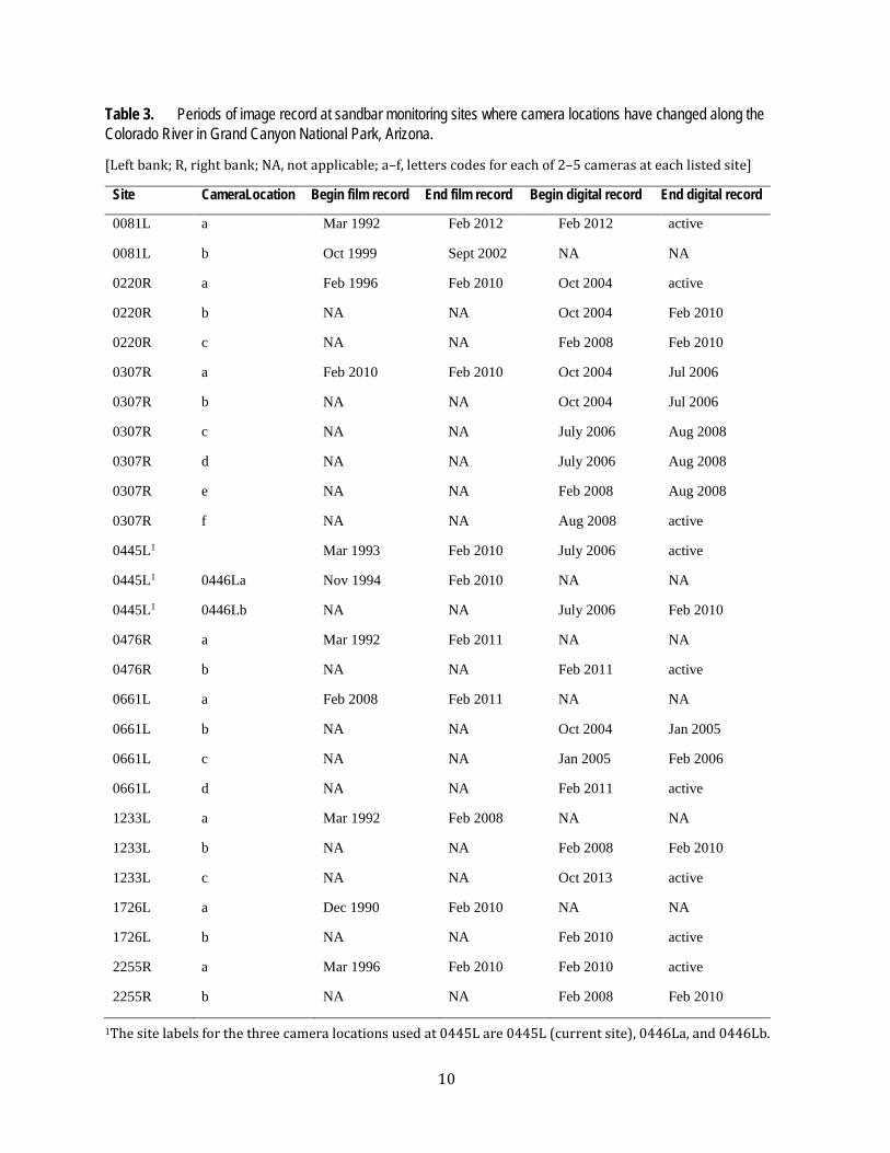
Table 3. Periods of image record at sandbar monitoring sites where camera locations have changed along the Colorado River in Grand Canyon National Park, Arizona.
[Left bank; R, right bank; NA, not applicable; a–f, letters codes for each of 2–5 cameras at each listed site]
Site CameraLocation Begin film record End film record Begin digital record End digital record
0081L a Mar 1992 Feb 2012 Feb 2012 active
0081L b Oct 1999 Sept 2002 NA NA
0220R a Feb 1996 Feb 2010 Oct 2004 active
0220R b NA NA Oct 2004 Feb 2010
0220R c NA NA Feb 2008 Feb 2010
0307R a Feb 2010 Feb 2010 Oct 2004 Jul 2006
0307R b NA NA Oct 2004 Jul 2006
0307R c NA NA July 2006 Aug 2008
0307R d NA NA July 2006 Aug 2008
0307R e NA NA Feb 2008 Aug 2008
0307R f NA NA Aug 2008 active
0445L1 Mar 1993 Feb 2010 July 2006 active
0445L1 0446La Nov 1994 Feb 2010 NA NA
0445L1 0446Lb NA NA July 2006 Feb 2010
0476R a Mar 1992 Feb 2011 NA NA
0476R b NA NA Feb 2011 active
0661L a Feb 2008 Feb 2011 NA NA
0661L b NA NA Oct 2004 Jan 2005
0661L c NA NA Jan 2005 Feb 2006
0661L d NA NA Feb 2011 active
1233L a Mar 1992 Feb 2008 NA NA
1233L b NA NA Feb 2008 Feb 2010
1233L c NA NA Oct 2013 active
1726L a Dec 1990 Feb 2010 NA NA
1726L b NA NA Feb 2010 active
2255R a Mar 1996 Feb 2010 Feb 2010 active
2255R b NA NA Feb 2008 Feb 2010
1The site labels for the three camera locations used at 0445L are 0445L (current site), 0446La, and 0446Lb.

11
All images from the film cameras were professionally scanned and archived on compact disk at the time of film processing. Because these images do not contain Exif information, the digital files (usually high-resolution tiff files) were manually renamed according to the naming convention described above. If the film camera imprinted a timestamp on an image, this time was manually entered into the hhmm part of the filename. If no timestamp was present, 1200 was used. Copies of the original high-resolution tiff files were made at the same web and thumbnail resolutions described above.
A subset of the web-resolution images consisting of one image per day is copied to a web server and these images are made publically available in a map-based viewing application (https://grandcanyon.usgs.gov/gisapps/sandbarphotoviewer/RemoteCameraTimeSeries.html). This application includes images from the film and digital records.
Qualitative Analysis of Sandbar Deposition and Erosion One of the primary uses of the images from the remote cameras is to document the effects of
controlled floods on the sandbar-monitoring sites as soon as possible following each release. As soon as it is possible to retrieve the memory cards from the field, the files are processed and saved online. To provide a summary of sandbar response, the images are viewed by an experienced technician familiar with each site. The technician selects images from before and after the controlled flood that have similar lighting conditions and show the site at approximately the same discharge (fig. 4). The technician then assigns a five-category rating to the sandbar change—large deposition (value of +2), moderate deposition (+1), negligible change (0), moderate erosion (−1), or large erosion (−2).
12
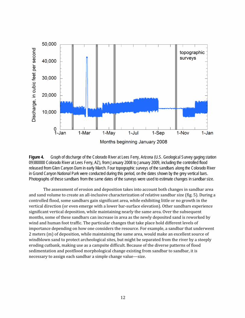
Figure 4. Graph of discharge of the Colorado River at Lees Ferry, Arizona (U.S. Geological Survey gaging station 09380000 Colorado River at Lees Ferry, AZ), from January 2008 to January 2009, including the controlled flood released from Glen Canyon Dam in early March. Four topographic surveys of the sandbars along the Colorado River in Grand Canyon National Park were conducted during this period, on the dates shown by the grey vertical bars. Photographs of these sandbars from the same dates of the surveys were used to estimate changes in sandbar size.
The assessment of erosion and deposition takes into account both changes in sandbar area and sand volume to create an all-inclusive characterization of relative sandbar size (fig. 5). During a controlled flood, some sandbars gain significant area, while exhibiting little or no growth in the vertical direction (or even emerge with a lower bar-surface elevation). Other sandbars experience significant vertical deposition, while maintaining nearly the same area. Over the subsequent months, some of these sandbars can increase in area as the newly deposited sand is reworked by wind and human foot traffic. The particular changes that take place hold different levels of importance depending on how one considers the resource. For example, a sandbar that underwent 2 meters (m) of deposition, while maintaining the same area, would make an excellent source of windblown sand to protect archeological sites, but might be separated from the river by a steeply eroding cutbank, making use as a campsite difficult. Because of the diverse patterns of flood sedimentation and postflood morphological change existing from sandbar to sandbar, it is necessary to assign each sandbar a simple change value—size.
13
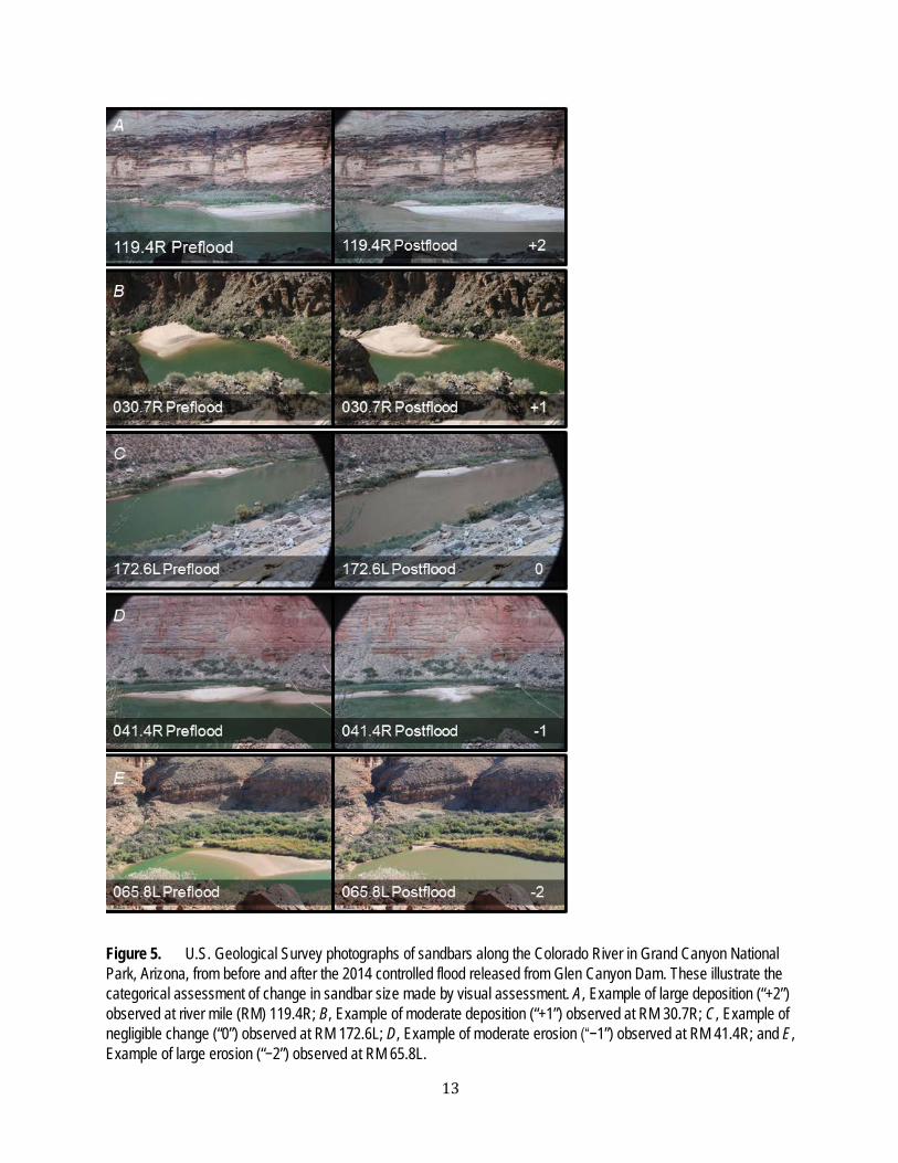
Figure 5. U.S. Geological Survey photographs of sandbars along the Colorado River in Grand Canyon National Park, Arizona, from before and after the 2014 controlled flood released from Glen Canyon Dam. These illustrate the categorical assessment of change in sandbar size made by visual assessment. A, Example of large deposition (“+2”) observed at river mile (RM) 119.4R; B, Example of moderate deposition (“+1”) observed at RM 30.7R; C, Example of negligible change (“0”) observed at RM 172.6L; D, Example of moderate erosion (“−1”) observed at RM 41.4R; and E, Example of large erosion (“−2”) observed at RM 65.8L.

14
Method Validation To validate the qualitative analysis of sandbar change, sandbar photographs were assigned
change values, then compared with topographic-survey data collected over the same period. Four topographic surveys of the sandbar monitoring sites were conducted in 2008. One survey was conducted February 1–18, a month before the controlled flood, and repeat surveys were conducted 1, 2, and 7 months after the controlled flood (April 1–13, May 15–31, and October 15–26). For each of the 22 sites with operational remote cameras in 2008, photographs were extracted for each day a topographic survey was collected (fig. 4). Without knowledge of the changes measured in the surveys, size relative to the condition before the controlled flood was estimated (table 4).
Table 4. Visually estimated changes in sandbar size in remote-camera images taken along the Colorado River in Grand Canyon National Park, Arizona, from March 2008 (before 2008 controlled flood) to April, May, and November 2008.
[Left bank; R, right bank; 2, large deposition; 1, moderate deposition; 0, negligible change; −1, moderate erosion; −2, large erosion; --, no data]
Site ID March to April 2008 March to May 2008 March to November 2008
0081L 1 0 --
0220Ra 2 2 -1
0307Ra 2 2 1
0445L 2 -- 1
0446Lb 2 2 1
0476Ra 2 1 --
0510R 1 1 −1
0559R −1 −1 −2
0688R 2 1 1
0817L 1 1 --
0876L 1 0 −1
0917R 1 1 0
1194R 2 1 0
1227R 2 1 1
1233La −1 -1 −1
1377L 1 1 0
1396R 0 -- 0
1459L 1 0 0
1726La 2 1 --
1946L 1 1 0
15
Site ID March to April 2008 March to May 2008 March to November 2008
2023R 1 0 --
2133L 1 0 0
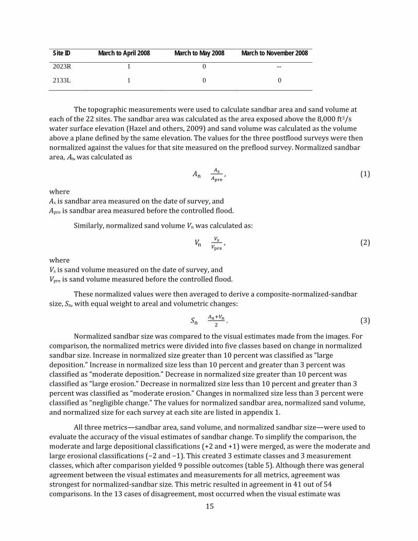
The topographic measurements were used to calculate sandbar area and sand volume at each of the 22 sites. The sandbar area was calculated as the area exposed above the 8,000 ft3/s water surface elevation (Hazel and others, 2009) and sand volume was calculated as the volume above a plane defined by the same elevation. The values for the three postflood surveys were then normalized against the values for that site measured on the preflood survey. Normalized sandbar area, An, was calculated as
𝐴𝐴n = 𝐴𝐴s𝐴𝐴pre
, (1)
where As is sandbar area measured on the date of survey, and Apre is sandbar area measured before the controlled flood.
Similarly, normalized sand volume Vn was calculated as:
𝑉𝑉n = 𝑉𝑉s𝑉𝑉pre
, (2)
where Vs is sand volume measured on the date of survey, and Vpre is sand volume measured before the controlled flood.
These normalized values were then averaged to derive a composite-normalized-sandbar size, Sn, with equal weight to areal and volumetric changes:
𝑆𝑆n = 𝐴𝐴n+𝑉𝑉n2
. (3)
Normalized sandbar size was compared to the visual estimates made from the images. For comparison, the normalized metrics were divided into five classes based on change in normalized sandbar size. Increase in normalized size greater than 10 percent was classified as “large deposition.” Increase in normalized size less than 10 percent and greater than 3 percent was classified as “moderate deposition.” Decrease in normalized size greater than 10 percent was classified as “large erosion.” Decrease in normalized size less than 10 percent and greater than 3 percent was classified as “moderate erosion.” Changes in normalized size less than 3 percent were classified as “negligible change.” The values for normalized sandbar area, normalized sand volume, and normalized size for each survey at each site are listed in appendix 1.
All three metrics—sandbar area, sand volume, and normalized sandbar size—were used to evaluate the accuracy of the visual estimates of sandbar change. To simplify the comparison, the moderate and large depositional classifications (+2 and +1) were merged, as were the moderate and large erosional classifications (−2 and −1). This created 3 estimate classes and 3 measurement classes, which after comparison yielded 9 possible outcomes (table 5). Although there was general agreement between the visual estimates and measurements for all metrics, agreement was strongest for normalized-sandbar size. This metric resulted in agreement in 41 out of 54 comparisons. In the 13 cases of disagreement, most occurred when the visual estimate was
16
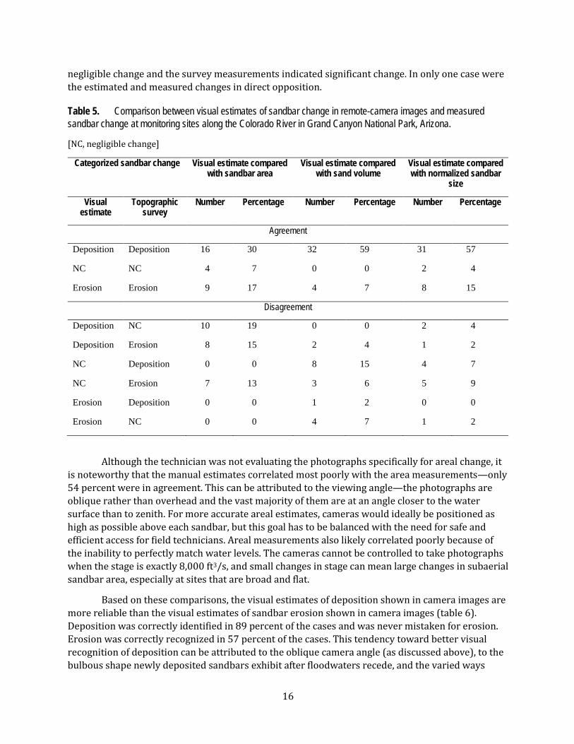
negligible change and the survey measurements indicated significant change. In only one case were the estimated and measured changes in direct opposition.
Table 5. Comparison between visual estimates of sandbar change in remote-camera images and measured sandbar change at monitoring sites along the Colorado River in Grand Canyon National Park, Arizona.
[NC, negligible change]
Categorized sandbar change Visual estimate compared with sandbar area
Visual estimate compared with sand volume
Visual estimate compared with normalized sandbar
size
Visual estimate
Topographic survey
Number Percentage Number Percentage Number Percentage
Agreement
Deposition Deposition 16 30 32 59 31 57
NC NC 4 7 0 0 2 4
Erosion Erosion 9 17 4 7 8 15
Disagreement
Deposition NC 10 19 0 0 2 4
Deposition Erosion 8 15 2 4 1 2
NC Deposition 0 0 8 15 4 7
NC Erosion 7 13 3 6 5 9
Erosion Deposition 0 0 1 2 0 0
Erosion NC 0 0 4 7 1 2
Although the technician was not evaluating the photographs specifically for areal change, it is noteworthy that the manual estimates correlated most poorly with the area measurements—only 54 percent were in agreement. This can be attributed to the viewing angle—the photographs are oblique rather than overhead and the vast majority of them are at an angle closer to the water surface than to zenith. For more accurate areal estimates, cameras would ideally be positioned as high as possible above each sandbar, but this goal has to be balanced with the need for safe and efficient access for field technicians. Areal measurements also likely correlated poorly because of the inability to perfectly match water levels. The cameras cannot be controlled to take photographs when the stage is exactly 8,000 ft3/s, and small changes in stage can mean large changes in subaerial sandbar area, especially at sites that are broad and flat.
Based on these comparisons, the visual estimates of deposition shown in camera images are more reliable than the visual estimates of sandbar erosion shown in camera images (table 6). Deposition was correctly identified in 89 percent of the cases and was never mistaken for erosion. Erosion was correctly recognized in 57 percent of the cases. This tendency toward better visual recognition of deposition can be attributed to the oblique camera angle (as discussed above), to the bulbous shape newly deposited sandbars exhibit after floodwaters recede, and the varied ways

17
sandbars can change as they are subjected to subaerial sediment transport processes and human foot traffic.
Table 6. Matrix of agreement and disagreement between measured change in normalized sandbar size and visually estimated change in sandbar size in remote camera images at monitoring sites along the Colorado River in Grand Canyon National Park, Arizona.
Measured change Percent estimated
Deposition No change Erosion
Deposition 89 11 0
No change 40 40 20
Erosion 7 36 57
This qualitative method of change detection has proven to be a reasonably effective way to assess the effects of controlled-flood events on sandbars along the Colorado River. The manual estimates agreed with survey measurements 76 percent of the time (89 percent for sandbars that aggraded) and wholly disagreed 2 percent of the time (table 5). Compared to traditional ground-survey methods, the low cost, high temporal resolution, and quick data-processing time of visually estimating geomorphic change using remote-camera images make it a useful way to assess such changes.
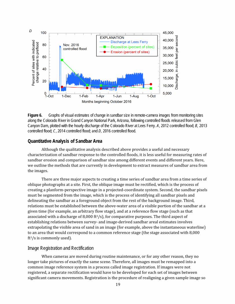
Results of Visual Estimates of Sandbar Change Visual estimates of sandbar change were made for each of the controlled-flood releases from
Glen Canyon Dam in November of 2012, 2013, 2014, and 2016. Although the categories of moderate and large change were used in the assessment (appendix 2), these categories were lumped together for reporting, consistent with the method validation. Immediately following each controlled flood, deposition was observed at 50 percent or more of the monitoring sites (fig. 6), consistent with results from previous controlled floods (Hazel and others, 2010; Schmidt and Grams, 2011). Each controlled flood resulted in erosion at about 10 percent of the monitoring sites. The estimates of sandbar size made from images from February through October indicate that rates of erosion are highest in the first 3 months following each controlled flood. In two of the years (2013 and 2014), 10 to 20 percent of the sites were still larger 11 months after the controlled flood of the previous year. Post-controlled-flood erosion rates were highest in 2015 (following the November 2014 controlled flood), which was also the year of highest annual release volume from Glen Canyon Dam.

18
19
Figure 6. Graphs of visual estimates of change in sandbar size in remote-camera images from monitoring sites along the Colorado River in Grand Canyon National Park, Arizona, following controlled floods released from Glen Canyon Dam, plotted with the hourly discharge of the Colorado River at Lees Ferry. A, 2012 controlled flood; B, 2013 controlled flood; C, 2014 controlled flood; and D, 2016 controlled flood.
Quantitative Analysis of Sandbar Area Although the qualitative analysis described above provides a useful and necessary
characterization of sandbar response to the controlled floods, it is less useful for measuring rates of sandbar erosion and comparison of sandbar size among different events and different years. Here, we outline the methods that are currently in development to extract measures of sandbar area from the images.
There are three major aspects to creating a time series of sandbar area from a time series of oblique photographs at a site. First, the oblique image must be rectified, which is the process of creating a planform-perspective image in a projected-coordinate system. Second, the sandbar pixels must be segmented from the image, which is the process of identifying all sandbar pixels and delineating the sandbar as a foreground object from the rest of the background image. Third, relations must be established between the above-water area of a visible portion of the sandbar at a given time (for example, an arbitrary flow stage), and at a reference flow stage (such as that associated with a discharge of 8,000 ft3/s), for comparative purposes. The third aspect of establishing relations between survey- and image-derived sandbar areal estimates involves extrapolating the visible area of sand in an image (for example, above the instantaneous waterline) to an area that would correspond to a common reference stage (the stage associated with 8,000 ft3/s is commonly used).
Image Registration and Rectification When cameras are moved during routine maintenance, or for any other reason, they no
longer take pictures of exactly the same scene. Therefore, all images must be remapped into a common image reference system in a process called image registration. If images were not registered, a separate rectification would have to be developed for each set of images between significant camera movements. Registration is the procedure of realigning a given sample image so

20
that it has the same image-coordinate-reference frame as a single reference image. The purpose is to place all images for a given site in a common image-reference frame. Our approach is to find the translation of the sample image in two dimensions (x and y) relative to a reference image, using frequency domain methods. First, we calculate the cross-correlation function between the master and given sample image, by means of the two-dimensional fast Fourier transform (2D-FFT) and locating its peak (fig. 7). An example Python program for this computation is given in appendix 3. The peak in two dimensions represents the shift in x and y locations, which are accordingly applied to the sample image to register it (fig. 7). It is therefore a “translation only,” frequency-domain image transformation. It is reasonably fast (an image takes only as long as a few seconds to process, on a single >2 gigahertz computer processor) and responds well to lighting variations. We tested another approach in the spatial domain, which involved finding translations based on the pixel locations of common-scale invariant features seen in both master and sample images, implementing the scale invariant feature transform (SIFT; Lowe, 2004) algorithm for detecting identical features in pairs of images, using random sample consensus (RANSAC; Fischler and Bowles, 1981) to filter spurious features, according to the algorithm detailed in Solem (2012). However, the 2D-FFT approach was deemed superior, both in accuracy and speed.
Figure 7. Example of the image-registration workflow used for sandbar monitoring along the Colorado River in Grand Canyon National Park, Arizona. A, a reference photograph against which all other images from remote cameras at a site are compared; B, a given sample (unregistered) image; C, the two-dimensional cross-correlation between reference and sample image, identifying the peak, the location of which represents the shift in two horizontal directions; D, the registered sample image; and E, three images showing a small subsection of the image from, top, the reference; middle, the unregistered sample; and bottom, the registered sample images.

21
When a set of images from a particular camera system have been registered, these images are then rectified. This step involves computation of a transformation matrix from the pixel coordinates in the oblique image to real-world coordinates to create a planform image in a projected-coordinate system (fig. 8). The resulting transformed image is referred to as the rectified image. The approach we have adopted is to find the homography between two sets of points—(1) ground-control points (GCPs) in an image reference system (their pixel coordinates) and (2) their corresponding real world coordinates. Note that only two-dimensional points [x,y] are considered. The same transformation matrix will apply to all images from a camera deployment observing a particular site.
Figure 8. Example of the image rectification workflow used for sandbar monitoring along the Colorado River in Grand Canyon National Park, Arizona. A, a registered oblique photograph from a remote camera; B, the rectified image; C, the rectified georeferenced image overlaying a 2013 aerial image; and D, the surveyed extent of the sandbar at that location and time (shown in red), overlaying the rectified georeferenced image.
First, we find the perspective transformation matrix, which is a 3×3 matrix, h, which describes the mapping or image coordinates [x',y'] to real world coordinates [x,y] in a projected coordinate system using the following equation, where w is a scalar:
�𝒘𝒘𝒘𝒘𝒘𝒘𝒘𝒘𝒘𝒘� = �
𝒉𝒉𝟏𝟏𝟏𝟏 𝒉𝒉𝟏𝟏𝟏𝟏 𝒉𝒉𝟏𝟏𝟏𝟏𝒉𝒉𝟏𝟏𝟏𝟏 𝒉𝒉𝟏𝟏𝟏𝟏 𝒉𝒉𝟏𝟏𝟏𝟏𝒉𝒉𝟏𝟏𝟏𝟏 𝒉𝒉𝟏𝟏𝟏𝟏 𝒉𝒉𝟏𝟏𝟏𝟏
� �𝒘𝒘′𝒘𝒘′𝟏𝟏� . (4)
Matrix h is found by establishing the correspondences between at least n=4 real-world coordinate pairs [x,y] and their equivalent image coordinates [x',y']. From equation (4) we can write the following homogenous linear system, Ah=0 such that:
22
⎣⎢⎢⎢⎡𝒘𝒘𝟏𝟏 𝒘𝒘𝟏𝟏 𝟏𝟏 𝟎𝟎 𝟎𝟎 𝟎𝟎 −𝒘𝒘𝟏𝟏′ 𝒘𝒘𝟏𝟏 −𝒘𝒘𝟏𝟏′ 𝒘𝒘𝟏𝟏 −𝒘𝒘𝟏𝟏′
𝟎𝟎 𝟎𝟎 𝟎𝟎 𝒘𝒘𝟏𝟏 𝒘𝒘𝟏𝟏 𝟏𝟏 −𝒘𝒘𝟏𝟏′ 𝒘𝒘𝟏𝟏 −𝒘𝒘𝟏𝟏′ 𝒘𝒘𝟏𝟏 −𝒘𝒘𝟏𝟏′⋮ ⋮ ⋮ ⋮ ⋮ ⋮ ⋮ ⋮ ⋮𝒘𝒘𝒏𝒏 𝒘𝒘𝒏𝒏 𝟏𝟏 𝟎𝟎 𝟎𝟎 𝟎𝟎 −𝒘𝒘𝒏𝒏′ 𝒘𝒘𝒏𝒏 −𝒘𝒘𝒏𝒏′ 𝒘𝒘𝒏𝒏 −𝒘𝒘𝒏𝒏′𝟎𝟎 𝟎𝟎 𝟎𝟎 𝒘𝒘𝒏𝒏 𝒘𝒘𝒏𝒏 𝟏𝟏 −𝒘𝒘𝒏𝒏′ 𝒘𝒘𝒏𝒏 −𝒘𝒘𝒏𝒏′ 𝒘𝒘𝒏𝒏 −𝒘𝒘𝒏𝒏′ ⎦
⎥⎥⎥⎤
⎣⎢⎢⎢⎢⎢⎢⎢⎢⎡𝒉𝒉𝟏𝟏𝟏𝟏𝒉𝒉𝟏𝟏𝟏𝟏𝒉𝒉𝟏𝟏𝟏𝟏𝒉𝒉𝟏𝟏𝟏𝟏𝒉𝒉𝟏𝟏𝟏𝟏𝒉𝒉𝟏𝟏𝟏𝟏𝒉𝒉𝟏𝟏𝟏𝟏𝒉𝒉𝟏𝟏𝟏𝟏𝒉𝒉𝟏𝟏𝟏𝟏⎦
⎥⎥⎥⎥⎥⎥⎥⎥⎤
=
⎣⎢⎢⎢⎡𝟎𝟎𝟎𝟎⋮𝟎𝟎𝟎𝟎⎦⎥⎥⎥⎤ . (5)
This is an optimization problem with a least-squares solution given by:
𝐦𝐦𝐦𝐦𝐦𝐦‖𝑨𝑨𝒉𝒉− 𝟎𝟎‖𝟏𝟏 , (6)
which is solved as the eigenvector of ATA with the smallest eigenvalue, where T denotes matrix transpose. The problem may be formally stated, where
𝑒𝑒→𝜆𝜆
and 𝜆𝜆 are eigenvectors and eigenvalues,
respectively, of matrix ATA
min𝜆𝜆𝐴𝐴𝑇𝑇𝐴𝐴 𝑒𝑒
→𝜆𝜆 = 𝜆𝜆 𝑒𝑒
→𝜆𝜆
which, using the identity I we may rewrite as a null-space problem:
𝐴𝐴𝑇𝑇𝐴𝐴 𝑒𝑒→𝜆𝜆 = 𝐼𝐼𝜆𝜆 𝑒𝑒
→𝜆𝜆 ⇒ (𝐴𝐴𝑇𝑇𝐴𝐴 − 𝜆𝜆𝐼𝐼) 𝑒𝑒
→𝜆𝜆 = 0
→
This has a solution if |𝐴𝐴𝑇𝑇𝐴𝐴 − 𝜆𝜆𝐼𝐼| = 0. The eigenvalues are found as the roots of the characteristic polynomial 𝑝𝑝(𝜆𝜆) = |𝐴𝐴𝑇𝑇𝐴𝐴 − 𝜆𝜆𝐼𝐼| and the eigenvectors associated with each eigenvalue 𝜆𝜆𝑖𝑖 are the vectors in the null space of the matrix (𝐴𝐴𝑇𝑇𝐴𝐴 − 𝜆𝜆𝑖𝑖𝐼𝐼).
Once the transformation matrix has been obtained, an oblique image is rectified using the OpenCV library (http://opencv.org/) function warpPerspective (OpenCV, 2014).
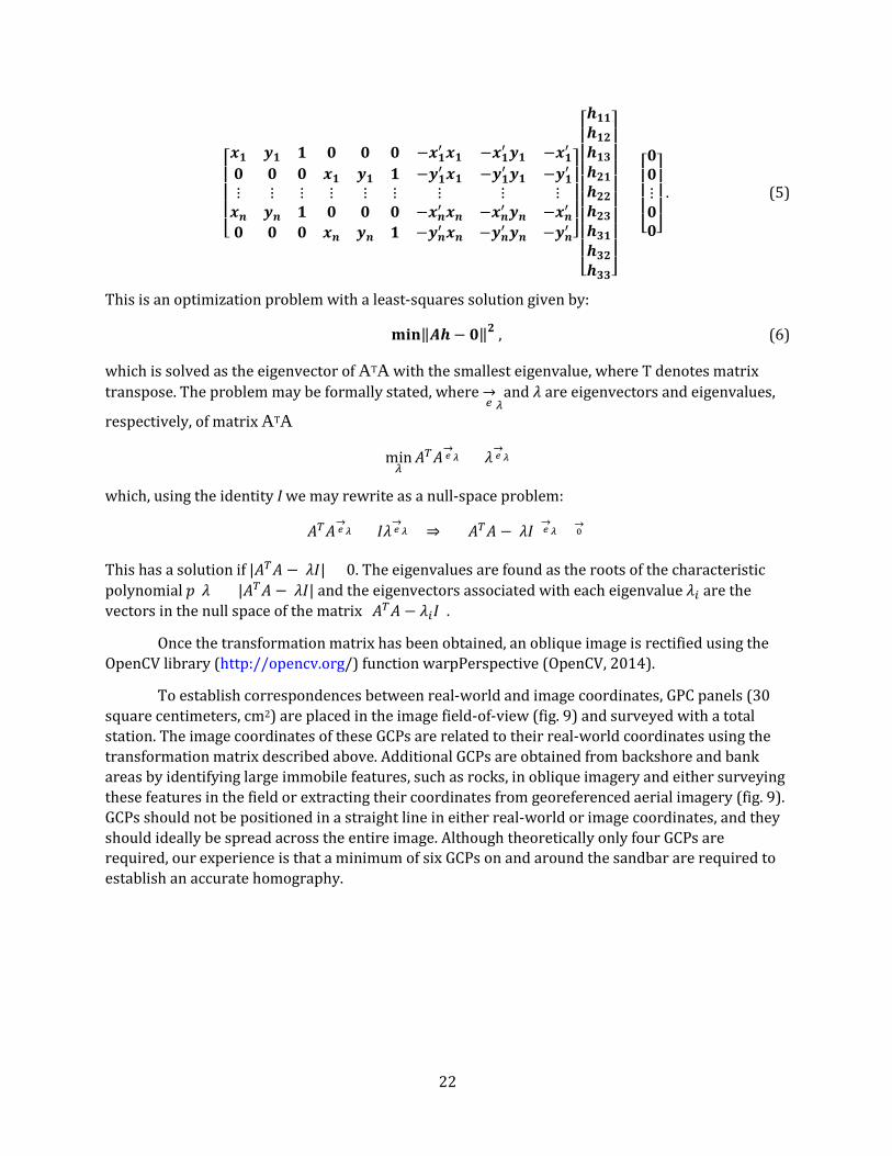
To establish correspondences between real-world and image coordinates, GPC panels (30 square centimeters, cm2) are placed in the image field-of-view (fig. 9) and surveyed with a total station. The image coordinates of these GCPs are related to their real-world coordinates using the transformation matrix described above. Additional GCPs are obtained from backshore and bank areas by identifying large immobile features, such as rocks, in oblique imagery and either surveying these features in the field or extracting their coordinates from georeferenced aerial imagery (fig. 9). GCPs should not be positioned in a straight line in either real-world or image coordinates, and they should ideally be spread across the entire image. Although theoretically only four GCPs are required, our experience is that a minimum of six GCPs on and around the sandbar are required to establish an accurate homography.
23
Figure 9. Example oblique photograph taken by a remote camera used for sandbar monitoring along the Colorado River in Grand Canyon National Park, Arizona. Locations of checkerboard panels (within black circles and inset) used to build a homography between real-world and image coordinates are shown. Survey tripods and other objects with a known horizontal (easting, northing) location, such as the tripod on the far left of the scene (red circle), may also be used to constrain or check a solution.
Delineation of Sandbar Area Below we describe the process of segmenting the sandbar from the background in an
oblique (unrectified) image. When the coordinates associated with the boundary of the sandbar have been extracted, these coordinates are transformed into a projected coordinate system using the same transformation matrix that is used to rectify the image. Delineating the sandbar from the rectified image would also be possible, but because the oblique image contains more sand pixels than the rectified version, the sandbar outline is better resolved using the oblique image. In addition, keeping sandbar boundary coordinates in an image reference frame means that the segmentation need only be carried out once, even if the transformation matrix is changed (for example, if new GCPs become available and the homography is recomputed).
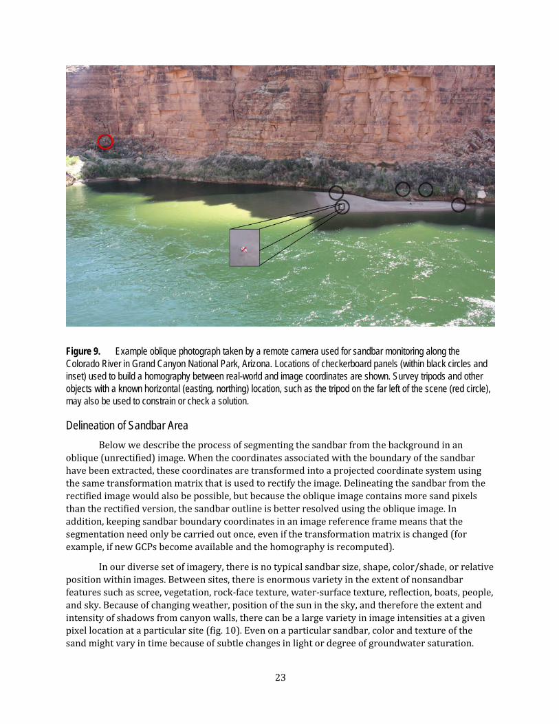
In our diverse set of imagery, there is no typical sandbar size, shape, color/shade, or relative position within images. Between sites, there is enormous variety in the extent of nonsandbar features such as scree, vegetation, rock-face texture, water-surface texture, reflection, boats, people, and sky. Because of changing weather, position of the sun in the sky, and therefore the extent and intensity of shadows from canyon walls, there can be a large variety in image intensities at a given pixel location at a particular site (fig. 10). Even on a particular sandbar, color and texture of the sand might vary in time because of subtle changes in light or degree of groundwater saturation.
24
These factors make a single approach to automatically detecting and segmenting sandbars, with sufficient accuracy, an extremely challenging computer vision task.
Figure 10. Time series of oblique imagery from a sandbar monitoring site (RC0307R) along the Colorado River in Grand Canyon National Park, Arizona, taken during the November 2012 controlled flood release from Glen Canyon Dam. Time increases from left to right and from top to bottom.
Any algorithm used to identify sand pixels might be (in order of preference) fully automated (unsupervised), semiautomated (supervised), or manual. We have developed a supervised approach, based on considering the trade-off between accuracy and speed (a fully manual approach is highly accurate but too slow and an unsupervised approach is fast but not sufficiently consistent in its accuracy). An interactive graphical program, Remote Camera Sandbar Segmentation (RCSandSeg), has been developed in the Python programming language that allows the user to select a set of images, filter them by date/time and stage, interactively segment the sandbar from the image, and store the coordinates of the bar outline. This program is available as a GitHub repository at https://github.com/dbuscombe-usgs/RCSandSeg (Buscombe, 2017). The sandbar
25
outline is extracted using image processing techniques that are relatively invariant to large changes in light and shadow, water, color, and the spectrum of image textures associated with different surface types. These image-processing procedures are detailed below. An operator supervises the process and carries out on-the-fly quality control. Each image takes 10–60 seconds to process by an experienced operator.
This partially automated workflow results in accurate sandbar outlines and areas. However, given the large and ever-growing database of images (at present consisting of >488,000 images), a fully automated workflow will eventually be necessary. Because of the extreme difficulties associated with identifying sand pixels based on color and texture metrics alone, further work is required to develop a completely automated (unsupervised) sandbar segmentation that is as reliable as the partially supervised method detailed above. Several approaches are currently being investigated.
The RCSandSeg Program RCSandSeg (Buscombe, 2017) is a Python program with a graphical user interface (GUI) that
enables a user to interactively segment a sandbar from an image (a registered image still in an image reference frame, unrectified) or series of images. The user selects a set of images, and interactively segments them, one by one. The results from each image are saved in a binary Python format (a so-called pickled object), one file per image. There are three tabs in the program, each with slightly different functionality (fig. 11). The first (gold) tab allows the user to select multiple arbitrary files, make a movie of them (which greatly facilitates the visual detection of sandbar changes over time), and (or) process them. The act of processing in this case refers to the interactive segmentation that is explained below. The second (green) tab allows the user to find images from the database, based on site or camera deployment, date range, time of day (including the ideal time for a given site, predetermined based on average lighting conditions at a particular site), and discharge level (fig. 12). The discharge at a particular site is then estimated using empirical relations developed for each site based on the average lag time between the discharge at the nearest upstream gage. These relations were constructed by running the Wiele and Griffin (1998) unsteady flow model over the full range of flows for each of the five Colorado River gages upstream from the study sites. The predicted hydrograph at the cross section closest to each site was then cross correlated with the hydrograph of the nearest upstream gage (fig. 13). The program will find images within a user-specified tolerance of the desired discharge level at the nearest gage (the default is ±100 ft3/s). Again, once the images are found based on the user’s criteria, the user can process and make a movie of these images (the movie this time will include a plot of the discharge curve for the selected date range). The third (purple) tab allows the user to find images from the database, based on site/deployment, date range, and time of day (including the ideal time for a given site). In other words, it does the same as the green tab, except the specification of discharge.

26
Figure 11. Screenshots from the RCSandSeg program (Buscombe, 2017) used to process remote-camera images for sandbar monitoring along the Colorado River in Grand Canyon National Park, Arizona. A, The user launches the program and selects a working directory, subdirectories contain images per camera site; B, the gold tab of the program allows the user to select and process arbitrary collections of images; C, the green tab of the program allows the user to select and process imagery based on site, date range, discharge level, and time of day; and D, the purple tab of the program allows the user to select and process imagery based on site, date range, and time of day.
27
Figure 12. Screenshots from the green tab of the RCSandSeg program (Buscombe, 2017) used to process remote-camera images for sandbar monitoring along the Colorado River in Grand Canyon National Park, Arizona. A, View of the terminal window that prints activity to screen; B, the graphical user interface (GUI) window; C, the instructions window; and D, a window showing a list of files that correspond with the filtering criteria set in the GUI window.
Figure 13. Graph of time lag, in hours, between discharge at each remote-camera site (marker) and the nearest upstream gaging station (dashed lines, U.S. Geological Survey gaging stations identifiers shown at top) along the Colorado River in Grand Canyon National Park, Arizona. The lines and equations are least-squares linear models. River miles are distance in miles along the channel centerline downstream from Lees Ferry.

28
The program is used in the following way. A window appears containing the image. The user draws a box around the sandbar by dragging the mouse over the image, then presses the “n” key on the keyboard. The program makes an initial estimate of the sandbar location within the box and displays this within a second window (fig. 14). When the user presses “n” again, the program updates its estimate. After a few presses of the “n” key, the estimate of the sandbar location no longer changes. At that point, the user can accept the sandbar segmentation by visually comparing the segmentation with the input image and making a subjective decision about whether or not it is of acceptable accuracy. Sometimes, no additional input is necessary (fig. 14A). Then, the program saves the result (the coordinates, in the image reference frame, of the sandbar boundary) and moves on to the next image. If the segmentation is unsatisfactory, the user gives the program new information that allows it to improve its estimate. This is done by specifying what is foreground (sandbar) or background in the image, by drawing on the image with the mouse. Foreground marking is carried out by pressing the “1” key and then drawing on the image where there is sandbar the program has missed. Background marking is carried out by pressing the “0” key, then drawing on the image where there is no sandbar. The program refines its estimate of the sandbar location based on this new information (fig. 14B).

29
Figure 14. Example interactive segmentation in the RCSandSeg program (Buscombe, 2017) used to process remote-camera images for sandbar monitoring along the Colorado River in Grand Canyon National Park, Arizona. A, The user draws a blue bounding box around an image (left), and the resulting segmentation (right) is perfect; B, the user draws a bounding box around the bar in this image with strong shadows, and annotates foreground (white) and background (black) with the mouse (left). The resulting segmentation is on the right.
The program is built on the GrabCut algorithm (Rother and others, 2004) which is a powerful and widely used interactive image segmentation approach (Szeliski, 2010). Starting with a user-specified bounding box around the sandbar to be segmented, the algorithm estimates the color distribution of the pixels within the bounding box, and also that of the background (outside the bounding box), using a Gaussian mixture model (Bishop, 2006). A graph is built, in which each node represents a unique pixel in the image. Two additional nodes are created, the “source” and “sink” nodes, representing the foreground and background, respectively, and which are initially connected to every other node. The image is segmented by connecting each node to either the source or sink node. Any information provided by the user (the foreground/background annotations) are set as hard constraints (individual nodes are assigned a label which cannot change). All other nodes are assigned a probability of being in the foreground or background. An energy cost function is incorporated into the graph as weights between pairs of pixel nodes and between pixel nodes and
30
source or sink nodes. Similarly colored neighboring pixels are encouraged to have the same label by assigning relatively large weights between their nodes. Strong gradients in color between pairs of pixels are given relatively small weights. A min-cut/max-flow algorithm (Boykov and others, 2001) is used to cut the graph. The algorithm determines the minimum cost cut that will separate the source and sink nodes. The cost of a cut is the sum of the weights of the links between nodes that are cut. To segment the image, all nodes connected to the source become foreground and all nodes connected to the sink become background. Segmentations are further refined by the user by pointing out misclassified regions and rerunning the energy function (assigning values to weights) and recutting the graph.
Sandbar Area at RC0307 Between October 2009 and October 2015 Site RC0307 (camera location f), which is located 30.7 miles downstream of Lees Ferry, AZ,
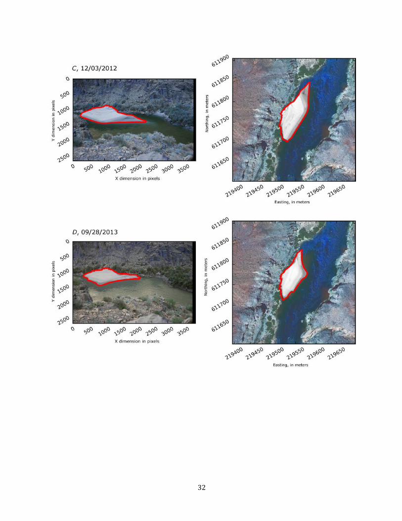
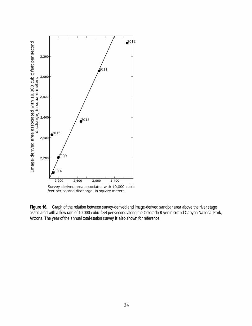
in Lower Marble Canyon, was chosen to demonstrate the process of estimating time series of sandbar area from a sequence of oblique photographs. Registered images taken between October 2009 and October 2015 when the river discharge was 10,000±50 ft3/s were selected. Out of this subsample of registered imagery, those images taken closest in time to a total station survey were processed using RCSandSeg to extract sandbar outline. The images and sandbar outline were subsequently rectified (fig. 15) and sandbar areas estimated using the Shoelace formula (Braden, 1986), the implementation of which is shown in appendix 4. The comparison between estimated sandbar areas and equivalent survey areas (above the stage associated with 10,000 ft3/s) was satisfactory (fig. 16), with a coefficient of determination, R2, of 0.907, and a root-mean-square error (RMSE) of 212.83 square meters (m2), which is equivalent to an average error of 8 percent. The main sources of error are (1) actual differences in sandbar area due to physical processes occurring between image time and survey time (2009: 19 days; 2011: 67 days; 2012: 59 days; 2013:5 days; 2014: 1 day; and 2015: 4 days); (2) error in the digitized outline of the sandbar output from the RCSandSeg program; (3) discrepancy in sandbar area associated with imprecision in flow stage; (4) error in the registration process; (5) error in the rectification process; and (6) error in the total-station survey-derived sandbar area. All of these sources of error are planned to be investigated, quantified and, where possible, minimized, in subsequent studies. Having established a reasonable relation between observed and image-derived sandbar area above the 10,000 ft3/s stage, the remaining images were processed using RCSandSeg and sandbar areas estimated. Figure 17 shows the results from that analysis, within the context of the survey-derived sandbar area time series that extends back to 1990 (Hazel and others, 2010). It is apparent that very significant changes to sandbar area occur on a subannual timescale, as previously reported by Cluer (1995). Indeed, close inspection of the time series reveals times where highly episodic large-magnitude erosion of sandbars occurs over just a few days or weeks. Some of these events are shown graphically in figure 18.
31
32

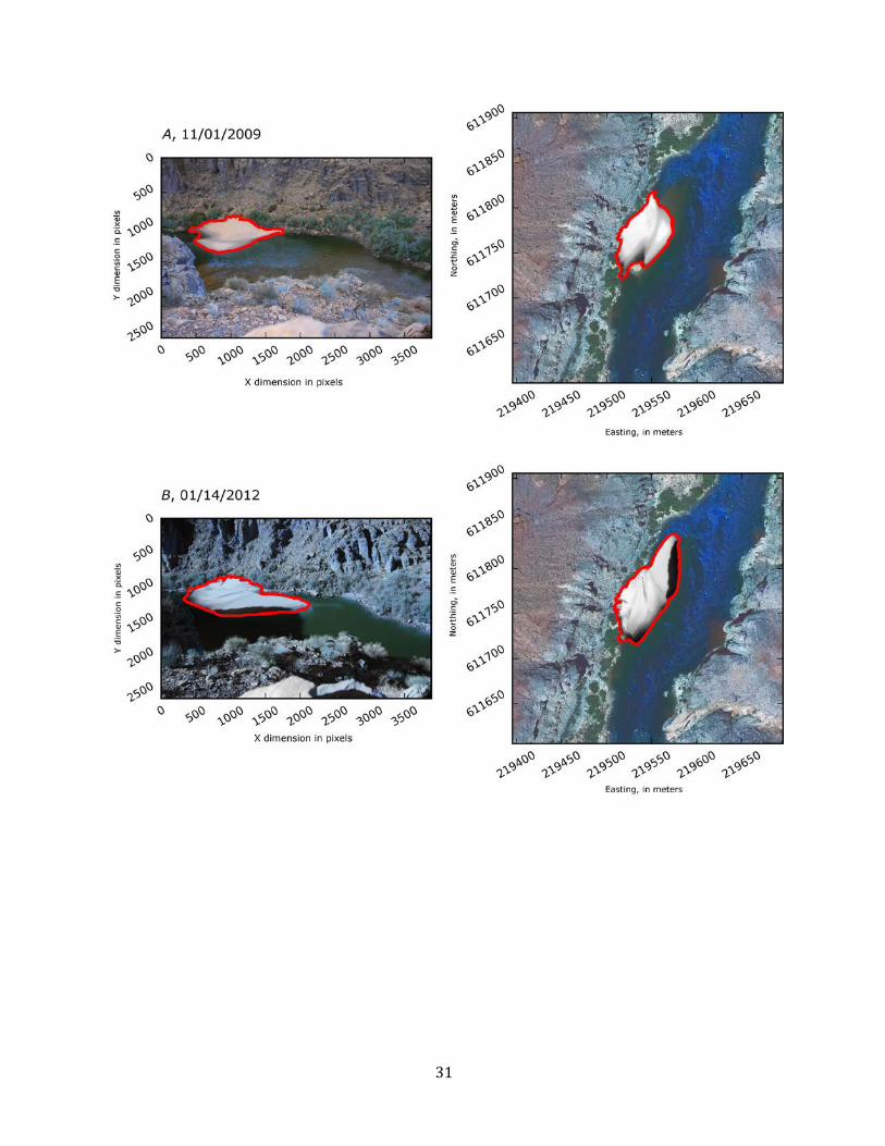
33
Figure 15. Time series of oblique remote-camera imagery (A–F, left), with identified sandbar outlines (red lines), used for sandbar monitoring along the Colorado River in Grand Canyon National Park, Arizona, and their corresponding rectified image overlaying aerial imagery from May 2013 (right). This time series is associated closest in time to total-station surveys, is near the river stage associated with a flow rate of 10,000 cubic feet per second, and the derived sandbar areas are used to construct figure 16. Date format is two-digit month and day followed by year (MM/DD/YEAR).
34
Figure 16. Graph of the relation between survey-derived and image-derived sandbar area above the river stage associated with a flow rate of 10,000 cubic feet per second along the Colorado River in Grand Canyon National Park, Arizona. The year of the annual total-station survey is also shown for reference.

35
Figure 17. Graphs showing (A) time series since 1990 of total-station survey-derived (black circles) and image-derived (red dots) sandbar areas above the river stage associated with a flow rate of 10,000 cubic feet per second along the Colorado River in Grand Canyon National Park, Arizona, and (B) a close-up of the period 2009–2015 (inclusive).

36
Figure 18. Images showing comparisons between rectified sandbars (overlaying 2013 aerial imagery) used for sandbar monitoring along the Colorado River in Grand Canyon National Park, before and after an erosional event or period, showing the magnitudes and time-scales of episodic high-magnitude sandbar erosion. Date format is two-digit month and day followed by year (MM/DD/YEAR).

37
References Cited Alvarez, L.V., and Schmeeckle, M.W., 2013, Erosion of river sandbars by diurnal stage fluctuations in
the Colorado River in the Marble and Grand Canyons—Full-scale laboratory experiments: River Research and Applications, v. 29, no. 7, p. 839–854, https://doi.org/10.1002/rra.2576.
Beus, S.S., and Avery, C.C., 1993, The influence of variable discharge regimes on Colorado River sand bars below Glen Canyon Dam: Flagstaff, Ariz., Northern Arizona University, 554 p, accessed January 25, 2018, at https://www.gcmrc.gov/library/reports/physical/Fine_Sed/beus1993.pdf.
Bishop, C.M., 2006, Pattern recognition and machine learning: New York, Springer Science and Business Media, 738 p.
Bogle, R., Velasco, M., and Vogel, J., 2013, An automated digital imaging system for environmental monitoring applications: U.S. Geological Survey Open-File Report 2012–1271, 18 p., https://pubs.er.usgs.gov/publication/ofr20121271.
Boykov, Y., Veksler, O., and Zabih, R., 2001, Fast approximate energy minimization via graph cuts: IEEE Transactions on Pattern Analysis and Machine Intelligence, v. 23, no. 11, p. 1222–1239.
Braden, B., 1986, The surveyor’s area formula: The College Mathematics Journal, v. 17, no. 4, p. 326–337.
Budhu, M., and Gobin, R., 1995, Seepage-induced slope failures on sandbars in Grand Canyon: Journal of Geotechnical Engineering, v. 121, no. 8, p. 601–609.
Buscombe, D., 2017, dbuscombe-usgs/RCSandSeg—First Release of RCSandSeg (version 0.0.2): Zenodo web page, accessed June 15, 2016, at http://doi.org/10.5281/zenodo.1043595.
Cluer, B.L., 1995, Cyclic fluvial processes and bias in environmental monitoring, Colorado River in Grand Canyon: The Journal of Geology, v. 103, no. 4, p. 411–421.
Converse, Y.K., Hawkins, C.P., and Valdez, R.A., 1998, Habitat relationships of subadult humpback chub in the Colorado River through Grand Canyon—Spatial variability and implications of flow regulation: Regulated Rivers—Research & Management, v. 14, no. 3, p. 267–284.
Dolan, R., Howard, A., and Gallenson, A., 1974, Man’s impact on the Colorado River in the Grand Canyon—The Grand Canyon is being affected both by the vastly changed Colorado River and by the increased presence of man: American Scientist, v. 62, no. 4, p. 393–401.
East, A.E., Collins, B.D., Sankey, J.B., Corbett, S.C., Fairley, H.C., and Caster, J., 2016, Conditions and processes affecting sand resources at archeological sites in the Colorado River corridor below Glen Canyon Dam, Arizona: U.S. Geological Survey Professional Paper 1825, 104 p., https://doi.org/10.3133/pp1825.
Fischler, M.A., and Bolles, R.C., 1981, Random sample consensus—A paradigm for model fitting with applications to image analysis and automated cartography: Communications of the ACM [Association for Computing Machinery], v. 24, no. 6, p. 381–395, https://doi.org/10.1145/358669.358692.
Grams, P.E., Schmidt, J.C., Wright, S.A., Topping, D.J., Melis, T.S., and Rubin, D.M., 2015, Building sandbars in the Grand Canyon: EOS, Transactions of the American Geophysical Union, v. 96, p. 1–11, https://doi.org/10.1029/2015EO030349.
38
Hazel, J.E., Jr., Grams, P.E., Schmidt, J.C., and Kaplinski, M., 2010, Sandbar response in Marble and Grand Canyons, Arizona, following the 2008 high-flow experiment on the Colorado River: U.S. Geological Survey Scientific Investigations Report 2010–5015, 52 p., https://pubs.er.usgs.gov/publication/sir20105015.
Hazel, J.E., Kaplinski, M., Parnell, R., Manone, M., and Dale, A., 1999, Topographic and bathymetric changes at thirty-three long-term study sites, in Webb, R.H., Schmidt, J.C., Valdez, R.A., and Marzolf, G.R., eds., The controlled flood in Grand Canyon: Washington D.C., American Geophysical Union, p. 161–183.
Howard, A., and Dolan, R., 1981, Geomorphology of the Colorado River in the Grand Canyon: The Journal of Geology, v. 89, no. 3, p. 269–298.
Kearsley, L.H., Schmidt, J.C., and Warren, K.D., 1994, Effects of Glen Canyon Dam on Colorado River sand deposits used as campsites in Grand Canyon National Park, USA: River Research and Applications, v. 9, no. 3, p. 137–149.
Lowe, D.G., 2004, Distinctive image features from scale-invariant keypoints: International Journal of Computer Vision, v. 60, no. 2, p. 91–110, https:/doi.org/10.1023/B:VISI.0000029664.99615.94.
OpenCV, 2014, Geometric image transformations—warpPerspective: OpenCV web page, accessed January 10, 2018, at http://docs.opencv.org/2.4/modules/imgproc/doc/geometric_transformations.html.
Ralston, B.E., 2005, Riparian vegetation and associated wildlife, in Gloss, S.P., Lovich, J.E., and Melis, T.S., eds., The state of the Colorado River ecosystem in Grand Canyon: U.S. Geological Survey Circular 1282, p. 103–121.
Ross, R.P., and Grams, P.E., 2015, Long-term monitoring of sandbars on the Colorado River in Grand Canyon using remote sensing: Proceedings of the 3rd Joint Federal Interagency Conference, p. 86–96.
Rother, C., Kolmogorov, V., and Blake, A., 2004, GrabCut—Interactive foreground extraction using iterated graph cuts: ACM [Association for Computing Machinery] Transactions on Graphics, v. 23, no. 3, p. 309–314.
Schmidt, J.C., 1990, Recirculating flow and sedimentation in the Colorado River in Grand Canyon, Arizona: The Journal of Geology, v. 98, no. 5, p. 709–724.
Schmidt, J.C., and Graf, J.B., 1990, Aggradation and degradation of alluvial sand deposits, 1965 to 1986, Colorado River, Grand Canyon National Park, Arizona: U.S. Geological Survey Professional Paper 1493, 74 p., https://pubs.er.usgs.gov/publication/pp1493.
Schmidt, J.C., and Grams, P.E., 2011, The high flows—physical science results, in Melis, T.S., ed., Effects of three high-flow experiments on the Colorado River ecosystem downstream from Glen Canyon Dam, Arizona: U.S. Geological Survey Circular 1366, p. 53–91, https://pubs.er.usgs.gov/publication/cir1366.
Schmidt, J.C., Grams, P.E., and Leschin, M.F., 1999, Variation in the magnitude and style of deposition and erosion in three long (8–12 km) reaches as determined by photographic analysis, in Webb, R.H., Schmidt, J.C., Valdez, R.A., and Marzolf, G.R., eds., The controlled flood in Grand Canyon: Washington D.C., American Geophysical Union, p. 185–203.

39
Schmidt, J.C., Topping, D.J., Grams, P.E., and Hazel Jr., J.E., 2004, System-wide changes in the distribution of fine sediment in the Colorado River corridor between Glen Canyon Dam and Bright Angel Creek, Arizona: Final report from Utah State University to Grand Canyon Monitoring and Research Center, 107p., accessed January 25, 2018, at https://www.gcmrc.gov/library/reports/Physical/Fine_Sed/Schmidt2004.pdf.
Solem, J.E., 2012, Programming computer vision with Python—Tools and algorithms for analyzing images: O’Reilly Media, Inc., 264 p.
Stewart, W., Larkin, K., Orland, B., and Anderson, D., 2003, Boater preferences for beach characteristics downstream from Glen Canyon Dam, Arizona: Journal of Environmental Management, v. 69, no. 2, p. 201–211.
Szeliski, R., 2010, Computer vision—algorithms and applications: New York, Springer Science and Business Media, 957 p.
U.S. Department of the Interior, 2012, Environmental assessment—Development and implementation of a protocol for high-flow experimental releases from Glen Canyon Dam, Arizona, 2011 through 2020: Salt Lake City, Utah, U.S. Department of the Interior Bureau of Reclamation, 546 p.
Valdez, R.A., and Ryel, R.J., 1995, Life history and ecology of the Humpback Chub (Gila cypha) in the Colorado River, Grand Canyon, Arizona: U.S. Bureau of Reclamation, Glen Canyon Environmental Studies, 328 p., accessed January 25, 2018, at https://www.gcmrc.gov/library/reports/biological/Fish_studies/Biowest/Valdez1995f.pdf.
Webb, R.H., Schmidt, J.C., Valdez, R.A., and Marzolf, G.R. eds., The controlled flood in Grand Canyon: Washington D.C., American Geophysical Union, 367 p.
Wiele, S.M., and Griffin, E.R., 1998, Modifications to a one-dimensional model of unsteady flow in the Colorado River through the Grand Canyon: U.S. Geological Survey Water-Resources Investigations Report 97–4046, 17 p., https://pubs.er.usgs.gov/publication/wri974046.
Wright, S.A., and Kennedy, T.A., 2011, Science-based strategies for future high-flow experiments at Glen Canyon Dam, in Melis, T.S., ed., Effects of three high-flow experiments on the Colorado River ecosystem downstream from Glen Canyon Dam, Arizona: U.S. Geological Survey Circular 1366, p. 127–147, https://pubs.er.usgs.gov/publication/cir1366.
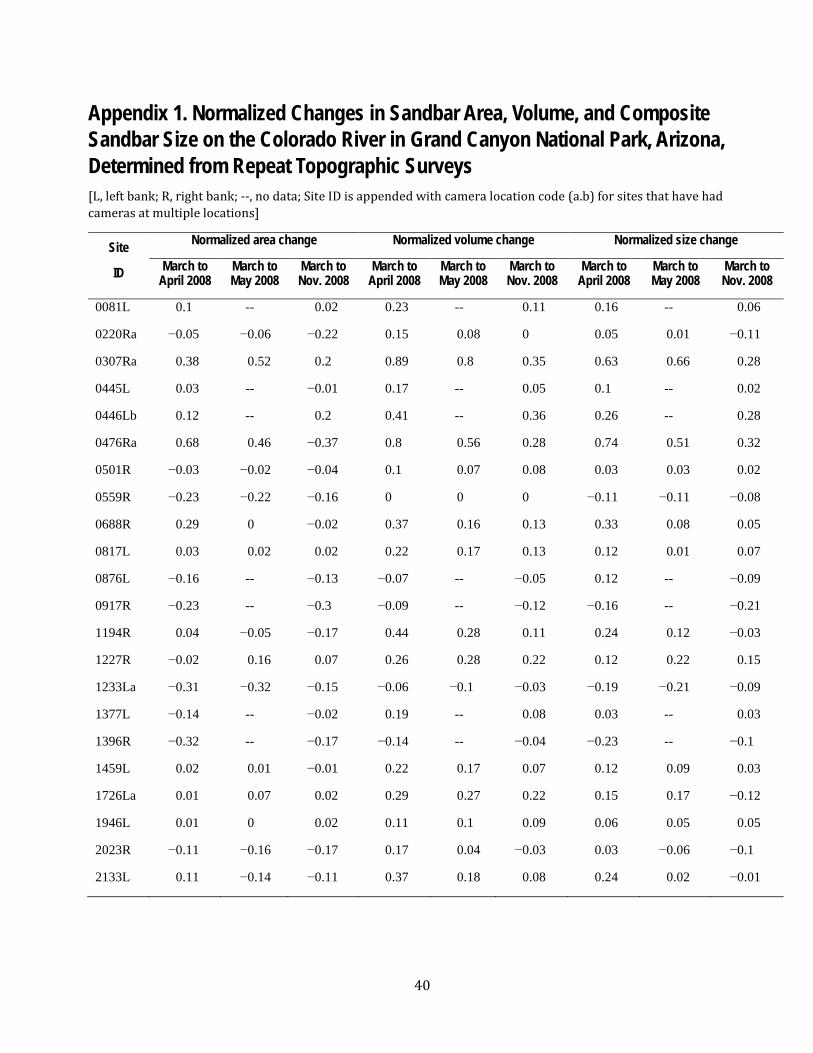
40
Appendix 1. Normalized Changes in Sandbar Area, Volume, and Composite Sandbar Size on the Colorado River in Grand Canyon National Park, Arizona, Determined from Repeat Topographic Surveys [L, left bank; R, right bank; --, no data; Site ID is appended with camera location code (a.b) for sites that have had cameras at multiple locations]
Site
ID
Normalized area change Normalized volume change Normalized size change
March to April 2008
March to May 2008
March to Nov. 2008
March to April 2008
March to May 2008
March to Nov. 2008
March to April 2008
March to May 2008
March to Nov. 2008
0081L 0.1 -- 0.02 0.23 -- 0.11 0.16 -- 0.06
0220Ra −0.05 −0.06 −0.22 0.15 0.08 0 0.05 0.01 −0.11
0307Ra 0.38 0.52 0.2 0.89 0.8 0.35 0.63 0.66 0.28
0445L 0.03 -- −0.01 0.17 -- 0.05 0.1 -- 0.02
0446Lb 0.12 -- 0.2 0.41 -- 0.36 0.26 -- 0.28
0476Ra 0.68 0.46 −0.37 0.8 0.56 0.28 0.74 0.51 0.32
0501R −0.03 −0.02 −0.04 0.1 0.07 0.08 0.03 0.03 0.02
0559R −0.23 −0.22 −0.16 0 0 0 −0.11 −0.11 −0.08
0688R 0.29 0 −0.02 0.37 0.16 0.13 0.33 0.08 0.05
0817L 0.03 0.02 0.02 0.22 0.17 0.13 0.12 0.01 0.07
0876L −0.16 -- −0.13 −0.07 -- −0.05 0.12 -- −0.09
0917R −0.23 -- −0.3 −0.09 -- −0.12 −0.16 -- −0.21
1194R 0.04 −0.05 −0.17 0.44 0.28 0.11 0.24 0.12 −0.03
1227R −0.02 0.16 0.07 0.26 0.28 0.22 0.12 0.22 0.15
1233La −0.31 −0.32 −0.15 −0.06 −0.1 −0.03 −0.19 −0.21 −0.09
1377L −0.14 -- −0.02 0.19 -- 0.08 0.03 -- 0.03
1396R −0.32 -- −0.17 −0.14 -- −0.04 −0.23 -- −0.1
1459L 0.02 0.01 −0.01 0.22 0.17 0.07 0.12 0.09 0.03
1726La 0.01 0.07 0.02 0.29 0.27 0.22 0.15 0.17 −0.12
1946L 0.01 0 0.02 0.11 0.1 0.09 0.06 0.05 0.05
2023R −0.11 −0.16 −0.17 0.17 0.04 −0.03 0.03 −0.06 −0.1
2133L 0.11 −0.14 −0.11 0.37 0.18 0.08 0.24 0.02 −0.01

41
Appendix 2. Estimated Changes in sandbar size on the Colorado River in Grand Canyon National Park, Arizona, from Remote-Camera Images for the 2012, 2013, 2014, and 2016 Controlled Floods Released from Glen Canyon Dam
[L, left bank; R, right bank; --, no data]
Site ID November 2012 controlled flood
Preflood to late Nov. 2012
Preflood to Feb. 2013
Preflood to May 2013
Preflood to Nov. 2013
0025L 1 0 0 0
0081L 1 0 0 0
0089L 1 0 0 0
0166L 0 0 0 0
0220R 2 0 0 1
0307R 1 1 1 1
0319R 1 1 0 0
0414R 0 1 1 1
0434L 0 0 0 0
0445L 0 0 0 0
0450L 2 1 1 1
0476R 0 −1 −1 −1
0501R 0 0 0 0
0515L −1 0 0 0
0559R 0 0 0 0
0651R 2 1 1 −1
0658L 0 0 0 1
0661L 1 0 1 1
0688R 1 1 1 0
0817L 1 0 0 0
0876L 0 −1 −1 0
0917R −1 −1 −1 0
0938L 1 1 1 0
1044R 1 1 0 0
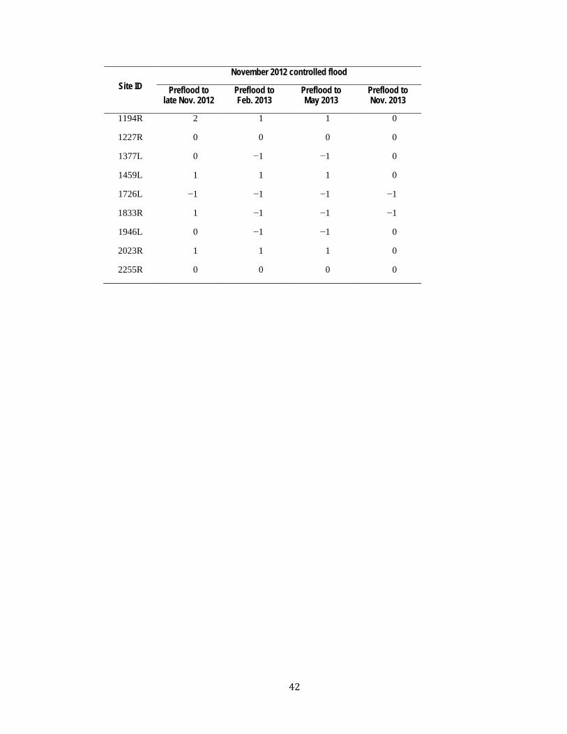
42
Site ID November 2012 controlled flood
Preflood to late Nov. 2012
Preflood to Feb. 2013
Preflood to May 2013
Preflood to Nov. 2013
1194R 2 1 1 0
1227R 0 0 0 0
1377L 0 −1 −1 0
1459L 1 1 1 0
1726L −1 −1 −1 −1
1833R 1 −1 −1 −1
1946L 0 −1 −1 0
2023R 1 1 1 0
2255R 0 0 0 0
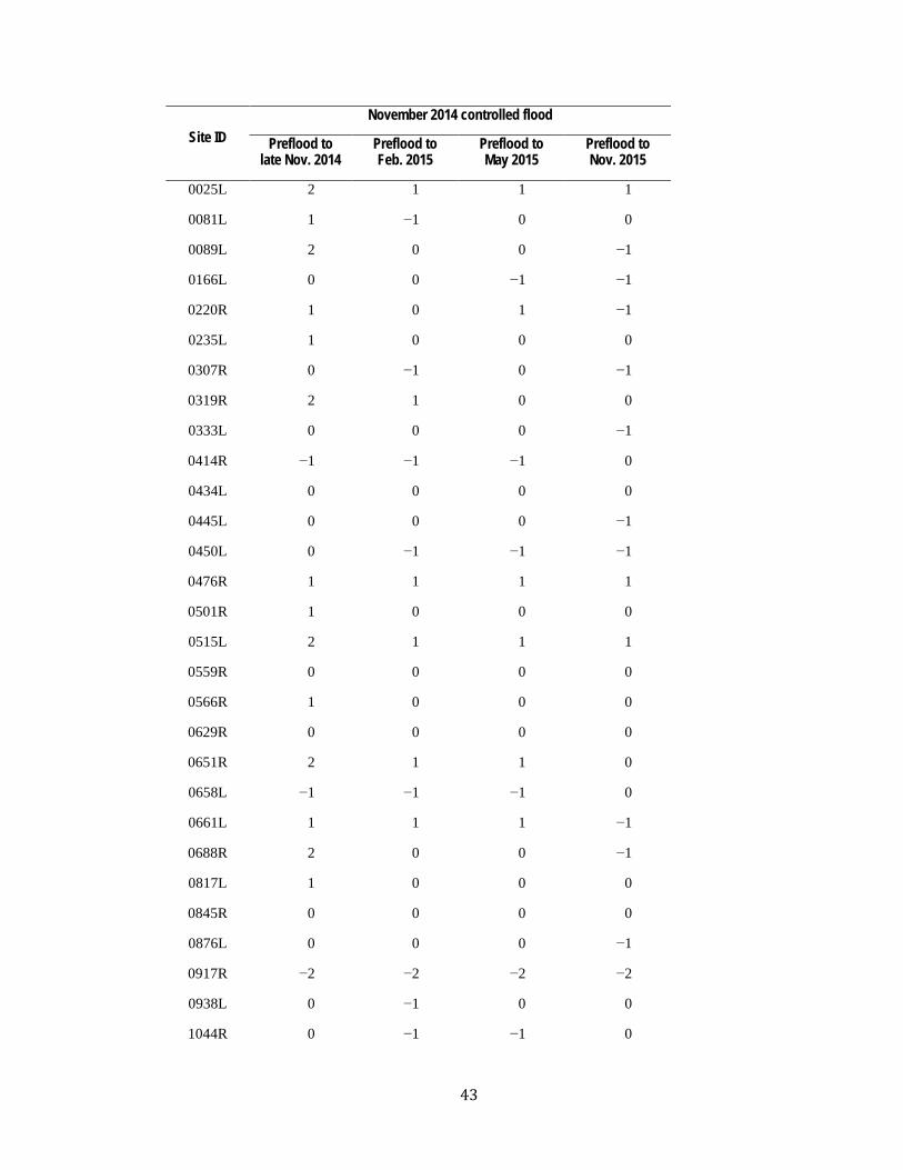
43
Site ID November 2014 controlled flood
Preflood to late Nov. 2014
Preflood to Feb. 2015
Preflood to May 2015
Preflood to Nov. 2015
0025L 2 1 1 1
0081L 1 −1 0 0
0089L 2 0 0 −1
0166L 0 0 −1 −1
0220R 1 0 1 −1
0235L 1 0 0 0
0307R 0 −1 0 −1
0319R 2 1 0 0
0333L 0 0 0 −1
0414R −1 −1 −1 0
0434L 0 0 0 0
0445L 0 0 0 −1
0450L 0 −1 −1 −1
0476R 1 1 1 1
0501R 1 0 0 0
0515L 2 1 1 1
0559R 0 0 0 0
0566R 1 0 0 0
0629R 0 0 0 0
0651R 2 1 1 0
0658L −1 −1 −1 0
0661L 1 1 1 −1
0688R 2 0 0 −1
0817L 1 0 0 0
0845R 0 0 0 0
0876L 0 0 0 −1
0917R −2 −2 −2 −2
0938L 0 −1 0 0
1044R 0 −1 −1 0

44
Site ID November 2014 controlled flood
Preflood to late Nov. 2014
Preflood to Feb. 2015
Preflood to May 2015
Preflood to Nov. 2015
1194R 2 1 1 0
1227R 1 1 1 0
1232L −1 −2 −2 −1
1377L −1 −1 0 −1
1459L 1 0 0 0
1671L 1 1 1 −1
1726L 1 1 1 0
1833R 1 −1 −1 −1
1946L 1 0 −1 −1
2023R 2 1 1 0
2132L 0 0 0 0
2201L 0 0 0 0
2255R 0 0 0 0

45
Site ID November 2014 controlled flood
Preflood to late Nov. 2014
Preflood to Feb. 2015
Preflood to May 2015
Preflood to Aug. 2015
Preflood to Sept. 2015
0025L 1 0 −1 0 0
0081L 1 1 1 0 0
0089L 0 0 0 −1 −1
0166L 1 1 1 0 0
0220R 0 0 0 0 0
0235L 2 1 1 1 0
0307R 1 1 0 0 −1
0319R 1 0 0 0 0
0333L −1 −1 −1 −1 −1
0414R −1 −1 −1 −1 −1
0434L 0 0 0 0 0
0445L 0 0 −1 −1 −1
0450L 1 0 −1 0 0
0476R 2 -- -- -- 0
0501R 0 −1 −1 −1 1
0515L −1 −1 −2 −2 −2
0559R 1 1 1 1 0
0566R 2 1 0 0 0
0629R 1 1 1 1 0
0651R 1 -- -- -- 0
0658L −2 −2 −2 −2 −2
0661L 2 1 1 0 0
0688R 1 0 0 0 0
0817L 1 0 0 0 0
0845R 1 0 −1 0 −1
0876L 0 0 0 0 --
0917R 0 −1 −1 −1 −1
0938L 0 0 0 0 0
1044R 1 0 0 0 0
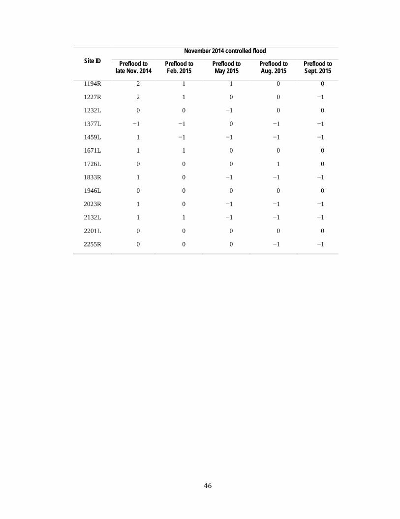
46
Site ID November 2014 controlled flood
Preflood to late Nov. 2014
Preflood to Feb. 2015
Preflood to May 2015
Preflood to Aug. 2015
Preflood to Sept. 2015
1194R 2 1 1 0 0
1227R 2 1 0 0 −1
1232L 0 0 −1 0 0
1377L −1 −1 0 −1 −1
1459L 1 −1 −1 −1 −1
1671L 1 1 0 0 0
1726L 0 0 0 1 0
1833R 1 0 −1 −1 −1
1946L 0 0 0 0 0
2023R 1 0 −1 −1 −1
2132L 1 1 −1 −1 −1
2201L 0 0 0 0 0
2255R 0 0 0 −1 −1
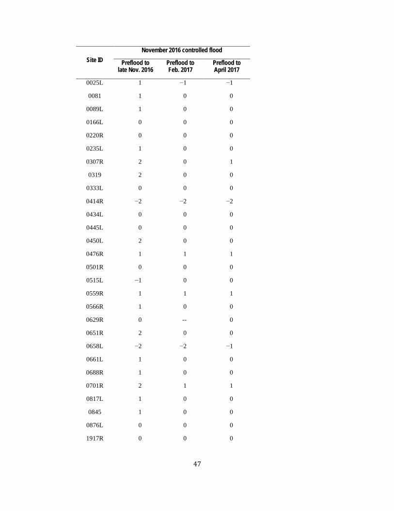
47
Site ID November 2016 controlled flood
Preflood to late Nov. 2016
Preflood to Feb. 2017
Preflood to April 2017
0025L 1 −1 −1
0081 1 0 0
0089L 1 0 0
0166L 0 0 0
0220R 0 0 0
0235L 1 0 0
0307R 2 0 1
0319 2 0 0
0333L 0 0 0
0414R −2 −2 −2
0434L 0 0 0
0445L 0 0 0
0450L 2 0 0
0476R 1 1 1
0501R 0 0 0
0515L −1 0 0
0559R 1 1 1
0566R 1 0 0
0629R 0 -- 0
0651R 2 0 0
0658L −2 −2 −1
0661L 1 0 0
0688R 1 0 0
0701R 2 1 1
0817L 1 0 0
0845 1 0 0
0876L 0 0 0
1917R 0 0 0

48
Site ID November 2016 controlled flood
Preflood to late Nov. 2016
Preflood to Feb. 2017
Preflood to April 2017
0938L 1 0 0
1044R 0 -- --
1194R 2 1 1
1227R 0 0 0
1232L 1 1 1
1377L −1 0 0
1459L 1 0 0
1671L 1 1 0
1726L 0 0 0
1833R 1 0 0
1946L −1 −1 −1
2023R 0 0 0
2132L 1 0 0
2201L 0 0 0
2255R 1 0 0
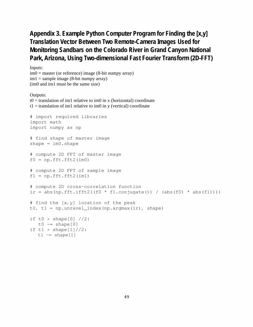
49
Appendix 3. Example Python Computer Program for Finding the [x,y] Translation Vector Between Two Remote-Camera Images Used for Monitoring Sandbars on the Colorado River in Grand Canyon National Park, Arizona, Using Two-dimensional Fast Fourier Transform (2D-FFT) Inputs: im0 = master (or reference) image (8-bit numpy array) im1 = sample image (8-bit numpy array) (im0 and im1 must be the same size) Outputs: t0 = translation of im1 relative to im0 in x (horizontal) coordinate t1 = translation of im1 relative to im0 in y (vertical) coordinate # import required libraries import math import numpy as np # find shape of master image shape = im0.shape # compute 2D FFT of master image f0 = np.fft.fft2(im0) # compute 2D FFT of sample image f1 = np.fft.fft2(im1) # compute 2D cross-correlation function ir = abs(np.fft.ifft2((f0 * f1.conjugate()) / (abs(f0) * abs(f1)))) # find the [x,y] location of the peak t0, t1 = np.unravel_index(np.argmax(ir), shape) if t0 > shape[0] //2: t0 -= shape[0] if t1 > shape[1]//2: t1 -= shape[1]

50
Appendix 4. Example Python Computer Program for Finding the Area of a Polygon in Projected [x,y] Coordinates Inputs: x = polygon coordinates in x direction (Easting, m) y = polygon coordinates in y direction (Northing, m) Outputs: a = area in m2 # import required libraries import numpy as np # compute area A = 0.5*np.abs(np.dot(x, np.roll(y,1))-np.dot(y, np.roll(x,1)))