i

Group Members:

Douglas Cooper Desmond Persaud

Samael Reyna

August 10, 2009

Group 4

Automated Plant

Growth System

ii

This page has been intentionally left blank.

iii

Table of Contents EXECUTIVE SUMMARY ........................................................................................................................... 1

MOTIVATION .............................................................................................................................................. 1

CHAPTER 1: PROJECT IDENTIFICATION .......................................................................................... 2

1.1 INTRODUCTION ....................................................................................................................................... 2 1.2 REQUIREMENTS ...................................................................................................................................... 3

1.2.1 General ........................................................................................................................................... 3 1.2.2 Lighting System .............................................................................................................................. 4 1.2.3 Sensors ........................................................................................................................................... 4 1.2.4 Regulation ...................................................................................................................................... 5 1.2.5 System Interface ............................................................................................................................. 5 1.2.6 Structure ......................................................................................................................................... 5 1.2.7 Power System ................................................................................................................................. 5

1.3 SPECIFICATIONS ..................................................................................................................................... 5

CHAPTER 2: SENSORS .............................................................................................................................. 7

2.1 PH SENSOR ............................................................................................................................................. 7 2.2 TEMPERATURE SENSOR ........................................................................................................................ 10 2.3 HUMIDITY SENSOR ............................................................................................................................... 11 2.4 LIQUID LEVEL SENSOR ......................................................................................................................... 17 2.5 CARBON DIOXIDE (CO2) SENSOR ......................................................................................................... 23 2.6 NUTRIENT SENSOR ............................................................................................................................... 26

CHAPTER 3: SYSTEM INTERFACE AND CONTROLS .................................................................... 28

3.1 MICROCONTROLLERS ........................................................................................................................... 28 3.2 NETWORKING ....................................................................................................................................... 33 3.3 SOFTWARE USER INTERFACE ............................................................................................................... 36

CHAPTER 4: REGULATION ................................................................................................................... 37

4.1 LIGHTING SYSTEM ................................................................................................................................ 37 4.1.1 Light Source ................................................................................................................................. 37 4.1.2 Adjustment .................................................................................................................................... 39 4.1.3 Motor ............................................................................................................................................ 43 4.1.4 Optical Sensor .............................................................................................................................. 48 4.1.5 Contact Sensor ............................................................................................................................. 51

4.2 FEEDING SYSTEM ................................................................................................................................. 54 4.2.1 pH and Nutrients .......................................................................................................................... 54 4.2.2 Feeding Pump............................................................................................................................... 62 4.2.3 Mixing........................................................................................................................................... 63

CHAPTER 5: POWER SYSTEM .............................................................................................................. 67

5.1 AC/DC AND AC/AC CONVERSION ...................................................................................................... 67 5.2 POWER DISTRIBUTION AND BUS .......................................................................................................... 69 5.3 RELAYS ................................................................................................................................................ 69

CHAPTER 6: STRUCTURE ..................................................................................................................... 71

6.1 STRUCTURE METHODS ......................................................................................................................... 71 6.2 SENSORS ............................................................................................................................................... 75 6.3 LIGHTING ............................................................................................................................................. 77 6.4 FRAME AND ELECTRONICS PROTECTION .............................................................................................. 77 6.5 PIPING .................................................................................................................................................. 77 6.6 RESERVOIRS ......................................................................................................................................... 78

iv

CHAPTER 7: BUILD ................................................................................................................................. 80

7.1 GROUP RESPONSIBILITIES .................................................................................................................... 80 7.2 PROJECT SCHEDULE ............................................................................................................................. 80 7.3 BILL OF MATERIALS ............................................................................................................................ 82 7.4 BUDGET AND FINANCING .................................................................................................................... 84 7.5 DESIGN SUMMARY .............................................................................................................................. 84

CHAPTER 8: TESTING ............................................................................................................................ 99

8.1 FACILITIES AND EQUIPMENT ................................................................................................................ 99 8.2 TESTING PROCEDURES ......................................................................................................................... 99

8.2.1 Sensors ......................................................................................................................................... 99 8.2.2 Lighting ...................................................................................................................................... 100 8.2.3 Pumps and Valves ...................................................................................................................... 100 8.2.4 Power System ............................................................................................................................. 101

SUMMARY AND CONCLUSIONS ....................................................................................................... 101

APPENDICES (See Attached CD)

A. Copyright Permissions B. Data Sheets

1

Executive Summary The main idea of this project is characterized by the ability to automatically measure and regulates the main growth characteristics of plants while requiring minimal user interaction. Some of the controllable features in this project include regulation of nutrient concentration and pH level of our solution. This system also gives feedback of CO2 level, humidity, temperature and liquid level of our mixture. A valve and pump system is used for water regulation and draining, which includes a liquid level pressure sensor and a feeding pump. An automated lighting level adjustment is also integrated into the project. A wireless interface hosted by a web-server offers a web-based GUI for system settings and viewing of environmental conditions. Most of these controls for the project are based on the data that is taken from the sensors that we have selected. For the sensors in the project, we used specific meters that detect the level of that given solution. Most of these sensors have analog outputs must be adjusted to a proper interval for the A/D converters so that microcontrollers can do the calculations and output different information to the web with the wireless controller which is displayed on the web page online. The frame is a rigid wood structure because of the strength and low cost that it gives us. A web interface allows the user to access the system easily from anywhere on the planet. This allows the user the ability to monitor almost all elements and regulate certain portions of the simulated environmental conditions of a specific plant in the system.

Motivation The overall motivation of this project originated from two main ideas: the concern of food consumption with rising populations given scarce environmental and spatial resources and the future of space exploration and colonization on the moon and other planets. As time progresses, the availability of farm land will slowly diminish as more urban developments are needed to accommodate the growth of a rising world population which may potentially leave society with limited options to produce food for a given community. Additionally, if mankind wishes to survive in environments where natural growth is not possible, methods must be developed in order to sustain a livable environment. In response to these movements, many researchers have begun to develop alternatives to traditional growth methods. One major method is to construct in-door growing facilities that can eliminate the need for large areas of land by utilizing multiple story buildings with environments that regulate the necessary conditions for plants to strive. Not only can this method be applied here on earth but elsewhere as well.

2

Chapter 1: Project Identification

1.1 Introduction This Automated Plant Growth System utilizes a hydroponic environment which offers a solution to automatically monitor and regulate some of the basic and critical elements that optimizes growth of plants, as well as provides feedback for some of the conditions surrounding the plant. The portion of the system that is regulated includes nutrient consumption and artificial lighting while the feedback portion is provided for Carbon Dioxide level, humidity and temperature. For effective nutrient consumption to take place, two things must be monitored: the conductivity and pH levels of the growth medium which is measured through the use of specialized probes. Once effective measurements are processed by the system, peristaltic-type pumps allows for precise dispensing of the needed chemicals in order to stabilize the growth environment. The main chemicals incorporated in this project are a general nutrient solution which is used in hydroponics cultivation as well as pH Up/Down solutions which are essential for effective nutrient absorption by the plant. Because it is necessary to keep the growth environment periodically clean and fresh, a pump and valve system must be incorporated that allows for two different configurations. The first configuration is through the use of large containers, one of which is used to source the clean water and the other which is used to drain the old solution. In this case, both bins can either be used in a gravity or pump based pressurized system. This setup would require that the user periodically fill and drain the containers which can be somewhat cumbersome but yet may be a desirable option. The second configuration allows the user to connect a pressurized water system, such as municipal city water, as well as a drainage piping in order to reduce the amount of user interaction with the system. For demonstration purposes the first of the two configurations is the desirable option. In order to keep track of the solution level inside the growth medium a pressure sensor is utilized. An additional pump has been added to the system that is placed inside the growth solution. This pump allows for the user to have two separate feeding options. The default option allows the user to set the solution level so that the roots of the plants are constantly submerged inside the solution, which is commonly known as a “deep water culture” method. The second option which utilizes the pump, allows for a modified “wicking” method where tubing is routed up the center of the feeder and over the plants which gives the user the option to set timed feedings. Additionally, a combination of both methods can be implemented simultaneously. The main goal here is to provide variability as all plants may not grow the same under one set of conditions As lighting is the one of the most critical elements needed for plant growth much consideration has been made on how to approach this part of this system. In lieu

3

of the “going green” idea, it was chosen that the lighting be LED based which uses much less power and last longer than typical indoor grow lights. The downfall to using these types of source is that they do not provide as much intensity as the traditional sources. On the plus side, however, because LED lighting does not emanate with nearly as much heat as the traditional lighting sources, they can be placed much closer to the plants. With this idea in mind, the basis of the lighting system allows for the light to maintain a constant distance from the plant and self adjust as the plant grows utilized special sensor and a motor/pulley system to accomplish this. One additional feature that the light system offers is day and night cycling to simulate a typical environment. In order to minimize user interaction, a wireless interface is incorporated that can allow a user to locally interact with the system in an “ad-hoc” or local network as well as through the internet. This is accomplished by an on-board wireless server that hosts a web page which acts as a GUI type user interface allowing the user to view the various conditions of the system as well as setup configuration the settings of the system. The main idea behind the wireless feature is to show that on a grander scale, arrays of these feeders can be configured on a single network and controlled from anywhere. The controlling PC need not even have any localized software, just an internet connection. However, the local network in which the growth system is hosted should have a sizeable router for the feeders to connect to. The web page itself is a simple, easy to use interface that allows the user to not configure the system but view data logged information that characterizes the life of the plant over a given period of time. Additionally, the on-board server hosts a database which contains two types of information. The first is a general database of common growth characteristics of various plant types so that a user may easily set up the system without a lot of knowledge of the plants that are being grown. Of course the more knowledgeable users have the ability to define specific settings and add to the database if they so choose to.. 1.2 Requirements These requirements were developed from the engineer’s initial meetings and decisions on how the system should be built. After careful consideration and discussion, this set of requirements has been created as a guide for the engineers to follow while doing research on their selected topics. 1.2.1 General

• The system shall utilize a soilless, hydroponic environment. • The general size of the system is designed for small plants such as herbs

and sunflowers. This was decided on because if you try to grow large plants in the system, it becomes very difficult to transport or to monitor because of the large changes that the system can have through the course of a given day. The plants is ideal if they stay within two feet because of the height of our lighting system

4

1.2.2 Lighting System

• The lighting shall utilize an LED setup suitable for plant growth given the size of the structure. The light weight and low power of a square foot LED lighting board gives us the necessary light for the small plants in the system.

• The lighting shall be implemented such that the light source automatically adjusts as the plant grows. Should the plant reach the given height, it would be best if the plant moves automatically vertical as to not obstruct the plants growth.

• There shall be an optical sensor such that the maximum height of the plant is detected. Again, this is to not obstruct the growth of the plant and allow it to grow to its full potential.

• There shall be a contact sensor such that the lighting system has a reference point for proper adjustment. This requirement is here because our lighting system is at a maximum height of two feet and so it is known when we have reached this limit.

1.2.3 Sensors

• The system shall have a sensor which measures the pH level of the feeding solution. If the pH is not carefully registered and monitored, the plant could start to have many adverse effects. This sensor will also allow us to input chemical solutions which will change the pH based on the point of pH per quarter tablespoon that is needed.

• The system shall have a sensor which measures the nutrient content of the feeding solution. This is necessary because you need to know when you have a solution that is either to high of a concentration or when the solution does not have high enough concentration. The plant will require different values of nutrient input during different stages of its life. These values are shown in table 4.2.1.1

• The system shall have a sensor which measures solution level. This is needed because with the level of liquid known, we can mix the correct parts per million of the nutrient and pH chemical solution input.

• The system shall have a sensor which measures Temperature. The temperature sensor is input into the system so that parts of the simulated environment can be monitored.

• The system shall have a sensor which measures Humidity. Like the temperature sensor, this is input into the system because of the need to monitor the environmental conditions of the plant to note any relation between the change in pH or any diseases or fungus that can be contracted by the plant.

• The system shall have a sensor which measures the CO2 level in its surroundings. As the two sensors above, this is to measure additional environmental conditions.

5

1.2.4 Regulation

• The system shall be able to regulate the pH level of the feeding solution. This regulation is useful to the user because you can simulate optimum growing conditions if they so desire.

• The system shall be able to regulate the nutrient level of the feeding solution. At different growing stages, the plant can receive the required nutrient level but the pH can have a change in the way the plant absorbs nutrients.

• The system shall be able to regulate the solution level of the feeding solution. If the user desires to add addition plants or remove certain plants from the system, there should be a way to change the liquid level by either opening input valves or exit valves.

• The system shall be able to regulate day and night lighting cycles. If the ability to regulate day and night is granted to the user, the user has the potential to simulate similar results as in some northern states.

1.2.5 System Interface

• The system shall implement a web-based interface for user interaction. This will give almost full control from anywhere that internet is available.

• The system shall utilize an onboard data server with the capability of hosting a web interface. The interface shall provide the following features:

o Real time display of all measurements o Provide daily time lapsed photos of plant o Predefined database and user defined growth characteristics o Data log of plant growth history

1.2.6 Structure

• The structure is a solid wooden frame what can hold the weight of all the electrical components and a 15 gallon solution. The combined weight should be enough to hold 150 lbs to support all the water and the electrical components.

1.2.7 Power System

• Provide AC to DC conversion that will give a maximum of 50 voltages. This is not a final value but the high enough voltage so that it can be divided into reasonable ranges per unit required. Also an AC to AC converter for the smaller objects that need smaller ac voltage.

1.3 Specifications

The size of the structure shall be such that four small plants is able to occupy the space. The products selected to be used in the system have

6

enough power to handle the amount of plants as long as they are not of larger variety.

• General dimensions of the structure should be at a minimum of 18x14x14 inches. These measurements were selected because of the power that our system can generate and what our systems products limitations are.

• The pots in which hold the plants are held should be between 2 and 3 inches. This size of pot allows a decent sized plant in the system and keeps the plant in a specific size and range.

• The pots should be evenly spaced in a square-like fashion with a separation of at least 3 inches. This makes it so that the feeding pump has enough pressure to push the solution upward and distribute the solution evenly.

• The structure shall allow for a maximum of fifteen gallons and a minimum of 0 gallons. At a maximum level the liquid should be just shy of spilling out of the container. It should be filled to about seventy five percent of the total size so that the re-entry process spills as little as possible. The pressure specifications and the flow input are also matched to this level.

• The Humidity sensor shall allow for a range of 0 to 100% RH and a precision of 3% RH. This is the specifications given off of the sensor selected. While it can read a wide range of values, there only a specific range that we would be using.

• The temperature sensor shall allow for a range of 0 to 85o C with a precision of 1oC. Most of the chemical solutions and the products themselves require a relatively low temperature to function correctly. This is actually a good set limit to make sure that the system is still within reasonable operating temperature and gives a flag as to when the user should adjust any parameters.

• The liquid level sensor should have a minimum range of 0 to 21.5 cm with accuracy of .5 cm. This is going to be well within a reasonable range of accuracy because the changes within that scale is acceptable because that low of a change of liquid level will not have too large of an impact on the system.

• The pH sensor should read from 0 to 14 on a pH scale with an accuracy of 1 pH. This is not completely needed, but it is nice to be able to track such drastic changes. The normal range of the pH should stay around 5.5 with a one level increase or decrease as described in the design consideration of section 2.1

• The Carbon dioxide sensor shall allow for a range of 0 – 2500 ppm and a precision of 10 ppm.

• The day and night light cycles allows for a minimum day conditions of 8 hours during each cycle. While we can have it up to 24 hours a day, we would like to make it such that the plant has no less than 8 hours a cycle because any less may start to stun the plants growth or have other negative side effects.

7

Chapter 2: Sensors

2.1 pH Sensor Introduction When trying to keep a well balanced chemical solution it is wise to keep pH levels regulated. If its pools, fish tanks, or a plants chemical solution, the wrong pH level has the potential of harming the host. For a mixture over 50 gallons it is recommended to check the levels about once a day. For smaller systems it is not critical to check the solution so often. Usually plants grown in hydroponic systems tend to stay around the same pH levels pending plants roots growing a fungus which can drastically change the pH levels. Design Considerations Regardless of what pH you have, it’s almost always a system which has two contacts that are in close proximity. These contacts have a send and receive node which test changes that occur in the space between which is used to calculate conductivity. While there is a very small order of conductivity in pure water, the impurities that the nutrient solution and the plant add to the water are enough to get a useful pH value. It is recommended that whatever product is decided on, it should be waterproof. The cost goes down with the products that are not submersible but they also tend to break quicker. A meter in our system should by small and lightweight in size. There are a couple critical things to note as far as pH is concerned and below is information that was taken directly from TPS.com in the hydroponic section dealing with pH effects:

• pH can affect the availability of nutrients. • pH can affect the absorption of nutrients by plant roots • pH values above 7.5 cause iron, manganese, copper, zinc and boron ions

to be less available to plants. • pH values below 6 cause the solubility of phosphoric acid, calcium and

magnesium to drop. • pH values between 3 and 5 and temperatures above 26°C encourage the

development of fungal diseases1 Fiber Optic pH Sensors The Fiber Optic pH Sensor system consists of a fiber optic probe designed to hold immobilized colorimetric indicator dye materials, plus a light source, spectrometer and OOISensors Software. You can supply your own indicator material, or select from our line of transparent or reflective films. Calibration

1 http://www.tps.com.au/hydroponics/pheffect.htm

8

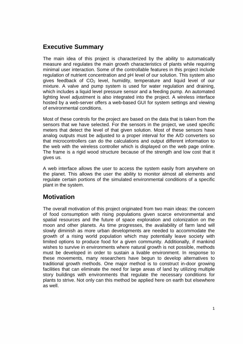
involves recording spectra in high and low pH samples, and in at least one pH standard such as a NIST-traceable buffer. Electrode Sensors Most of the common handheld sensors that are on the market are electrode based, possibly because of their simplicity. It has a reference point which is usually calibrated then two contacts at the end of the electrode which capture measurements of pH by passing voltage from one side to the other. Device Selection One of the two final devices that the group has decided on has been the Hanna instrument Checker 1 listed below as figure 2.1.1 which list pH range from 0.00 to 14.00. While it is nice to have a complete range of possible values, it should be noted that anything past certain limits is irrelevant because of the fact that the plant cannot survive in those conditions. One positive to having all the possible values tracked is the ability to check against other data showing possible signs which could have lead to the change in the pH of the solution. The solution should stay between a level of five and seven. Above in the bulleted list it shows a list of different values of pH and what effect they have on the plant. It should be programmed into the microcontroller as to when it should try to adjust the plants pH balance based on life cycle. The listed accuracy of the unit is +/- 0.2. This is useful because it is not as critical to get more precision than that. Once the pH is a full point away from the needed value is the time which adjusting should be considered. One thing to keep in mind is the fact that it takes time for the pH to change from the normal factors like temperature and the plant itself, but also when the pH solution is added to the system. Changing the pH with a chemical solution has to compensate for the time it takes the pumps to input the liquid into the solution and also for the pumps to thoroughly mix the chemical input. They have listed that the resolution is 0.01. This is also well in the desirable range because it only has to be at levels that are a half or full point away from the desired pH levels which causes negative effects to the plant. The pH is calibrated manually through two points through trimmers. The unit itself does require batteries, two 1.5v batteries that last approximately three thousand hours of continuous use. The unit is desired to be on for an indefinite amount of time and the current intentions are to regulate the voltage going in so that the correct voltage is supplied to the correct locations for a simulated infinite amount of time. Its temperature limitations are listed at zero to fifty degrees °C and maximum RH percentage being ninety five. This is important to the overall scheme of things and we do have the temperature and humidity sensors to capture these results. For a preset system like the one that Hanna instrument offers, it is interesting to try and tap into their system to take measurements. The product has yet to be

9

attained, so no conclusive test data can be acquired. The group has emailed the company but has received the obvious answer that data sheets or any information regarding the actual make up and components are more or less out of the question for the regular consumer. What happens in the next phase should this be the final product that is selected would be to try and carefully pull apart the unit and have it continue to run properly. The goal is to disassemble its internal components to a level small enough so that outputs can be tapped into to try and use the data in front of us. It would be easiest to get a perfect linear curve as to the outputs of the hand held probe and the connection onto the seven segment LCD display that the unit has. What is interesting to try would be to tap into the actual display of the unit and use its outputs as inputs to our microcontroller so that we can pass this data onto the internet. These components may very well be directly proportional to the actual resistance in the connections themselves and should the resistance or current be changed, even if only by a small amount, this could have very drastic changes in the output giving us unusable and could possibly ruin the product itself wasting both time and money each time that this is attempted. While it would be very interesting to try, this is a very risky approach to something that the group does not have data sheets on2.

Figure 2.1.1 with permission from Hanna Instruments Image of HI 98103 pH tester from Hanna Instruments

The second method that the group was looking into was using a probe. There are plenty of replacement probes on the market today for universal setups. The idea behind this method is that you can take a probe that is made for many products and base your circuit around these outputs. While there were large varieties out there, the one that seemed to have the easiest and widest selection of product was a BNC based connection. Most of these products all listed the same specifications. The one that was found as the most convenient because of availability and price point was a product from the VirtualVillage.com. It is unfortunate however that when looking at the product itself, it has been difficult to try and find the manufacture of this product and the only reference that was able to be located was the sku number of the product listed as 001490-008 (Figure 2.1.2). An email on our behalf has been sent to the company selling the product

2 Email directly from a gentleman by the name of Rob Samborn explicitly mentioned in an email that this

information is not open to the public, but he does commend us on our research and wishes us the best.

He writes, “any information beyond the published features and specifications is proprietary and I cannot

release it to you.”

10

and is awaiting any information regarding its origin. One the sales website they had listed some basic specifications. As many other models the instruments measurement range is the full scale from 0.00 to 14.00 pH. As mentioned above, most of these values are not used. If this meter can read the scale itself, it would be interesting to find out if it needs external software or if it is actual analogue output. This is essentially not changed from the setup above, in contrast, this is actually doing all the work for us as opposed to trying to tap into a display system where we have the large potential of possibly getting invalid data. It also goes on to list it measurement accuracy as 0.01 pH. What the desired pH levels would be only require the knowledge of the tenth decimal place, and while it is very nice to know the pH to the hundredth decimal as listed on this unit, it is not be necessary. It is undoubtedly incorporated into the microprocessors programming. The emphasis on this part is to really get a highly defined pH measurement should there be the need to track any plant habits and outputs. The BNC probe itself lists operating temperature from 0° - 50°C. At one hundred and twenty plus degr ees Fahrenheit, it would be safe to assume that you would have larger problems the pH to worry about. For the plant that the project is directed toward, these values are irrelevant, however, should we decide to build upon our maximum limits and push our growing/feeding system to grow plants that thrive in the harshest of environments, this could be very beneficial to see how to maximize these plants needs while keeping it as efficient as possible.

Figure 2.1.2 pH probe

Permission requested from VirtualVillage.com

2.2 Temperature Sensor Introduction While temperature is not a crucial variable in the plants growth and development, it can have major effects on the plants survival and yields when exposed to extreme highs or lows for lengthy periods of time. Exposure to high temperatures can cause the plants to respire at a greater rate than that of photosynthesis while exposure to low temperatures slows down the growth process meaning the plant yields less than it should. The addition of a temperature sensor into this project allows the ability to provide feedback to the system user in the event of improper conditions surrounding the plant.

11

Design Considerations Some of the major factors taken into consideration when selecting this type of component are the operating range, accuracy, response time and cost. The ideal operating temperature range should account for freezing point to greater than room temperature with an accuracy that is about 1oC and a response time that is reasonable enough to detect rapid changes in temperature. The cost should be reasonable while still allowing for a quality product that lasts a decent amount of time. The two main types of temperature sensors on the market today are the Resistance Temperature Detector (RTD) and the thermocouple which is considered in the following paragraphs. Resistance Temperature Detector (RTD) This type of resistive sensor can be made from various types of materials, all of which operate on the same underlying principle: a change in resistance is directly proportional to the change in temperature. They operate at a wide range of temperatures, are very stable and can operate under exposure to chemical environments. They are available in 2, 3 and 4 lead types where the relative accuracy increases with the number of leads. Thermocouple The basic idea of this type of sensor consists of the joining of two different metals that produce a small voltage which is proportional to the change in temperature. They operate over a wide range of temperatures and are extremely cost efficient, however they are limited by their accuracy and their increase in error with time. Component Selection It was decided that the most efficient way to implement a temperature sensor into this project would be to couple it with the Humidity sensor (Hygrometer) that is discussed in Section 2.3. System Integration See System Integration of Section 2.3. 2.3 Humidity Sensor Introduction One of the many important factors that can affect the growth of plants is Humidity. A lack or excess of humidity can play a critical role in their longevity of life as well as appearance. An excess of humidity can create an environment in which mold and other fungi are more apt to grow which causes disease to spread

12

throughout the plants. A lack of humidity dries out the plant leaving it wilted and damaged causing leaves and buds to die and fall off. To provide feedback necessary for a user to maintain proper humidity in the area of growth, a humidity sensor is included to provide accurate measurements of the plants surroundings. Design Considerations The basic definition of Humidity is the amount of water vapor found in a given quantity of air and it can be expressed in various manners which are absolute or specific humidity, a mixing ratio, vapor pressure and relative humidity. Of all of these forms, the most common method seems to be Relative Humidity (RH) which is a ratio which compares the amount of water vapor in the air to the amount that would be available if the air were saturated (or at 100% water vapor) and is measured on a scale of 0 to 100%. Since measuring relative humidity is also dependent on the temperature, many sensors of this type provide temperature measurements which make the accuracy and relative ease of implementation much better. While comparing the various methods of measurement, range, accuracy, environmental resistance, response time and cost were taken into consideration. Capacitive Sensor This type of sensor is based on the change in capacitance relative to the change in humidity, which is a result of the change in the dielectric constant of the substrate used. This type of sensor operates at a wide temperature range of up to 200oC and has a decent resistance to external chemicals, making it more than suitable to exist in the setting prescribed by this project. The maximum response time is about 1 sec for a 1% RH change and has an error of around +- 2% RH. This type of sensor also has limitations on the distance of its location from its power source. Resistive Sensor This type of sensor provides a measurement based on the change in impedance relative to the change in humidity with a value that is inversely proportional to the %RH change. The typical operating temperature ranges from -40oC to 100oC but can easily be affected by large temperature variations. These types of sensors can be easily damaged when exposed to a chemical environment. but may still be suitable if placed in a location or protected against the possible chemicals that may be used in this project. The maximum response time is about .5 sec for a 1 %RH change and has an error of around +-2%. Thermal Conductivity (Thermistor) This type of sensor measures the absolute humidity through the use if two thermistors placed in a resistive network. As current is passed through them

13

simultaneously, they begin to heat up. However, one of them is exposed to air while the other is not which allows for an uneven dissipation of heat between the two. This difference in heat leads to a difference in temperature which causes the resistivity of each to change. The difference in resistivity is directly proportional to the absolute humidity. They have the ability to operate at extremely high temperatures (>300oC) and work very well in a chemical environment. The exact response time of the sensor is unknown at this point but the precision is said to be around +-5% at lower humidity measurements with an increase in accuracy as the temperature increases. Component Selection As stated in the Temperature Sensor section, the implementation of both the Temperature and Humidity sensor is integrated into one Hydrometer type sensor. The sensor chosen for this application is a Humirel HTF3000 which provides a digital PWM signal where the output frequency is dependent on the value of the %RH. The basic specifications can be seen in the table 2.3.1 below: Description Specification Humidity Range 0 to 100% Temperature Range -40oC to 85oC Max. Supply Voltage 16 V Typical Supply Voltage 5 V Response Time 10 s

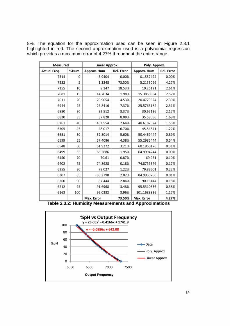
Table 2.3.1: Hygrometer Specifications 3 This device utilizes PWM as the form of measurement for the Humidity and an onboard thermistor for the temperature measurement, both of which provide the desired range of measurements. Given a 10 second response time for both outputs, it has been decided that this is not a critical element as part of the requirements and satisfies the needs of the project. System Integration It is apparent that the humidity output is connected directly to a digital input on the microcontroller since it provides a PWM signal. However, it is necessary to derive an equation for the value of %RH based on the output signal. This was done using the manufacturers collected data which is provided in Table 2.3.2. This table shows three sets of values. The first are the measured values provided by the manufacturer, while the second and third are regressions which have been made based on their values as seen in Figure 2.3.1. The first approximation is a linear regression which provides a maximum error of 73.5% below 15% RH. Above this value the maximum error is reduced to around

3 http://www.datasheetpro.com/363184_download_HTF3000_datasheet.html

14

8%. The equation for the approximation used can be seen in Figure 2.3.1 highlighted in red. The second approximation used is a polynomial regression which provides a maximum error of 4.27% throughout the entire range.

Measured Linear Approx. Poly. Approx.

Actual Freq. %Hum Approx. Hum Rel. Error Approx. Hum Rel. Error

7314 0 -5.9404 0.00% 0.1557424 0.00%

7232 5 1.3248 73.50% 5.2133056 4.27%

7155 10 8.147 18.53% 10.26121 2.61%

7081 15 14.7034 1.98% 15.3850884 2.57%

7011 20 20.9054 4.53% 20.4779524 2.39%

6944 25 26.8416 7.37% 25.5765184 2.31%

6880 30 32.512 8.37% 30.65136 2.17%

6820 35 37.828 8.08% 35.59056 1.69%

6761 40 43.0554 7.64% 40.6187524 1.55%

6705 45 48.017 6.70% 45.54841 1.22%

6651 50 52.8014 5.60% 50.4469444 0.89%

6599 55 57.4086 4.38% 55.2985444 0.54%

6548 60 61.9272 3.21% 60.1850176 0.31%

6499 65 66.2686 1.95% 64.9994244 0.00%

6450 70 70.61 0.87% 69.931 0.10%

6402 75 74.8628 0.18% 74.8755376 0.17%

6355 80 79.027 1.22% 79.82601 0.22%

6307 85 83.2798 2.02% 84.9930756 0.01%

6260 90 87.444 2.84% 90.16144 0.18%

6212 95 91.6968 3.48% 95.5510336 0.58%

6163 100 96.0382 3.96% 101.1688836 1.17%

Max. Error 73.50% Max. Error 4.27%

Table 2.3.2: Humidity Measurements and Approximatio ns

y = 2E-05x2 - 0.4166x + 1741.9

y = -0.0886x + 642.08

0

20

40

60

80

100

6000 6500 7000 7500

%pH

Output Frequency

%pH vs Output Frequency

Data

Poly. Approx

Linear Approx.

15

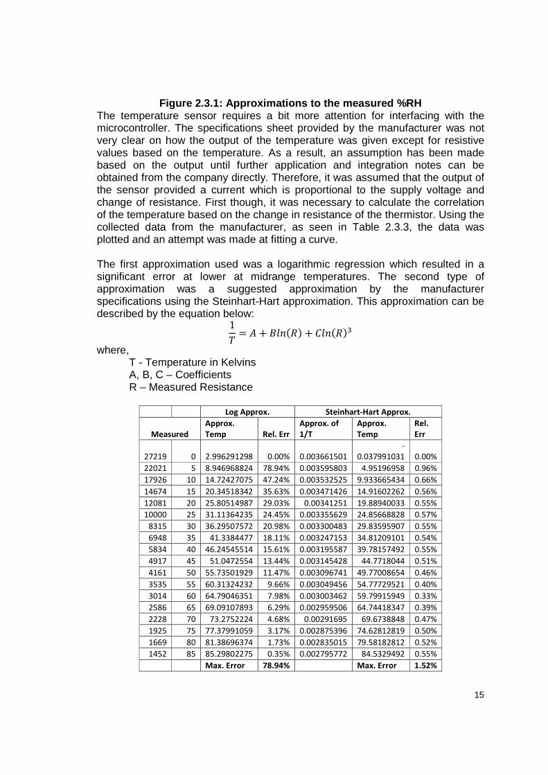
Figure 2.3.1: Approximations to the measured %RH The temperature sensor requires a bit more attention for interfacing with the microcontroller. The specifications sheet provided by the manufacturer was not very clear on how the output of the temperature was given except for resistive values based on the temperature. As a result, an assumption has been made based on the output until further application and integration notes can be obtained from the company directly. Therefore, it was assumed that the output of the sensor provided a current which is proportional to the supply voltage and change of resistance. First though, it was necessary to calculate the correlation of the temperature based on the change in resistance of the thermistor. Using the collected data from the manufacturer, as seen in Table 2.3.3, the data was plotted and an attempt was made at fitting a curve. The first approximation used was a logarithmic regression which resulted in a significant error at lower at midrange temperatures. The second type of approximation was a suggested approximation by the manufacturer specifications using the Steinhart-Hart approximation. This approximation can be described by the equation below:

1 = + +

where, T - Temperature in Kelvins A, B, C – Coefficients R – Measured Resistance

Log Approx. Steinhart-Hart Approx.

Measured

Approx.

Temp Rel. Err

Approx. of

1/T

Approx.

Temp

Rel.

Err

27219 0 2.996291298 0.00% 0.003661501

-

0.037991031 0.00%

22021 5 8.946968824 78.94% 0.003595803 4.95196958 0.96%

17926 10 14.72427075 47.24% 0.003532525 9.933665434 0.66%

14674 15 20.34518342 35.63% 0.003471426 14.91602262 0.56%

12081 20 25.80514987 29.03% 0.00341251 19.88940033 0.55%

10000 25 31.11364235 24.45% 0.003355629 24.85668828 0.57%

8315 30 36.29507572 20.98% 0.003300483 29.83595907 0.55%

6948 35 41.3384477 18.11% 0.003247153 34.81209101 0.54%

5834 40 46.24545514 15.61% 0.003195587 39.78157492 0.55%

4917 45 51.0472554 13.44% 0.003145428 44.7718044 0.51%

4161 50 55.73501929 11.47% 0.003096741 49.77008654 0.46%

3535 55 60.31324232 9.66% 0.003049456 54.77729521 0.40%

3014 60 64.79046351 7.98% 0.003003462 59.79915949 0.33%

2586 65 69.09107893 6.29% 0.002959506 64.74418347 0.39%

2228 70 73.2752224 4.68% 0.00291695 69.6738848 0.47%

1925 75 77.37991059 3.17% 0.002875396 74.62812819 0.50%

1669 80 81.38696374 1.73% 0.002835015 79.58182812 0.52%

1452 85 85.29802275 0.35% 0.002795772 84.5329492 0.55%

Max. Error 78.94% Max. Error 1.52%

16

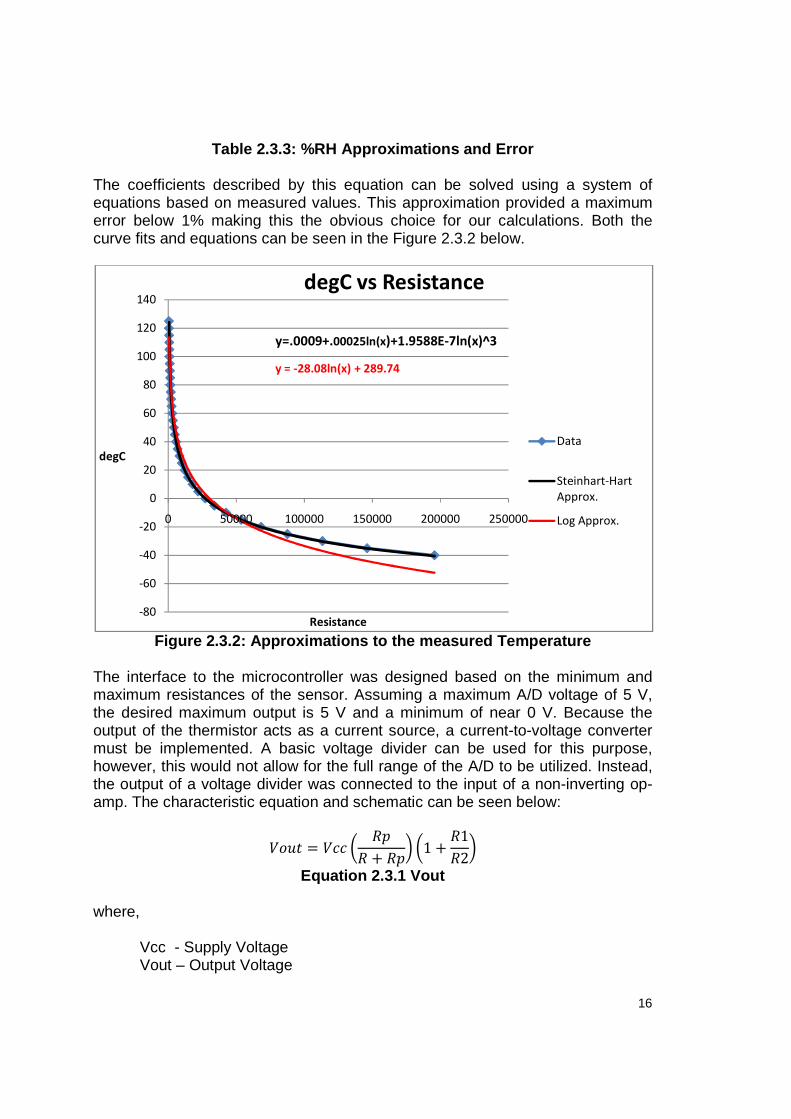
Table 2.3.3: %RH Approximations and Error The coefficients described by this equation can be solved using a system of equations based on measured values. This approximation provided a maximum error below 1% making this the obvious choice for our calculations. Both the curve fits and equations can be seen in the Figure 2.3.2 below.

Figure 2.3.2: Approximations to the measured Temper ature

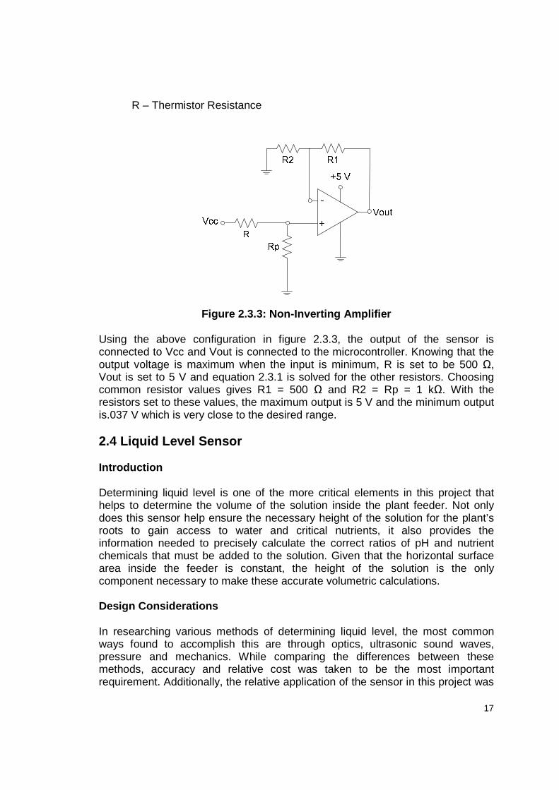
The interface to the microcontroller was designed based on the minimum and maximum resistances of the sensor. Assuming a maximum A/D voltage of 5 V, the desired maximum output is 5 V and a minimum of near 0 V. Because the output of the thermistor acts as a current source, a current-to-voltage converter must be implemented. A basic voltage divider can be used for this purpose, however, this would not allow for the full range of the A/D to be utilized. Instead, the output of a voltage divider was connected to the input of a non-inverting op-amp. The characteristic equation and schematic can be seen below:

= + 1 + 1

2

Equation 2.3.1 Vout

where,

Vcc - Supply Voltage Vout – Output Voltage

y = -28.08ln(x) + 289.74

-80

-60

-40

-20

0

20

40

60

80

100

120

140

0 50000 100000 150000 200000 250000

degC

Resistance

degC vs Resistance

Data

Steinhart-Hart

Approx.

Log Approx.

y=.0009+.00025ln(x)+1.9588E-7ln(x)^3

17

R – Thermistor Resistance

Figure 2.3.3: Non-Inverting Amplifier

Using the above configuration in figure 2.3.3, the output of the sensor is connected to Vcc and Vout is connected to the microcontroller. Knowing that the output voltage is maximum when the input is minimum, R is set to be 500 Ω, Vout is set to 5 V and equation 2.3.1 is solved for the other resistors. Choosing common resistor values gives R1 = 500 Ω and R2 = Rp = 1 kΩ. With the resistors set to these values, the maximum output is 5 V and the minimum output is.037 V which is very close to the desired range. 2.4 Liquid Level Sensor Introduction Determining liquid level is one of the more critical elements in this project that helps to determine the volume of the solution inside the plant feeder. Not only does this sensor help ensure the necessary height of the solution for the plant’s roots to gain access to water and critical nutrients, it also provides the information needed to precisely calculate the correct ratios of pH and nutrient chemicals that must be added to the solution. Given that the horizontal surface area inside the feeder is constant, the height of the solution is the only component necessary to make these accurate volumetric calculations. Design Considerations In researching various methods of determining liquid level, the most common ways found to accomplish this are through optics, ultrasonic sound waves, pressure and mechanics. While comparing the differences between these methods, accuracy and relative cost was taken to be the most important requirement. Additionally, the relative application of the sensor in this project was

18

considered based on the protection necessary for the circuitry against moisture build up inside the feeder. Optics The most common optical form of determining distance is known as Light and Distance Ranging (LIDAR). LIDAR is a method that typically comprises of a source, a detector and a reflector (the object being measured). Typically, LIDAR is accomplished using three different methods which are Electromagnetic Distance Measuring (EDM), time of flight and triangulation. The method of EDM is accomplished through the comparison of the phases of a transmitted and reflected electromagnetic wave.

Figure 2.4.1 4 Optical Distance

Permission requested from Routledge Publishing

The above diagram shows a transmitted wave being emitted at A and a wave which has been reflected from an object at B. The total distance ‘D’ can be determined by:

2 = + Δ where λm is the wavelength of the transmitted wave. Given that the phase of the transmitted wave is φ1, and that of the reflected wave is φ2 then:

Δ = [ − ]360

The only variable left to be deduced is the ‘n’ multiples of the wavelength that is repeated over the distance ‘D’. This can be accomplished by developing a system of equations by emitting two different wavelengths of light and solving for ‘n’ and then for ‘D’. This method can provide a high level of accuracy between 1 and 10 mm provided that measurement of the phase has a high resolution and

4 http://books.google.com/books?id=4eANAAAAQAAJ&printsec=frontcover#PPA163,M1

19

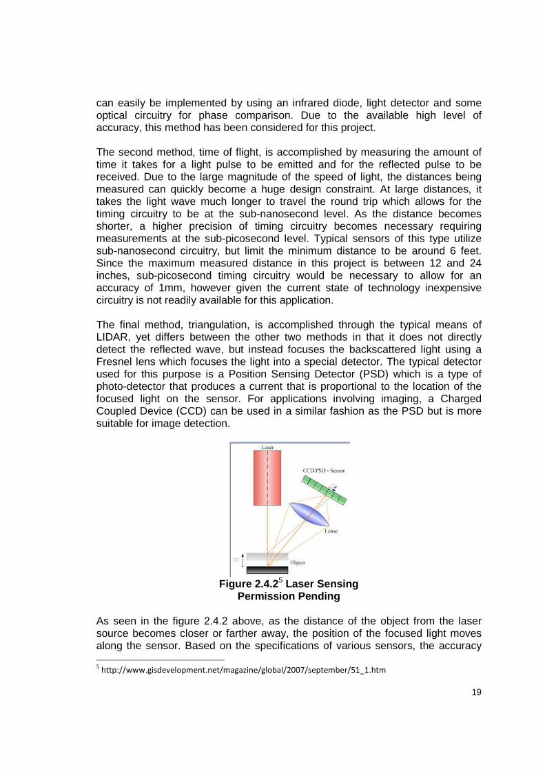
can easily be implemented by using an infrared diode, light detector and some optical circuitry for phase comparison. Due to the available high level of accuracy, this method has been considered for this project. The second method, time of flight, is accomplished by measuring the amount of time it takes for a light pulse to be emitted and for the reflected pulse to be received. Due to the large magnitude of the speed of light, the distances being measured can quickly become a huge design constraint. At large distances, it takes the light wave much longer to travel the round trip which allows for the timing circuitry to be at the sub-nanosecond level. As the distance becomes shorter, a higher precision of timing circuitry becomes necessary requiring measurements at the sub-picosecond level. Typical sensors of this type utilize sub-nanosecond circuitry, but limit the minimum distance to be around 6 feet. Since the maximum measured distance in this project is between 12 and 24 inches, sub-picosecond timing circuitry would be necessary to allow for an accuracy of 1mm, however given the current state of technology inexpensive circuitry is not readily available for this application. The final method, triangulation, is accomplished through the typical means of LIDAR, yet differs between the other two methods in that it does not directly detect the reflected wave, but instead focuses the backscattered light using a Fresnel lens which focuses the light into a special detector. The typical detector used for this purpose is a Position Sensing Detector (PSD) which is a type of photo-detector that produces a current that is proportional to the location of the focused light on the sensor. For applications involving imaging, a Charged Coupled Device (CCD) can be used in a similar fashion as the PSD but is more suitable for image detection.

Figure 2.4.2 5 Laser Sensing

Permission Pending As seen in the figure 2.4.2 above, as the distance of the object from the laser source becomes closer or farther away, the position of the focused light moves along the sensor. Based on the specifications of various sensors, the accuracy 5 http://www.gisdevelopment.net/magazine/global/2007/september/51_1.htm

20

that this method of measurement provides can be extremely precise with an error as low as .1%. The downside to this method is that it can quickly become expensive as a custom lens and a suitable laser may be required. For all methods of LIDAR, it has been noted that one of the possible pitfalls is the direct application of the electronics to moisture build up inside the feeder. In addition, any lenses used could also operate incorrectly due to the existence of moisture. Depending on possible design implementations, this type of sensor may or may not be possible. Ultrasonic Sound Waves The use of ultrasonic sound waves for the detection of distance can be accomplished by emitting a sound pulse and then measuring the amount of time it takes for the round trip similar to that of the time of flight used in LIDAR. Based on the comparison of various sensor specifications, the accuracy of this method can be less than a centimeter and in addition provides a low cost solution. One possible pitfall to this type of sensor is that it requires the emitting and sensing transducers to be directly applied inside the feeder where there is a possibility for moisture build up which could potentially ruin the circuitry. Based on tests performed by Parallax Robotics, a manufacturer of such a sensor, which placed the sensor in such conditions that would be similar to this project, it was found that the sensor continued to work after hours of application. However, a similar pitfall would be the build-up of moisture on the outside of the transducers that could prevent the transmission and/or receiving of the signal. This method has been considered as a possible solution for this project as it meets the necessary requirements. Pressure One of the more primitive forms of measurement, this method can provide a simple, accurate and cost effective solution to this project. As seen in the figure below, by connecting a tube to the end of a pressure sensor and placing the tube vertically in the solution, the sensor detects the amount of pressure inside the tube based on the water level. The basis behind this method utilizes “Hydrostatic Pressure” calculations. As the height of the liquid inside the tube changes the pressure of the liquid changes. In turn, the pressure of the air above the liquid must change to compensate for the change in liquid pressure. The following equation can be used to determine the height of the liquid:

ℎ = %&'

h - height of the liquid P - measured pressure d – density of the liquid g – force due to gravity

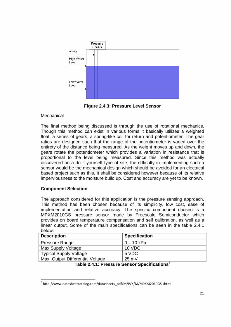
21

Figure 2.4.3: Pressure Level Sensor Mechanical The final method being discussed is through the use of rotational mechanics. Though this method can exist in various forms it basically utilizes a weighted float, a series of gears, a spring-like coil for return and potentiometer. The gear ratios are designed such that the range of the potentiometer is varied over the entirety of the distance being measured. As the weight moves up and down, the gears rotate the potentiometer which provides a variation in resistance that is proportional to the level being measured. Since this method was actually discovered on a do it yourself type of site, the difficulty in implementing such a sensor would be the mechanical design which should be avoided for an electrical based project such as this. It shall be considered however because of its relative imperviousness to the moisture build up. Cost and accuracy are yet to be known. Component Selection The approach considered for this application is the pressure sensing approach. This method has been chosen because of its simplicity, low cost, ease of implementation and relative accuracy. The specific component chosen is a MPXM2010GS pressure sensor made by Freescale Semiconductor which provides on board temperature compensation and self calibration, as well as a linear output. Some of the main specifications can be seen in the table 2.4.1 below: Description Specification

Pressure Range 0 – 10 kPa Max Supply Voltage 10 VDC Typical Supply Voltage 5 VDC Max. Output Differential Voltage 25 mV

Table 2.4.1: Pressure Sensor Specifications 6

6 http://www.datasheetcatalog.com/datasheets_pdf/M/P/X/M/MPXM2010GS.shtml

22

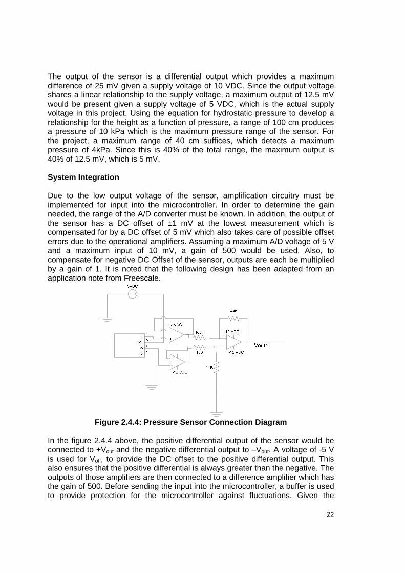
The output of the sensor is a differential output which provides a maximum difference of 25 mV given a supply voltage of 10 VDC. Since the output voltage shares a linear relationship to the supply voltage, a maximum output of 12.5 mV would be present given a supply voltage of 5 VDC, which is the actual supply voltage in this project. Using the equation for hydrostatic pressure to develop a relationship for the height as a function of pressure, a range of 100 cm produces a pressure of 10 kPa which is the maximum pressure range of the sensor. For the project, a maximum range of 40 cm suffices, which detects a maximum pressure of 4kPa. Since this is 40% of the total range, the maximum output is 40% of 12.5 mV, which is 5 mV. System Integration Due to the low output voltage of the sensor, amplification circuitry must be implemented for input into the microcontroller. In order to determine the gain needed, the range of the A/D converter must be known. In addition, the output of the sensor has a DC offset of ±1 mV at the lowest measurement which is compensated for by a DC offset of 5 mV which also takes care of possible offset errors due to the operational amplifiers. Assuming a maximum A/D voltage of 5 V and a maximum input of 10 mV, a gain of 500 would be used. Also, to compensate for negative DC Offset of the sensor, outputs are each be multiplied by a gain of 1. It is noted that the following design has been adapted from an application note from Freescale.

Figure 2.4.4: Pressure Sensor Connection Diagram

In the figure 2.4.4 above, the positive differential output of the sensor would be connected to +Vout and the negative differential output to –Vout. A voltage of -5 V is used for Voff, to provide the DC offset to the positive differential output. This also ensures that the positive differential is always greater than the negative. The outputs of those amplifiers are then connected to a difference amplifier which has the gain of 500. Before sending the input into the microcontroller, a buffer is used to provide protection for the microcontroller against fluctuations. Given the

23

minimum differential output of 0 mV and a maximum differential output of 5 mV, the resulting output of the connecting circuit is 2.5 V to 5 V. 2.5 Carbon Dioxide (CO 2) Sensor Introduction As part of the photosynthesis process, the absorption of Carbon Dioxide from a plant’s surrounding environment is critical to its survival. Through the combination of water and some added energy from sunlight, the plant produces oxygen as well as other compounds needed for survival7. To ensure that a plant exists under optimal conditions, the implementation of a Carbon Dioxide sensor can be utilized to detect various levels of this gas ranging from those levels that are beneficial to plants and humans as well as levels that indicate a contaminated environment that can be detrimental. Also, because this device is designed for indoor purposes, the sensor provides a good indication of the ventilation inside a given facility as ventilation is critical in creating conditions that mimic an outdoor environment. Though this feedback does not provide automation in this project, it does serve as an essential indicator of one of many conditions in the plant’s environment that can potentially allow for maximized growth. Design Considerations Some major considerations in the implementation of this sensor are accuracy and response time. Since the typical method for measuring CO2 levels is in parts per million (ppm), the output voltage to the device must provide a sensitivity that can produce accurate measurements with a small degree of error. For this project, the normal operating range of the sensor should be within 350 – 450 ppm which indicates normal outdoor conditions and a properly ventilated facility. The sensor should also be able to indicate much higher levels based on the fact that as the concentration of the CO2 increases the indoor air quality begins to decrease. In addition to accuracy, the ideal response time for this project should be less than one minute however it is not essential. A shorter response time would provide quicker updates to the monitoring system, however the system is configured based on the shortest allowable periods for measurement. To realize these requirements, the various forms of measurement were first considered to allow for comparison among different types of these sensors. Two major methods of measurement are through the use of Non-dispersive Infrared (NDIR) sensing and Electrolytic Cell detection. Non-dispersive Infrared (NDIR)

7 http://www.emc.maricopa.edu/faculty/farabee/BIOBK/BioBookPS.html

24

These types of sensors are comprised of an infrared source, a chamber for light, a wavelength filter and an infrared detector. Any particles trapped inside of the tube only absorb a specific wavelength of the light given off by the infrared source. The filter then allows only that particular wavelength to pass through the filter. The light intensity that is received by the detector is proportional to the number of given molecules inside the chamber and can be described through Beer’s Law8:

@ = @ABCD I = light intensity at the detector Io = light intensity of the source k = Boltzmann’s Constant P = concentration of the gas to be measured

Figure 2.5.1: NDIR Sensor Setup 9

Electrolytic Cell (EC) Detection Permission Requested from Lighttech.com

A typical sensor of this type uses a sol-gel known as NASICON and is based on the principal of “solid electrolyte”10 shown in figure 2.5.1. When the NASICON is exposed to Carbon Dioxide a chemical reaction occurs, which results in an Electro-Magnetic Force between an anode and cathode. The output voltage signal is given by Nernst’s Equation11:

E = EA − FG ln %

E = Resulting Electric field Eo = Electric field due to anode/cathode R – Universal Gas Constant T – Temperature in Kelvin z = Number of moles of electrons in reaction (in this case, 2) 8 http://www.intl-lighttech.com/applications/ndir-gas-sensors.html

9 http://www.intl-lighttech.com/applications/ndir-gas-sensors.html

10 “The MEMS Handbook”, Mohamed Gad-el-Hak, © 2002

11 http://people.clarkson.edu/~ekatz/nernst_equation.htm

25

F = Faraday’s constant P = Partial Pressure of the molecules being measured Through the research of various sensors that utilize these methods it was found that they share many common characteristics such as operating temperature and humidity range, however to meet the specifications of this project the NDIR type sensor appeared to be a more effective and accurate solution was. This type of sensor seems to provide the accuracy needed for real-time measurement, a better response time for sampling purposes, a longer life-span and required less maintenance and calibration. On other hand, the majority of electrolyte type sensors proved to be a cheaper solution, but offered less accuracy and seemed to be more applicable for detections that occur above or below given thresholds. Device Selection/Parameters The sensor chosen for this project is a CO2 EngineTM (K30) NDIR type sensor developed by SenseAirTM.In addition to accuracy and response time, this device presents a huge advantage through its added features that are readily available with the module which has already been integrated into a PCB. Some of these features include multiple analog and digital outputs that are used for both measurement and threshold level detection, self-correcting algorithms that automatically calibrate the device and provides a MODBUS serial communication port. Some of the general specifications can be seen in the table 2.5.1 below: Description Specification Power Input Range 4.5-12 VDC, 4.5 – 9V preferred Measurement Range: OUT1, OUT2 0 – 5000 ppm, 0 – 1000 ppm Analog Out Range: OUT1, OUT2 0 - 10 VDC, 0 – 5 VDC Resolution: OUT1, OUT2 10 mV, 5 mV

Table 2.5.1: CO 2 Sensor Specifications For this application, only the analog output OUT2 is utilized which provides a measurement range of 0 to 1000 ppm. It is necessary to utilize the digital outs since they merely provide threshold alerts. Also, OUT1 is not used because the output provides a lower resolution over a larger range making OUT2 the more precise output. Since the output voltage is linear to the input voltage, an input voltage of 10 V is used which provides a maximum output of 5 V. Because this is integrated into the microcontroller, OUT2 is used which provides a voltage within the range of the microcontroller. The below graph shows the linear relationship between the output voltage and the CO2 measurement:

26

Figure: CO 2 Sensor Output Voltage vs Measurement

Using the chart above, the slope of the graph is 200 ppm/volt which gives the following relationship:

HAIJ = 200 ∗ AIJ Using this equation and knowing that the resolution of the output is 5 mV, the precision of the measurement is 1 ppm. Assuming a microcontroller with a 5 V range and a 10-bit resolution the resolution of the microcontroller is:

BLM = 5 1024 LBL = 4.88 H

LB ≅ 1 H/LB

This maintains the resolution between the output of the sensor and the input of readings from the microcontroller. Integration Because the CO2 sensor provides a buffered output and is within the necessary threshold voltage of the microcontroller, a direct connection to the microcontrollers A/D input can be implemented. 2.6 Nutrient Sensor Introduction While it may be possible to calculate the presence of the chemical nutrients in a solution, it is not practical to try and calculate the chemical composition of the solution. Plants in soilless systems need some form of structure to hold on to and the correct amount of nutrients add to the water that they receive because they do not have the soil to get it from12. Hydroton is a form of either clay or rubber balls that acts as support to the roots for times where a smaller plant is used. If a plant is large enough the need for support is not necessary but the roots themselves hold the plant to the structure itself.

12

http://tinyurl.com/yufwyc

0

500

1000

0 1 2 3 4 5

CO2 - ppm

Output Voltage

27

•Nitrogen is necessary for the production of leaves and stem growth; it is also an essential ingredient in building plant cells. • Phosphorus is required in the development of flowers and fruits, and aids in the growth of healthy roots. •Potassium is used by plant cells during the assimilation of the energy produced by photosynthesis. •Sulfur assists in the production of plant energy and heightens the effectiveness of phosphorus. •Iron is vital in the production of chlorophyll. •Manganese aids in absorption of nitrogen, an essential component in the energy transference process. • Zinc is an essential component in the energy transference process. •Copper is needed in the production of chlorophyll. •Boron is required in minute amounts, but it is not yet known how plants use it. •Magnesium is involved in the process of distributing phosphorus throughout plants. • Calcium encourages root growth and helps plants absorb potassium. •Chlorine is required for photosynthesis. •Molybdenum assists in several chemical reactions

Design Considerations The plant absorbs what it needs through its roots. This selectivity makes it impossible to over feed your plants in hydroponics. If too high of a concentration of nutrient in the water is used, the plant is unable to absorb sufficient water. Salts need to dilute themselves, and if the concentration is too high, the plant starts giving off water instead of ingesting it. As a result, the plant dehydrates itself. Water from a water softener should not be used, because it is far too alkaline. On the other hand, rain, or distilled water would be fine, as long as a reliable and inexpensive supply can be maintained. Tap water is average and generally contains small amounts of trace elements that the plant can use if it requires them. Water that is too pure may have to be supplemented with slight increases of some trace elements, especially calcium and magnesium. If the water is very hard, you need less calcium and magnesium but probably more iron, because iron becomes less available to the plant as the hardness of the water increases. Device Selection A TDS sensor was not used in this project due to the high cost and proprietary knowledge of the companies that manufacture these components. Instead, a feature that allowed the user to enter feeding times based on the nutrient solution recommendation was added to the project. The values entered by the user are saved to the microcontroller memory which then controls how long the peristaltic pump is turned on based on those defined intervals.

28

Chapter 3: System Interface and Controls 3.1 Microcontrollers Introduction The system requires at least one microcontroller to process the sensors and regulate the different control systems. The microcontroller should have analog to digital conversion inputs for some of the sensors. Since the sensors do not require any feedback from the microcontroller, they do not require any digital to analog conversion. The digital outputs on the microcontroller are used with some sort of time-based function to regulate the control systems. The microcontroller is able to be programmed with some sort of C-based language in conjunction with a compiler to process the higher level functions. The microcontroller also needs to interface with the networking solution that is selected in order to make changes through the web page.

Figure 3.1.1: General Block Diagram of General AVR microcontroller Used with permission by Atmel

29

With any microcontroller chosen specifics of how the chip works needs to be researched. The block diagram below shows how the AVR microcontroller generally functions as an example that is expandable.

Each of the input output ports are used by the microcontroller to communicate with any necessary hardware. Vcc is the port where voltage is applied to the chip for power. The chip needs to operate within a 4.5-5.5 voltage range. The RESET pin is a hardware reset, meaning that it can function even if the microcontroller is not running and is used to reset any software loaded onto the microcontroller.

Port B is a bi-directional communications port which can consist of eight bits. Port C is a seven bit bi-directional communication and the last pin (PC6) can be used as a backup reset pin if needed. Lastly port D is another eight bit bi-directional communication port. If there are any analog inputs needed ADC is used with an analog to digital conversion.

Design Considerations

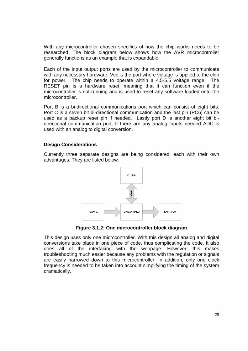
Currently three separate designs are being considered, each with their own advantages. They are listed below:

Figure 3.1.2: One microcontroller block diagram

This design uses only one microcontroller. With this design all analog and digital conversions take place in one piece of code, thus complicating the code. It also does all of the interfacing with the webpage. However, this makes troubleshooting much easier because any problems with the regulation or signals are easily narrowed down to this microcontroller. In addition, only one clock frequency is needed to be taken into account simplifying the timing of the system dramatically.

30

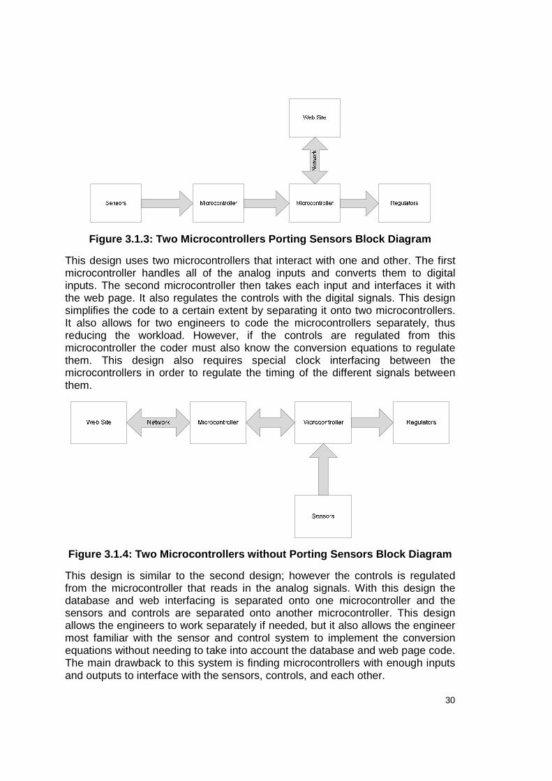
Figure 3.1.3: Two Microcontrollers Porting Sensors Block Diagram

This design uses two microcontrollers that interact with one and other. The first microcontroller handles all of the analog inputs and converts them to digital inputs. The second microcontroller then takes each input and interfaces it with the web page. It also regulates the controls with the digital signals. This design simplifies the code to a certain extent by separating it onto two microcontrollers. It also allows for two engineers to code the microcontrollers separately, thus reducing the workload. However, if the controls are regulated from this microcontroller the coder must also know the conversion equations to regulate them. This design also requires special clock interfacing between the microcontrollers in order to regulate the timing of the different signals between them.

Figure 3.1.4: Two Microcontrollers without Porting Sensors Block Diagram

This design is similar to the second design; however the controls is regulated from the microcontroller that reads in the analog signals. With this design the database and web interfacing is separated onto one microcontroller and the sensors and controls are separated onto another microcontroller. This design allows the engineers to work separately if needed, but it also allows the engineer most familiar with the sensor and control system to implement the conversion equations without needing to take into account the database and web page code. The main drawback to this system is finding microcontrollers with enough inputs and outputs to interface with the sensors, controls, and each other.

31

After considering each of the three above designs, the first design was the one implemented in the system. It was chosen because although it uses more complicated code it only requires the engineers to learn coding for one microcontroller. In addition, if only one microcontroller is used it reduces delay times between the boards connecting to each other and passing data. It also allows for a simpler hardware design and eliminates the need for clocked data to be passed precisely making it easier for the sensors and regulators to interact.

Component Selection

ATmega168

The ATmega168 is a high performance low power 8-bit microcontroller from Atmel. This chip is used to take in inputs from the sensors and send outputs to the regulating devices. It uses advanced RISC architecture and offers up to 20 MIPS throughput at 20MHz. It also offers 16 kilobytes of in-system programmable flash memory for storage of code and other uses. It also contains an on-chip analog comparator, which is useful for the sensor input comparisons. The chip has 6 analog inputs that interact with the sensors from the system. The system utilizes the analog to digital conversion and the multiple programmable I/O lines on the ATmega168. The system may also utilize the six pulse width modulation channels to read outputs from any digital sensors. Since it is low power (1.8-5.5V) consumption it is easy to create a power supply for the chip. 13

Figure 3.1.5: Arduino Diecimila development board Permission pending from Arduino

The chip can be programmed using the Arduino Diecimilia development board. This development board provides LEDs, buttons and already wired ports to help program the microcontroller initially. The USB protocol on the board allows it to be easily programmed from most modern computers so that it may be worked on efficiently. This board also gives the option to use RS-232 through an ISCP interface to program the ATmega chip in system. Arduino provides free software specifically used to for their boards. It is a cross-platform Java program that allows users to edit the code, compile it, and transfer firmware to the board. The language used by the Arduino development board is a C-like language based on the Processing language. The Processing language is used to introduce programming to coders that are not familiar with software development. It also

13

Used with permission pending from Atmel see Appendix A

32

enables the engineers to avoid using assembly code as it is not a common skill and can be tedious to program. This is ideal for creating the system so that all engineers is able to easily learn how to program and use the board.14

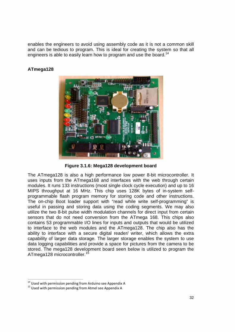
ATmega128

Figure 3.1.6: Mega128 development board

The ATmega128 is also a high performance low power 8-bit microcontroller. It uses inputs from the ATmega168 and interfaces with the web through certain modules. It runs 133 instructions (most single clock cycle execution) and up to 16 MIPS throughput at 16 MHz. This chip uses 128K bytes of in-system self-programmable flash program memory for storing code and other instructions. The on-chip Boot loader support with “read while write self-programming” is useful in passing and storing data using the coding segments. We may also utilize the two 8-bit pulse width modulation channels for direct input from certain sensors that do not need conversion from the ATmega 168. This chips also contains 53 programmable I/O lines for inputs and outputs that would be utilized to interface to the web modules and the ATmega128. The chip also has the ability to interface with a secure digital reader/ writer, which allows the extra capability of larger data storage. The larger storage enables the system to use data logging capabilities and provide a space for pictures from the camera to be stored. The mega128 development board seen below is utilized to program the ATmega128 microcontroller.15

14

Used with permission pending from Arduino see Appendix A 15

Used with permission pending from Atmel see Appendix A

33

System Integration

The ATmega168 is used in the system because of the simplicity of the programming language for the Arduino board and the availability of prewritten code for interfacing. Using the board also reduces cost in the system because the board was donated and the chip is a DIP package which allows the engineers to use one development board to program multiple microcontrollers. The connection to the Arduino board is USB which allows easier access to program the board if needed because serial ports are seldom found on new computers anymore. The ATmega168 is implemented in the system because it bests meets the requirements of the system and keeps the cost of the overall unit to a minimum.

3.2 Networking Introduction

Interfacing the system with a web-based interface can take on many different forms. The user uses the internet to connect to the system and change the various parameters, as well as view current parameters and current conditions of the growth environment. The system also has some sort of server interface where the user can view a log of the past conditions of the growth environment and keep a database of preset growth characteristics for different plant types. With such a large variety of uses, different network layouts for connectivity and data storage should be looked into.

Design Considerations

Network Layouts

Figure 3.2.1: Network Layout without wireless adapt er

This method allows for a connection to a web page that is hosted on a server that is external to a plant feeder network. This server can be hosted on the senior design web site or an external data server that would require a monthly fee. All data logging capabilities would be stored on the feeder locally and then uploaded nightly to the host server, so that the user would be able to view the data from past events. The user would also be able to check the current growth conditions from the web site, however since the host server is separate from the actual system it requires a transfer delay for the data. Another drawback to this method would be that any changes made would take some time to update because of the multiple connections being formed.

34

Figure 3.2.2: Network Layout with wireless adapter

This method is similar to the one above except it also contains the possibility of using Ethernet or an RF connection to the router. By using an Ethernet protocol to connect to the router, the system has an increased transfer rate and a more stable connection. Even though the number of components added to this method seems like a lot, it would actually decrease the overall cost of the system because finding an Ethernet controller to interface with microcontroller is significantly cheaper than actually finding a 802.11 module to interface with the microcontroller.

Local RouterHost

ServerWeb Page Local Server

Feeder

Logical Internet Wifi/RJ45

Figure 3.2.3: Network Layout with local server

This method provides a local server for the feeder, such as a computer. The computer would then do all of the interfacing with the system. Although a computer may cost more than the first two methods, this method allows the user the option to go directly to the local computer and make any changes they may require. Giving the user the option to locally use the system could allow for better troubleshooting options and decrease delay time if immediate changes need to be made to the system.

PC FeederRF/Serial/USB

Figure 3.2.4: Network Layout with direct connection

35

This method is the same as above, however eliminates the use of the web page. This is the most simplified version of for the system and is useful if the user does not need remote access.

Figure 3.2.5: Network Layout with server on plant f eeder

This method integrates the server into the plant feeder itself. Therefore whenever a connection is made to the webpage, the user is actually connecting directly to the system. With this system in place only one connection is made and it simplifies the system while still allowing for wireless web access. It also allows for faster access to the data because only one connection is being created. This method eliminates the external host, thus doing away with reliability on external services for the system. The system would be integrated into one unit allowing portability and reliability.

Component Selection

Figure 3.2.6: Lantronix MatchPort b/g Pro (Reproduced with permission from Lantronix)

To reduce cost of the overall project the MatchPort b/g Pro was donated by Lantronix and is used in the system. The MatchPort b/g Pro is the gateway to the internet for our microcontroller and also hosts the web page. This solution to networking provides an on-chip data server with 802.11 b/g capabilities. It also contains a dedicated co—processor module that manages wireless connectivity and web services, which lets the on-board microcontroller to function as its highest capacity. As long as the microcontroller selected contains a serial interface, which most do, Lantronix boasts its module is able to interact with it. The MatchPort b/g Pro contains exclusive SmartRoam technology which continuously tracks signal strength within range and automatically connects to the access point with the strongest signal. This is beneficial in always making sure the system has the strongest connection possible.

Since the MatchPort b/g Pro is hosting the systems web page it is necessary to use the modules web server for hosting capabilities. The module uses Lantronix trademarked Evolution OS operating system, which has integrated CGI-capable

36

web server that allows the user to remotely monitor the data through the web browser. There is a web page overlay on this system for user friendly access. The module also supports open management standards for the web page such as “Cisco-like” CLI, XML, and serial and Telnet options.16

3.3 Software User Interface Introduction The software user interface allows the user to select from a database or input user defined values for the plant(s) that they would like to grow. The system uses a web browser to allow the user to interact. The database is comprised of different general plants that are grown in this size of container such as, sunflowers, tomatoes, lettuce and assorted herbs. Device Selection The system is using the Lantronix MatchPort b/g Pro for wireless interfacing which comes with an onboard data server. The system is using the data server to host its web page. The MatchPort offers a CGI-capable web server that allows the device to be controlled wirelessly using the Lantronix Evolution OS. There is a web page overlay on the data server to make it more user friendly. The Evolution OS uses AJAX technology to give the user smooth browsing of active content. The MatchPort also allows administrators to manage the device and web page through open standards such as CLI, XML, and serial and Telnet options. Since the system does not want all users to be able to access the web page and change growing parameters the system implements a security system. The Lantronix also incorporates data protection using the IEEE 802.11i with AES-CCMP and TKIP encryption. It contains all of the 802.1x Enterprise Authentication Protocols (EAP) and end-to-end AES 128-bit encrypted tunneling.17 The system itself provides features such as real time display of all measurements. Since the data needs to be taken from the sensors and the microcontroller the real time data is delayed by transfer times and general internet connection delays. Along with the real time display there is a data log of all plant growth history for a defined amount of time depending on the data storage capabilities. The data log displays time stamps, date, CO2 levels, level of solution in the system, feeding method being used, humidity in the air, temperature, the amount of nutrients in the system and the pH of the solution. The user is able to define certain environment specifications for the system. They is able to fill or drain the feeding solution, select different feeding methods for the

16

This information has been used with permission from Lantronix see Appendix A. 17

Used with permission from Lantronix see appendix A.

37

plant. The user can also define day and night cycles for the lighting to optimize light absorption by the plant. The user is also able to regulate the pH of the feeding solution and the nutrient level of the feeding solution.

Chapter 4: Regulation

4.1 Lighting System 4.1.1 Light Source Introduction

Because choosing a light source is one of the more critical parts of this project, it was necessary to first consider what makes light so important in order to determine the best type of light source that could be used to optimize growth. The main properties of light that affect the plant growth are intensity, duration and quality. Knowing the intensity of the light helps to determine how far or close the light source should be from the plant based on the type of plant that is used in the project. This intensity is both proportional to the power of the light source and inversely proportional to the distance of the plant from the source. The desired power which provides this intensity should be between 20 and 50 W where lower wattage would be used for low light plants and the higher for high light plants. Because the system should be used in areas where indirect sunlight is available, the light source merely acts as supplementary lighting which does not require the light source to provide maximum wattage. In addition to the necessary 16 to 18 hours of light a plant needs a day, it also important to provide a period of darkness. With this in mind, a timer circuit should be provided so as to allow for these durations to take place. The ideal cycle would consist of being on during the day so as to allow supplementary lighting in the house and to turn off at night. Of the three properties of light, the quality of the light seemed to have the largest impact on a plants growth. Even though sunlight provides the entire spectrum of visible light to the plant, only certain parts of this spectrum are utilized by the plant in the photosynthesis process. The main ranges of wavelengths that are absorbed by the plant primarily consist of the blue and red spectrums as seen in the figure 4.1.1.1 below.

Figure 4.1.1.1: Useful Spectrum for Photosynthesis Used with permission from Ars-Informatica

38

Design Considerations

In choosing a light source for this project, the main factors being considered are those described in the introduction, as well as heat emission, power consumption, cost and longevity of life. The main types of light sources available that have been considered in this project are incandescent, cool-white, HID and LED. Incandescent and cool-white were quickly dismissed as possible lighting sources as the incandescent only provides mainly red spectrum of light while the cool-white is barely into the blue portion of the spectrum. Both are good for supplementary lighting and are typically only used during specific stages of growth. The HID lights, which can be found in most professional greenhouses, offer a decent spread of the spectrum needed by plants as well as intensity. Based on many of the products that were available however, this solution can quickly become expensive in addition to the large amounts of power needed. After some consideration, LED’s seemed to be the best choice for the job as they have the ability to offer a dynamic range of spectrum with color mixing, have low heat dissipation, low power consumption and a lower cost. The only down fall seemed to be the intensity. As the available intensity of the LED grow light increased so did the price. However, as previously discussed intensity can also be increased and decreased relative to the distance from the plant.

Component Selection

Figure 4.1.1.2: LED LIght

The light source chosen for this project is an LED grow panel which contains more than 225 red and blue led’s combined, has the following specifications:

Description Specification Operating Voltage 110/120 VACrms

Operating Current 115 mArms

Operating Power 13.8 W Dimensions 12.25 x 12.25 x 1.25 in Cord length 48 in Min. Placement above Plant 3 in Max Placement above Plant 24 in Cost $43.00

Table 4.1.1.1: Light Source Specifications

39

The component was selected for a number of reasons which include providing the necessary wavelengths of light, low cost, light weight, low power consumption and low heat dissipation. The wavelengths of the LED’s are rated at 465 nm for the Red and 650 nm for the blue. Given these values one can see from table 4.1.1.1 that they meet the criteria for useful lighting. Compared to other LED sources found, this particular source is about half the cost. Though it loses some quality compared to their higher costing counterparts, it serves its purpose as far as showing how the light would operate in a marketable unit. The weight is essential as a heavier unit would require a larger motor for automated adjustment purposes which is discussed in the sections to follow. As stated before the power consumption is just another factor that comes into play in any electrical design where operating costs are a concern. The heat dissipation of this unit allows it to be placed closely to the plants and without the concern of causing any damage to the plants.

System Integration

Figure 4.1.1.3: Light Source Connection Diagram

The light source is controlled through the use of a relay and microcontroller as shown in figure 4.1.1.3. The type of relay used in this situation should be “Normally Closed” due to energy efficiency. Because the relay is passing power to the light source for a longer period during the day than at night, it would make more sense to have a Normally Closed condition. Therefore the microcontroller would be using less energy to keep the relay open. The type of relay used in this situation does not matter as long as it is meets the necessary rating to provide power to the light source.

4.1.2 Adjustment Introduction

An important decision to make with the setup of the light system was how to compensate for the distance from the light to the plant as the plant grows. For the

40

simplest setup, the light source could be made to manually increase or decrease in distance from the plant which would be a task required by the user of the system. The second method was to incorporate an automated system that would go with the scheme of the project allowing for adjustment without the help of the system user. Both methods have been considered for this project; however the first of the two would simply be a backup in the event that the second cannot be accomplished by the deadline.

Design Considerations.

For both methods discussed below, the main concerns were how to devise a support system that would accommodate each method for both ease of implementation and proper support of the light source.

Manual Adjustment

For this method there were two different kinds of setups that were considered. The first is a fixed support structure where the supports themselves are raised and lowered in accordance with the desired height as seen in the figure below.

Figure 4.1.2.1: Manual Adjustment using a combinati on of Fixed and Adjustable Supports

The figure 4.1.2.1 shows two types of supports. The bottom support would be fixed to the feeder structure while the upper support would be adjustable and fixed to the light source. In between the two supports would be a locking mechanism that tightens and loosens, allowing for the adjustable support to become fixed according to the desired height.

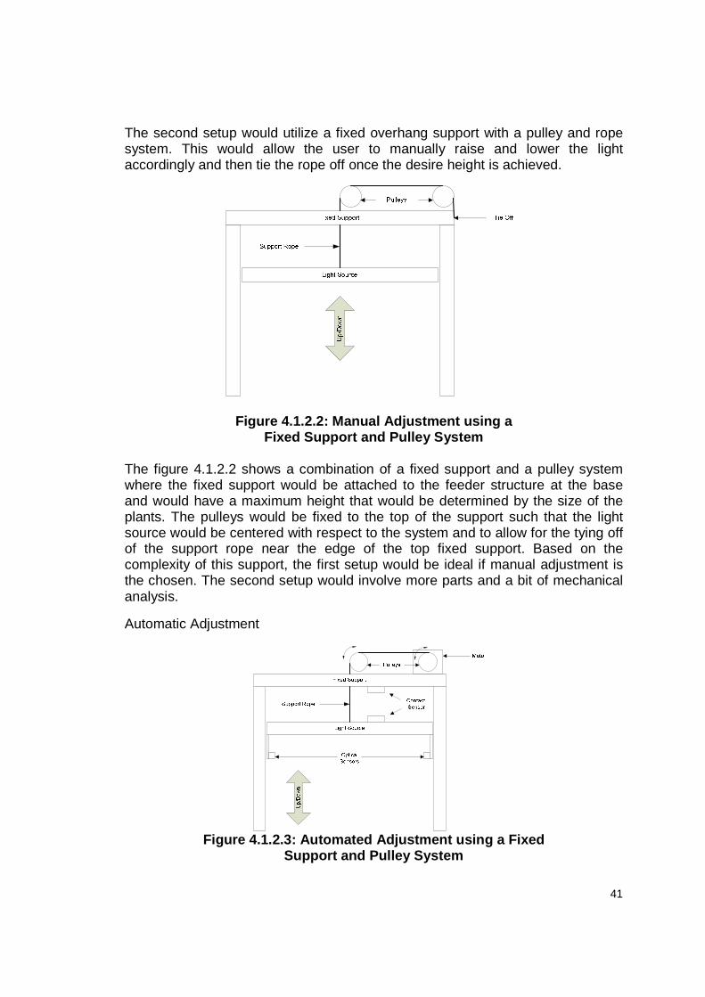
41

The second setup would utilize a fixed overhang support with a pulley and rope system. This would allow the user to manually raise and lower the light accordingly and then tie the rope off once the desire height is achieved.

Figure 4.1.2.2: Manual Adjustment using a Fixed Support and Pulley System

The figure 4.1.2.2 shows a combination of a fixed support and a pulley system where the fixed support would be attached to the feeder structure at the base and would have a maximum height that would be determined by the size of the plants. The pulleys would be fixed to the top of the support such that the light source would be centered with respect to the system and to allow for the tying off of the support rope near the edge of the top fixed support. Based on the complexity of this support, the first setup would be ideal if manual adjustment is the chosen. The second setup would involve more parts and a bit of mechanical analysis.

Automatic Adjustment

Figure 4.1.2.3: Automated Adjustment using a Fixed

Support and Pulley System

42

For this method, only one setup was considered which is very similar to the second manual adjustment setup. In this case, the tie off location would be eliminated and the pulley near the edge of the support would be controlled by a motor as seen in the figure 4.1.2.3 above. In addition to the motor, it was decided that a contact sensor and optical sensor would be necessary to carry out the full functionality of the design. The contact sensor would be implemented to provide a reference point for the position of the light source. When the lighting system is first initiated, the light source would be “zeroed” at the maximum height of the support where the contact sensors meet and would then be slowly lowered by the motor until the height of the plant is reached. When the optical sensor is breached by the presence of the plant, it triggers the stopping of the motor. The motor is then reversed so as to move the light source up by a small distance. As the plant continues to grow, the process seen in the figure below is repeated. Once the maximum height of the system has been reached, automation discontinues and a message to the user is provided at login as shown in the flowchart below listed as figure 4.1.2.4.

Figure 4.1.2.4: Block Diagram of in-use Automated L ighting System The below flowchart listed as figure 4.1.2.5 assumes that the rope is first connected to the motor and light source and that there is in fact a plant present in the system. Additionally, the “Initiate Zero Sequence” would constitute a coded control within the software that would initiate the process. The distance of the optical sensors from the light source is determined based on the intensity of the light source and the required distance of the plant from the light source. For the use of LED’s, this should be fairly close to the plant since they would provide a lower intensity of light. Because the LED’s do not emit much heat, there is no worry of the plants being affected by the proximity of the source. The type of motor, optical sensor and contact sensor used are discussed in the following subsections sections.

43

Initiate

Zero

Sequence

Contact

Sensor

Reached

Yes

No

Stop Motor

Do Nothing

Turn on Motor

(up direction)

Turn on Motor

(Down direction)

Optical Sensor

BreachedDo NothingNo

Stop Motor

Yes

Turn on Motor for

specified time

(up direction)

Figure 4.1.2.5: Initial Setup of Automated Lighting System

4.1.3 Motor For the purpose of raising and lowering the light, three types of motors were considered: servo, stepper and continuous motors. Servo motors can offer the torque needed to lift the light source as well as precision over the change in distance but can quickly become expensive and require maintenance. Through

44

the use of a stepper motor, precise control over the height of the light source could be achieved by knowing the angular step of the motor, provide good torque at low speeds and are somewhat low cost. With a continuous motor, the precision of the previous two is not quite as good; however at low speeds the motor could be precisely stopped when needed. In all cases, since the speed would vary with respect to the voltage applied, a lower applied voltage would be necessary so that a slow transition takes place to allow for more precise stopping and a larger applied torque. In addition, it would be necessary to have a motor that is bi-directional to allow for the up and down motion. In the consideration of each type of motor, the torque that the each supplies was a main consideration when choosing the right one. To provide enough leeway for the motor to operate efficiently, a weight of 10 lbs/4.5 kg was assumed to be the necessary lifting capacity of the motor given that the weight of the light source is around 3 lbs plus a small amount of weight of additional hardware and sensors. Knowing the weight capacity, the torque required by the motor for proper use could be determined. For convenience of units and specs on many of the motors, SI units were used as the base of measurement. Given that the average size of the rotor which extends from the motor for the size needed in this project is around 1 cm, a torque of approximately 4.5 kg*cm was established as the requirement. For the light to be held stationary it is necessary to figure out a means of supporting the lighting while not putting any strain on the motor. To optimize the life of the motor it would not be beneficial to employ a solution such that a voltage would be applied to allow for no rotation and a constant holding torque. A few of the methods considered were through the use of a winch-type system that is seen on the front of off-road vehicles which are used for pulling heavy objects. The problem with this type of setup is that these motors are typically only operated at one speed and one direction. Thus this would not meet the requirements of this system. Another approach is using a hoisting system like those used in lifting engines out of vehicles. This method provides bi-directional motion as required, but the overall assemblies found on the market are quite bulky and costly. There were some units that were found costing between $60 and $100 which could be used in the event other methods failed. The final method that has been considered is through the use of “special” gears known as worm gears. These gears were discovered when analyzing the system that makes a car window move up and down. They are designed such that force a linear force is applied to the motor and not a rotational force. As seen in the Figure 4.1.3.1, the worm is on top while the gear is on the bottom. The worm can easily turn the gear while the opposite is not true. As long as the motor is secured tightly to the structure, the gear stays in place causing the light source and all attached components to remain stationary.

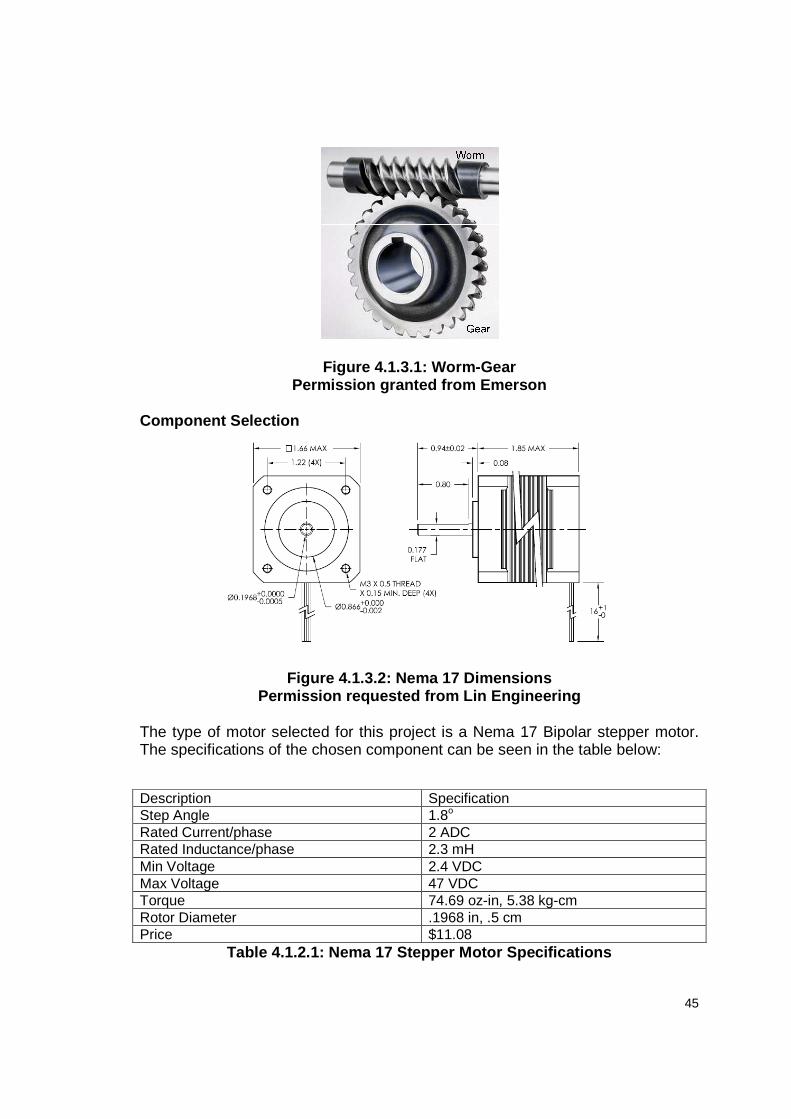
45

Figure 4.1.3.1: Worm-Gear Permission granted from Emerson

Component Selection

Figure 4.1.3.2: Nema 17 Dimensions Permission requested from Lin Engineering

The type of motor selected for this project is a Nema 17 Bipolar stepper motor. The specifications of the chosen component can be seen in the table below:

Description Specification Step Angle 1.8o Rated Current/phase 2 ADC Rated Inductance/phase 2.3 mH Min Voltage 2.4 VDC Max Voltage 47 VDC Torque 74.69 oz-in, 5.38 kg-cm Rotor Diameter .1968 in, .5 cm Price $11.08

Table 4.1.2.1: Nema 17 Stepper Motor Specifications

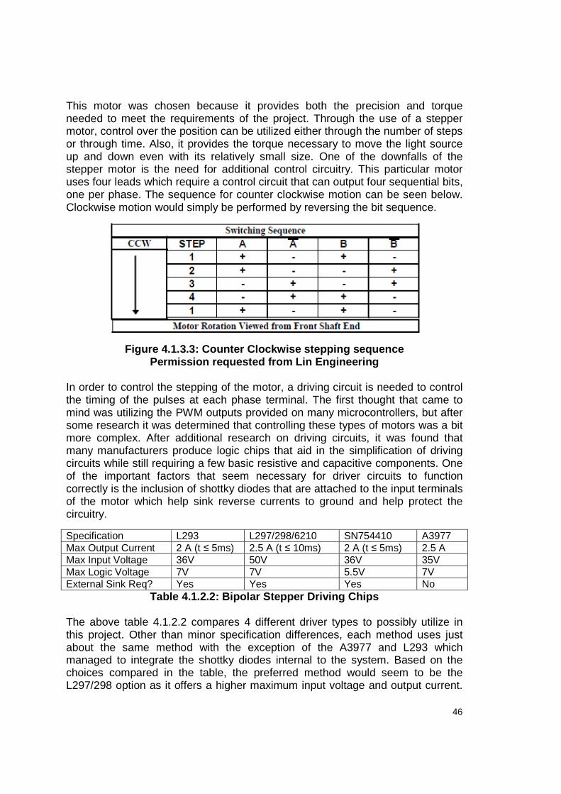
46

This motor was chosen because it provides both the precision and torque needed to meet the requirements of the project. Through the use of a stepper motor, control over the position can be utilized either through the number of steps or through time. Also, it provides the torque necessary to move the light source up and down even with its relatively small size. One of the downfalls of the stepper motor is the need for additional control circuitry. This particular motor uses four leads which require a control circuit that can output four sequential bits, one per phase. The sequence for counter clockwise motion can be seen below. Clockwise motion would simply be performed by reversing the bit sequence.

Figure 4.1.3.3: Counter Clockwise stepping sequence Permission requested from Lin Engineering

In order to control the stepping of the motor, a driving circuit is needed to control the timing of the pulses at each phase terminal. The first thought that came to mind was utilizing the PWM outputs provided on many microcontrollers, but after some research it was determined that controlling these types of motors was a bit more complex. After additional research on driving circuits, it was found that many manufacturers produce logic chips that aid in the simplification of driving circuits while still requiring a few basic resistive and capacitive components. One of the important factors that seem necessary for driver circuits to function correctly is the inclusion of shottky diodes that are attached to the input terminals of the motor which help sink reverse currents to ground and help protect the circuitry.

Specification L293 L297/298/6210 SN754410 A3977 Max Output Current 2 A (t ≤ 5ms) 2.5 A (t ≤ 10ms) 2 A (t ≤ 5ms) 2.5 A Max Input Voltage 36V 50V 36V 35V Max Logic Voltage 7V 7V 5.5V 7V External Sink Req? Yes Yes Yes No

Table 4.1.2.2: Bipolar Stepper Driving Chips

The above table 4.1.2.2 compares 4 different driver types to possibly utilize in this project. Other than minor specification differences, each method uses just about the same method with the exception of the A3977 and L293 which managed to integrate the shottky diodes internal to the system. Based on the choices compared in the table, the preferred method would seem to be the L297/298 option as it offers a higher maximum input voltage and output current.

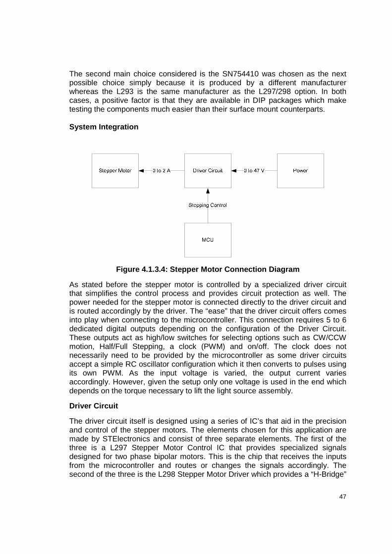
47

The second main choice considered is the SN754410 was chosen as the next possible choice simply because it is produced by a different manufacturer whereas the L293 is the same manufacturer as the L297/298 option. In both cases, a positive factor is that they are available in DIP packages which make testing the components much easier than their surface mount counterparts. System Integration

Figure 4.1.3.4: Stepper Motor Connection Diagram

As stated before the stepper motor is controlled by a specialized driver circuit that simplifies the control process and provides circuit protection as well. The power needed for the stepper motor is connected directly to the driver circuit and is routed accordingly by the driver. The “ease” that the driver circuit offers comes into play when connecting to the microcontroller. This connection requires 5 to 6 dedicated digital outputs depending on the configuration of the Driver Circuit. These outputs act as high/low switches for selecting options such as CW/CCW motion, Half/Full Stepping, a clock (PWM) and on/off. The clock does not necessarily need to be provided by the microcontroller as some driver circuits accept a simple RC oscillator configuration which it then converts to pulses using its own PWM. As the input voltage is varied, the output current varies accordingly. However, given the setup only one voltage is used in the end which depends on the torque necessary to lift the light source assembly.

Driver Circuit

The driver circuit itself is designed using a series of IC’s that aid in the precision and control of the stepper motors. The elements chosen for this application are made by STElectronics and consist of three separate elements. The first of the three is a L297 Stepper Motor Control IC that provides specialized signals designed for two phase bipolar motors. This is the chip that receives the inputs from the microcontroller and routes or changes the signals accordingly. The second of the three is the L298 Stepper Motor Driver which provides a “H-Bridge”

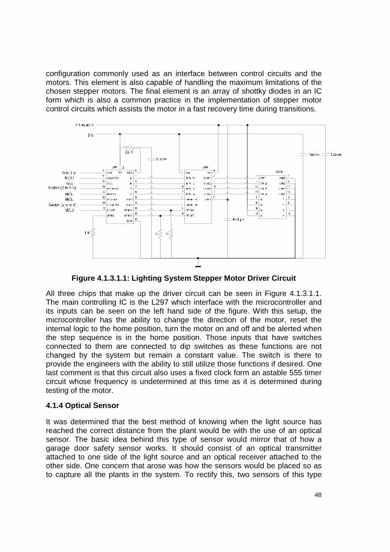
48

configuration commonly used as an interface between control circuits and the motors. This element is also capable of handling the maximum limitations of the chosen stepper motors. The final element is an array of shottky diodes in an IC form which is also a common practice in the implementation of stepper motor control circuits which assists the motor in a fast recovery time during transitions.

Figure 4.1.3.1.1: Lighting System Stepper Motor Dri ver Circuit

All three chips that make up the driver circuit can be seen in Figure 4.1.3.1.1. The main controlling IC is the L297 which interface with the microcontroller and its inputs can be seen on the left hand side of the figure. With this setup, the microcontroller has the ability to change the direction of the motor, reset the internal logic to the home position, turn the motor on and off and be alerted when the step sequence is in the home position. Those inputs that have switches connected to them are connected to dip switches as these functions are not changed by the system but remain a constant value. The switch is there to provide the engineers with the ability to still utilize those functions if desired. One last comment is that this circuit also uses a fixed clock form an astable 555 timer circuit whose frequency is undetermined at this time as it is determined during testing of the motor.

4.1.4 Optical Sensor It was determined that the best method of knowing when the light source has reached the correct distance from the plant would be with the use of an optical sensor. The basic idea behind this type of sensor would mirror that of how a garage door safety sensor works. It should consist of an optical transmitter attached to one side of the light source and an optical receiver attached to the other side. One concern that arose was how the sensors would be placed so as to capture all the plants in the system. To rectify this, two sensors of this type

49

would be incorporated such that each would line up with an array of plants as seen in the figure below.

Figure 4.1.4.1: Top View of Optical Sensor Field

As one can see, this setup can allow for one sensor and transmitter per array of plants which would capture the tallest plant in each array. Since all plants use the same available light source, the result would be that if either sensor is breached the light would be adjusted to compensate for the fastest growing plant in both arrays.

Based on the type of sensors used in this setting, infrared wavelengths would be the most likely used source and could be implemented in a form where the sensors themselves are already encased, as in the garage door example, or in a form where they need to be soldered and encased. Being that the two sensors would be separate from one another and must be encased for protection as well as mounting purposes, finding them already encased would be more beneficial and save time in the implementation of the devices.

One thing that must be kept in mind during setup is to assure that these sensors are accurately aligned when attaching them and that support is provided so that when the light is in motion, these sensors do not come loose from their positions and lose sight from one another. In such a case, the prolonged period in which the sensors did loose contact would be monitored by the system and would promptly notify the user. During normal operation, the amount of time taken for the plant to breach the field and for the lighting system to respond should not be more than a few seconds, therefore anything longer than this would indicate a misplacement of the optical field(s).

Component Selection

The component that was chosen for this part of the lighting system is a Short Range proximity sensor made by Sharp with the specifications listed below:

50

Description Specification Maximum Supply Voltage (VCC) 7 VDC Recommended Supply Voltage 4.5 to 5.5 VDC Maximum Output Voltage VCC + .3 Minimum Distance 3 cm Maximum Distance 40 cm Cost $13.95

Table 4.1.2.3: Optical Sensor Specifications

Typically, this sensor is used to determine the distance of an object from the sensor; however its use is only for the presence or absence of an object within its line of sight, particularly a plant. The only advantage to choosing this sensor was its low cost compared to other sensors that offer the same function.

System Integration

The main idea behind this sensor is provide a signal when an object breaches its path. Because the transmitter and sensor are both in the same circuit, a reflector is required to maintain a reference distance in the system. When the distance measured is less than the reference, this is an indicator that the path has in fact been breached. A diagram of the setup can be seen below.

Figure 4.1.4.2: Optical Sensor Setup

As seen in the figure above, the sensor is attached to a bracket which has been displaced by a distance of 3 cm. The purpose of this distance is to allow for the minimum detection distance to be within the area of the light source. On the opposite side of the light source is the location of the reflector which sets the reference point. This distance provides a constant voltage which can be used as a measure against a change in voltage due to the presence of an object. When an object is present the voltage increases and therefore alerts to the presence of an object. Because the purpose of the sensor is merely to detect the presence/absence of an object, the analog output of the sensor can be made digital through the use of a comparator. The positive terminal of the comparator is connected to the output voltage of the sensor while the negative terminal is connected to a reference voltage (Vref) which is 1.1 times the voltage measured

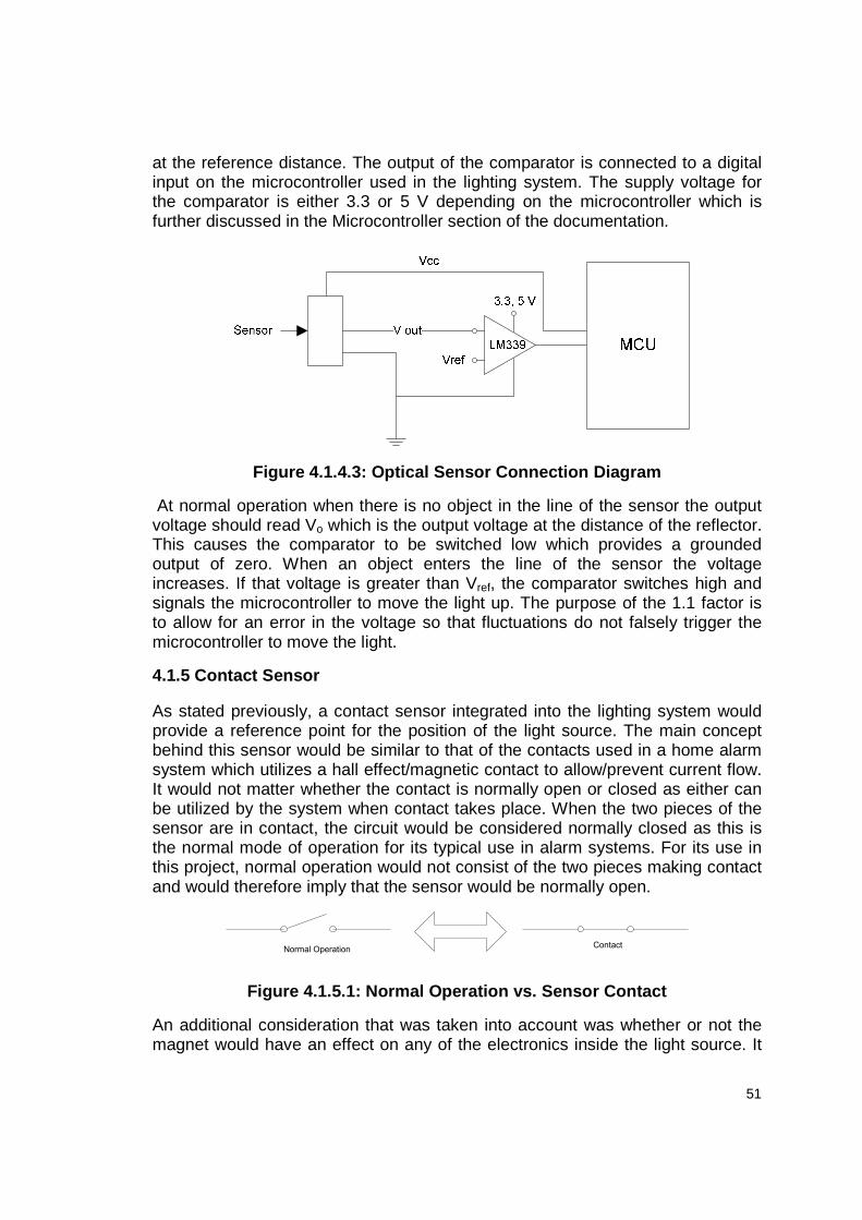
51

at the reference distance. The output of the comparator is connected to a digital input on the microcontroller used in the lighting system. The supply voltage for the comparator is either 3.3 or 5 V depending on the microcontroller which is further discussed in the Microcontroller section of the documentation.

Figure 4.1.4.3: Optical Sensor Connection Diagram

At normal operation when there is no object in the line of the sensor the output voltage should read Vo which is the output voltage at the distance of the reflector. This causes the comparator to be switched low which provides a grounded output of zero. When an object enters the line of the sensor the voltage increases. If that voltage is greater than Vref, the comparator switches high and signals the microcontroller to move the light up. The purpose of the 1.1 factor is to allow for an error in the voltage so that fluctuations do not falsely trigger the microcontroller to move the light.

4.1.5 Contact Sensor As stated previously, a contact sensor integrated into the lighting system would provide a reference point for the position of the light source. The main concept behind this sensor would be similar to that of the contacts used in a home alarm system which utilizes a hall effect/magnetic contact to allow/prevent current flow. It would not matter whether the contact is normally open or closed as either can be utilized by the system when contact takes place. When the two pieces of the sensor are in contact, the circuit would be considered normally closed as this is the normal mode of operation for its typical use in alarm systems. For its use in this project, normal operation would not consist of the two pieces making contact and would therefore imply that the sensor would be normally open.

Normal OperationContact

Figure 4.1.5.1: Normal Operation vs. Sensor Contact

An additional consideration that was taken into account was whether or not the magnet would have an effect on any of the electronics inside the light source. It

52

was determined that these types of sensors are actually designed in such a way as to reduce the amount of flux on one side of the sensor and increase it on the contact side. However, as a precautionary measure it was decided that the sensor be placed on the light source at some position around its perimeter, preferably in a location where the source power is not.

Component Selection

There are two components which have been chosen to be tested for implementation in this project. The first is a basic magnetic hall-effect sensor from General Electric which is used as contacts in security systems. The second is a digital effect sensor which can be configured in either pull-up or pull down mode. The specifications for each are provided below.

Description Specification Switch Configuration N.O. Maximum Supply Voltage 100 V(AC/DC) Maximum Supply Current .5 A(AC/DC) Resistance .2 Ω Response Time 1 ms

Table 4.1.5.1: GE Hall-Effect Sensor Specifications

Description Specification Switch Configuration N.O. Operating Supply Voltage 4.5 – 24 VDC Maximum Output Voltage 500 mV Maximum Output Current 12 mADC

Table 4.1.5.2: Digital Hall-Effect Sensor Specifica tions

Both sensors provide a normally open configuration meaning that when the contact magnet is in range, the device does not allow current to pass. Because this device serves such a simple purpose, there was really no way to distinguish which one would better serve its purpose in this project. The GE sensor is considered an analog device however it can be operated within the range of the microcontroller voltage and act as a digital input using DC sourcing. The disadvantage to this device is that it can only provide a high-to-low input, whereas the digital sensor can be configured to provide high-to-low or low-to-high. On the other hand, the digital sensor only outputs a maximum voltage of .5 which would require amplification.

System Integration

For the implementation in the project it would be preferred to have an input signal to the microcontroller that goes from low-to-high. Thus, the GE sensor would need an additional element to switch its operation. Below are the configuration diagrams for both sensors.

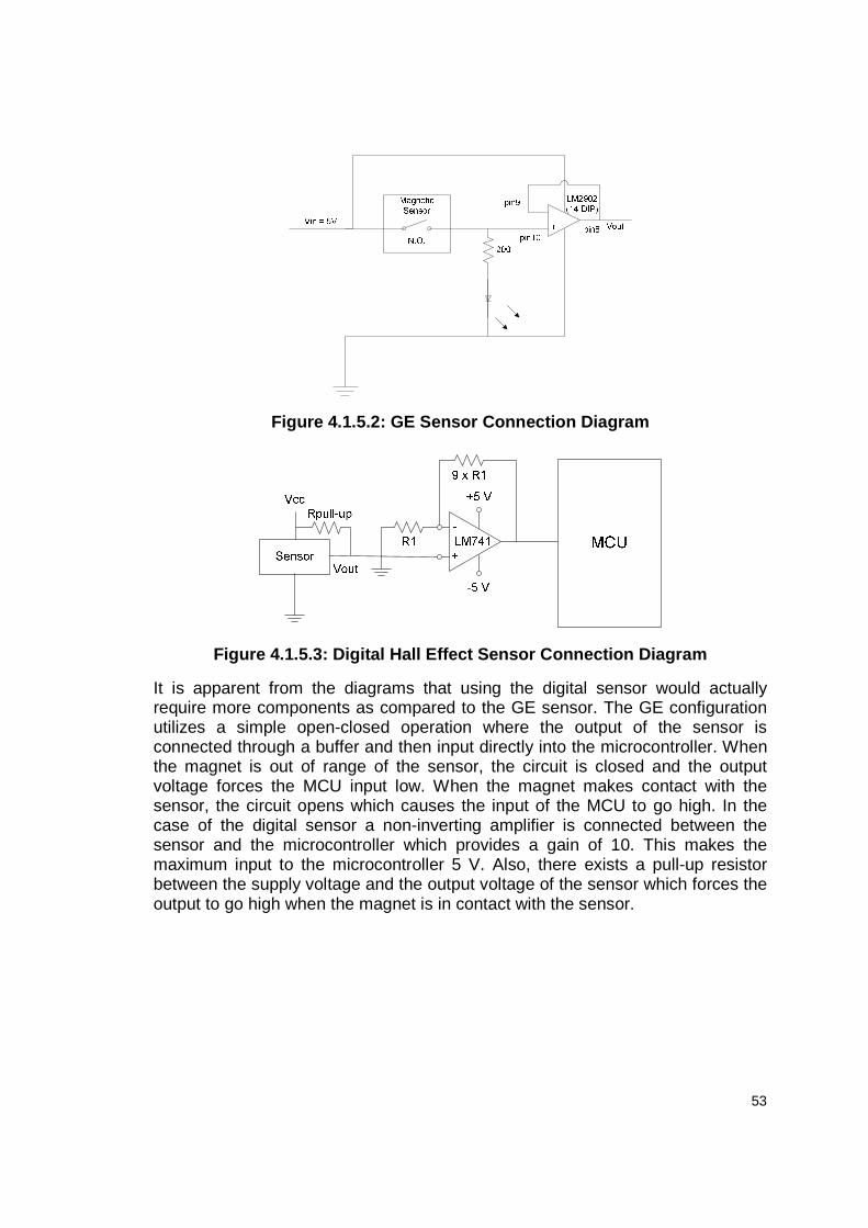
53

Figure 4.1.5.2: GE Sensor Connection Diagram

Figure 4.1.5.3: Digital Hall Effect Sensor Connecti on Diagram

It is apparent from the diagrams that using the digital sensor would actually require more components as compared to the GE sensor. The GE configuration utilizes a simple open-closed operation where the output of the sensor is connected through a buffer and then input directly into the microcontroller. When the magnet is out of range of the sensor, the circuit is closed and the output voltage forces the MCU input low. When the magnet makes contact with the sensor, the circuit opens which causes the input of the MCU to go high. In the case of the digital sensor a non-inverting amplifier is connected between the sensor and the microcontroller which provides a gain of 10. This makes the maximum input to the microcontroller 5 V. Also, there exists a pull-up resistor between the supply voltage and the output voltage of the sensor which forces the output to go high when the magnet is in contact with the sensor.

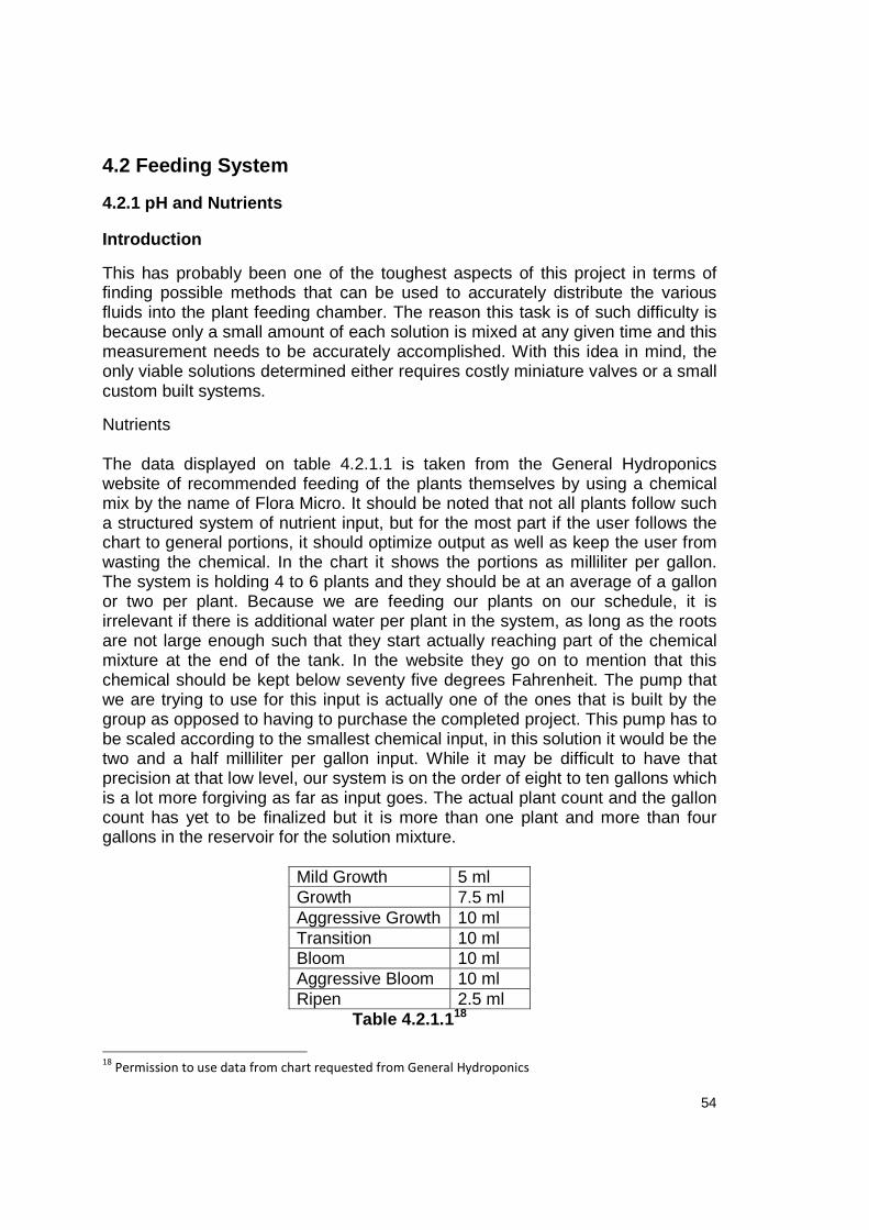
54

4.2 Feeding System 4.2.1 pH and Nutrients Introduction

This has probably been one of the toughest aspects of this project in terms of finding possible methods that can be used to accurately distribute the various fluids into the plant feeding chamber. The reason this task is of such difficulty is because only a small amount of each solution is mixed at any given time and this measurement needs to be accurately accomplished. With this idea in mind, the only viable solutions determined either requires costly miniature valves or a small custom built systems.

Nutrients The data displayed on table 4.2.1.1 is taken from the General Hydroponics website of recommended feeding of the plants themselves by using a chemical mix by the name of Flora Micro. It should be noted that not all plants follow such a structured system of nutrient input, but for the most part if the user follows the chart to general portions, it should optimize output as well as keep the user from wasting the chemical. In the chart it shows the portions as milliliter per gallon. The system is holding 4 to 6 plants and they should be at an average of a gallon or two per plant. Because we are feeding our plants on our schedule, it is irrelevant if there is additional water per plant in the system, as long as the roots are not large enough such that they start actually reaching part of the chemical mixture at the end of the tank. In the website they go on to mention that this chemical should be kept below seventy five degrees Fahrenheit. The pump that we are trying to use for this input is actually one of the ones that is built by the group as opposed to having to purchase the completed project. This pump has to be scaled according to the smallest chemical input, in this solution it would be the two and a half milliliter per gallon input. While it may be difficult to have that precision at that low level, our system is on the order of eight to ten gallons which is a lot more forgiving as far as input goes. The actual plant count and the gallon count has yet to be finalized but it is more than one plant and more than four gallons in the reservoir for the solution mixture.

Mild Growth 5 ml Growth 7.5 ml Aggressive Growth 10 ml Transition 10 ml Bloom 10 ml Aggressive Bloom 10 ml Ripen 2.5 ml

Table 4.2.1.118

18

Permission to use data from chart requested from General Hydroponics

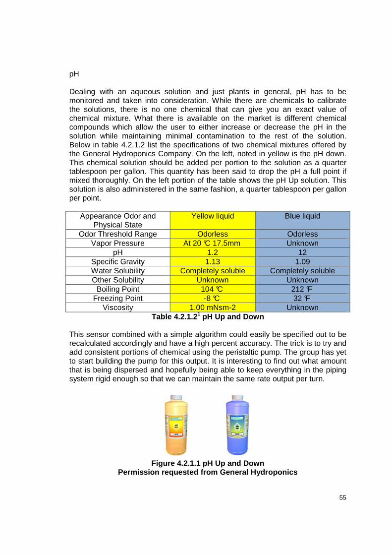
55

pH Dealing with an aqueous solution and just plants in general, pH has to be monitored and taken into consideration. While there are chemicals to calibrate the solutions, there is no one chemical that can give you an exact value of chemical mixture. What there is available on the market is different chemical compounds which allow the user to either increase or decrease the pH in the solution while maintaining minimal contamination to the rest of the solution. Below in table 4.2.1.2 list the specifications of two chemical mixtures offered by the General Hydroponics Company. On the left, noted in yellow is the pH down. This chemical solution should be added per portion to the solution as a quarter tablespoon per gallon. This quantity has been said to drop the pH a full point if mixed thoroughly. On the left portion of the table shows the pH Up solution. This solution is also administered in the same fashion, a quarter tablespoon per gallon per point.

Appearance Odor and Physical State

Yellow liquid Blue liquid

Odor Threshold Range Odorless Odorless Vapor Pressure At 20 °C 17.5mm Unknown

pH 1.2 12 Specific Gravity 1.13 1.09 Water Solubility Completely soluble Completely soluble Other Solubility Unknown Unknown

Boiling Point 104 °C 212 °F Freezing Point -8 °C 32 °F

Viscosity 1.00 mNsm-2 Unknown Table 4.2.1.21 pH Up and Down

This sensor combined with a simple algorithm could easily be specified out to be recalculated accordingly and have a high percent accuracy. The trick is to try and add consistent portions of chemical using the peristaltic pump. The group has yet to start building the pump for this output. It is interesting to find out what amount that is being dispersed and hopefully being able to keep everything in the piping system rigid enough so that we can maintain the same rate output per turn.

Figure 4.2.1.1 pH Up and Down

Permission requested from General Hydroponics

56

Design Considerations

The solution dispensing system must comprise of three separate dispensers: one for the nutrient solution, one for the pH up solution and one for the pH down solution. The idea system should have the ability to provide fluids to the feeder with zero down time. Meaning, once a solution has been exhausted into the system, the user is able to add additional fluids to the respective reservoirs without having to reset any components or the system itself. This is a desirable characteristic, but overall is not a requirement. In addition, cost and intricacy of development were taken into consideration. As a result of which ever solution is chosen, the cost of that particular method is multiplied by three which quickly increase the cost. Also, because the basis of this project is focused on electrical design, the solution must have a minimal amount of mechanical design and implementation. With this in mind, the first approach to this problem was through the use of valves that are gravity fed, followed by a few small “home-made” systems that offer the same result.

Solenoid Valves

The main idea behind the use of a solenoid valve was to provide a particular amount of solution into the feeder based on the amount of time that the solenoid was turned on for. The biggest constraint in this approach was find a valve that could allow for a small flow of liquid that could be controlled within a few milliliters. Given a valve and relay with certain response times, as well as the flow rate of the valve itself, the amount of liquid could in fact be controlled with great accuracy. With the size constraint in mind, the smaller the flow of liquid, the greater the price starts to rise. An additional constraint in the use of valves is finding the right type of valve for the right type of fluid. Because some valves a sensitive to corrosive liquids, the type of valve that could be used is also restricted. This leads to the limitation of using pinch-type valves or specialty valves which increases the cost. Of the smaller valves, also referred to as “micro” or “miniature” valves, precision could be obtained down to the micro-liter, however the price for these types of valves are high, and when multiplied by, three they are even higher but still a considerable option just in case.

The valve approach was thought of to be implemented in a few different ways. The first method consists of a single two-way valve for each reservoir where the reservoir holding the liquid is held at a higher level than the valve itself. This would provide the pressure necessary for liquid to flow through the valve and would eliminate the need for a pump. The figure below shows the reservoir at a level above the valve where the liquid is flowing down and out through the valve. This method would also allow for the solution to be refilled through the top of the reservoir for continuous operation and to allow for maximum draining of the solution into the feeder.

57

Figure 4.2.1.1: Single valve per reservoir setup (n o pump)

An alternative method using a single valve per reservoir would make use of an additional pump per valve, however would not utilize time as a form of measurement, but instead a single tube that is precut to the desired amount of fluid as seen in the figure below.

Figure 4.2.1.2: Single valve per reservoir setup (w ith pump)

As seen in the figure, a piece of pipe or tubing would stem off from the mail line that would be filled to a maximum amount allowing for the rest to run off and back into the reservoir. Once filled, the valve would be opened and the precise amount of solution would be dispensed into the feeder. The obvious problem with this approach however is its increase in intricacy as well as components. The tubing would have to be routed in such a way so that gravity would take the leftover solution back to its reservoir without the use of a second pump.

In order to minimize the number of valves used, another method to possibly be employed utilizes a four-way valve, with three inputs and one output. Obviously the cost of this type of valve is greater than that of a two-way valve, but it would cheaper than purchasing three separate valves. As in figure 4.2.1.1, this method would use gravity to provide the pressure necessary for liquid to flow through the valve and into the feeder therefore eliminating the need for pumps. Additionally, this type of valve could also be employed as in figure 4.2.1.2, which would require the use of pumps.

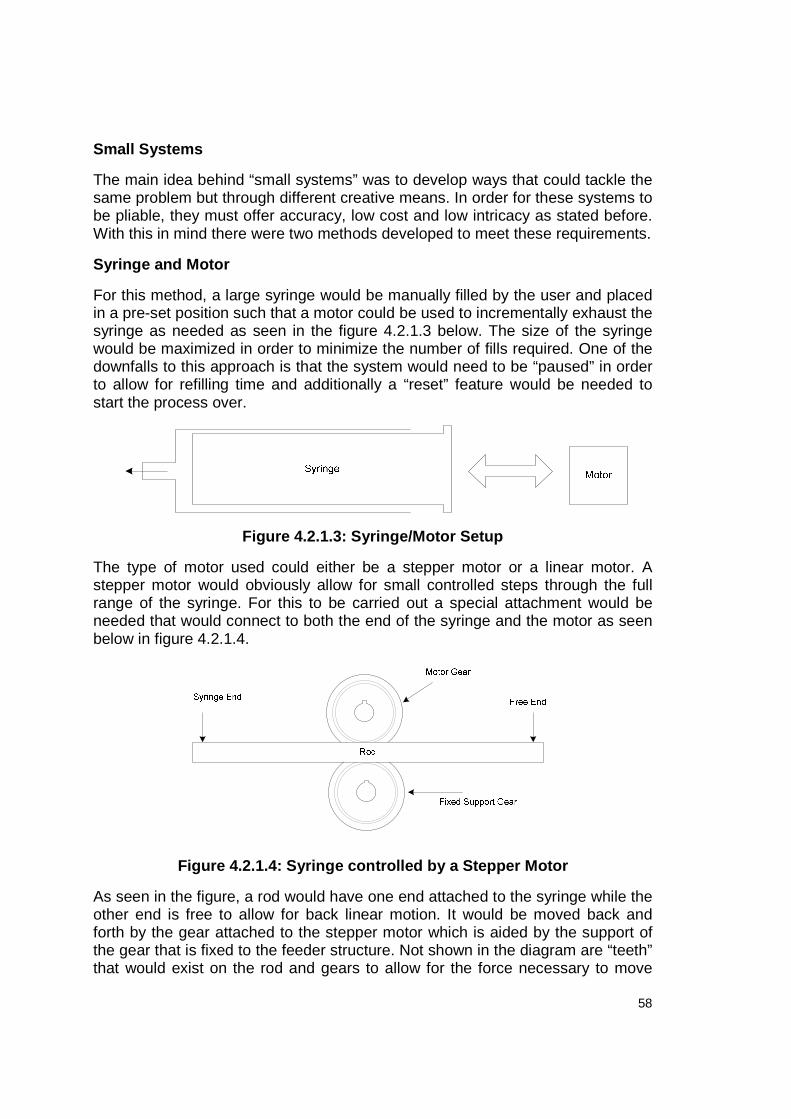
58

Small Systems

The main idea behind “small systems” was to develop ways that could tackle the same problem but through different creative means. In order for these systems to be pliable, they must offer accuracy, low cost and low intricacy as stated before. With this in mind there were two methods developed to meet these requirements.

Syringe and Motor

For this method, a large syringe would be manually filled by the user and placed in a pre-set position such that a motor could be used to incrementally exhaust the syringe as needed as seen in the figure 4.2.1.3 below. The size of the syringe would be maximized in order to minimize the number of fills required. One of the downfalls to this approach is that the system would need to be “paused” in order to allow for refilling time and additionally a “reset” feature would be needed to start the process over.

Figure 4.2.1.3: Syringe/Motor Setup

The type of motor used could either be a stepper motor or a linear motor. A stepper motor would obviously allow for small controlled steps through the full range of the syringe. For this to be carried out a special attachment would be needed that would connect to both the end of the syringe and the motor as seen below in figure 4.2.1.4.

Figure 4.2.1.4: Syringe controlled by a Stepper Mot or

As seen in the figure, a rod would have one end attached to the syringe while the other end is free to allow for back linear motion. It would be moved back and forth by the gear attached to the stepper motor which is aided by the support of the gear that is fixed to the feeder structure. Not shown in the diagram are “teeth” that would exist on the rod and gears to allow for the force necessary to move

59

the rod. Alternatively, the same rod can be attached to a linear motor that would allow for the same kind of motion.

Peristaltic Pump

A peristaltic pump is an existing type of pump that can distribute liquid in small doses at controlled rates and does not require any external pressure to be added to the system to operate. In practice, there exist multiple variations of this type of pump and for almost all cases the cost can be tremendous to purchase, especially when three of them are needed. To avoid the high cost of purchasing these types of pumps, it was proposed that the same process be created from existing parts.

Figure 4.2.1.5 Peristaltic Pump

The above figure shows the basic setup of such a pump. The main components consist of a disk with evenly spaced pegs extruding from it. Starting from one side of the support, silicon tubing is routed up through a hole and stretched around the pegs such that the pegs act as barriers by compressing the tube and allow a small space for liquid to be stored. As the disk is rotated, the pocket of liquid remains constant and exits out the other side. As the pump continues this process, liquid is continuously filled into these discrete pockets by creating its own pressure and drawing liquid from a reservoir. The idea control for this type of setup would be a stepper motor which allows for precise turns of the disk.

Component Selection

In order to minimize cost and employ a device that gives the precision flow required in this project, it has been decided that peristaltic type pumps is used. However, because these pumps are quite expensive when purchased direct from manufacturers, they have instead been made from general parts. In fact, a DIY

60

website19 was found that laid out a foundation for building such a device and a rough photograph can be seen in the picture below.

Figure 4.2.1.6: Photograph of Homemade Peristaltic Pump Permission requested from Divvy von Testa

The photograph shows the peristaltic pump made out of materials such as a kitchen timer, screws with pieces of nylon tubing, intravenous tubing and has been mounted on some door hinge brackets. For the purpose of this project, stepper motors is employed using the gears inside the timer to turn the dial. It can also be seen from the photograph that the amount of liquid that is passed through is dependent on the spacing between the screws. For this project, the distance between the screws must be small enough to provide the correct amount of fluid. At this point it is hard to define any actual characteristics of the pump as they is determined while the device is being built and tested.

Implementation

It was decided that at no point and time would any of the motors be running simultaneously, therefore in order to maximize the outputs of the microcontroller all three pump motors is powered using a signal from a de-multiplexer which is controlled by the microcontroller. In this configuration the motors would actually be on the same multiplexer as other components which would also not need to be controlled simultaneously. Because stepper motors is used for the rotation of the pump, a stepper driver circuit is needed just as it had been required with the lighting system. In fact, a similar circuit is employed, however the control of the motor is simplified based on the characteristics of its use. Meaning, it only needs to travel in one direction, it only operates in half stepping mode, the enable ability

19

http://translate.google.com/translate?prev=hp&hl=en&js=n&u=http://www.home.zonnet.nl/rsetteur/a

quarium/karel/doseer_pmp/index_doseer.htm%0D%0A%0D%0A&sl=nl&tl=en

61

is controlled by a de-multiplexer and it does not have the additional HOME and RESET control features. One additional feature that is implemented is the ability of the driver circuits to slave off of one main driver circuit which has the input of the RC oscillator. The configuration of the elements can be seen in the figure below.

Figure 4.2.1.7: Stepper Motor Control Configuration for use in Regulation

Stepper Driver Circuit

As seen in the lighting system, the L297/298 driver setup seems to be the best option at this point as it can provide the full range of voltage and current to operate the chosen stepper motor. The schematic below in Figure 4.2.1.8 shows the general configuration for the regulation system. One additional feature that is used in this setup that was not used previously in the lighting system is the use of OSC feature. This allows for the use of a single RC oscillator to be connected to one of the driver circuits while the others can use the SYNC feature so that they share the same signal.

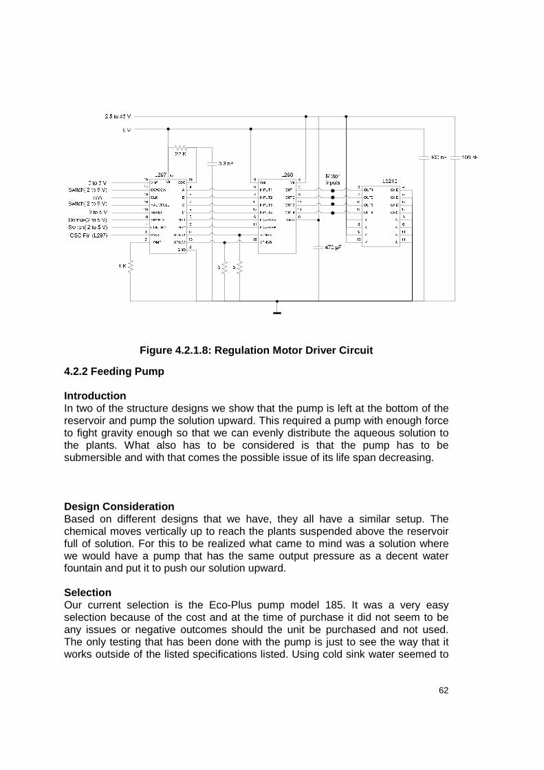
62

Figure 4.2.1.8: Regulation Motor Driver Circuit

4.2.2 Feeding Pump Introduction In two of the structure designs we show that the pump is left at the bottom of the reservoir and pump the solution upward. This required a pump with enough force to fight gravity enough so that we can evenly distribute the aqueous solution to the plants. What also has to be considered is that the pump has to be submersible and with that comes the possible issue of its life span decreasing. Design Consideration Based on different designs that we have, they all have a similar setup. The chemical moves vertically up to reach the plants suspended above the reservoir full of solution. For this to be realized what came to mind was a solution where we would have a pump that has the same output pressure as a decent water fountain and put it to push our solution upward. Selection Our current selection is the Eco-Plus pump model 185. It was a very easy selection because of the cost and at the time of purchase it did not seem to be any issues or negative outcomes should the unit be purchased and not used. The only testing that has been done with the pump is just to see the way that it works outside of the listed specifications listed. Using cold sink water seemed to

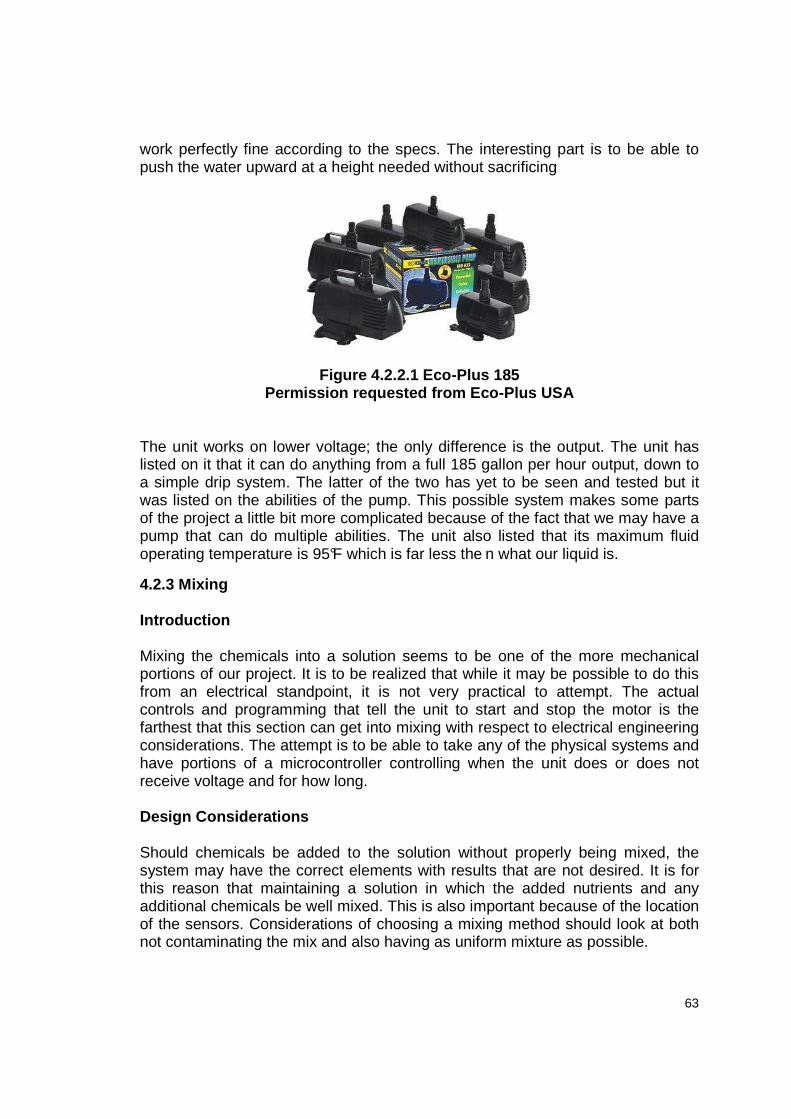
63

work perfectly fine according to the specs. The interesting part is to be able to push the water upward at a height needed without sacrificing

Figure 4.2.2.1 Eco-Plus 185

Permission requested from Eco-Plus USA The unit works on lower voltage; the only difference is the output. The unit has listed on it that it can do anything from a full 185 gallon per hour output, down to a simple drip system. The latter of the two has yet to be seen and tested but it was listed on the abilities of the pump. This possible system makes some parts of the project a little bit more complicated because of the fact that we may have a pump that can do multiple abilities. The unit also listed that its maximum fluid operating temperature is 95°F which is far less the n what our liquid is.

4.2.3 Mixing Introduction Mixing the chemicals into a solution seems to be one of the more mechanical portions of our project. It is to be realized that while it may be possible to do this from an electrical standpoint, it is not very practical to attempt. The actual controls and programming that tell the unit to start and stop the motor is the farthest that this section can get into mixing with respect to electrical engineering considerations. The attempt is to be able to take any of the physical systems and have portions of a microcontroller controlling when the unit does or does not receive voltage and for how long. Design Considerations Should chemicals be added to the solution without properly being mixed, the system may have the correct elements with results that are not desired. It is for this reason that maintaining a solution in which the added nutrients and any additional chemicals be well mixed. This is also important because of the location of the sensors. Considerations of choosing a mixing method should look at both not contaminating the mix and also having as uniform mixture as possible.

64

Air In larger water management systems, one of the common methods in thoroughly mixing a solution is air. Attempting to mix a large solution with high pressure air input usually gives an even distribution throughout the reservoir. It is the combination of high pressure over an area that makes this method work well. For the design aspect it is to be noted that it would require minimal structure influence and greater interest be directed to correct pressure input. The system should be outside of the water with one input into the solution. As long as it is raised high enough from the solution level, water back feeding into the air pump should not be an issue. This system has very little in it that can influence they results negatively. As long as it is turned on for a decent calculated amount of time then it should work to mix the solution without contaminating the chemicals, given that the air that it uses as input has as little impurities as possible. Fan Getting a well blend of a solution with a physical fan or blade is a very common approach when mixing is the issue. One of the issues that this method is subject to is the amount of this method that deals with mechanical aspects. Water Cycling There are several pumps on the market which come with specific connections for cycling water to itself; the only issue is the structure of this system may leave the solution at levels where not all the chemicals get mixed properly. This is not to say that it cannot get done, it just leaves portions of this method to be calculated with more variables, such as location of the intake and output tubing. With that said, it is also important to note that if you have an external pumping system it has to be maintained so that the external tubing does not form any leaks which can be devastating to the reservoir. Seeing as how most of these mixtures are teaspoons to the gallon, it is simple to get bad readings on sensors should the correct amount of chemical is not dispersed through the system. The only reason why this is more critical to this method is due to the fact that most of these pump methods require there to be water at that input valve. One of the concerns when attempting to implement this method is the portions of mixture left in sections of the tubing. Component Selection After considering the theoretical cost and integration to the project, the group has decided to go with an Air design. This design would have high pressured air blowing into the reservoir and would make it so that the solution would mix relative to that point. If during testing, the mix is not blending enough with one pump, a possible fix to this would be adding additional air pump inputs because of the low cost to the project. What is good about this method is that because of

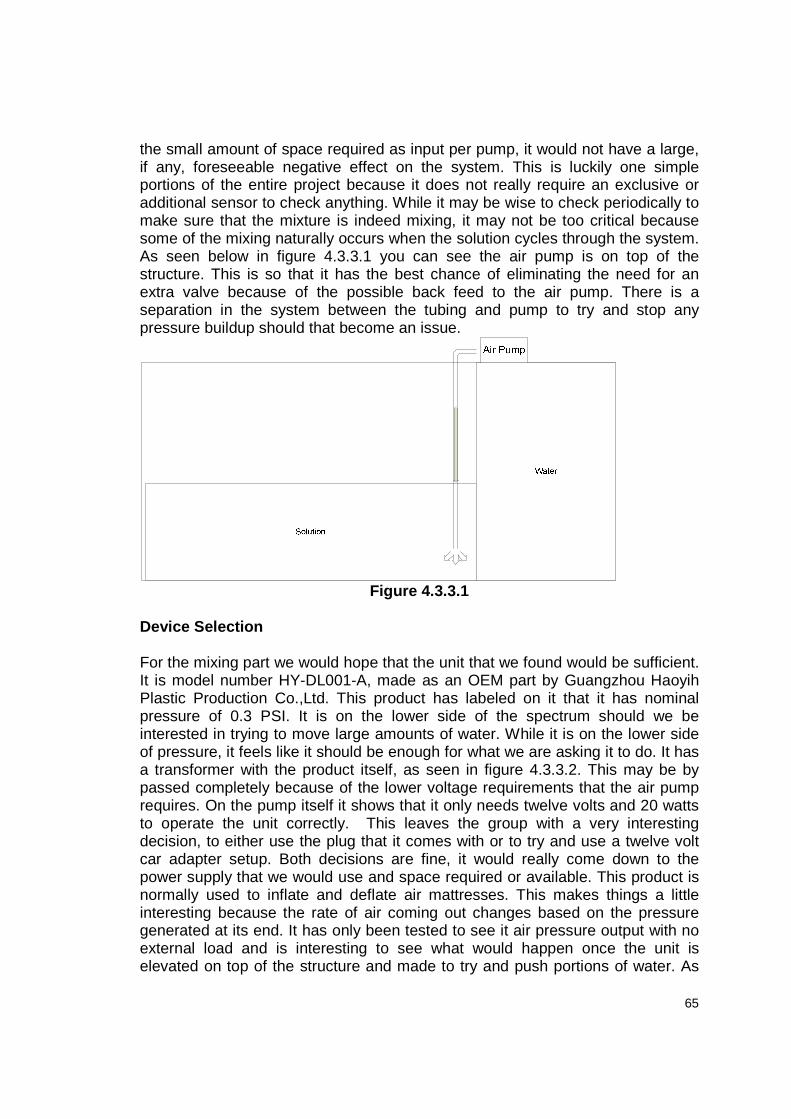
65

the small amount of space required as input per pump, it would not have a large, if any, foreseeable negative effect on the system. This is luckily one simple portions of the entire project because it does not really require an exclusive or additional sensor to check anything. While it may be wise to check periodically to make sure that the mixture is indeed mixing, it may not be too critical because some of the mixing naturally occurs when the solution cycles through the system. As seen below in figure 4.3.3.1 you can see the air pump is on top of the structure. This is so that it has the best chance of eliminating the need for an extra valve because of the possible back feed to the air pump. There is a separation in the system between the tubing and pump to try and stop any pressure buildup should that become an issue.

Figure 4.3.3.1

Device Selection For the mixing part we would hope that the unit that we found would be sufficient. It is model number HY-DL001-A, made as an OEM part by Guangzhou Haoyih Plastic Production Co.,Ltd. This product has labeled on it that it has nominal pressure of 0.3 PSI. It is on the lower side of the spectrum should we be interested in trying to move large amounts of water. While it is on the lower side of pressure, it feels like it should be enough for what we are asking it to do. It has a transformer with the product itself, as seen in figure 4.3.3.2. This may be by passed completely because of the lower voltage requirements that the air pump requires. On the pump itself it shows that it only needs twelve volts and 20 watts to operate the unit correctly. This leaves the group with a very interesting decision, to either use the plug that it comes with or to try and use a twelve volt car adapter setup. Both decisions are fine, it would really come down to the power supply that we would use and space required or available. This product is normally used to inflate and deflate air mattresses. This makes things a little interesting because the rate of air coming out changes based on the pressure generated at its end. It has only been tested to see it air pressure output with no external load and is interesting to see what would happen once the unit is elevated on top of the structure and made to try and push portions of water. As

66

mentioned above should the one air pump not be sufficient, the idea would be to try and use multiple pumps. The only problem that seems to be present is that this was something that was around the house and it seems to be a little difficult to get an additional pump. It would be more convenient to get a pump with similar specifications to add it to the setup and have multiple inputs. It would actually start to make more sense to try and get just one larger, higher pressured pump to get the job done correctly instead of getting similar weak pumps.

Figure 4.3.3.2 Permission Requested from Guangzhou Haoyih Plastic Production Co.,Ltd

67

Chapter 5: Power System Introduction

For this project, a dynamic range of power is distributed throughout the system where components such as the lighting, valves and pumps require AC power while all others require DC power. It is required that the system as a whole be powered by a single AC input from standard wall outlet, therefore the AC needs to be converted to DC as well as distributed amongst those elements that require AC. The range of the DC components require a maximum of 50 V overall and the range of the AC components require 120 VAC and 24 VAC. The block diagram below outlines the configuration of the power distribution:

Figure 5.0.1: Power System Configuration

As it can be seen in the figure above, the 120 VAC is split into three separate divisions: AC/DC, AC/AC and 120 VAC. The AC/DC is used to provide power for the various digital circuitries throughout the system; the AC/AC is only used to power the valves; and the 120 VAC runs straight through to the necessary components requiring this voltage. Additionally, all of the AC components need to be connected to relays for on/off switching controlled by the microcontroller.

5.1 AC/DC and AC/AC Conversion The obvious goal of the AC/DC and AC/AC converter is to step down the input voltage of 120 VACrms to the required voltage. For the AC/DC converter a maximum output of 50 VDC is required as this is the maximum range of the

68

motors. However, at this point in the project it is unknown what the exact voltage is that is used with the motors which depend on how well they perform under their given conditions. During the testing of the motors, a lower voltage of 5 V is used initially and is increased as needed; thus at this point the maximum draw is assumed for this design. After searching for powered supplies that may initially meet our needs, it was decided that it was necessary to design the AC/DC converter since finding a power supply rated at the needed voltage can be expensive.

Figure 5.1.1: AC/DC Power Conversion

As shown in Figure 5.1.1, the input voltage is stepped down through the transformer and then rectified using the Full Wave Bridge Rectifier. The transformer has a turn ratio of 10:3 which allows the transformer to step down from 120 VACrms to a peak AC value of 48 V. The output is then connected to an RC filter with a large enough time constant to reduce the ripple effects significantly. The output of this particular setup is approximately 48 VDC. The maximum current ratings for the components should be around 5 to 10 Amps of which the precise number is determined at a later time.

The AC/AC converter should provide a single output of 24 VACrms, which is the necessary voltage required by the valves. As with the AC/DC converter, since the power supply is not the main focus of this project, if the AC/AC converter has been purchased. The design of the AC/AC converter can be seen below:

Figure 5.1.2: AC/AC Power Conversion

D1

3N256

1

2

4

3

V1

120 Vrms 60 Hz 0°

GND

C1500uF

T1

2

34

GND

R220kΩ

0

1

10:3

Probe3,Probe1

V: 47.9 V I: 7.57 mA

V2

120 Vrms 60 Hz 0°

GND

T2

5

GND

R11kΩ

0

6

5:1

Probe4,Probe2

V(p-p): 67.8 V V(rms): 24.0 V V(dc): -161 uV Freq.: 60.0 Hz

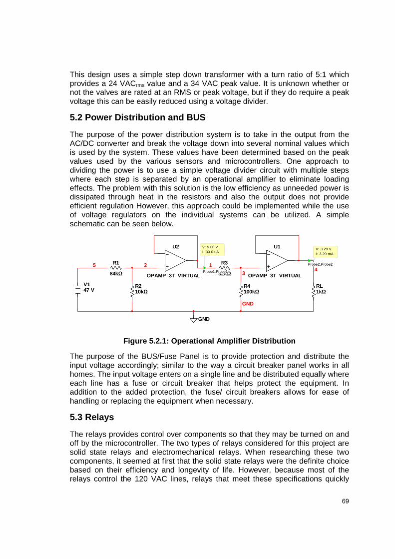
69

This design uses a simple step down transformer with a turn ratio of 5:1 which provides a 24 VACrms value and a 34 VAC peak value. It is unknown whether or not the valves are rated at an RMS or peak voltage, but if they do require a peak voltage this can be easily reduced using a voltage divider.

5.2 Power Distribution and BUS The purpose of the power distribution system is to take in the output from the AC/DC converter and break the voltage down into several nominal values which is used by the system. These values have been determined based on the peak values used by the various sensors and microcontrollers. One approach to dividing the power is to use a simple voltage divider circuit with multiple steps where each step is separated by an operational amplifier to eliminate loading effects. The problem with this solution is the low efficiency as unneeded power is dissipated through heat in the resistors and also the output does not provide efficient regulation However, this approach could be implemented while the use of voltage regulators on the individual systems can be utilized. A simple schematic can be seen below.

Figure 5.2.1: Operational Amplifier Distribution

The purpose of the BUS/Fuse Panel is to provide protection and distribute the input voltage accordingly; similar to the way a circuit breaker panel works in all homes. The input voltage enters on a single line and be distributed equally where each line has a fuse or circuit breaker that helps protect the equipment. In addition to the added protection, the fuse/ circuit breakers allows for ease of handling or replacing the equipment when necessary.

5.3 Relays The relays provides control over components so that they may be turned on and off by the microcontroller. The two types of relays considered for this project are solid state relays and electromechanical relays. When researching these two components, it seemed at first that the solid state relays were the definite choice based on their efficiency and longevity of life. However, because most of the relays control the 120 VAC lines, relays that meet these specifications quickly

U2

OPAMP_3T_VIRTUAL

R1

84kΩ

GND

V147 V

R210kΩ

R3

52kΩ

R4100kΩ

U1

OPAMP_3T_VIRTUAL

2

3

5 1

RL1kΩ

GND

4Probe1,Probe1

V: 5.00 V I: 33.0 uA

Probe2,Probe2

V: 3.29 V I: 3.29 mA

70

become expensive costing around $20 or more. Since we would need five of them we would have to spend $100 on relays alone which is far too much for this operation. Knowing this, the electro-mechanical relays then seemed to be the next best solution. The only real down fall to the electromechanical relays is their life span, but at a quarter of the cost of the solid state relays this would not be an issue.

71

Chapter 6: Structure

6.1 Structure Methods Introduction The structure of the system itself is still in the planning stages. It currently is between a couple different design options as sensors and additional parts become available. The overall design has been chosen to be a rectangular, thinner shaped system as opposed to the dome design as originally specified. This was decided upon because of the simplicity and the expansion that this type of system can offer, should it be necessary in the future. Design Considerations The designs that are under consideration are systems that use the idea of the Ebb and Flow as well as Flood and Drain hydroponics systems. The designs would use pumps to send the solution through each of the plants roots for a specified amount of time, multiple times per day as needed. The structure itself would be holding both the electrical components and the various chemical solutions in single structure, without the need for anything to be mounted in a remote location. Structure A This design is currently not portraying the lighting solution because the lighting system is under review by the group, trying to determine the intensity of the mechanical aspect of an automated lighting system. Because the rest of the motors, chemicals and tubing are inclusive, it would be ideal to incorporate a lighting system that plays into the structure, making it as inconspicuous as possible as seen in figure 6.1.1a and b below. This structure has a starting point at the water reservoir, with it as well as the other chemical solutions being filled at a maximum and the solution tank as empty as possible. This would portray the water cycling process, which would occur any time we estimate to be necessary for the solution to be flushed out and a new mixture be added, usually on a two week interval. Multiple employees from the Sunshine hydroponics store have mentioned that a usual period that goes by that would be good to change the water is about a week or two for small to medium plants and shorter time as the size of the plant increases. From an empty solution reservoir, the initial liquid to be added should be the water. The system has a liquid level sensor and being that an amount of liquid going in has been preset; the amount of nutrients needed can be proportioned out and added into the water that is being held in the solution tank. At this point should be a wise decision to capture the levels of pH and nutrient concentration in our system. By doing it at this point, it can be shown that there is no acidic contamination in the

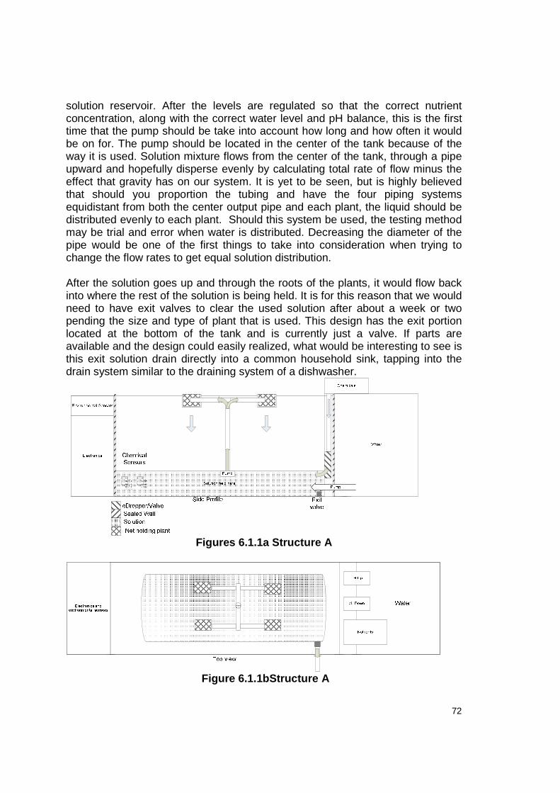
72

solution reservoir. After the levels are regulated so that the correct nutrient concentration, along with the correct water level and pH balance, this is the first time that the pump should be take into account how long and how often it would be on for. The pump should be located in the center of the tank because of the way it is used. Solution mixture flows from the center of the tank, through a pipe upward and hopefully disperse evenly by calculating total rate of flow minus the effect that gravity has on our system. It is yet to be seen, but is highly believed that should you proportion the tubing and have the four piping systems equidistant from both the center output pipe and each plant, the liquid should be distributed evenly to each plant. Should this system be used, the testing method may be trial and error when water is distributed. Decreasing the diameter of the pipe would be one of the first things to take into consideration when trying to change the flow rates to get equal solution distribution. After the solution goes up and through the roots of the plants, it would flow back into where the rest of the solution is being held. It is for this reason that we would need to have exit valves to clear the used solution after about a week or two pending the size and type of plant that is used. This design has the exit portion located at the bottom of the tank and is currently just a valve. If parts are available and the design could easily realized, what would be interesting to see is this exit solution drain directly into a common household sink, tapping into the drain system similar to the draining system of a dishwasher.

Figures 6.1.1a Structure A

Figure 6.1.1bStructure A

73

Structure B The major differences between this system and the previous are that this has incorporated the lighting into the structure by the use of an adjustable pole. The same basic principles apply to this structure; the initial state with full chemical liquids with an empty solution reservoir ready either from first use or just after the system has been determined that it needs a new solution mixture. Another major difference should be noted when looking at where the old solution is being placed. With this system you are able to save the used liquids. When looking at the greater scheme of things it can be seen that this system is not restricted by location as the first design is. By not needing to have it connected to a draining system it gives the user more locations to use an automated hydroponics system.

Ad

justa

ble

Po

le

Figure 6.1.2 Structure B

One of the final notes that is important to mention about this setup is the fact that it not only uses a flood and drain system, but it is also currently being looked into ways on how to design a tray that would hold the plant and would allow the use of a water culture hydroponic system. This would ideally start with the plants being suspended at the top of the solution tank with no contact with the solution. When the pumps are turned on, the tray feeds the liquids to our plants as the previous Ebb and Flow systems were working with the exception that it would be a water collection process as oppose to having an open port allowing the liquids to flow out. After a given amount of time the liquid would then drain out of the tray and would go back to where the rest of the solution is being held. If the try was

74

constantly being cycled from the used portions to the portions of the solution that are not being used, then that would give the plant the effect that it is always in the water, taking as much as nutrients as it can without being restricted to a time limit of when it can take its chemicals. It was explained to the group that there is a company that tries to use a hydroponic system that does not reuse the nutrients, but rather have a constant stream of the mixture going to the plants at all times. In those trials, the plants grew at significantly larger rates then most hydroponic systems which already boast a large production cycle. It is this thought process that make a person wonder at the possibilities of output by trying to overfeed a plant Structure C

Solution

Pump

Valve

Mesh Net

Lighting

Figure 6.1.3 Structure C

The final consideration is shown above in figure 6.1.3. This is a very compact and efficient model which has the design consideration where there would be a direct feed into the reservoir itself. This system removes the tank where the water used to be held and rather replaces that with a hose, either from the garden, or the kitchen sink. By doing this, it makes the system a smaller dimension so that it is easier to transport however it does make it so that the end user has to be near a hose if it is to be automated. The good part of this is the fact that it should only be about once every two weeks or so that the water is input into the tank. If plugging it in every two weeks does not seem to be such a large of an issue, then this might be the ideal case. That is also keeping in mind that the changes in pH or the nutrient concentration does not vary much so that any additional water

75

does not have to be used. On the bottom and the right of the structure is shown a valve. This valve is here so that pressure can be maintained at the ends and still allow there to be no change to the system. The valve that the group is currently considering is shown in figure 6.1.4 which is the Hunter 1": PGV-100G-S valve. It is available in four 1" body configurations, in either an angle, globe, male by male, male by barb design. While it is rated at 150 psi, the project only uses it as a switch that either gravity or a hose is supplying, which is less than the pressure that this can withstand. The unit list that its operating pressures are from 20 to 150 psi and we is on the lower end of those specifications. What is beneficial to the project is the flow rates and the small amount that is able to be achieved by this pump which ranges from .2 to 120 gallons per minute. This may turn out to be more useful than just a flood and drain pump because of the small inputs that it can achieve. The only reason why it cannot do it all is because of the required pressure that it needs at its ends to function. Based on the allowed flow rates, what would be a reasonable input could be something around two gallons a minute. This setting would be because the reservoir would be around 10 gallons. There is no need to fill it at any specific value so it does not matter what rate is chosen, just as long as it is at an acceptable rate for the user. The system seems to have just an on and off function and its flow rate is set externally as oppose to the supplied voltage like other portions of the project.

Figure 6.1.4 Hunter PVG Valve

Permission requested from Hunter Irrigation 6.2 Sensors Chemical Sensors The chemical sensors are in positions that would allow constant/on-demand measurements of the quantity of each in the solution. As the plant is fed the chemical make-up of the solution changes based on the amount of nutrients that the plant will consume. This feeding cycle, over time reduces the amount of each chemical because the used, non-consumed portion is being put back into the solution reservoir. Once the quantities have reached a given a minimum threshold they would be replenished accordingly through a small dropper

76

solution. These sensors has digital outputs only and this information is used at our systems discretion to adjust accordingly through database or the users web interface. A problem has been brought up by one of the sales associates of the company HM Digital. They bring up the point where it may not be in the group’s best interest to use certain portable handheld meters when trying to permanently affix these sensors onto a structure. It has been expressed that there are specific product that has these capabilities, or at least better suited when trying to get a constant output to let you know the concentration of certain chemical aspects of this project. This has been debated since the issue was brought up, if it should be considered to follow the advice given or to try and pass on the advice and do as pleased. The only real concrete piece of information given was that they do indeed sell meters that are made to stay on for indefinite amount of time. This brings up the question as to why there has been a sense that there is information being withheld, such as to what test data shows the recommended maximum amount of time that the units can be left in a solution. Environmental Sensors As long as the sensors are in close proximity with the actual plants themselves, it does not make much of a difference as to their physical position. For aesthetic purposes, it would be well placed on top of the electrical components and to the side of the plants. The sensors would include lighting, CO2, humidity and temperature. Each has its independent microcontroller that would take that physical data and pass information online. At this stage of the project there are no intentions to try and adjust these parameters but are more so there for read only features to notify the user or for climate changes and what effect that has on the plants. Liquid Level Sensor This portion of the project has been left currently off because of pending design considerations based on the type of sensor that shall be implemented. This sensor allows tracking of the liquid so that the correct pH and nutrient solutions can be added to the system, as they are proportional to the amount of water in the system. While it may not be as critical to decide on an actual sensor, knowing the exact amount of water with is critical to measurements. All three chemical solutions is highly dependent on the level of solution because of the nature of the chemicals themselves. The size of the system is actually large enough so that even though we may have a drop or two more then the recipe calls for, the total diluted solution should be large enough so that there can be a relatively large percentage error and still be well within a reasonable range for the plants.

77

6.3 Lighting The lighting portion of the project has been left currently off because of pending design considerations based on electrical vs. mechanical implementation. The lighting system is critical to a plants health and is implemented with practicality in mind. The only part of the lighting system which is concrete at this time is the fact that it is suspended by our setup as opposed to be a fixture that is hung or a standing light setup. The second model actually incorporates this fixture in the system itself by having a manual light level. There is nothing wrong with this manner and pending cost of the rest of the system might end up being the type of setup we would go with. A recent idea came up where there would be a pulley system setup which would raise the entire fixture based on the height of the plant. By using a type of infrared sensor we can track the height of the plant and automatically raise the fixture once the plant crosses certain boundaries, commonly seen in garage door safety systems. 6.4 Frame and Electronics Protection The frame is sturdy enough to more than compensate for the fact that this entire unit moves more than a few times. There are several liquids which need small portions to be added into our system which is to say that rigidity is essential in these portions of the frame. While it is great to have an almost immoveable frame, the weight usually increases with a firm design. It is seen in each design consideration that the electrical components have been carefully separated from any liquids. Given normal usage, it is unnecessary to try and spec out certain situations for highly improbable situations. The electronics is close to the liquids which makes any electrical engineer a little sensitive to the thought as to what might happen should there be a leak in the system. Currently there are no situations that are deemed critical enough as to move the entire electrical components away from the liquids. At most it was foreseen that the entire boards were both covered in a case and wrapped for a random chance of spillage. A final thought to note is the height of the components themselves. Should they be at a high enough height, in the event of a leak in the reservoirs should not be enough liquid to reach the level that can do any serious damage. 6.5 Piping The structure itself requires at least two different types of piping. The solution and the chemical components have two different volumes and flow rates, requiring the difference in sizes of the tubing. While it may be possible to use the same size, it may not be as practical to dilute the chemicals so that the system has equal pipes flowing liquids throughout. In the feeding portion of the project, to allow for even water flow, the solutions pipes have been routed in such a fashion as to allow for even liquid dispersion. In the regulation portion of the project, the chemical solution requires a smaller amount of liquid, possibly in the order of an eighth inch plastic tubing. These small measurements that cause us to consider

78

solutions that have been used in the medical field for some time now. Regardless if an automated syringe is used or a system where a regulated IV machine is used the volume of the liquid remains the same. 6.6 Reservoirs The system itself requires at minimum five reservoirs holding the pH up and down, Nutrients, water, and the mixture itself. Depending on what type of cycling is used an additional holder may be required to the used output like in the second structure. Luckily three of these chemicals only require minimal amounts to be added to our solution, something in the order of a teaspoon per gallon. It is very easily and inexpensive to acquire a liters worth of these chemicals possibly out living the actual plant itself. While it is to be taken into account the fact that there are multiple plants, and with each plant it increases the consumption of the chemicals, it still almost seems negligible when looking at the entire system and the need to compensate for the changes per plant that it is going to have. The only thing that should be carefully watched is the fact that plants can get infected which can radically change the chemical solution. Should one of the plants in the system get infected and output large amounts of acid into our system, our system would be programmed to compensate for the increase in acid by adding the pH down solution. If only one is infected changing the makeup of the solution and the other plants are still requiring a higher pH balance the entire cycle could be compromised and the batch can most likely die without chance of salvation if not caught soon enough. This is currently being resolved by constantly tracking the balances of both the chemical elements and the environmental elements to try and minimize the possibility of improper growth as well as hazardous ranges of the entire system. Water Tank The tank which holds the reserve water should be built so that sufficient amount of water is in there so that it gives plenty of time before refill occurs. It may even be a possibility that instead of a tank, a hose is directly connected to the input and an electronic valve controls as shown above in figure 6.1.4. When and how much is actually input into the solution is then solely controlled by an electronic valve or something to that effect. If there is a stationary tank at the solution input, the only time this needs to be filled is for a theoretical time where you have the automated system take over. For testing portions, it only needed to be partially filled. Considering the size of the tank, it was a feasible solution to have a detachable water reservoir so that a tank or a water hose can be connected. The actual mineral components in the input water are not as critical to the system as the nutrients are. It is for this reason that any type of water, with the exception of contaminated water, is perfectly able to be used in the system. There are some exceptions to this because of the way that certain chemicals react in certain solutions. In section 2.6 it is listed in the design considerations what possible

79

outcomes of different types of water use has on the overall plant growth. In general, it is not a wise idea to try and use fancy water, the more natural the source the better the function is and the plant is able to adapt to it.

80

Chapter 7: Build

7.1 Group Responsibilities The various parts of the project have been divided based on the engineering background of the different group members. Since the group consists of two electrical engineers and one computer engineer, each member takes a part in accordance with their major. However, the division of these sections does not necessarily imply that each member has solely been doing these sections alone, but the responsibility for the sections is headed by those group members. Additionally, not all parts is completely headed by a single group member, but is evenly carried out by all group members. The table below outlines the division of the responsibility of parts amongst group members:

Section Lead Lighting System Doug Cooper Sensors Doug Cooper Regulation System Sam Reyna Power System Sam Reyna Wireless Interface Desmond Persaud Database Desmond Persaud Structure No Lead

Table 7.1: Group Responsibilities

7.2 Project Schedule The project schedules for Senior Design 1 and 2 are estimations of where the project should be at the given dates. These estimations are based on the timeframes in which each part “should” take, more or less. The majority of the schedule for Senior Design 1 was given to the research portion of the project. During this time there are many unknowns that must be figured out and therefore extra time was given to this area to meet the deadlines. While doing the research, each member was expected document their designated portions of the document accordingly. Once the research phase was completed, the remaining time was devoted to design and finalizing the documentation. Senior Design 2 posed a bit more of a difficult task especially when trying to meet deadlines that were unknown at the time of the writing of this documentation. As a result, the dates were moved to as early a deadline as possible so as to meet the unknown deadlines which would definitely be towards the end of the semester. The sequence of the schedule was designed such that each event happens in a sequence where one must come before the next.

81

Task Name Duration Start Finish Senior Design 1 64 days 1/29/2009 4/27/2009

Determine Project Idea 1 days 2/6/2009 2/6/2009 Initial Project and Group Identification

Document 0 days 1/29/2009 1/29/2009 Determine New Project Idea 8 days 2/2/2009 2/11/2009 Turn in new Project Idea 0 days 2/12/2009 2/12/2009 Table of Contents Due 0 days 2/24/2009 2/24/2009 Research 13 days 2/25/2009 3/13/2009

Desmond to Research Wireless Connectivity, MCU's 13 days 2/25/2009 3/13/2009

Doug to Research CO2, Humidity, Temp, Liquid Level Sensors 13 days 2/25/2009 3/13/2009

Sam to research pH, Conductivity, Water Mixing 13 days 2/25/2009 3/13/2009

10 Pages Completed per person 0 days 3/13/2009 3/13/2009 Continue Research 21 days 3/16/2009 4/10/2009

Desmond to Research external storage, web interface, database 20 days 3/17/2009 4/10/2009 Doug to Research Lighting, Chemical

Dispersion 10 days 3/16/2009 3/27/2009 Sam to Research Structure, Water

Dispersion 10 days 3/16/2009 3/27/2009 10 Pages Completed per person 9 days 3/27/2009 4/7/2009 Finalize components to be used in

project/Order Components 1 days 4/9/2009 4/9/2009 Design electrical system 6 days 4/10/2009 4/17/2009 Develop Testing Procedures 3 days 4/18/2009 4/21/2009 Finalize Executive Summary 3 days 4/18/2009 4/21/2009 30 Pages Completed 0 days 4/21/2009 4/21/2009 Format and Print Documentation 4 days 4/1/2009 4/4/2009 Initial Project Documentation Due 0 days 4/28/2009 4/28/2009

Task Name Duration Start Finish Senior Design 2 42 days 5/1/2009 6/26/2009

Build 24 days 5/1/2009 5/18/2009 Structure 24 days 5/4/2009 5/17/2009 Circuitry 24 days 5/18/2009 6/1/2009 Web Interface 24 days 5/18/2009 6/1/2009 Combining Components 24 days 6/2/2009 6/15/2009

Testing 12 days 6/16/2009 7/1/2009 Sensors 12 days 6/16/2009 6/22/2009 Pumps/Valves 12 days 6/23/2009 6/23/2009 Lighting 12 days 6/24/2009 7/1/2009

Testing/Troubleshooting 5 days 7/2/2009 7/7/2009 PCB Fabrications 1 days 7/8/2009 7/15/2009 Critical Design Review 1 days 7/16/2009 7/16/2009 Peer Review 1 days 7/20/2009 7/20/2009 Final Presentation and Demo 1 days 7/24/2009 7/24/2009

Table 7.2.1 Project Schedule

82

7.3 Bill of Materials The materials listed below consist of all the major components that this project is comprised of. Many of the smaller components such as resistors and capacitors were not included because they can be obtained at little to no cost at all from the Senior Design lab, or assuming the cost of reproduction, they could be ordered in bulk at little to no cost. The “Actual” costs are based on how much has come out pocket while accounting for those components that have already been donated. The “Retail” costs account for actual costs plus the cost of the donated parts. The “Reproduction” costs account for the retail costs minus any developmental kits that are required for hardware implementation. Environmental Sensors

Component Actual Retail Reproduction Manufacturer Supplier CO2 $0 $130 $130 SenseAir Manufacturer Humidity/Temp.

$30 $30 $30 Humirel Digikey

Pressure $0 $3 $3 STMicroelec. Manufacturer pH $25 $25 $25 HANNA eBaY Conductivity/TDS

$19 $19 $19 HM Digital The Science Company

Total $74 $207 $207 Table 7.3.1 Sensors

Lighting System

Component Actual Retail Reproduction Manufacturer Supplier LED Light $40 $40 $40 Unknown California

Nursery Optical Sensor (x2)

$24 $24 $24 Sharp SparkFun

Contact Sensor

$0 $10 $10 Cherry Corp Manufacturer

Motor $8 $8 $8 Lin Engineering eBay Microcontroller $4 $4 $4 Atmel Mouser Stepper Motor Components

$2 $6 $6 STMicroelectronics

Manufacturer

Hardware $10 $10 $10 Home Depot Home Depot Total $88 $102 $102

Table 7.3.2 Lighting Components

83

Physical Structure

Component Actual Retail Reproduction Manufacturer Supplier Frame $40 $40 $40 Home Depot Home Depot Small Reservoirs (x3)

$15 $15 $15 Zevro Wal-Mart

Medium Reservoirs (x3)

$30 $30 $30 Sterilite Wal-Mart

Waterproofing $10 $10 $10 Home Depot Home Depot Hardware $20 $20 $20 Home Depot Home Depot Hydro Rocks $5 $5 $5 Hydroton HydroponicGar

den Pots (x4) $4 $4 $4 Unknown eBaY

Total $134 $134 $134 Table 7.3.3 Structure Components

Controls

Component Actual Retail Reproduction Manufacturer Supplier Microcontroller $0 $4 $4 Atmel Friend Web Server module

$0 $90 $90 Lantronix Manufacturer

Web Server Dev. Kit

$0 $120 $0 Lantronix Manufacturer

Antenna $0 $6 $6 Lantronix Manufacturer Demux $1 $1 $1 National Semi. Mouser SD Breakout Board

$18 $18 $18 Sparkfun Sparkfun

SD Card $14 $14 $14 Best Buy Sandisk Arduino Dev Kit

$0 $30 $0 Arduino Friend

Total $33 $283 $133 Table 7.3.4 Control Components

Fluids Management

Component Actual Retail Reproduction Manufacturer Supplier Valves (x2) $36 $36 $36 Toro Home depot Feed Pump $13 $13 $13 Unknown Unknown Air Pump $20 $20 $20 Coleman Camping

Comfortably Motors (x3) $24 $24 $24 Lin Engineering eBay Timers (x3) $18 $18 $18 Taylor Amazon Tubing $20 $20 $20 Home Depot Home Depot Relays (x5) $50 $50 $50 Skycraft Skycraft

Total $191 $191 $191 Table 7.3.5 Fluid Management Components

84

PCB Manufacturing

Component Actual Retail Reproduction Manufacturer Supplier Main Board $50 $50 $50 PCBExpress PCBExpress Power Board $50 $50 $50 PCBExpress PCBExpress Lighting Board $20 $20 $20 Skycraft Skycraft CO2/Humidity/Sensor Board

$10 $10 $10 Skycraft Skycraft

Pressure Sensor Board

$10 $10 $10 Skycraft Skycraft

Total $140 $140 $140 Table 7.3.6 PCB Manufacturing

7.4 Budget and Financing The idea budget for this project was considered to be around $300 per person for a total maximum cost of $900. This cost was based on a worst case scenario where there are no donations and the entire project is paid for out of pocket. Based on the major components considered in the Bill of Materials and their associated costs, the overall actual cost ended up to be approximately $660 for a total cost of $220 per person. The retail cost amounted to approximately $1057 for an overall savings of $397 and a savings of $132 per person. Since it was made possible to reduce the cost of the project below budget, the goal for the cost of the project was considered an accomplishment. A summary can be seen in the table below.

Budget Retail Cost Actual Cost Savings Total $900 $1057 $660 $397 Total/Person $300 $352 $220 $132

Table 7.4.1: Cost vs. Savings

7.5 Design Summary These design methods were chosen from our research of the various components in the system and at this the project is used in the prototyping and construction of the plant feeder. This design summary describes in detail each of the major components of the system and will show block diagrams and schematics that drive each system accordingly.

85

Figure 7.5.1: System overview block diagram

The above diagram 7.5.1 depicts the main overview of the system showing the main connections between each of the components in this system. The heart of the system lies in the center of the block diagram that contains the main microcontroller which controls the interface between the user and the peripherals of the system. The second major system in the block diagram is the lighting system which also has its own microcontroller and locally controls the lighting, in addition it also adjusts its own height and control day and night cycles. Power System

Figure 7.5.2: Power System block diagram

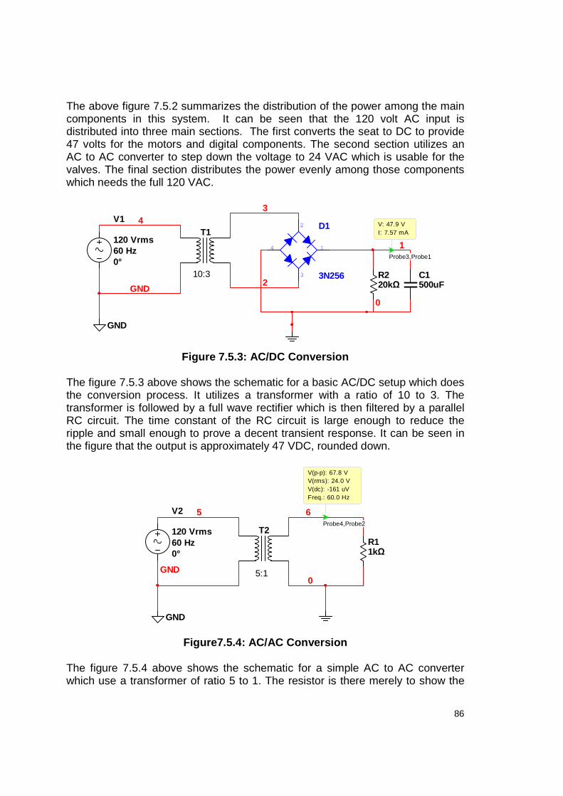
86

The above figure 7.5.2 summarizes the distribution of the power among the main components in this system. It can be seen that the 120 volt AC input is distributed into three main sections. The first converts the seat to DC to provide 47 volts for the motors and digital components. The second section utilizes an AC to AC converter to step down the voltage to 24 VAC which is usable for the valves. The final section distributes the power evenly among those components which needs the full 120 VAC.

Figure 7.5.3: AC/DC Conversion

The figure 7.5.3 above shows the schematic for a basic AC/DC setup which does the conversion process. It utilizes a transformer with a ratio of 10 to 3. The transformer is followed by a full wave rectifier which is then filtered by a parallel RC circuit. The time constant of the RC circuit is large enough to reduce the ripple and small enough to prove a decent transient response. It can be seen in the figure that the output is approximately 47 VDC, rounded down.

Figure7.5.4: AC/AC Conversion

The figure 7.5.4 above shows the schematic for a simple AC to AC converter which use a transformer of ratio 5 to 1. The resistor is there merely to show the

D1

3N256

1

2

4

3

V1

120 Vrms 60 Hz 0°

GND

C1500uF

T1

2

34

GND

R220kΩ

0

1

10:3

Probe3,Probe1

V: 47.9 V I: 7.57 mA

V2

120 Vrms 60 Hz 0°

GND

T2

5

GND

R11kΩ

0

6

5:1

Probe4,Probe2

V(p-p): 67.8 V V(rms): 24.0 V V(dc): -161 uV Freq.: 60.0 Hz

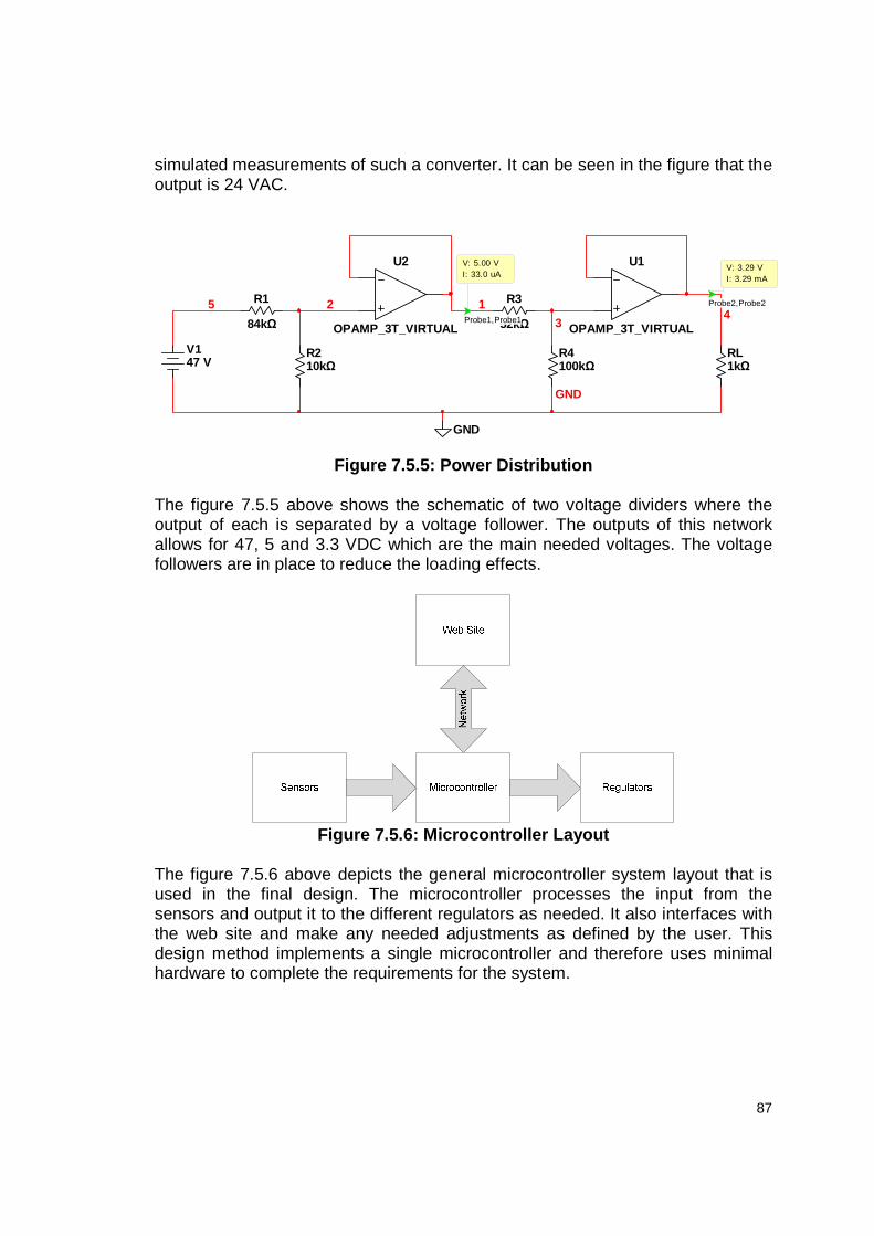
87

simulated measurements of such a converter. It can be seen in the figure that the output is 24 VAC.

Figure 7.5.5: Power Distribution

The figure 7.5.5 above shows the schematic of two voltage dividers where the output of each is separated by a voltage follower. The outputs of this network allows for 47, 5 and 3.3 VDC which are the main needed voltages. The voltage followers are in place to reduce the loading effects.

Figure 7.5.6: Microcontroller Layout

The figure 7.5.6 above depicts the general microcontroller system layout that is used in the final design. The microcontroller processes the input from the sensors and output it to the different regulators as needed. It also interfaces with the web site and make any needed adjustments as defined by the user. This design method implements a single microcontroller and therefore uses minimal hardware to complete the requirements for the system.

U2

OPAMP_3T_VIRTUAL

R1

84kΩ

GND

V147 V

R210kΩ

R3

52kΩ

R4100kΩ

U1

OPAMP_3T_VIRTUAL

2

3

5 1

RL1kΩ

GND

4Probe1,Probe1

V: 5.00 V I: 33.0 uA

Probe2,Probe2

V: 3.29 V I: 3.29 mA

88

Figure 7.5.7: Main Microcontroller Configuration

The figure above depicts the configuration of the main microcontroller. Five of the six analog to digital converts on the left side of the main microcontroller serve as inputs for the temperatures sensor, CO2 sensor, liquid level sensor, nutrient sensor and pH sensor respectively. The left side of the figure above shows the connection made by the microcontroller to the SD breakout board. It requires a few resistors to regulate the voltage for the input. The Rx and Tx lines above is used to communicate with the Lantronix module which in turn communicates with the internet and the website. The other lines are used for the controls system. A de-multiplexer is used to minimize the amount of outputs needed to control some of the regulators. Lighting System

Figure 7.5.8: Lighting System Operation

89

The figure above depicts the main concept of the lighting system operation. The basic concept is that the light self adjusts as the plants in the system grow taller. It utilizes an optical and contact sensor which provides feedback to the system. The optical sensor tells the system when an object is in its plane of sight while the contact sensor tells the system when the light has reached its maximum height. A stepper motor is used as the means in which to raise and lower the lighting.

Figure 7.5.9: Light Source Day/Night Configuration

The day and night cycle operation of the lighting system is accomplished using a relay which is controlled by the local microcontroller as seen in the figure above.

Figure 7.5.10: Light Source Motor Configuration

The stepper motor is controlled by a specialized driver circuit which controls both the power and rate at which the motor turns. The basic configuration can be seen in the figure above.

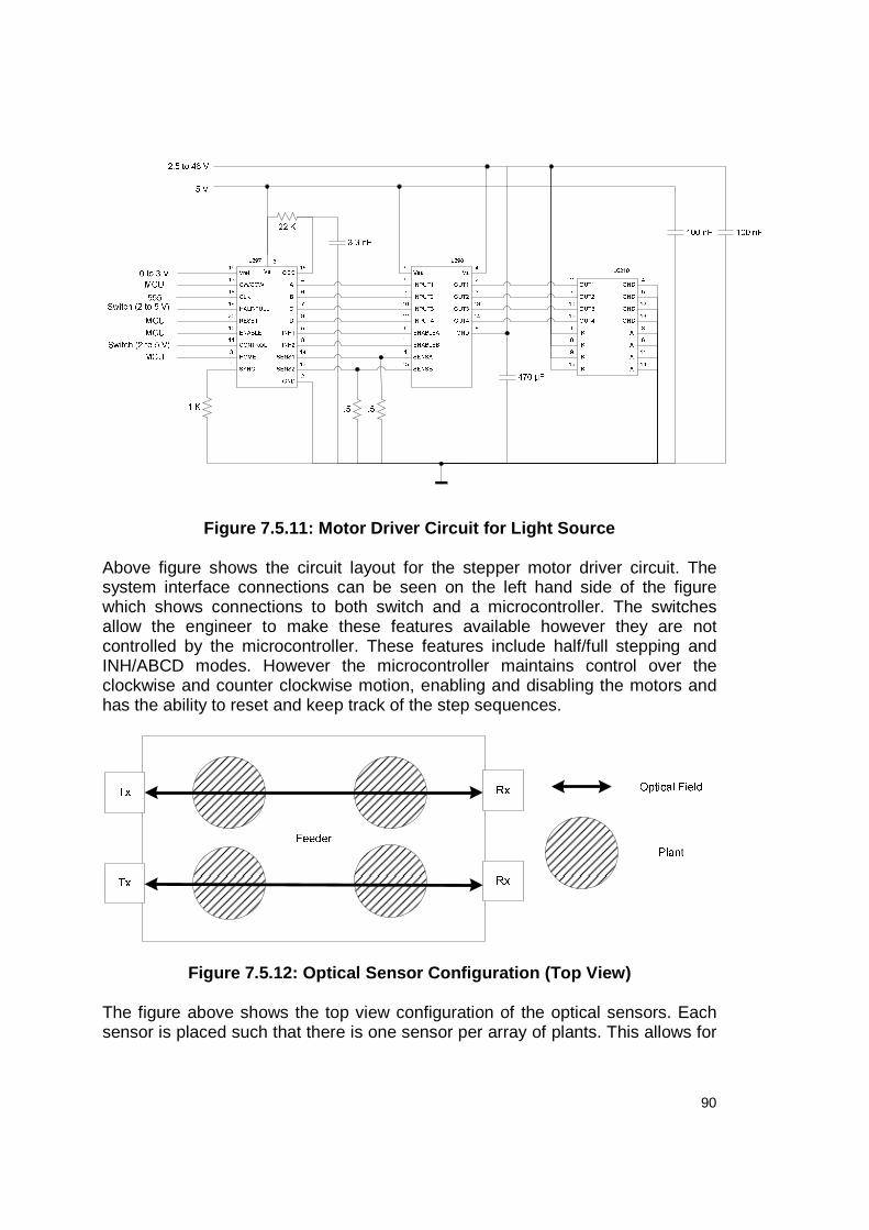
90

Figure 7.5.11: Motor Driver Circuit for Light Sourc e

Above figure shows the circuit layout for the stepper motor driver circuit. The system interface connections can be seen on the left hand side of the figure which shows connections to both switch and a microcontroller. The switches allow the engineer to make these features available however they are not controlled by the microcontroller. These features include half/full stepping and INH/ABCD modes. However the microcontroller maintains control over the clockwise and counter clockwise motion, enabling and disabling the motors and has the ability to reset and keep track of the step sequences.

Figure 7.5.12: Optical Sensor Configuration (Top Vi ew)

The figure above shows the top view configuration of the optical sensors. Each sensor is placed such that there is one sensor per array of plants. This allows for

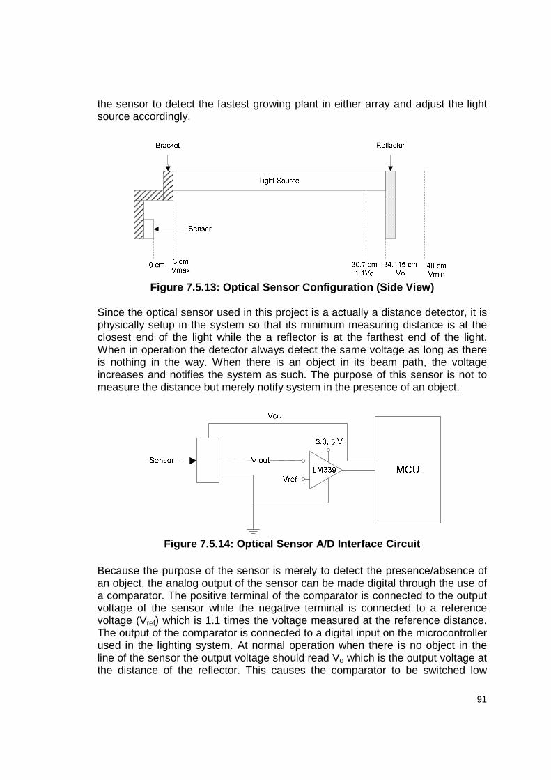
91

the sensor to detect the fastest growing plant in either array and adjust the light source accordingly.

Figure 7.5.13: Optical Sensor Configuration (Side V iew)

Since the optical sensor used in this project is a actually a distance detector, it is physically setup in the system so that its minimum measuring distance is at the closest end of the light while the a reflector is at the farthest end of the light. When in operation the detector always detect the same voltage as long as there is nothing in the way. When there is an object in its beam path, the voltage increases and notifies the system as such. The purpose of this sensor is not to measure the distance but merely notify system in the presence of an object.

Figure 7.5.14: Optical Sensor A/D Interface Circuit

Because the purpose of the sensor is merely to detect the presence/absence of an object, the analog output of the sensor can be made digital through the use of a comparator. The positive terminal of the comparator is connected to the output voltage of the sensor while the negative terminal is connected to a reference voltage (Vref) which is 1.1 times the voltage measured at the reference distance. The output of the comparator is connected to a digital input on the microcontroller used in the lighting system. At normal operation when there is no object in the line of the sensor the output voltage should read Vo which is the output voltage at the distance of the reflector. This causes the comparator to be switched low

92

which provides a grounded output of zero. When an object is enters the line of the sensor the voltage increases. If that voltage is greater than Vref, the comparator switches high and signals the microcontroller to move the light up. The purpose of the 1.1 factor is to allow for an error in the voltage so that fluctuations do not falsely trigger the microcontroller to move the light.

Figure 7.5.15: GE Contact Sensor Digital Interface

The GE configuration utilizes a comparator circuit where the output of the sensor is connected to the negative terminal and a reference voltage is connected to the input of the positive terminal. The reference voltage can take on the minimum voltage required by the comparator as long as it is greater than zero. When the magnet is out of range of the sensor, the circuit is closed and the output voltage forces the output of the comparator to ground. When the magnet makes contact with the sensor, the circuit opens which causes the output of the comparator to go high. In the case of the digital sensor a non-inverting amplifier is connected between the sensor and the microcontroller which provides a gain of 10. This makes the maximum input to the microcontroller 5 V. Also, there exists a pull-up resistor between the supply voltage and the output voltage of the sensor which forces the output to go high when the magnet is in contact with the sensor.

Figure 7.5.16: Cherry Contact Sensor Digital Interf ace

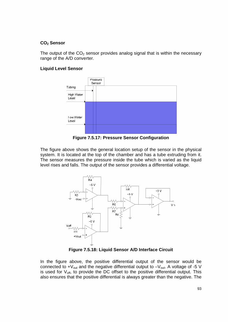
93

CO2 Sensor The output of the CO2 sensor provides analog signal that is within the necessary range of the A/D converter. Liquid Level Sensor

Figure 7.5.17: Pressure Sensor Configuration

The figure above shows the general location setup of the sensor in the physical system. It is located at the top of the chamber and has a tube extruding from it. The sensor measures the pressure inside the tube which is varied as the liquid level rises and falls. The output of the sensor provides a differential voltage.

Figure 7.5.18: Liquid Sensor A/D Interface Circuit

In the figure above, the positive differential output of the sensor would be connected to +Vout and the negative differential output to –Vout. A voltage of -5 V is used for Voff, to provide the DC offset to the positive differential output. This also ensures that the positive differential is always greater than the negative. The

94

outputs of those amplifiers are then connected to a difference amplifier which has the gain of 500. Before sending the input into the microcontroller, a buffer is used to provide protection for the microcontroller against fluctuations. Given the minimum differential output of 0 mV and a maximum differential output of 5 mV, the resulting output of the connecting circuit is 2.5 V to 5 V.

Temperature Sensor

Figure 7.5.19: Temperature Sensor A/D Interface Cir cuit

Chemical Regulation

Figure 7.5.20: Peristaltic Pump

The above figure shows the basic setup of a peristaltic pump which is the pump type that is used to disperse the chemicals into the plant feed. It operates by turning in a circular fashion where compressed tubing contains small amounts of liquid in the gaps between the pegs. The main components consist of a disk with evenly spaced pegs extruding from it. Starting from one side of the support, silicon tubing is routed up through a hole and stretched around the pegs such that the pegs act as barriers by compressing the tube and allow a small space for liquid to be stored. As the disk is rotated, the pocket of liquid remains constant and exits out the other side. As the pump continues this process, liquid is continuously filled into these discrete pockets by creating its own pressure and drawing liquid from a reservoir. The idea control for this type of setup would be a stepper motor which allows for precise turns of the disk.

95

Figure 7.5.21: Pump Motor Driver Circuit Configurat ion

It was decided that at no point and time are any of the motors running simultaneously, therefore in order to maximize the outputs of the microcontroller all three pump motors is powered using a signal from a de-multiplexer which is controlled by the microcontroller. In this configuration the motors would actually be on the same multiplexer as other components which would also not need to be controlled simultaneously. Because stepper motors is used for the rotation of the pump, a stepper driver circuit is needed just as it had been required with the lighting system. In fact, a similar circuit is employed, however the control of the motor is simplified based on the characteristics of its use. Meaning, it only needs to travel in one direction, it only operates in half stepping mode, the enable ability is controlled by a de-multiplexer and it does not have the additional HOME and RESET control features. One additional feature that is implemented is the ability of the driver circuits to slave off of one main driver circuit which has the input of the RC oscillator. The configuration of the elements can be seen in the figure below.

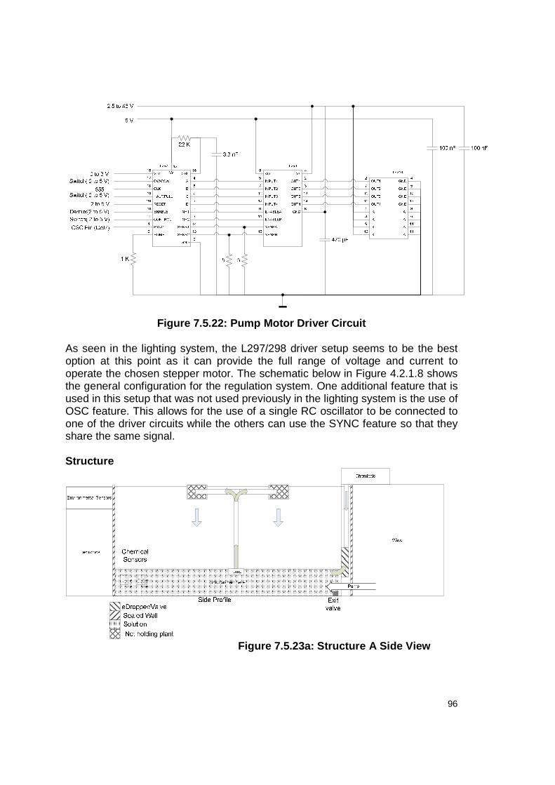
96

Figure 7.5.22: Pump Motor Driver Circuit

As seen in the lighting system, the L297/298 driver setup seems to be the best option at this point as it can provide the full range of voltage and current to operate the chosen stepper motor. The schematic below in Figure 4.2.1.8 shows the general configuration for the regulation system. One additional feature that is used in this setup that was not used previously in the lighting system is the use of OSC feature. This allows for the use of a single RC oscillator to be connected to one of the driver circuits while the others can use the SYNC feature so that they share the same signal. Structure

Figure 7.5.23a: Structure A Side View

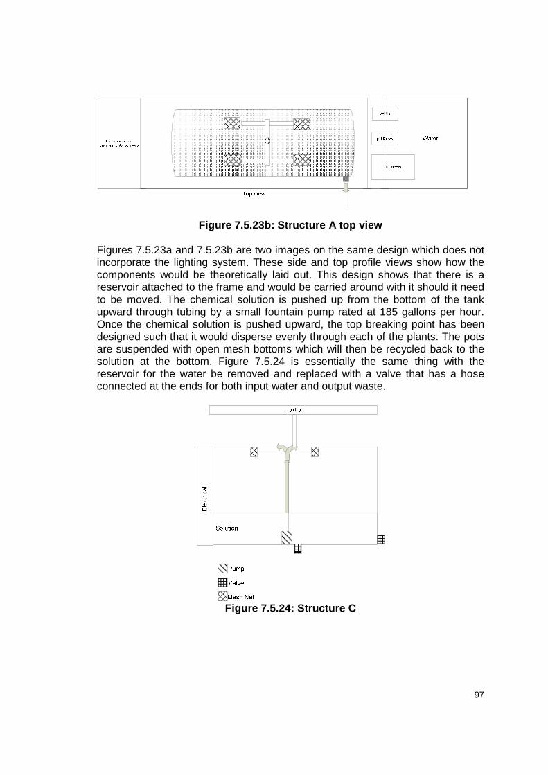
97

Figure 7.5.23b: Structure A top view

Figures 7.5.23a and 7.5.23b are two images on the same design which does not incorporate the lighting system. These side and top profile views show how the components would be theoretically laid out. This design shows that there is a reservoir attached to the frame and would be carried around with it should it need to be moved. The chemical solution is pushed up from the bottom of the tank upward through tubing by a small fountain pump rated at 185 gallons per hour. Once the chemical solution is pushed upward, the top breaking point has been designed such that it would disperse evenly through each of the plants. The pots are suspended with open mesh bottoms which will then be recycled back to the solution at the bottom. Figure 7.5.24 is essentially the same thing with the reservoir for the water be removed and replaced with a valve that has a hose connected at the ends for both input water and output waste.

Figure 7.5.24: Structure C

98

pH Probe

Figure 7.5.25 pH probe

Permission requested from VirtualVillage.com There are plenty of replacement probes on the market today for universal setups. The idea behind this method is that you can take a probe that is made for many products and base your circuit around these outputs. While there were large varieties out there, the one that seemed to have the easiest and widest selection of product was a BNC based connection. Nutrient Sensor TDS sensing has been selected as just a replacement probe itself. Looking at possible products that are within reasonable price range, the company that we are getting out pH meter from seems to have a selection of probes. These probes are sometimes a little bit more difficult to tap into as opposed to the pervious pH meters were. In an email sent to Hanna Instruments it first informs the company that, “I sent an email a couple days ago requesting permission to use an image off of this website for a research paper our group of electrical engineers are conducting at the University of Central Florida.” The letter goes on to ask “if this company carried a TDS probe that has a BNC connector.” With the Din cables that I have seen that other companies as well as this one offer could possibly be a point where there is a halt to the sensing of pH because of the lack of any reference or data sheet. So far there are two different products that are under review by the group. Both are probes that are added to existing systems. This already is a more difficult task as before because the connections are much different. The concept does remain the same and for that there is a little hope that the same success can be replicated. The difference here is that it is now a din cable as opposed to the BNC connector that was used prior which makes things interesting for the microprocessor.

99

Chapter 8: Testing

8.1 Facilities and Equipment The engineers will utilize the test equipment in the senior design lab and test equipment available at the team member’s homes. This includes oscilloscopes, function generators, power supplies, multi-meters, bread boards and other engineering equipment available. While the system is in development it will most likely be stored at the team member’s homes. If work needs to be done in the senior design lab, the team members will transport the system as needed.

8.2 Testing Procedures The microcontrollers and web interface is utilized as part of all testing procedures as needed. For instance, the web interface is tested when testing the pumps and valves and the microcontroller is tested throughout each of the systems in the following sections.

8.2.1 Sensors pH Sensor

The testing of this sensor can be accomplished in one of two ways. The first utilizes a chemical testing kit that can be purchased at low cost. The second method would be through the use of a digital meter which would be available for purchase at a much higher cost. This method would provide a much more accurate means of testing given that the instrument being used has been correctly calibrated. It may be possible to borrow a meter such as this through various campus organizations such as the Arboretum, Chemical/Biology Department or possibly through the UCF Storm Water Academy. This sensor is compared to the sensor in the system and tested against multiple solutions to see if they give the same pH value.

Nutrient Sensor

To test the nutrient sensor a control solution is needed. The sensor will first be tested with water which would give a baseline reading (most likely of 0ppm). Then a fixed amount of nutrients is added where the engineer testing the solution will know the ppm of the nutrients to water mixture. Then sensor will then be placed in this solution and the reading is checked. The next step is to check if the sensor senses change. Therefore, the same amount of nutrients is added to the solution again and the ppm should double on the reading from the sensor.

Solution Level

The testing of this sensor will most likely utilize the simplest means through the use of a ruler or tape measure. Using these basic tools accuracy is available

100

down to the millimeter which would be the ideal accuracy of the sensor. Such equipment can be purchased or acquired at little to no cost.

Humidity and Temperature

This sensor can easily be tested using a relatively inexpensive digital hygrometer. Typical hygrometers of this type are available with a temperature accuracy of less than 1o C and a humidity accuracy of 1%, both of which meet the necessary minimum for this project.

CO2 Sensor

Unfortunately this sensor is very difficult to test because standard fixed CO2 measurements are not known. Since the sensor is said to be pre-calibrated it is tested against the standard measurement for atmospheric CO2 which is taken from resources online at the time of testing. The sensor will then be placed in a closed system and a baseline reading is taken. A CO2 canister is released into the system and another reading is taken. The difference of the two reading is taken and if the difference is equal to the amount of CO2 in the canister then the sensor is deemed as tested and working.

8.2.2 Lighting The Lighting system is tested by manipulation of the system and the environment. The day and night cycles is tested by setting the cycles to short intervals and timing them to make sure the lights turn on and off as specified by the user. The distance of the lighting system is tested by placing the system at its lowest possible setting and blocking the optical sensor. The system should respond by raising the lights by a fixed value which will then be measured by the engineers to check if the system is responding correctly. The light will then be moved right below the highest possible point and the optical sensor is blocked once again. The system is deemed as functioning correctly if stops upon contact with the highest possible point.

8.2.3 Pumps and Valves Valves

The valves is tested when implemented into the system. The valves is checked if they open when the microcontroller tells it to open and if they close when the microcontroller tells it to close. The seal on the valve will also be checked for leaks by placing it into the system and see if they can handle the amount of water pressure placed on them while being in the system. The valves will also be checked to see if they can function through normal operation of the system, such as draining and filling the system to the exact specifications defined by the user through the interface.

101

Pumps

The pumps is tested once the sensors are deemed to be working. This will ensure accurate function of the pumps in the system. The pumps is told to raise the pH or lower the pH to a certain value and then the sensor measures the value. If the measured value is equal to that of the defined value then the pH pump is working correctly. The nutrient sensor is tested in the same manner as the pH motor, however it uses nutrients instead of pH to check for only raising the nutrient concentration.

8.2.4 Power System The power system needed to be tested because of the distribution of power and the use of DC and AC voltages. A multi-meter and oscilloscope is used to test the power being distributed to each part of the system, including the microcontrollers, sensors, pumps and relays. The power system is tested by using the test equipment to measure the power at each point with the load of the different apparatuses attached to it. By testing the power systems in this manner it will safely check to make sure the power is being distributed accordingly and therefore protects the user and the equipment.

Summary and Conclusions The main goal of this project is to build an automated system that can monitor and regulate environmental conditions for growing plants. This paper serves as research for feasibly building this system and organizing ideas. With strong enough research and foresight in designing the system this paper should prove to give the engineers a clear direction on how to build the entire system.

The microcontroller that we plan to use for our project is the ATmega168 microcontroller which is excellent for its easy programming language and its computing power. It is used in conjunction with the Lantronix MatchPort b/g Pro, which provides a wireless interface that can be used to connect to the system both locally and externally from the network. In addition, the system provides a data logging capability and database which is stored on a Secure Digital Card, and accessed using the web based user interface. The microcontroller reads in measurements from different sensors and regulates using different devices to control the environmental growth factors for the plants. These sensors used include temperature, CO2, Liquid Level, Humidity, Nutrient and a pH sensor. The system is able to adjust environmental conditions such as pH, nutrients and liquid level which is accomplished through the use of homemade peristaltic type pumps. We chose to use a separate microcontroller for the lighting system because it would be easier to control the lighting system if it only passed user-defined values. The lighting system is very intricate in the fact that it maintains a fixed height above the plant automatically as the plant grows and also regulates day and night cycles. Additionally, the power system distributes the necessary power to each of the valves, regulators, microcontrollers, and sensors.