Automated Operator Link Assignment Scheduling for NASA’s Deep Space Network Daniel Tran* and Mark D. Johnston*

*Jet Propulsion Laboratory, California Institute of Technology 4800 Oak Grove Drive, Pasadena CA USA 91109

{daniel.tran, mark.d.johnston} @jpl.nasa.gov

Abstract NASA’s Deep Space Network (DSN) provides communica-

tion and other services for planetary exploration for both NASA and international users. The DSN operates antennas at three complexes: Goldstone, California, USA; Madrid, Spain; and Canberra, Australia, with the longitudinal distribution of the com- plexes enabling full sky coverage and generally providing some overlap in spacecraft visibility. Beginning in 2018, the DSN will be transitioning to a remote operations paradigm where local day- shift operators at each complex will be preparing and staffing the links (or contacts) for all antennas in the DSN. In addition, the number of simultaneous links an operator will be required to sup- port will increase from two (today) to three. In this paper, we describe the impact of these two changes on scheduling — in- cluding modeling link complexity and the generation of auto- mated operator link assignments. Minimizing the combined com- plexity of the multiple links assigned to a single operator is emerging as a key tool in achieving the DSN’s overall automation objectives. We describe the results to date of a prototype link assignment algorithm and corresponding user interface, and plans for future work that include user trials and sensitivity studies of various complexity metrics.

1. Introduction The NASA Deep Space Network (DSN) consists of three large complexes of antennas, spaced roughly evenly in longitude around the world at Goldstone, California; Ma- drid, Spain; and Canberra, Australia. Each complex con- tains one 70 meter antenna along with a number of 34 me- ter and smaller antennas, as well as the electronics and networking infrastructure to command and control the an- tennas and to communicate with various mission control centers. Figure 1 summarizes the DSN Deep Space Com- munications Complexes (DSCC) including their locations and antennas; for more extensive background on the DSN, refer to [1,2].

All NASA planetary and deep space missions, as well as many international missions, communicate to Earth through the DSN. In some cases, missions closer to Earth also use the DSN, some routinely, others on an occasional basis. The capabilities of the DSN make it a highly capable scientific facility in its own right, so it is used for radio astronomy (including very long baseline interferometry) as well as radio science investigations. At present, there are 37 regular distinct users of DSN, who together schedule

Copyright © 2015, California Institute of Technology. Government spon- sorship acknowledged.

about 500 activities per week on 13 antennas. Over the next few decades, utilization of the DSN is expected to grow significantly, with more missions operating, higher data rates and link complexities, and the possibility of manned mission support. In addition, the total number of antennas will grow to 18, while at the same time there is pressure to reduce ongoing costs yet maintain an around- the-clock operational capability.

Presently, each of the DSN complexes is staffed 24x7 with local personnel who manage the antenna/spacecraft links. The individuals directly responsible for this are des- ignated Link Control Operators, or LCOs. In general, each LCO manages up to two links at a time. Future plans for increased automation are presently in progress, which will have two fundamental shifts in operations: • “Follow the Sun” Operations (FtSO) — at each com-

plex during their local day shift, each complex will operate not only their local assets, but also all the assets of the other two complexes as well, via remote control.

• Three Links per Operator (3LPO) — the number of links a LCO will manage will increase from two (to- day) to three.

These changes represent a major paradigm shift and will require numerous software changes to improve DSN auto- mation, as well as WAN upgrades to increase bandwidth and reliability of complex-to-complex communications. The benefit will be a significant savings in operations costs while continuing to provide high-quality support to DSN users.

In this paper we first give a general overview of the DSN scheduling process (Sect 2) followed by a brief de- scription of the changes to be introduced by the Follow- the-Sun paradigm shift (Sect 3). We then describe our ap- proach to helping the operations staff manage the complex- ity of remote operations as well as the increasing number of simultaneous links per operator (Sect 4). We describe some algorithmic experiments we have undertaken to ex- plore different approaches to scheduling while smoothing out the operator workload (Sect 5). Finally, we conclude with a discussion of plans for next steps (Sect 6).

2. DSN Scheduling: Process and Software The DSN scheduling process consists of three main phases, which do not have sharply defined boundaries. In this sec- tion we briefly describe these phases as they exist today.

113

Fig. 1 Overview of DSN complexes and their complement of antennas.

• Long-Range Planning and Forecasting. Long-range

planning is based on user-provided high-level require- ments. Long-range planning has several major pur- poses:

− studies and analyses: periods of particular interest or concern are examined to determine where there is likely contention among missions, or when con- struction or deployment of new DSN assets are under investigation

− downtime analysis: identifying periods of time when necessary antenna or other maintenance can be scheduled, attempting to minimize the impact on missions

− future mission analysis: in their proposal phases, missions can request analysis of their expected DSN coverage as part of assessing new mission feasibility and cost

The time range for long-range planning is generally six months or more into the future, sometimes as much as several years.

• Mid-Range Scheduling. The mid-range scheduling phase is when detailed user requirements are specified, integrated, negotiated, and all tracking activities final- ized in the schedule. Starting at roughly 4-5 months

before execution, users specify their detailed schedul- ing requirements on a rolling weekly basis. These re- quirements include:

− tracking time and services required − constraining time intervals and relationships − visibility constraints − flexibilities

More details on these various types of scheduling re- quirements are provided elsewhere[3,4]. Once the deadline passes and all requirements are in, the full set is integrated into an initial schedule in which conflicts are automatically reduced by taking advantage of what- ever flexibilities have been specified. There follows an optimization step where an experienced DSN scheduler interactively edits the schedule and further reduces conflicts by taking advantage of unspecified flexibilities and making further adjustments. It is then released to the scheduling user community who negotiate to elimi- nate remaining conflicts and to further optimize cover- age for their missions. This is considered the “negoti- ated schedule” that missions use to plan their integrated ground and spacecraft activities, including the devel- opment of onboard command loads based in part on the DSN schedule. Following this point, changes to the schedule may still occur, but new conflicts may not be

Under construction

9/2014 9/2016

DSSG24 DSSG25 DSSG26 34m (BWGG1) (BWGG2) (BWGG3)

DSSG23 (BWGG4)

DSSG54 DSSG55 34m (BWGG1) (BWGG2)

DSSG56 (BWGG3)

DSSG34 DSSG35 34m (BWGG1) (BWGG2)

DSSG36 (BWGG3)

DSSG14 70m

Signal Processing Center SPCG10 DSSG63

70m

Signal Processing Center SPCG60 DSSG43

70m

Signal Processing Center SPCG40

DSSG15 34m High Efficiency (HEF)

DSSG13 34m BWG & HP Test Facility

DSSG65 34m High Efficiency (HEF)

DSSG53 (BWGG4)

DSSG45 34m High Efficiency (HEF)

DSSG33 (BWGG4)

Goldstone Barstow, CA, USA

Madrid, Spain

Canberra, Australia

MIL%71 DSN’s KSC

Network Opera#ons Control Center at JPL, Pasadena , CA

114

introduced. There is a continuing low level of no- impact changes and negotiated changes that occur all the way down to execution.

• Near Real-time Scheduling. The near real-time phase of DSN scheduling starts roughly three weeks from exe- cution and includes the period through execution of all the scheduled activities. Late changes may occur for various reasons (sometimes impacting the mid-range phase as well):

− users may have additional information or late changes to requirements for a variety of reasons

− DSN assets (antennas, equipment) may experience unexpected downtimes that require adjustments to the schedule to accommodate

− spacecraft emergencies may occur that require ex- tra tracking or changes to existing scheduled ac- tivities

For many missions that are sequenced well in advance, late changes cannot be readily accommodated.

The DSN scheduling software is called Service Schedul- ing Software, or S3[3,4]. It was initially applied to the mid- range phase of the process, but is being extended to cover all three phases. S3 provides a Javascript-based HTML5 web application and integrated database[10] through which users can directly enter their own scheduling requirements and verify their correctness before the submission deadline. The database in which requirements are stored is logically divided into “master” and “workspace” areas. There is a single master schedule representing mission-approved re- quirements and DSN activities (tracks). Each user can cre- ate an arbitrary number of workspace schedules, initially either empty or based on the contents of the master, within which they can conduct studies and 'what if' investigations, or keep a baseline for comparison with the master. These workspaces are by default private to the individual user, but can be shared as readable or read-write to any number of other users. Shared workspaces can be viewed and up- dated in realtime: while there can only be one writer at a time, any number of other users can view a workspace and see it automatically update as changes are made. These aspects of the web application architecture and database design support the collaborative and shared development nature of the DSN schedule.

In addition, S3 offers specialized features to facilitate collaboration, including an integrated wiki for annotated discussion of negotiation proposals, integrated chat, notifi- cations of various events, and a propose/concur/reject/ counter workflow manager to support change proposals. Details on the design and use of the S3 collaboration fea- tures[5] and the scheduling engine[6,7] are provided else- where.

3. Scheduling in the Follow-the-Sun Era There are three major changes to the scheduling process that are expected to come with FtSO:

• Scheduling from the complexes: the scheduling system will be made available for use at the complexes di- rectly, to enter and manage activities such as mainte- nance and engineering. In addition, operators will be able to make other schedule changes to help manage their workload, such as starting setup for an activity earlier than usual, or extending teardown later. Such changes do not impact mission users of the DSN, but give the operations staff more flexibility.

• Automated rescheduling support: with the integration of S3 to support realtime, and access to realtime asset status as well as detailed requirements and flexibilities of individual activities, S3 can be used to generate al- ternative rescheduling options when late breaking schedule changes occur. These can be due to any of the reasons noted above that can affect the real-time sched- ule. In today’s operations, such changes require a great deal of back and forth between the users and operations staff to come up with minimal impact schedule changes. Use of automated scheduling s/w to provide suggestions and options is expected to help facilitate this exchange.

• Link complexity scheduling: not all activities are equally demanding, and when LCO are managing mul- tiple activities at once it is easy to see that inadvertent overloading of the operations staff is a potential risk. As a result, we are investigating how to model the complexity of individual activities, and then to avoid overloading individual LCOs with too much work at one time. There are two major parts to this effort:

− a) during schedule generation (weeks to months ahead of execution): to predict the occurrence of ‘spikes’ in loading and provide feedback to users so they can make adjustments early in the process before the schedule is firm; in addition, higher pe- riods of link complexity could serve as early warn- ing that additional or overtime staffing may be required to cover a particular time frame or critical event

− b) during shift planning (hours to days ahead of execution): to determine a good assignment of work to operators that does not exceed threshold values for number of links or overall link complex- ity, and which, as much as possible, evenly distrib- utes the work across the available operations staff.

In the remainder of this paper we concentrate on link complexity scheduling during shift planning as a new area of development with significant uncertainty.

4. The Role of Link Complexity The concept of link complexity is intended to capture a measure of the workload of the Link Control Operator (LCO) while managing the three stages of a typical DSN- to-spacecraft link: setup, in-track, and teardown. This con- cept, to date, is not quantitative: there is no direct measure of how much concentration or mental energy is expended

115

on a particular type of link. Several internal studies of link complexity have been conducted, which have investigated indicators of complexity based on measured quantities. One of the most promising indicator is termed “Operator Directive” (OD) count, which reflects the LCO issuing commands or responding to pop-up dialogs. High OD rates would be expected to correspond to high levels of attention and thus higher complexity.

At a high level there are three phases to a link: • setup: this ranges in duration from about 30 minutes to

over an hour, depending on what services are required. It includes moving the antenna from its stowed position to the proper pointing, and configuring the needed equipment (receivers, transmitters, telemetry proces- sors, array combiners, etc.)

• in-track: the actual spacecraft activity, consisting of one or more services such as downlink of telemetry, uplink of commands or other data, acquisition of navigation data, etc. A typical in-track phase runs from about an hour in duration up to about 12 hours.

• teardown: at the conclusion of the in-track phase, the equipment is removed from the link and the antenna is returned to stow. This phase is nearly always 15 min- utes in duration

The start of each one of these three phases is observed to require additional operator attention, which normally re- duces over time as the connection is configured, the track starts, or the connection is dissolved. Depending on exactly what is planned to occur during a track, the LCO may have to re-engage for some time to verify and interact with the system: for example, if there is a planned data rate change or other spacecraft reconfiguration, the LCO may need to monitor carefully for a time to ensure that all is well, and intervene if necessary.

Certain types of activities that fall into the category of a single ‘link’ are observed to require more than typical at- tention. Among these are multi-spacecraft and multi- antenna activities such as the following: • Multiple spacecraft per antenna (MSPA): this case in-

cludes a frequently used capability to downlink data from two spacecraft simultaneously, and uplink to one, where the specific spacecraft can change. This provides a large efficiency boost, primary for missions at Mars (where there are currently 7 spacecraft) but occasion- ally for other missions. As missions enter and leave the connection, the operator is required to pay extra atten- tion that all is working as expected.

• Multi-antenna activities: there are two common cases for this situation — (1) Doppler measurements for navigation (DDOR1), and (2) arrays of between two and four antennas that provide a larger equivalent aper- ture for higher sensitivity or data rates. Because all the antennas involved are interdependent and must be

monitored, these cases have higher intrinsic complexity than single spacecraft, single antennas activities.

The other major factor that needs to be taken into ac- count in modeling complexity is that of external events, most notably shift change and handover. In the FtSO para- digm, each complex hands off ongoing activities to another complex when their day shift ends. During handoff, each LCO will be informing their successor of the state of the link and of any special considerations. During this time, the source and destination LCOs are more than normally occupied with their work, and so their capacity to take on new high-complexity activities is reduced.

It is not known how link complexity combines in multi- link situations, for example for operators who are manag- ing two links at once, or up to three in the future. However, it is reasonable to assume an additive combination function as a working hypothesis, and we make that assumption in the following.

At the current time, constraints are in place that proxy link complexity. For example, at the Goldstone complex, no more than two links may start at the same time, and additional links have to be separated by at least 15 minutes. Such a rule was put in place when Goldstone only operated its own 5 antennas; with FtSO it will be operating 13 or more and so it is evident that the rules will have to be re- considered.

5. Prototype and Experiments As part of assessing the impact of higher link complex-

ity in FtSO, and mitigating the risk of remote operations and 3LPO, we have developed a prototype and testbed for exploring link complexity models and scheduling algo- rithms. Link Assignment Algorithm

Our scheduling problem consists of a model of the op- erators and a schedule of links as inputs. The operator model contains of two timelines: • Link count – an integer resource measuring the number

of links assigned to the operator. • Complexity value – a floating point resource measuring

the total complexity of the links assigned to the opera- tor.

Each of the timelines has an associated limit, such that exceeding the limit for any duration is considered a con- flict.

For this prototype, complexity values for concurrent scheduled links on one operator are summed, though we expect this to be revised in the future based on user feed- back. When computing the complexity of a link, the com- plexity function is applied across three distinct sections of a link — setup, in-track, and teardown.

1 Delta Differential One-way Ranging

116

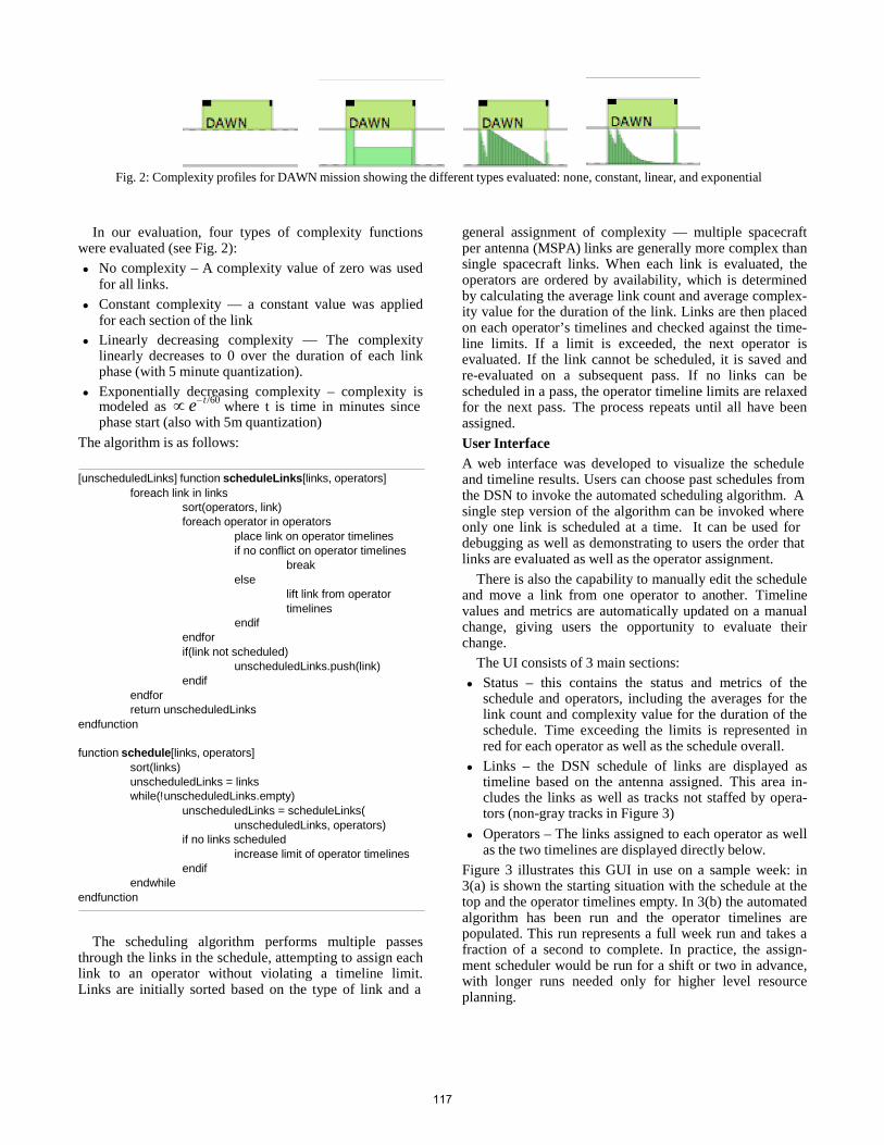
Fig. 2: Complexity profiles for DAWN mission showing the different types evaluated: none, constant, linear, and exponential

In our evaluation, four types of complexity functions were evaluated (see Fig. 2): • No complexity – A complexity value of zero was used

for all links. • Constant complexity — a constant value was applied

for each section of the link • Linearly decreasing complexity — The complexity

linearly decreases to 0 over the duration of each link phase (with 5 minute quantization).

• Exponentially decreasing complexity – complexity is modeled as ∝ e− t /60 where t is time in minutes since phase start (also with 5m quantization)

The algorithm is as follows:

[unscheduledLinks] function scheduleLinks[links, operators] foreach link in links

sort(operators, link) foreach operator in operators

place link on operator timelines if no conflict on operator timelines

break else

lift link from operator timelines

endif endfor if(link not scheduled)

unscheduledLinks.push(link) endif

endfor return unscheduledLinks

endfunction

function schedule[links, operators] sort(links) unscheduledLinks = links while(!unscheduledLinks.empty)

unscheduledLinks = scheduleLinks( unscheduledLinks, operators)

if no links scheduled increase limit of operator timelines

endif endwhile

endfunction

The scheduling algorithm performs multiple passes through the links in the schedule, attempting to assign each link to an operator without violating a timeline limit. Links are initially sorted based on the type of link and a

general assignment of complexity — multiple spacecraft per antenna (MSPA) links are generally more complex than single spacecraft links. When each link is evaluated, the operators are ordered by availability, which is determined by calculating the average link count and average complex- ity value for the duration of the link. Links are then placed on each operator’s timelines and checked against the time- line limits. If a limit is exceeded, the next operator is evaluated. If the link cannot be scheduled, it is saved and re-evaluated on a subsequent pass. If no links can be scheduled in a pass, the operator timeline limits are relaxed for the next pass. The process repeats until all have been assigned. User Interface A web interface was developed to visualize the schedule and timeline results. Users can choose past schedules from the DSN to invoke the automated scheduling algorithm. A single step version of the algorithm can be invoked where only one link is scheduled at a time. It can be used for debugging as well as demonstrating to users the order that links are evaluated as well as the operator assignment.

There is also the capability to manually edit the schedule and move a link from one operator to another. Timeline values and metrics are automatically updated on a manual change, giving users the opportunity to evaluate their change.

The UI consists of 3 main sections: • Status – this contains the status and metrics of the

schedule and operators, including the averages for the link count and complexity value for the duration of the schedule. Time exceeding the limits is represented in red for each operator as well as the schedule overall.

• Links – the DSN schedule of links are displayed as timeline based on the antenna assigned. This area in- cludes the links as well as tracks not staffed by opera- tors (non-gray tracks in Figure 3)

• Operators – The links assigned to each operator as well as the two timelines are displayed directly below.

Figure 3 illustrates this GUI in use on a sample week: in 3(a) is shown the starting situation with the schedule at the top and the operator timelines empty. In 3(b) the automated algorithm has been run and the operator timelines are populated. This run represents a full week run and takes a fraction of a second to complete. In practice, the assign- ment scheduler would be run for a shift or two in advance, with longer runs needed only for higher level resource planning.

117

(a)

(b)

Fig. 3: Screenshots of prototype link complexity assignment GUI. (a) the original schedule with no assignments; (b) after running the complexity-based scheduling algorithm: the operator timelines at the bottom represent the workloads for a hypothetical four operators, scheduling three links apiece.

The prototype has several additional controls in use for experiments with users and for algorithm assessment: • profile selection — none, constant, linear, exponential • selection criteria — consider both number of link and

complexity limits, consider complexity only, consider link count only.

• enable handover avoidance — when checked, this re- duces the complexity limit at times of each shift han- dover, to reflect lower limits on complexity during these times

• enable remote ops — when checked, all DSN antennas are scheduled as a single group, simulating the opera- tion of the entire network by one complex that is re-

118

motely controlling the whole network; otherwise, each complex is scheduled separately (mirroring today’s operation)

• render links as tracks — when checked, collapse multi- ple activities into a single bar per link

6. Results and Conclusions So far we have demonstrated this prototype GUI to the Canberra DSCC operations staff (Fig. 4) with very positive feedback. Several clear challenges remain: • determining an appropriate scale for the complexity

measure will require a combination of LCO input and analysis of OD data, correlated with track type and at- tributes. The LCO have expressed interest in participat- ing in this determination, and we are looking into vari- ous methods for eliciting relative preferences for differ- ent complexity profiles.

• the required degree of modeling of individual operator availability and capability remains an open question. For example, trainees may be limited in the number of links they are allowed to take on at once, or their com- plexity. There may be labor rules, possibly differing from one complex to another, that have to be consid- ered.

• the impact of shift changes and handoff is not yet well understood. Current plans are for one LCO at the source site to handoff to one LCO at the destination site, but this remains to be evaluated and may change.

• how much to push the link complexity assessment up- stream remains an open question — for example, to treat complexity spikes as ‘conflicts’ that must be re- solved, like any type of conflict such as overbooking antennas or equipment.

Despite these challenges, the link complexity scheduler is one of the pro-active steps being taken to manage the in- crease in complexity expected in the remote operations era, and is expected to be a flexible and effective way to help smooth the evolution to a new DSN operations paradigm.

The research described in this paper was carried out at the Jet Propulsion Laboratory, California Institute of Technol- ogy, under a contract with the National Aeronautics and Space Administration. We gratefully acknowledge the sup- port of the DSN scheduling community over the course of this work, and particularly to Erik Barkley and Sil Zende- jas for study results of potential link complexity metrics.

Bibliography

[1] J.B. Berner, J. Statman, Increasing the cost-efficiency of the DSN, in: Heidelberg, Germany, 2008.

[2] W.A. Imbriale, Large Antennas of the Deep Space Network, Wiley, 2003.

[3] M.D. Johnston, D. Tran, B. Arroyo, S. Sorensen, P. Tay, J. Carruth, et al., Automating Mid- and Long-Range Schedul- ing for NASA's Deep Space Network, in: SpaceOps 2012, Stockholm, Sweden, 2012.

[4] M.D. Johnston, D. Tran, Automated Scheduling for NASA's Deep Space Network, in: IWPSS 2008, Darmstadt, Ger- many, 2011.

[5] J. Carruth, M.D. Johnston, A. Coffman, M. Wallace, B. Ar- royo, S. Malhotra, A Collaborative Scheduling Environment for NASA's Deep Space Network, in: SpaceOps 2010, AIAA, Huntsville, AL, 2010.

[6] M.D. Johnston, D. Tran, B. Arroyo, C. Page, Request-Driven Scheduling for NASA’s Deep Space Network, in: Pasadena, CA, 2009.

[7] S. Chien, M.D. Johnston, J. Frank, M. Giuliano, A. Kave- laars, C. Lenzen, et al., A generalized timeline representa- tion, services, and interface for automating space mission operations, in: Proceedings of SpaceOps 2012, Stockholm, 2012.

Figure 4. The prototype link complexity GUI running at the Canberra Deep Space Communications Complex dur- ing a demonstration.

119