automated multiobjective optimisation in axial compressor

1 Copyright © #### by ASME

Proceedings of GT2006 ASME Turbo Expo 2006: Power for Land Sea and Air

8-11 May 2006, Barcelona, Spain

GT2006-90420

AUTOMATED MULTIOBJECTIVE OPTIMISATION IN AXIAL COMPRESSOR BLADE DESIGN

Christian Voß, Marcel Aulich, Burak Kaplan and Eberhard Nicke Institute of Propulsion Technology

German Aerospace Centre, Cologne ABSTRACT

This paper presents an automated multiobjective design methodology for the aerodynamic optimisation of turbomachinery blades. In this approach several operating-points of the compressor are considered and the flow-characteristics of the different flow-solutions are combined to one or more objective functions.

The optimisation strategy is based on multiobjective asynchronous evolutionary algorithms (MOEA’S) which are accelerated using additive local neural networks and kriging procedures. Common operators: Mutation, Crossover and Differential-Evolution are used to create a new population. In addition to these common operators the optimisation runs temporarily on the response-surface created by the neural networks and/or kriging-processes respectively. Only the Pareto-optimal solutions obtained from this metamodel are evaluated using the numerical expensive flow-solver. Therefore, the response-surface is just a new operator that creates auspicious members.

One of the main differences between the presented code to usual and traditional MOEA’S is the selection of parents. While traditional codes choose potential parents of a new population from the previous population, the current method selects parents from the database of all evaluated members. This approach allows the user to run the optimisation asynchronously and with a smaller size of population, treducing numerical costs, without influencing the diversity of the optimal solutions over the whole Pareto-front. This aspect is very important when evaluating very complex and/or discontinuous fronts.

INTRODUCTION

In this paper a multi-objective optimisation of a highly loaded transonic airfoil is presented which is extracted from the second rotor of a two-stage low pressure compressor. In an attempt to increase the operating range of the compressor, three operating points are selected for the optimisation process: the design-point, the surge-point at 100% rotational speed, and the surge-point at 80% rotational speed.

The program MISES, which includes the grid generator ISET and the flow-solver ISES, is used for the present

optimisation. The airfoils are generated using a B-Spline description which is calculated from common design parameters like stagger-angle, wedge-angle, and leading-edge thickness, etc. During the optimisation, the airfoils are checked for local minima in the thickness distribution, maximal thickness and surface area to avoid unfeasible geometries. The curvature distribution on the suction and pressure side is not restricted.

The goals of the optimisation for the fixed inlet-conditions (Ma1, β1) are as follows:

• Reduction of the total-pressure loss for the design point while maintaining the required flow turning.

• Maximisation of the total pressure for the two off-design operating points.

NOMENCLATURE ω total pressure loss ωv frictional total pressure loss ωref reference total pressure loss β1 inlet flow angle β2 outlet flow angle β2,ref reference outflow angle DF diffusion factor Re Reynoldsnumber Ma Mach number Ma1 inlet Mach number Ma2 outlet Mach number Mis isentropic Mach number πt total pressure ratio πt,ref reference total pressure ratio OP1 Operating-point 1 OP2 Operating-point 2 OP3 Operating-point 3 dmax maximal thickness of an airfoil cl chord length of an airfoil PA area of an airfoil


The initial 3D Design

The initial Design is given by a highly loaded two-stage low pressure compressor with a total pressure-ratio of 4.5 (see Figure 1).

Figure 1: The initial Compressor

Figure 2 shows the normalized operating-map of the entire compressor. The blue points in this figure are determined by 3D Navier-Stokes flow-simulations of the initial compressor. For these 3D simulations the DLR-code TRACE was used (see [4]). The numerical results show that the compressor meets the requirements of the working-line at 80 and 100% rotational speeds. However the calculated stall margins, which are determined by increasing the back pressure, are insufficient, particularly at 80% rotational speed.

Hence the aim of an aerodynamic optimisation for this compressor should be to decrease the losses at the aerodynamic design point (marked with a black point in figure 1) while keeping the total pressure-ratio at least constant and to increase the stall margin for the 100% and 80% rpm-lines.

Both stages of the initial compressor are already heavily loaded. On the stall margin performance the effect of the second stage is more dominant compared to the first one because generally the influence of throttling on the aerodynamic characteristics of the last stage is larger than on the previous stages. Therefore it has been presumed that a modification on the second stage would be more decisive on the stall performance. In this paper we will focus on aerodynamic optimisation of 2D transonic airfoils and not on 3D blade geometries. For this purpose the midspan airfoil of the second rotor is taken as an experimental object for optimisation because of minimum endwall boundary layer effects compared to the profiles in the vicinity of hub and tip. Optimising simultaneously the airfoils of rotor and stator of a stage is one of the future projects of the authors but it is out of the scope of this paper.

0.7 1.0 massflow (normalized)

Total-pressure ratio (normalized) 1.2 1.1 1. 0.9 0.8 0.4

working-line

SM

OP 1OP 2 OP 3

Figure 2: operating-map for the entire compressor The initial airfoil

The initial compressor is designed with CDA airfoils where rational cubic interpolating splines are used to describe the suction and pressure sides of the airfoil. The quasi-3D flow solver MISES needs the following aerodynamic boundary-conditions: Mach1, β1, Re and the MVDR .

These values (of the 50% of radial height airfoil of the second rotor) are extracted from the 3D Navier-Stokes simulations of the entire initial compressor for the three important operating-points (Figure 2): OP1 Operating-point1: 100% rotational speed;

the aerodynamic design-point OP2 Operating-point2: 100% rotational speed;

the surge-point OP3 Operating-point3: 80% rotational speed;

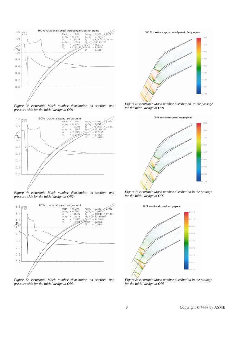
the surge-point Figures 3-5 show the isentropic Mach number distributions

on suction and the pressure sides of this airfoil for OP1, OP2 and OP3 respectively. Figures 6-8 show the isentropic Mach number distributions in the passage for the same operating-points. These results are calculated with the MISES-code [1] and will be discussed later.


Figure 3: isentropic Mach number distribution on suction- and pressure-side for the initial design at OP1



Figure 6: isentropic Mach number distribution in the passage for the initial design at OP1




The optimisation algorithm The optimisation strategy is based on multiobjective

evolutionary algorithms. Like every evolutionary algorithm it follows the example of nature that successful individuals can give their properties (their genes) to a next generation while unsuccessful individuals can‘t. Therefore after some generations only the suitable properties remain. In the context of evolutionary algorithms an individual is called a member and a conglomeration of members is called a population.

In this application of aerodynamic airfoil optimisation the genes of a specific member (here a specific airfoil) are determined by the design-parameters of the airfoil. The aim of the optimiser is to modify the values of these design-parameters to receive optimal solutions.

The basic algorithm is divided into two different phases which are almost the same for multi- and single-objective optimisation: the initialization and the iteration-loop. Initialization: The members of a start-population are initialised randomly. Thereafter these members are evaluated numerically and receive their objective values. Iteration: During the iteration-loop there are three different steps to be processed.

Selection: The algorithm chooses superior evaluated members to become possible parents of a new member (or a new population) Inheritance: With these parents a new member (or a new population) is created using different operators (Mutation, Crossover, Differential-evolution ...). Evaluation: The objective values of the new member (or all the members of a new population) are evaluated.

The only difference between multi-objective optimisation

and single-objective optimisation occurs in the selection-step. While the notation “superior member” in the selection-step is unique for single-objective optimisation with only one objective function f (M1 is “better” than M2 if w.l.o.g. f(M1)<f(M2) ), in the case of multi-objective optimisation the following two definitions are needed. Definition 1 Domination):Let f1,…,fk be the k-objectives of a multi-objective optimisation problem. Then a member M1 dominates a member M2

Definition 2 (Pareto-rank):The Pareto-rank of a member M is defined as

The Pareto-front is defined as

The probability for an evaluated member to become a

parent of a new member is given by the Pareto-rank. The aim of the multi-objective optimisation is to improve the Pareto-front and to reach a good diversity over the whole front. There are some verifications of this basic concept that are implemented in the optimisation-code that is used in this paper. The followings are the most important verifications: • Parallelization The optimisation-code is written in C and it is parallelized using MPI. Each new member is sent from the root-process to a specific slave-process where it passes through the process-chain. The objective-values are then calculated and returned to the root-process (see Figure 9). If several operating-points of the compressor are considered there is an inner loop over the number of operating-points added to the process-chain.

Figure 9: Flowchart of the optimisation-process • Normalization The free variables are normalized with their upper- and lower- limits. Therefore the optimisation kernel (the green module in Figure 9) is appropriate for each optimisation problem while the interface step in the process chain must rescale the normalized variables for the remainder of the process-chain. • Database Each evaluated member is stored in a database. If a metamodel like neural networks or kriging-models is used, the database contains the possible training-patterns for these models. The parents of a new member are also chosen from this database and not from the previous population like in traditional codes (see [3], [9], [10], [11]). The advantage of this approach is that it is natural to configure the algorithm asynchronous: The root process can select the possible parents for a new member without waiting until a whole population is passed through the process-chain.

A second advantage is that the diversity from the evaluated members over the whole front is easier to achieve especially for very complex and/or discontinuous fronts. An example for this is shown in Figure 10 for the ZDT 3 function with 30 free variables and 2 objectives (see [3]). The NASA-code needs a population size of 40 and 300 generations (all together 12000 members) to reach the exact front. The members are created

)()(:},...1{},...1{)()(

21

2121

MfMfkjkiMfMfMM

jj

ii

<∈∃∧∈∀≤⇔p

1}ˆ|ˆ{#:)( += MMMMemberevaluatedMP p

}1)ˆ(|ˆ{: == MPMMemberevaluatedPF


using the differential-evolution operator. However, the code used in this paper needs only 1100 evaluated members to reach the same front. If additive neural networks are used, this number can be reduced to 600 members without influencing the result. The main reason for this big difference is that traditional codes must ensure that each population spreads over the whole front and therefore a bigger population size is needed.

Figure 10: The ZDT3-function top: The NASA result; bottom: The DLR result • Asynchronous strategy The optimisation-process is asynchronous. That means each time the root-process receives the objective values of a slave, a new member is created and this new member is sent to the same slave process. Therefore there is no need to wait for the slowest member of a population to finish and results are obtained in optimal use of computational resources. • Similarity check Before a new member is sent to a slave, it is checked for similarity with all members in the database. The member is created new until this similarity-check fail. If too many similar new created members occur, the depth of the free variables will be increased. • Variable Parameter Depth The mathematical depth of the free variables is dynamic: In the initial phase of the optimisation process the computations are performed on a coarse grid of the search domain. That means the free variables can only get a small number of different values between their upper and lower limit. The grid is then gradually refined with convergence of the process in order to improve the accuracy of the final results. • Choosing parents This procedure is more complicate than in traditional codes. There is a fixed number of possible parents, NrPar, given in an

input file. At first all members of the database that have Pareto-rank 1 are selected as possible parents. This is noted as NrDom. 1. Case: NrDom > NrPar

If the number of dominating members NrDom is already bigger than NrPar there are two steps to process: -Reduce the whole Pareto-front successively to a specific region of interest in the objective space. (For example: concentrate in Figure 10 on the part of the Pareto front where 0.3<F1<0.5). This region of interest must be defined before the optimisation -One member of the most similar pair of possible parents (in parameter-space) is eliminated successively until NrPar is reached.

2. Case: NrDom < NrPar Until NrPar is reached the following steps are repeated: Built a tournament group randomly (each member of the database can be choosed) and select the member with the smallest Pareto-rank as an additional parent-member.

• Response-surface The algorithm searches for an approximation of the scatter plot given by the evaluated members in the database (points in the l+m dimensional space where l is the number of free variables and m is the number of objectives). This approximation is called a response-surface or a metamodel. For this approximation additive neural networks (see [8], [9]), Kriging procedures (see [5],[6]), MARS-algorithms (see [7]) and the hybridization of several of these models are used. When a metamodel is calculated (or trained) the optimisation runs temporarily on this approximation. The optimisation on a response-surface is very fast in comparison with an optimisation that uses a numerical expensive flow-solver particularly for 3D flow-simulations. Only the best members of the temporary optimisation on the response-surface are sent as new members, of the original optimization, to the slave processes. If the response surface is of a high quality it can accelerate the optimisation enormously. The biggest problem in building a response surface in high-dimensional spaces is known as the “curse of dimension” which is the depressing fact that the complexity of many problems depends exponentially on the dimension of the problem. The process-chain

The different modules of the process-chain for an aerodynamic optimisation are shown in Figure 9. These modules are almost the same for 2D airfoil and 3D compressor optimizations. The differences between 2D and 3D (e.g. for the geometry generator) are explained below. • Interface At the beginning the slaves must rescale the normalized variables corresponding to a received member to the real scaled variables needed by the Geometry Generator. • Geometry Generator The airfoils are constructed using B-Spline curves (for 3D blades B-Spline tensorproduct surfaces are used; see [2]). The most important input parameters are: -The axial length and the stagger angle, which are needed to transformate the airfoil from the unstaggered to the staggered system. -The leading-edge thickness, the leading edge angle, the wedge angle at the leading edge (same parameters for the trailing edge). With these parameters the first and the last control-


points for the B-Spline curves describing the suction and the pressure-side are calculated. -The other input parameters are (m’,Θ) coordinates of the remaining control points (the number of control points can vary between 5 and 9)for the suction and the pressure-side. The leading-edge and trailing-edge are calculated by interpolating B-Splines with a C2-connection to the neighbouring splines. At the end these 4 B-Splines are merged into a single B-Spline.

In 3D case several construction airfoils are created (in 2D) and transformed to 3D space (m’,Θ−transformation see [1]). After that a surface-skinning procedure calculates a B-Spline tensorproduct surfaces that exactly interpolates these construction airfoils.

The output of this mathematically closed description of the geometry is written in the step-format which can be read in by the most CAD-programs without an interpolation error. • Geometric restrictions With the design-philosophy described above it is possible to construct many different airfoils and to reconstruct almost any given airfoil. The disadvantage of design-philosophy is that most of these airfoils are unfeasible when the values of design parameters are choosen randomly (especially for a higher number of control-points). Therefore, it is important to check the airfoils for feasibility. For the optimisations in this paper the following geometric restrictions are used: 1. The maximal thickness (which is no input for the profilgenerator) of an airfoil must be in a given range. 2. Local minima in the thickness-distribution of an airfoil are forbidden because of structural requirements to a rotor blade.

3. The relation 7.0*max

>cld

PA must be valid

These conditions should ensure some rudimental sructural requirements of a rotor blade airfoil. If one of these conditions fails, the corresponding member gets bad objective values and is sent back to the root process immediately. However, the curvature distributions on the suction- and the pressure-side are not restricted. • Grid generator/flow-solver/post-processing In the current 2D case the iset grid generator, ises flowsolver and iplot post-processing programs were used. All of these programs are implemented in the MISES-package. For 3D applications all these modules are DLR-inhouse codes. Optimisation results

The following optimization results are calculated on a Linux-Cluster where 1 root and 29 slave-processes (each process on an own processor) are used. The initial airfoil is only used to estimate the upper- and lower limits for the design-parameters and not as an initial member of the optimisation. For both of the optimizations, the following conditions are valid:

-5 control-points on the pressure-side and 7 control-points on the suction-side are used to describe an airfoil. -All together there were 23 design-parameters choosen as free variables for the optimisation. -The ranges for the normalized maximum thickness dmax/cl are given by the interval [0.038, 0.044].

Optimisation 1 In a first attempt the original airfoil is optimized only for

the first operating point OP1.

From Figure 3 we can extract the reference values: ωref = 0.0744 β2,ref= 118.32 In this first optimisation only 1 objective-function F1 is used (single-objective) and is defined as:

ref

Fωω

=1 ; if ]5.0,5.2[ ,2,22 °+°−∈ refref βββ (1)

refref

F ,221 ββωω

−+= ; else. (2)

Thus the objective-value is given only by the losses as long as β2 is inside the tolerance-Interval (the interval in the above formula (1)). If β2 is outside of this Interval (bad conditions for the following stator) there is an additional penalty-term in the objective function (formula (2)). The tolerance-interval is asymmetric because a higher flow-turning might be necessary to increase the total pressure ratio for OP2 and OP3 (see Optimisation 2 below).

The optimisation was halted when 2000 members converged in the MISES calculations (without the use of a metamodel). This number can be reduced approximately to 1000 converged members, by the use of additive global trained neural networks. But for 2D aerodynamic optimisations the numerical effort to train the networks is bigger than the numerical effort to double the number of MISES calculations. With 29 slaves working simultaneously the optimisation needs approximately 45 minutes.

Figure 11: isentropic Mach number distribution on suction- and pressure-side for the optimised airfoil at OP1

Figures 11 and 12 show the MISES results of the dominating member. A comparison between Figures 11,12 and Figures 3,6 show that the shock on the optimized airfoil is shifted downstream and is more oblique than the shock on the initial airfoil. That’s the main-reason why the shock-losses could be reduced more than 2%, and the total pressure ratio was increased although the flow-turning was reduced.

A check of the aerodynamic behavior of this OP1-optimised airfoil at the other 2 operating points show, that the shock-losses and total pressure ratio for OP2 are improved (see Figure 4,13). However, the objective of increasing or


maintaining the total pressure ratio at OP3 failed for optimization 1 (see Figures 5 ,14). Moreover the shock structure for the aerodynamic design point (Figure 12) appears to have a swallowed shock while the initial geometry (Figure 6) did not. These drawbacks of the optimised geometry will be corrected by the approach of optimisation 2.

Figure 12: isentropic Mach number distribution in the passage for the optimised airfoil at OP1

Figure 13: isentropic Mach number distribution on suction- and pressure-side for the OP1-optimised airfoil at OP2

Figure 14: isentropic Mach number distribution on suction- and pressure-side for the OP1-optimised airfoil at OP3 Optimisation 2

Now the original airfoil is optimized for all three operating points. Therefore, two additional reference values are needed to define the objective functions (see Figures 4 and 5):

πt,ref 2 = 2.214 πt,ref,3 = 1.746

The first objective function F1 is defined as in optimization 1, while the other objective functions are defined as:

2,

2,,2

t

reftFπ

π=

3,

3,,3

t

reftFπ

π=

The region of interest in the objective space is defined as [0,1]³. That means we will concentrate on the region of the Pareto-front where:

-The losses for OP1 are smaller than ωref (and β2 is inside the interval of tolerance). -The total pressure ratio for OP2 is bigger than πt,ref 2 -The total pressure ratio for OP3 is bigger than πt,ref,3.

The dominating member of optimisation 1 for example is not in the region of interest because for this airfoil F3>1.

If a MISES calculation does not converge on any operating-point, the corresponding member gets bad objective-values for each objective-function and is returned to the root-process immediately.

Again the optimisation was halted when 2000 members converged in each of the 3 MISES calculations. Therefore optimization 2 takes approximately three times longer than optimization 1 to complete.

The final 3-dimensional almost convex Pareto-front consists of 80 dominating members with most of them inside the region of interest. Figures 15-17 show the Mach number distribution on suction- and pressure-sides of a member that was selected because it is a good compromise between the 3 objectives.


Figure 15: isentropic Mach number distribution on suction- and pressure-side for the MO-optimised airfoil at OP1 This multi-objective optimized airfoil dominates the initial one at each of the three operating-points. In OP1 the shock-losses are reduced about 2%, even though the shock-system in Figure 18 is not as favorable as the one in Figure 12. In OP2 and OP3 the total pressure ratio was increased significantly. To achieve this enhancement in total pressure, the multi-objective optimized airfoil must have a higher flow-turning than the OP1-optimised airfoil.

Figure 16: isentropic Mach number distribution on suction- and pressure-side for the MO-optimised airfoil at OP2

Figure 17: isentropic Mach number distribution on suction- and pressure-side for the MO-optimised airfoil at OP3

Figure 18: isentropic Mach number distribution in the passage for the MO-optimised airfoil at OP1

Conclusions and future works

This paper introduced an automated multiobjective design methodology for the aerodynamic optimisation of turbomachinery airfoils. It was shown that the consideration of several operating-points is essential to improve the aerodynamic behaviour for the whole working range of a compressor. An alternative evolutionary algorithm was introduced which is capable to improve the flow-characteristics significantly within an acceptable time.

In future works we will expand this approach to 3D compressors with more several blade rows. The automated 3D process-chain is already set up but it is still an aim to reduce the

numerical effort by improving the quality of the metamodels in high dimensional spaces.

REFERENCES [1] Drela, M., Youngren, H. , 1998, “A User’s guide to Mises”, MIT Computational Aerospace Sciences Laboratory. [2] Piegl, L., Tiller, W., 1997, “The Nurb’s book”, Monographs in visual communication, Springer, ISBN 3-540-61545-8. [3] Rai, M., November 2004, “Multiple-Objective Optimization with Differential Evolution and Neural Networks”, NASA Ames Research Centre, VKI Lecture-Series.


[4] Kügeler, E., Weber, A., Lisiewicz, S., 2001, “Combination of a Transition Model with a Two-Equation Turbulence Model and Comparison with Experimental Results”, Proc. 4th Eu. Conf. TurbMach, ATI-CST-076/01, Florence, Italy. [5] Sacks, J., Welch, W. J., Mitchell, T. J., Wynn, H. P., 1989, “Design and analysis of computer experiments”, Statistical Science, 4, 409-435. [6] Welch, W. J., .Mitchell, T. J., Wynn, H. P., 1992, “Screening predicting and computer experiments”, Technometrics, 34 (1), 15-25. [7] Friedman, J. H., 1991, “Multivariate adaptive regression splines”, Anals of Statistics 19: 1441. [8] Faller, W., Schreck, S., 1996, “Neural Networks: Applications and opprtunities in aeronautics”, Progress in aerospace sciences, 32, 433-456. [9] Giannakoglou, K., C., November 2004, “Neural network assisted Evolutionary algorithms in aeonautics and turbomachinery”, VKI Lecture-Series. [10] Van den Braembussche, R., A., November 2004, „Fast multidisciplinary optimisation of turbomachinery components”, VKI Lecture-Series. [11] Ahmed, R., Lawerenz, M., 2003, “On the aero-mechanical design of multistage axial compressors using parallel optimisation algorithms”, 16’th Symposium on air breathing engines, Number ISABE 2003-17. [12] Benini, E., 2004, “Three-dimensional multi-objective design optimisation of a transonic compressor rotor”, Journal of propulsion and power, 20, 559-565. [13] Drela, M., Youngren, H., 1991, “Viscous/Inviscid Method for Preliminary Design of Transonic Cascades”, AIAA Paper 91-2364, Sacramento, CA, USA.

automated multiobjective optimisation in axial compressor

Documents