automated model generation for hybrid vehicles

Oil & Gas Science and Technology – Rev. IFP, Vol. 65 (2010), No. 1, pp. 115–132Copyright c© 2010, Institut français du pétroleDOI: 10.2516/ogst/2009064

Automated Model Generation for Hybrid VehiclesOptimization and Control

N. Verdonck, A. Chasse, P. Pognant-Gros and A. Sciarretta∗

Institut français du pétrole, IFP, 1-4 avenue de Bois-Préau, 92852 Rueil-Malmaison Cedex - Francee-mail: [email protected] - [email protected] - [email protected] - [email protected]

∗ Corresponding author

Résumé — Création automatique de modèles de composants pour l’optimisation et le contrôle devéhicules hybrides — L’optimisation de l’utilisation des groupes moto-propulseurs (GMP) modernesnécessite de modéliser le système de manière quasi-statique avec une logique inverse (“Backward Qua-sistatic Model’’ – BQM), en particulier dans le cas des GMP hybrides. Cependant, les modèles utiliséspour la simulation réaliste de ces GMP sont souvent dynamiques à logique directe (“Forward DynamicModel’’ – FDM). Cet article présente une méthodologie pour obtenir les BQM des composants de GMPactuels directement issus de la limite quasi-statique des FDM correspondants de manière analytique.Grâce à l’aspect paramétrique de cette procédure, il n’est pas nécessaire de relancer une campagnede simulations après chaque changement du système modélisé : il suffit de modifier les paramètrescorrespondants dans le BQM. Cette approche est illustrée par trois cas d’étude (moteur turbo, moteurélectrique et batterie), et l’effet d’un changement de paramètre sur le contrôle de supervision d’unvéhicule hybride est étudié en simulation hors-ligne, en co-simulation et sur un banc d’essai HiL adaptéaux architectures hybrides (HyHiL).

Abstract — Automated Model Generation for Hybrid Vehicles Optimization and Control — System-atic optimization of modern powertrains, and hybrids in particular, requires the representation of thesystem by means of Backward Quasistatic Models (BQM). In contrast, the models used in realisticpowertrain simulators are often of the Forward Dynamic Model (FDM) type. The paper presents amethodology to derive BQM’s of modern powertrain components, as parametric, steady-state limitsof their FDM counterparts. The parametric nature of this procedure implies that changing the systemmodeled does not imply relaunching a simulation campaign, but only adjusting the correspondingparameters in the BQM. The approach is illustrated with examples concerning turbocharged engines,electric motors, and electrochemical batteries, and the influence of a change in parameters on thesupervisory control of an hybrid vehicle is then studied offline, in co-simulation and on an HiL testbench adapted to hybrid vehicles (HyHiL).

Advances in Hybrid PowertrainsÉvolution des motorisations hybrides

IFP International ConferenceRencontres Scientifiques de l’IFP

http://ogst.ifp.fr/

http://www.ifp.fr/

http://ogst.ifp.fr/index.php?option=toc&url=/articles/ogst/abs/2010/01/contents/contents.html

http://ogst.ifp.fr/index.php?option=toc&url=/articles/ogst/abs/2010/01/contents/contents.html

116 Oil & Gas Science and Technology – Rev. IFP, Vol. 65 (2010), No. 1

NOMENCLATURE

A{in;exm;exh} External surface: intake manifold, exhaust manifold, exhaust pipeC{e;tc;m} Torque: engine, turbocharger, motor

Cq,{tv;he,eq;wg;exh,eq} Discharge coefficient: throttle, exchanger (equivalent), waste gate, exhaust pipe (eq.)

cp,{a;exh} Constant pressure specific heat: air, exhaust

C{Ni;MH} Concentration: nickel, metal hydride

D Mass flow rate through the engine

D{in j;exh;t;t,corr;wg} Mass flow rate: injector, exhaust, turbine, turbine (corrected), waste gate

h{exm;exh} Conductive heat exchange coefficient: exhaust manifold, exhaust pipe

H{in;exm;exh} Convective heat transfer coefficient: intake manifold, exhaust manifold, exhaust pipe

I{d;dt;q;qt} Current: direct, direct (transferred), quadrature, quadrature (transferred)

I{m;m,max;b} Current: motor, motor (maximum), battery

k{Ni;MH} Electrode parameter: nickel, metal hydride

Ls Stator inductance

mair Inducted air mass

N{e;tc;tc,corr} Rotational speed: engine, turbocharger, turbocharger (corrected)

ncell No. of battery cells

p Number of pole pairs

p{in;c;e} Pressure: intake manifold, compressor exit, exchanger exit

p{exm;t;0} Pressure: exhaust manifold, turbine exit, ambient

P{m;m,max;b} Electric power: motor, motor (maximum), battery

Q{ f ;exm} Fuel lower heating value, heat flow at the engine exhaust

R{a;s;i;cell} Gas constant, resistance: serial, parallel, battery cell

S {tv;tv,max;wg;wg,max} Cross section: throttle, throttle (maximum), waste gate, waste gate (maximum)

S {he,eq;exh,eq} Cross section: exchanger (equivalent), exhaust pipe (equivalent)

T{in;a,in;c;e} Temperature: intake manifold, intake manifold (air), compressor exit, exchanger exit

T{exm;s,exm;s;s,exh} Temperature: exhaust manifold, exh. manifold (surface), exh. pipe, exh. pipe (surf.)

T{t;re f ,t;tb} Temperature: turbine exit, turbine (reference), turbine (main flow exit)

T{0;cool} Temperature: ambient, coolant

U{d;q;b;oc;re f } Voltage: direct, quadrature, battery, open circuit, reference

Ved Engine displacement

x Auxiliary variable

ε{a;exh} Compression factor: air, exhaust(εi =

γi−1γi

)η{v;ind;c;exm;t;m} Efficiency: volumetric, global (fuel–torque), fuel–exhaust, compressor, turbine, motor

ϕm Magnetic flux

Π{c;t} Pressure ratio: compressor, turbine

ω Rotational speed: motor

ξ Battery SOC

INTRODUCTION

Hybrid propulsion systems are nowadays increasingly rec-ognized as one of the few possibilities of combining lowCO2 emissions, acceptable range, and good performance inroad vehicles. In spite of their complexity with respect toconventional powertrains, hybrids offer additional degreesof freedom that can be optimized.

Optimization of hybrid energy management (supervisorycontrol) ensures that the hybrid operation along, e.g., a drivecycle, is optimal with respect to some dynamic criterion.Such criterion is typically related to energy consumption andsubjected to several constraints. On the other hand, optimaldimensioning consists of selecting the best choice in terms

of components. If the same criteria are used, the simultane-ous optimization of both task is possible (co-optimization,see Rousseau et al., 2008; Sundström et al., 2008).

The optimization and control of hybrid powertrains isincreasingly based on system modeling in contrast to heuris-tic strategies dictated by experience only. Although model-based techniques are inherently more flexible than heuris-tic strategies, however often they are still structured fora specific hybrid architecture. The literature offers sev-eral examples concerning parallel hybrids but also seriesand combined hybrids (see the comprehensive survey inSciarretta and Guzzella, 2007). Many of these examplesdevelop a control law (ECMS) based on the formulationof an optimal control problem. However, this formula-tion depends on the specific hybrid architecture. Such a

N Verdonck et al. / Automated Model Generation for Hybrid Vehicles Optimization and Control 117

constraint makes difficult studying the impact of the archi-tecture on the energy consumption and performance. More-over, a control structure developed for one architecture ishardly reusable for different ones.

Thus it would be beneficious to explore the possibilityof deriving a generic model-based control structure for anytype of hybrid powertrain. That structure would enable para-metric studies and co-optimization of the powertrain con-figuration, not only of the component characteristics. Alsoreusability of data and results from one hybrid applicationto another would be enhanced.

Key factors for pursuing such a program are: (i) a genericsystem model, which is able to represent several config-urations using the same set of equations belonging to theclass of Backward Quasistatic Models (BQM) (1) used inoptimization, (ii) a generic control structure emerging fromthe harmonization of different ECMS algorithms and capa-ble of dealing with a generic BQM, (iii) a dedicated testingtool that is able to experimentally represent various hybridarchitectures.

Concerning (i), a generic optimization-oriented model isused in the software tool HOT (Hybrid Optimization Tool),developed at IFP (Chasse et al., 2009b). With regard to (ii),the equivalence of the ECMS with Pontryagin’s MinimumPrinciple (PMP, Serrao et al., 2009) ensures that the coreof HOT can be used as an online controller (Chasse et al.,2009b), which thus profits of the same generality as HOT’ssystem model.

As for (iii), a solution that is implemented at IFP impliesthe use of the Hardware-in-the-Loop (HiL) concept. Inthis HiL hybrid test bench (HyHiL), the power provided orabsorbed by the hybrid components (motors, battery, etc.)is physically emulated. This emulation is made possiblethanks to dynamic models of the hybrid components thatrun in real time in the system control hardware (Del Mastroet al., 2009). It should be noticed that these models arenot BQM’s, but rather they belong to the class of ForwardDynamic Models (FDM), which differ from the BQM withrespect to causality and temporal resolution (Guzzella andSciarretta, 2007). With the help of a library of such models,it will be possible to change the hybrid architecture undertest. The controller should then automatically adapt accord-ing to the steps (i)–(ii) mentioned above thanks to its genericstructure.

Ensuring that the FDM’s used to emulate the hybrid pow-ertrain and the corresponding BQM’s used in the controllerare always consistent with each other is an important and alittle studied problem. To cope with that, the simplest solu-tion consists of launching a simulation campaign for eachsystem represented (Murgovski et al., 2008). The FDM of

(1) A library of BQM’s called QSS is publicly available for academicpurpose at the URL http://www/imrt.ethz.ch/research/qss/. See alsoGuzzella and Amstutz (1999).

the system should be run for every combination of the oper-ating conditions in order to Build Quasistatic Maps (BQM)point-by-point. The disadvantage of such a technique isthat there are virtually as many maps as the combinationsof system parameters. For such a reason, artificial neuralnetworks have been adopted in similar problems, e.g., byDelagrammatikas et al. (2004).

An alternative methodology consists of deriving theBQM’s as parametric, steady-state limits of their dynamiccounterparts. Each FDM is defined by parameters (dimen-sioning, coefficients, maps, etc.) that affect the equationsrepresenting the behavior of the system modeled. Thesteady-state behavior can be sought by letting the dynamicsvanish in the system of differential equations constitutingthe model. The solution of such steady-state system is theBQM sought. It will be parametric, i.e., it will depend ona subset of the parameters of the FDM. Thus changing themodeled system does not imply relaunching a simulationcampaign, but only adjusting the corresponding parametersin the BQM.

The proposed method is applicable to any component ofmodern powertrains for which a consolidated dynamic mod-eling technique exists. After having introduced FDM’s andBQM’s in Section 1, and the associated tools in Section 2,the paper presents developments concerning naturally-aspirated and turbocharged engines (Sect. 3) as well as elec-tric motors and electrochemical batteries (Sect. 4). In Sec-tion 5 simulation and experimental results are illustrated anddiscussed.

1 FDM AND BQM FOR HYBRID POWERTRAINS

Different classes of models are usually used in real-timesimulation and control of modern powertrains. Among sev-eral other characteristics, they mainly differ with regard to(i) causality and (ii) temporal resolution.

With respect to the causality, a distinction is often madebetween forward and backward models. Recall that in mod-ular modeling, each component of the system is simulatedas a stand-alone subsystem, which exchanges variables withthe other subsystems through connectors. Typical connec-tors are pairs of power factors (e.g., torque and speed, cur-rent and voltage, etc.). Connectors are non-causal whenall physical effects are described only with equations orother relationships, without any input/output prescription.However, in many applications connectors are causal, whichmeans that input and output variables have to be assignedat each connector (2). With respect to the philosophy thatinspires the choice of the inputs and outputs, backward mod-eling assigns both the power factors at a single connector as

(2) Modelica/Dymola is an example of a simulation environment based onnon-causal connectors, while Simulink or AMESim are examples ofsimulation environments of the causal type.


Figure 1

Forward and backward causality patterns for an engine system.

inputs or outputs. In contrast, in forward modeling at eachconnector one power factor is selected as an input, the otheras an output. Examples of forward and backward causalityfor an internal combustion engine are illustrated in Figure 1.

As for the model temporal resolution, the key distinctionlies between quasistatic and dynamic models. The formerclass does not contain state variables, and all the dependen-cies between variables are intended to be the same as in thecase of steady state.

The performance of a powertrain and its controllersalong a prescribed drive cycle is conveniently assessedusing the Backward Quasistatic Modeling (BQM) approachin which the flow of input variables is directed from theend of the propulsion chain (the wheels) toward the primemovers (the engine). Although internal powertrain dynam-ics are neglected, the overall prediction can be very accurate(Guzzella and Amstutz, 1999). The BQM approach is alsonaturally suitable in powertrain control. Indeed, the “torquecontrol’’ structure of modern powertrains, including hybridpowertrains, is such that at each time the driveline speedcan be measured while the torque demand is estimated fromthe accelerator pedal using several mappings. Then, follow-ing the propulsion chain backwards, the torque and speeddemand can be predicted, e.g., at the output stage of theengine.

On the other hand, Forward Dynamic Modeling (FDM)finds its natural place in system simulators. Not only theforward causality can represent the internal dynamics of thesystem, but it also well represents the cause-and-effect rela-tionships, enlightening the effect of the control variables onthe instantaneous powertrain performance. A consequenceof this approach is that the vehicle speed must be calculatedas a function of the other power factor, namely, the tractionforce. Therefore, in order to follow a prescribed drive cycle,a model of a ‘driver’ is needed to demand more or less powerto the prime movers.

A hierarchical structure illustrating the role of FDM’sand BQM’s in powertrain simulation and control as well astheir interactions is shown in Figure 2. The figure clearlydistinguishes quasistatic models, while dynamic models canhave very different temporal resolutions. Two main classes

Figure 2

Hierarchical structure of FDM and BQM interactions.

are recognizable according to their relationships with con-trollers. Component controllers (e.g., engine controllers,motor controllers, etc.) are usually based on dynamic mod-els with a medium-frequency temporal resolution. The val-idation of such controllers is thus necessarily entrusted tohigher frequency models.

As an example, in internal combustion engines themedium-frequency class is represented by the well-knownMean-Value Engine Models (MVEM), which have a tem-poral resolution of one engine cycle. Engine controllersare more and more based on MVEM’s (air loop control,fuel loop control, etc.). In contrast, high-frequency mod-els of engines typically have a temporal resolution of oneor few crank angles, thus representing the dynamics insidethe cylinders, etc. Similar considerations apply for motors,batteries, and other components of modern powertrains.

In contrast to component-level controllers, powertrain-level controllers are based on quasistatic models, see Fig-ure 2, and thus their validation necessitates FDM’s of theMVEM type. Ensuring that the FDM used to emulate thehybrid powertrain and the corresponding BQM used in thecontroller are always consistent with each other is an impor-tant and a little studied problem.

The methodology illustrated in the following sectionsconsists of deriving the BQM using two steps. In a first step,the steady-state behavior of the FDM is sought by lettingits dynamics vanish in the system of differential equationsconstituting the model. The resulting model is quasistaticbut still with the forward causality (FQM). Its role here isto determine the admissible inputs for the BQM, which isderived in a second step by changing the causality.

Notice that both the FQM and the BQM will be paramet-ric, i.e., they will depend on a subset of the parameters of theoriginal FDM. Thus changing the modeled system does notimply relaunching a simulation campaign, but only adjust-ing the corresponding parameters in the FQM and BQMgeneration.


Figure 3

Tool chain for hybrid control development based on the hierar-chical modeling structure of Figure 2.

Figure 4

Schematic representation of the HyHiL setup for a hybrid pow-ertrain.

2 TOOLS

The generic hierarchical modeling structure of Figure 2reveals the importance of the model generation process,which is described by the arrows pointing from FDM’s toFQM’s and then to BQM’s. While the rest of the paper willpresent some examples of such a model generation, this sec-tion shows how the various modeling levels are integratedinto a chain of tools for control design and prototyping, seeFigure 3.

The QM’s are used for real-time model-based supervi-sory control as well as for offline optimisation. The offlineoptimization stage consists of calculating the evolution ofpowertrain power factors along a prescribed drive cycle,that are optimal with respect to some mathematical crite-rion (typically, the minimization of the fuel consumptionover the cycle). The software tool named HOT, developedand validated at IFP (Chasse et al., 2009b) uses BQMs(static maps) to represent the powertrain components anda generic model structure to represent various hybrid con-figurations. Unlike other offline optimisation tools, whichmostly apply Dynamic Programming techniques (Rousseauet al., 2008; Sundström et al., 2008; Scordia et al., 2005),HOT is based on the Pontryagin minimum principle, i.e.,on the direct application of the optimal control equations(Rousseau et al., 2007; Serrao et al., 2009). In the nextfuture, HOT will integrate an automated QM generation pre-processor in order to build the necessary static maps frommean value models (FDM’s).

Online supervisory control are also more and more basedon modeling and optimisation. The ECMS controller devel-oped at IFP (Chasse et al., 2009a) use BQM’s as in offlineoptimisation to calculate the optimal control outputs. Inorder to validate an ECMS controller, a first approach is tocontinuously send the control outputs to a real-time runningpowertrain simulator. As shown in Figure 3, this simulator

must be based on mean-value FDM’s to ensure a fair val-idation of the supervisory controller. Such a procedure isknown as co-simulation and it is often preliminary to thevalidation of the controller on a real system.

As a final step of the control prototyping chain, theECMS-based controllers are integrated in a testing conceptfor hybrid powertrains called HyHiL. This concept couplesa real engine test bench with FDM’s running in real timethat emulate the transmission chain as well as the hybridcomponents (e.g., battery, electric motor, power electron-ics, etc.). Unlike similar engine-in-the-loop concepts (Filipiet al., 2006; Jeanneret et al., 2004), high-frequency modelsare used for the drivetrain and hybrid components. The goalof the HyHiL concept is to test a component at a time in anenvironment that realistically represents a hybrid powertrainincluding drivability issues. As depicted in Figure 4, theengine test bench is controlled in such a way that the speedand the torque at the engine output shaft represent the out-come of a driver request (e.g., to follow a drive cycle) and theoutput of the supervisory controller that splits such a requestbetween the engine and the electric motor(s). Similarlyto the co-simulation scenario, the ECMS controller needsBQM’s for the physical engine as well as BQM counterpartsof the FDM’s emulating the hybrid drivetrain.

3 AUTOMATED QM GENERATION FOR ENGINES

3.1 Naturally-Aspirated EnginesThis section illustrates the method of generating a BQM fora naturally-aspirated engine with the purpose of presentingsimple developments that will be later extended to morecomplex engine systems. Since mean-value modeling ofengines is an established technique (Guzzella and Onder,2004), the relevant equations will be listed below withoutfurther comments on their derivation.


Figure 5

Connections between submodels of a naturally-aspiratedengine.

3.1.1 Equations

The main submodels of a naturally-aspirated engine are con-nected as in Figure 5. For each of the submodels, thestatic equations describing its steady-state, mean behaviorare extracted from the corresponding FDM. For the meaningof the variables, refer to the nomenclature.

Throttle Valve

The air mass flow rate through the throttle valve is given bythe nozzle equation (3)

D =S tvCq,tvP0√

T0Cm

(Pin

P0

)(1)

The quasistatic hypothesis implies that the mass flow rate Dis constant along the air path.

Intake Manifold

The temperature in the intake manifold is calculated from anenergy balance,

Dcp,a(Tin − T0) = AinHin(Ta,in − Tin) (2)

Cylinders

The intake mass flow rate is usually expressed in terms ofvolumetric efficiency that is often parameterized as a func-tion of intake pressure and engine speed,

D =Pin

RaTinηv(Pin,Ne)

Ne

4πVed (3)

Likewise, the torque generation is represented by an indi-cated efficiency map as a function of air mass and enginespeed. Pumping losses are also considered to obtain theeffective (shaft) torque,

Ce =1

Ne

(ηind (mair,Ne) Q f Din j − Ne

4πVed (P0 − Pin)

)(4)

(3) Also known as the Barré de Saint-Venant equation.

The air mass inducted in one cylinder is related to massflow rate through the equation

mair =4πDNe

(5)

Moreover, fuel consumption Din j is proportional to D ormair, considering a fixed air to fuel ratio.

3.1.2 Resolution

Besides the constant parameters (eleven) and the tabulateddata (two maps), Equations (1-5) contain seven unknowns(D, S tv, Ne, Ce, mair , Pin, Tin). If two of the unknownsare imposed, the other five variables can be solved for. Inthe FQM, S tv and Ne are imposed. In the BQM, the torquesetpoint Ce and Ne are imposed.

The solution procedure is detailed in Appendix both forthe FQM and the BQM.

An example output of the FQM generation is the graph inFigure 6, where the torque curves for several throttle com-mands are shown. These curves explicitly yield the maxi-mum and minimum engine torque, which will be used laterin the BQM generation to saturate the torque input.

An example output of the BQM generation is the graph ofFigure 7, showing a Din j map obtained by solving the pro-cedure above for several admissible torque and speed values(saturated with respect to the output curves of the FQM).

3.2 Turbocharged Engines

Mean-value modeling of turbocharged engines is a well-known technique that is also frequently adopted as a basisfor model-based control. See Müller et al. (1998), Moraalet al. (1999), Eriksson (2007) for further details.

Figure 6

Torque curves as a function of the throttle valve command andengine speed for a naturally-aspirated engine.


Figure 7

Fuel consumption map of a naturally aspirated engine.

3.2.1 Equations

The main submodels of a turbocharged engine are connectedas in Figure 8. For each of the submodels, the static equa-tions describing its steady-state, mean behavior are extractedfrom the corresponding FDM.

In the following, nozzle equations will be denoted by thefunction BSV defined as

BS V(S ,Cq, Pup, Pdown, Tup) =S CqPup√

Tup

Cm

(Pdown

Pup

)(6)

Compressor

The compressor behavior is described by static maps andfirst-principle equations. The characteristic curve mapyields

Pc = P0 Πc(D,Ntc) (7)

while an isentropic efficiency map is used to calculate down-stream temperature as

Tc = T0

(1 +Πc(D,Ntc)εa − 1ηc(D,Ntc)

)(8)

Moreover, the compressor torque is calculated using energybalance,

Ctc =D

Ntccp,a(Tc − T0) (9)

Heat Exchanger

Heat exchangers are variously simulated in FQM’s. A possi-ble choice is with the assumption of several pressure lossesin series representing connecting pipes and the exchanger

itself. Here a lumped equivalent pressure loss is consideredin such a way that

D = BS V(S he,eq,Cq,he,eq, Pc, Pe, Tc) (10)

Also, it is assumed that at steady state the temperature ofair downstream of the exchanger equals the temperature ofthe coolant that is given by the map

Te = Tcool(Ne,Ce) (11)

Throttle Valve, Intake Manifold, Cylinders

The models of the throttle valve, the intake manifold, and thecylinders are the same as in the naturally-aspirated enginemodel, except for the fact that Pe, Te replace P0 and T0 atthe inlet of the throttle, while Pexm replaces P0 at the outletof the cylinders. Thus

D = BS V(S tv,Cq,tv, Pe, Pin, Te) (12)

Dcp,a(Tin − Te) = AinHin(Ta,in − Tin) (13)

D =Pin

RaTinηv(Pin,Ne)

Ne

4πVed (14)

Ce =1

Ne

(ηind(mair,Ne)Q f Din j − Ne

4πVed(Pexm − Pin)

)(15)

and Equation (5) holds for mair.

Figure 8

Connections between submodels of a turbocharged engine.


An additional equation is now necessary to find the tem-perature at the exhaust, Texm, which is done with a thirdengine map (besides ηv and ηind) representing the heat fluxto the exhaust,

Qexm = ηexm(mair,Ne)Q f Din j (16)

Exhaust Manifold

The exhaust temperature is found from an energy balanceapplied to the exhaust manifold involving a variable walltemperature and neglecting the radiating contribution,

Texm =

Dcp,aTin + Qexm + AexmhexmHexm

Hexm + hexmTs,exm

Dexhcp,exh + AexmhexmHexm

Hexm + hexm

(17)

The mass flow rate through the exhaust manifold isDexh = D + Din j.

Turbine

The turbine behavior is described by static maps and first-principle equations. The characteristic curve map yields

Dt =Dt,corr(Πt,Ntc,corr)√

TexmPexm (18)

where Πt = Pexm/Pt and Ntc,corr = Ntc√

Tre f ,t/Texm.Downstream temperature is calculated using an isen-

tropic efficiency map

Ttb = Texm

(1 − ηt(Πt,Ntc,corr) ·

(1 − Π−εexh

t

))(19)

Moreover, the turbine torque is given by

Ctc =Dt

Ntccp,exh(Texm − Ttb) (20)

The mass flow rate through the waste gate is calculatedwith the nozzle equation,

Dwg = BS V(S wg,Cq,wg, Pexm, Pt, Texm) (21)

The sum of the mass flow rate through the waste gate andthrough the turbine gives the total mass flow rate at exhaust,

Dexh = Dwg + Dt (22)

Downstream of the turbine, the mass flow coming fromthe turbine and the waste gate mix together into a single flow,whose temperature is given by

Tt =DtTtb + DwgTexm

Dexh(23)

Exhaust Pipe

The mass flow rate through the pipe is calculated with thenozzle equation,

Dexh = BS V(S exh,eq,Cq,exh,eq, Pt, P0, Tt) (24)

The exhaust temperature is found from an energy balanceapplied to the exhaust pipe involving a variable wall temper-ature and neglecting the radiating contribution,

Ts =

Dexhcp,exhTt + AexhhexhHexh

Hexh + hexhTs,exh

Dexhcp,exh + AexhhexhHexh

Hexh + hexh

(25)

3.2.2 Resolution

Besides the constant parameters and tabulated data, the 20Equations (7-24) contain 23 unknowns. Thus if three of theunknowns are imposed, the other twenty variables can besolved for. In the FQM, S tv, S wg, and Ne are imposed. In theBQM, Ce and Ne are imposed together with the additionalconstraint on the values of S tv and S wg, that

S wg = S wg,max if S tv � S tv,max (26)

The resolution procedure is described in Appendix.Example outputs of the FQM and BQM generation are thetorque curves of Figure 9 and the fuel consumption map ofFigure 10. Notice that the maximum torque curve visible inFigure 10 can be easily extracted from the data in Figure 9by enveloping the maxima of the torque curves at variousthrottle or waste gate commands.

Figure 9

Torque curves of a turbocharged engine as a function of thethrottle valve command (0-100) and the waste-gate command(100-200), as well as the engine speed.


Figure 10

Fuel consumption map of a turbocharged engine.

4 AUTOMATED QM GENERATION FOR HEV

4.1 Electric Machines

In this section, the approach illustrated for engines is appliedto a different component of EVs and HEVs, i.e., elec-tric motors. This development considers only one type ofmotors, namely, the Permanent Magnet Synchronous Motor(PMSM).

4.1.1 Equations

Similarly to other types of motors, FDM’s of PMSM arebased on the electric circuit approach representing themachine characteristics as lumped electric parmaters suchas resistances, inductances, etc. The equivalent circuit of aPMSM with iron losses is depicted in Figure 11 (Sun et al.,2008; Urasaki et al., 2000).

The steady-state equivalent circuit equations yield

Ud = RsId − pωLsIqt = RsId + Ri(Id − Idt) (27)

Uq = RsIq + pω(LsIdt + ϕm) = RsIq + Ri(Iq − Iqt) (28)

Figure 11

Equivalent electrical circuits of a PMS Motor (ωe � pω).

Cm = pϕmIqt (29)

In absence of iron loss, Id = Idt and Iq = Iqt

4.1.2 Resolution

The five Equations (27-29) contain eight unknowns (Ud, Uq,Id, Iq, Idt, Iqt, Cm, ω), besides the constant parameters. Bothin the FQM and in the BQM, only two variables have tobe imposed, thus one equation is still necessary to solve thesystem. This missing equation describes the motor controlstrategy.

In Maximum Torque per Ampere (MTA) control(Mohamed and Lee, 2006), the torque is maximized withrespect to Id and Iq with the constraint that I2

q + I2d = I2

m. Forthe system under study, this strategy leads to

Id = −ωLs

RiIq � −x(ω)Iq (30)

regardless of the value of Im.Therefore it is possible to calculate the quasistatic dq cur-

rent and voltage as a function of motor torque and speed,which are imposed in the BQM,

Iqt =Cm

pϕm(31)

Iq = Iqt +x

1 + x2

ϕm

Ls(32)

Idt = − x2

1 + x2

ϕm

Ls(33)

The electric power Pm = UdId+UqIq, i.e., the output variableof the BQM, is calculated as

Pm = ωCm +xω

1 + x2

ϕ2m

Ls+

[Rs(1 + x2) + Rix2

]·

·(C2

m

ϕ2m+

( x1 + x2

)2 ϕ2m

L2s+

2x1 + x2

Cm

Ls

) (34)

from whence the efficiency ηm = ωCm/Pm follows. Thequasistatic modeling is completed by the physical limitsimposed on the electric power Pm < Pm,max and on thecurrent Im < Im,max, which impose a limit to torque that isvariable with speed.

4.2 Batteries

Batteries are often represented in system-level simulators ina quasi-static way as simple equivalent circuits, like in Fig-ure 12. The equivalent electric circuit comprises a voltagesource and a resistance, both varying with the state of chargeand temperature. In contrast, battery dynamics is variouslyrepresented. FDM of automotive batteries range from black-box or ‘gray-box’ equivalent circuit models (Kuhn et al.,2006; Takano et al., 2000) that try to reproduce batterydynamics with networks of resistances and capacitances,to electrochemical models (Newton and Paxton, 1997; Wuet al., 2001; Botte et al., 2000; Zhang and White, 2007).


Figure 12

Simple equivalent circuit of an automotive traction battery.

4.2.1 Equations

In Bernard et al. (2008), a lumped-parameter electrochem-ical model has been presented for Ni-MH batteries, whichcomprises among the state variables the concentrations ofthe reactant species and the electrode reference potentials,while the State Of Charge (SOC) is calculated from thenickel concentration. Neglecting the influence of the sidereactions (involving the production or absorption of gaseousoxygen) that are relevant only for high values of SOC, andother dynamic effects, a simplified cell FDM consisting offour equations is derived as⎧⎪⎪⎪⎪⎪⎪⎨⎪⎪⎪⎪⎪⎪⎩

Ure f = f (Ure f , s)Ub = g(CNi,CMH , Ib,Ure f , Tb)CNi = kNiIb

CMH = −kMH Ib

(35)

where Ib is the cell output current (positive if discharging),s = sign(Ib), Ub is the output voltage of the battery cell, Ure f

is the reference potential of the nickel electrode, CNi andCMH are the nickel and the metal hydide concentrations, Tb

is the temperature, and f (·), g(·) are nonlinear functions thatdepend on many electrochemical and geometrical parame-ters, as the constants kNi and kMH do. The cell SOC is

ξ = 1 − CNi

CNi,max(36)

A static counterpart of the first two equations of theset (35) can be extracted as

Ub = g(CNi,CMH , Ib,U∞re f (s), Tb) (37)

with U∞re f (s) s.t. f (Ure f , s) = 0. Conversely, the SOCdynamics is that of a pure integrator and in such a way itcannot generate static equations. Instead, the SOC is relatedto CNi through Equation (36), while the concentration CMH

is related to CNi via the balance of total number of moles,kNiCMH + kMHCNi = const. Consequently, Equation (37)reduces to

Ub = h(ξ, Ib, Tb) (38)

where

ξ = − kNiIb

CNi,max(39)

The latter equation compares with the well-knownCoulomb-counting equation that is the baseline to estimatethe SOC online. The term CNi,max/kNi is equivalent to thenominal battery capacity.

4.2.2 Resolution

The set of Equations (35) has six unknowns. Thus if twoof the unknowns are imposed, the other four variables aresolved for. In both FQM and BQM, the temperature Tb canbe treated as an input (exogeneous variable). Moreover, inthe FQM the current Ib is imposed, while in the BQM theelectric power Pb = IbUb is imposed. In order to solveEquation (38) in terms of Pb in closed form, the equiva-lent circuit approximation of Figure 12 is introduced. Thecell parameters Uoc and Rcell are derived by linearizing thefunction h(·) around a current I0,

Ub ≈ h(ξ, Tb, I0) +∂h∂Ib

∣∣∣∣∣I0

· (Ib − I0) (40)

Since U∞re f depends on the sign of the current, h(·) is lin-earized twice, for ±I0. This expression yields two values ofUoc and Rcell for the equivalent circuit, according to s that isalso the sign of the power Pb,⎧⎪⎪⎨⎪⎪⎩Uoc(ξ, Tb, s) = h(ξ, Tb, sI0) − ∂h

∂I

∣∣∣sI0· sI0

Rcell(ξ, Tb, s) = ∂h∂I

∣∣∣sI0

(41)

Therefore the linearization parameters that do not dependon Ib, thus the battery BQM can be solved from the equiv-alent circuit equations including the number of cells inseries ncell,

Ib =Uoc

2Rcell−

√(Uoc

2Rcell

)2

− Pb

ncellRcell

Ub =ncellUoc

2+

√(ncellUoc

2

)2

− ncellRcellPb

(42)

Moreover, a battery local ‘efficiency’ can be calculated as

ηb =

⎧⎪⎪⎪⎪⎪⎨⎪⎪⎪⎪⎪⎩Ub

Uoc, Pb > 0

Uoc

Ub, Pb < 0

(43)

Notice that Equation (42) implies that the power is lim-ited by the condition of having a positive quantity under thesquare root, so that the maximum power delivered by thebattery equals ncellU2

oc/(4Rcell).

5 RESULTS

5.1 Model Generation Results

5.1.1 Automated Generation Procedure

The method presented in Section 3 was implemented as aMatlab (4) routine that automatically generates a FQM and

(4) MATLABr© is a software developed by The MathWorks, Inc.


a BQM from a FDM of a turbocharged engine coded inthe AMESim (5) environment. The FDM is a Mean-ValueEngine Model for what concerns the engine combustion andbreathing processes with a detailed dynamic representationof the air and exhaust flows in the engine pipes. All themaps and parameters used in the model generation weredownloaded from the original FDM.

It is possible to download the parameters from anAMESim model to the Matlab workspace by using theAMESim toolbox in Matlab. While it is relatively straight-forward to extract the parameters from submodels with asingle instance, like the engine MVEM or the turbochargermodel, it is more difficult to get parameters from elementsthat have several instances, e.g., the section of a pipe. Thenumber of instances should be known in advance but, as thisnumber may change from one model to another, making thisextraction automatic problematic.

The solution proposed consists of using the XML filerelated to the AMESim model, which contains all the modelelements and the connections between these elements. Byreading this XML file, it is possible to distinguish the dif-ferent instances of the pipe submodel (or any other elementthat is needed), and then download the correct values fromAMESim. This extraction has been performed with a Mat-lab script and a Java package, by using the DOM (6) to copewith the XML language.

The results of the engine model generation have beenvalidated by launching a simulation campaign on the FDMof the HyHiL 2� turbocharged engine. The FDM was runfor several combinations of the commands and the enginespeed. Each run was pursuited until stabilisation. The result-ing steady-state values of torque and other variables werethen recorded.

Figure 13 shows the comparison of these torque val-ues with those predicted by the FQM. Similarly, Figure 14shows the comparison between the stabilized fuel consump-tion of the FDM and the corresponding values predicted bythe BQM.

The figures clearly show that the accuracy of the pro-posed model generation method is quite satisfactory. Thesmall differences (always below 5%) can be explained withsome simplifications adopted in the equations of Section 3with respect to the original FDM, particularly for what con-cerns the spatial discretization of pipes and heat exchangersas well as some details on the shape of the BSV functionthat describes mass flow rates.

5.1.2 Models Comparison

The BQM models automatically generated are used bothin HOT and in the ECMS as representing the system to

(5) AMESimr© is a software developed by LMS Imagine S.A.(6) Document Object Model. For more information, visit

http://www.w3.org/DOM/.

Figure 13

Comparison between the output torque from the FQM and theFDM of the HyHiL turbocharged engine.

Figure 14

Comparison between the fuel mass flow rate calculated by theBQM and the FDM of the HyHiL turbocharged engine.

be controlled. In both cases, the generic control structureis automatically adapted when a new set of parameters isdefined in the FDM’s. To illustrate such an adaption, theparallel hybrid vehicle emulated in the HyHiL test bench(Del Mastro et al., 2009) has been taken as a baseline. Themain parameters of its components have served to build thethe BQM’s as in the previous sections.

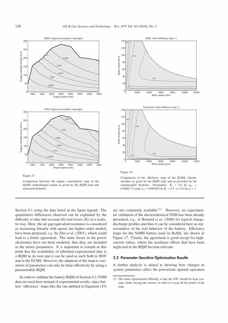
The HyHiL engine is a 2� turbocharged engine. Theengine fuel consumption map (experimental data) is shownin Figure 15 together with the BQM generated in Sec-tion 3.2, to which a new torque limit has been added to rep-resent the real engine operating range. The figure shows agood agreement between measured data and model outputs.

Similarly, the measured efficiency data of the permanent-magnet, synchronous electric machine are shown in Fig-ure 16, alongside with the map generated by the BQM of


Figure 15

Comparison between the engine consumption map of theHyHiL turbocharged engine as given by the BQM (top) andmeasured (bottom).

Figure 16

Comparison of the efficiency map of the HyHiL electricmachine as given by the BQM (top) and as provided by themanufacturer (bottom). Parameters: Rs = 0.2 Ω, ϕm =

0.88867 V·s/rad, Ls = 0.002835 H, Ri = 0.3 ·ω+0.5 Ω, p = 1.

Section 4.1 using the data listed in the figure legend. Thequantitative differences observed can be explained by thedifficulty to take into account the iron losses (Ri) in a realis-tic way. Here, the air gap equivalent resistance is consideredas increasing linearly with speed, but higher order modelshave been proposed, e.g. by Zhu et al. (2001), which couldlead to a better agreement. The static losses in the powerelectronics have not been modeled, thus they are includedin the motor parameters. It is important to remark at thispoint that the availability of tabulated experimental data isa BQM in its own and it can be used as such both in HOTand in the ECMS. However, the adaption of the map to vari-ations of parameters can only be done effectively by using aparametrable BQM.

In order to validate the battery BQM of Section 4.2, FDMdata are used here instead of experimental results, since bat-tery ‘efficiency’ maps like the one defined in Equation (43)

are not commonly available (7). However, an experimen-tal validation of the electrochemical FDM has been alreadypresented, e.g., in Bernard et al. (2008) for typical charge-discharge profiles and thus it can be considered here as rep-resentative of the real behavior of the battery. Efficiencymaps for the NiMH battery used in HyHiL are shown inFigure 17. Clearly, the agreement is good except for high-current values, where the nonlinear effects that have beenneglected in the BQM become relevant.

5.2 Parameter-Sensitive Optimization Results

A further analysis is aimed at showing how changes insystem parameters affect the powertrain optimal operation

(7) The main experimental difficulty is that the SOC should be kept con-stant while varying the current, in order to sweep all the points of themap.


calculated by HOT and that controlled by the ECMS. Inparticular, two system parameters, namely, motor power andbattery capacity, are varied with respect to the baseline caseas listed in Table 1. The results below refer to the samedrive cycle (NEDC) performed in charge-sustaining mode,that is, the battery SOC at the end of the cycle is kept closeto the initial value. Both in HOT and in the ECMS, that is aconsequence of the optimal control algorithms adopted.

TABLE 1

Baseline and modified data for the electric motor and the batteryof the HyHiL system

Case Motor power Battery capacity

1 (basel.) 45 kW 5 Ah

2 15 kW 2.5 Ah

3 22.5 kW 1.25 Ah

State of Charge (--)

State of Charge (--)

Figure 17

Comparison of the efficiency map of the HyHiL battery(NiMH) as given by the FDM (top) and the BQM (bottom).Parameters: capacity = 5 Ah, ncell = 96, voltage = 115 V.

5.2.1 Optimization with HOT

Since HOT is purely based on BQM’s to represent the sys-tem, changes in the latter directly affect the trajectories cal-culated, as shown in Figures 18, 19.

The results are plotted in terms of engine and motoroperating points in the respective efficiency maps, along theNEDC speed profile. With HOT, these points result from thedynamic minimization of the overall fuel consumption withthe major constraint of battery charge sustaining along thecycle. In this case, reducing the size of the electric motorreduces the room for recharging the battery, both usingregenerative braking and using the engine. The latter influ-ence is also visible in the engine operating points, whichexhibit a trend in moving toward lower load regions whencase 2 is applied. The use of the engine is then restricted bythe generating limits of the electric machine.

5.2.2 ECMS in Co-simulation

The online controller ECMS uses the same models as HOTto calculate the optimal control outputs. On the other hand,

Figure 18

Operating points of the engine on the NEDC with HOT for thedata cases 1 and 2, see Table 1.


Figure 19

Operating points of the motor on the NEDC with HOT for thedata cases 1 and 2, see Table 1.

the controller effects on the powertrain operation are inves-tigated by sending the control outputs to correspondingFDM’s that are run simultaneously (as described in Sect. 2).Contrarily to the previous scenario, now the driving sched-ule is not known in advance but it is estimated continuouslyfrom the action of a virtual driver that tries to follow theNEDC by adapting the current vehicle speed to the pre-scribed one acting on the pedals.

Another difference with respect to the HOT case is thatco-simulated FDM’s appropriately include the dynamics ofthe components. This is clearly shown in Figures 20, 21,where several transient operating points appear in addi-tion to a quasistatic behavior that is similar to that of Fig-ures 18, 19. The figures also show that, in such a scenarioas well, shifting from case 1 to case 2 makes the operatingpoints of the engine move towards lower load (and lowerefficiency) zones.

5.2.3 ECMS in the HyHiL Test Bench

In the HyHiL test bench control outputs of the ECMS con-troller are sent to a real engine on the one hand, and to real-

Figure 20

Operating points of the engine on the NEDC in co-simulationfor the data cases 1 and 2, see Table 1.

time FDM’s of the other components (e.g., battery, electricmotor) on the other hand. These FDM’s are then used tocontrol the bench dynamometer controller, as shown abovein Figure 4. Data are collected from real sensors on theengine and the dynamometer, and from virtual sensors in themodels. Figures 22, 23 show the operating points measuredduring a NEDC test (followed by a virtual driver as in theco-simulation scenario).

The results of the baseline case and of the case 2 (notshown) are very similar to the other scenarios (HOT and co-simulation). The figures also show the results for the case 3,where the motor power is sufficient to enable relatively high-load, high-efficiency operation of the engine (contrarily tocase 2). However, the battery size reduction leads to a muchmore aggressive SOC control, which implies several oper-ating points where the engine is strongly loaded to rechargethe battery. The result of this operation is clearly seen in


Figure 21

Operating points of the motor on the NEDC in co-simulationfor the data cases 1 and 2, see Table 1.

Figure 22 in terms of a larger dispersion of the engine oper-ating points from the best efficiency zone.

CONCLUSION

The paper has presented the concept of automated modelgeneration for hybrid powertrains. In particular, a para-metric building of backward and forward QM’s from theirrespective FDM counterparts has been proposed with thegoal of serving as a prerequisite to perform complex opti-misation and prototyping tasks with dedicated tools (HOT,HyHiL). Some examples have illustrated the concept forengines (both naturally-aspirated and turbocharged) andelectric components of HEVs. The equations derived showthe feasability of the proposed procedures, while the sim-ulation results show that such a procedure is equivalent interms of accuracy to longer simulation campaigns. More-over, the effect of changes in the components’ parameters

Figure 22

Operating points of the engine on the NEDC with HyHiL forthe data cases 1 and 3, see Table 1.

and of the consequent map adaption is clearly visible in theoptimisation and online control results.

APPENDIX

Naturally-Aspirated Engines

Forward Resolution

Given S tv and Ne, D can be deduced from Equation (1) if theflow through the throttle is sonic, since Cm depends only onthe gas properties for sonic flows. In this case, Equation (2)yields Tin and Pin is found with Equation (3). Once Pin hasbeen found, the sonic hypothesis can be checked. If it istrue, then mair and Ce are calculated with Equations (5, 4),respectively. Else, the proposed solution consists in assum-ing a value for Pin, deducing D from Equation (1), then Tin

from Equation (2), and finally calculating a new value forPin with Equation (3). If the two Pin’s are equal, a fixed


Figure 23

Operating points of the motor on the NEDC with HyHiL forthe data cases 1 and 2, see Table 1.

Figure 24

Flowchart of FQM generation for a naturally-aspirated engine.

point has been found, and mair and Ce are calculated withEquations (5, 4), respectively. This procedure is illustratedin Figure 24.

Backward Resolution

Given Ce and Ne, no equations can be solved directly. Theproposed solution is to assume a value for Pin, then calculate

Figure 25

Flowchart of BQM generation for a naturally-aspirated engine.

Figure 26

Flowchart of FQM generation for a turbocharged engine.

D and Tin from (2) and (3), and finally calculate a new Pin

with (4) and (5). If this value matches the first guess, a fixedpoint has been found, and S tv is calculated with (1). Thisprocedure is illustrated in Figure 25.

Turbocharged Engines

The resolution procedure is inspired by the same consid-erations illustrated in the previous section for naturally-aspirated engines, thus it is not further detailed. For theFQM, four algebraic loops have been identified. For theBQM, a distinction has been made between the cases inwhich the throttle valve command is active (S tv � S tv,max)and the waste gate command is active (S wg � S wg,max).The proposed methods of resolution are illustrated in Fig-ures 26-28.


Figure 27

Flowchart of BQM generation for a turbocharged engine:waste gate totally open.

REFERENCES

1 Bernard J., Sciarretta A., Touzani Y., Sauvant-Moynot V.(2008) Advances in electrochemical models for predicting thecycling performance of traction batteries: experimental studyon Ni-MH and simulation, Proc. Les Rencontres Scientifiquesde l’IFP – Advances in Hybrid Powertrains, Rueil-Malmaison,France, November 25-26, 2008.

2 Botte G.G., Subramanian V.R., White R.E. (2000) Mathemati-cal modeling of secondary lithium batteries, Electrochem. Acta45, 2595-2609.

3 Chasse A., Pognant-Gros P., Sciarretta A. (2009a) OnlineImplementation of an Optimal Supervisory Control for a Par-allel Hybrid Powertrain, SAE paper 2009–01–1868.

4 Chasse A., Hafidi G., Pognant-Gros Ph., Sciarretta, A. (2009b)Supervisory Control of Hybrid Powertrains: an ExperimentalBenchmark of Offline Optimization and Online Energy Man-agement, accepted for pubblication at the 2009 IFAC Workshopon Engine and Powertrain Control, Simulation and Modeling,Rueil-Malmaison, France, Nov. 30-Dec. 2, 2009.

5 Delagrammatikas G.J., Assanis D.N. (2004) Development ofa neural network model of an advanced, turbocharged dieselengine for use in vehicle-level optimization studies, Proc.IMEchE, Part D: J. Automobile Eng. 218, 5, 521-533.

6 Del Mastro A., Chasse A., Pognant-Gros P., Corde G., PerezF., Gallo F., Hennequet, G. (2009) Advanced Hybrid VehicleSimulation: from ‘Virtual’ to ‘HyHiL’ test bench, SAE paper2009-24-0068.

Figure 28

Flowchart of BQM generation for a turbocharged engine:throttle valve totally open.

7 Eriksson, L. (2007) Modeling and control of turbocharged Sland Dl engines, Oil Gas Sci. Technol. – Rev. IFP 62, 4, 523-538.

8 Filipi Z., Hagena J., Knafl A., Ahlawat R., Liu J., Jung D.,Assanis D., Peng H., Stein J. (2006) Engine-in-the-loop testingfor evaluating hybrid propulsion concepts and transient emis-sions – HMMWV case study, SAE paper 2006-01-0443.

9 Guzzella L., Amstutz A. (1999) CAE tools for quasi-staticmodeling and optimization of hybrid powertrains, IEEE T. Veh.Technol. 48, 6, 1762-1769.

10 Guzzella L., Onder C. (2004) Introduction to modeling andcontrol of internal combustion engine systems, Springer, BerlinHeidelberg New York.

11 Guzzella L., Sciarretta A. (2007) Vehicle propulsion systems.Introduction to modeling and optimization, 2nd ed., Springer,Berlin Heidelberg.

12 Jeanneret B., Trigui R., Malaquin B., Desbois-Renaudin M.,Badin F., Plasse C., Scordia J. (2004) Mise en oeuvre d’unecommande temps réel de transmission hybride sur banc d’essaimoteur, Proc. 2e Congrès Européen sur les AlternativesÉnergétiques dans l’Automobile, Poitiers, France, April 7-8,2004.

13 Kuhn E., Forgez C., Lagonotte P., Friedrich G. (2006) Model-ing NiMH battery using Cauer and Foster structures, J. PowerSources 158, 1490-1497.


14 Mohamed Y.A.I., Lee T.K. (2006) Adaptive self-tuning MTPAvector controller for IPMSM drive systems, IEEE T. EnergyConver. 21, 3, 636-642.

15 Moraal P., Kolmanovsky I. (1999) Turbocharger modeling forautomotive control applications, SAE paper 1999-01-0908.

16 Murgovski N., Fredriksson J., Sjöberg J. (2008) Automaticvehicle model simplification, Proc. Conf. Reglermöte, Lulea,Sweden, June 4-5, 2008.

17 Müller M., Hendricks E., Sorenson S. (1998) Mean value mod-elling of a turbocharged SI engine, SAE paper 980784.

18 Paxton B., Newman J. (1997) Modeling of nickel/metalhydride batteries, J. Electrochem. Soc. 144, 3818-3831.

19 Rousseau G., Sinoquet D., Rouchon P. (2007) ConstrainedOptimization of Energy Management for a Mild-Hybrid Vehi-cle, Oil Gas Sci. Technol. – Rev. IFP 62, 4, 623-634.

20 Rousseau G., Sinoquet D., Sciarretta A., Milhau, Y. (2008)Design optimisation and optimal control for hybrid vehicles,Proc. Int. Conf. on Engineering Optimization, Rio de Janeiro,Brazil, June 1-5, 2008.

21 Sciarretta A., Guzzella L. (2007) Control of hybrid electricvehicles. Optimal energy-management strategies, Control Syst.Mag. 27, 2, 60-70.

22 Scordia J., Desbois-Renaudin M., Trigui R., Jeanneret B.,Badin F. (2005) Global optimization of energy managementlaws in hybrid vehicles using dynamic programming, Int. J.Vehicle Des. 39, 4.

23 Serrao L., Onori S., Rizzoni G. (2009) ECMS as a realizationof Pontryagin’s minimum principle for HEV control, Proc.American Control Conference, St. Louis, MO, USA, June 10-12, 2009.

24 Sun T., Kim B.W., Lee J.H., Hong J.P. (2008) Determinationof parameters of motor simulation module employed in ADVI-SOR, IEEE T. Magn. 44, 6, 1578-1581.

25 Sundström O., Guzzella L., Soltic P. (2008) Optimal hybridiza-tion in two parallel hybrid electric vehicles using dynamic pro-gramming, Proc. 17th World IFAC Congress, Seoul, Korea,July 6-11, 2008.

26 Takano K., Nozaki K., Saito Y., Negishi A., Kato K.,Yamaguchi Y. (2000) Simulation study of electrical dynamiccharacteristics of lithium-ion battery, J. Power Sources 90, 2,214-233.

27 Urasaki N., Senjyu T., Uezato K. (2000) An accurate modelingfor permanent magnet synchronous motor drives, Proc. 15thIEEE Applied Power Electronics Conference and Exposition,New Orleans, LA, USA, February 6-10, 2000.

28 Wu B., Mohammed M., Brigham D., Elder R., White R.E.(2001) A non-isothermal model of a nickel-metal hydride cell,J. Power Sources 101, 149-157.

29 Zhang Q., White R.E. (2007) Comparison of approximate solu-tion methods for the solid phase diffusion equation in a porouselectrode model, J. Power Sources 165, 880-886.

30 Zhu Z.Q., Ng K., Howe D. (2001) Analytical Prediction ofStator Flux Density Waveforms and Iron Losses in BrushlessDC Machines, Accounting for Load Conditions, Proc. FifthInternational Conference on Electrical Machines and Systems2, 814-817.

Final manuscript received in September 2009Published online in January 2010

Copyright © 2010 Institut français du pétrolePermission to make digital or hard copies of part or all of this work for personal or classroom use is granted without fee provided that copies are not madeor distributed for profit or commercial advantage and that copies bear this notice and the full citation on the first page. Copyrights for components of thiswork owned by others than IFP must be honored. Abstracting with credit is permitted. To copy otherwise, to republish, to post on servers, or to redistributeto lists, requires prior specific permission and/or a fee: Request permission from Documentation, Institut français du pétrole, fax. +33 1 47 52 70 78, or [email protected].

automated model generation for hybrid vehicles

Documents