ARTICLE IN PRESS

0098-3004/$ - se

doi:10.1016/j.ca

�Correspondfax: +1281 486

E-mail addr

Computers & Geosciences ] (]]]]) ]]]–]]]

www.elsevier.com/locate/cageo

Automated classification of landforms on Mars

B.D. Buea, T.F. Stepinskib,�

aDepartment of Computer Science, Purdue University, 250 N. University St., West Lafayette, IN 47907, USAbLunar and Planetary Institute, 3600 Bay Area Blvd., Houston, TX 77058, USA

Received 25 February 2005; received in revised form 7 September 2005; accepted 7 September 2005

Abstract

We propose a numerical method for classification and characterization of landforms on Mars. The method provides an

alternative to manual geomorphic mapping of the Martian surface. Digital elevation data is used to calculate several

topographic attributes for each pixel in a landscape. Unsupervised classification, based on the self-organizing map

technique, divides all pixels into mutually exclusive and exhaustive landform classes on the basis of similarity between

attribute vectors. The results are displayed as a thematic map of landforms and statistics of attributes are used to assign

semantic meaning to the classes. This method is used to produce a geomorphic map of the Terra Cimmeria region on Mars.

We assess the quality of the automated classification and discuss differences between results of automated and manual

mappings. Potential applications of our method, including crater counting, landscape feature search, and large scale

quantitative comparisons of Martian surface morphology, are identified and evaluated.

r 2005 Elsevier Ltd. All rights reserved.

Keywords: Landform classification; Self-organizing maps; Digital topography models; Automated techniques; Mars

1. Introduction

Mapping of landforms on planetary surfaces istraditionally done via photogeologic interpretationof images (Wilhelms, 1990; Tanaka, 1994). Thismanual method is slow and labor intensive. Thehigh ‘‘cost’’ of standard planetary mapping severelylimits the number of sites that can be studied indetail. For planet Mars, the availability of digitalelevation data suggests applying automated land-form mapping techniques to speed up the processand reduce costs. In the terrestrial context, auto-mated methods have previously been developed to

e front matter r 2005 Elsevier Ltd. All rights reserved

geo.2005.09.004

ing author. Tel.: +1281 486 2170;

2162.

ess: tom@lpi.usra.edu (T.F. Stepinski).

identify various individual terrain features (such asvalley heads, streams, ridges, and watersheds) fromdigital elevation models (DEMs). These methodswere subsequently applied to Martian terrain(Stepinski and Collier, 2004). However, to alleviatethe slowness of manual mapping, a general auto-mated landform classifier that completely subdi-vides a landscape into constituent landforms isneeded. Such classifiers were developed in variousterrestrial contexts (Guzzetti and Reichenbach,1994; Dymond et al., 1995; Irvin et al., 1997;Burrough et al., 2000; Hosokawa and Hoshi, 2001),but they are too specific to their respective domainsof application to be adapted for classification ofMartian landscapes.

In this paper we present an automated methodfor classification of landforms on Mars. The overall

.

ARTICLE IN PRESSB.D. Bue, T.F. Stepinski / Computers & Geosciences ] (]]]]) ]]]–]]]2

design of the method is general enough to beapplicable to any surface including terrestrial land-scapes; however, topographic attributes have beenchosen to optimize identification of landformscommon on Mars but rare on Earth. The methoduses the concept of a digital topography model(DTM) developed by Stepinski and Vilalta (2005).The DTM is an organization of a site’s topographicdata into a three-dimensional (3-D) array consistingof several two-dimensional (2-D) layers with eachlayer holding a different topographic attributeorganized in a spatial grid common to all layers.By construction, the DTM is somewhat analogousto the concept of a multispectral image, but itpertains to topographic rather than imagery data.The DTM can also be viewed as an extension of thefamiliar notion of the DEM, with the first layerstoring elevation values, and subsequent layersstoring additional topographic information.

A pixel in the DTM carries a vector oftopographic attributes. It is expected that pixelsconstituting a particular landform carry similarattribute vectors. Attribute vectors are similar if theEuclidean distance between them is small. Classifi-cation of landforms in a given site is achieved byapplying a clustering algorithm over all attributevectors in this site. The output of the clusteringalgorithm is a set of K mutually exclusive andexhaustive classes. Each class contains a set ofattribute vectors similar to each other. The set ofpixels affiliated with vectors belonging to a specificclass constitutes a particular landform. For such aclassification to be practical, the clustering algo-rithm must be efficient and the resultant landformsmust show high spatial coherence. In the context ofremote sensing applications, the most widely usedclustering schemes are k-means and ISODATAalgorithms (Jain and Dubes, 1988). These methodsare not particularly efficient and yield classes that,sometimes lack a high degree of spatial integrity. Inan attempt to overcome these shortcomings Ste-pinski and Vilalta (2005) classified the DTM using aprobabilistic clustering algorithm working under theBayesian framework. Spatially coherent landformswere identified, but the algorithm proved to beinefficient and thus unable to classify sites ofsignificant size on Mars. In the present method,the clustering efficiency is significantly improved byreplacing the probabilistic clustering algorithm by atwo-level procedure similar to the one described byVesanto and Alhoniemi (2000) consisting of a self-organizing map (SOM) (Kohonen, 1995) and the

Ward hierarchical clustering method (Ward, 1963).Note that we are using an unsupervised clusteringalgorithm in which no specific landforms areprescribed beforehand, instead the set of landforms‘‘emerges’’ from the data. Such a design maximizesthe level of automation and allows for the potentialdiscovery of novel landforms that could be over-looked in manual mapping.

2. Topographic attributes for Martian surfaces

The choice of topographic attributes depends onthe goal of classification. For example, the study ofIrvin et al. (1997), motivated by the relation betweenlandforms and soil properties, used the followingattributes: elevation, slope, curvature, wetnessindex, and incident solar radiation. We anticipatethat on Mars, an automated classification would beused mostly to study highly cratered ancient high-lands. Topographic basins, of which craters are themost abundant example, are an important compo-nent of the highland landscape. Our choice ofattributes reflects the need to identify and char-acterize these basins.

To address the issue of the topographic basins, weconsider, in addition to the original elevation field,an elevation field artificially modified by using a so-called ‘‘flooding’’ algorithm (O’Callaghan andMark, 1984). The flooding algorithm identifies allenclosed depressions in the original elevation fieldand raises their elevations to the level of the lowestpour point around their edges. The differencebetween the flooded and original elevation fields,hereafter referred to as the ‘‘flood’’, has non-zerovalues only for pixels located inside topographicbasins. The six attributes used in our method arederived from original and flooded elevation fields,they are: elevation, flood, slope, flooded slope,contributing area, and flooded contributing area.The flooded slope and flooded contributing area arecalculated using the flooded elevation field. Theseattributes are calculated for every pixel and storedin subsequent layers of the DTM. The standardmethod to infer the terrain’s drainage from theDEM (Tarboton et al., 1989) is to draw a linkbetween every pixel and one of its nearest neighborsfollowing the steepest descent direction. Thisprocedure organizes all pixels into a number ofspanning tree structures. The contributing areaof a given pixel is the area of all pixels locatedabove it in the tree structure. The magnitude of the

ARTICLE IN PRESSB.D. Bue, T.F. Stepinski / Computers & Geosciences ] (]]]]) ]]]–]]] 3

contributing area variable is used to identify ridgesand channels.

3. Methods

The implementation of our classifier was designedto take advantage of software packages that are inthe public domain. The schematic view of the entireprocess is shown on Fig. 1. There are sevenconsecutive steps in the process, from data acquisi-tion to semantic annotation of all pixels in theDTM.

Martian topography data gathered by the MarsOrbiter Laser Altimeter (MOLA) instrument (Zuberet al., 1992) was used to construct (Smith et al.,2003) the Mission Experiment Gridded DataRecords (MEGDR), which are global topographicmaps of Mars with resolution of 128 pixels/degree.This large dataset is organized into 16 ‘‘tiles’’covering different latitudes. In the first step (A) asimple script constructs a DEM for a site of interest(that may be located across multiple tiles). Thisscript also reprojects the MEGDR data fromspherical to local cartesian coordinates.

The software suite TARDEM (Tarboton et al.,1989), originally developed for studies of terrestrialbasins, calculates the six topographic attributes. ADEM acquired in step (A) requires some preproces-sing before it can be used as an input forTARDEM. Some spanning tree structures repre-senting drainage are cut short by the DEMs edgewhich discards portions of these trees outside theDEM. The contributing area cannot be accuratelycalculated for pixels belonging to these trees becauseof the unknown contribution from the outside of theDEM. This problem is referred to as the ‘‘edgecontamination.’’ In the first preprocessing step (B1)the DEM is ‘‘decontaminated’’ by lowering theelevation values of the pixels located at the edges ofthe DEM to the lowest recorded elevation value inthe entire DEM, thus isolating the site from outsidecontributions. In the second preprocessing step (B2)

MEGDR (A)

Calculating contentsof layers in the DTM(C)

INPUT TARDEMpreprocessing

TARDEMpo

Calculating Topographic Attributes

OutDistchaNor

Elimedg

DEMdecontamination (B1)

Datareformatting (B2)

Fig. 1. A schematic view of computational process lea

the header required by the TARDEM is prependedto the decontaminated DEM. In the third step (C)the TARDEM algorithm takes a decontaminatedDEM as input and calculates the six layers of theDTM.

The DTM calculated by TARDEM requiressome postprocessing in order to make it ready forclustering. First, the pixels located at a double edgeof the DTM are eliminated (D1). This reduces theplanar dimensions of the DTM from N �M toðN � 4Þ � ðM � 4Þ. The eliminated pixels carryspurious values of the attributes and retaining themwould lead to ‘‘discovery’’ of landforms that lackphysical meaning. Second, the MEGDR data isgenerally of high quality, but occasional pixelscontain spurious elevation values leading to ex-istence of outliers in the DTM. These outliers aredetected and eliminated (D2). The distributions(probability distribution functions, hereafter re-ferred to as pdf) of all topographic attributes arereviewed (D3) to check their character. Someattributes, such as slope and contributing area havepower law pdfs. This complicates the issue of layernormalization (see below). In cases where this is aproblem we replace the original attribute by itscommon logarithm. The attributes stored in differ-ent layers of the DTM have different physicalmeanings and different ranges of values. In the finalTARDEM postprocessing step (D4), each attributeis normalized so that its values are in the rangeð0; 1Þ. This normalization causes all variables tocontribute equally to the ‘‘distance’’ betweendifferent pixels.

Two steps (E and F) perform the actualclassification of attribute vectors. Note thatalthough the DTM has a spatial structure, thisspatial information is not used in the process ofclassification. Instead, pixels are assigned to land-form classes exclusively on the basis of the values oftheir topographic attributes.

The first step (E) of the classification methodcreates a self-organizing map (SOM). The SOM

CalculatingSOM (E)

Wardclustering (F) thematic map (G)

TARDEMstprocessing

SOM_PAK R OUTPUT

Classification

liers (D2)ributionracter (D3)malization (D4)

inatinges (D1)

ding to an automated classification of landforms.

ARTICLE IN PRESSB.D. Bue, T.F. Stepinski / Computers & Geosciences ] (]]]]) ]]]–]]]4

(Kohonen, 1995) is a neural network technique thatgroups similar vectors into nearby points on a 2-Dgrid composed of nodes. Through an unsupervised,iterative procedure, the set of attribute vectors (alarge number, of the order of 107 in our applica-tions) is mapped onto the grid’s nodes (a smallnumber, of the order of 102–103) in such a way thatsimilar attribute vectors are associated with neigh-boring nodes. Because the number of nodes is muchsmaller than the number of vectors, many vectorsare mapped onto a single node. This mapping servesas an interim clustering of attribute vectors into theSOM’s nodes. The SOM for the DTM is createdusing the SOM_PAK package (Kohonen et al.,1996). We use a 30� 30 rectangular SOM grid witha Gaussian neighborhood. Experimentation withlarger grid sizes did not result in noticeably higherquality clusterings.

The bundle of attribute vectors associated with agiven node can be typified by a single representativevector called a codebook vector in the SOM_PAK.The final clustering (F) of attribute vectors isachieved by segmentation of the SOM grid ofcodebook vectors into an assigned number ofclusters, K. Each cluster groups similar codebookvectors, and thus, it groups all attribute vectorsassociated with them. The number of final clusters isa free parameter, we have experimented withK ¼ 12, 15, 20, and 40 clusters. This final clusteringis performed using the Ward’s minimum variancegrouping algorithm (Ward, 1963). This agglomera-tive, hierarchical clustering method partitions data(codebook vectors) in a manner which minimizesthe ‘‘information loss’’ associated with each group-ing. At each step in the analysis, the union of everypossible cluster pair is considered, and the twoclusters whose fusion results in the minimum loss ofinformation are combined. Ward clustering isperformed using the statistical computing environ-ment R (Ripley, 2001).

The final result of our classification procedure is athematic map of topography (G). Formally, such amap is a matrix of the same dimension as the planardimension of the DTM (ðN � 4Þ � ðM � 4Þ). Eachpixel in the thematic map is assigned a label of acluster to which a corresponding attribute vector inthe DTM belongs. The classification can bevisualized by assigning different colors to differentclusters. The initial cluster labels are just numeralswithout any meaning. Reviewing statistical proper-ties of topographic attributes in each cluster andstudying spatial relations between different clusters

allows us to replace numerical labels with semanticlabels pertaining to landform classes that theclusters represent.

4. Classification of landforms in Terra Cimmeria,

Mars

To demonstrate the capabilities of our method,we have classified landforms in the Terra Cimmeriaregion of Mars. This large ð4106 km2

Þ site (approx-imate coordinate bounds are 1251E, 1351E, 301S,and 01N) is located mostly in the ancient Noachianhighlands, but a hemispheric dichotomy boundarypasses through its NE corner. It was previouslystudied thoroughly by Irwin and Howard (2002).The size of MEGDR-derived DEM is N ¼ 3828and M ¼ 1391. After performing the postprocessingsteps described in the previous section, the DTMhas 3824� 1387 ¼ 5; 303; 888 pixels which areclassified into K ¼ 20 landform classes. All attri-butes are used directly; we have chosen not totransform any attributes.

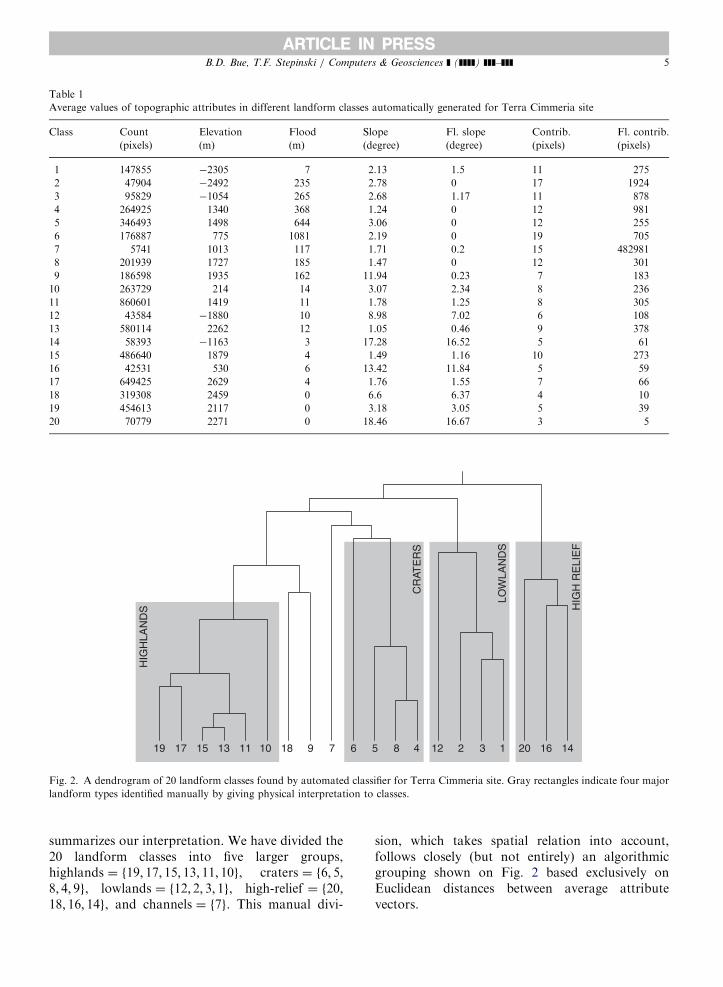
Table 1 lists the values of topographic attributesaveraged over pixels constituting each landformclass. The first column of Table 1 contains classnumerical labels and the second column containsthe number of pixels in a class. The remaining sixcolumns show average values of elevation, flood,slope, flooded slope, contributing area, and floodedarea, respectively. Those average values are usedto construct a dendrogram of landform classesshown on Fig. 2. A dendrogram summarizessimilarity relations between different classes.Similar classes are joined by links whose positionsindicate the level of similarity between theclasses. For example, the diagram on Fig. 2 showsthat out of all possible pairs, the classes 13 and 15are the most similar to each other. It also indicatesthat all 20 classes could be naturally divided into5 larger groups, A ¼ f19; 17; 15; 13; 11; 10; 18; 9g,B ¼ f7g, C ¼ f6; 5; 8; 4g, D ¼ f12; 2; 3; 1g, andE ¼ f20; 16; 14g. These groups correspond to majortypes of landforms.

Fig. 3 shows a side-by-side comparison of theTerra Cimmeria site topography and the thematicmap constructed on the basis of classification oflandforms. Different colors indicate pixel classmembership. Physical interpretation was given toeach class on the basis of reviewing statisticalproperties of topographic attributes of pixels con-stituting that class and studying spatial relationsbetween different classes. The legend on Fig. 3

ARTICLE IN PRESS

HIG

HLA

ND

S

CR

ATE

RS

LOW

LAN

DS

HIG

H R

ELI

EF

19 17 15 13 11 10 18 9 7 6 5 8 4 12 2 3 1 20 16 14

Fig. 2. A dendrogram of 20 landform classes found by automated classifier for Terra Cimmeria site. Gray rectangles indicate four major

landform types identified manually by giving physical interpretation to classes.

Table 1

Average values of topographic attributes in different landform classes automatically generated for Terra Cimmeria site

Class Count Elevation Flood Slope Fl. slope Contrib. Fl. contrib.

(pixels) (m) (m) (degree) (degree) (pixels) (pixels)

1 147855 �2305 7 2.13 1.5 11 275

2 47904 �2492 235 2.78 0 17 1924

3 95829 �1054 265 2.68 1.17 11 878

4 264925 1340 368 1.24 0 12 981

5 346493 1498 644 3.06 0 12 255

6 176887 775 1081 2.19 0 19 705

7 5741 1013 117 1.71 0.2 15 482981

8 201939 1727 185 1.47 0 12 301

9 186598 1935 162 11.94 0.23 7 183

10 263729 214 14 3.07 2.34 8 236

11 860601 1419 11 1.78 1.25 8 305

12 43584 �1880 10 8.98 7.02 6 108

13 580114 2262 12 1.05 0.46 9 378

14 58393 �1163 3 17.28 16.52 5 61

15 486640 1879 4 1.49 1.16 10 273

16 42531 530 6 13.42 11.84 5 59

17 649425 2629 4 1.76 1.55 7 66

18 319308 2459 0 6.6 6.37 4 10

19 454613 2117 0 3.18 3.05 5 39

20 70779 2271 0 18.46 16.67 3 5

B.D. Bue, T.F. Stepinski / Computers & Geosciences ] (]]]]) ]]]–]]] 5

summarizes our interpretation. We have divided the20 landform classes into five larger groups,highlands ¼ f19; 17; 15; 13; 11; 10g, craters ¼ f6; 5;8; 4; 9g, lowlands ¼ f12; 2; 3; 1g, high-relief ¼ f20;18; 16; 14g, and channels ¼ f7g. This manual divi-

sion, which takes spatial relation into account,follows closely (but not entirely) an algorithmicgrouping shown on Fig. 2 based exclusively onEuclidean distances between average attributevectors.

ARTICLE IN PRESS

Fig. 3. A shaded relief of Terra Cimmeria region on Mars (left). Thematic map of automatically identified landforms for Terra Cimmeria

region (middle). Legend ascribing physical meaning to landform classes (left). Numbers in brackets represent number of pixels in a class.

Symbol in upper-left corner of a color-coding rectangle is class numerical label.

B.D. Bue, T.F. Stepinski / Computers & Geosciences ] (]]]]) ]]]–]]]6

The pdfs of all topographic attributes for pixels inclasses 17, 15, 13, 11, and 10 are very similar, exceptfor the pdfs of elevations that divide the elevationrange into the five non-overlapping regions, fromthe highest (class 17) to the lowest (class 10). Thepixels in these classes have small values of the slopeand flood attributes. Spatially, the pixels in these 5

classes are located in the highlands, above theescarpment, filling the space between craters. Theclass 19 is similar to classes 15 and 13, but has ahigher average slope value. Spatially, most pixelsbelonging to class 19 form a transition terrainbetween landforms labeled as class 13 and class 15.Common values of attributes in these six classes

ARTICLE IN PRESSB.D. Bue, T.F. Stepinski / Computers & Geosciences ] (]]]]) ]]]–]]] 7

indicate a common landform type, an interpretationconfirmed by spatial distribution of pixels in theseclasses. Together, they form a inter-crater plateaulocated in the highlands, and we refer to themcollectively as ‘‘highlands.’’ The major discriminantbetween highland classes is the value of elevation.62.12% of pixels in the Terra Cimmeria site areclassified as highlands.

The pdfs of topographic attributes for pixels inclasses 6, 5, 9, 4, and 8 are similar, except for pdfs ofthe flood that divide the flood range into 5 distinctregions, from the largest flood (class 6) to thesmallest flood (class 9). The pixels in these classeshave small values of the slope except for pixels inclass 9 that have high slopes. These classes areidentified as the terrain inside craters and otherbasins. We bundle them into a larger group whichwe call ‘‘craters.’’ 22.19% of pixels in the TerraCimmeria site are classified as craters. The majordiscriminant between crater classes is the value ofthe flood.

Pixels in classes 18 and 20 are located athighlands at high elevations, whereas pixels inclasses 16 and 14 are located at lower elevation inthe vicinity of the escarpment. The commoncharacteristic of all pixels in these four classes isthe relatively high value of the slope. We bundlethese four classes into a larger group, that we call‘‘high relief’’ terrain. The 9.26% of pixels in theTerra Cimmeria site are classified as high relief.

The common characteristic of pixels in classes1; 2; 3, and 12 is a very low elevations. Spatially,they are all located below the escarpment, so webundle them together into a larger group referred toas ‘‘lowlands.’’ 6.32% of pixels in the TerraCimmeria site are classified as lowlands. Finally,pixels in class 7 are characterized by a large value offlooded contributed area. These pixels are the partof the landscape that constitutes a major drainagesystem, we refer to this class as ‘‘channels.’’ Thereare only 5741 pixels in this class.

5. Review of Terra Cimmeria results

The topographic map on Fig. 3 depicts a complexlandscape. In particular, there exists a rich variety ofdifferent kinds of craters. In addition to pristinecraters, there are craters superimposed on othercraters, eroded, or otherwise transformed by cir-cumstances particular to a given location. Becauseof this diversity, the basic premise of our method(that landforms consist of pixels with similar

attribute vectors), could be frequently violated.However, a visual comparison of topography withthe thematic map of landforms on Fig. 3 revealsthat our classification is, overall, in good agreementwith what one would expect. Nevertheless, there areplaces in the site, where, due to local circumstances,the automatic classifier misclassifies pixels. In theremainder of this section we discuss some of themost common misclassifications.

Most of the misclassifications are for the pixelslocated inside the craters. On occasion, a misclassi-fication occurs because a similarity measure betweenattribute vectors does not correspond to actualsimilarity of landforms. An example of such amisclassification is the floor of the large craterlocated at (1331E, 6.51S) near the dichotomyboundary. The crater is flooded, but its floor islocated at such a low elevation that the majority ofits pixels are classified as class 3 instead of class 6. Inmost cases, the misclassifications are an unavoid-able side effect of the method used for flaggingpixels inside the craters. Because craters aretopographical basins, the pixels inside them arerecognized by a large value of the flood attribute.However, the flooding algorithm ‘‘fills’’ the basinonly to the level of the lowest pour point around itsedges. A crater with undisturbed walls is flooded tothe rim and its inside pixels are classified correctly.A crater with a breached wall is only partiallyflooded and its inside pixels are misclassified. Thedegree of misclassification depends on the severityof the breach. The craters trimmed by the edge ofthe DTM are not flooded at all and their pixels areseverely misclassified. For this reason the bound-aries of a site should be chosen in such a way as tominimize these trimmed craters.

In order to discuss this issue in greater detail, wehave selected five craters for closer examination.They are labeled as A (125.51E, 21.71S), B (128.81E,3.51S), C (130.31E, 4.51S), D (128.51E, 8.51S), and E(134.71E, 9.51S). Fig. 4 shows close-up views ofcraters A, B, and C. The upper panels displaytopography by showing topographic contourssuperimposed on a shaded relief. The lower panelsshow the same topographic contours superimposedon a thematic map of landforms.

The close-up view reveals that the walls of craterA are breached at the �7 o’clock direction byanother crater. This results in an incomplete flood-ing of crater A. The pour point level is such thatmost of the pixels on the crater floor are locatedbelow it and are assigned to class 4. Some floor

ARTICLE IN PRESS

Fig. 4. Close-up views of craters A, B, and C. Upper panels show topographic contours superimposed on a shaded relief. Lower panels

show same topographic contours superimposed on a thematic map of landforms. Numbers indicate numerical labels of landform classes.

B.D. Bue, T.F. Stepinski / Computers & Geosciences ] (]]]]) ]]]–]]]8

pixels are above the pour point level and getassigned to classes 11 or 19. In addition, pixelslocated on the walls get assigned to classes 18 and 20instead of to class 9. The small crater causing thebreach is heavily eroded and does not constitute abasin, its interior gets assigned to class 11. A smallcrater located at the �1 o’clock direction abovecrater A constitutes a very shallow basin. Its wallsare assigned correctly as class 9, but its floor pixelsare assigned to class 17 because of high elevationand minimal flood.

A close-up view of crater B shows a breach in itsrim at the �12 o’clock direction. This minimalbreach results in high pour point level. Conse-quently, the classification of most of the interior of

this crater remains unaffected by the breach. Incontrast, crater C is heavily eroded and its shallowwalls are breached at the �2 o’clock direction. Thepour point level is very low, resulting in minimalflooding. As a result, most of the pixels in theinterior of this crater are assigned to highlandclasses 10 and 11. Only a few deeper spots areclassified as shallow crater floors (class 4).

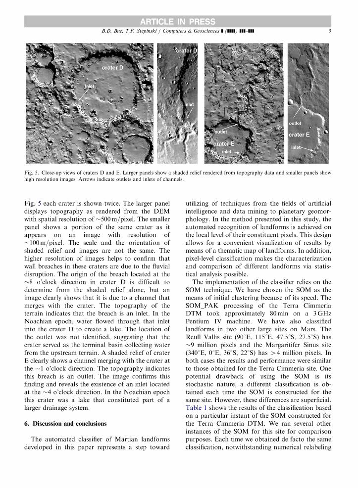
In most cases, the crater walls are breached byerosion or superposition of other craters, but somecraters are breached by merging channels. Thesecraters are of high interest because, in the Noachianepoch, they were lakes constituting part of adrainage system. Craters D and E, shown onFig. 5 are the two examples of such features. On

ARTICLE IN PRESS

Fig. 5. Close-up views of craters D and E. Larger panels show a shaded relief rendered from topography data and smaller panels show

high resolution images. Arrows indicate outlets and inlets of channels.

B.D. Bue, T.F. Stepinski / Computers & Geosciences ] (]]]]) ]]]–]]] 9

Fig. 5 each crater is shown twice. The larger paneldisplays topography as rendered from the DEMwith spatial resolution of �500m=pixel. The smallerpanel shows a portion of the same crater as itappears on an image with resolution of�100m=pixel. The scale and the orientation ofshaded relief and images are not the same. Thehigher resolution of images helps to confirm thatwall breaches in these craters are due to the fluvialdisruption. The origin of the breach located at the�8 o’clock direction in crater D is difficult todetermine from the shaded relief alone, but animage clearly shows that it is due to a channel thatmerges with the crater. The topography of theterrain indicates that the breach is an inlet. In theNoachian epoch, water flowed through that inletinto the crater D to create a lake. The location ofthe outlet was not identified, suggesting that thecrater served as the terminal basin collecting waterfrom the upstream terrain. A shaded relief of craterE clearly shows a channel merging with the crater atthe �1 o’clock direction. The topography indicatesthis breach is an outlet. The image confirms thisfinding and reveals the existence of an inlet locatedat the �4 o’clock direction. In the Noachian epochthis crater was a lake that constituted part of alarger drainage system.

6. Discussion and conclusions

The automated classifier of Martian landformsdeveloped in this paper represents a step toward

utilizing of techniques from the fields of artificialintelligence and data mining to planetary geomor-phology. In the method presented in this study, theautomated recognition of landforms is achieved onthe local level of their constituent pixels. This designallows for a convenient visualization of results bymeans of a thematic map of landforms. In addition,pixel-level classification makes the characterizationand comparison of different landforms via statis-tical analysis possible.

The implementation of the classifier relies on theSOM technique. We have chosen the SOM as themeans of initial clustering because of its speed. TheSOM_PAK processing of the Terra CimmeriaDTM took approximately 80min on a 3GHzPentium IV machine. We have also classifiedlandforms in two other large sites on Mars. TheReull Vallis site (901E, 1151E, 47.51S, 27.51S) has�9 million pixels and the Margaritifer Sinus site(3401E, 01E, 361S, 221S) has 44 million pixels. Inboth cases the results and performance were similarto those obtained for the Terra Cimmeria site. Onepotential drawback of using the SOM is itsstochastic nature, a different classification is ob-tained each time the SOM is constructed for thesame site. However, these differences are superficial.Table 1 shows the results of the classification basedon a particular instant of the SOM constructed forthe Terra Cimmeria DTM. We ran several otherinstances of the SOM for this site for comparisonpurposes. Each time we obtained de facto the sameclassification, notwithstanding numerical relabeling

ARTICLE IN PRESSB.D. Bue, T.F. Stepinski / Computers & Geosciences ] (]]]]) ]]]–]]]10

of classes as well as small changes in pixel countsand average values of attributes.

The thematic map of landforms in Terra Cim-meria site is a type of a geomorphic map. Thisinvites a comparison to a manually constructedgeomorphic map of the same region shown in Irwinand Howard (2002). The comparison reveals aninteresting contrast between automated and manualmappings. There is no standard of what constitutesa geomorphic map. Irwin and Howard wereinterested in drainage basin evolution in TerraCimmeria, and thus emphasized impact craters,channel networks, drainage basins divides, anddepositional basins in their manual mapping. Eachlandform class on their map has a narrowly definedsemantic meaning because it was deliberately chosenbefore the actual mapping. In contrast, the auto-mated mapping results in a less focused, more‘‘general purpose’’ map with broadly definedsemantic meanings of landform classes. This reflectsthe unsupervised character of the classifier; nolandforms are defined beforehand and their mean-

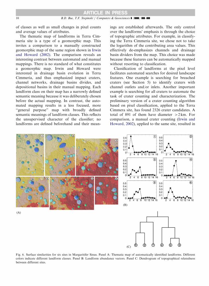
Fig. 6. Surface similarities for six sites in Margaritifer Sinus. Panel A

colors indicate different landform classes. Panel B: Landform abunda

between different sites.

ings are established afterwards. The only controlover the landforms’ emphasis is through the choiceof topographic attributes. For example, in classify-ing the Terra Cimmeria site, we chose not to takethe logarithm of the contributing area values. Thiseffectively de-emphasizes channels and drainagebasin dividers from the map. This choice was madebecause these features can be automatically mappedwithout resorting to classification.

Classification of landforms at the pixel levelfacilitates automated searches for desired landscapefeatures. One example is searching for breachedcraters (see Section 5) to identify craters withchannel outlets and/or inlets. Another importantexample is searching for all craters to automate thetask of crater counting and characterization. Thepreliminary version of a crater counting algorithmbased on pixel classification, applied to the TerraCimmera site, has found 2326 crater candidates. Atotal of 891 of them have diameter 42 km. Forcomparison, a manual crater counting (Irwin andHoward, 2002), applied to the same site, resulted in

: Thematic map of automatically identified landforms. Different

nce vectors. Panel C: Dendrogram of topographical relatedness

ARTICLE IN PRESSB.D. Bue, T.F. Stepinski / Computers & Geosciences ] (]]]]) ]]]–]]] 11

890 craters with diameter 42 km. Further work isneeded to assure that all counted features are indeedcraters and that all craters are counted.

Finally, the automated classifier enables a quan-titative determination of topographic similaritiesbetween different sites. Fig. 6 (panel A) shows athematic map of landforms for six adjacent sites inthe Margaritifer Sinus region of Mars. The siteswere processed separately but classified togetherinto 15 landform classes. For each site, we calculatea 15-dimensional ‘‘landform abundance’’ vectorconsisting of fractions of pixels in each landformclass. Fig. 6 (panel B) depicts landform abundancevectors for all six sites. These six vectors areclustered using the Ward grouping method (seeSection 3) and their similarity relations are sum-marized using a dendrogram (panel C on Fig. 6).The dendrogram displays a quantitative degree oftopographical relatedness between different sites inthe Margaritifer Sinus region. These computedsimilarity relations are in an agreement with avisual impression of topographic similarity betweenthe different sites. A similar calculation, but on themuch larger scale (a large number of sites), wouldenable a quantitative comparative study of Martiansurface morphology.

Acknowledgements

This research was supported by NSF under grantIIS-0430208. A portion of this research wasconducted at the Lunar and Planetary Institute,which is operated by the USRA under contractCAN-NCC5-679 with NASA. This is LPI Con-tribution No. 1236.

References

Burrough, P.A., van Gaans, P.F.M., MacMillan, R.A., 2000.

High-resolution landform classification using fuzzy k-means.

Fuzzy Sets and Systems 113, 37–52.

Dymond, J.R., De Rose, R.C., Harmsworth, G.R., 1995.

Automated mapping of land components from digital

elevation data. Earth Surface Processes and Landforms 20,

131–137.

Guzzetti, F., Reichenbach, P., 1994. Towards a definition of

topographic divisions for Italy. Geomorphology 11, 57–74.

Hosokawa, M., Hoshi, T., 2001. Landform classification method

using self-organizing map and its application to earthquake

damage evaluation. IEEE 2001 Geoscience and Remote

Sensing Symposium, pp. 1684–1686.

Irvin, B.J., Ventura, S.J., Slater, B.K., 1997. Fuzzy and

isodata classification of landform elements from digital

terrain data in Pleasant Valley, Wisconsin. Geoderma 77,

137–154.

Irwin III, R.P., Howard, A.D., 2002. Drainage basin evolution in

Noachian Terra Cimmeria Mars. Journal of Geophysical

Research 107 E7, 10-1–10-23.

Jain, A.K., Dubes, R.C., 1988. Algorithms for Clustering Data.

Prentice-Hall, Englewood Cliffs, NJ.

Kohonen, T., 1995. Self-organizing Maps. Springer, Berlin.

Kohonen, T., Hynninen, J., Kangas, J., Laaksonen, J., 1996.

SOM_PAK: the self-organizing map program package.

Technical Report A31, Helsinki University of Technology,

Laboratory of Computer and Information Science, FIN-

02150 Espoo, Finland.

O’Callaghan, J.F., Mark, D.M., 1984. The extraction of drainage

networks from digital elevation data. Computer Vision,

Graphics and Image processing 28, 328–344.

Ripley, B.D., 2001. The R project in statistical computing,

MSOR connections. The Newsletter of the LTSN Mathe-

matics, Statistics & OR Network 1 (1), 23–25.

Smith, D., Neumann, G., Arvidson, R.E., Guinness, E.A.,

Slavney, S., 2003. Mars Global Surveyor laser altimeter

mission experiment gridded data record. NASA Planetary

Data System, MGS-M-MOLA-5-MEGDR-L3-V1.0.

Stepinski, T.F., Collier, M.L., 2004. Extraction of Martian valley

networks from digital topography. Journal of Geophysical

Research 109, E11005.

Stepinski, T.F., Vilalta, R., 2005. Digital topography models for

Martian surfaces. IEEE Geoscience and Remote Sensing

Letters 2 (3), 260–264.

Tanaka, K.L., 1994. The Venus Geologic Mappers’

Handbook, US Geological Survey Open File Report No.

99-438.

Tarboton, D.G., Bras, R.L., Rodriguez-Iturbe, I., 1989. The

analysis of river basins and channel networks using digital

terrain data. Technical Report No. 326, Ralf M. Parsons

Laboratory, MIT, Cambridge.

Vesanto, J., Alhoniemi, E., 2000. Clustering of the self-organizing

map. IEEE Transactions on Neural Networks 11 (3),

586–600.

Ward Jr., J.H., 1963. Hierarchical grouping to optimize an

objective function. Journal of the American Statistical

Association 58 (301), 236–244.

Wilhelms, D.E., 1990. Geologic Mapping. In: Greeley, R.,

Batson, R. (Eds.), Planetary Mapping. Cambridge University

Press, Cambridge, UK, pp. 209–260.

Zuber, M.T., Smith, D.E., Solomon, S.C., Muhleman, D.O.,

Head, J.W., Garvin, J.B., Abshire, J.B., Bufton, J.L., 1992.

The mars observer laser altimeter investigation. Journal of

Geophysical Research 97 (E5), 7781–7797.