autocad 2006 2 d and 3d design
DESCRIPTION
autocadTRANSCRIPT


Introduction to AutoCAD 2006

This Page is Intentionally Left Blank

Introduction to AutoCAD 2006 2D and 3D Design
Alf Yarwood
AMSTERDAM • BOSTON • HEIDELBERG • LONDONNEW YORK • OXFORD • PARIS • SAN DIEGO
SAN FRANCISCO • SINGAPORE • SYDNEY • TOKYO
Newnes is an imprint of Elsevier

Working together to grow libraries in developing countries
www.elsevier.com | www.bookaid.org | www.sabre.org
Newnes is an imprint of ElsevierLinacre House, Jordan Hill, Oxford OX2 8DP30 Corporate Drive, Burlington, MA 01803
First published 2006
Copyright © 2006, Alf Yarwood. All rights reserved
The right of Alf Yarwood to be identified as the author of this work has been asserted in accordance with the Copyright, Designs and Patents Act 1988
No part of this publication may be reproduced in any material form (including photocopying or storing in any medium by electronic means and whether or not transiently or incidentally to some other use of this publication) without the written permission of the copyright holder except in accordance with the provisions of the Copyright, Designs and Patents Act 1988 or under the terms of a licence issued by the Copyright Licensing Agency Ltd, 90 Tottenham Court Road, London,England W1T 4LP. Applications for the copyright holder’s written permission to reproduce any part of this publication should be addressed to the publisher
Permissions may be sought directly from Elsevier’s Science and Technology Rights Department in Oxford, UK: phone: (�44) (0) 1865 843830; fax: (�44) (0) 1865 853333; e-mail: [email protected]. You may also complete your request on-line via the Elsevier homepage (http://www.elsevier.com), by selecting ‘Customer Support’and then ‘Obtaining Permissions’
British Library Cataloguing in Publication DataA catalogue record for this book is available from the British Library
Library of Congress Cataloguing in Publication DataA catalogue record for this book is available from the Library of Congress
ISBN-13: 978–0–7506–6876–7ISBN-10: 0–7506–6876–8
Typeset by Integra Software Services Pvt. Ltd, Pondicherry, Indiawww.integra-india.com
Printed and bound in Great Britain06 07 08 09 10 11 10 9 8 7 6 5 4 3 2 1
For information on all Newnes publications visit our website at http://books.elsevier.com

Contents
Preface xiRegistered Trademarks xii
1 Introducing AutoCAD 2006 1Aim of this chapter 1Opening AutoCAD 2006 1The mouse as a digitiser 3Palettes 4Toolbars 5Dialogs 5Buttons in the status bar 8The AutoCAD coordinate system 9Drawing templates 10Method of showing entries in the command palette 12Tools and tool icons 13Revision notes 13
2 Introducing drawing 15Aims of this chapter 15Drawing with the Line tool 15Drawing with the Circle tool 20The Erase tool 21Undo and Redo tools 23Drawing with the Polyline tool 23Revision notes 27Exercises 28
3 Osnap, AutoSnap and Draw tools 31Aims of this chapter 31Introduction 31The Arc tool 31The Ellipse tool 33Saving drawings 34Osnap, AutoSnap and Dynamic Input 35Object Snaps (Osnaps) 36AutoSnap 38
v

Dynamic Input 40Examples of using some Draw tools 42The Polyline Edit tool 44Transparent commands 46The set variable PELLIPSE 47Revision notes 47Exercises 48
4 Zoom, Pan and templates 52Aims of this chapter 52Introduction 52The Aerial View window 54The Pan tool 55Drawing templates 56Revision notes 63
5 The Modify tools 64Aim of this chapter 64Introduction 64The Copy tool 64The Mirror tool 66The Offset tool 67The Array tool 68The Move tool 71The Rotate tool 71The Scale tool 72The Trim tool 73The Stretch tool 75The Break tool 76The Join tool 77The Extend tool 78The Chamfer and Fillet tools 78Selection windows 80Revision notes 80Exercises 82
6 Dimensions and Text 87Aims of this chapter 87Introduction 87The Dimension tools 87Adding dimensions using the tools 87Adding dimensions from the command line 89Dimension tolerances 95Text 98Symbols used in text 100Checking spelling 102Revision notes 103Exercises 104
vi Contents

7 Orthographic and isometric 106Aim of this chapter 106Orthographic projection 106First angle and third angle 108Sectional views 109Isometric drawing 111Examples of isometric drawings 112Revision notes 115Exercises 116
8 Hatching 119Aim of this chapter 119Introduction 119Revision notes 127Exercises 128
9 Blocks and Inserts 132Aims of this chapter 132Introduction 132Blocks 132Inserting blocks into a drawing 134The Explode and Purge tools 137Wblocks 139Revision notes 141Exercises 141
10 Other types of file format 143Aims of this chapter 143Object linking and embedding 143DXF (Data Exchange Format) files 147Raster images 148External References (Xrefs) 150Multiple Document Environment (MDE) 152Revision notes 152Exercises 153
11 Sheet sets 157Aims of this chapter 157Sheet sets 157Revision notes 163Exercises 164
12 Building drawing 166Aim of this chapter 166Building drawings 166Floor layouts 170Revision notes 170Exercises 170
Contents vii

13 Introducing 3D modelling 173Aims of this chapter 173Introduction 173The toolbars containing Solid and Render tools 173Examples of 3D drawings using the 3D Face tool 1742D outlines suitable for 3D models 176The Extrude tool 179Examples of the use of the Extrude tool 179The Revolve tool 182Examples of the use of the Revolve tool 1823D objects 184The Chamfer and Fillet tools 187Note on the tools Union, Subtract and Intersect 190Note on using Modify tools on 3D models 190Note on rendering 190Revision notes 192Exercises 192
14 3D models in viewports 197Aim of this chapter 197Setting up viewport systems 197Revision notes 203Exercises 203
15 The modification of 3D models 207Aims of this chapter 207Creating 3D model libraries 207The 3D Array tool 211The Mirror 3D tool 214The Rotate 3D tool 216The Slice tool 217The Section tool 218The Massprop tool 221Views of 3D models 223Revision notes 224Exercises 225
16 Rendering 228Aims of this chapter 228The Render tools 228The 3D Orbit toolbar 233Producing hardcopy 234Saving and opening 3D model drawings 236Exercises 237
17 Three-dimensional space 240Aim of this chapter 2403D space 240
viii Contents

The User Coordinate System (UCS) 241The variable UCSFOLLOW 242The UCS icon 242Examples of changing planes using the UCS 243Saving UCS views 247Constructing 2D objects in 3D space 247Revision notes 250Exercises 250
18 3D Surface models 255Aims of this chapter 2553D surface meshes 255Comparisons between Solids and Surfaces tools 255The Surface tools 258The action of Pedit on a 3D surface 262Notes on the 3D Surface tools 263Rendering of 3D Surface models 263Revision notes 264Exercises 264
19 Editing 3D solid models: More 3D models 268Aims of this chapter 268The Solids Editing tools 268Examples of more 3D models 274Exercises 278
20 Other features of 3D modelling 284Aims of this chapter 284Raster images in AutoCAD drawings 284The Profile tool 286Printing/Plotting 288Polygonal viewports 292Exercises 293
21 Internet tools 300Aim of this chapter 300Emailing drawings 300Example – creating a web page 301Browsing the Web 302The eTransmit tool 304
22 Design and AutoCAD 2006 305Ten reasons for using AutoCAD 305The place of AutoCAD 2006 in designing 305Enhancements in AutoCAD 2006 307System requirements for running AutoCAD 2006 308
Contents ix

Appendix A Printing/Plotting 309Introduction 309An example of a printout 311
Appendix B List of tools 313Introduction 3132D tools 3133D tools 317Internet tools 319
Appendix C Some of the set variables 320Introduction 320Some of the set variables 320
Appendix D Computing terms 322
Index 327
x Contents
Preface
The purpose of writing this book is to produce a text suitable for those inFurther and/or Higher Education who are required to learn how to use theCAD software package AutoCAD® 2006. Students taking examinationsbased on computer-aided design (CAD) will find the contents of the bookof great assistance. The book is also suitable for those in industry wishingto learn how to construct technical drawings with the aid of AutoCAD2006 and those who, having used previous releases of AutoCAD, wish toupdate their skills in the use of AutoCAD.
The chapters dealing with two-dimensional (2D) drawing will also besuitable for those wishing to learn how to use AutoCAD LT 2006, the 2Dversion of this latest release of AutoCAD.
Many readers using AutoCAD 2002 or 2004 will find the book’s con-tents largely suitable for use with those versions of AutoCAD, althoughAutoCAD 2006 has enhancements over both AutoCAD 2002, 2004 and2005 (see Chapter 22).
The contents of the book are basically a graded course of work, consistingof chapters giving explanations and examples of methods of constructions,followed by exercises which allow the reader to practise what has beenlearned in each chapter. The first 12 chapters are concerned with constructingtechnical drawing in two dimensions (2D). These are followed by chaptersdetailing the construction of three-dimensional (3D) solid and surface modeldrawings and rendering. The two final chapters describe the Internet tools ofAutoCAD 2006 and the place of AutoCAD in the design process. The bookfinishes with four appendices: printing and plotting; a list of tools with theirabbreviations; a list of some of the set variables upon which AutoCAD 2006is based; and a final appendix describing common computing terms.
AutoCAD 2006 is very complex CAD software package. A book ofthis size cannot possibly cover the complexities of all the methods forconstructing 2D and 3D drawings available when working with AutoCAD2006. However, it is hoped that by the time the reader has worked throughthe contents of the book, they will be sufficiently skilled with methods ofproducing drawing with the software, will be able to go on to moreadvanced constructions with its use and will have gained an interest in themore advanced possibilities available when using AutoCAD.
Alf YarwoodSalisbury 2006
xi

Registered Trademarks
Autodesk® and AutoCAD® are registered trademarks of Autodesk, Inc.,in the USA and/or other countries. All other brand names, product namesor trademarks belong to their respective holders.
Windows® is a registered trademark of the Microsoft Corporation.
Alf Yarwood is an Autodesk authorised author and a member of theAutodesk Developer Network.
xii

1
CHAPTER 1
Introducing AutoCAD 2006
Aim of this chapter
The contents of this chapter are designed to introduce features of theAutoCAD 2006 window and methods of operating AutoCAD 2006.
Opening AutoCAD 2006
AutoCAD 2006 is designed to work in a Windows operating system. Ingeneral to open AutoCAD 2006 either double-click on the AutoCAD 2006shortcut on the Windows desktop (Fig. 1.1), or right-click on the icon, fol-lowed by a left-click on Open in the menu which then appears (Fig. 1.2).
Fig. 1.1 The AutoCAD 2006shortcut icon on the Windowsdesktop
Fig. 1.2 The right-click menu whichappears from the shortcut icon
When working in education or in industry computers which may beconfigured to allow other methods of opening AutoCAD, such as a listappearing on the computer in use when the computer is switched on, fromwhich the operator can select the program they wish to use.
When AutoCAD 2006 in opened a window appears (Fig. 1.3). Usuallythe toolbars are in the positions as indicated in the Fig. 1.3. In particular thetoolbars in most common use are:
Standard toolbar (Fig. 1.4): Docked at the top of the AutoCAD windowunder the Menu bar.
Draw toolbar: Docked against the left-hand side of the AutoCAD window.

2 Introduction to AutoCAD 2006
Modify toolbar: Docked against the Draw toolbar.Layers toolbar: Docked under the Standard toolbar.Properties toolbar: Docked to the right of the Layers toolbar.Styles toolbar: Docked to the right of the Properties toolbar.Draw Order toolbar: May or may not be as shown.Command palette: Can be dragged from its position as shown into the
AutoCAD drawing area, when it can be seen as a palette (Fig. 1.5). As with all palettes an Autohide icon and a right-click menu are included.
Fig. 1.3 The AutoCAD 2006window shown with its variousparts
Fig. 1.4 The tool icons in theStandard toolbar
Fig. 1.5 The command palettewhen dragged from its positionat the bottom of the AutoCADwindow

Menu bar and menus: The menu bar is situated just under the title barand contains the names of menus from which tools and commands canbe selected. Fig. 1.6 shows the drop-down menu which appears with aleft-click on the name View in the menu bar. A left-click on the name3D Views in the drop-down menu brings a sub-menu on screen, fromwhich other sub-menus can be selected if required.
Introducing AutoCAD 2006 3
Fig. 1.6 Menus and sub-menus
The mouse as a digitiser
Most operators using AutoCAD use a two-button mouse as the digitiser.There are other forms of digitiser which may be used such as pucks withtablets, a three-button mouse, etc. Fig. 1.7 shows a cordless two-buttonmouse which, in addition to its two buttons, has a wheel and a switchselection button.
To operate this mouse pressing the Pick button is a left-click. Pressingthe Return button is a right-click. Pressing the Return button usually,but not always, has the same result as pressing the Enter key of the com-puter’s keyboard.
When the Wheel is pressed down an icon appears in the AutoCADwindow (Fig. 1.8). When the icon is on screen, moving the mouse pans adrawing on screen. Moving the wheel forwards enlarges (zooms in) thedrawing on screen. Move the wheel backwards and a drawing reduces insize on the screen (zooms out).
Press the Switch selector and a window appears (Fig. 1.9) showingwhich applications are loaded on the computer in the Windows multi-tasking system. Left-click on any one of the applications named in thewindow and that application becomes current.
Returnbutton
Pickbutton
WheelSwitchselector
Fig. 1.7 A two-button cordlessmouse
Fig. 1.8 The icon which appearswhen the Wheel is pressed

4 Introduction to AutoCAD 2006
Fig. 1.9 The Switch ProgramSelector window
The pick box at the intersection of the cursor hairs moves with the cur-sor hairs in response to movements of the mouse. The AutoCAD windowas shown in Fig. 1.3 includes cursor hairs which stretch across the drawingin both horizontal and vertical directions. Some operators prefer cursorshairs to be shorter. The length of the cursor hairs can be adjusted in theOptions dialog (pages 8 and 39).
Palettes
Two palettes which may be frequently used are the DesignCenter paletteand the Properties palette. These can be called to screen from icons inthe Standard toolbar as shown in Figs 1.10 and 1.11.
DesignCenter palette: Fig. 1.12 shows the palette showing the Block draw-ings of metric fasteners from an AutoCAD directory DesignCenterfrom which the drawing file Fasteners – Metric.dwg has been selected.
Fig. 1.10 The DesignCentericon in the Standard toolbar
Fig. 1.11 The Properties icon inthe Standard toolbar
Fig. 1.12 The DesignCenterpalette

Introducing AutoCAD 2006 5
Fig. 1.13 The Properties palette
Fig. 1.14 The toolbars menu
A fastener block drawing can be dragged from the DesignCenter forinclusion in a drawing under construction.
Properties palette: Fig. 1.13 shows the Properties palette in whichthe general and geometrical features of a selected polyline are shown.The polyline can be changed by the entering of new figures in theappropriate parts of the palette.
Toolbars
Tools used in the construction of drawings in AutoCAD 2006 are held intoolbars. The list of available toolbars is shown in the menu in Fig. 1.14.This menu is called to screen with a right-click on any toolbar already onscreen. Toolbars already on screen are shown by ticks against theirnames in the menu. To call a new toolbar to screen left-click on its namein the menu.
A left-click on Customize . . . in the menu brings a dialog on screenby which one can customise any feature of AutoCAD 2006 to suit one’sown requirements as an operator. An example of this dialog – the Cus-tomize User Interface is shown in Fig. 1.15. In this example the icon forthe SW Isometric command has been selected from the Command List.It has also been selected in the Button Image list. A click on Edit in theButton Image area of the dialog brings an enlarged image of theselected icon into a new dialog. Above the enlarged icon is a set of toolswith which the icon can be edited. Other customisations can be effectedthrough the Customize Use Interface dialog. Note that if you experi-ment with these customisations do not save them unless they are requiredby the operator.
When a toolbar is selected from the menu it appears on screen asshown in the top of Fig. 1.16. By dragging on cursors which appearat the edges of the toolbar, when the cursor hairs under mouse move-ment are placed in position, the shape of the toolbar can be changed.Toolbars in the drawing area of the AutoCAD window are said to befloating.
Dialogs
Dialogs are an important feature of AutoCAD 2006. Settings can be madein many of the dialogs, files can be saved and opened, and changes can bemade to variables.
Examples of the parts of dialogs are shown in Figs 1.18 to 1.20. Theseexamples are taken from the Select File dialog, by which drawings whichhave been saved can be opened and part of the Options dialog in whichmany settings can be made to allow operators the choice of their methods ofconstructing drawings.
To open the Select File dialog, click File in the menu bar and in thedrop-down menu which appears click Open . . . (Fig. 1.17). Note thethree dots after Open. This means that a click on any such name in

6 Introduction to AutoCAD 2006
Fig. 1.16 Toolbars in the drawingarea
Fig. 1.15 The Customize UserInterface dialog
a drop-down menu which is followed by . . . opens a dialog to screen.The Select File dialog appears on screen (Fig. 1.18). Note the follow-ing parts in the dialog, many of which are common to other AutoCADdialogs:
Title bar: Showing the name of the dialog.Close dialog button: Common to other dialogs.Popup list: A left-click on the arrow to the right of the field brings down a
popup list listing selections available in the dialog.

Introducing AutoCAD 2006 7
Fig. 1.17 Opening the SelectFile dialog
Fig. 1.18 The Select File dialogand its parts
Buttons: A click on the Open button brings the selected drawing onscreen. A click on the Cancel button closes the dialog.
Preview area: Available in some dialogs – shows a miniature of theselected drawing or other features.
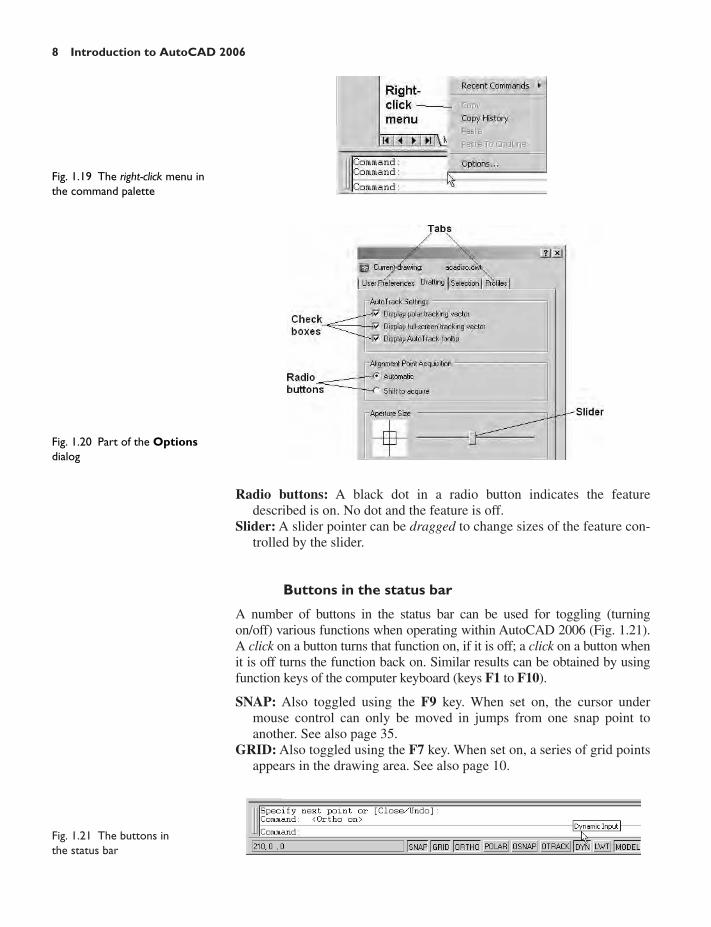
To open the Options dialog, right-click in the command palette and aright-click menu appears (Fig. 1.19). Click on the name Options . . . andthe Options dialog appears on screen. This is a complex dialog, only partof which is shown in Fig. 1.20.
Note the following in this dialog:
Tabs: A click on any of the tabs in the dialog brings a sub-dialog on screen.Check boxes: A tick appearing in a check box indicates the function
described against the box is on. No tick and the function is off. A clickin a check box toggles between the feature being off or on.
8 Introduction to AutoCAD 2006
Fig. 1.21 The buttons inthe status bar
Radio buttons: A black dot in a radio button indicates the featuredescribed is on. No dot and the feature is off.
Slider: A slider pointer can be dragged to change sizes of the feature con-trolled by the slider.
Buttons in the status bar
A number of buttons in the status bar can be used for toggling (turningon/off) various functions when operating within AutoCAD 2006 (Fig. 1.21).A click on a button turns that function on, if it is off; a click on a button whenit is off turns the function back on. Similar results can be obtained by usingfunction keys of the computer keyboard (keys F1 to F10).
SNAP: Also toggled using the F9 key. When set on, the cursor undermouse control can only be moved in jumps from one snap point toanother. See also page 35.
GRID: Also toggled using the F7 key. When set on, a series of grid pointsappears in the drawing area. See also page 10.
Fig. 1.20 Part of the Optionsdialog
Fig. 1.19 The right-click menu inthe command palette

ORTHO: Also toggled using the F8 key. When set on, lines etc. can bedrawn only vertically or horizontally.
POLAR: Also toggled using the F10 key. When set on, a small tip appearsshowing the direction and length of lines etc. in degrees and units.
OSNAP: Also toggled using the F3 key. When set on, an osnap iconappears at the cursor pick box. See also page 35.
OTRACK: When set on, lines etc. can be drawn at exact coordinatepoints and precise angles.
DYN: Dynamic Input. When set on, the x,y coordinates show as the cur-sor hairs are moved.
LWT: When set on, lineweights show on screen. When set off,lineweights show only in plotted/printed drawings.
MODEL: Toggles between Model Space and Paper Space. When inPaper Space an additional icon appears in the status bar (Fig. 1.22). Aclick on the icon maximises the drawing area. See also page 243.
Note
When constructing drawings in AutoCAD 2006 it is advisable to togglebetween Snap, Ortho, Osnap and the other functions in order to makeconstructing easier.
The AutoCAD coordinate system
In the AutoCAD 2D coordinate system, units are measured horizontally interms of X and vertically in terms of Y. A 2D point can be determined interms of X,Y (in this book referred to as x,y). x,y � 0,0 is the origin ofthe system. The coordinate point x,y � 100,50 is 100 units to the right ofthe origin and 50 units above the origin. The point x,y � �100,�50 is100 units to the left of the origin and 50 points below the origin. Fig. 1.23shows some 2D coordinate points in the AutoCAD window.
Introducing AutoCAD 2006 9
Fig. 1.22 The MaximizeViewport icon in the status bar
Fig. 1.23 2D coordinate points inthe AutoCAD coordinate system

10 Introduction to AutoCAD 2006
Drawing templates
Drawing templates are files with an extension .dwt. Templates are fileswhich have been saved with predetermined settings, such as Grid spacing,Snap spacing, etc. Templates can be opened from the Select templatedialog (see Fig. 1.18, page 7) called by clicking New . . . in the File.An example of a template file being opened is shown in Fig. 1.25. In thisexample the template is opened in Paper Space and is complete with a titleblock and borders.
When AutoCAD 2006 is used in European countries and opened, theacadiso.dwt template automatically appears on screen. Throughout thisbook drawings will usually be constructed in an adaptation of theacadiso.dwt template. To adapt this template:
1. In the command palette enter (type) grid followed by a right-click (orby pressing the Enter key). Then enter 10 in response to the promptwhich appears, followed by a right-click. (Fig. 1.26).
2. In the command palette enter snap followed by right-click. Then enter5 followed by a right-click (Fig. 1.27).
3D coordinates include a third coordinate (Z), in which positive Z unitsare towards the operator as if coming out of the monitor screen and nega-tive Z units going away from the operator as if towards the interior of thescreen. 3D coordinates are stated in terms of x,y,z. x,y,z � 100,50,50 is100 units to the right of the origin, 50 units above the origin and 50 unitstowards the operator. A 3D model drawing as if resting on the surface of amonitor is shown in Fig. 1.24.
Monitor screenY
X
Z
Fig. 1.24 A 3D model drawingshowing the X, Y and Zcoordinate directions

Introducing AutoCAD 2006 11
Fig. 1.25 A template selected foropening in the Select templatedialog
Fig. 1.26 Setting Grid to 10
Fig. 1.28 Setting Limitsto 420,297
Fig. 1.27 Setting Snap to 5
Fig. 1.29 Zooming to All
3. In the command palette enter limits, followed by a right-click. Right-click again. Then enter 420,297 and right-click (Fig. 1.28).
4. In the command window enter zoom and right-click. Then in responseto the line of prompts which appears enter a (for All) and right-click(Fig. 1.29).

5. In the command palette enter units and right-click. The Units dialogappears (Fig. 1.30). In the Precision popup list of the Length area ofthe dialog, click on 0 and then click the OK button. Note the change inthe coordinate units showing in the status bar.
12 Introduction to AutoCAD 2006
Fig. 1.30 Setting Units to 0
6. Click File in the menu bar and click Save As . . . in the drop-downmenu which appears. The Save Drawing As dialog appears. In theFiles of type popup list select AutoCAD Drawing Template (*.dwt).The templates already in AutoCAD are displayed in the dialog. Clickon acadiso.dwt, followed by another click on the Save button.
Notes
1. Now when AutoCAD is opened the template saved as acadiso.dwtautomatically loads with Grid set to 10, Snap set to 5, Limits set to420,297 (size of an A3 sheet in millimetres), with the drawing areazoomed to these limits and with Units set to 0.
2. However if other people use the computer, it is advisable to save yourtemplate to another file name, such as my_template.dwt.
3. Other features will be added to the template in future chapters.
Method of showing entries in the command palette
Throughout the book, where necessary, details entered in the commandpalette will be shown as follows:At the command line:
Command: enter zoom right-clickSpecify corner of window, enter a scale factor (nX or nXP), or
[All/Center/Dynamic/Extents/Previous/Scale/Window/Object]�real time�: enter a (All) right-click
Regenerating model.Command:

Note
In later examples this will be shortened to:
Command: enter z right-click[prompts]: enter a right-clickCommand:
Notes
1. In the above enter means type the given letter, word or words at theCommand: prompt.
2. Right-click means press the Return (right) button of the mouse.
Tools and tool icons
An important feature of Windows applications are icons and tips. In Auto-CAD 2006, tools are shown as icons in toolbars. When the cursor isplaced over a tool icon a tooltip shows with the name of the tool.
If a small arrow is included at the bottom right-hand corner of a toolicon, when the cursor is placed over the icon and the pick button of themouse depressed and held, a flyout appears which includes other toolicons (Fig. 1.31). Flyouts contain icons for tools related to the tool show-ing the arrow in its icon.
Revision notes
1. A double-click on the AutoCAD 2006 shortcut on the Windows desk-top opens the AutoCAD window.
2. Or right-click on the shortcut, followed by a left-click on Open in themenu which then appears.
3. The Standard, Layers, Properties, Styles, Draw and Modify tool-bars usually appear docked against the top or sides of the AutoCADwindow when it is opened.
4. A left-click on a menu name in the menu bar brings a drop-downmenu on screen. In drop-down menus:(a) A small outward pointing arrow against a name means that a sub-
menu will appear with a click on the name.(b) Three dots (. . .) following a name mean that a click on the name
will bring a dialog on screen.5. All constructions in this book involve the use of a mouse as the digit-
iser. When a mouse is the digitiser:(a) A left-click means pressing the left-hand button (the Pick) button.(b) A right-click means pressing the right-hand button (the Return)
button.(c) A double-click means pressing the left-hand button twice is quick
succession.(d) Dragging means moving the mouse until the cursor is over
an item on screen, holding the left-hand button down and
Introducing AutoCAD 2006 13
Fig. 1.31 Tool icons in the Drawand Modify toolbars and theLine tooltip

moving the mouse. The item moves in sympathy with the mousemovement.
(e) To pick has a similar meaning to a left-click.6. Palettes are a feature of AutoCAD 2006. In particular the Command
palette, the DesignCenter palette and the Properties palette may bein frequent use.
7. Tools are shown as icons in toolbars.8. When a tool is picked a tooltip describing the tool appears.9. A toolbar menu appears with a right-click in any toolbar on screen.
10. Dialogs allow opening and saving of files and the setting of parameters.11. A number of right-click menus are used in AutoCAD 2006.12. A number of buttons in the status bar can be used to toggle features
such as snap and grid. Function keys of the keyboard can also be usedfor toggling some of these functions.
13. The AutoCAD coordinate system determines the position in units ofany point in the drawing area and any point in 3D space.
14. Drawings are usually constructed in templates with predeterminedsettings. Some templates include borders and title blocks.
14 Introduction to AutoCAD 2006

15
CHAPTER 2
Introducing drawing
Aims of this chapter
The contents of this chapter are designed to introduce:
1. The drawing of simple outlines using the Line, Circle and Polylinetools from the Draw toolbar.
2. Drawing to snap points.3. Drawing to absolute coordinate points.4. Drawing to relative coordinate points.5. Drawing using the ‘tracking’ method.6. The use of the Erase, Undo and Redo tools.
Drawing with the Line tool
First example – Line tool (Fig. 2.3)
1. Open AutoCAD. The drawing area will show the settings of theacadiso.dwt template – Limits set to 420,297, Grid set to 10, Snapset to 5 and Units set to 0.
2. Left-click on the Line tool at the top of the Draw toolbar (Fig. 2.1).
Notes
(a) The tooltip which appears when the tool icon is clicked.(b) The prompt Command:_line Specify first point which appears
in the command window at the command line (Fig. 2.2).(c) The description of the action of the Line tool which appears at
the left-hand end of the status bar (Fig. 2.2).
Fig. 2.1 The Line tool icon in theDraw toolbar with its tooltip
Fig. 2.2 The prompts appearingat the command line in theCommand palette when Line is‘called’
3. Press the F6 key. The coordinate numbers at the left-hand end of thestatus bar either show clearly or grey out. Make sure the coordinatenumbers show clearly (black) when F6 is pressed.

16 Introduction to AutoCAD 2006
4. Make sure Snap is on by pressing either the F9 key or the SNAPbutton in the status bar. �Snap on� will show in the Commandpalette.
5. Move the mouse around the drawing area. The cursors’ pick box willjump from point to point at 5 unit intervals. The position of the pickbox will show as coordinate numbers in the status bar.
6. Move the mouse until the coordinate numbers show 60,240,0 and pressthe Pick button of the mouse (left-click).
7. Move the mouse until the coordinate numbers show 260,240,0 andleft-click.
8. Move the mouse until the coordinate numbers show 260,110,0and left-click.
9. Move the mouse until the coordinate numbers show 60,110,0 andleft-click.
10. Move the mouse until the coordinate numbers show 60,240,0and left-click. Then press the Return button of the mouse (right-click).
Fig. 2.3 appears in the drawing area.
60,240,0 260,240,0
260,110,060,110,0Fig. 2.3 First example – Line tool
Fig. 2.4 The drawing Closebutton
Second example – Line tool (Fig. 2.6)
1. Clear the drawing from the screen with a click on the drawing Close but-ton (Fig. 2.4). Make sure it is not the AutoCAD 2006 window button.
2. The warning window (Fig. 2.5) appears in the centre of the screen.Click its No button.
3. Left-click on New . . . in the File drop-down menu and from the Selecttemplate dialog which appears double-click on acadiso.dwt.
4. Left-click on the Line tool icon and enter figures as follows at eachprompt of the command line sequence:
Command:_line Specify first point: enter 80,235 right-clickSpecify next point or [Undo]: enter 275,235 right-clickSpecify next point or [Undo]: enter 295,210 right-clickSpecify next point or [Close/Undo]: enter 295,100 right-clickSpecify next point or [Close/Undo]: enter 230,100 right-click

Introducing drawing 17
Specify next point or [Close/Undo]: enter 230,70 right-clickSpecify next point or [Close/Undo]: enter 120,70 right-clickSpecify next point or [Close/Undo]: enter 120,100 right-clickSpecify next point or [Close/Undo]: enter 55,100 right-clickSpecify next point or [Close/Undo]: enter 55,210 right-clickSpecify next point or [Close/Undo]: enter c (Close) right-clickCommand:
The result is as shown in Fig. 2.6.
Fig. 2.6 Second example – Linetool
Fig. 2.5 The AutoCAD warningwindow
55,210
80,235 275,235
295,210
295,100230,100
230,70120,70
120,10055,100
Third example – Line tool (Fig. 2.7)
1. Close the drawing and open a new acadiso.dwt window.2. Left-click on the Line tool icon and enter figures as follows at each
prompt of the command line sequence:
Command:_line Specify first point: enter 60,210 right-clickSpecify next point or [Undo]: enter @50,0 right-clickSpecify next point or [Undo]: enter @0,20 right-clickSpecify next point or [Close/Undo]: enter @130,0 right-clickSpecify next point or [Close/Undo]: enter @0,�20 right-clickSpecify next point or [Close/Undo]: enter @50,0 right-clickSpecify next point or [Close/Undo]: enter @0,�105 right-clickSpecify next point or [Close/Undo]: enter @�50,0 right-clickSpecify next point or [Close/Undo]: enter @0,�20 right-clickSpecify next point or [Close/Undo]: enter @�130,0 right-clickSpecify next point or [Close/Undo]: enter @0,20 right-clickSpecify next point or [Close/Undo]: enter @�50,0 right-clickSpecify next point or [Close/Undo]: enter c (Close) right-clickCommand:
The result is as shown in Fig. 2.7.

18 Introduction to AutoCAD 2006
Fig. 2.7 Third example – Linetool
60,210@50,0
@0,20
@130,0
@0,–20
@50,0
@0,–105
@–50,0
@0,–20
@–130,0
@0,20
@–50,0
c (Close)
Notes
1. The figures typed at the keyboard determining the corners of theoutlines in the above examples are 2D x,y coordinate points. Whenworking in 2D, coordinates are expressed in terms of two numbersseparated by a comma.
2. Coordinate points can be shown as positive or as negative numbers.3. The method of constructing an outline as shown in the first two exam-
ples is known as the absolute coordinate entry method, where the x,ycoordinates of each corner of the outlines were entered at the com-mand line as required.
4. The method of constructing an outline as in the third example isknown as the relative coordinate entry method – coordinate pointsare entered relative to the previous entry. In relative coordinate entry,the @ symbol is entered before each set of coordinates with the fol-lowing rules in mind:�ve x entry is to the right.�ve x entry is to the left.�ve y entry is upwards.�ve y entry is downwards.
5. The next example (the fourth) shows how lines at angles can bedrawn taking advantage of the relative coordinate entry method.Angles in AutoCAD are measured in 360° in a counter-clockwise(anticlockwise) direction (Fig. 2.8). The � symbol precedes theangle.
Fourth example – Line tool (Fig. 2.9)
1. Close the drawing and open a new acadiso.dwt window.2. Left-click on the Line tool icon and enter figures as follows at each
prompt of the command line sequence:
Command:_line Specify first point: 70,230Specify next point: @220,0
Fig. 2.8 The counter-clockwisedirection of measuring angles inAutoCAD
0°
45°
90°
135°
180°
225°
270°
315°

Introducing drawing 19
Specify next point: @0,�70Specify next point or [Undo]: @115�225Specify next point or [Undo]: @�60,0Specify next point or [Close/Undo]: @115�135Specify next point or [Close/Undo]: @0,70Specify next point or [Close/Undo]: c (Close)Command:
The result is as shown in Fig. 2.9.
70,230 @220,0
@0,–70
@11
5 < 225
@–60,0
@115
< 135
@0,70
c (Close)
Fig. 2.9 Fourth example – Linetool
Fifth example – Line tool (Fig. 2.10)
Another method of constructing accurate drawings is by using amethod known as tracking. When Line is in use, as each Specify nextpoint: appears at the command line, a rubber-banded line appears fromthe last point entered. Drag the rubber-banded line in any direction andenter a number at the keyboard, followed by a right-click. The line isdrawn in the dragged direction of a length in units equal to the enterednumber.
In this example, because all lines are drawn in either the vertical or thehorizontal direction, either press the F8 key or click the ORTHO buttonin the status bar.
1. Close the drawing and open a new acadiso.dwt window.2. Left-click on the Line tool icon and enter figures as follows at each
prompt of the command line sequence:
Command:_line Specify first point: enter 65,220 right-clickSpecify next point: drag to right enter 240 right-clickSpecify next point: drag down enter 145 right-clickSpecify next point or [Undo]: drag left enter 65 right-clickSpecify next point or [Undo]: drag upwards enter 25 right-clickSpecify next point or [Close/Undo]: drag left enter 120 right-clickSpecify next point or [Close/Undo]: drag upwards enter 25 right-clickSpecify next point or [Close/Undo]: drag left enter 55 right-click

20 Introduction to AutoCAD 2006
Specify next point or [Close/Undo]: c (Close) right-clickCommand:
The result is as shown in Fig. 2.10.
Fig. 2.10 Fifth example – Line tool
65,220240
145
65
251202555
c (Close)
Drawing with the Circle tool
First example – Circle tool (Fig. 2.13)
1. Close the drawing just completed and open the acadiso.dwt screen.2. Left-click on the Circle tool icon in the Draw toolbar (Fig. 2.11).3. Type numbers against the prompts appearing in the command window
as shown in Fig. 2.12, followed by right-clicks. The circle (Fig. 2.13)appears on screen.
Fig. 2.11 The Circle tool icon inthe Draw toolbar with its tooltip
Fig. 2.12 First example – Circle.The command line prompts whenCircle is called
180,160
R55
Fig. 2.13 First example – Circletool
Second example – Circle tool (Fig. 2.11)
1. Close the drawing and open the acadiso.dwt screen.2. Left-click on the Circle tool icon and construct two circles as shown in
the drawing Fig. 2.14.
Fig. 2.14 Second example – Circletool. The two circles of radius 50

Introducing drawing 21
3. Click the Circle tool again and against the first prompt enter t (theabbreviation for the prompt tan tan radius), followed by a right-click.
Command:_circle Specify center point for circle or [3P/2P/Ttr (tantan radius)]: enter t right-click
Specify point on object for first tangent of circle: pickSpecify point on object for second tangent of circle: pickSpecify radius of circle (50): enter 40 right-clickCommand:
The radius 40 circle, tangential to the two already drawn circles, thenappears (Fig. 2.15)
Fig. 2.15 The radius 40 circletangential to the radius 50 circles
Fig. 2.16 The Erase tool iconand its tooltip at the top of the Modify toolbar
100,160 240,160
R50
R40
R50
+ +
Notes
1. When a point on either circle is picked a tip appears Deferred Tan-gent. This tip will appear only when the OSNAP is set on with a clickon the button, or the F3 key of the keyboard is pressed.
2. Circles can be drawn through 3 points or through 2 points entered atthe command line in response to prompts brought to the command lineby using 3P and 2P in answer to the circle command line prompts.
The Erase tool
If an error has been made when using any of the AutoCAD 2006 tools,the object or objects which have been incorrectly constructed canbe deleted with the Erase tool. The Erase tool icon is at the top of theModify toolbar (Fig. 2.16).
First example – Erase (Fig. 2.18)
1. With Line tool construct the outline in Fig. 2.17.2. Assuming two lines of the outline have been incorrectly drawn, left-
click the Erase tool icon. The command line shows:
Command:_eraseSelect objects: pick one of the linesSelect objects: pick the other lineSelect objects: right-clickCommand:

22 Introduction to AutoCAD 2006
And the two lines are deleted (right-hand drawing of Fig. 2.18).
90,255
130 40
3590
35Fig. 2.17 First example – Erase.An incorrect outline
Fig. 2.18 First example – Erase
Select objects Result after Erase
Second example – Erase (Fig. 2.19)
The two lines could also have been deleted by the following method:
1. Left-click the Erase tool icon. The command line shows:
Command:_eraseSelect objects: enter c (Crossing)Specify first corner: pick Specify opposite corner: pick 2 foundSelect objects: right-clickCommand:
And the two lines are deleted as in the right-hand drawing of Fig. 2.18.
first corner
opposite corner
Fig. 2.19 Second example – Erase

Introducing drawing 23
Undo and Redo tools
Two other tools of value when errors have been made are the Undo andRedo tools. To undo the last action taken by any tool when constructing adrawing, either left-click the Undo tool (Fig. 2.20) or type u at the com-mand line. No matter which method is adopted the error is deleted fromthe drawing.
Fig. 2.20 The Undo tool in theStandard toolbar
Everything constructed during a session in constructing a drawing canbe undone by repeated clicking on the Undo tool icon or by entering u’sat the command line.
To bring back objects that have been removed by the use of Undos,left-click the Redo tool icon (Fig. 2.21) or enter redo at the commandline.
Drawing with the Polyline tool
Possibly the most versatile of the tools from the Draw toolbar. Whendrawing lines with the Line tool, each line drawn is an object in its ownright, so a rectangle drawn with the Line tool is made up of four objects.But, a rectangle drawn with the Polyline tool is a single object. Lines ofdifferent thickness, arcs, arrows and circles can all be drawn using thistool as will be shown in the examples describing constructions using thePolyline tool. Constructions resulting from using the tool are known aspolylines or plines.
To call the Polyline tool for use, left-click on its tool icon from theDraw toolbar (Fig. 2.22).
First example – Polyline tool (Fig. 2.23)
Note
In this example enter and right-click have been left out from the com-mand line responses.Left-click the Polyline tool (Fig. 2.22). The command line shows:
Command:_pline Specify start point: 30,250Current line width is 0Specify next point or [Arc/Halfwidth/Length/Undo/Width]: 230,250Specify next point or [Arc/Close/Halfwidth/Length/Undo/Width]:
230,120
Fig. 2.21 The Redo tool in theStandard toolbar
Fig. 2.22 The Polyline tool fromthe Draw toolbar
24 Introduction to AutoCAD 2006
Specify next point or [Arc/Close/Halfwidth/Length/Undo/Width]:30,120
Specify next point or [Arc/Close/Halfwidth/Length/Undo/Width]:c (Close)
Command:
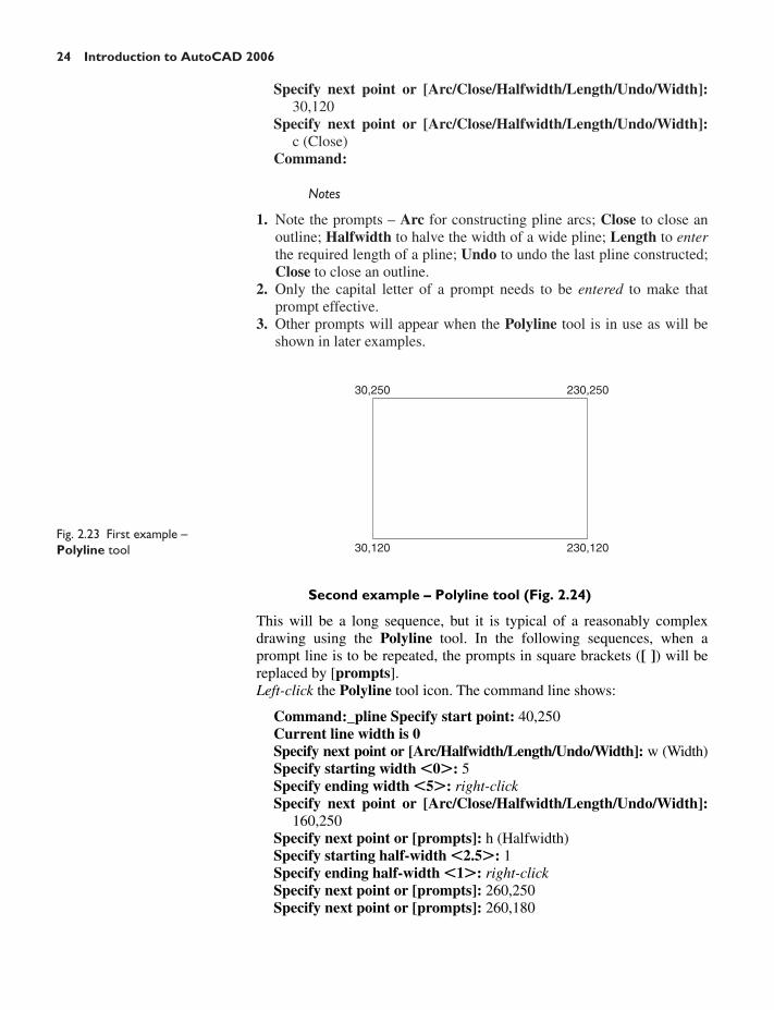
Notes
1. Note the prompts – Arc for constructing pline arcs; Close to close anoutline; Halfwidth to halve the width of a wide pline; Length to enterthe required length of a pline; Undo to undo the last pline constructed;Close to close an outline.
2. Only the capital letter of a prompt needs to be entered to make thatprompt effective.
3. Other prompts will appear when the Polyline tool is in use as will beshown in later examples.
Fig. 2.23 First example –Polyline tool
30,250 230,250
230,12030,120
Second example – Polyline tool (Fig. 2.24)
This will be a long sequence, but it is typical of a reasonably complexdrawing using the Polyline tool. In the following sequences, when aprompt line is to be repeated, the prompts in square brackets ([ ]) will bereplaced by [prompts].Left-click the Polyline tool icon. The command line shows:
Command:_pline Specify start point: 40,250Current line width is 0Specify next point or [Arc/Halfwidth/Length/Undo/Width]: w (Width)Specify starting width �0�: 5Specify ending width �5�: right-clickSpecify next point or [Arc/Close/Halfwidth/Length/Undo/Width]:
160,250Specify next point or [prompts]: h (Halfwidth)Specify starting half-width �2.5�: 1Specify ending half-width �1�: right-clickSpecify next point or [prompts]: 260,250Specify next point or [prompts]: 260,180

Introducing drawing 25
Specify next point or [prompts]: w (Width)Specify starting width �1�: 10Specify ending width �10�: right-clickSpecify next point or [prompts]: 260,120Specify next point or [prompts]: h (Halfwidth)Specify starting half-width �5�: 2Specify ending half-width �2�: right-clickSpecify next point or [prompts]: 160,120Specify next point or [prompts]: w (Width)Specify starting width �4�: 20Specify ending width �20�: right-clickSpecify next point or [prompts]: 40,120Specify starting width �20�: 5Specify ending width �5�: right-clickSpecify next point or [prompts]: cl (CLose)Command:
40,250 160,250 260,250
260,180
260,120160,12040,120
Fig. 2.24 Second example –Polyline tool
Third example – Polyline tool (Fig. 2.25)
Left-click the Polyline tool icon. The command line shows:
Command:_pline Specify start point: 50,220Current line width is 0[prompts]: w (Width)Specify starting width �0�: 0.5Specify ending width �0.5�: right-clickSpecify next point or [prompts]: 120,220Specify next point or [prompts]: a (Arc)Specify endpoint of arc or [prompts]: s (second pt)Specify second point on arc: 150,200Specify end point of arc: 180,220Specify end point of arc or [prompts]: l (Line)Specify next point or [prompts]: 250,220Specify next point or [prompts]: 250,190Specify next point or [prompts]: a (Arc)Specify endpoint of arc or [prompts]: s (second pt)Specify second point on arc: 240,170

26 Introduction to AutoCAD 2006
Specify end point of arc: 250,150Specify end point of arc or [prompts]: l (Line)Specify next point or [prompts]: 250,150Specify next point or [prompts]: 250,120Command:
And so on until the outline Fig. 2.25 is completed.
Fig. 2.25 Third example –Polyline tool
50,220 120,220
150,200
180,220 250,220
250,190
240,170
250,150
250,120180,120
150,140
120,12050,120
50,150
60,170
50,190
Fourth example – Polyline tool (Fig. 2.26)
Left-click the Polyline tool icon. The command line shows:
Command:_pline Specify start point: 80,170Current line width is 0Specify next point or [prompts]: w (Width)Specify starting width �0�: 1Specify ending width �1�: right-clickSpecify next point or [prompts]: a (Arc)Specify endpoint of arc or [prompts]: s (second pt)Specify second point on arc: 160,250Specify end point of arc: 240,170Specify end point of arc or [prompts]: cl (CLose)Command:
And the circle in Fig. 2.26 is formed.
Fig. 2.26 Fourth example –Polyline tool
80,170
160,250
240,170

Introducing drawing 27
Fifth example – Polyline tool (Fig. 2.27)
Left-click the Polyline tool icon. The command line shows:
Command:_pline Specify start point: 60,180Current line width is 0Specify next point or [prompts]: w (Width)Specify starting width �0�: 1Specify ending width �1�: right-clickSpecify next point or [prompts]: 190,180Specify next point or [prompts]: w (Width)Specify starting width �1�: 20Specify ending width �20�: 0Specify next point or [prompts]: 265,180Specify next point or [prompts]: right-clickCommand:
And the arrow in Fig. 2.27 is formed.
Fig. 2.27 Fifth example –Polyline tool
60,180
Width = 20
190,180265,180Width = 0Width = 1
Revision notes
The following terms have been used in this chapter:
Left-click – press the left-hand button of the mouse.Click – same meaning as left-click.Double-click – press the left-hand button of the mouse twice in quick
succession.Right-click – press the right-hand button of the mouse; it has the same
result as pressing the Return key of the keyboard.Drag – move the cursor on to an object and, holding down the right-hand
button of the mouse, pull the object to a new position.Enter – type the letters, or numbers which follow at the keyboard.Pick – move the cursor on to an item on screen and press the left-hand
button of the mouse.Return – press the Enter key of the keyboard. This key may also be
marked with a left-facing arrow. In most cases (but not always) has thesame result as a right-click.
Dialog – a window appearing in the AutoCAD window in which settingscan be made.
Drop-down menu – a menu appearing when one of the names in themenu bars is clicked.
Tooltip – the name of a tool appearing when the cursor is placed over atool icon from a toolbar.
Prompts – text appearing in the command window when a tool isselected, which advise the operator as to which operation is required.

28 Introduction to AutoCAD 2006
Methods of coordinate entry – Three methods of coordinate entry havebeen used in this chapter:1. Absolute method – the coordinates of points on an outline are
entered at the command line in response to prompts.2. Relative method – the distances in coordinate units are entered
preceded by @ from the last point which has been determined onan outline. Angles which are measured in a counter-clockwisedirection are preceded by �.
3. Tracking – the rubber band of the tool is dragged in the directionin which the line is to be drawn and its distance in units is enteredat the command line followed by a right-click.
Line and Polyline tools – an outline drawn using the Line tool consistsof a number of objects equal to the number of lines in the outline. Anoutline drawn using the Polyline is a single object no matter how manyplines are in the outline.
Exercises
1. Using the Line tool construct the rectangle in Fig. 2.28.
40,250 270,250
40,100 270,100Fig. 2.28 Exercise 1
Fig. 2.29 Exercise 2
195
120
2. Construct the outline in Fig. 2.29 using the Line tool. The coordinatepoints of each corner of the rectangle will need to be calculated fromthe lengths of the lines between the corners.

Introducing drawing 29
3. Using the Line tool, construct the outline in Fig. 2.30.
Fig. 2.30 Exercise 3
140
90
225°
315°
45°
135°
6060
6060
4. Using the Circle tool, construct the two circles of radius 50 and 30.Then using the Ttr prompt add the circle of radius 25 (Fig. 2.31).
R30
R25R50
100,170 200,170
Fig. 2.31 Exercise 4
5. Fig. 2.32. In an acadiso.dwt screen, using the Circle and Line tools,construct the line and the circle of radius 40. Then, using the Ttrprompt, add the circle of radius 25.
Fig. 2.32 Exercise 5
50,130
200,190
185
R25
R40
6. Using the Line tool, construct the two lines at the length and angle asgiven in Fig. 2.33. Then with the Ttr prompt of the Circle tool, addthe circle as shown.

30 Introduction to AutoCAD 2006
7. Using the Polyline tool, construct the outline given in Fig. 2.34.
110,210 180,210250,21050,210
Width = 2
Width = 2
Width = 20
Width = 30Width = 10
Width = 10
Width = 10
Width = 2
50,105 250,105110,105 180,105Fig. 2.35 Exercise 8
Fig. 2.36 Exercise 9
Fig. 2.33 Exercise 6
Fig. 2.34 Exercise 7
100
120°
130
R40
20 20 3012030
2080
2020
20
260
20Polyline width = 1.5
8. Construct the outline in Fig. 2.35 using the Polyline tool.
9. With the Polyline tool construct the arrows shown in Fig. 2.36.

31
CHAPTER 3
Osnap, AutoSnap andDraw tools
Aims of this chapter
1. To describe the uses of the Arc, Ellipse, Polygon and Rectangle toolsfrom the Draw toolbar.
2. To describe the uses of the Polyline Edit (pedit) tool.3. To introduce the AutoSnap system and its uses.4. To introduce the Object Snap (osnap) system and it uses.
Introduction
The majority of tools in AutoCAD 2006 can be called into use in thefollowing four ways:
1. With a click on the tool’s icon in its toolbar.2. By clicking on the tool’s name in an appropriate drop-down menu.
Fig. 3.1 shows the tool names displayed in the Draw drop-downmenu.
3. By entering an abbreviation for the tool name at the command line inthe Command palette. For example the abbreviation for the Line toolis l, for the Polyline tool it is pl and for the Circle tool it is c.
4. By entering the full name of the tool at the command line.
In practice operators constructing drawings in AutoCAD 2006 maywell use a combination of these four methods.
The Arc tool
In AutoCAD 2006, arcs can be constructed using any three of the followingcharacteristics of an arc: Its Start point; a point on the arc (Second point);its Center; its End; its Radius; Length of the arc; Direction in which thearc is to be constructed; Angle between lines of the arc.
In the examples which follow, entering initials for these characteristics,in response to prompts at the command line when the Arc tool is called,allows arcs to be constructed in a variety of ways.
To call the Arc tool click on its tool icon in the Draw toolbar (Fig. 3.2),or click on Arc in the Draw drop-down menu. A sub-menu shows thepossible methods of constructing arcs (Fig. 3.3). The abbreviation for callingthe Arc tool is a.
Fig. 3.1 The tool names in theDraw drop-down menu
Fig. 3.2 The Arc tool icon in theDraw toolbar

32 Introduction to AutoCAD 2006
First example – Arc tool (Fig. 3.4)
Left-click the Arc tool icon. The command line shows:
Command:_arc Specify start point of arc or [Center]: 100,220Specify second point of arc or [Center/End]: 55,250Specify end point of arc: 10,220Command:
Second example – Arc tool (Fig. 3.4)
Command: right-click brings back the Arc sequenceARC Specify start point of arc or [Center]: c (Center)Specify center point of arc: 200,190Specify start point of arc: 260,215Specify end point of arc or [Angle/chord Length]: 140,215Command:
Fig. 3.3 The Arc sub-menu of theDraw drop-down menu
10,220
55,250
100,220First example Center is 200,190
Second example
260,215140,215 420,210320,210Radius = 75
Third exampleFig. 3.4 Examples – Arc tool
Osnap, AutoSnap and Draw tools 33
Fig. 3.5 An ellipse can be regardedas viewing a rotated circle
Ellipse as seen from
direction of arrow
Major axis Minor axis
Circle asseen from
a side
Circle as seen from direction
of arrow
Diameter
Circle rotated through 60°
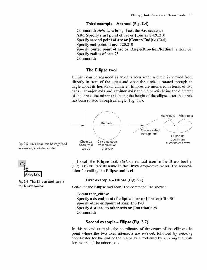
Third example – Arc tool (Fig. 3.4)
Command: right-click brings back the Arc sequenceARC Specify start point of arc or [Center]: 420,210Specify second point of arc or [Center/End]: e (End)Specify end point of arc: 320,210Specify center point of arc or [Angle/Direction/Radius]: r (Radius)Specify radius of arc: 75Command:
The Ellipse tool
Ellipses can be regarded as what is seen when a circle is viewed fromdirectly in front of the circle and when the circle is rotated through anangle about its horizontal diameter. Ellipses are measured in terms of twoaxes – a major axis and a minor axis; the major axis being the diameterof the circle, the minor axis being the height of the ellipse after the circlehas been rotated through an angle (Fig. 3.5).
Fig. 3.6 The Ellipse tool icon inthe Draw toolbar
To call the Ellipse tool, click on its tool icon in the Draw toolbar(Fig. 3.6) or click its name in the Draw drop-down menu. The abbrevi-ation for calling the Ellipse tool is el.
First example – Ellipse (Fig. 3.7)
Left-click the Ellipse tool icon. The command line shows:
Command:_ellipseSpecify axis endpoint of elliptical arc or [Center]: 30,190Specify other endpoint of axis: 150,190Specify distance to other axis or [Rotation]: 25Command:
Second example – Ellipse (Fig. 3.7)
In this second example, the coordinates of the centre of the ellipse (thepoint where the two axes intersect) are entered, followed by enteringcoordinates for the end of the major axis, followed by entering the unitsfor the end of the minor axis.

34 Introduction to AutoCAD 2006
Command: right-clickELLIPSESpecify axis endpoint of elliptical arc or [Center]: c (Center)Specify center of ellipse: 260,190Specify endpoint of axis: 205,190Specify distance to other axis or [Rotation]: 30Command:
Third example – Ellipse (Fig. 3.7)
In this third example, after setting the positions of the ends of the majoraxis, the angle of rotation of the circle from which an ellipse can beobtained is entered.
Command: right-clickELLIPSESpecify axis endpoint of elliptical arc or [Center]: 30,100Specify other endpoint of axis: 120,100Specify distance to other axis or [Rotation]: r (Rotation)Specify rotation around major axis: 45Command:
Saving drawings
Before going further it is as well to know how to save the drawings con-structed when answering examples and exercises in this book. When adrawing has been constructed, left-click on File in the menu bar and onSave As . . . in the drop-down menu (Fig. 3.8). The Save Drawing As dia-log appears (Fig. 3.9).
Unless you are the only person to use the computer on which the draw-ing has been constructed, it is best to save work to a floppy disk, usuallyheld in the drive A:. To save a drawing to a floppy in drive A:
1. Place a floppy disk in drive A:.2. In the Save in: field of the dialog, click the arrow to the right of the
field and from the popup list select 31⁄2 Floppy [A:].
30,190
First example
150,190
30,100 Rotation = 45° 120,100
205,190
Second example
260,190
30
Third example
25
Fig. 3.7 Examples – Ellipse

Osnap, AutoSnap and Draw tools 35
Fig. 3.9 The Save Drawing Asdialog
Fig. 3.8 Selecting Save As . . . inthe File drop-down menu
3. In the File name: field of the dialog, type a suitable name. The file nameextension .dwg does not need to be typed because it will automaticallybe added to the file name.
4. Left-click the Save button of the dialog. The drawing will be saved tothe floppy with the file name extension .dwg – the AutoCAD file nameextension.
Osnap, AutoSnap and Dynamic Input
In previous chapters several methods of constructing accurate drawingshave been described – using Snap; absolute coordinate entry; relativecoordinate entry and tracking.

Other methods of ensuring accuracy between parts of constructions areby making use of Object Snaps (Osnaps), AutoSnap and DynamicInput (DYN).
Snap, Grid, Osnap and DYN can be set from the buttons in the status baror by pressing the keys F3 (Osnap), F7 (Grid), F9 (Snap) and F12 (DYN).
Object Snaps (Osnaps)
Osnaps allow objects to be added to a drawing at precise positions in rela-tion to other objects already on screen. With osnaps, objects can be addedto the end points, mid points, to intersections of objects, to centres andquadrants of circles and so on. Osnaps also override snap points evenwhen snap is set on.To set Osnaps, at the command line:
Command: enter os
And the Drafting Settings dialog appears. Click the Object Snap tab inthe upper part of the dialog and click in each of the check boxes (the smallsquares opposite the osnap names). See Fig. 3.10.
36 Introduction to AutoCAD 2006
When osnaps are set ON, as outlines are constructed using osnaps,osnap icons and their tooltips appear as indicated in Fig. 3.11.
It is sometimes advisable not to have Osnaps set on in the DraftingSettings dialog, but to set Osnap off and use osnap abbreviations at the
Fig. 3.10 The Drafting Settingsdialog with some Osnaps set on

Osnap, AutoSnap and Draw tools 37
command line when using tools. The following examples show the use ofsome of these abbreviations.
First example – Osnap abbreviations (Fig. 3.12)
Call the Polyline tool:
Command:_plineSpecify start point: 50,230[prompts]: w (Width)Specify starting width: 1Specify ending width <1>: right-clickSpecify next point: 260,230Specify next point: right-clickCommand: right-clickPLINESpecify start point: enter end right-clickof pick the right-hand end of the plineSpecify next point: 50,120Specify next point: right-clickCommand: right-clickPLINESpecify start point: enter mid right-clickof pick near the middle of first plineSpecify next point: 155,120Specify next point: right-clickCommand: right-clickPLINESpecify start point: enter int right-clickof pick the plines at their intersectionSpecify start point: right-clickCommand:
The result is as shown in Fig. 3.12. In this illustration the osnap tooltipsare shown as they appear when each object is added to the outline.
Fig. 3.11 Three osnap icons andtheir tooltips

38 Introduction to AutoCAD 2006
Second example – Osnap abbreviations (Fig. 3.13)
Call the Circle tool:
Command:_circleSpecify center point for circle: 180,170Specify radius of circle: 60Command: enter l (Line) right-clickSpecify first point: enter qua right-clickof pick near the upper quadrant of the circleSpecify next point: enter cen right-clickof pick near the centre of the circleSpecify next point: enter qua right-clickof pick near right-hand side of circleSpecify next point: right-clickCommand:
Note
With osnaps off, the following abbreviations can be used:
end endpointint intersectionqua quadrantext extensionmid midpointcen centrenea nearest
AutoSnap
AutoSnap is similar to Osnap. To set AutoSnap, right-click in the com-mand window and from the menu which appears click Options . . . TheOptions dialog appears. Click the Drafting tab in the upper part of thedialog and set the check boxes against the AutoSnap Settings on (tick inboxes). These settings are shown in Fig. 3.14.
With AutoSnap set, each time an object is added to a drawing theAutoSnap features appear as indicated in Fig. 3.15.
Fig. 3.12 First example – Osnaps

Osnap, AutoSnap and Draw tools 39
Fig. 3.13 Second example –Osnaps
Fig. 3.15 The features ofAutoSnap
Fig. 3.14 Setting AutoSnap inthe Options dialog

Part of a drawing showing the features of a number of AutoSnappoints is given in Fig. 3.16.
40 Introduction to AutoCAD 2006
Note
OSNAP must be set ON for the AutoSnap features to show when con-structing a drawing with their aid.
Dynamic Input
A click on the DYN button in the status bar, or pressing the key F12brings Dynamic Input into operation. When DYN is set on by eitherpressing the F12 key or with a click on the DYN button in the status bar,dimensions, coordinate positions and commands appear as tips when atool is in action (Fig. 3.17).
With no tool in action as the cursor hairs are moved in response tomovement of the mouse, DYN tips showing the coordinate figures for thepoint of the cursor hairs will show (Fig. 3.18).
Setting for DYN can be made in the Drafting Settings dialog(Fig. 3.19), brought to screen by entering ds at the command line.
Example – using Polyline with DYN
1. Click the DYN button in the status bar to set dynamic input on.2. At the command line:
Command: enter commandlinehide right-clickAnd the Hide Command Line Window (Fig. 3.20) appears.
3. Click the Yes button of the dialog. The command palette disappears.This has the advantage of providing a larger drawing area.
Fig. 3.16 A number of AutoSnapfeatures

Osnap, AutoSnap and Draw tools 41
Fig. 3.17 The DYN tips appearingwhen a tool is in action – in thisexample the Polyline tool
Fig. 3.18 Coordinate tips whenDYN is in action
Fig. 3.19 Setting for DYN can bemade in the Drafting Settingsdialog
Fig. 3.20 The Hide CommandLine Window

42 Introduction to AutoCAD 2006
4. Click the Polyline tool in the Draw toolbar or enter pl at the keyboard.The DYN tips show as in Fig. 3.21.
5. Type w (Width), followed by 2 and right-click. Enter 2 again. The tipsshow as in Fig. 3.22. Then right-click.
6. Drag the cursor to the right and type 115. The tips show as in Fig. 3.23.7. Continue in this manner until a required outline is drawn.
Fig. 3.24 The Polygon tool iconin the Draw toolbar
Fig. 3.21 Example – usingPolyline with DYN – stage 1
Fig. 3.22 Example – usingPolyline with DYN – stage 2
Fig. 3.23 Example – usingPolyline with DYN – stage 3
Notes
1. It will be seen from this example that a knowledge of the promptswhich appears at the command line when a tool is in use will berequired to make full use of the Dynamic Input system.
2. The advantage of using DYN is twofold – the command palette can behidden allowing more drawing area space and there is no need to keeplooking down at the command line.
3. However for those new to AutoCAD it is necessary to learn the commandline prompts. Thus throughout this book the command line promptssequences are shown. When the operator is conversant with the promptsthey may decide to use the DYN method in preference to using the com-mand palette.
4. The command palette can be brought back to screen either by pressingthe Ctrl�9 keys or by typing commandline at the keyboard.
Examples of using some Draw tools
First example – Polygon tool (Fig. 3.25)
1. Call the Polygon tool – either with a click on its tool icon in the Drawtoolbar (Fig. 3.24), or by entering pol or polygon at the command line,or from the Draw drop-down menu. The command line shows:
Command:_polygon Enter number of sides �4�: 6Specify center of polygon or [Edge]: 60,210Enter an option [Inscribed in circle/Circumscribed about circle]
�I�: right-click (accept Inscribed)Specify radius of circle: 60Command:
2. In the same manner construct a 5-sided polygon of centre 200,210 andradius 60.
3. Then, construct an 8-sided polygon of centre 330,210 and radius 60.

Osnap, AutoSnap and Draw tools 43
4. Repeat to construct a 9-sided polygon circumscribed about a circle ofradius 60 and centre 60,80.
5. Construct yet another polygon with 10 sides of radius 60 and centre200,80.
6. Finally another polygon circumscribing a circle of radius 60, centre330,80 and sides 12.
The result is shown in Fig. 3.25.
6-sided hexagon
5-sided pentagon
8-sidedoctagon
9-sided nanogon
10-sided decagon
12-sided duodecagon
Inscribing circle
Circumscribing circle
Fig. 3.25 First example –Polygon tool
Fig. 3.26 The Rectangle tool inthe Draw toolbar
Second example – Rectangle tool (Fig. 3.27)
Call the Rectangle tool – either with a click on its tool icon in the Drawtoolbar (Fig. 3.26), or by entering rec or rectang at the command line, orfrom the Draw drop-down menu. The command line shows:
Command:_rectangSpecify first corner point or [Chamfer/Elevation/Fillet/Thickness/
Width]: 25,240Specify other corner point or [Dimensions]: 160,160Command:
Third example – Rectangle tool (Fig. 3.27)
Command:_rectang[prompts]: c (Chamfer)Specify first chamfer distance for rectangles �0�: 15Specify first chamfer distance for rectangles �15�: right-clickSpecify first corner point: 200,240Specify other corner point: 300,160Command:
Fourth example – Rectangle (Fig. 3.27)
Command: _rectangSpecify first corner point or [Chamfer/Elevation/Fillet/Thickness/
Width]: w (Width)

44 Introduction to AutoCAD 2006
Fig. 3.28 Calling Edit Polylinefrom the Modify II toolbar
Fig. 3.29 Calling Polyline Editfrom the Modify drop-down menu
Fig. 3.27 Examples – Rectangletool
25,240
160,160
200,240
300,160
Chamfers15 and 15
Width = 2 Fillet = R15
20,120
160,30
200,120
315,25
Width = 4 Chamfers 10 and 15
Specify line width for rectangles �0�: 4Specify first corner point or [Chamfer/Elevation/Fillet/Thickness/
Width]: c (Chamfer)Specify first chamfer distance for rectangles �0�: 10Specify second chamfer distance for rectangles �10�: 15Specify first corner point or [Chamfer/Elevation/Fillet/Thickness/
Width]: 200, 120Specify other corner point or [Area/Dimensions/Rotation]: 315, 25Command:
The Polyline Edit tool
Polyline Edit or Pedit is a valuable tool for editing plines.
First example – Polyline Edit (Figs 3.30 and 3.31)
1. With the Polyline tool construct the outlines 1 to 6 of Fig. 3.30.2. Call the Edit Polyline tool – either with a click on its tool icon in the
Modify II toolbar (Fig. 3.28), or by entering pe or pedit at the com-mand line, or from the Modify drop-down menu (Fig. 3.29).
By far the easiest method of calling the tool is to enter pe at thecommand line. The command line shows:
Command: enter pePEDIT Select polyline or [Multiple]: pick pline 2

Osnap, AutoSnap and Draw tools 45
Fig. 3.30 Example – PolylineEdit
Pline rectangle120 × 80
1 2 3
4 5 6
1
Pline 120 × 80 of Width = 0
Pedit to Width = 2 Pedit to Width = 10
Pedit using the Spline prompt
Pline with open side Pedit drawing 5 using Close
2 3
654
Fig. 3.31 Example – PolylineEdit
Enter an option [Open/Join/Width/Edit vertex/Fit/Spline/Decurve/Ltype gen/Undo]: w (Width)
Specify new width for all segments: 2Enter an option [Open/Join/Width/Edit vertex/Fit/Spline/Decurve/
Ltype gen/Undo]: right-clickCommand:
3. Repeat with pline 3 and pedit to Width � 10.4. Repeat with pline 4 and enter s (Spline) in response to the prompt line:
Enter an option [Open/Join/Width/Edit vertex/Fit/Spline/Decurve/Ltype gen/Undo]:
5. Repeat with pline 5 and enter j (Join) in response to the prompt line:
Enter an option [Open/Join/Width/Edit vertex/Fit/Spline/Decurve/Ltype gen/Undo]:
The result is shown in pline 6.

46 Introduction to AutoCAD 2006
Example – Multiple Polyline Edit (Fig. 3.32)
1. With the Line and Arc tools construct the left-hand outlines of Fig. 3.32.2. Call the Edit Polyline tool. The command line shows:
Command: enter pePEDIT Select polyline or [Multiple]: enter m (Multiple)Select objects: pick any one of the lines or arcs of Fig. 3.32.1 foundSelect objects: pick another line or arc 1 found, 2 total
Continue selecting lines and arcs as shown by the pick boxes of the left-hand drawing of Fig. 3.32 until the command line shows:
Select objects: pick another line or arc 1 found, 24 totalSelect objects: right-clickConvert Lines and Arcs to polylines [Yes/No]? <Y>: right-click[prompts] enter w right-clickSpecify new width for all segments: enter 2 right-click[prompts]: right-clickCommand:
The result is shown in the right-hand drawing of Fig. 3.32.
Fig. 3.32 Example – MultiplePolyline Edit
pick
2030
6030
20
2020602020
100
80
Outlines using Line and Arc
After Multiple Peditto Width = 2
15
15
Transparent commands
When any tool is in operation it can be interrupted by prefixing the inter-rupting command with an apostrophe (’). This is particularly usefulwhen wishing to zoom when constructing a drawing (see page 52). As anexample when the Line tool is being used:
Command:_lineSpecify first point: 100,120Specify next point: 190,120Specify next point: enter ’z (Zoom)

Osnap, AutoSnap and Draw tools 47
�� Specify corner of window or [prompts]: pick����Specify opposite corner: pickResuming line command.Specify next point:
And so on. The transparent command method can be used with any tool.
The set variable PELLIPSE
Many of the operations performed in AutoCAD are carried out under thesettings of set variables. Some of the numerous set variables available inAutoCAD 2006 will be described in later pages. The variable PELLIPSEcontrols whether ellipses are drawn as splines or as polylines. It is set asfollows:
Command: enter pellipse right-clickEnter new value for PELLIPSE �0�: enter 1 right-clickCommand:
And now when ellipses are drawn they are plines. If the variable is set to 0,the ellipses will be splines.
Revision notes
The following terms have been used in this chapter:
Field – a part of a window or dialog in which numbers or letters areentered or can be read.
Popup list – a list brought in screen with a click on the arrow often foundat the right-hand end of a field.
Object – a part of a drawing which can be treated as a single object. Forexample a line constructed with the Line tool is an object; a rectangleconstructed with the Polyline tool is an object; an arc constructedwith the Arc tool is an object. It will be seen in a later chapter (Chap-ter 9) that several objects can be formed into a single object.
Toolbar – a collection of tool icons, all of which have similar functions.For example the Draw toolbar contains tool icons of tools which areused for drawing. The Modify toolbar contains tool icons of tools usedfor modifying parts of drawings.
Command line – a line in the command window which commences withthe word Command:.
Snap, Grid and Osnap can be toggled with clicks on the buttons in the sta-tus bar. These functions can also be set with function keys: Snap – F9;Grid – F7 and Osnap – F3.
Osnaps ensure accurate positioning of objects in drawings.AutoSnap can also be used for ensuring accurate positioning of objects in
relation to other objects in a drawing.Osnap must be set ON before AutoSnap can be used.Osnap abbreviations can be used rather than be set from the Drafting
Settings dialog.

48 Introduction to AutoCAD 2006
Notes on tools
1. Polygons constructed with the Polygon tool are regular polygons – theedges of the polygons all are the same length and the angles are of thesame degrees.
2. Polygons constructed with the Polygon tool are plines, so can be actedupon with the Edit Polyline tool.
3. Rectangles constructed with the Rectangle tool are plines. They canbe drawn with chamfers or fillets and their width can be varied.
4. The Edit Polyline tool can be used to change plines.5. The easiest method of calling the Edit Polyline tool is to enter pe at
the command line.6. The Multiple prompt of the pedit tool saves considerable time when
editing a number of objects in a drawing.7. Transparent commands can be used to interrupt tools in operation by
preceding the interrupting tool name with an apostrophe (’).8. Ellipses drawn when the variable PELLIPSE is set to 0 are splines;
when PELLIPSE is set to 1, ellipses are polylines.
Exercises
1. Using the Line and Arc tools, construct the outline given inFig. 3.33.
80,250 260,250
260,230
230,160
260,90
260,70Fig. 3.33 Exercise 1
2. With the Line and Arc tools, construct the outline given in Fig. 3.34.3. Using the Ellipse and Arc tools construct the drawing in Fig. 3.35.4. With the Line, Circle and Ellipse tools construct Fig. 3.36.5. With the Ellipse tool, construct the drawing in Fig. 3.376. Fig. 3.38 shows a rectangle in the form of a square with hexagons
along each edge. Using the Dimensions prompt of the Rectangle toolconstruct the square. Then, using the Edge prompt of the Polygontool, add the four hexagons. Use the Osnap endpoint to ensure thepolygons are in their exact positions.

Osnap, AutoSnap and Draw tools 49
80,230 290,230
290,7580,75
R130R130
40Fig. 3.35 Exercise 3
Fig. 3.36 Exercise 4
240
20
2015
0
Ø20
150
Fig. 3.34 Exercise 2
90,210 260,210
260,70
260,9090,90
90,70
260,19090,190
R135
R70 R70
R135
7. Fig. 3.39 shows seven hexagons with edges touching. Construct theinner hexagon using the Polygon tool, then with the aid of the Edgeprompt of the tool, add the other six hexagons.
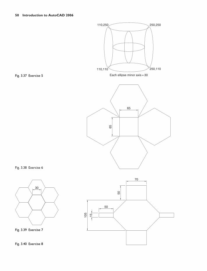
8. Fig. 3.40 was constructed using only the Rectangle tool. Make anexact copy of the drawing using only the Rectangle tool.
50 Introduction to AutoCAD 2006
Fig. 3.38 Exercise 6
6565
30
Fig. 3.39 Exercise 7
Fig. 3.40 Exercise 8
70
50
105
50
15
250,250
250,110
110,250
110,110
Each ellipse minor axis = 30Fig. 3.37 Exercise 5
Osnap, AutoSnap and Draw tools 51
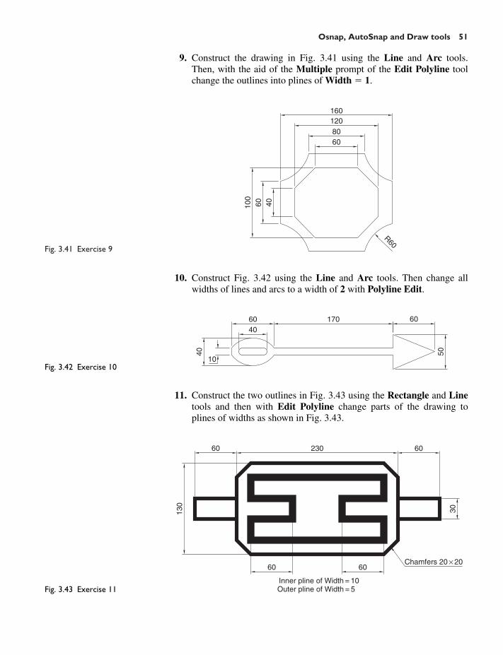
Fig. 3.41 Exercise 9
1601208060
100
60 40
R60
9. Construct the drawing in Fig. 3.41 using the Line and Arc tools.Then, with the aid of the Multiple prompt of the Edit Polyline toolchange the outlines into plines of Width � 1.
1706040
60
5040
10Fig. 3.42 Exercise 10
10. Construct Fig. 3.42 using the Line and Arc tools. Then change allwidths of lines and arcs to a width of 2 with Polyline Edit.
11. Construct the two outlines in Fig. 3.43 using the Rectangle and Linetools and then with Edit Polyline change parts of the drawing toplines of widths as shown in Fig. 3.43.
Fig. 3.43 Exercise 11
6060
130
23060 60
Inner pline of Width = 10 Outer pline of Width = 5
Chamfers 20 × 20
30

52
CHAPTER 4
Zoom, Pan and templates
Aims of this chapter
1. To demonstrate the value of the Zoom tools.2. To introduce the Pan tool.3. To describe the value of using the Aerial View window in conjunction
with the Zoom and Pan tools.4. To describe the construction and saving of drawing templates.
Introduction
The use of the Zoom tools not only allows the close inspection of themost minute areas of a drawing in the AutoCAD 2006 drawing area, butallows the construction of very accurate drawing of small details in adrawing.
There are several methods for calling any of the Zoom tools. Fig. 4.1shows the Zoom Realtime tool selected from its tool icon in the Standardtoolbar.
Fig. 4.2 shows the other Zoom tools held in the Standard toolbar.Fig. 4.3 shows all the Zoom tools held in the Zoom toolbar. Fig. 4.4shows the flyout from the Zoom Window icon.
Fig. 4.3 shows the Zoom toolbar as selected from the menu appearingwith a right-click in any toolbar.
Although any of the Zoom tools can be selected with a click on theirtool icons, by far the easiest and quickest method of calling a Zoom toolis by entering z at the command line:
Command: enter z right-clickZOOM Specify corner of window, enter a scale factor (nX or nXP)
or [All/Center/Dynamic/Extents/Previous/Scale/Window/Object]�real time�:
This allows the different zooms:
Realtime – selects parts of a drawing within a window.All – the screen reverts to the limits of the template.Center – the drawing centres itself around a picked point.Dynamic – a broken line surrounds the drawing which can be changed in
size and repositioned to a part of the drawing.
Fig. 4.1 Calling Zoom Realtimefrom the Standard toolbar
Fig. 4.2 The other Zoom toolicons in the Standard toolbar
Fig. 4.3 The Zoom toolbar

Zoom, Pan and templates 53
Extents – the drawing fills the AutoCAD drawing area.Previous – the screen reverts to its previous zoom.Scale – entering a number or a decimal fraction scales the drawing.Window – the parts of the drawing within a picked window appears on
screen. The effect is the same as using Realtime.Object – pick any object on screen and the object zooms.
The operator will probably be using Realtime, Window and Previouszooms most frequently.
The following illustrations show: Fig. 4.5 – drawing which has beenconstructed using Polyline, Fig. 4.6 – a Window zoom of part of the draw-ing allowing it to be checked for accuracy, Fig. 4.7 – an Extents zoom.
Fig. 4.5 A drawing constructedusing Polyline
Fig. 4.6 A Zoom Window ofpart of the drawing in Fig. 4.5
Fig. 4.4 The Zoom Windowtool icon carries a flyout showingmore zooms
65
100
70
35∅10
∅20 ∅20
∅10
15
6010
20
15
25
Tapped M10
Hole ∅10
5
15 1560
M10
SQ 20

54 Introduction to AutoCAD 2006
It will be found that the Zoom tools are among those most frequentlyused when working in AutoCAD 2006.
The Aerial View window
Left-click on Aerial View from the View drop-down menu and the AerialView window appears – usually at the bottom right-hand corner of theAutoCAD 2006 window (Fig. 4.8). The Aerial View window shows the
Fig. 4.7 A Zoom Extents of thedrawing in Fig. 4.5
Fig. 4.8 The Aerial Viewwindow

Zoom, Pan and templates 55
whole of a drawing with that part which is within the Limits of thedrawing template in use bounded with a thick black line. The Aerial Viewwindow is of value when dealing with large drawings because it allowsthat part of the window on screen to be shown in relation to other partsof the drawing. Fig. 4.8 shows a dimensioned three-view orthographicprojection of a small bench vice.
The area of the drawing within a Zoom window in the drawing area isbounded by a thick black line in the Aerial View window.
The Pan tool
One of the tools from the Standard toolbar is the Pan tool. A click on itsicon or entering p at the command line brings the tool into operation.When the tool is called, the cursor on screen changes to an icon of a hand.Dragging the hand across screen under mouse movement allows variousparts of the drawing not on screen to be viewed. As the dragging takesplace, the black rectangle in the Aerial View window moves in sympathy(Fig. 4.9). The Pan tool allows any part of the drawing to be viewedand/or modified. When that part of the drawing which is required is onscreen a right-click calls up the menu as shown in Fig. 4.9, from whicheither the tool can be exited or other tools can be called.
Fig. 4.9 The Pan tool in actionshowing a part of the drawing,while the whole drawing is shownin the Aerial View window
Notes
1. If using a mouse with a wheel, both zooms and pans can be performedwith the aid of the wheel. See page 3.
2. The Zoom tools are important in that they allow even the smallest partsof drawings to be examined and, if necessary, amended or modified.

56 Introduction to AutoCAD 2006
3. The zoom tools can be called from tool icons in the Standard toolbar;by selection from tool icons in the Zoom toolbar or by entering zoomat the command line. But easiest of all is to enter z at the commandline followed by a right-click.
4. Similarly the easiest method of calling the Pan tool is to enter p at thecommand line followed by a right-click.
5. When constructing large drawings, the Pan tool and the Aerial Viewwindow are of value for allowing work to be carried out in any partof a drawing, while showing the whole drawing in the Aerial Viewwindow.
Drawing templates
In Chapters 1 to 3, drawings were constructed in the acadiso.dwt tem-plate which loaded when AutoCAD 2006 was opened. The defaultacadiso template was amended with Limits set to 420,297 (coordinateswithin which a drawing can be constructed), Grid set to 10, Snap set to 5and the drawing area Zoomed to All.
Throughout this book most drawings will be based on an A3 sheetwhich measures 420 units by 297 units (the same as the Limits).
Note
As mentioned on page 12 if others are using the computer on which draw-ings are being constructed, it is as well to save the template being used toanother file name or, if thought necessary, to a floppy disk. A file namesuch as My_template.dwt, as suggested earlier, or a name such asbook_template can be given.
Adding features to the template
Four other features will now be added to our template:
1. Text style – set in the Text Style dialog.2. Dimension style – set in the Dimension Style Manager dialog.3. Shortcut variable – set to 0.4. Layers – set in the Layer Properties Manager dialog.
Setting Text
1. At the command line:
Command: enter st (Style) right-click
2. The Text Style dialog appears (Fig. 4.10). In the dialog, enter 6 in theHeight field. Then left-click on Arial in the Font Name popup list.Arial font letters appear in the Preview area of the dialog.
3. Left-click the New button and enter ARIAL in the New Text Stylesub-dialog which appears (Fig. 4.11) and click the OK button.

Zoom, Pan and templates 57
4. Left-click the Close button of the New Text Style dialog.5. Left-click the OK button of the dialog.
Setting Dimension style
Settings for dimensions require making entries in a number of sub-dialogsin the Dimension Style Manager. To set the dimensions style:
1. At the command line:
Command: enter d right-click
And the Dimensions Style Manager dialog appears (Fig. 4.12).
Fig. 4.10 The Text Style dialog
Fig. 4.12 The Dimensions StyleManager dialog
Fig. 4.11 The New Text Stylesub-dialog
2. In the dialog, click the New . . . button. In the Create New DimensionStyle sub-dialog which appears, enter my_style in the New StyleName field, followed by a click on the sub-dialog’s Continue button.
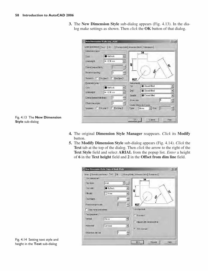
58 Introduction to AutoCAD 2006
3. The New Dimension Style sub-dialog appears (Fig. 4.13). In the dia-log make settings as shown. Then click the OK button of that dialog.
Fig. 4.13 The New DimensionStyle sub-dialog
4. The original Dimension Style Manager reappears. Click its Modifybutton.
5. The Modify Dimension Style sub-dialog appears (Fig. 4.14). Click theText tab at the top of the dialog. Then click the arrow to the right of theText Style field and select ARIAL from the popup list. Enter a heightof 6 in the Text height field and 2 in the Offset from dim line field.
Fig. 4.14 Setting text style andheight in the Text sub-dialog

Zoom, Pan and templates 59
6. Then click the Primary Units tab and set the units’ Precision in both,Linear and Angular Dimensions to 0, that is, no units after decimalpoint. Click the sub-dialog’s OK button (Fig. 4.15). The DimensionStyle Manager, dialog reappears showing dimensions, as they willappear in a drawing, in the Preview of my_style box. Click the SetCurrent button, followed by another click on the Close button.
Fig. 4.16 The right-click menu
Fig. 4.15 Setting units in thePrimary Units sub-dialog
Fig. 4.17 The Layer PropertiesManager tool icon in the Layerstoolbar
The SHORTCUTMENU variable
Call the line tool, draw a few lines and then right-click. The right-clickmenu shown in Fig. 4.16 may well appear. The menu may also appearwhen any tool is called. Some operators prefer using this menu when con-structing drawings. To stop this menu from appearing:
Command: enter shortcutmenu right-clickEnter new value for SHORTCUTMENU �12�: 0Command:
And the menu will no longer appear when a tool is in action.
Setting Layers (see also page 108)
1. Left-click on the Layer Properties Manager tool icon in the Layerstoolbar (Fig. 4.17). The Layer Properties Manager dialog appears onscreen (Fig. 4.18).
2. Click the New Layer icon. A new layer appears. Over the nameLayer1 enter Centre.
3. Repeat step 2 four times and make four more layers titled Construc-tion, Dimensions, Hidden and Text.

60 Introduction to AutoCAD 2006
4. Click against one of the squares under the Color column of the dialog.The Select Color dialog appears (Fig. 4.19). Double-click on one ofthe colours in the Index Color squares. The selected colour appearsagainst the layer name in which the square was selected. Repeat untilall five new layers have a colour.
Fig. 4.18 The Layer PropertiesManager dialog
Fig. 4.19 The Select Colordialog
5. Click on the name Continuous against the layer name Centre. TheSelect Linetype dialog appears. Click its Load . . . button and from theLoad or Reload Linetypes dialog double-click CENTER2. The dialogdisappears and the name appears in the Select Linetype dialog. Click theOK button and the linetype CENTER2 appears against the layer Centre.
6. Repeat against layer Hidden to load the linetype HIDDEN2.
Saving the template file
1. Left-click Save As . . . in the File drop-down menu.2. In the Save Drawing As dialog which comes on screen (Fig. 4.20),
click the arrow to the right of the Files of type field and in the popuplist associated with the field click on AutoCAD Drawing Template(*.dwt). The list of template files in the AutoCAD 2006/Templatedirectory appears in the file list.

Zoom, Pan and templates 61
Fig. 4.20 Saving the template tothe name acadiso.dwt
3. Click on acadiso in the file list, followed by a click on the Save button.4. A Template Description dialog appears. Make entries as indicated in
Fig. 4.21, making sure that Metric is chosen from the popup list.
Fig. 4.21 The TemplateDescription dialog
The template can now be saved and can be opened for the construction ofdrawings as needed. When AutoCAD 2006 is opened the templateacadiso.dwt fills the drawing area.
Note
Please remember that if others are using the computer, it is advisable tosave the template to a name of your own choice.
Another template
A template A4_template.dwt (Fig. 4.24)
In the Select Template dialog a click on any of the file names, causes apreview of the template to appear in the Preview box of the dialog, unlessthe template is free of information as in acadiso.dwt. To construct anothertemplate based on the acadiso.dwt template which includes a title blockand other information:

62 Introduction to AutoCAD 2006
Fig. 4.24 The A4_template.dwt
Fig. 4.23 Turn layer Vports off
Fig. 4.22 The Set Current iconin the Layer PropertiesManager
1. From the Select Template dialog select the template just completed.2. Make a new layer Vports of colour Green. Make this layer current
with a click on the Set Current icon (Fig. 4.22).3. Click the Layout1 tab below the AutoCAD drawing area. The screen is
now in a Paper Space setting.4. Click the arrow at the right of the Layers field and in the popup list
showing the layers which appears, click the Turn a layer On or Officon against the layer name Vports (Fig. 4.23).
5. Construct the border lines as shown in Fig. 4.24. To add the text enterdt (Dynamic Text) at the command line and follow the prompts whichappear in the command window.
6. It is suggested this template be saved as a Paper Space template withthe name A3_template.dwt.

Zoom, Pan and templates 63
Notes
1. The outline for this template is a pline from 0,290 to 420,290 to 420,0to 0,0 to 290,0 and of width 0.5.
2. The upper line of the title block is a pline from 0,20 to 420,20.3. The template was saved as a Paper Space file and maximised to fill
the drawing area with a click on the Maximize button in the status bar,followed by a Zoom Extents.
4. Drawings cannot be constructed in this template (it being a Pspacefile), unless the MODEL button in the status bar is ON.
5. Pspace is two-dimensional.6. Further uses for Layouts and Pspace are given in Chapter 20.
Revision notes
1. The Zoom tools are important in that they allow even the smallest partsof drawings to be examined and, if necessary, amended or modified.
2. The zoom tools can be called from icons in the Standard or Zoomtoolbars, or by entering z or zoom at the command line. The easiest isto enter z at the command line followed by a right-click.
3. There are four methods of calling tools for use – selecting a tool iconfrom a toolbar; entering the name of a tool in full at the command line;entering an abbreviation for a tool; selecting from a drop-down menu.
4. When constructing large drawings, the Pan tool and the Aerial Viewwindow are of value for allowing work to be carried out in any part of adrawing, while showing the whole drawing in the Aerial View window.
5. An A3 sheet of paper is 420 mm by 297 mm. If a drawing constructedin the template acadiso.dwt is printed/plotted full size (scale 1:1), eachunit in the drawing will be 1 mm in the print/plot.
6. When limits are set it is essential to call Zoom followed by a (All) toensure that the limits of the drawing area are as set.
7. If the right-click menu appears when using tools, the menu can beaborted by setting the SHORTCUTMENU variable to 0.

64
CHAPTER 5
The Modify tools
Aim of this chapter
To describe the uses of tools from the Modify toolbar.
Introduction
The Modify tools are among the most frequently used tools of AutoCAD2006. Drag the Modify toolbar (Fig. 5.1) from its usual position into thedrawing area.
Fig. 5.1 The Modify toolbar
Fig. 5.3 First example – Copy –outlines
Fig. 5.2 The Copy tool icon fromthe Modify toolbar
25
25
200
130
55
The Erase tool was described in Chapter 2. Examples of the othertools other than the Explode follow. See Chapter 9 for Explode.
The Copy tool
First example – Copy (Fig. 5.4)
1. Construct Fig. 5.3 using Polyline. Do not include the dimensions.2. Call the Copy tool – either left-click on its tool icon in the Modify
toolbar (Fig. 5.2), or pick Copy from the Modify drop-down menu, orenter cp or copy at the command line. The command line shows:

The Modify tools 65
Command:_copySelect objects: pick the cross 1 foundSelect objects: right-clickSpecify base point or displacement: end of pickSpecify second point of displacement or �use first point as
displacement�: pickSpecify second point of displacement: right-clickCommand:
First example – Multiple copy (Fig. 5.5)
1. Erase the copied object.2. Call the Copy tool. The command line shows:
Command:_copySelect objects: pick 1 foundSelect objects: right-clickSpecify base point or displacement:Specify base point: pickSpecify second point of displacement: pickSpecify second point of displacement or �use first point as dis-
placement�: pickSpecify second point of displacement: pickSpecify second point of displacement: right-clickCommand:
The result is shown in Fig. 5.5.
Fig. 5.4 First example – Copy
base pointsecond point
second point
base point
Fig. 5.5 First example – Copy –Multiple

66 Introduction to AutoCAD 2006
The Mirror tool
First example – Mirror (Fig. 5.8)
1. Construct the outline in Fig. 5.7 using Line and Arc.2. Call the Mirror tool – either left-click on its tool icon in the Modify
toolbar (Fig. 5.6), or pick Mirror from the Modify drop-down menu,or enter mi or mirror at the command line. The command lineshows:
Command:_mirrorSelect objects: pick first corner Specify opposite corner: pick 7 foundSelect objects: right-clickSpecify first point of mirror line: end of pickSpecify second point of mirror line: end of pickDelete source objects [Yes/No] �N�: right-clickCommand:
The result is shown in Fig. 5.8.
Fig. 5.6 The Mirror tool iconfrom the Modify toolbar
Fig. 5.7 First example –Mirror – outline
Fig. 5.8 First example – Mirror
30
2035
7520
35
R35
R55
R35
first corner
opposite corner
first point ofmirror line
second point of mirror line
Result ofthe mirroroperation
Second example – Mirror (Fig. 5.9)
1. Construct the outline shown in the dimensioned polyline inFig. 5.9.
2. Call Mirror and using the tool three times complete the given outline.The two points shown in Fig. 5.9 are to mirror the right-hand side ofthe outline.

The Modify tools 67
Third example – Mirror (Fig. 5.10)
If text is involved when using the Mirror tool, the set variable MIRRTEXTmust be set correctly. To set the variable:
Command: mirrtextEnter new value for MIRRTEXT �1�: 0Command:
If set to 0, text will mirror without distortion. If set to 1, text will readbackwards as indicated in Fig. 5.10.
The Offset tool
Example – Offset (Fig. 5.13)
1. Construct the four outlines shown in Fig. 5.12.2. Call the Offset tool – either left-click its tool icon in the Modify
toolbar (Fig. 5.11), or pick the tool name in the Modify drop-downmenu, or enter o or offset at the command line. The command lineshows:
Command:_offsetSpecify offset distance or [Through]: 10Select object to offset or �exit�: pick drawing 1Specify point on side to offset: pick inside the rectangleSelect object to offset or �exit�: right-clickCommand:
3. Repeat for drawings 2, 3 and 4 in Fig. 5.12 as shown in Fig. 5.13.
Fig. 5.9 Second example –Mirror
15
30 100 30
first point ofmirror line
second pointof mirror line
MIR
RT
EX
T =
1
MIR
RT
EX
T =
0
MIRRTEXT = 1
MIR
RT
EX
T =
0
Fig. 5.10 Third example – Mirror
Fig. 5.11 The Offset tool iconfrom the Modify toolbar

68 Introduction to AutoCAD 2006
The Array tool
Arrays can be in either a Rectangular form or a Polar form as shown inthe examples below.
First example – Rectangular Array (Fig. 5.17)
1. Construct the drawing in Fig. 5.14.2. Call the Array tool – either left-click the Array tool icon in the Modify
toolbar (Fig. 5.15), or pick Array . . . from the Modify drop-down menu,or enter ar or array at the command line. No matter which method isused the Array dialog appears (Fig. 5.16).
3. Make settings in the dialog:Rectangular Array radio button set on (dot in button).Row field – enter 5Column field – enter 6Row offset field – enter �50 (note the minus sign)Column offset field – enter 50
Fig. 5.12 First example – Offset –outlines
Rectangle140 × 85 of width 1 and
chamfers 15 × 15
Ellipse 135 × 70
Arc Pline of width = 1
1 2
34
40 4060
3530
35
30
110
20
20
Fig. 5.13 Example – Offset
Offset by 10Offset 3 times by 5
Offset twice by 15
Offset inside and outside
by 7.5
Ø10
40
10
10
Fig. 5.14 First example –Array – drawing to be arrayed
Fig. 5.15 The Array tool iconfrom the Modify toolbar

The Modify tools 69
4. Click the Select objects button and the dialog disappears. Window thedrawing. The dialog reappears.
5. Click the Preview� button. The dialog disappears and the arrayappears on screen with a warning dialog in the centre of the array(Fig. 5.17).
6. If satisfied click the Accept button. If not click the Modify button andmake revisions to the Array dialog fields.
Fig. 5.16 First example – theArray dialog
Fig. 5.17 First example – Array

70 Introduction to AutoCAD 2006
Second example – Polar Array (Fig. 5.21)
1. Construct the drawing in Fig. 5.18.2. Call Array. The Array dialog appears. Make settings as shown in
Fig. 5.19.
Fig. 5.18 Second example –Array – drawing to be arrayed
Ø20
1020
35
60
Fig. 5.19 Second example – thesetting in the Array dialog
3. Click the Select objects button of the dialog and window the drawing. Thedialog returns to screen. Click the Pick Center Point button (Fig. 5.20)and when the dialog disappears, pick a centre point for the array.
Fig. 5.20 Second example –Array – the Pick Center Pointbutton
Fig. 5.21 Second example – PolarArray
centre point of array
4. The dialog reappears. Click its Preview� button and when the arrayappears with its warning dialog, if satisfied with the result, click theAccept button of this dialog.

The Modify tools 71
The Move tool
Example – Move (Fig. 5.24)
1. Construct the drawing in Fig. 5.22.
Fig. 5.22 Example –Move – drawing
Fig. 5.23 The Move tool fromthe Modify toolbar
All edges are 5
Rectangle 190 × 50. Chamfers 10 × 10
2. Call Move – either click the Move tool icon in the Modify toolbar(Fig. 5.23), or pick Move from the Modify drop-down menu, or enterm or move at the command line which shows:
Command:_moveSelect objects: pick the shape in the middle of the drawingSelect objects: right-clickSpecify base point or displacement: pickSpecify second point of displacement: pickCommand:
The result is given in Fig. 5.24.
Fig. 5.24 Example – Move
Fig. 5.25 The Rotate tool iconfrom the Modify toolbar
object which has been moved
base point second point
The Rotate tool
When using the Rotate tool remember the default rotation of objectswithin AutoCAD 2006 is counterclockwise (anticlockwise).
Example – Rotate (Fig. 5.26)
1. Construct drawing 1 of Fig. 5.26 with Polyline. Copy the drawing 1three times – shown as drawings 2, 3 and 4 in Fig. 5.26.
2. Call Rotate – either left-click its tool icon in the Modify toolbar(Fig. 5.25), or pick Rotate from the Modify drop-down menu, or enter roor rotate at the command line. The command line shows:
Command:_rotateCurrent positive angle in UCS: ANGDIR � counterclockwise
ANGBASE � 0
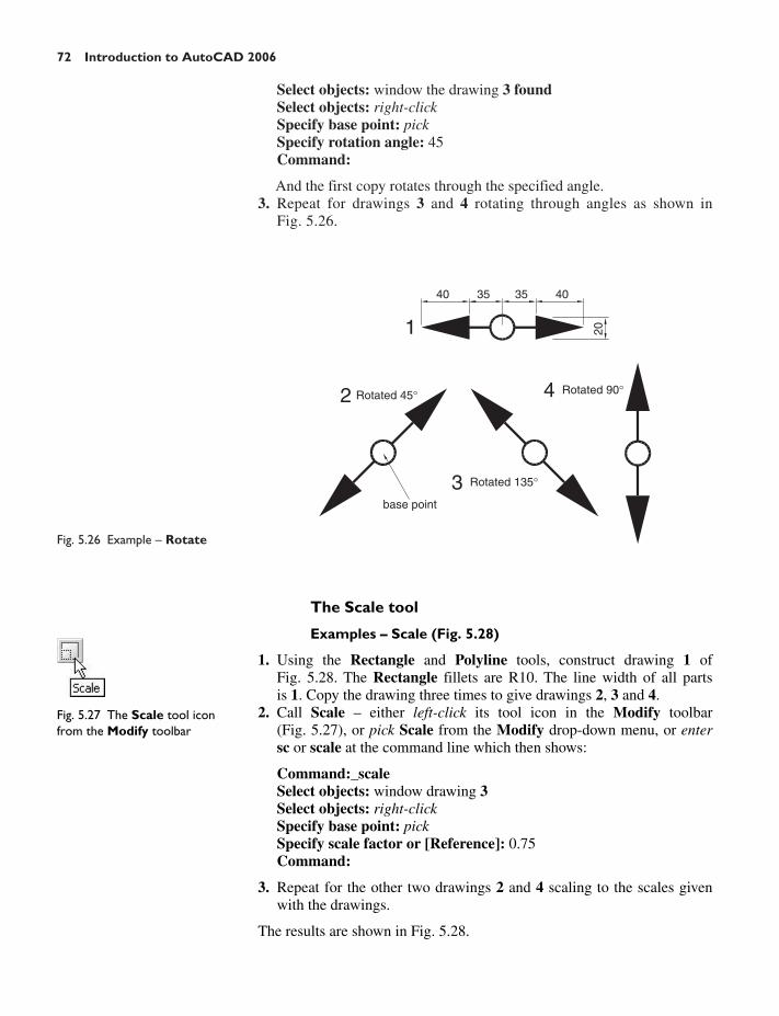
72 Introduction to AutoCAD 2006
Select objects: window the drawing 3 foundSelect objects: right-clickSpecify base point: pickSpecify rotation angle: 45Command:
And the first copy rotates through the specified angle.3. Repeat for drawings 3 and 4 rotating through angles as shown in
Fig. 5.26.
Fig. 5.26 Example – Rotate
40353540
201
Rotated 45°
Rotated 135°
Rotated 90°2
3
4
base point
Fig. 5.27 The Scale tool iconfrom the Modify toolbar
The Scale tool
Examples – Scale (Fig. 5.28)
1. Using the Rectangle and Polyline tools, construct drawing 1 ofFig. 5.28. The Rectangle fillets are R10. The line width of all partsis 1. Copy the drawing three times to give drawings 2, 3 and 4.
2. Call Scale – either left-click its tool icon in the Modify toolbar(Fig. 5.27), or pick Scale from the Modify drop-down menu, or entersc or scale at the command line which then shows:
Command:_scaleSelect objects: window drawing 3Select objects: right-clickSpecify base point: pickSpecify scale factor or [Reference]: 0.75Command:
3. Repeat for the other two drawings 2 and 4 scaling to the scales givenwith the drawings.
The results are shown in Fig. 5.28.

The Modify tools 73
The Trim tool
This tool is one which will be frequently used for the construction ofdrawings.
First example – Trim (Fig. 5.30)
1. Construct the drawing labelled Original drawing in Fig. 5.30 withCircle and Line.
2. Call Trim – either left-click its tool icon in the Modify toolbar(Fig. 5.29), or pick Trim from the Modify drop-down menu, or enter tror trim at the command line, which then shows:
Command:_trimCurrent settings: Projection UCS. Edge�NoneSelect cutting edges: pick the left-hand circle 1 foundSelect objects: right-clickSelect objects to trim or shift-select to extend or [Project/Edge/
Undo]: pick one of the objectsSelect objects to trim or shift-select to extend or [Project/Edge/
Undo]: pick the second of the objectsSelect objects to trim or shift-select to extend or [Project/Edge/
Undo]: right-clickCommand:
3. This completes the First stage as shown in Fig. 5.30. Repeat the Trimsequence for the Second stage.
4. The Third stage drawing of Fig. 5.30 shows the result of the trims atthe left-hand end of the drawing.
5. Repeat for the right-hand end. The final result is shown in the drawinglabelled Result in Fig. 5.30.
Second example – Trim (Fig. 5.31)
1. Construct the left-hand drawing of Fig. 5.31.2. Call Trim. The command line shows:
Command:_trimCurrent settings: Projection UCS. Edge�None
Fig. 5.28 Examples – Rotate
SQ35 80 20
35151 2
34
Scaled 0.75
Scaled 1.5
Scaled 1.75
base point
Fig. 5.29 The Trim tool iconfrom the Modify toolbar

74 Introduction to AutoCAD 2006
Fig. 5.31 Second example – Trim
100
12080
objects to trim
cutting edgesResult
Fig. 5.30 First example – Trim
First stage Second stage Third stage
R20R15
100
20
R15R10
Original drawing
Result
cutting edgesobjects to trim
cutting edges
Select cutting edges: pick the left-hand arc 1 foundSelect objects: right-clickSelect objects to trim or shift-select to extend or [Project/Edge/
Undo]: e (Edge)Enter an implied edge extension mode [Extend/No extend] �No
extend�: e (Extend)Select objects to trim: pickSelect objects to trim: pickSelect objects to trim: right-clickCommand:
3. Repeat for the other required trims. The result is given in Fig. 5.31.

The Stretch tool
Examples – Stretch (Fig. 5.33)
As its name implies the Stretch tool is for stretching drawings or parts ofdrawings. The action of the tool prevents it from altering the shape ofcircles in any way. Only crossing or polygonal windows can be used todetermine the part of a drawing which is to be stretched.
1. Construct the drawing labelled Original in Fig. 5.33, but do notinclude the dimensions. Use the Circle, Arc, Trim and Polyline Edittools. The resulting outlines are plines of width � 1. With the Copytool make two copies of the drawing.
Note
In each of the three examples in Fig. 5.33, the broken lines representthe crossing windows required when Stretch is used.
2. Call the Stretch tool – either click on its tool icon in the Modify tool-bar (Fig. 5.32), or pick its name in the Modify drop-down menu, orenter s or stretch at the command line which shows:
Command:_stretchSelect objects to stretch by crossing-window or crossing-polygon.Select objects: enter c right-clickSpecify first corner: pick Specify opposite corner: pick 1 foundSelect objects: right-clickSpecify base point or displacement: pick beginning of arrowSpecify second point of displacement or �use first point as displace-
ment�: drag in the direction of the arrow to the required secondpoint and right-click
Command:
The Modify tools 75
Fig. 5.32 The Stretch tool iconfrom the Modify toolbar
Fig. 5.33 Examples – Stretch
Original
First example
Second example
Thirdexample
pick corner
opposite corner
5
155
R20120
R10
R11
5

Notes
1. When circles are windowed with the crossing-window no stretching cantake place. This is why, in the case of the first example in Fig. 5.33,when the second point of displacement was picked, there was noresult – the outline did not stretch.
2. Care must be taken when using this tool as unwanted stretching can occur.
The Break tool
Examples – Break (Fig. 5.35)
1. Construct the rectangle, arc and circle (Fig. 5.35).2. Call Break – either click its tool icon in the Modify toolbar (Fig. 5.34),
or click Break from the Modify drop-down menu, or enter br or breakat the command line which shows:
For drawings 1 and 2
Command:_break Select object: pick at the pointSpecify second break point or [First point]: pickCommand:
For drawing 3
Command:_break Select object: pick at the pointSpecify second break point or [First point]: enter f right-clickSpecify first break point: pickSpecify second break point: pickCommand:
The results are shown in Fig. 5.35.
76 Introduction to AutoCAD 2006
Fig. 5.34 The Break tool iconfrom the Modify toolbar
Fig. 5.35 Examples – Break
Select
Select
second breakpoint
Result
Result
Result
second point
first point
1
2
3

Note
Remember the default rotation of AutoCAD 2006 is counterclockwise.This applies to the use of the Break tool.
The Join tool
The Join tool can be used to join plines, providing their ends are touching,lines which are in line with each other, arcs and convert arcs to circles.
Examples – Join (Fig. 5.37)
1. Construct a rectangle from four separate plines – drawing 1 of Fig. 5.37;construct two lines – drawing 2 of Fig. 5.37 and an arc – drawing 3 ofFig. 5.37.
2. Call the Join tool – either click the Join tool icon in the Modify toolbar(Fig. 5.36) or enter join or j at the command line. The command lineshows:
Command: _ join Select source object:Select objects to join to source: pick a pline 1 foundSelect objects to join to source: pick another 1 found, 2 totalSelect objects to join to source: pick another 1 found, 3 totalSelect objects to join to source: right-click3 segments added to polylineCommand: right-clickJOIN Select source object: pick one of the linesSelect lines to join to source: pick the other 1 foundSelect lines to join to source: right-click1 line joined to sourceCommand: right-clickJOIN Select source object: pick the arcSelect arcs to join to source or [cLose]: enter l right-clickArc converted to a circle.Command:
The Modify tools 77
Fig. 5.36 The Join tool icon fromthe Modify toolbar
Fig. 5.37 Examples – Join
Result 2
Result 3Result 1
1
2
3

The Extend tool
Examples – Extend (Fig. 5.39)
1. Construct plines and a circle as shown in the left-hand drawings ofFig. 5.39.
2. Call Extend – either click the Extend tool in the Modify toolbar(Fig. 5.38), or pick Extend from the Modify drop-down menu, or enterex or extend at the command line which then shows:
Command:_extendCurrent settings: Projection�UCS Edge�ExtendSelect boundary edges: pickSelect objects: right-clickSelect object to extend or shift-select to trim or [Project/Edge/
Undo]: pickRepeat for each object to be extended. Then:Select object to extend or shift-select to trim or [Project/Edge/
Undo]: right-clickCommand:
78 Introduction to AutoCAD 2006
Fig. 5.38 The Extend tool iconfrom the Modify toolbar
Fig. 5.39 Examples – Extend
Resultsboundary edge
objects toextend
objects toextend
Note
Observe the similarity of the Extend and No extend prompts with thoseof the Trim tool.
The Chamfer and Fillet tools
There are similarities in the prompt sequences for these two tools. The majordifferences are that two settings (Dist1 and Dist2) are required for a chamfer,but only one (Radius) for the fillet. The basic prompts for both are:
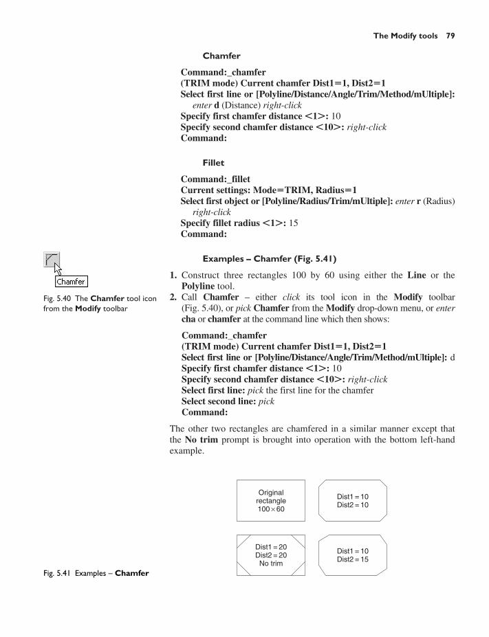
Chamfer
Command:_chamfer(TRIM mode) Current chamfer Dist1�1, Dist2�1Select first line or [Polyline/Distance/Angle/Trim/Method/mUltiple]:
enter d (Distance) right-clickSpecify first chamfer distance �1�: 10Specify second chamfer distance �10�: right-clickCommand:
Fillet
Command:_filletCurrent settings: Mode�TRIM, Radius�1Select first object or [Polyline/Radius/Trim/mUltiple]: enter r (Radius)
right-clickSpecify fillet radius �1�: 15Command:
Examples – Chamfer (Fig. 5.41)
1. Construct three rectangles 100 by 60 using either the Line or thePolyline tool.
2. Call Chamfer – either click its tool icon in the Modify toolbar(Fig. 5.40), or pick Chamfer from the Modify drop-down menu, or entercha or chamfer at the command line which then shows:
Command:_chamfer(TRIM mode) Current chamfer Dist1�1, Dist2�1Select first line or [Polyline/Distance/Angle/Trim/Method/mUltiple]: dSpecify first chamfer distance �1�: 10Specify second chamfer distance �10�: right-clickSelect first line: pick the first line for the chamferSelect second line: pickCommand:
The other two rectangles are chamfered in a similar manner except thatthe No trim prompt is brought into operation with the bottom left-handexample.
The Modify tools 79
Fig. 5.40 The Chamfer tool iconfrom the Modify toolbar
Fig. 5.41 Examples – Chamfer
Dist1 = 10Dist2 = 10
Dist1 = 10Dist2 = 15
Dist1 = 20Dist2 = 20No trim
Originalrectangle100 × 60
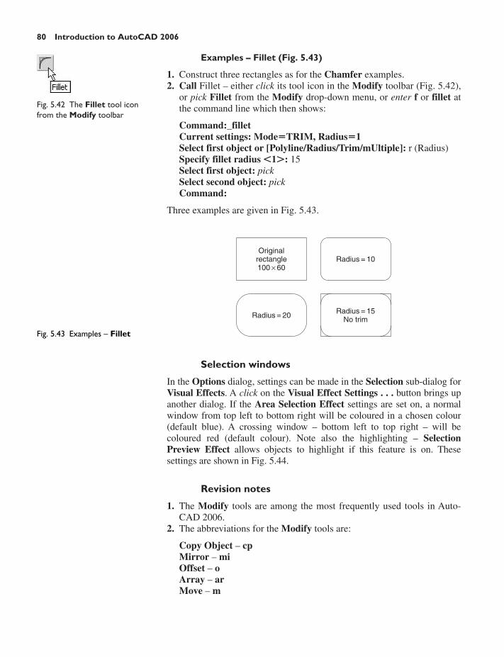
Examples – Fillet (Fig. 5.43)
1. Construct three rectangles as for the Chamfer examples.2. Call Fillet – either click its tool icon in the Modify toolbar (Fig. 5.42),
or pick Fillet from the Modify drop-down menu, or enter f or fillet atthe command line which then shows:
Command:_filletCurrent settings: Mode�TRIM, Radius�1Select first object or [Polyline/Radius/Trim/mUltiple]: r (Radius)Specify fillet radius �1�: 15Select first object: pickSelect second object: pickCommand:
Three examples are given in Fig. 5.43.
80 Introduction to AutoCAD 2006
Selection windows
In the Options dialog, settings can be made in the Selection sub-dialog forVisual Effects. A click on the Visual Effect Settings . . . button brings upanother dialog. If the Area Selection Effect settings are set on, a normalwindow from top left to bottom right will be coloured in a chosen colour(default blue). A crossing window – bottom left to top right – will becoloured red (default colour). Note also the highlighting – SelectionPreview Effect allows objects to highlight if this feature is on. Thesesettings are shown in Fig. 5.44.
Revision notes
1. The Modify tools are among the most frequently used tools in Auto-CAD 2006.
2. The abbreviations for the Modify tools are:
Copy Object – cpMirror – miOffset – oArray – arMove – m
Fig. 5.42 The Fillet tool iconfrom the Modify toolbar
Fig. 5.43 Examples – Fillet
Originalrectangle100 × 60
Radius = 10
Radius = 20 Radius = 15No trim

The Modify tools 81
Fig. 5.44 Visual Setting Effectssettings in the Options dialog
Rotate – roScale – scStretch – sTrim – trExtend – exBreak – brChamfer – chaFillet – f
3. There are two other tools in the Modify toolbar: Erase – some exampleswere given in Chapter 2; and Explode – further details of this tool will begiven in Chapter 9.
4. When using Mirror, if text is part of the area to be mirrored, the setvariable MIRRTEXT will require setting – to either 1 or 0.
5. With Offset the Through prompt can be answered by clickingtwo points in the drawing area – the distance of the desired offsetdistance.
6. Polar Arrays can be arrays around any angle set in the Angle ofarray field of the Array dialog.
7. When using Scale, it is advisable to practise the Reference prompt.8. The Trim tool in either its Trim or its No trim modes is among the
most useful tools in AutoCAD 2006.9. When using Stretch, circles are unaffected by the stretching.
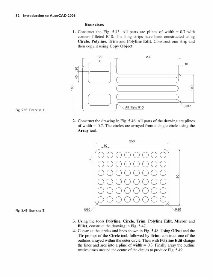
82 Introduction to AutoCAD 2006
Exercises
1. Construct the Fig. 5.45. All parts are plines of width � 0.7 withcorners filleted R10. The long strips have been constructed usingCircle, Polyline, Trim and Polyline Edit. Construct one strip andthen copy it using Copy Object.
Fig. 5.45 Exercise 1
160
2040
23012080
10
100
R10All fillets R10
Fig. 5.46 Exercise 2
25030
30
Ø20 R20
190
2. Construct the drawing in Fig. 5.46. All parts of the drawing are plinesof width � 0.7. The circles are arrayed from a single circle using theArray tool.
3. Using the tools Polyline, Circle, Trim, Polyline Edit, Mirror andFillet, construct the drawing in Fig. 5.47.
4. Construct the circles and lines shown in Fig. 5.48. Using Offset and theTtr prompt of the Circle tool, followed by Trim, construct one of theoutlines arrayed within the outer circle. Then with Polyline Edit changethe lines and arcs into a pline of width � 0.3. Finally array the outlinetwelve times around the centre of the circles to produce Fig. 5.49.

The Modify tools 83
Fig. 5.49 Exercise 4
R5
R10
Offset 5
Fig. 5.47 Exercise 3
Fig. 5.48 Exercise 4 – circlesand lines on which the exerciseis based
3010R20
R20
260160
R20
R15
10
Ø50
Ø80
30°
Ø200
Ø220

84 Introduction to AutoCAD 2006
5. Construct the arrow (Fig. 5.50). Array the arrow around the centreof its circle eight times to produce the right-hand drawing ofFig. 5.50.
Fig. 5.50 Exercise 5
20
30
10
80
R15
∅20
6. Construct the left-hand drawing of Fig. 5.51. Then with Move,move the central outline to the top left-hand corner of theouter outline. Then with Copy Object make copies to the othercorners.
Fig. 5.51 Exercise 6
170
100
R7.5
30
10
Chamfers 20 × 10
7. Construct the drawing in Fig. 5.52 and make two copies usingCopy Object. With Rotate rotate each of the copies to the anglesas shown.
8. Construct the dimensioned drawing of Fig. 5.53. With CopyObject copy the drawing. Then with Scale scale the originaldrawing to a scale of 0.5, followed by Rotate to rotate thedrawing through the angle as shown. Finally scale the copy to ascale of 2:1.
9. Construct the left-hand drawing of Fig. 5.54. Include the dimensionsin your drawing. Then, using the Stretch tool, stretch the drawing,

The Modify tools 85
Fig. 5.54 Exercise 9
12
17511590
150
100
14011
070
Fig. 5.52 Exercise 7
R20
20
R10
R20Ø30
130
30Ø30
Rotated 330° Rotated 315°
Fig. 5.53 Exercise 8
R2090
35
R20
Ø60Ø30
20Rotate 300°
Scale 2
15
Scale 0.5
including its dimensions to the sizes as shown in the right-handdrawing. Note that the dimensions change as the drawing is stretched.The dimensions are said to be associative (See Chapter 6).

10. Construct the drawing in Fig. 5.55. All parts of the drawing are plinesof width � 0.7. The setting in the Array dialog is to be 180 in theAngle of array field.
86 Introduction to AutoCAD 2006
Fig. 5.55 Exercise 10
Polar Array16 times inangle 180°
R90
R10
10

87
CHAPTER 6
Dimensions and Text
Aims of this chapter
1. To describe the variety of methods of dimensioning drawings.2. To describe methods of adding text to drawings.
Introduction
We have already set a dimension style (my_style) in the acadiso.dwttemplate, so we can now commence adding dimensions to drawings usingthis dimension style. This style name appears in the Styles toolbarbecause AutoCAD 2006 opens with the acadiso.dwt template.
The Dimension tools
Right-click in any toolbar on screen and select Dimension from the menuwhich appears. The toolbar appears (Fig. 6.1). Two tooltips are shown –Linear and Dimension Style. Click on the icon of the latter and theDimension Style Manager appears. Note the name of the dimensionstyle (my_style) that appears in the toolbar. If several dimension styleshave been saved, a popup list from the field showing all style names willappear allowing a choice of style to be made.
Fig. 6.1 The Dimension toolbar
Adding dimensions using the tools
First example – Linear Dimension (Fig. 6.2)
1. Construct a rectangle 180 � 110 using the Polyline tool.2. Left-click on the Linear tool icon in the Dimension toolbar (Fig. 6.1).
The command line shows:
Command:_dimlinearSpecify first extension line origin or [select object]: pick

Specify second extension line origin: pickSpecify dimension line location or [Mtext/Text/Angle/Horizontal/
Vertical/Rotated]: pickDimension text � 180Command:
Fig. 6.2 shows the 180 dimension. Follow exactly the same procedure forthe 110 dimension.
88 Introduction to AutoCAD 2006
Fig. 6.2 First example – LinearDimension
180
110
firstextensionline
second extensionline
dimension line location
Notes
1. If necessary use Osnaps to locate the extension line locations.2. The prompt Specify first extension line origin or [select object]:
allows the line being dimensioned to be selected.
Second example – Aligned Dimension (Fig. 6.4)
1. Construct the outline in Fig. 6.4 using the Line tool.2. Left-click the Aligned tool icon (Fig. 6.3) and dimension the out-
line. The prompts and replies are similar to the first example.
Fig. 6.3 The Aligned tool icon inthe Dimension toolbar
Fig. 6.4 Second example –Aligned Dimension
170
99
50
170
139

Third example – Radius Dimension (Fig. 6.6)
1. Construct the outline in Fig. 6.6 using the Line and Fillet tools.2. Left-click the Radius tool icon in the Dimension toolbar (Fig. 6.5).
The command line shows:
Command:_dimradiusSelect arc or circle: pick one of the arcsDimension text � 30Specify dimension line location or [Mtext/Text/Angle]: pickCommand:
3. Continue dimensioning the outline as shown in Fig. 6.6.
Dimensions and Text 89
Fig. 6.5 The Radius tool fromthe Dimension toolbar
Fig. 6.6 Third example – RadiusDimension
190R20
100
R30
Fig. 6.7 A radius dimension at anangle of 45°
Notes
1. At the prompt [Mtext/Text/Angle]:(a) If a t (Text) is entered, another number can be entered, but remem-
ber if the dimension is a radius the letter R must be entered as aprefix to the new number.
(b) If the response is a (Angle), and an angle number is entered, thetext for the dimension will appear at an angle. Fig. 6.7 shows aradius dimension entered at an angle of 45°.
(c) If the response is m (Mtext) the Text Formatting dialog appearstogether with a box in which new text can be entered. See page 100.
2. Dimensions added to a drawing using other tools from the toolbarshould be practised.
Adding dimensions from the command line
Fig. 6.8 shows all the tooltips for the tools in the Dimension toolbar. Notall of these have been shown in the examples above. Some operators may
Fig. 6.8 All tools in theDimension toolbar

prefer entering dimensions from the command line. This involves enter-ing abbreviations for the required dimension such as:
For Linear Dimension – hor (horizontal) or ve (vertical);For Aligned Dimension – al;For Radius Dimension – ra;For Diameter Dimension – d;For Angular Dimension – an;For Dimension Text Edit – te;For Quick Leader – l;And to exit from the dimension commands – e (Exit).
First example – hor and ve (Horizontal and Vertical) –(Fig. 6.10)
1. Construct the outline in Fig. 6.9 using the Line tool. Its dimensions areshown in Fig. 6.10.
90 Introduction to AutoCAD 2006
Fig. 6.9 First example – outlinefor dimensions
2. At the command line enter dim. The command line will show:
Command: enter dim right-clickDim: enter hor (horizontal) right-clickSpecify first extension line origin or �select object�: pickSpecify second extension line origin: pickSpecify dimension line location or [Mtext/Text/Angle]: pickEnter dimension text �50�: right-clickDim: right-clickHORIZONTALSpecify first extension line origin or �select object�: pickSpecify second extension line origin: pickSpecify dimension line location or [Mtext/Text/Angle/Horizontal/
Vertical/Rotated]: pickEnter dimension text �140�: right-clickDim: right-click
And the 50 and 140 horizontal dimensions are added to the outline.3. Continue to add the right-hand 50 dimension. Then when the com-
mand line shows:
Dim: enter ve (vertical) right-clickSpecify first extension line origin or �select object�: pick
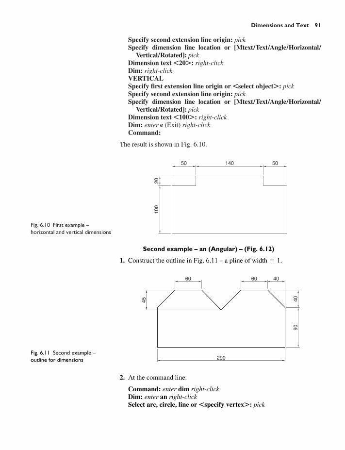
Specify second extension line origin: pickSpecify dimension line location or [Mtext/Text/Angle/Horizontal/
Vertical/Rotated]: pickDimension text �20�: right-clickDim: right-clickVERTICALSpecify first extension line origin or �select object�: pickSpecify second extension line origin: pickSpecify dimension line location or [Mtext/Text/Angle/Horizontal/
Vertical/Rotated]: pickDimension text �100�: right-clickDim: enter e (Exit) right-clickCommand:
The result is shown in Fig. 6.10.
Dimensions and Text 91
Fig. 6.10 First example –horizontal and vertical dimensions
4090
406060
290
45
Fig. 6.11 Second example –outline for dimensions
100
205014050
Second example – an (Angular) – (Fig. 6.12)
1. Construct the outline in Fig. 6.11 – a pline of width � 1.
2. At the command line:
Command: enter dim right-clickDim: enter an right-clickSelect arc, circle, line or �specify vertex�: pick

Select second line: pickSpecify dimension arc line location or [Mtext/Text/Angle]: pickEnter dimension �90�: right-clickEnter text location (or press ENTER): pickDim:
And so on to add the other angular dimensions.The result is given in Fig. 6.12.
92 Introduction to AutoCAD 2006
Fig. 6.12 Second example – andimension
Fig. 6.13 Third example – outlinefor dimensioning
20 125 1010
4515
1530
3020
70
Third example – l (Leader) – (Fig. 6.14)
1. Construct Fig. 6.13.2. At the command line:
Command: enter dim right-clickDim: enter l (Leader) right-clickLeader start: enter nea (osnap nearest) right-click to pick one of the
chamfer linesTo point: pickTo point: pickTo point: right-clickDimension text �0�: enter CHA 10�10 right-clickDim: right-click
Continue to add the other leader dimensions (Fig. 6.14).
90
6060
290
90°
Select line Select second line
135°135°

Fourth example – te (Dimension Text Edit) – (Fig. 6.16)
1. Construct Fig. 6.15.2. At the command line:
Command: enter dim right-clickDim: enter te (tedit) right-clickSelect dimension: pick the dimension to be changedSpecify new location for text or [Left/Right/Center/Home/Angle]:
either pick or enter a prompt’s capital letterDim:
Dimensions and Text 93
Fig. 6.14 Third example – Idimensions
125
4570
CHA 20 × 20
CHA 30 × 30
CHA 10 × 10
CHA 15 × 15
Fig. 6.15 Fourth example –dimensioned drawing
20 2030210
Ellipse 30 × 2030
130
2020
Ø20
Polygon
The results as given in Fig. 6.16 show dimensions which have beenmoved. The 210 dimension changed to the left-hand end of the dimension
Fig. 6.16 Fourth example –dimensions amended with tedit
20 2030210
Ellipse 30 × 20
3013
020
20
Ø20
Polygon
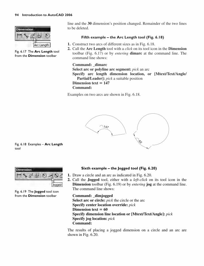
line and the 30 dimension’s position changed. Remainder of the two linesto be deleted.
Fifth example – the Arc Length tool (Fig. 6.18)
1. Construct two arcs of different sizes as in Fig. 6.18.2. Call the Arc Length tool with a click on its tool icon in the Dimension
toolbar (Fig. 6.17) or by entering dimarc at the command line. Thecommand line shows:
Command: _dimarcSelect arc or polyline arc segment: pick an arcSpecify arc length dimension location, or [Mtext/Text/Angle/
Partial/Leader]: pick a suitable positionDimension text � 147Command:
Examples on two arcs are shown in Fig. 6.18.
94 Introduction to AutoCAD 2006
Fig. 6.17 The Arc Length toolfrom the Dimension toolbar
147
62
Fig. 6.18 Examples – Arc Lengthtool
Sixth example – the Jogged tool (Fig. 6.20)
1. Draw a circle and an arc as indicated in Fig. 6.20.2. Call the Jogged tool, either with a left-click on its tool icon in the
Dimension toolbar (Fig. 6.19) or by entering jog at the command line.The command line shows:
Command: _dimjoggedSelect arc or circle: pick the circle or the arcSpecify center location override: pickDimension text � 60Specify dimension line location or [Mtext/Text/Angle]: pickSpecify jog location: pickCommand:
The results of placing a jogged dimension on a circle and an arc areshown in Fig. 6.20.
Fig. 6.19 The Jogged tool iconfrom the Dimension toolbar

Dimensions and Text 95
R60R49
Fig. 6.20 Examples – the Joggedtool
Dimension tolerances
Before simple tolerances can be included with dimensions, new set-tings will need to be made in the Dimension Style Manager dialog asfollows:
1. Open the dialog. The quickest way of doing this is to enter d at thecommand line followed by a right-click. This opens up the dialog.
2. Click the Modify . . . button of the dialog, followed by a left-clickon the Primary Units tab and in the resulting sub-dialog make set-tings as shown in Fig. 6.21. Note the changes in the preview box ofthe dialog.
Fig. 6.21 The Primary Unitssub-dialog of the DimensionStyle Manager
3. Click the Tolerances tab and in the resulting sub-dialog, make settingsas shown in Fig. 6.22. Left-click the OK button, then in the maindialog, click the Set Current button, followed by a left-click on theClose button.

96 Introduction to AutoCAD 2006
Fig. 6.22 The Tolerancessub-dialog of the DimensionStyle manager
Fig. 6.23 Example – Simpletolerances – outline
Fig. 6.24 Example – Simpletolerances – Dynamic Text The dimensions in this drawing show tolerances
65.00+0.05–0.05
∅40.00+0.05–0.05
55.00+0.05–0.05
245.00+0.05–0.05
115.
00+
0.05
–0.0
5
Example – simple tolerances (Fig. 6.24)
1. Construct the outline in Fig. 6.23.2. Dimension the drawing using either tools from the Dimension toolbar
or by entering abbreviations at the command line. Because toleranceshave been set in the Dimension Style Manager dialog, the toleranceddimensions will automatically be added to the drawing.

Dimensions and Text 97
Example – Geometrical Tolerance (Fig. 6.30)
1. Construct the two rectangles with circles as in Fig. 6.25.2. Add dimensions to the two circles.
3. Click the Tolerance tool icon (Fig. 6.26). The Geometrical Tolerancedialog (Fig. 6.27) appears.
Fig. 6.25 Example – GeometricalTolerance – dimensions to betoleranced
R15 R10
Fig. 6.26 The Tolerance toolicon in the Dimension toolbar
Fig. 6.27 The GeometricalTolerance dialog and theSymbol sub-dialog
4. In the dialog click the black box under Sym. The Symbol sub-dialog(Fig. 6.27) appears.
5. Still in the dialog click the left-hand black square under Tolerance 1.The Material Condition dialog appears (Fig. 6.28). Click L. The letterappears in the top right-hand square of the dialog.
6. Enter 0.05 in the Tolerance 1 field (Fig. 6.29), followed by a click onthe dialog’s OK button. The geometrical tolerance appears. Move it toa position near the R10 dimension in the drawing (Fig. 6.30).
7. Now add a geometrical tolerance to the R15 dimension as shown inFig. 6.30.
Fig. 6.28 The MaterialCondition dialog
Fig. 6.29 Enter 0.05 in theTolerance 1 field
Fig. 6.30 Example – Geometricaltolerances
R15 R10∅0.05 S
∅0.25 L

Text
There are two main methods of adding text to drawings – Dynamic Textand Multiline Text.
Example – Dynamic Text (Fig. 6.24)
1. Open the drawing from the example on tolerances – Fig. 6.24.2. At the command line enter dt (Dynamic Text) followed by a right-click:
Command: enter dt right-clickTEXTCurrent text style “ARIAL” Text height: 8Specify start point of text or [Justify/Style]: pickSpecify rotation angle of text �0�: right-clickEnter text: enter The dimensions in this drawing show tolerances
press the Return keyEnter text: press the Return keyCommand:
The result is given in Fig. 6.24.
Notes
1. It is essential that the Return key of the keyboard is pressed and NOTa right-click when entering text using the Dynamic Text tool.
2. At the prompt:
Specify start point of text or [Justify/Style]: enter s (Style) right-clickEnter style name or [?] �ARIAL�: enter ? right-clickEnter text style(s) to list �*�: right-click
98 Introduction to AutoCAD 2006
Fig. 6.31 The meanings of thesymbols
Straight Flat Circular Cylindrical Profile (of a line) Symmetry
PositionConcentricAngularPerpendicularParallelProfile (of a surface)
Runout (total) Runout (cicular)
The meanings of the symbols
The Material Condition letters have the following meanings:
M – maximum amount of material.L – least amount of material.S – size within the limits.
Fig. 6.31 shows the meanings of the geometrical symbols.

Dimensions and Text 99
And an AutoCAD Text Window (Fig. 6.33) appears listing all thestyles which have been selected in the Text Style (see page 57).
3. In order to select the required text style its name must be entered at theprompt:
Enter style name or [?] �ARIAL�: enter romand right-click
And the text entered will be in the Romand style of height 9. But onlyif that style was selected in the Text Style dialog.
4. Fig. 6.32 shows some text from the styles from the AutoCAD TextWindow (Fig. 6.33).
Fig. 6.32 Some text styles
Fig. 6.33 The AutoCAD TextWindow already selected in theText Style dialog
5. There are two types of text fonts available in AutoCAD 2006 – theAutoCAD SHX fonts and the Windows True Type fonts. TheITALIC, ROMAND, ROMANS and STANDARD styles shown inFig. 6.32 are AutoCAD text fonts. The TIMES and ARIAL styles areWindows True Type fonts. Most of the True Type fonts can beentered in Bold, Bold Italic, Italic or Regular styles, but these vari-ations are not possible with the AutoCAD fonts.
6. In the Font name popup list of the Text Style dialog, it will be seenthat a large number of text styles are available to the AutoCAD2006 operator. It is advisable to practise using a variety of thesefonts to familiarise oneself with the text styles available withAutoCAD 2006.

Example – Multiline Text (Fig. 6.36)
1. Open the A3_template.dwt template.2. Either left-click on the Multiline Text tool icon in the Draw toolbar
(Fig. 6.34) or enter t at the command line:
Command:_mtextCurrent text style: “ARIAL” Text height: 8Specify first corner: pickSpecify opposite corner or [Height/Justify/Line spacing/Rotation/
Style/Width]: pick
And a box such as in Fig. 6.35 appears on screen. As soon as the oppositecorner is picked, the Text Formatting dialog appears and the boxchanges as in Fig. 6.36. Text can now be entered as required within thebox as indicated in this illustration.
100 Introduction to AutoCAD 2006
Fig. 6.34 The Multiline Texttool icon from the Draw toolbar
When all the required text has been entered left-click the OK button atthe top right-hand corner of the Text Formatting dialog.
3. Changes may be made to various aspects of the text being entered,making choices from the various popup lists in the Text Formattingdialog. These popups are shown in Figs 6.37 and 6.38.
Symbols used in text
When text has to be added by entering letters and figures as part of adimension, the following symbols must be used:
To obtain Ø75 enter %%c75;To obtain 55% enter 55%%%;To obtain �0.05 enter %%p0.05;To obtain 90° enter 90%%d.
Fig. 6.35 The Multiline Text box
Fig. 6.36 Example – MultilineText entered in the text box

Dimensions and Text 101
Fig. 6.37 The popups from theText Formatting dialog
Fig. 6.38 The popup list whichappears when the Symbol icon@ is clicked
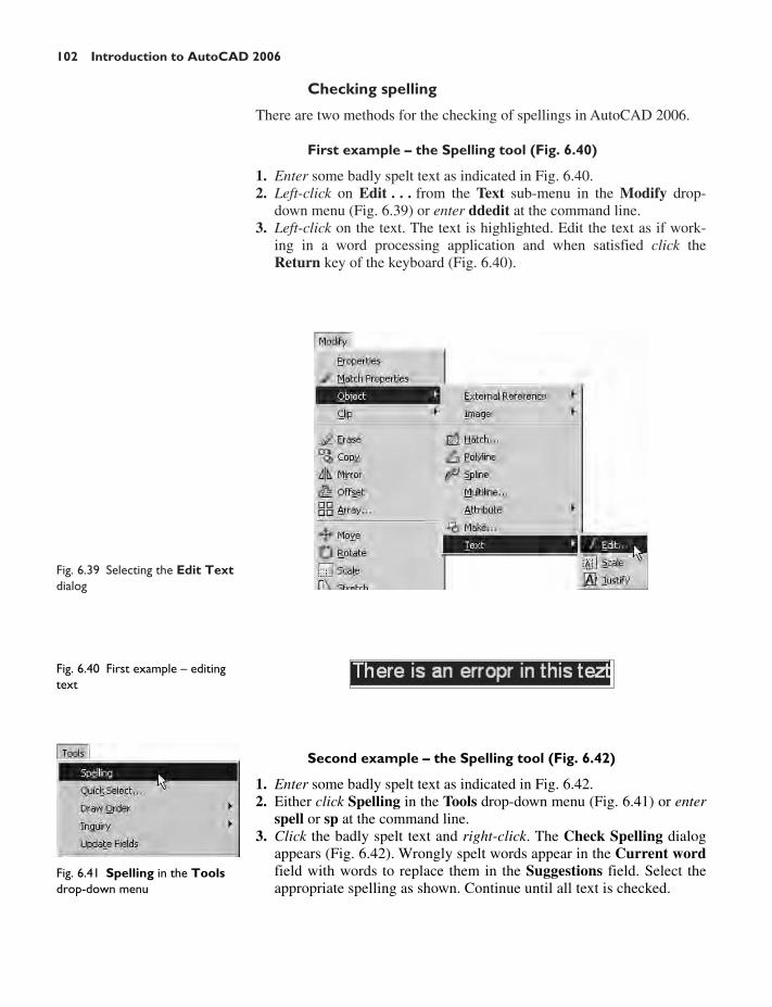
Checking spelling
There are two methods for the checking of spellings in AutoCAD 2006.
First example – the Spelling tool (Fig. 6.40)
1. Enter some badly spelt text as indicated in Fig. 6.40.2. Left-click on Edit . . . from the Text sub-menu in the Modify drop-
down menu (Fig. 6.39) or enter ddedit at the command line.3. Left-click on the text. The text is highlighted. Edit the text as if work-
ing in a word processing application and when satisfied click theReturn key of the keyboard (Fig. 6.40).
102 Introduction to AutoCAD 2006
Fig. 6.39 Selecting the Edit Textdialog
Fig. 6.40 First example – editingtext
Fig. 6.41 Spelling in the Toolsdrop-down menu
Second example – the Spelling tool (Fig. 6.42)
1. Enter some badly spelt text as indicated in Fig. 6.42.2. Either click Spelling in the Tools drop-down menu (Fig. 6.41) or enter
spell or sp at the command line.3. Click the badly spelt text and right-click. The Check Spelling dialog
appears (Fig. 6.42). Wrongly spelt words appear in the Current wordfield with words to replace them in the Suggestions field. Select theappropriate spelling as shown. Continue until all text is checked.

Dimensions and Text 103
Revision notes
1. In the Line and Arrows sub-dialog of the Dimension Style Man-ager dialog, Lineweights were set to 0.3 (page 58). If theselineweights are to show in the drawing area of AutoCAD 2006, theLWT button in the status bar must be set ON.
2. Dimensions can be added to drawings using the tools from theDimension toolbar or by entering abbreviations for the tools at thecommand line.
3. It is usually advisable to use osnaps when locating points on a draw-ing for dimensioning.
4. The Style and Angle of the text associated with dimensions can bechanged during the dimensioning process.
5. When wishing to add tolerances to dimensions it will probably be nec-essary to make new settings in the Dimension Style Manager dialog.
6. There are two methods for adding text to a drawing – Dynamic Textand Multiline Text.
7. When adding text to a drawing, the Return key must be used and notthe right-hand mouse button.
8. Text styles can be changed during the process of adding text todrawings.
9. AutoCAD 2006 uses two types of text style – AutoCAD SHX fontsand Windows True Type fonts.
Fig. 6.42 Second example – theCheck Spelling dialog

10. Most True Type fonts can be in bold, bold italic, italic or regularformat. AutoCAD fonts can only be added in the single format.
11. When using Multiline Text, changes can be made by selection fromthe popup lists in the Text Formatting dialog.
12. To obtain the symbols Ø; �; �; % use %%c; %%p; %%d; %%%respectively before or after the figures of the dimension.
13. Text spelling can be checked with by selecting Text/Edit . . . fromthe Modify drop-down menu or by entering spell at the com-mand line.
Exercises
1. Open any of the drawings previously saved from workingthrough examples or as answers to exercises and add appropriatedimensions.
2. Construct the drawing Fig. 6.43 but in place of the given dimensionsadd dimensions showing tolerances of 0.25 above and below.
104 Introduction to AutoCAD 2006
Fig. 6.43 Exercise 2
220120
R20
Chamfer 10 × 10
10
60140
25
25
Ø10
R10
3. Construct the two polygons in Fig. 6.44 and add all the diagonals. Thenset the two osnaps endpoint and intersection and using the lines as inFig. 6.44 construct the stars as shown using a polyline of width � 3.Next erase all unwanted lines. Finally dimension the angles labelled A,B, C and D.
4. Using the text style Sans Serif of height 20 and enclosing the wordingwithin a rectangle of Width � 5 and Fillet � 10, construct the drawingin Fig. 6.45.
5. Construct and dimension the drawing in Fig. 6.46.

Dimensions and Text 105
Fig. 6.44 Exercise 3 – Twopolygons
A
B
C D
8090
Fig. 6.46 Exercise 5
7070 100
3020 15
130
20
6050
5020
Ø120
Fig. 6.45 Exercise 4
AutoCAD 2006

CHAPTER 7
Orthographic and isometric
Aim of this chapter
To introduce methods of constructing drawings of two types – orthographicprojection and isometric drawings.
Orthographic projection
Orthographic projection involves viewing an article being described in atechnical drawing from different directions – from the front, from a side,from above, from below or from any other viewing position. Orthographicprojection often involves:
1. The drawing of details which are hidden, using hidden detail lines;2. Sectional views in which the article being drawn is imagined as being
cut through and the cut surface drawn;3. Centre lines through arcs, circles, spheres and cylindrical shapes.
An example of an orthographic projection
Taking the solid shown in Fig. 7.1, construct a three-view orthographicprojection of the solid:
1. Draw what is seen when the solid is viewed from its left-hand side andregard this as the front of the solid. What is drawn will be a frontview (Fig. 7.2).
2. Draw what is seen when the solid is viewed from the left-hand end ofthe front view. This produces an end view. Fig. 7.3 shows the end viewalongside the front view.
3. Draw what is seen when the solid is viewed from above the front view.This produces a plan. Fig. 7.4 shows the plan below the front view.
4. Draw centre and hidden detail lines:(a) Click the arrow to the right of the Layers field to show all layers
set in the acadiso.dwt template on which the drawing has beenconstructed (Fig. 7.5).
(b) Left-click the Centre layer name in the layers list, making it thecurrent layer. All lines will now be drawn as centre lines.
5. In the three-view drawing add centre lines.
106
Fig. 7.1 Example – orthographicprojection – the solid being drawn
60
180
3040
Ø60
Ø40
Ø120
R10
R20
110
Fig. 7.2 The front view of thesolid

Orthographic and isometric 107
6. Make the Hidden layer the current layer and add hidden detail lines.7. Make the Text layer current and add border lines and a title block.8. Make the Dimensions layer current and add all dimensions.
The completed drawing is shown in Fig. 7.6.
60
180
3040
Ø60
Ø40
Ø120
R10
R20
110
R20
Hole Ø40
R40
Fig. 7.3 Front and end views ofthe solid
60
110
R10
R20
180
∅120
∅60
∅40
3040
R40
R20
Hole ∅40
Fig. 7.4 Front and end views,and plan of the solid

108 Introduction to AutoCAD 2006
First angle and third angle
There are two types of orthographic projection – first angle and thirdangle. Fig. 7.7 is a pictorial drawing of the solid used to demonstrate thetwo angles. Fig. 7.8 shows a three-view first angle projection and Fig. 7.9shows the same views in third angle.
In both angles the viewing is from the same directions. The differenceis that the view as seen is placed on the viewing side of the front view inthird angle and on the opposite side to the viewing in first angle.
Fig. 7.5 Click the layer namecentre to make it the current layer
60
180
3040
Ø60
Ø40
Ø120
R10
R20
110
R20
Hole Ø40
R40Dimensionsin millimetres
Name: A. Student Scale: 1:1 Date: 19/07/2006 Title: PART 7/45/EB
Fig. 7.6 The completed workingdrawing of the solid
Fig. 7.7 The solid used todemonstrate first and thirdangles of projection

Orthographic and isometric 109
Sectional views
In order to show internal shapes of a solid being drawn in orthographicprojection the solid is imagined as being cut along a plane and the cut sur-face then drawn as seen. Common practice is to hatch the areas whichthen show in the cut surface. Note the section plane line, the section labeland the hatching in the sectional view Fig. 7.10.
Adding hatching
To add the hatching as shown in Fig. 7.10:
1. Call the Hatch tool – either left-click on its tool icon in the Draw tool-bar (Fig. 7.11) or enter h at the command line. Note – do not enterhatch as this gives a different result. The Hatch and Gradient dialog(Fig. 7.12) appears.
Fig. 7.9 A third angle projection
Look from thisdirection to see
a PLAN
Look from thisdirection to seean END VIEW
End view
Frontview
Plan
Fig. 7.8 A first angle projection

110 Introduction to AutoCAD 2006
2. Click in the Swatch field. The Hatch Pattern Palette appears. Left-click the ANSI tab and from the resulting pattern icons double-clickthe ANSI31 icon. The palette disappears and the ANSI31 patternappears in the Swatch field.
A A
A-A
Hatching
Section label
Section line
Fig. 7.10 A sectional view
Fig. 7.11 The Hatch tool iconfrom the Draw toolbar
Fig. 7.12 The Hatch andGradient dialog and the ANSIHatch Pattern Palette
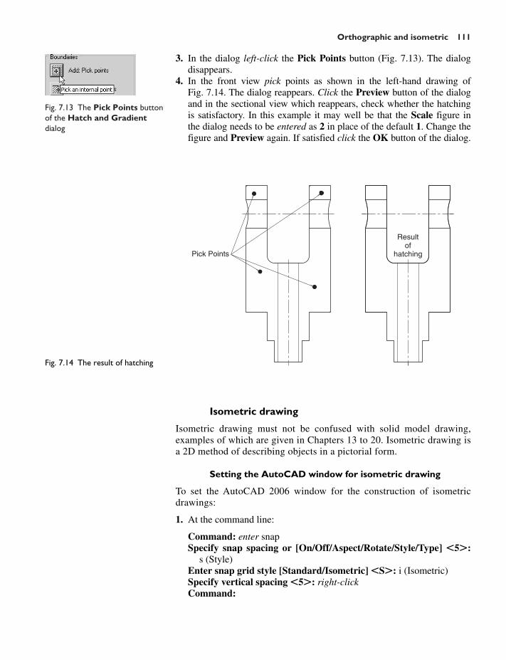
Orthographic and isometric 111
Fig. 7.13 The Pick Points buttonof the Hatch and Gradientdialog
Pick Points
Resultof
hatching
Fig. 7.14 The result of hatching
3. In the dialog left-click the Pick Points button (Fig. 7.13). The dialogdisappears.
4. In the front view pick points as shown in the left-hand drawing ofFig. 7.14. The dialog reappears. Click the Preview button of the dialogand in the sectional view which reappears, check whether the hatchingis satisfactory. In this example it may well be that the Scale figure inthe dialog needs to be entered as 2 in place of the default 1. Change thefigure and Preview again. If satisfied click the OK button of the dialog.
Isometric drawing
Isometric drawing must not be confused with solid model drawing,examples of which are given in Chapters 13 to 20. Isometric drawing isa 2D method of describing objects in a pictorial form.
Setting the AutoCAD window for isometric drawing
To set the AutoCAD 2006 window for the construction of isometricdrawings:
1. At the command line:
Command: enter snapSpecify snap spacing or [On/Off/Aspect/Rotate/Style/Type] �5�:
s (Style)Enter snap grid style [Standard/Isometric] �S�: i (Isometric)Specify vertical spacing �5�: right-clickCommand:
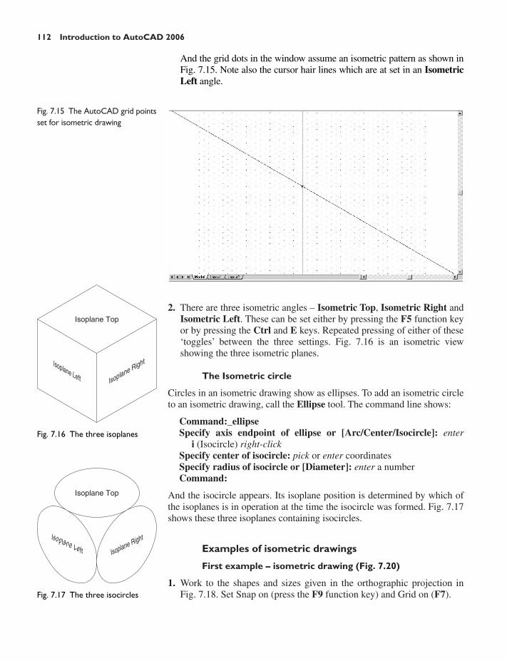
112 Introduction to AutoCAD 2006
2. There are three isometric angles – Isometric Top, Isometric Right andIsometric Left. These can be set either by pressing the F5 function keyor by pressing the Ctrl and E keys. Repeated pressing of either of these‘toggles’ between the three settings. Fig. 7.16 is an isometric viewshowing the three isometric planes.
The Isometric circle
Circles in an isometric drawing show as ellipses. To add an isometric circleto an isometric drawing, call the Ellipse tool. The command line shows:
Command:_ellipseSpecify axis endpoint of ellipse or [Arc/Center/Isocircle]: enter
i (Isocircle) right-clickSpecify center of isocircle: pick or enter coordinatesSpecify radius of isocircle or [Diameter]: enter a numberCommand:
And the isocircle appears. Its isoplane position is determined by which ofthe isoplanes is in operation at the time the isocircle was formed. Fig. 7.17shows these three isoplanes containing isocircles.
Examples of isometric drawings
First example – isometric drawing (Fig. 7.20)
1. Work to the shapes and sizes given in the orthographic projection inFig. 7.18. Set Snap on (press the F9 function key) and Grid on (F7).
Fig. 7.15 The AutoCAD grid pointsset for isometric drawing
Isoplane RightIsoplane Left
Isoplane Top
Fig. 7.16 The three isoplanes
Isoplane RightIsoplane Left
Isoplane Top
Fig. 7.17 The three isocircles
And the grid dots in the window assume an isometric pattern as shown inFig. 7.15. Note also the cursor hair lines which are at set in an IsometricLeft angle.

Orthographic and isometric 113
70
130
20
80
Ø40
Fig. 7.18 First example –isometric drawing – the model
Items 3 and 4Item 5 Item 6
Fig. 7.19 First example – isometricdrawing – items 3, 4, 5 and 6
2. Set Snap to Isometric and set the isoplane to Isoplane Top using F5.3. With Line, construct the outline of the top of the model (Fig. 7.19)
working to the dimensions given in Fig. 7.18.
4. Call Ellipse tool and set to isocircle, and add the isocircle of radius 20centred in its correct position in the outline of the top (Fig. 7.19).
5. Set the isoplane to Isoplane Right and with Copy set to Multiple, copythe top with its ellipse vertically downwards three times as shown inFig. 7.19.
6. Add lines as shown in Fig. 7.19.

114 Introduction to AutoCAD 2006
50
10
100
R15
30
Ø10
Ø20
R20
Fig. 7.21 Second example –isometric drawing – orthographicprojection of model
Fig. 7.20 First example – isometricdrawing
7. Finally using Trim remove unwanted parts of lines and ellipses toproduce Fig. 7.20.
Second example – isometric drawing (Fig. 7.22)
Fig. 7.21 is an orthographic projection of the model of which the isometricdrawing is to be constructed. Fig. 7.22 shows the stages in its construction.The numbers refer to the items in the list below.

Orthographic and isometric 115
1. In Isoplane Right construct two isocircles of radii 10 and 20.2. Add lines as in drawing 2 and trim unwanted parts of isocircle.3. With Copy copy three times as in drawing 3.4. Add lines as in drawing 4.5. In Isoplane Left add lines as in drawing 5.6. In Isoplane Right add lines and isocircles as in drawing 6.7. With Trim trim unwanted lines and parts of isocircles to complete the
isometric drawing – drawing 7.
Revision notes
1. There are, in the main, two types of orthographic projection – firstangle and third angle.
2. The number of views included in an orthographic projection depend uponthe complexity of what is being drawn – a good rule to follow is to attemptfully describing the object being drawn in as few views as possible.
3. Sectional views allow parts of an object, which are normally hiddenfrom view, to be more fully described in a projection.
4. When a layer is turned OFF, all constructions on that layer disappearfrom the screen.
5. If a layer is locked, objects can be added to the layer but no furtheradditions or modifications can be made to the layer. If an attempt ismade to modify an object on a locked layer the command line shows:
Command:_eraseSelect objects: pick 1 found1 was on a locked layer
and the object will not be modified.6. Frozen layers cannot be selected, but note that layer 0 cannot be frozen.7. Isometric drawing is a 2D pictorial method of producing illustrations
showing objects. It is not a 3D method of showing a pictorial view.8. When drawing ellipses in an isometric drawing, the Isocircle prompt
of the Ellipse tool’s command line sequence must be used.9. When constructing an isometric drawing, Snap must be set to isometric
mode before construction can commence.
1 4
2
5
3
6 7
Fig. 7.22 Second example –isometric drawing – stages in theconstruction

116 Introduction to AutoCAD 2006
Exercises
Fig. 7.23 is an isometric drawing of a slider fitment on which the threeexercises 1, 2 and 3 are based.
1. Fig. 7.24 is a first angle orthographic projection of part of the fitmentshown in the isometric drawing in Fig. 7.23. Construct a three-viewthird angle orthographic projection of the part.
R25
Ø30
5025
70
120 50
Fig. 7.25 Exercises 2 and 3
50
180
70
R10
50
R30
R5
1515
15Hole Ø30
Fig. 7.24 Exercise 1
2. Fig. 7.25 is a first angle orthographic projection of the other part of thefitment shown in Fig. 7.23. Construct a three-view third angle ortho-graphic projection of the part.
3. Construct an isometric drawing of the part shown in Fig. 7.25.
Fig. 7.23 Exercises 1, 2 and 3 – anisometric drawing of the threeparts of the slider on which theseexercises are based

Orthographic and isometric 117
Fig. 7.28 An isometric drawing ofthe angle plate on which exercises6 and 7 are based
8515
55
100
R10
R70
R5
R10
10
Fig. 7.29 Exercises 6 and 7 – anorthographic projection of theangle plate
M10
10
0
35
Ø10
5
SQ 20
Ø20
Ø10
65
25
Ø20
20
60
10
60
70
15
15
15 15
Hole Ø10
Tapped M10
Fig. 7.27 Exercises 4 and 5 –orthographic projections of thethree parts of the tool holder
Fig. 7.26 Exercises 4 and 5 – anisometric drawing of the toolholder on which the twoexercises are based
4. Construct a three-view orthographic projection, in an angle of yourown choice, of the tool holder assembled as shown in the isometricdrawing Fig. 7.26. Details are given in Fig. 7.27.
5. Construct an isometric drawing of the body of the tool holder as shownin Figs 7.26 and 7.27.
6. Construct the orthographic projection given in Fig. 7.29.7. Construct an isometric drawing of the angle plate shown in Figs 7.28
and 7.29.

118 Introduction to AutoCAD 2006
Fig. 7.30 Exercises 8 and 9 – anisometric drawing of thecomponent for the two exercises
7
1030
Holes Ø6 C'Bbore Ø1010
405
15
70 80 50 40
25 6090 85
R5035
Hole Ø12
Hole Ø14
R5
Fig. 7.31 Exercises 8 and 9
8. Construct a third angle projection of the component shown in the iso-metric drawing in Fig. 7.30 and the three-view first angle projection inFig. 7.31.
9. Construct the isometric drawing shown in Fig. 7.30 working to thedimensions given in Fig. 7.31.

119
CHAPTER 8
Hatching
Aim of this chapter
To describe further examples of the use of hatching in its various forms.
Introduction
In Chapter 7 an example of hatching a sectional view in an orthographicprojection was given. Further examples of the use of hatching will bedescribed in this chapter.
There are a large number of hatch patterns available when hatchingdrawings in AutoCAD 2006. Some examples from the Hatch PatternPalette sub-dialog from the Other Predefined set of hatch patterns(Fig. 8.2) are shown in Fig. 8.1.
Fig. 8.1 Some hatch patterns fromPredefined hatch patterns
1 2
3 4
AR-HBONEScale = 0.1
AR-BRELMScale = 0.2
AR-PARQ1Scale = 0.1
CLAYScale = 2
NET3Scale = 2
HOUNDScale = 2
5 6
Other hatch patterns can be selected form the ISO or ANSI hatch pat-tern palettes, or the operator can design their own hatch patterns and savethem to the Custom hatch palette.
First example – hatching a sectional view (Fig. 8.3)
Fig. 8.3 shows a two-view orthographic projection which includes a sec-tional end view. Note the following in the drawing:
1. The section plane line, consisting of a centre line with its ends marked Aand an arrow showing the direction of viewing to obtain the sectional view.

120 Introduction to AutoCAD 2006
2. The sectional view labelled with the letters of the section plane line.3. The cut surfaces of the sectional view hatched with the ANSI31 hatch
pattern which is generally used for the hatching of engineering draw-ing sections.
Fig. 8.2 The Other PredefinedHatch Pattern Palette
Fig. 8.3 First example –Hatching
Keyway 3 × 3
∅40∅25
R50
90
20
100
Tolerances:Linear 0.05Angular: 15° unless otherwise stated
Dimensions in mm
Name:Scale: 1:1 Date:
Title:Dwg No:
A
135
R25
25 2550R45
R25
A-A
HOLE ∅20
Materials:
DO NOT SCALE Finish:
A

Hatching 121
Second example – hatching rules (Fig. 8.4)
Fig. 8.4 describes the stages in hatching a sectional end view of a lathetool holder. Note the following in the section:
1. There are two angles of hatching to differentiate in separate parts ofthe section.
2. The section follows the general rule that parts such as screws, bolts,nuts, rivets, other cylindrical objects, webs and ribs and other such fea-tures are shown within sections as outside views.
1Pick Point
2
3 4
Pick Point
Add centre lineafter hatching
Hatch PatternANSI31 atAngle = 0 Scale = 1.5
Pick Point Pick Point
Change HatchAngle to 90
Left-click onPreview button
if satisfiedleft-click onOK button
Fig. 8.4 Second example –hatching rules for sections
Third example – Associative hatching (Fig. 8.5)
Fig. 8.5 shows two end views of a house. After constructing the left-handview, it was found that the upper window had been placed in the wrongposition. Using the Move tool, the window was moved to a new position.The brick hatching automatically adjusted to the new position. SuchAssociative hatching is only possible if the radio button against Associa-tive in the Composition area of the Hatch and Gradient dialog is ON,that is, a dot fills the radio button circle (Fig. 8.6).
Fourth example – Colour gradient hatching (Fig. 8.9)
Fig. 8.9 shows two examples of hatching from the Gradient sub-dialog ofthe Hatch and Gradient dialog.
1. Construct two outlines such as those shown in Fig. 8.9.2. Click the Gradient Hatch tool icon in the Draw toolbar (Fig. 8.7).
The Gradient sub-dialog of the Hatch and Gradient dialog appears

122 Introduction to AutoCAD 2006
frame
End view of housebefore moving
the upperwindow position
After moving framehatching adjusts
to its new
Fig. 8.5 Third example –Associative hatching
Fig. 8.6 Associative hatching seton in the Hatch and Gradientdialog
Fig. 8.7 The Gradient Hatchtool icon from the Draw toolbar
Fig. 8.8 The Gradient sub-dialogof the Hatch and Gradientdialog
(Fig. 8.8). Pick one of the gradient choices, followed with a clickon the Add Pick points button. When the dialog disappears, pick asingle area of one of the drawings, followed by a click on the dialog’sOK button when the dialog reappears.
3. Repeat in each of the other areas of the drawing.4. Change the gradient choice and repeat items 3 and 4 in the other
drawing.
The result is shown in Fig. 8.9.

Hatching 123
Fig. 8.9 Fourth example –Gradient hatching
Fig 8.10 The buttons for bringingthe Select Color dialog to screen
Fig. 8.11 The More Optionsarrow of the Hatch andGradient dialog
Notes
1. If the Two color radio button is set on (dot in circle) the coloursinvolved in the gradient hatch can be changed by clicking the buttonmarked with three (. . .) (Fig. 8.10) on the right of each of the colourfields. This brings a Select Color dialog on screen, which offers threechoices of sub-dialogs from which to select colours.
2. Sliders in the Select Color dialogs offer changes in colour shading asthe slider is moved under mouse control.
Fifth example – Advanced hatching (Fig. 8.13)
If the arrow at the bottom right-hand corner of the Hatch and Gradientdialog is clicked (Fig. 8.11) the dialog expands to show the Island Displayselections (Fig. 8.12).
1. Construct a drawing which includes three outlines as shown in the left-hand drawing of Fig. 8.13 and copy it twice to produce three identicaldrawings.
2. Select the hatch pattern HONEY at an angle of 0 and scale 1.3. Click in the Normal radio button of the Island display style area.4. Pick a point in the left-hand drawing. The drawing hatches as shown.5. Repeat in the centre drawing with the radio button of the Outer style
set on (dot in button).6. Repeat in the right-hand drawing with Ignore set on.

124 Introduction to AutoCAD 2006
Fig. 8.13 Fifth example –Advanced hatching
pick points
Normal Outer Ignore
Fig. 8.12 The Island Displayselections in the expandedHatch and Gradient dialog
Sixth example – Text in hatching (Fig. 8.14)
1. Construct a pline rectangle using the sizes given in Fig. 8.14.2. In the Text Style Manager dialog, set the text font to Arial and its
Height � 25.3. Using the Dtext tool enter the text as shown central to the rectangle.4. Hatch the area using the HONEY hatch pattern set to an angle of 0
and scale of 1.
The result is shown in Fig. 8.14.

Hatching 125
Fig. 8.16 Seventh example –construction on layer 0
Note
Text will be entered with a surrounding boundary area free from hatching,providing the Advanced Normal radio button is set on.
Seventh example – Advanced hatching (Fig. 8.20)
1. Open the Layer Properties Manager with a click on its icon in theLayer toolbar.
2. Make layers as shown in Fig. 8.15.
Fig. 8.14 Sixth example – Textin hatching
275
90 AutoCAD 2006
3. With the layer 0 current, construct the outline as given in Fig. 8.16.
Fig. 8.15 Seventh example – thelayers setup for the advancedhatch example

126 Introduction to AutoCAD 2006
Fig. 8.18 Seventh example –construction on layer Hatchboundaries
6. Make the layer HATCH current and add hatching to the areas shownin Fig. 8.19 using the hatch patterns ANGLE at scale 2 for the roofand BRICK at a scale of 0.75 for the wall.
5. With layer Hatch boundaries current, construct the lines as shown inFig. 8.18.
Fig. 8.17 Seventh example –construction on layer 1
4. With layer 1 current, construct the door and windows (Fig. 8.17).

Hatching 127
Fig. 8.20 Seventh example – thefinished drawing
7. Finally turn the layer Hatch boundaries off. The result is given inFig. 8.20.
Fig. 8.19 Seventh example –construction on layer HATCH
Revision notes
1. A large variety of hatch patterns are available when working withAutoCAD 2006.
2. In sectional views in engineering drawings it is usual to show itemssuch as bolts, screws, other cylindrical objects, webs and ribs as out-side views.

128 Introduction to AutoCAD 2006
40 45
R35
A
190
A
HOLE ∅30 ∅5035
15 2070
8550
Fig. 8.22 Exercise 1
3. When associative hatching is set on, if an object is moved within ahatched area, the hatching accomodates to fit around the movedobject.
4. Colour gradient hatching is available in AutoCAD 2006.5. When hatching takes place around text, a space around the text will be
free from hatching.
Exercises
1. Fig. 8.21 shows a pictorial drawing of the component shown in thethree-view orthographic projection in Fig. 8.22. Construct the threeviews with the front view as a sectional view based on the sectionplane A-A.
Fig. 8.21 Exercise 1 – a pictorialview
2. Construct the three-view orthographic projection in Fig. 8.23 to thegiven dimensions with the front view as the sectional view A-A.
3. Construct the drawing Stage 5 following the descriptions of stagesgiven in Fig. 8.24.
4. Fig. 8.25 is a front view of a car with parts hatched. Construct asimilar drawing of any make of car, using hatching to emphasise theshape.
5. Working to the notes given with the drawing in Fig. 8.26, construct theend view of a house as shown. Use your own discretion about sizes forthe parts of the drawing.
6. Working to dimensions of your own choice, construct the three-viewprojection of a two-storey house as shown in Fig. 8.27.

Hatching 129
Stage 1 Construct word on Layer 0 and offset on Layer 1
Stage 2 Hatch on Layer HATCH01 Hatch with SOLID
Stage 3 Turn Layer 0 off Turn HATCH01 off Add lines as shown
Stage 4 Turn HATCH02 on Hatch with ANSI31 at Angle 135 and Scale 40 Turn HATCH02 off
Stage 5 Turn Layer 0 off Turn HATCH01 onFig. 8.24 Exercise 3
Fig. 8.25 Exercise 4
4 HOLES ∅12
10
60
10
50
10
40
190
10
1075
A
A70
60 50
ROLLER ∅40
Fillets areR3, R4 and R10
Fig. 8.23 Exercise 2

130 Introduction to AutoCAD 2006
7. Construct Fig. 8.28 as follows:(a) On layer Text, construct a circle of radius 90.(b) Make layer 0 current.(c) Construct the small drawing to the details as shown and save as a
block with a block name shape (see Chapter 9).(d) Call the Divide tool by entering div at the command line:
Fig. 8.27 Exercise 6
Hatch PatternANGLE
Scale = 0.025Angle = 0
Windows are55 × 35 withbars 1 and 2
wide
Hatch PatternAE-BBB
Scale = 0.025Angle = 0
7025
5
25Hatch PatternSAND
Scale = 0.1
160 60
Hatch PatternBRICK
Scale = 0.8Angle = 0
Hatch PatternBRSTONE
Scale = 0.7Angle = 0
110
170 18
0
5
10
Hatch PatternAR-BBB
Scale = 0.4Angle = 0
Angle = 0
Fig. 8.26 Exercise 5

Hatching 131
Hatch withSTARSScale = 0.75
R70
35 40
30
Fig. 8.28 Exercise 7
Command: enter div right-clickSelect object to divide: pick the circleEnter number of segments or [Block]: enter b right-clickEnter name of block to insert: enter shape right-clickAlign block with object? [Yes/No] �Y�: right-clickEnter the number of segments: enter 20 right-clickCommand:
(e) Turn the layer Text off.

CHAPTER 9
Blocks and Inserts
Aims of this chapter
1. To describe the construction of blocks and wblocks (written blocks).2. To introduce the insertion of blocks and wblocks into other drawings.3. To introduce the use of the DesignCenter palette.4. To explain the use of Explode and Purge tools.
Introduction
Blocks are drawings which can be inserted into other drawings. Blocksare contained in the data of the drawing in which they have been con-structed. Wblocks (written blocks) are saved as drawings in their ownright, but can be inserted into other drawings if required.
Blocks
First example – Blocks (Fig. 9.3)
1. Construct the building symbols as shown in Fig. 9.1 to a scale of 1:50.
132
Garage door
2.5 m window 2 m window Main door Room door
Chair3Chair2ChairSingle bedDouble bed
Table WC Bath Shrub
Fig. 9.1 First example –Blocks – symbols to be savedas blocks
2. Left-click the Make Block tool (Fig. 9.2). The Block Definitiondialog (Fig. 9.3) appears. To make a block of the Double bed symboldrawing:

(a) Enter double bed in the Name field.(b) Click the Select Objects button. The dialog disappears. Window
the drawing of the double bed. The dialog reappears. Note the iconof the double bed in the Preview icon area of the dialog.
(c) Click the Pick Point button. The dialog disappears. Click a pointon the double bed drawing to determine its insertion point. Thedialog reappears. Note the coordinates of the insertion point,which appear in the Base point area of the dialog.
(d) If thought necessary enter a description in the Description field ofthe dialog.
The drawing is now saved as a block in the drawing.3. Repeat steps 1 and 2 to make blocks of all the other symbols in the
drawing.4. Open the Block Definition dialog again and click the arrow on the
right of the Name field. The blocks saved in the drawing appear in apopup list (Fig. 9.4).
Blocks and Inserts 133
Fig. 9.2 The Make Block toolicon from the Draw toolbar
Fig. 9.3 The Block Definitiondialog with entries for the doublebed
Fig. 9.4 The popup list in theName field showing all blockssaved in the drawing
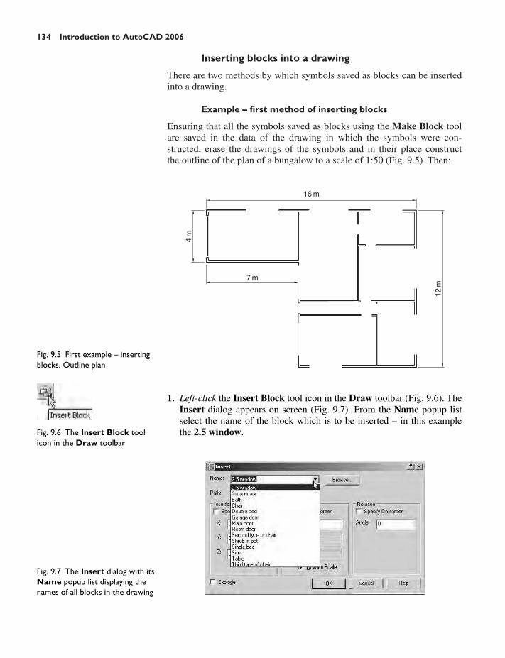
Inserting blocks into a drawing
There are two methods by which symbols saved as blocks can be insertedinto a drawing.
Example – first method of inserting blocks
Ensuring that all the symbols saved as blocks using the Make Block toolare saved in the data of the drawing in which the symbols were con-structed, erase the drawings of the symbols and in their place constructthe outline of the plan of a bungalow to a scale of 1:50 (Fig. 9.5). Then:
134 Introduction to AutoCAD 2006
16 m4
m
7 m
12 m
Fig. 9.5 First example – insertingblocks. Outline plan
1. Left-click the Insert Block tool icon in the Draw toolbar (Fig. 9.6). TheInsert dialog appears on screen (Fig. 9.7). From the Name popup listselect the name of the block which is to be inserted – in this examplethe 2.5 window.Fig. 9.6 The Insert Block tool
icon in the Draw toolbar
Fig. 9.7 The Insert dialog with itsName popup list displaying thenames of all blocks in the drawing
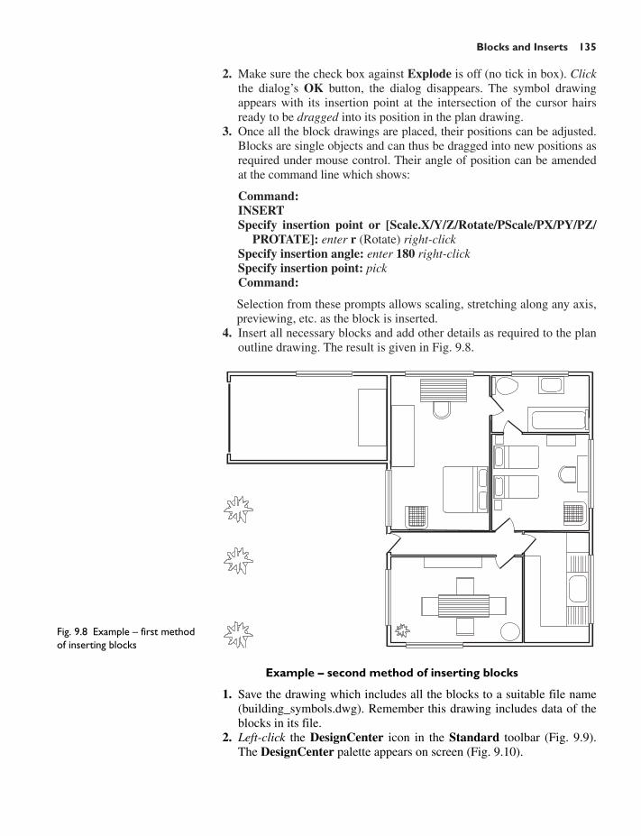
2. Make sure the check box against Explode is off (no tick in box). Clickthe dialog’s OK button, the dialog disappears. The symbol drawingappears with its insertion point at the intersection of the cursor hairsready to be dragged into its position in the plan drawing.
3. Once all the block drawings are placed, their positions can be adjusted.Blocks are single objects and can thus be dragged into new positions asrequired under mouse control. Their angle of position can be amendedat the command line which shows:
Command:INSERTSpecify insertion point or [Scale.X/Y/Z/Rotate/PScale/PX/PY/PZ/
PROTATE]: enter r (Rotate) right-clickSpecify insertion angle: enter 180 right-clickSpecify insertion point: pickCommand:
Selection from these prompts allows scaling, stretching along any axis,previewing, etc. as the block is inserted.
4. Insert all necessary blocks and add other details as required to the planoutline drawing. The result is given in Fig. 9.8.
Blocks and Inserts 135
Fig. 9.8 Example – first methodof inserting blocks
Example – second method of inserting blocks
1. Save the drawing which includes all the blocks to a suitable file name(building_symbols.dwg). Remember this drawing includes data of theblocks in its file.
2. Left-click the DesignCenter icon in the Standard toolbar (Fig. 9.9).The DesignCenter palette appears on screen (Fig. 9.10).

136 Introduction to AutoCAD 2006
Fig. 9.10 The DesignCenterwith the double bed block draggedon screen
3. With the outline plan (Fig. 9.5) on screen the symbols can all bedragged into position from the DesignCenter.
Notes about DesignCenter palette
1. As with other palettes, the DesignCenter palette can be re-sized bydragging the palette to a new size from its edges or corners.
2. Clicks on one of the three icons at the top-right corner of the palette(Fig. 9.11) have the following results:Tree View Toggle – changes from showing two areas – a Folder List
and icons of the blocks within a file – to a single area showing theblock icons.
Preview – a click on the icon opens a small area at the base of the paletteshowing an enlarged view of the selected block icon (Fig. 9.12).
Fig. 9.11 The icons at the top-right corner of theDesignCenter palette
Fig. 9.12 The results of clicks onTree View Toggle, Previewand Description
Fig. 9.9 The DesignCenter iconin the Standard toolbar

Description – a click on the icon opens another small area with adescription of the block.
The Explode and Purge tools
A block is a single object no matter from how many objects it was origi-nally constructed. This enables a block to be dragged about the drawingarea as a single object.
A check box in the bottom left-hand corner of the Insert dialog islabelled Explode (Fig. 9.13). If the check box is ticked, Explode will beset on and when a block is inserted it will be exploded into the objectsfrom which it was constructed.
Another way of exploding a block would be to use the Explode toolfrom the Modify toolbar (Fig. 9.14). A click on the icon or entering x atthe command line brings prompts into the command line:
Command:_explodeSelect objects: pick a block on screen 1 found.Select objects: right-clickCommand:
And the picked object is exploded into its original objects.
The Purge tool
The Purge tool can be called by entering pu at the command line or fromDrawing Utilities in the File drop-down menu (Fig. 9.15). When the toolis called the Purge dialog appears on screen (Fig. 9.16).
Blocks and Inserts 137
Fig. 9.13 The Explode check boxin the Insert dialog
Fig. 9.14 The Explode tool in theModify toolbar
Fig. 9.15 Calling Purge from theFile drop-down menu
The Purge tool can be used to remove the data of blocks within adrawing thus saving file space when a drawing which includes blocks issaved to file.
To use the tool, in its dialog click the Purge button and a sub-dialogappears naming a block to be purged. A click on the Yes button clears thedata of the block from the drawing. Continue until all blocks that are to bepurged are removed.
Take the drawing in Fig. 9.8 (page 135) as an example. If all the blocksare purged from the drawing, the file will be reduced from 145 KB to67 KB when the drawing is saved to disk.
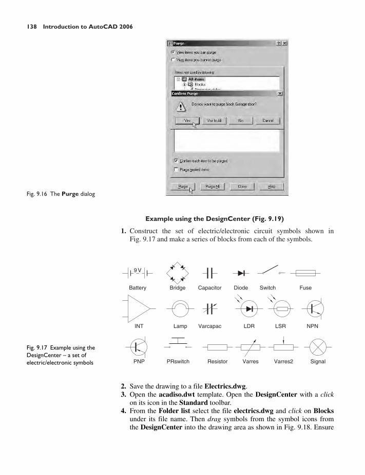
138 Introduction to AutoCAD 2006
Fig. 9.16 The Purge dialog
Example using the DesignCenter (Fig. 9.19)
1. Construct the set of electric/electronic circuit symbols shown inFig. 9.17 and make a series of blocks from each of the symbols.
Battery Bridge Capacitor Diode Switch
INT Lamp Varcapac LDR LSR NPN
PNP PRswitch Resistor Varres Varres2 Signal
Fuse
9 V
Fig. 9.17 Example using theDesignCenter – a set ofelectric/electronic symbols
2. Save the drawing to a file Electrics.dwg.3. Open the acadiso.dwt template. Open the DesignCenter with a click
on its icon in the Standard toolbar.4. From the Folder list select the file electrics.dwg and click on Blocks
under its file name. Then drag symbols from the symbol icons fromthe DesignCenter into the drawing area as shown in Fig. 9.18. Ensure

Blocks and Inserts 139
Fig. 9.18 Example using theDesignCenter
they are placed in appropriate positions in relation to each other toform a circuit. If necessary either Move or/and Rotate the symbolsinto correct positions.
5. Close the DesignCenter palette with a click on the x in the top left-hand corner.
6. Complete the circuit drawing as shown in Fig. 9.19.
6 V
Fig. 9.19 Example using theDesignCenter – the completedcircuit
Note
Fig. 9.19 does not represent an authentic electronics circuit.
Wblocks
Wblocks or written blocks are saved as drawing files in their own rightand are not part of the drawing in which they have been saved.
Example – wblock (Fig. 9.20)
1. Construct a light emitting diode (LED) symbol and enter w at thecommand line. The Write Block dialog appears (Fig. 9.20).

2. Click the button marked with three dots (. . .) to the right of the Filename and path field and from the Browse for Drawing File dialogwhich comes to screen select an appropriate directory. The directoryname appears in the File name and path field. Add LED.dwg at theend of the name.
3. Make sure the Insert units is set to Millimetres in its popup list.4. Click the Select objects button, window the symbol drawing and when
the dialog reappears, click the Pick point button, followed by selectingthe left-hand end of the symbol.
5. Finally click the OK button of the dialog and the symbol is saved in itsselected directory as a drawing file LED.dwg in its own right.
Notes on the DesignCenter
Drawings can be inserted into the AutoCAD window from the DesignCenterby dragging the icon representing the drawing into the window (Fig. 9.21).
140 Introduction to AutoCAD 2006
Fig. 9.20 Example – Wblock
Fig. 9.21 An example of a drawingdragged from the DesignCenter

When such a drawing is dragged into the AutoCAD window, thecommand line shows a sequence such as:
Command:_INSERT Enter block name or [?] �Fig26�: “Chapter07\inserts\Fig26.dwg”
Specify insertion point or [prompts]: pickEnter X scale factor �1�: right-clickEnter Y scale factor �use X scale factor�: right-clickSpecify rotation angle �0�: right-clickCommand:
Revision notes
1. Blocks become part of the drawing file in which they were con-structed.
2. Wblocks become drawing files in their own right.3. Drawings or parts of drawings can be inserted in other drawings with
the Insert Block tool.4. Inserted blocks or drawings are single objects unless either the
Explode check box of the Insert dialog is checked, or the block ordrawing is exploded with the Explode tool.
5. Drawings can be inserted into the AutoCAD drawing area using theDesignCenter.
6. Blocks within drawings can be inserted into drawings from theDesignCenter.
Exercises
1. Construct the building symbols in Fig. 9.22 in a drawing saved assymbols.dwg. Then using the DesignCenter construct a buildingdrawing of the first floor of the house you are living in, making use ofthe symbols. Do not bother too much about dimensions because thisexercise is designed to practise using the idea of making blocks andusing the DesignCenter.
Blocks and Inserts 141
wall
partition
door01
window01
compass
MH pipe
tree02tree01
stair
bath
sink
boiler
cooker
fridge
WC
B
R
C
basin
door02
window02
up_and_over
Fig. 9.22 Exercise 1

2. Construct drawings of the electric/electronics symbols in Fig. 9.17(page 138 ) and save them as blocks in a drawing file electronics.dwg.
3. Construct the electronics circuit given in Fig. 9.23 from the fileelectronics.dwg using the DesignCenter.
142 Introduction to AutoCAD 2006
9 V
Fig. 9.23 Exercise 3
4. Construct the electronics circuit given in Fig. 9.24 from the fileelectronics.dwg using the DesignCenter.
Fig. 9.24 Exercise 4

CHAPTER 10
Other types of file format
Aims of this chapter
1. To introduce Object Linking and Embedding (OLE) and its uses.2. To introduce the use of Encapsulated Postscript (EPS) files.3. To introduce the use of Data Exchange Format (DXF) files.4. To introduce raster files.5. To introduce Xrefs.
Object linking and embedding
First example – copying and pasting (Fig. 10.3)
1. Open any drawing in the AutoCAD 2006 window (Fig. 10.1).2. Left-click Copy Link in the Edit drop-down menu (Fig. 10.1).
143
Fig. 10.1 A drawing in theAutoCAD 2006 window showingCopy Link selected from theEdit drop-down menu
3. Click the AutoCAD 2006 Minimize button and open the Clipboardviewer. The copied drawing appears in the clipboard (Fig. 10.2).

4. Open Microsoft Word and click on Paste in the Edit drop-down menu(Fig. 10.3). The drawing from the Clipboard appears in the MicrosoftWord document (Fig. 10.3).
5. Add text as required.
144 Introduction to AutoCAD 2006
Fig. 10.2 The drawing fromAutoCAD copied to theClipboard
Fig. 10.3 Example – copying andpasting

Notes
1. It is not common practice to have a Clipboard window showing onscreen. The Clipboard usually works in the background and thus it isnot normal practice for it to be seen. It is shown opened here to displayits use in acting as an agent for transposing drawings etc. from oneapplication to another.
2. Similar results can be obtained using the Copy and Copy with BasePoint tools from the Edit drop-down menu of AutoCAD 2006.
3. The drawing could also be pasted back into the AutoCAD window –not that there would be much point in doing so, but anything in theClipboard window can be pasted into other applications.
Second example – EPS file (Fig. 10.5)
1. With the same drawing on screen click on Export . . . in the File drop-down menu. The Export Data dialog appears (Fig. 10.4). Pick Encapsu-lated PS (*.eps) from the Files of type popup list, then enter a suitablefile name (building.eps) in the File name field and click the Save button.
2. Open a desktop publishing application. That shown in Fig. 10.5 isPageMaker.
Other types of file format 145
Fig. 10.4 The Export Datadialog of AutoCAD 2006
3. From the File drop-down menu click Place . . . A dialog appears list-ing files which can be placed in a PageMaker document. Among thefiles named will be building.eps. Double-click that file name and anicon appears, the placing of which determines the position of the *.epsfile drawing in the PageMaker document (Fig. 10.5).
4. Add text as required.5. Save the PageMaker document to a suitable file name.
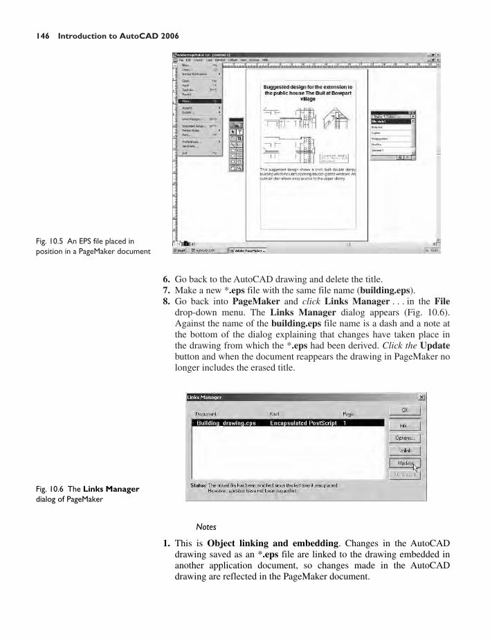
6. Go back to the AutoCAD drawing and delete the title.7. Make a new *.eps file with the same file name (building.eps).8. Go back into PageMaker and click Links Manager . . . in the File
drop-down menu. The Links Manager dialog appears (Fig. 10.6).Against the name of the building.eps file name is a dash and a note atthe bottom of the dialog explaining that changes have taken place inthe drawing from which the *.eps had been derived. Click the Updatebutton and when the document reappears the drawing in PageMaker nolonger includes the erased title.
146 Introduction to AutoCAD 2006
Fig. 10.5 An EPS file placed inposition in a PageMaker document
Fig. 10.6 The Links Managerdialog of PageMaker
Notes
1. This is Object linking and embedding. Changes in the AutoCADdrawing saved as an *.eps file are linked to the drawing embedded inanother application document, so changes made in the AutoCADdrawing are reflected in the PageMaker document.

2. There is actually no need to use the Links Manager because if the filefrom PageMaker is saved with the old *.eps file in place, when it isreopened the file will have changed to the redrawn AutoCAD drawing,without the erased title.
DXF (Data Exchange Format) files
The *.DXF format was originated by Autodesk (publishers of AutoCAD),but is now in general use in most CAD software. A drawing saved to a*.dxf format file can be opened in most other CAD software applications.This file format is of great value when drawings are being exchangedbetween operators using different CAD applications.
Example – DXF file (Fig. 10.8)
1. Open a drawing in AutoCAD. This example is shown in Fig. 10.7.2. Click on Save As . . . in the File drop-down menu and in the Save
Drawing As dialog which appears, click AutoCAD 2006 DXF [*.dxf].
Other types of file format 147
Fig. 10.7 Example – DXF file.Drawing to be saved as a dxf file
3. Enter a suitable file name. In this example this is Fig07. The extension.dxf is automatically included when the Save button of the dialog isclicked (Fig. 10.8).
4. The DXF file can now be opened in the majority of CAD applicationsand then saved to the drawing file format of the CAD in use.
Note
To open a DXF file in AutoCAD 2006, select Open . . . from the Filedrop-down menu and select AutoCAD 2006 DXF [*.dxf] from the popuplist from the Files of type field.

148 Introduction to AutoCAD 2006
Fig. 10.8 The Save Drawing Asdialog set up to save drawings inDXF format
Raster images
A variety of raster files can be placed into AutoCAD 2006 drawings fromthe Select Image File dialog brought to screen with a click on RasterImage . . . in the Insert drop-down menu. In this example the selectedraster file is a bitmap (extension *.bmp) of a rendered 3D model drawingconstructed to the views in an assembly drawing of a lathe tool post (seeChapter 16 for rendering 3D models).
Example – placing a raster file in a drawing (Fig. 10.12)
1. Click Raster Image . . . from the Insert drop-down menu (Fig. 10.9).The Select Image File dialog appears (Fig. 10.10). Click the filename of the image to be inserted – in this example rendering01.bmp.A preview appears in the Preview area of the dialog.
Fig. 10.9 Selecting RasterImage . . . from the Insertdrop-down menu
Fig. 10.10 The Select ImageFile dialog

2. Click the Open button of the dialog. The Image dialog appears(Fig. 10.11).
Other types of file format 149
Fig. 10.11 The Image dialog
3. In the Scale field enter a suitable scale figure. The size of the imagethat will appear in the AutoCAD window can be seen with a click onthe Details button which brings down an extension of the dialog whichshows details about the resolution and size of the image.
4. Click the OK button, the command line shows:
Command:_imageattachSpecify insertion point �0,0�: an outline of the image attached to
the intersection of the cursor cross hairs appears pick a suitablepoint on screen
Command:
And the raster image appears at the picked point (Fig. 10.12).
Note
As can be seen from the Insert drop-down menu (Fig. 10.9), a varietyof different types of raster and other images can be inserted into an Auto-CAD drawing. Some examples are:
Blocks – see Chapter 9.External References (Xrefs) – see later in this chapter.Field name – a click on the name brings up the Field dialog. Practise
inserting various categories of field names from the dialog.Layout – a wizard appears allowing new layouts to be created and saved
for new templates.

150 Introduction to AutoCAD 2006
3D Studio – allows the insertion of images, constructed in the Autodesksoftware 3D Studio, from files with the format *.3ds.
OLE Objects – allows raster images to be placed as OLE images from avariety of other applications.
External References (Xrefs)
If a drawing is inserted into another drawing as an external reference, anychanges made in the original Xref drawing are automatically reflected inthe drawing into which the Xref has been inserted.
Example – Xrefs (Fig. 10.19)
1. Construct the three-view orthographic drawing in Fig. 10.15. Dimen-sions of this drawing will be found on page 239. Save the drawing to asuitable file name.
2. As a separate drawing construct Fig. 10.16. Save it as a wblock withthe name of spindle.dwg and with a base insertion point at one end ofits centre line.
3. In the Insert drop-down menu click Xref Manager . . . The XrefManager dialog appears (Fig. 10.13).
4. Click its Attach button. The Select Reference File dialog appears.Select the spindle drawing from the file list. Its name appears in Name
Fig. 10.13 The Xref Managerdialog
Fig. 10.12 Example – placing araster file in a drawing

Other types of file format 151
Fig. 10.14 The ExternalReference dialog
field of another dialog External Reference (Fig. 10.14). Click its OKbutton.
5. The spindle drawing appears on screen ready to be dragged intoposition. Place it in position as indicated in Fig. 10.17.
6. Save the drawing with its Xref to its original file name.
Fig. 10.15 Example – Xrefs –original drawing
Fig. 10.16 The spindle.dwgdrawing

7. Open the drawing spindle.dwg and make changes as shown in Fig. 10.18.8. Now reopen the original drawing. The Xref within the drawing
has changed in accordance with the alterations to the spindle drawing(Fig. 10.19).
Note
In this example to ensure accuracy of drawing the Xref will need to beexploded and parts of the spindle changed to hidden detail lines.
Multiple Document Environment (MDE)
1. Open several drawings in AutoCAD – in this example four separatedrawings have been opened.
2. In the Window drop-down menu, click Tile Horizontally. The fourdrawings rearrange as shown in Fig. 10.20.
Note
The names of the drawings appear at the base of the Window drop-downmenu, showing their directories, file names and file name extensions.
Revision notes
1. When an *.eps file is inserted from AutoCAD 2006 into a document,subsequent changes in the original drawing are reflected in the inserted*.eps file in the document.
2. The Edit tools Copy with Base Point, Copy and Copy Link enableobjects from AutoCAD 2006 to be copied for Pasting onto otherapplications.
3. Objects can be copied from other applications to be pasted into theAutoCAD 2006 window.
4. Drawings saved in AutoCAD as DXF (*.dxf) files can be opened inother CAD applications.
5. Similarly drawings saved in other CAD applications as *.dxf files canbe opened in AutoCAD 2006.
6. Raster files of the format types *.bmp, *.jpg, *.pcx, *.tga, *.tif,among other raster type file objects, can be inserted into AutoCAD2006 drawings.
7. Drawings saved to the Encapsulated Postscript (*.eps) file format canbe inserted into documents of other applications.
8. Changes made in a drawing saved as an *.eps file will be reflected inthe drawing inserted as an *.eps file in another application.
9. A number of drawings can be opened in the AutoCAD 2006window.
152 Introduction to AutoCAD 2006
Fig. 10.18 The revisedspindle.dwg drawing
Fig. 10.19 Example – Xrefs
Fig. 10.17 The spindle in place inthe original drawing

Other types of file format 153
Fig. 10.20 Four drawings in theMultiple DocumentEnvironment
The hatched parts of the Xref drawing were then changed using adifferent hatch pattern. The result of the change in the Xref is shown inFig. 10.22.
Exercises
1. Fig. 10.21 shows a pattern formed by inserting an Xref and then eithercopying or arraying the Xref.
Fig. 10.21 Exercise 1 – originalpattern

154 Introduction to AutoCAD 2006
Fig. 10.22 Exercise 1
Fig. 10.23 Exercise 2 – arendering of the holders androller
Hole ∅80
∅80 ∅
100
40 250
R50
R120
R50
R15
170
402090
Fig. 10.24 Exercise 2 – details ofthe parts of the roller and holders
Construct a similar Xref drawing, insert an Xref, array or copy toform the pattern, then change the hatching, save the Xref drawing andnote the results.
2. Fig. 10.23 is a rendering of a roller between two end holders. Fig. 10.24gives details of the end holders and the roller in orthographic projections.
Construct a full size front view of the roller and save to a file nameroller.dwg. Then as a separate drawing construct a front view of thetwo end holders in their correct positions to receive the roller and saveto the file name assembly.dwg.
Insert the roller drawing into the assembly drawing as an Xref.

Other types of file format 155
20 20
20
R15
R15
Fig. 10.25 The amended Xrefdarwing
4. Using Copy from the Insert drop-down menu, copy a drawing fromAutoCAD 2006 into a Microsoft Word document. An example is givenin Fig. 10.27. Add some appropriate text.
3. Click Raster Image . . . in the Insert drop-down menu and insert aJPEG image (*.jpg file) of a photograph into the AutoCAD 2006window. An example is given in Fig. 10.26.
Open the roller.dwg and change its outline as shown in Fig. 10.25.Save the drawing. Open the assembly.dwg and note the change in theinserted Xref.
Fig. 10.26 Exercise 3 – example

156 Introduction to AutoCAD 2006
Fig. 10.27 Exercise 4 – anexample
5. The plan in Figs 10.1, 10.2 and 10.3 is incorrect in that some detailshave been missed from the drawing. Can you identify the error?

CHAPTER 11
Sheet sets
Aims of this chapter
1. To introduce sheet sets.2. To give an example of a sheet set based on the design of a two-storey
house.
Sheet sets
When anything is to be manufactured or constructed, whether it be abuilding, an engineering design, an electronics device or any other formof manufactured artefact, a variety of documents, many in the form oftechnical drawings, will be needed to convey to those responsible forconstructing the design information necessary to be able to proceedaccording to the wishes of the designer. Such sets of drawings may bepassed between the people or companies responsible for the construc-tion, enabling all those involved to make adjustments or suggestchanges to the design. In some cases there may well be a considerablenumber of drawings required in such sets of drawings. In AutoCAD2006 all the drawings from which a design is to be manufactured can begathered together in a sheet set. This chapter shows how a muchreduced sheet set of drawings for the construction of a house at 62Pheasant Drive can be formed. Some other drawings, particularly detaildrawings, would be required in this example, but to save page space, thesheet set described here consists of only four drawings and a subset ofanother four.
Example – a sheet set for 62 Pheasant Drive
1. Construct a template 62 Pheasant Drive.dwt based upon theacadiso.dwt template, but including a border and a title block. Save thetemplate in a Layout1 format. An example of the title block from oneof the drawings constructed in this template is shown in Fig. 11.1.
2. Construct each of the drawings which will form the sheet set in thisdrawing template. The whole set of drawings is shown in Fig. 11.10 onpage 161. Save the drawings in a directory – in this example this hasbeen given the name 62 Pheasant Drive.
157

3. Click New Sheet Set in the File drop-down menu (Fig. 11.2). The firstof a series of Create Sheet Set dialogs appears – the Begin dialog(Fig. 11.3). Click the radio button next to Existing drawings, followedby a click on the Next button and the next dialog Sheet Set Detailsappears (Fig. 11.4).
158 Introduction to AutoCAD 2006
62 Pheasant Drive
Title:
2Drawing No:Scale:
1:50Date:
12:09:07
Building planFig. 11.1 The title block fromDrawing number 2 of thesheet set
Fig. 11.2 Selecting New SheetSet . . . from the File drop-downmenu
Fig. 11.3 The first of the CreateSheet Set dialogs – Begin

4. Enter details as shown in the dialog in Fig. 11.4. Then click the SheetSet Properties button. The Sheet Set Properties dialog appears show-ing the properties of the proposed sheet set (Fig. 11.5). If satisfied withthe details in the dialog, click its OK button. The Sheet Set Detailsdialog reappears. Click its Next button to call the next dialog, theChoose Layouts dialog, to screen (Fig. 11.6).
Sheet sets 159
Fig. 11.4 The Sheet Set Detailsdialog
Fig. 11.5 The Sheet SetProperties dialog
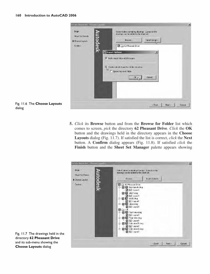
5. Click its Browse button and from the Browse for Folder list whichcomes to screen, pick the directory 62 Pheasant Drive. Click the OKbutton and the drawings held in the directory appears in the ChooseLayouts dialog (Fig. 11.7). If satisfied the list is correct, click the Nextbutton. A Confirm dialog appears (Fig. 11.8). If satisfied click theFinish button and the Sheet Set Manager palette appears showing
160 Introduction to AutoCAD 2006
Fig. 11.6 The Choose Layoutsdialog
Fig. 11.7 The drawings held in thedirectory 62 Pheasant Driveand its sub-menu showing theChoose Layouts dialog

the drawings which will be in the 62 Pheasant Drive sheet set(Fig. 11.9). Fig. 11.10 shows the complete set and sub set of the eightdrawings in the 62 Pheasant Drive sheet set.
Sheet sets 161
Shooters Way
Scale:
Scale:
Scale:
Title:
Scale:
Title:
10,000
4,00
0
3,90
0
7,000
2,500
Existing boundary Pheasant Drive
Boardedfences
Upper floor
Bedroom 1
Bedroom3
Bedroom2
LoungeDiningroom
Kitchen
Front
Rear
Side
Side
Ground floor
62 Pheasant Drive
Title:
Scale: Date: Drawing No:
1:100 12:09:07 4
Elevations
62 Pheasant Drive
Side view from West
Scale:1:50 13:09:07 4D
Date: Drawing No:
Title:
Sheet Set
Sub set
Fig. 11.8 The Confirm dialog
Fig. 11.9 The Sheet SetManager for 62 PheasantDrive
Fig. 11.10 The eight drawingsin the 62 Pheasant Drive sheetset

Notes
1. If any of the eight drawings in the sheet set are subsequently amendedor changed, when the drawings are opened again from the 62 Pheas-ant Drive Sheet Set Manager the drawing will include any changes oramendments.
2. Drawings can only be placed into sheet sets if they have been saved ina Layout screen. Note that all the drawings shown in the 62 PheasantDrive Sheet Set Manager have Layout1 after the drawing namesbecause each has been saved after being placed in a Layout1 screen.
3. Sheet sets in the form of DWF (Design Web Format) files can be sentvia email to others who are using the drawings or placed on anintranet. The method of producing a DWF for the 62 Pheasant DriveSheet Set follows.
62 Pheasant Drive DWF
1. In the 62 Pheasant Drive Sheet Set Manager click the Publishto DWF icon (Fig. 11.11). The Select DWF File dialog appears(Fig. 11.12). Enter 62 Pheasant Drive in the File name field followedby a click on the Select button. An icon in the bottom right-hand cor-ner of the AutoCAD 2006 window starts fluctuating in shape showingthat the DWF file is being processed (Fig. 11.13). When the iconbecomes stationary again a warning balloon appears stating that thePublish Job is completed (Fig. 11.14).
162 Introduction to AutoCAD 2006
2. Right-click on the icon at the bottom right-hand corner of the Auto-CAD 2006 window. The right-click menu (Fig. 11.15) appears.
3. Click View DWF File . . . from the right-click menu. The AutodeskDWF Viewer window appears showing the 62 Pheasant Drive.dwf
Fig. 11.11 The Publish to DWFicon in the Sheet Set Manager
Fig. 11.12 The Select DWF Filedialog

file (Fig. 11.16). Click on any of the icons of the thumbnails of thedrawings in the viewer and the drawing appears in the right-hand areaof the viewer.
4. If required the DWF Viewer file can be sent between people by emailas an attachment, opened in a company’s intranet or, indeed, includedwithin an Internet web page.
Sheet sets 163
Revision notes
1. To start off a new sheet set, click New Sheet Set . . . in the File drop-down menu.
2. Sheet sets can only contain drawings saved in Layout form.3. Sheet sets can be published as Design Web Format (*.dwf) files
which can be sent between offices by email, published on an intranetor published on a web page.
4. Sub sets can be included in sheet sets.5. Changes or amendments made to any drawings in a sheet set are
reflected in the sheet set drawings when the sheet set is opened.
Fig. 11.13 The Publish Job inProgress icon
Fig. 11.14 The Publish Jobwarning balloon
Fig. 11.15 The right-click menufrom which View DWF File . . .is selected
Fig. 11.16 The Autodesk DWFViewer showing details of the 62Pheasant Drive.dwf file

Exercises
1. Fig. 11.17 is an exploded orthographic projection of the parts of a pis-ton and its connecting rod. There are four parts in the assembly. Smalldrawings of the required sheet set are shown in Fig. 11.18.
Construct the drawing in Fig. 11.17 and also the four drawings ofits parts. Save each of the drawings in a Layout1 format and constructthe sheet set which contains the five drawings.
164 Introduction to AutoCAD 2006
Holes ∅10
Dimensions in millimetres
Hole ∅20
Sphere ∅64 Sphere ∅40
Pin 70 x ∅20
∅70
20 20150 70
DO NOT SCALE
63
58
R20
45
A. READER Scale 1:1 Date: 23:6:2005 Part: 8/45+8/46 PISTON & CONNECTING ROD
45
20
8
25
M10
30
Holes ∅10
Dimensions in millimetres
Hole ∅20
Hole ∅20
Hole ∅20
Hole ∅20
Sphere ∅64
Sphere ∅64 Sphere ∅40
Sphere ∅40
Dimensions in millimetres
Dimensions in millimetres
Sphere ∅54
Pin 70 x ∅20
∅70
∅70
20 20150
150
70DO NOT SCALE
DO NOT SCALE
DO NOT SCALE
DO NOT SCALE
Dimensions in millimetres DO NOT SCALE
20
63
R10
58
45
Cham 2x2
Pin 70x∅2030
35
M10
6358
R20
R10
R8
R10
35
45
A. READER Scale 1:1 Date: 23:6:2005
A. Reader Scale 1:1 Date: 23:6:2005
Part: 8/45+8/46
Part: 8/45
A. Reader Scale 1:1 Date: 23:6:2005 Part: 8/48
A. Reader Scale 1:1 Date: 23:6:2005 Part: 8/46
A. Reader Scale 1:1 Date: 23:6:2005 Parts: 8/46 & 47 BOLT & PIN
PISTON & CONNECTING ROD
23
20
20
2522
8
8
25
M10
30
Construct the DWF file of the sheet set. Experiment sending it to afriend via email as an attachment to a document, asking them to returnthe whole email to you without changes. When the email is returned,open its DWF file and click each drawing icon in turn to check the con-tents of the drawings.
Fig. 11.17 Exercise 1 – theexploded orthographic projection
Fig. 11.18 Exercise 1 – the fivedrawings in the sheet set

Note
Fig. 11.19 shows a DWF for the sheet set from exercise 1 with the addi-tion of a sixth drawing which is a 3D exploded model drawing of the fiveparts of the piston and connecting rod which has been Gouraud shaded –see Chapter 16. This illustration has been included here to show that suchshaded 3D models can be included in a sheet set.
Sheet sets 165
2. Construct a similar sheet set as in the answer to exercise 1 from theexploded orthographic drawing of a Machine adjusting spindle givenin Fig. 11.20.
130
1 2
4
A A
3 5 68
10
45 15 1512
24
100
25
124080
28
40°
18
7
M6
6
5
R6
Part No.
123456
Name of part
SPINDLE AND PINSHOULDER WASHERSBRACKETLOCKSCREWWASHERHANDLE
MACHINE ADJUSTING SPINDLE
∅24
∅12∅24
Tapped M10
Hole ∅10
∅90
26x∅3R12
∅30
Fig. 11.19 The DWF of the sheetset which includes the shaded3D model
Fig. 11.20 Exercise 2

166
CHAPTER 12
Building drawing
Aim of this chapter
To show that AutoCAD 2006 is a suitable CAD software package for theconstruction of building drawing.
Building drawings
There are a number of different types of drawings related to the construc-tion of any form of building. As fairly typical examples of a set of buildingdrawings, in this chapter, seven drawings are shown related to the con-struction of an extension to an existing two-storey house (44 RidgewayRoad). These show:
1. A site plan of the original two-storey house, drawn to a scale of 1:200(Fig. 12.1).
Car park
MeetingHall
Fences
Ridgeway Road
Sum
mer
s R
oad
44 Ridgeway Road
Site planTitle:
1:200Scale:
10:03:08Date: Drawing No:
1
Fig. 12.1 A site plan

Building drawing 167
2. A site layout plan of the original house, drawn to a scale of 1:100(Fig. 12.2).
13.00 m
5.75 m
6.00
m8.
50 m
Ridgeway RoadMH
MH
1:100 11:03:08
Site layout
2
Sum
mer
s R
oad
Scale:
Title:
Date: Drawing No:
44 Ridgeway Road
Fig. 12.2 A site layout plan
3. Floor layouts of the original house, drawn to a scale of 1:50 (Fig. 12.3).
WC
UTILITYROOM KITCHEN
SITTINGROOM
HALL
GROUND FLOOR5.75 m 44 Ridgeway Road
1:50 14:03:08 3
Floor layoutsTitle:
Scale: Date: Drawing No:
FIRST FLOOR
BEDROOM 1
BEDROOM 2BED 3
SPAREROOM
8.50
m
Fig. 12.3 Floor layouts of theoriginal house

168 Introduction to AutoCAD 2006
4. Views of all four sides of the original house, drawn to a scale of 1:50(Fig. 12.4).
South East
North West
44 Ridgeway RoadScale: Date: Drawing No:
Title: Views
1:50 13:03:08 4Fig. 12.4 Views of the originalhouse
5. Floor layouts including the proposed extension, drawn to a scale of1:50 (Fig. 12.5).
NEW LAYOUTGROUND FLOOR
KITCHEN
UTILITYROOM
SITTINGROOM
DININGROOM
HALL
WC
3.25 m
SPAREROOM
BEDROOM 1
BEDROOM 2
BEDROOM 4
BEDROOM 3BATH
NEW LAYOUTFIRST FLOOR
44 Ridgeway RoadScale:
Title:
Date: Drawing No:1:50 17:03:08 5
Revised floor layoutsFig. 12.5 Floor layouts of theproposed extension

Building drawing 169
South East
North West
44 Ridgeway RoadScale: Date: Drawing No:
Title: Revised views1:50 18:03:08 6Fig. 12.6 Views including the
proposed extension
7. A sectional view through the proposed extension, drawn to a scale of1:50 (Fig. 12.7).
44 Ridgeway Road
Section through revision
Scale:
Title:
Date: Drawing No:1:50 20:30:08 7
Fig. 12.7 A section through theproposed extension
6. Views of all four sides of the house including the proposed extension,drawn to a scale of 1:50 (Fig. 12.6).
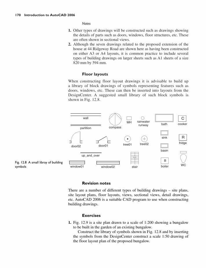
170 Introduction to AutoCAD 2006
Notes
1. Other types of drawings will be constructed such as drawings showingthe details of parts such as doors, windows, floor structures, etc. Theseare often shown in sectional views.
2. Although the seven drawings related to the proposed extension of thehouse at 44 Ridgeway Road are shown here as having been constructedon either A3 or A4 layouts, it is common practice to include severaltypes of building drawings on larger sheets such as A1 sheets of a size820 mm by 594 mm.
Floor layouts
When constructing floor layout drawings it is advisable to build upa library of block drawings of symbols representing features such asdoors, windows, etc. These can then be inserted into layouts from theDesignCenter. A suggested small library of such block symbols isshown in Fig. 12.8.
wall
partition
door01door02
up_and_over
window01 window02 stair boiler WC
basin
fridge
B
sink
cookerbathrainwaterrunway
MH
compass
tree01 tree02
C
R
Fig. 12.8 A small libray of buildingsymbols
Revision notes
There are a number of different types of building drawings – site plans,site layout plans, floor layouts, views, sectional views, detail drawings,etc. AutoCAD 2006 is a suitable CAD program to use when constructingbuilding drawings.
Exercises
1. Fig. 12.9 is a site plan drawn to a scale of 1:200 showing a bungalowto be built in the garden of an existing bungalow.
Construct the library of symbols shown in Fig. 12.8 and by insertingthe symbols from the DesignCenter construct a scale 1:50 drawing ofthe floor layout plan of the proposed bungalow.

Building drawing 171
Pavement
Existingbungalow
Fence
21 m
12.5 m1 m
7 m 15
m
Gar
age
7 m
× 2
.5 m
Lounge7 m × 4 m
Kitchen5 m × 2.5 m
Bed 13.5 m ×
3.5 m
Bed 23.5 m ×3.5 m
WC
Bat
hroo
m3.
5 m
× 2
m
83°
Bou
ndar
y fe
nce
19 m
long
OUT-HOUSE
6.500 m
HOUSE
Boundary fence 34 m long
4.5
m 12.000 m3
m11
.000
m
Step
3.00
0 m
1.500 m
7.000 mStep
5 m
100°
Boundary fence 28 m long
Par
chm
ent R
oad
Fig. 12.9 Exercise 1
Fig. 12.10 Exercise 2
2. Fig. 12.10 is a site plan of a two-storey house to be built on a buildingplot.
Design and construct to a scale 1:50, a suggested pair of floor layoutsfor the two floors of the proposed house.
3. Fig. 12.11 shows a scale 1:100 site plan for the proposed bungalow at4 Caretaker Road. Construct the floor layout for the proposed house asshown in the drawing in Fig. 12.12.

172 Introduction to AutoCAD 2006
MH
MH
9.000
9.000
8.00
05.
700
PLOT 4 Soakaway
Dimensions in metres
A. STUDENT SCALE 1:100 SITE PLAN – PLOT 4 CARETAKER ROAD
Caretaker RoadMH
Fig. 12.11 Exercise 3 – site plan
4.000 4.000
4.00
04.
000
KITCHEN
LIVINGROOM
BEDROOM1
BEDROOM2
9.000
A. STUDENT BUILDING PLAN PLOT 4 CARETAKER ROAD
SCALE 1:50
BATH& WC
Fig. 12.12 Exercise 3

CHAPTER 13
Introducing 3D modelling
Aims of this chapter
1. To introduce all the tools used for the construction of 3D solidmodels.
2. To give examples of the construction of 3D solid models using all thetools from the Solids toolbar.
3. To give examples of 2D outlines suitable as a basis for the constructionof 3D solid models.
4. To give examples of constructions involving the Boolean operators –Union, Subtract and Intersect.
Introduction
As shown in Chapter 1 the AutoCAD coordinate system includes a thirdcoordinate direction Z, which has not been used so far when dealingwith 2D drawings in previous chapters. 3D model drawings make use ofthis third Z coordinate. 3D solid model drawings are mainly constructedusing tools from the four toolbars Solids, Solids Editing, Surfaces andRender.
The toolbars containing Solid and Render tools
The tools in the four toolbars containing the majority of the tools forconstructing and rendering 3D solids and surfaces described in thisbook are shown in Fig. 13.1. When calling the tools from these fourtoolbars, the four same methods apply as are used when constructing2D drawings:
1. A click on a tool icon in a toolbar brings the selected tool intoaction.
2. A click on the name of a tool from a drop-down menu brings thetool into action.
3. Entering the tool name at the command line in the command window,followed by pressing the Return button of the mouse or the Returnkey of the keyboard, brings the tool into action.
4. Some of the 3D tools have an abbreviation which can be entered at thecommand line instead of its full name.
173

174 Introduction to AutoCAD 2006
Notes
1. When constructing 2D drawings no matter which method is used,most operators will use a variety of these four methods. Calling a toolresults in prompts sequences appearing at the command prompt as inthe following example:
Command: enter box right-clickSpecify corner of box or [CEnter]: enter 90,120 right-clickSpecify corner or [Cube/Length]:
Or, if the tool is called from an icon or from a drop-down menu:
Command:_boxSpecify corner of box or [CEnter]: enter 90,120 right-clickSpecify corner or [Cube/Length]:
2. In the chapters which follow, once the prompts sequences for a tool aregiven as in the example above, if the tool’s sequences are to be repeated,they may be replaced by an abbreviated form such as:
Command: box[prompts]: 90,120[prompts]:
Examples of 3D drawings using the 3D Face tool
The following two examples demonstrate the construction of 3D facesusing the 3D Face tool from the Surfaces toolbar. A 3D face is a triangularor quadrilateral flat (planar) or non-planar surface – i.e. a surface witheither three or four edges in 3D space. Lines or other surfaces behind 3Dfaces can be hidden by using the Hide tool.
Fig. 13.1 The four toolbars withtheir tool icons

Introducing 3D modelling 175
First example – 3D Face tool (Fig. 13.2)
1. At the command line:
Command: enter 3dface right-clickSpecify first point or [Invisible]: enter 60,230 right-clickSpecify second point or [Invisible]: enter 60,110 right-clickSpecify third point or [Invisible] �exit�: enter 190,110,150 right-clickSpecify fourth point or [Invisible] �create three-sided face�: enter
190,230,150 right-clickSpecify third point or [Invisible] �exit�: right-clickCommand:
2. Call the Mirror tool and mirror the 3D face about 190,110 and 190,230.3. Click on View in the menu bar and on 3D Views in the drop-down
menu which appears, and click again on SW Isometric in the sub-menuwhich comes on screen alongside the drop-down menu.
4. Click on the Hide tool from the View drop-down menu.After HIDE, part of the right-hand 3D face has been hidden behind theleft-hand face.
Fig. 13.2 First example – 3DFace tool
Before HIDE After HIDE60,230
60,110
190,110,150
190,230,150
Second example – 3D Face tool (Fig. 13.3)
It is assumed in this example that the reader understands how to enter 3Dcoordinates and how to place the screen in various 3D Views from theView drop-down menu.
1. Click on View in the menu bar and again on 3D Views in the drop-down menu. Click again on Front in the sub-menu which appears.
2. Call Zoom and zoom to 1.3. Call the 3D Face tool:
Command: 3dface[prompts]: 130,0[prompts]: 250,0[prompts]: i (for Invisible)[prompts]: 250,110[prompts]: 130,110[prompts]: 190,250
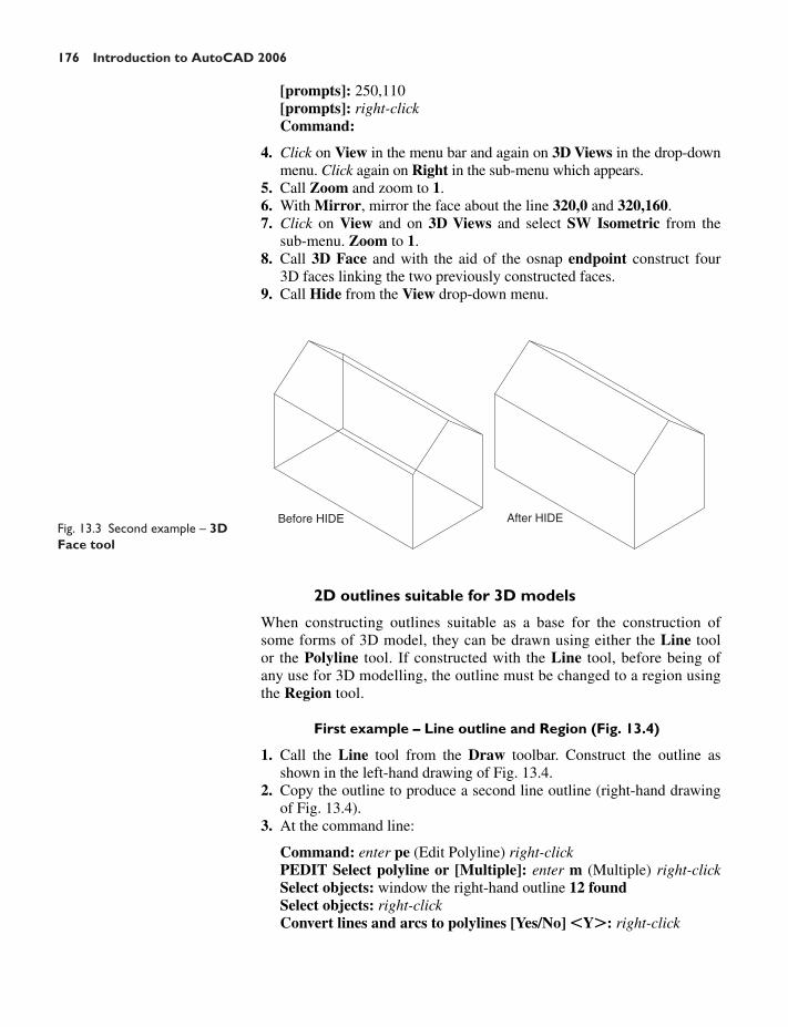
176 Introduction to AutoCAD 2006
Fig. 13.3 Second example – 3DFace tool
Before HIDE After HIDE
2D outlines suitable for 3D models
When constructing outlines suitable as a base for the construction ofsome forms of 3D model, they can be drawn using either the Line toolor the Polyline tool. If constructed with the Line tool, before being ofany use for 3D modelling, the outline must be changed to a region usingthe Region tool.
First example – Line outline and Region (Fig. 13.4)
1. Call the Line tool from the Draw toolbar. Construct the outline asshown in the left-hand drawing of Fig. 13.4.
2. Copy the outline to produce a second line outline (right-hand drawingof Fig. 13.4).
3. At the command line:
Command: enter pe (Edit Polyline) right-clickPEDIT Select polyline or [Multiple]: enter m (Multiple) right-clickSelect objects: window the right-hand outline 12 foundSelect objects: right-clickConvert lines and arcs to polylines [Yes/No] �Y�: right-click
[prompts]: 250,110[prompts]: right-clickCommand:
4. Click on View in the menu bar and again on 3D Views in the drop-downmenu. Click again on Right in the sub-menu which appears.
5. Call Zoom and zoom to 1.6. With Mirror, mirror the face about the line 320,0 and 320,160.7. Click on View and on 3D Views and select SW Isometric from the
sub-menu. Zoom to 1.8. Call 3D Face and with the aid of the osnap endpoint construct four
3D faces linking the two previously constructed faces.9. Call Hide from the View drop-down menu.

Introducing 3D modelling 177
4. Left-click on the Region tool in the Draw toolbar (Fig. 13.5). Thecommand line shows:
Command:_regionSelect objects: window the left-hand drawing 12 foundSelect objects: right-click1 loop extracted1 Region createdCommand:
And the Line outline is changed to a region. Either of the outlines cannow be used when constructing some types of 3D model.
Second example – Union, Subtract and regions (Fig. 13.6)
1. Construct drawing 1 of Fig. 13.6 and with the Copy tool, copy thedrawing three times to produce drawings 2, 3 and 4.
2. With the Region tool change all the outlines into regions.
Fig. 13.4 First example – Lineoutline and Region
Outline constructedusing Line tool
2060
20
20 100 20
Line outline changedto a region
Fig. 13.5 The Region tool icon inthe Draw toolbar
Fig. 13.6 Second example –Union, Subtract and regions
After UnionSubtractregionfrom
Union
Union of2 regions70
60 10
60
30
R25
1
2
3
4
Enter an option [prompts]: enter j (Join) right-click12 segments added to polyline.Command:
And the Line outline is changed to a polyline.

178 Introduction to AutoCAD 2006
3. Drawing 2 – call the Union tool from the Solids Editing toolbar(Fig. 13.7). The command line shows:
Command:_unionSelect objects: pick the left-hand region 1 foundSelect objects: pick the circular region 1 found, 2 totalSelect objects: pick the right-hand region 1 found, 3 totalCommand:
4. Drawing 3 – with the Union tool form a union of the left-hand regionand the circular region.
5. Drawing 4 – call the Subtract tool from the Solids Editing toolbar(Fig. 13.8). The command line shows:
Command:_subtract Select solids and regions to subtract from . . .Select objects: pick the region just formed 1 foundSelect objects: right-clickSelect solids and regions to subtract: pick the right-hand region 1 foundSelect objects: right-clickCommand:
Third example – Intersection and regions (Fig. 13.9)
1. Construct drawing 1 of Fig. 13.9.2. With the Region tool, change the three outlines into regions.
Fig. 13.8 The Subtract tool iconfrom the Solids Editing toolbar
Fig. 13.7 The Union tool iconfrom the Solids Editing toolbar
50
R55 R55
Circle centres 50 apart Intersect onthe 2 circles
Intersectwith rectangle
90
21 3
Fig. 13.9 Third example –Intersection and regions
Fig. 13.10 The Intersect toolicon from the Solids Editingtoolbar
3. With the Copy tool, copy the three regions.4. Drawing 2 – call the Intersect tool from the Solids Editing toolbar
(Fig. 13.10). The command line shows:
Command:_intersectSelect objects: pick one of the circles 1 foundSelect objects: pick the other circle 1 found, 2 totalSelect objects: right-clickCommand:
And the two circular regions intersect with each other to form a region.5. Drawing 3 – repeat using the Intersect tool on the intersection of the
two circles and the rectangular region.

Introducing 3D modelling 179
The Extrude tool
The Extrude tool can be called either, with a click on its tool icon in theSolids toolbar (Fig. 13.11), or by entering extrude or its abbreviation extat the command line.
Fig. 13.11 The Extrude tool iconfrom the Solids toolbar
Extrude can also be called from the Draw drop-down menu – click onDraw in the menu bar and when the Draw drop-down menu appears,click on Solids in the drop-down menu and again on Extrude in the sub-menu which then appears (Fig. 13.12).
Examples of the use of the Extrude tool
The three examples of forming regions given in Figs 13.4, 13.6 and 13.9are used here to show the results of using the Extrude tool.
First example – Extrude (Fig. 13.14)
From the first example of forming a region:
1. Call the Extrude tool. The command line shows:
Command:_extrudeCurrent wire frame density: ISOLINES�4Select objects: pick the region 1 foundSelect objects: right-clickSpecify height of extrusion or [Path]: enter 50 right-clickSpecify angle of taper for extrusion �0�: right-clickCommand:
2. Click View in the menu bar, followed by a click on 3D Views in thedrop-down menu which appears, followed by another click on SWIsometric in the 3D Views sub-menu (Fig. 13.13). The extrusionappears in an isometric view.
3. Call Zoom and zoom to 1.4. At the command line:
Command: enter hi (abbreviation for Hide) right-clickHIDE Regenerating modelCommand:
Fig. 13.12 Calling Extrude fromthe Draw drop-down menu

180 Introduction to AutoCAD 2006
Notes
1. In the above example we made use of one of the isometric viewspossible using the 3D Views sub-menu of the View drop-downmenu. These views from this sub-menu will be used frequently inexamples to show 3D solid model drawings in a variety of positionsin 3D space.
2. Note also the use of the Hide tool. Extruded polylines or regions aremade up from 3D faces (3D meshes). When Hide is called, linesbehind the 3D meshes become invisible on screen.
3. Hide can also be called from the View drop-down menu, but thequickest method of calling the tool is to enter hi at the command line,followed by a right-click.
4. Note the Current wire frame density: ISOLINES�4 in the promptssequence when Extrude is called. The setting of 4 is suitable when
Fig. 13.13 The 3D Viewssub-menu from the Viewdrop-down menu
Before Hide After HideFig. 13.14 First example –Extrude

Introducing 3D modelling 181
extruding plines or regions consisting of straight lines, but when arcsare being extruded it may be better to set ISOLINES to a higher figureas follows:
Command: enter isolines right-clickEnter new value for ISOLINES �4�: enter 16 right-clickCommand:
Second example – Extrude (Fig. 13.15)
From the second example of forming a region:
1. Set ISOLINES to 16.2. Call the Extrude tool. The command line shows:
Command:_extrudeCurrent wire frame density: ISOLINES�16Select objects: pick the region 1 foundSelect objects: right-clickSpecify height of extrusion or [Path]: enter 50 right-clickSpecify angle of taper for extrusion �0�: enter 5 right-clickCommand:
3. Click SW Isometric in the 3D Views sub-menu of the View drop-down menu (see Fig. 13.13).
4. Zoom to 1.5. Call Hide.
Fig. 13.15 Second example –Extrude
Third example – Extrude (Fig. 13.16)
From the third example of forming a region:
1. Place the screen in the 3D Views/Front view (see Fig. 13.13).2. Construct a semicircular arc from the centre of the region.3. Place the screen in the 3D Views/Top view.4. With the Move tool, move the arc to the centre of the region.5. Place the screen in the 3D Views/SW Isometric view.

182 Introduction to AutoCAD 2006
6. Set ISOLINES to 24.7. Call the Extrude tool. The command line shows:
Command:_extrudeCurrent wire frame density: ISOLINES�24Select objects: pick the region 1 foundSelect objects: right-clickSpecify height of extrusion or [Path]: enter p right-clickSelect extrusion path or [Taper angle]: pick the pathCommand:
The Revolve tool
The Revolve tool can be called either with a click on its tool icon in theSolids toolbar (Fig. 13.17), or by a click on its name in the Solids sub-menuof the Draw drop-down menu, or by entering revolve, or its abbreviationrev, at the command line.
Path
Object
The extrusion
Fig. 13.16 Third example –Extrude
Start point for axis Axis endpoint280
1545
10 85 R10
45
R510
Fig. 13.17 The Revolve tool iconfrom the Solids toolbar
Fig. 13.18 First example –Revolve. The closed pline
Examples of the use of the Revolve tool
Solids of revolution can be constructed from closed plines or from regions.
First example – Revolve (13.19)
1. Construct the closed polyline in Fig. 13.18.
2. Set ISOLINES to 24.3. Call the Revolve tool. The command line shows:
Command:_revolveCurrent wire frame density�24Select objects: pick the polylineSelect objects: right-clickSpecify start point for axis of revolution or define axis by
[Object/X (axis)/Y (axis)]: pick

Introducing 3D modelling 183
Second example – Revolve (Fig. 13.21)
1. Place the screen in the 3D Views/Front view. Zoom to 1.2. Construct the pline outline (Fig. 13.20).3 Set ISOLINES to 24.4. Call the Revolve tool and construct a solid of revolution.5. Place the screen in the 3D Views/SW Isometric view.6. Call Hide.
Fig. 13.19 First example –Revolve
4
4
40
Semi-ellipse basedon 180 × 100 axes
Fig. 13.20 Second example –Revolve. The pline outline
Fig. 13.21 Second example –Revolve
Third example – Revolve (Fig. 13.23)
1. Construct the pline in Fig. 13.22. The drawing must be either a closedpline or a region.
2. Call Revolve and form a solid of revolution through 180�.
Specify endpoint of axis: pickSpecify angle of revolution �360�: right-clickCommand:
4. Place in the 3D Views/SW Isometric view.5. Call Hide.

184 Introduction to AutoCAD 2006
3D objects
At the command line:
Command: enter 3d right-clickEnter an option [Box/Cone/DIsh/DOme/Pyramid/Sphere/Torus/
Wedge]:
And the 3D objects names appear. Any one of the 3D objects can then becalled by entering the capital letter of the name of the 3D objects. The 3Dobjects can also be called from the Solids toolbar or by entering the name(e.g. box) at the command line.
First example – 3D Objects (Fig. 13.26)
1. Place the screen in the 3D Views/Front view.2. Click the Box tool icon in the Solids toolbar (Fig. 13.24). The com-
mand line shows:
Command:_boxSpecify corner of box or [Center] �0,0,0�: enter 90,90 right-clickSpecify corner or [Cube/Length]: enter 110,�30 right-clickSpecify height: enter 75 right-clickCommand: right-clickBOX Specify corner of box or [Center] �0,0,0�: 110,90Specify corner or [Cube/Length]: 170,70Specify height: 75Command: right-clickBOX Specify corner of box or [Center] �0,0,0�: 110,�10
40 30
R10R25
R5
240
20
175
95R25
Fig. 13.22 Third example –Revolve. The outline to berevolved
Fig. 13.23 Third example –Revolve
Fig. 13.24 The Box tool iconfrom the Solids toolbar
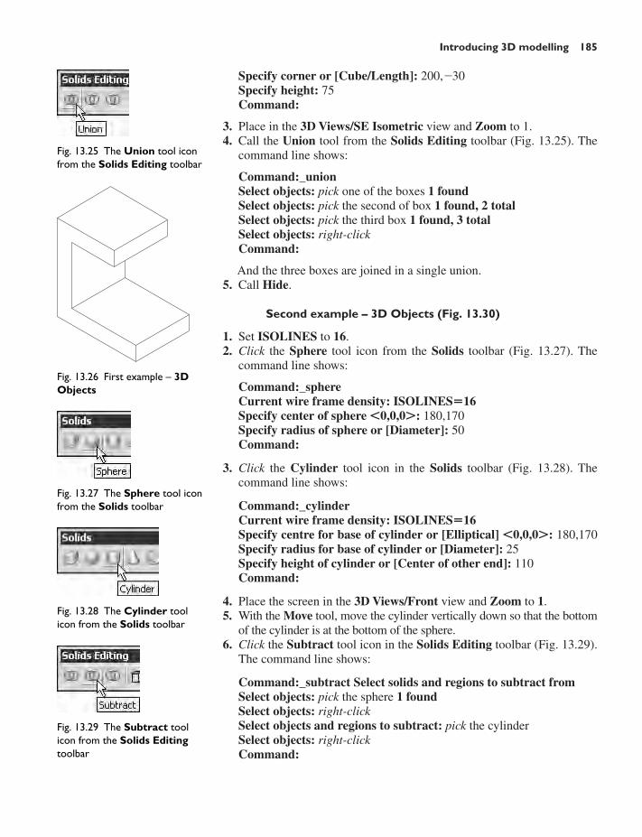
Introducing 3D modelling 185
Specify corner or [Cube/Length]: 200,�30Specify height: 75Command:
3. Place in the 3D Views/SE Isometric view and Zoom to 1.4. Call the Union tool from the Solids Editing toolbar (Fig. 13.25). The
command line shows:
Command:_unionSelect objects: pick one of the boxes 1 foundSelect objects: pick the second of box 1 found, 2 totalSelect objects: pick the third box 1 found, 3 totalSelect objects: right-clickCommand:
And the three boxes are joined in a single union.5. Call Hide.
Second example – 3D Objects (Fig. 13.30)
1. Set ISOLINES to 16.2. Click the Sphere tool icon from the Solids toolbar (Fig. 13.27). The
command line shows:
Command:_sphereCurrent wire frame density: ISOLINES�16Specify center of sphere �0,0,0�: 180,170Specify radius of sphere or [Diameter]: 50Command:
3. Click the Cylinder tool icon in the Solids toolbar (Fig. 13.28). Thecommand line shows:
Command:_cylinderCurrent wire frame density: ISOLINES�16Specify centre for base of cylinder or [Elliptical] �0,0,0�: 180,170Specify radius for base of cylinder or [Diameter]: 25Specify height of cylinder or [Center of other end]: 110Command:
4. Place the screen in the 3D Views/Front view and Zoom to 1.5. With the Move tool, move the cylinder vertically down so that the bottom
of the cylinder is at the bottom of the sphere.6. Click the Subtract tool icon in the Solids Editing toolbar (Fig. 13.29).
The command line shows:
Command:_subtract Select solids and regions to subtract fromSelect objects: pick the sphere 1 foundSelect objects: right-clickSelect objects and regions to subtract: pick the cylinderSelect objects: right-clickCommand:
Fig. 13.25 The Union tool iconfrom the Solids Editing toolbar
Fig. 13.26 First example – 3DObjects
Fig. 13.27 The Sphere tool iconfrom the Solids toolbar
Fig. 13.28 The Cylinder toolicon from the Solids toolbar
Fig. 13.29 The Subtract toolicon from the Solids Editingtoolbar

186 Introduction to AutoCAD 2006
7. Place the screen in the 3D Views/SW Isometric view and Zoom to 1.8. Call Hide.
Third example – 3D Objects (Fig. 13.32)
1. Call the Cylinder tool and with a centre 170,150 construct a cylinderof radius 60 and height 15.
2. Click the Cone tool icon in the Solids toolbar (Fig. 13.31). The commandline shows:
Command:_coneCurrent wire frame density: ISOLINES�16Specify center point for base of cone or [Elliptical]: 170,150Specify radius for base of cone or [Diameter]: 40Specify height of cone or [Apex]: 150Command:
3. Call the Sphere tool and construct a sphere of centre 170,150 andradius 45.
4. Place the screen in the 3D Views/Front view and with the Move tool,move the cone and sphere so that the cone is resting on the cylinderand the centre of the sphere is at the apex of the cone.
5. Place in the 3D Views/SW Isometric view and Zoom to 1 and withUnion form a single 3D model from the three objects.
6. Call Hide.
Fourth example – 3D Objects (Fig. 13.33)
1. Click the Box tool icon in the Solids toolbar and construct two boxes –the first of corners 70,210 and 290,120 and of height 10, the second ofcorners 120,200,10 and 240,130,10 and of height 80.
2. Place the screen in the 3D Views/Front view and Zoom to 1.3. Click the Wedge tool icon in the Solids toolbar. The command line shows:
Command:_wedgeSpecify first corner of wedge or [Center]: 120,170,10Specify corner or [Cube/Length]: 80,160,10Specify height: 70Command: right-clickWEDGESpecify first corner of wedge or [Center]: 240,170,10Specify corner or [Cube/Length]: 280,160,10Specify height: 70Command:
4. Place the screen in the 3D Views/SW Isometric view and Zoom to 10.5. Call the Union tool from the Solids Editing toolbar and in response to
the prompts in the tool’s sequences pick each of the five objects in turnto form a union of the five objects.
6. Call Hide.
Fig. 13.30 Second example – 3DObjects
Fig. 13.31 The Cone tool iconfrom the Solids toolbar
Fig. 13.32 Third example – 3DObjects
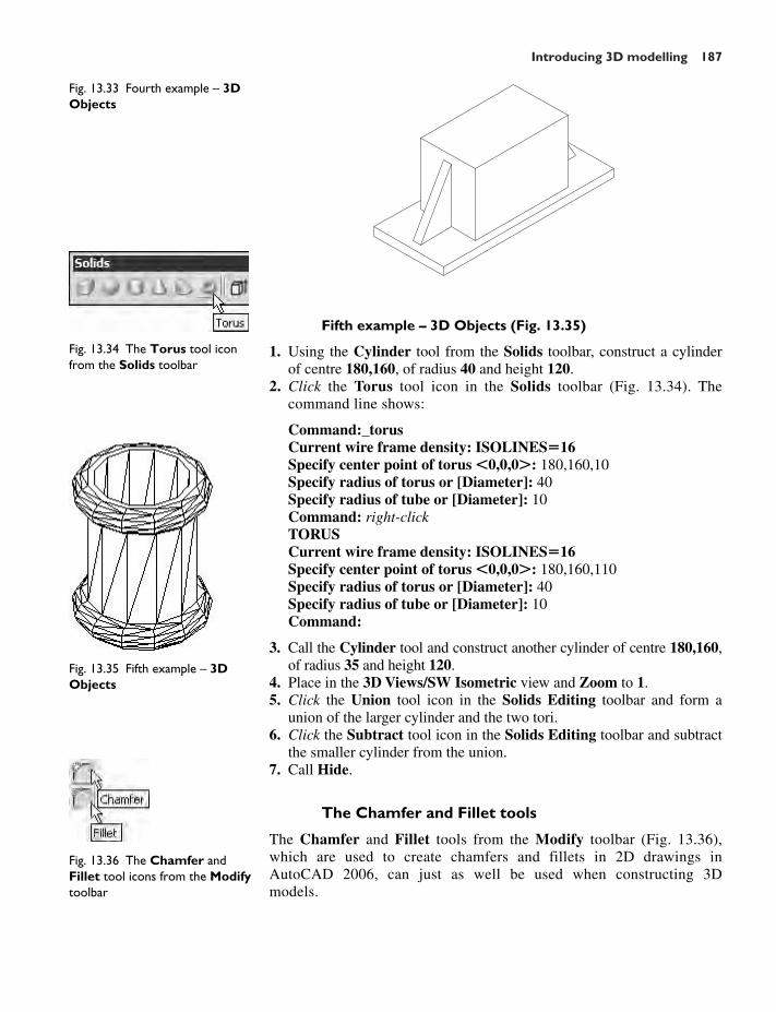
Introducing 3D modelling 187
Fig. 13.33 Fourth example – 3DObjects
Fig. 13.34 The Torus tool iconfrom the Solids toolbar
Fig. 13.35 Fifth example – 3DObjects
Fig. 13.36 The Chamfer andFillet tool icons from the Modifytoolbar
Fifth example – 3D Objects (Fig. 13.35)
1. Using the Cylinder tool from the Solids toolbar, construct a cylinderof centre 180,160, of radius 40 and height 120.
2. Click the Torus tool icon in the Solids toolbar (Fig. 13.34). Thecommand line shows:
Command:_torusCurrent wire frame density: ISOLINES�16Specify center point of torus �0,0,0�: 180,160,10Specify radius of torus or [Diameter]: 40Specify radius of tube or [Diameter]: 10Command: right-clickTORUSCurrent wire frame density: ISOLINES�16Specify center point of torus �0,0,0�: 180,160,110Specify radius of torus or [Diameter]: 40Specify radius of tube or [Diameter]: 10Command:
3. Call the Cylinder tool and construct another cylinder of centre 180,160,of radius 35 and height 120.
4. Place in the 3D Views/SW Isometric view and Zoom to 1.5. Click the Union tool icon in the Solids Editing toolbar and form a
union of the larger cylinder and the two tori.6. Click the Subtract tool icon in the Solids Editing toolbar and subtract
the smaller cylinder from the union.7. Call Hide.
The Chamfer and Fillet tools
The Chamfer and Fillet tools from the Modify toolbar (Fig. 13.36),which are used to create chamfers and fillets in 2D drawings inAutoCAD 2006, can just as well be used when constructing 3Dmodels.

188 Introduction to AutoCAD 2006
Example – Chamfer and Fillet (Fig. 13.39)
1. Using the Box and Cylinder tools, construct the 3D model in Fig. 13.37.2. Place in the 3D Views/SW Isometric view (Fig. 13.38). Union the two
boxes and with the Subtract tool, subtract the cylinders from the union.
Box 160 × 100 × 10 Elliptical cylinder80 × 40 height 60
Cylinders R5height 10
Box 120 × 60 × 50Fig. 13.37 Example – Chamferand Fillet – the model beforeusing the tools
Before chamfersand fillets
Fig. 13.38 Example – isometricview – Chamfer and Fillet –the model before using the tools
Fig. 13.39 Example – Chamferand Fillet
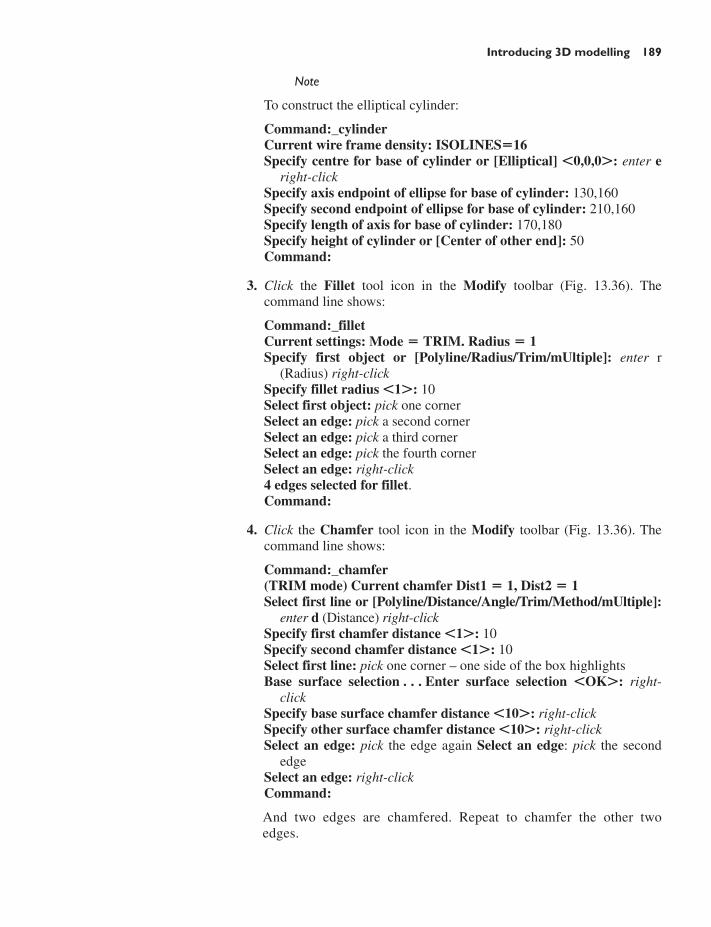
Introducing 3D modelling 189
Note
To construct the elliptical cylinder:
Command:_cylinderCurrent wire frame density: ISOLINES�16Specify centre for base of cylinder or [Elliptical] �0,0,0�: enter e
right-clickSpecify axis endpoint of ellipse for base of cylinder: 130,160Specify second endpoint of ellipse for base of cylinder: 210,160Specify length of axis for base of cylinder: 170,180Specify height of cylinder or [Center of other end]: 50Command:
3. Click the Fillet tool icon in the Modify toolbar (Fig. 13.36). Thecommand line shows:
Command:_filletCurrent settings: Mode � TRIM. Radius � 1Specify first object or [Polyline/Radius/Trim/mUltiple]: enter r
(Radius) right-clickSpecify fillet radius �1�: 10Select first object: pick one cornerSelect an edge: pick a second cornerSelect an edge: pick a third cornerSelect an edge: pick the fourth cornerSelect an edge: right-click4 edges selected for fillet.Command:
4. Click the Chamfer tool icon in the Modify toolbar (Fig. 13.36). Thecommand line shows:
Command:_chamfer(TRIM mode) Current chamfer Dist1 � 1, Dist2 � 1Select first line or [Polyline/Distance/Angle/Trim/Method/mUltiple]:
enter d (Distance) right-clickSpecify first chamfer distance �1�: 10Specify second chamfer distance �1�: 10Select first line: pick one corner – one side of the box highlightsBase surface selection . . . Enter surface selection �OK�: right-
clickSpecify base surface chamfer distance �10�: right-clickSpecify other surface chamfer distance �10�: right-clickSelect an edge: pick the edge again Select an edge: pick the second
edgeSelect an edge: right-clickCommand:
And two edges are chamfered. Repeat to chamfer the other twoedges.

190 Introduction to AutoCAD 2006
Note on the tools Union, Subtract and Intersect
The tools Union, Subtract and Intersect found in the Solids Editingtoolbar are known as the Boolean operators after the mathematicianBoolean. They can be used to form unions, subtractions or intersectionsbetween extrusions, solids of revolution or any of the 3D Objects.
Note on using Modify tools on 3D models
As was seen above when using the Move, Chamfer and Fillet tools fromthe Modify toolbar, so also can other tools from the toolbar be used inconnection with the construction of 3D models. The tools Copy, Mirror,Rotate and Scale from Modify can also be used when constructing 3Dmodels if wished.
Note on rendering
Rendering of 3D models to produce photo-like images will be more fullydescribed in pages 228 to 239. But to give more realism to some of the3D models so far shown in this chapter, try the following for some of themodels which have so far been constructed.
1. Open the file of one of the 3D models so far constructed.2. At the command line:
Command: enter render right-click
And the Render dialog appears (Fig. 13.40). Click its Renderbutton.
Fig. 13.40 The Render dialog

Introducing 3D modelling 191
Note
3D models can be rendered because they are made up from a number of3D meshes. Regions can also be rendered as shown in the renderings ofsome regions constructed earlier in this chapter (Fig. 13.42).
Fig. 13.41 Examples of simplerenderings of 3D models
Fig. 13.42 Examples of renderingsof regions
The model renders to a default set of rendering settings.Examples of renderings of some of the models so far constructed are
shown in Fig. 13.41.

192 Introduction to AutoCAD 2006
Revision notes
1. In the AutoCAD 3D coordinate system, positive Z is towards theoperator away from the monitor screen.
2. A 3D face is a mesh behind which other details can be hidden.3. The Hide tool can be used to hide details behind the 3D meshes of 3D
solid models.4. The Extrude tool can be used for extruding closed plines or regions to
stated heights, to stated slopes or along paths.5. The Revolve tool can be used for constructing solids of revolution
through any angle up to 360�.6. 3D models can be constructed from the 3D objects Box, Sphere, Cylin-
der, Cone, Torus and Wedge. Extrusions and/or solids of revolution mayform part of models constructed using the 3D objects.
7. Tools such as Chamfer and Fillet from the Modify toolbar can beused when constructing 3D models.
8. A simple form of rendering of 3D models can be achieved by enteringrender at the command line followed by a click on the Render buttonof the dialog which appears.
9. The tools Union, Subtract and Intersect are known as the Booleanoperators.
Exercises
The first three exercises given below give practice in the use of the 3DFace and Hide tools. A variety of 3D viewing positions selected fromView/3D Views will need to be used when constructing the 3D modeldrawings in answer to these three exercises.
1. Construct the four steps shown in Fig. 13.43 working to the given sizes.
Each step is 110 longby 30 deep and 30 highFig. 13.43 Exercise 1

Introducing 3D modelling 193
2. Construct the 3D model given in Fig. 13.44 working to the sizes givenwith the drawing.
90°
180Depth is 80
35
35
100
Fig. 13.45 Exercise 3
Main body is 190 × 100 × 75 Cut out portion is 80 × 75 × 50Fig. 13.44 Exercise 2
3. Construct the 3D model drawing of a V block shown in Fig. 13.45working to the sizes given in the right-hand drawing.
The exercises which follow require using the 3D objects tools and thetools Revolve, Extrude, Union and Subtract.
4. Fig. 13.46 shows a rendering of the solid of revolution for this exer-cise. Fig. 13.47 shows the outline from which the solid was obtained.Using the Revolve tool construct the solid of revolution and render theresult.

194 Introduction to AutoCAD 2006
1.5
Scale: 10:1
Axis of revolution
Pline for Revolve of Nozzle
0.5
0.5
0.5
0.5
4
25
3.5
Fig. 13.46 Exercise 4 –a rendering
Fig. 13.47 Exercise 4
45
182
R28
104
78
2
45
Fig. 13.48 Exercise 5 –a rendering
Fig. 13.49 Exercise 5
5. Construct the rendered 3D model of a wine glass as shown in Fig. 13.48,working to the dimensions given in the outline drawing (Fig. 13.49).

Introducing 3D modelling 195
250
110
80 R50
160
Fig. 13.52 Exercise 7
Holes ∅8 R15
R15
R15
150
135
80
80
6
42
12 60
6 50
6
Fig. 13.51 Exercise 6
You will need to construct the outline and change it into a regionbefore being able to change the outline into a solid of revolution usingthe Revolve tool. This is because the semi-elliptical part of the outlinehas been constructed using the Ellipse tool, resulting in part of the out-line being a spline, which cannot be acted upon by Polyline Edit toform a closed pline.
6. Fig. 13.50 is a rendering of the 3D solid model constructed by workingto the information given in Fig. 13.51. Construct the bracket and ren-der as shown in Fig. 13.50.
Fig. 13.50 Exercise 6 – Arendering
7. Working to the dimensions given in Fig. 13.52, construct an extrusionof the plate to a height of 5 units and render as shown in Fig. 13.53.
8. Working to the details given in the orthographic projection in Fig. 13.54,construct a 3D model of the assembly as shown in Fig. 13.55.
After constructing the pline outline(s) required for the solid(s) ofrevolution, use the Revolve tool to form the 3D solid.

196 Introduction to AutoCAD 2006
∅165
∅135
∅110
∅20
∅40
∅30
∅55
A20
1016
0
1020
B
17.5
2.5
R2.510
Detail at A (Scale 2:1)
11.5
R2.5
2.5Detail at B (Scale 2:1)
Fig. 13.54 Exercise 8
Fig. 13.55 Exercise 8 –a rendering
Fig. 13.53 Exercise 7 – arendering

197
CHAPTER 14
3D models in viewports
Aim of this chapter
To give examples of 3D solid models constructed in multiple viewportsettings.
Setting up viewport systems
One of the better methods of constructing 3D models is in differentviewport settings. Working in viewport settings allows what is being con-structed to be seen from a variety of viewing positions. To set up a newviewport system:
1. Click View in the menu bar and from the drop-down menu which appearsclick Viewports and in the sub-menu which then appears click NewViewports . . . (Fig. 14.1). The Viewports dialog appears (Fig. 14.2).
Fig. 14.1 Selecting NewViewports . . . from the Viewdrop-down menu
2. Click the New Viewports tab and a number of named viewports systemsappear in the Standard viewports list in the dialog.
3. Click the name Four: Equal, followed by a click on 3D in the Setuppopup list. A preview of the Four: Equal viewports screen appearsshowing the views appearing in each of the four viewports.

198 Introduction to AutoCAD 2006
4. Click the OK button of the dialog and the AutoCAD 2006 drawingarea appears showing the four viewport layout (Fig. 14.3).
Fig. 14.2 The Viewports dialog
Fig. 14.3 The Four: Equalviewports layout
First example – Four: Equal viewports (Fig. 14.7)
Fig. 14.4 shows a first angle orthographic projection of a support. Toconstruct a Scale 1:1 3D model of the support in a Four: Equal viewportsetting:
1. Click View in the menu bar, followed by a click on Viewports in thedrop-down menu, followed by another click on New Viewports . . . inthe Viewports sub-menu. Make sure the 3D option is selected from theSetup popup list and click the OK button of the dialog. The AutoCAD2006 drawing area appears in a Four: Equal viewport setting.

3D models in viewports 199
Fig. 14.4 Orthographic projectionof the support for the firstexample
Fig. 14.5 The plan view drawn
Dimensions in millimetres
HOLE ∅40
Holes ∅20
30
10
R20
160
DO NOT SCALE
160
30
30
60
20
Name: A. Student Scale: Date: Title:1:1 23.11.2005 Support 45/D
2. Click in the Top viewport (bottom right-hand corner viewport) tomake it current.
3. Set ISOLINES to 4.4. Using the Polyline tool, construct the outline of the plan view of the
plate of the support, including the holes (Fig. 14.5). Note the views inthe other viewports.

200 Introduction to AutoCAD 2006
5. Call the Extrude tool from the Solids toolbar and extrude the planoutline and the circles to a height of 20.
6. With the Subtract tool from the Solids Editing toolbar, subtract theholes from the plate (Fig. 14.6).
7. Call the Box tool and in the centre of the plate construct a box ofWidth � 60, Length � 60 and Height � 30.
8. Call the Cylinder tool and in the centre of the box construct a cylinderof Radius � 20 and Height � 30.
9. Call Subtract and subtract the cylinder from the box.10. Click in the Right viewport. With the Move tool, move the box and
its hole into the correct position with regard to the plate.
Fig. 14.6 The four views afterusing the Extrude and Subtracttools
Fig. 14.7 First example – Four:Equal viewports

3D models in viewports 201
Dimensions in millimetres
30
300
20
DO NOT SCALE
Holes ∅20
Holes ∅80
R15
80 60
R60
R50
R5
10
10
Name: A. Reader Date: Title:Scale: 1:1 12/09/2006 Support Bracket 3/AFig. 14.8 Working drawing for thesecond example
11. With Union, form a union of the plate and box.12. Click in the Front viewport and construct a triangle of one of the
webs attached between the plate and the box. With Extrude, extrudethe triangle to a height of 10. With the Mirror tool, mirror the web tothe other side of the box.
13. Click in the Right viewport and with the Move tool, move the twowebs into their correct position between the box and the plate. Then,with Union, form a union between the webs and the 3D model.
14. While in the Right viewport, construct the other two webs and in theFront viewport, move, mirror and union the webs as in step 13.
Fig. 14.6 shows the resulting four-viewport scene.
Second example – Four: Left viewports (Fig. 14.9)
1. Open the Four: Left viewport layout from the Viewports dialog.2. In the Top viewport construct an outline of the web of the Support
Bracket shown in Fig. 14.8. With the Extrude tool, extrude the partsof the web to a height of 20.
3. With the Subtract tool, subtract the holes from the web.4. While in the Top viewport, construct two cylinders central to the
extrusion – one of radius 50 and height 30, the second of radius 40 andheight 30. With the Subtract tool, subtract the smaller cylinder fromthe larger.
5. Click in the Front viewport and move the cylinders vertically upwardsby 5 units. Then with Union form a union between the cylinders andthe web.
6. Make the Front viewport active and at one end of the union, constructtwo cylinders – the first of radius 10 and height 80, the second ofradius 15 and height 80. Subtract the smaller from the larger.

202 Introduction to AutoCAD 2006
7. With the Mirror tool, mirror the cylinders to the other end of the union.8. Make the Top viewport current and with the Move tool, move the
cylinders to their correct position at the ends of the union. Form a unionbetween all parts on screen.
9. Make the SE Isometric viewport current and enter render at thecommand line, followed by a click on the Render button in the dialogwhich appears.
Fig. 14.9 shows the result.
35
Chamfer 20 × 2025 5
30
340
5 55
65
20
100
Fig. 14.10 Third example –outline for solid of revolution
Fig. 14.9 Second example – Four:Left viewports
Third example – Three: Right viewports (Fig. 14.11)
1. Open the Three: Right viewport layout from the Viewports dialog.Make sure the 3D setup is chosen.
2. Click in the Top viewport (top left-hand viewport) and change it to a3D Views/Right view from the View drop-down menu.
3. In what is now the Right viewport construct a pline outline to thedimensions in Fig. 14.10.

3D models in viewports 203
4. Call the Revolve tool from the Solids toolbar and revolve the outlinethrough 360°.
5. Make the SE Isometric viewport current and render the view (Fig. 14.11).
Fig. 14.11 Third example –Three: Right viewports
Notes
1. When working in viewport layouts such as in the above three examples,it is important to make good use of the Zoom tool, mainly because theviewports are smaller than the whole screen viewport when working inAutoCAD 2006 as a single viewport.
2. As in all other forms of constructing drawings in AutoCAD 2006,frequent toggling of SNAP, ORTHO and GRID will allow speedierand more accurate working.
Revision notes
1. Outlines suitable for use when constructing 3D models can be con-structed using the 2D tools such as Line, Arc, Circle and Polyline.Such outlines must be changed to either closed polylines or regionsbefore being incorporated in 3D models.
2. The use of multiple viewports can be of value when constructing 3Dmodels in that various views of the model appear enabling the operatorto check the accuracy of the 3D appearance throughout the constructionperiod.
Exercises
1. Using the Cylinder, Box, Sphere, Wedge and Fillet tools, together withthe Union and Subtract tools and working to any sizes thought suitable,construct the ‘head’ in the Three: Left viewport as shown in Fig. 14.12.
2. Using the tools Sphere, Box, Union and Subtract and working to thedimensions given in Fig. 14.14, construct the 3D solid model as shownin the rendering in Fig. 14.13.
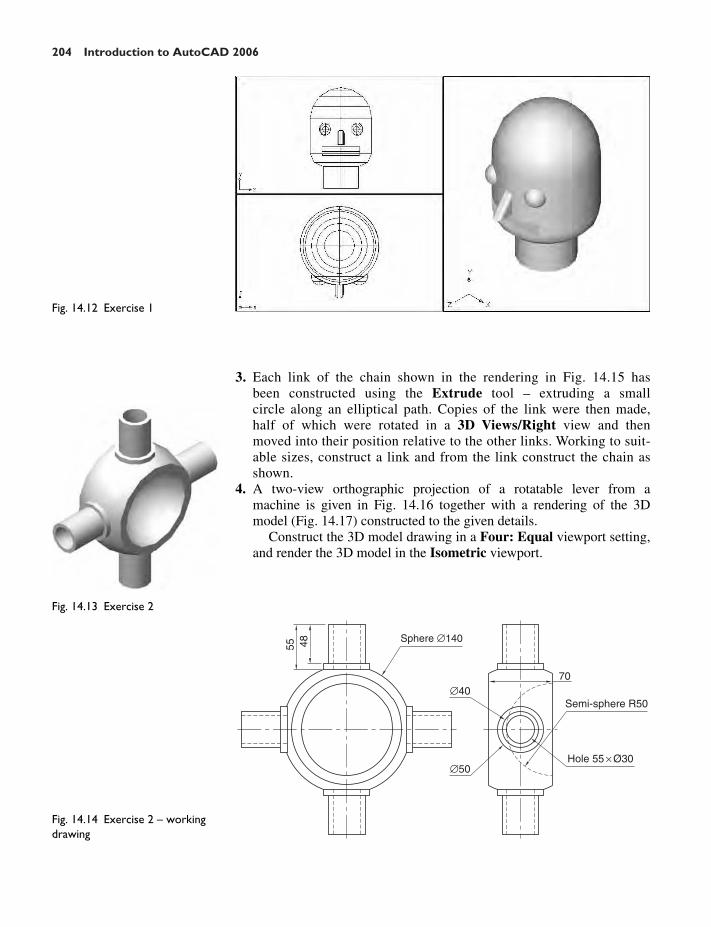
204 Introduction to AutoCAD 2006
Sphere ∅140
∅40
∅50Hole 55 × Ø30
4855
70
Semi-sphere R50
Fig. 14.14 Exercise 2 – workingdrawing
Fig. 14.13 Exercise 2
Fig. 14.12 Exercise 1
3. Each link of the chain shown in the rendering in Fig. 14.15 hasbeen constructed using the Extrude tool – extruding a smallcircle along an elliptical path. Copies of the link were then made,half of which were rotated in a 3D Views/Right view and thenmoved into their position relative to the other links. Working to suit-able sizes, construct a link and from the link construct the chain asshown.
4. A two-view orthographic projection of a rotatable lever from amachine is given in Fig. 14.16 together with a rendering of the 3Dmodel (Fig. 14.17) constructed to the given details.
Construct the 3D model drawing in a Four: Equal viewport setting,and render the 3D model in the Isometric viewport.
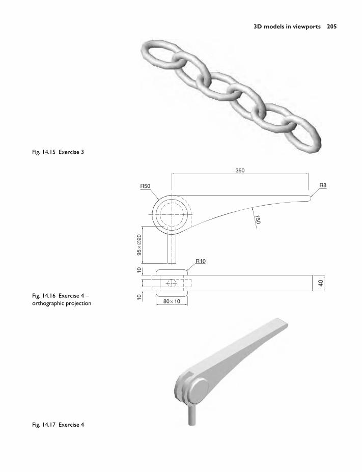
3D models in viewports 205
Fig. 14.15 Exercise 3
R50
350
R8
750
95 ×
∅20
R10
1010 80 × 10
40
Fig. 14.16 Exercise 4 –orthographic projection
Fig. 14.17 Exercise 4

206 Introduction to AutoCAD 2006
Fig. 14.19 Exercise 5
Dimensions in millimetres
Keyway 9 × 9
Hole ∅40
Hole SQ 9
R4
∅180
∅150
∅105
∅60
M.Y.Name Scale 1:1 27/05/2006 FACEPLATE 7/FC
1123
Fig. 14.18 Exercise 5 – dimensions
5. Working in a Three: Left viewport setting, construct a 3D model of thefaceplate to the dimensions given in Fig. 14.18. With the Mirror tool,mirror the model to obtain an opposite facing model. In the Isometricviewport call the Hide tool (Fig. 14.19).
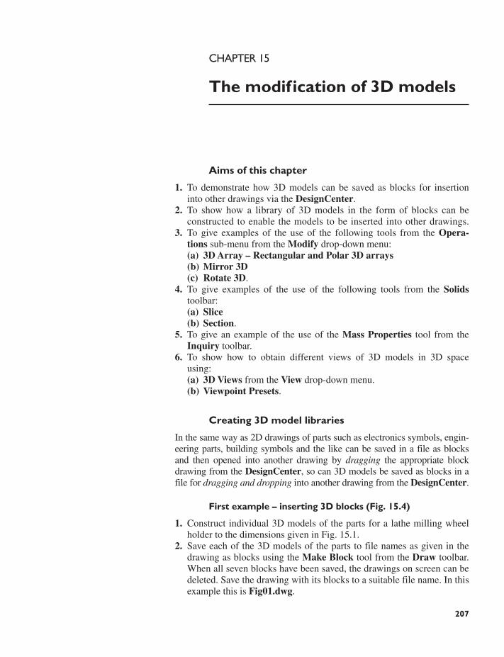
207
CHAPTER 15
The modification of 3D models
Aims of this chapter
1. To demonstrate how 3D models can be saved as blocks for insertioninto other drawings via the DesignCenter.
2. To show how a library of 3D models in the form of blocks can beconstructed to enable the models to be inserted into other drawings.
3. To give examples of the use of the following tools from the Opera-tions sub-menu from the Modify drop-down menu:(a) 3D Array – Rectangular and Polar 3D arrays(b) Mirror 3D(c) Rotate 3D.
4. To give examples of the use of the following tools from the Solidstoolbar:(a) Slice(b) Section.
5. To give an example of the use of the Mass Properties tool from theInquiry toolbar.
6. To show how to obtain different views of 3D models in 3D spaceusing:(a) 3D Views from the View drop-down menu.(b) Viewpoint Presets.
Creating 3D model libraries
In the same way as 2D drawings of parts such as electronics symbols, engin-eering parts, building symbols and the like can be saved in a file as blocksand then opened into another drawing by dragging the appropriate blockdrawing from the DesignCenter, so can 3D models be saved as blocks in afile for dragging and dropping into another drawing from the DesignCenter.
First example – inserting 3D blocks (Fig. 15.4)
1. Construct individual 3D models of the parts for a lathe milling wheelholder to the dimensions given in Fig. 15.1.
2. Save each of the 3D models of the parts to file names as given in thedrawing as blocks using the Make Block tool from the Draw toolbar.When all seven blocks have been saved, the drawings on screen can bedeleted. Save the drawing with its blocks to a suitable file name. In thisexample this is Fig01.dwg.

208 Introduction to AutoCAD 2006
3. Set up a Four: Equal viewports setting.4. Open the DesignCenter with a click on its tool icon in the Standard
toolbar (Fig. 15.2), or by pressing the Ctrl and 2 keys of the keyboard.5. In the DesignCenter click the directory Chapter15, followed by
another click on Fig01.dwg and yet another click on Blocks. The savedblocks appear as icons in the right-hand area of the DesignCenter.
6. Drag and drop the blocks one by one into one of the viewports onscreen. Fig. 15.3 shows the Nut block ready to be dragged into pos-ition in the Front viewport. As the blocks are dropped on screen, theywill need moving into their correct positions in relation to other partsof the assembly by using the Move tool from the Modify toolbar insuitable viewports.
Nut 15 × ∅25tapped M8 × 1.25
Flat 12 × 5
Washers 20 × R9with hole ∅8
Arms (2) 60 × 20 × 15
20
10
Holes ∅6
T-Bar 90 × 47 × 10
M8
Screw75 × ∅8
Pins (2)20 × ∅6
Fig. 15.1 The components of alathe milling wheel holder
Fig. 15.2 Calling theDesignCenter to screen
Fig. 15.3 First example –inserting 3D blocks
7. Using the Move tool, move the individual 3D models into their finalplaces on screen and render the SE Isometric viewport (Fig. 15.4).

The modification of 3D models 209
Notes
1. It does not matter which of the four viewports any one of the blocks isdragged and dropped into. The part automatically assumes the view ofthe viewport.
2. If a block destined for layer 0 is dragged and dropped into the layerCentre (which in our acadiso.dwt is of colour red and of linetypeCENTER2), the block will take on the colour (red) and linetype ofthat layer (CENTER2).
4. As a block is being dragged and dropped from the DesignCenter, thecommand line shows:
Command: DROPGEOM GROUP
5. In this example, the blocks are 3D models and there is no need to usethe Explode tool option.
Second example – a library of fastenings (Fig. 15.6)
1. Construct a number of engineering fastenings. The number con-structed does not matter. In this example only five have been con-structed – a 10 mm round head rivet, a 20 mm countersunk headrivet, a cheese head bolt, a countersunk head bolt and a hexagonalhead bolt together with its nut (Fig. 15.5). With the Make Blocktool save each separately as a block, erase the original drawings andsave the file to a suitable file name – in this example this isFig05.dwg.
2. Open the DesignCenter, click on the Chapter15 directory, followedby a click on Fig05.dwg. Then click again on Blocks in the content listof Fig05.dwg. The five 3D models of fastenings appear as icons in theright-hand side of the DesignCenter (Fig. 15.6).
3. Such engineering fastenings can be dragged and dropped intoposition in any engineering drawing where the fastenings are tobe included.
Fig. 15.4 First example –inserting 3D blocks
Fig. 15.5 Second example – thefive fastenings
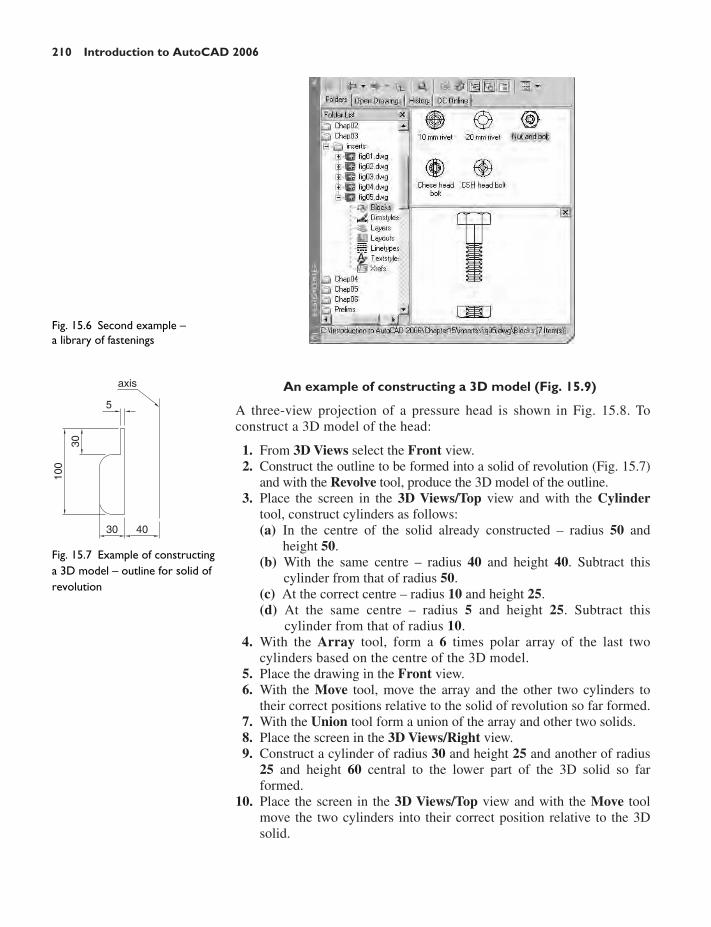
210 Introduction to AutoCAD 2006
An example of constructing a 3D model (Fig. 15.9)
A three-view projection of a pressure head is shown in Fig. 15.8. Toconstruct a 3D model of the head:
1. From 3D Views select the Front view.2. Construct the outline to be formed into a solid of revolution (Fig. 15.7)
and with the Revolve tool, produce the 3D model of the outline.3. Place the screen in the 3D Views/Top view and with the Cylinder
tool, construct cylinders as follows:(a) In the centre of the solid already constructed – radius 50 and
height 50.(b) With the same centre – radius 40 and height 40. Subtract this
cylinder from that of radius 50.(c) At the correct centre – radius 10 and height 25.(d) At the same centre – radius 5 and height 25. Subtract this
cylinder from that of radius 10.4. With the Array tool, form a 6 times polar array of the last two
cylinders based on the centre of the 3D model.5. Place the drawing in the Front view.6. With the Move tool, move the array and the other two cylinders to
their correct positions relative to the solid of revolution so far formed.7. With the Union tool form a union of the array and other two solids.8. Place the screen in the 3D Views/Right view.9. Construct a cylinder of radius 30 and height 25 and another of radius
25 and height 60 central to the lower part of the 3D solid so farformed.
10. Place the screen in the 3D Views/Top view and with the Move toolmove the two cylinders into their correct position relative to the 3Dsolid.
Fig. 15.6 Second example – a library of fastenings
axis
5
30
100
4030
Fig. 15.7 Example of constructinga 3D model – outline for solid ofrevolution

The modification of 3D models 211
11. With Union, form a union between the radius 30 cylinder and the 3Dmodel and with Subtract, subtract the radius 25 cylinder from the 3Dmodel.
12. Call Render and render the model (Fig. 15.9).
Note
This 3D model could equally as well have been constructed in a three orfour viewports setting.
The 3D Array tool
First example – Rectangular array (Fig. 15.12)
1. Construct the star-shaped pline (Fig. 15.10) and extrude it to a heightof 20.
2. Click on Modify in the menu bar and in the drop-down menu whichappears click on 3D Operation, followed by another click on 3D Arrayin the sub-menu which appears (Fig. 15.11). The command line shows:
Command:_3darraySelect objects: pick the extrusion 1 foundSelect objects: right-clickEnter the type of array [Rectangular/Polar] �R�: right-clickEnter the number of rows (—) �1�: enter 3 right-clickEnter the number of columns (III): enter 3 right-clickEnter the number of levels (. . .): enter 4 right-click
R50 Hole ∅80
Holes ∅10
Hole ∅50
∅140
∅60
∅110
∅90
9025
3070
R10
R15
Fig. 15.8 Orthographic drawingfor the example of constructing a3D model
Fig. 15.9 Example of constructinga 3D model
Fig. 15.10 Example – 3DArray – the star pline
70

212 Introduction to AutoCAD 2006
Specify the distance between rows (—): 50Specify the distance between columns (III): 50Specify the distance between levels (. . .): 150Command:
Fig. 15.11 Selecting 3D Arrayfrom the Modify drop-downmenu
3. Place the screen in the 3D Views/SW Isometric view.4. Call the Hide tool.
Second example – Polar array (Fig. 15.13)
1. Use the same star-shaped 3D model.2. Call the 3D Array tool again. The command line shows:
Command:_3darraySelect objects: pick the extrusion 1 foundSelect objects: right-clickEnter the type of array [Rectangular/Polar] �R�: enter p (Polar)
right-clickEnter number of items in the array: 12Specify the angle to fill (�� ccw, �� cw) �360�: right-clickRotate arrayed objects? [Yes/No] �Y�: right-clickSpecify center point of array: 235,125Specify second point on axis of rotation: 300,200Command:
3. Place the screen in the 3D Views/SW Isometric view.4. Render the drawing.
Third example – Polar array (Fig. 15.16)
1. Construct a solid of revolution in the form of an arrow to the dimensionsas shown in Fig. 15.14.
2. Make a 12 times polar array around a central point (Fig. 15.15).3. Call the Union tool and form a union of all 12 items in the array.4. Place the screen in the 3D Views/Front view.5. With the Copy tool, copy the union of the 12 arrows in the array as
follows:
Command:_copySelect objects: click at any point on one of the arrows in the union –
the whole union is pickedSpecify base of displacement: pick any point in the unionSpecify second point of displacement: pick the same point – the
copy is on top of the originalCommand:
Fig. 15.12 First example –Rectangular Array

The modification of 3D models 213
6. Call the Rotate tool from the Modify drop-down menu. The commandline shows:
Command:_rotateSelect objects: enter l (for Last) right-clickSelect objects: right-clickSpecify base point: pick the centre of the arraySpecify rotation angle: enter 90 right-clickCommand:
7. Repeat step 6 to rotate the original array through 45� and alsothrough 135�.
8. Place the composite array in the 3D Views/SW Isometric view andrender.
Fig. 15.13 Second example –Polar array
Ø10 Ø20
50 30
Fig. 15.14 Third example – Polararray – the 3D model to bearrayed
Fig. 15.15 Third example – Polararray – the first array
Fig. 15.16 Third example – Polararray

214 Introduction to AutoCAD 2006
Note
In this example the array did not require the use of the 3D Array tool,because all arrays were on objects in the same plane.
The Mirror 3D tool
First example – Mirror 3D (Fig. 15.20)
1. Construct the array of ellipses and circle as shown in Fig. 15.17.2. Change the 11 objects into regions, form a union of the ellipses and
subtract the circle from the ellipses.3. Extrude the region to a height of 5 and render. The rendering in the
SW Isometric view is shown in Fig. 15.18.4. Click on Mirror 3D in the 3D Operation sub-menu of the Modify
drop-down menu (Fig. 15.19). The command line shows:
Command:_mirror3dSelect objects: pick the extrusion 1 foundSelect objects: right-clickSpecify first point on mirror plane (3 points): 80,130,100Specify second point on mirror plane: 170,220,50Specify third point on mirror plane: 180,160,20Delete source objects? [Yes/No] �N�: right-clickCommand:
Ellipse 40 × 10
Arrayed10 times R10
Fig. 15.18 First example –Mirror 3D – the object to bemirrored
Fig. 15.19 Calling Mirror 3D fromthe Modify drop-down menu
Fig. 15.17 First example –Mirror 3D – plan of object tobe mirrored
Fig. 15.20 First example –Mirror 3D

The modification of 3D models 215
Second example – Mirror 3D (Fig. 15.23)
1. Construct a solid of revolution in the shape of a bowl in the 3DViews/Front view (Fig. 15.21).
2. Click Mirror 3D in the 3D Operations sub-menu of the Modifydrop-down menu. The command line shows:
Command:_mirror3dSelect objects: pick the bowl 1 foundSelect objects: right-clickSpecify first point on mirror plane (3 points): pickSpecify second point on mirror plane: pickSpecify third point on mirror plane: enter .xy right-click (need Z):
enter 1 right-clickDelete source objects? [Yes/No] �N�: right-clickCommand:
Note
The line in the illustration shows the top edge of an imaginaryplane vertical to the plane on which the drawing is being constructed(Fig. 15.22).
Second point
First point
Third point.xy and 1
Fig. 15.21 Second example –Mirror 3D – the 3D model
Fig. 15.22 Second example –Mirror 3D – the result in afront view
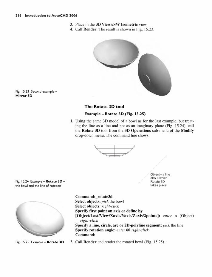
216 Introduction to AutoCAD 2006
3. Place in the 3D Views/SW Isometric view.4. Call Render. The result is shown in Fig. 15.23.
Fig. 15.23 Second example –Mirror 3D
The Rotate 3D tool
Example – Rotate 3D (Fig. 15.25)
1. Using the same 3D model of a bowl as for the last example, but treat-ing the line as a line and not as an imaginary plane (Fig. 15.24), callthe Rotate 3D tool from the 3D Operations sub-menu of the Modifydrop-down menu. The command line shows:
Object – a lineabout whichRotate 3Dtakes place
Fig. 15.24 Example – Rotate 3D –the bowl and the line of rotation
Fig. 15.25 Example – Rotate 3D
Command:_rotate3dSelect objects: pick the bowlSelect objects: right-clickSpecify first point on axis or define by[Object/Last/View/Xaxis/Yaxis/Zaxis/2points]: enter o (Object)
right-clickSpecify a line, circle, arc or 2D-polyline segment: pick the lineSpecify rotation angle: enter 60 right-clickCommand:
2. Call Render and render the rotated bowl (Fig. 15.25).
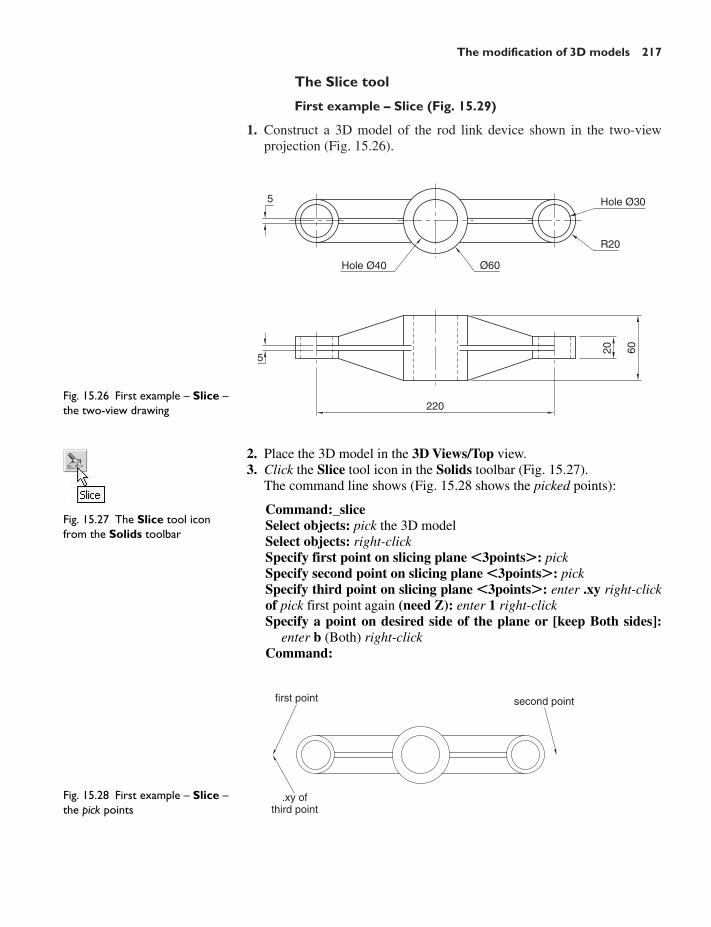
The modification of 3D models 217
The Slice tool
First example – Slice (Fig. 15.29)
1. Construct a 3D model of the rod link device shown in the two-viewprojection (Fig. 15.26).
5
Hole Ø40 Ø60
Hole Ø30
R20
5
220
20 60
Fig. 15.26 First example – Slice –the two-view drawing
2. Place the 3D model in the 3D Views/Top view.3. Click the Slice tool icon in the Solids toolbar (Fig. 15.27).
The command line shows (Fig. 15.28 shows the picked points):
Command:_sliceSelect objects: pick the 3D modelSelect objects: right-clickSpecify first point on slicing plane �3points�: pickSpecify second point on slicing plane �3points�: pickSpecify third point on slicing plane �3points�: enter .xy right-clickof pick first point again (need Z): enter 1 right-clickSpecify a point on desired side of the plane or [keep Both sides]:
enter b (Both) right-clickCommand:
second point
.xy ofthird point
first point
Fig. 15.28 First example – Slice –the pick points
Fig. 15.27 The Slice tool iconfrom the Solids toolbar

218 Introduction to AutoCAD 2006
4. With the Move tool, move the lower half of the sliced model awayfrom the upper half.
5. Place the 3D model(s) in a SW Isometric view.6. Call Render.
The result is shown in Fig. 15.29.
Second example – Slice (Fig. 15.30)
1. Construct the closed pline (Fig. 15.30) and with the Revolve tool, forma solid of revolution from the pline.
Fig. 15.29 First example – Slice
6560
105
15
2
280
R100
R90
40
Fig. 15.30 Second example – Slice
2. With the Slice tool and working to the same sequence as for the firstSlice example, form two halves of the 3D model and render.
The Section tool
First example – Section (Fig. 15.34)
1. Construct a 3D model to the information given in Fig. 15.31 onlayer 0. Note there are three objects in the model – a box, a lid anda cap.
2. Place the model in the 3D Views/Top view.3. Click in the layer field of the Layers toolbar (Fig. 15.32) and click
again on Construction to make it the current layer. Its colour iscyan.
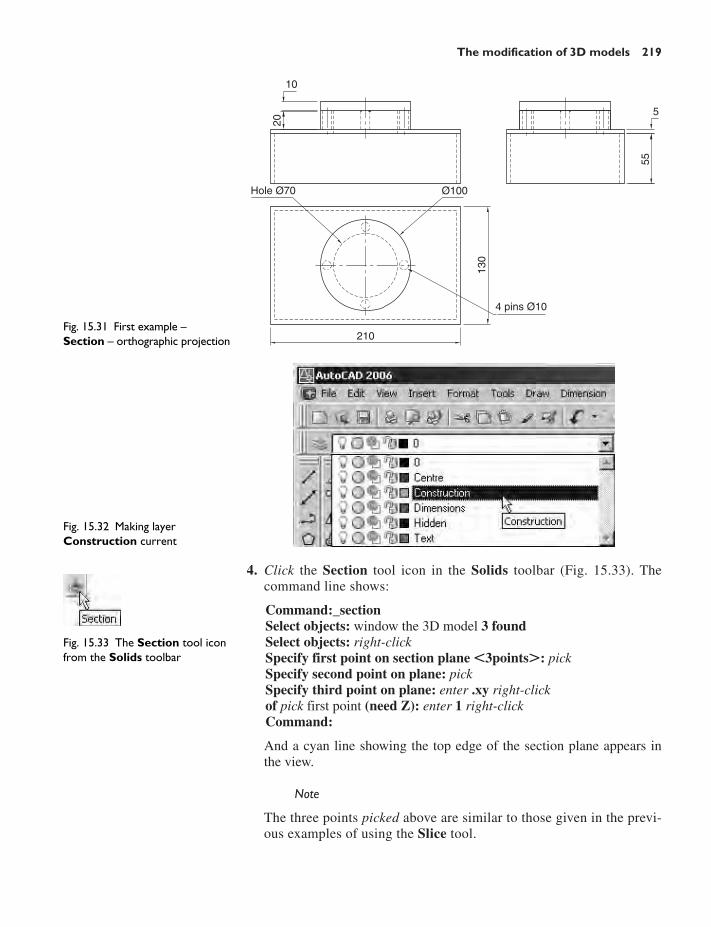
The modification of 3D models 219
4. Click the Section tool icon in the Solids toolbar (Fig. 15.33). Thecommand line shows:
Command:_sectionSelect objects: window the 3D model 3 foundSelect objects: right-clickSpecify first point on section plane �3points�: pickSpecify second point on plane: pickSpecify third point on plane: enter .xy right-clickof pick first point (need Z): enter 1 right-clickCommand:
And a cyan line showing the top edge of the section plane appears inthe view.
Note
The three points picked above are similar to those given in the previ-ous examples of using the Slice tool.
10
20
Hole Ø70 Ø100
130
4 pins Ø10
210
55
5
Fig. 15.33 The Section tool iconfrom the Solids toolbar
Fig. 15.32 Making layerConstruction current
Fig. 15.31 First example –Section – orthographic projection
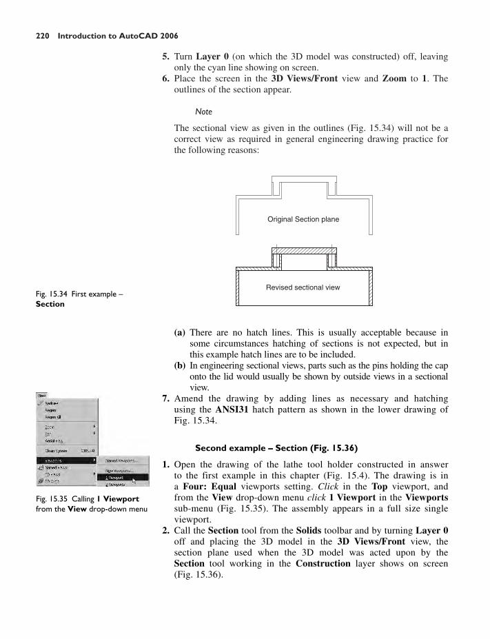
220 Introduction to AutoCAD 2006
5. Turn Layer 0 (on which the 3D model was constructed) off, leavingonly the cyan line showing on screen.
6. Place the screen in the 3D Views/Front view and Zoom to 1. Theoutlines of the section appear.
Note
The sectional view as given in the outlines (Fig. 15.34) will not be acorrect view as required in general engineering drawing practice forthe following reasons:
Original Section plane
Revised sectional viewFig. 15.34 First example –Section
Fig. 15.35 Calling 1 Viewportfrom the View drop-down menu
(a) There are no hatch lines. This is usually acceptable because insome circumstances hatching of sections is not expected, but inthis example hatch lines are to be included.
(b) In engineering sectional views, parts such as the pins holding the caponto the lid would usually be shown by outside views in a sectionalview.
7. Amend the drawing by adding lines as necessary and hatchingusing the ANSI31 hatch pattern as shown in the lower drawing ofFig. 15.34.
Second example – Section (Fig. 15.36)
1. Open the drawing of the lathe tool holder constructed in answerto the first example in this chapter (Fig. 15.4). The drawing is ina Four: Equal viewports setting. Click in the Top viewport, andfrom the View drop-down menu click 1 Viewport in the Viewportssub-menu (Fig. 15.35). The assembly appears in a full size singleviewport.
2. Call the Section tool from the Solids toolbar and by turning Layer 0off and placing the 3D model in the 3D Views/Front view, thesection plane used when the 3D model was acted upon by theSection tool working in the Construction layer shows on screen(Fig. 15.36).

The modification of 3D models 221
The Massprop tool
Example – Massprop (Fig. 15.40)
1. Open the 3D model of the rod link device shown in Fig. 15.26 onpage 217.
2. Call the Mass Properties tool – either with a click on its tool icon inthe Inquiry toolbar (Fig. 15.37) or by entering massprop at thecommand line. When called, the command line shows:
Command:_masspropSelect objects: pick the 3D model 1 foundSelect objects: right-click
An AutoCAD Text Window appears showing the mass properties ofthe picked 3D model (Fig. 15.38).
Fig. 15.36 Second example –Section
Fig. 15.37 The Mass Propertiestool icon in the Inquiry toolbar
Fig. 15.38 Massprop tool. TheAutoCAD Text window showingthe mass properties
Press ENTER to continue:Write analysis to a field [Yes/No]: enter y right-click
And the Create Mass and Area Properties File dialog appearsshowing the name of the file, Fig26_mass.mpr (Fig. 15.39). Click theSave button of the dialog and the file is saved – in this case to the filename Fig26_mass.mpr.
Command:

222 Introduction to AutoCAD 2006
3. Open the application Window Excel (a database program). Click onthe name File in its menu bar, followed by another click on Open . . .and from the Open sub-menu which then appears, select the fileFig26_mass.mpr. The details from the AutoCAD Text Window appearas a database in Excel (Fig. 15.40).
Fig. 15.39 Massprop tool. TheCreate Mass and AreaProperties File dialog
Fig. 15.40 Part of the Exceldatabase file
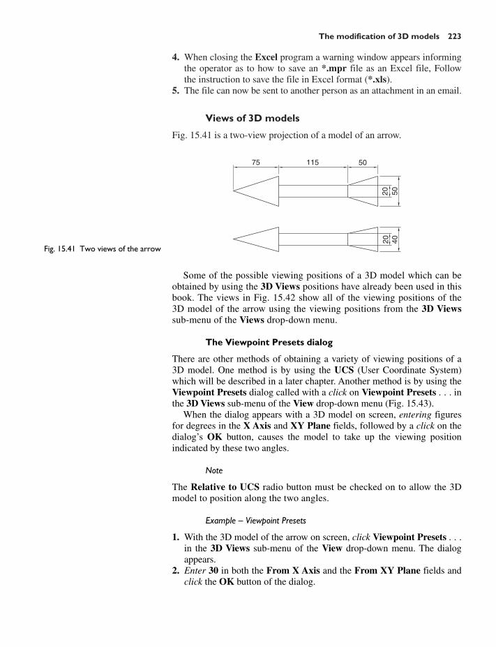
The modification of 3D models 223
4. When closing the Excel program a warning window appears informingthe operator as to how to save an *.mpr file as an Excel file, Followthe instruction to save the file in Excel format (*.xls).
5. The file can now be sent to another person as an attachment in an email.
Views of 3D models
Fig. 15.41 is a two-view projection of a model of an arrow.
75 115 50
20 5020 40
Fig. 15.41 Two views of the arrow
Some of the possible viewing positions of a 3D model which can beobtained by using the 3D Views positions have already been used in thisbook. The views in Fig. 15.42 show all of the viewing positions of the3D model of the arrow using the viewing positions from the 3D Viewssub-menu of the Views drop-down menu.
The Viewpoint Presets dialog
There are other methods of obtaining a variety of viewing positions of a3D model. One method is by using the UCS (User Coordinate System)which will be described in a later chapter. Another method is by using theViewpoint Presets dialog called with a click on Viewpoint Presets . . . inthe 3D Views sub-menu of the View drop-down menu (Fig. 15.43).
When the dialog appears with a 3D model on screen, entering figuresfor degrees in the X Axis and XY Plane fields, followed by a click on thedialog’s OK button, causes the model to take up the viewing positionindicated by these two angles.
Note
The Relative to UCS radio button must be checked on to allow the 3Dmodel to position along the two angles.
Example – Viewpoint Presets
1. With the 3D model of the arrow on screen, click Viewpoint Presets . . .in the 3D Views sub-menu of the View drop-down menu. The dialogappears.
2. Enter 30 in both the From X Axis and the From XY Plane fields andclick the OK button of the dialog.

224 Introduction to AutoCAD 2006
3. The 3D model takes up the viewing position indicated by the twoangles (Fig. 15.44).
Revision notes
1. 3D models can be saved as blocks in a similar manner to the methodof saving 2D drawings as blocks.
2. Libraries can be made up from 3D model drawings.3. 3D models saved as blocks can be inserted into other drawings via
the DesignCenter.4. Arrays of 3D model drawings can be constructed in 3D space using
the 3D Array tool.5. 3D models can be mirrored in 3D space using the Mirror 3D tool.
3D Views / NW Isometric 3D Views / NE Isometric
3D Views / SW Isometric
3D Views / SE Isometric
3D Views / Front 3D Views / Back
3D Views / Left 3D Views / Right
3D Views / Top 3D Views / Bottom
Fig. 15.42 The views from 3DViews
Fig. 15.43 Calling the ViewpointPresets dialog
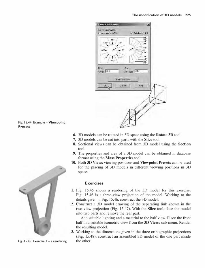
The modification of 3D models 225
Fig. 15.44 Example – ViewpointPresets
6. 3D models can be rotated in 3D space using the Rotate 3D tool.7. 3D models can be cut into parts with the Slice tool.8. Sectional views can be obtained from 3D model using the Section
tool.9. The properties and area of a 3D model can be obtained in database
format using the Mass Properties tool.10. Both 3D Views viewing positions and Viewpoint Presets can be used
for the placing of 3D models in different viewing positions in 3Dspace.
Exercises
1. Fig. 15.45 shows a rendering of the 3D model for this exercise.Fig. 15.46 is a three-view projection of the model. Working to thedetails given in Fig. 15.46, construct the 3D model.
2. Construct a 3D model drawing of the separating link shown in thetwo-view projection (Fig. 15.47). With the Slice tool, slice the modelinto two parts and remove the rear part.
Add suitable lighting and a material to the half view. Place the fronthalf in a suitable isometric view from the 3D Views sub-menu. Renderthe resulting model.
3. Working to the dimensions given in the three orthographic projections(Fig. 15.48), construct an assembled 3D model of the one part insidethe other.Fig. 15.45 Exercise 1 – a rendering

226 Introduction to AutoCAD 2006
With the Slice tool, slice the resulting 3D model into two equalparts, place in an isometric view and call the Hide tool as indicated inFig. 15.49.
4. Construct a solid of revolution of the jug shown in the orthographicprojection (Fig. 15.50). Construct a handle from an extrusion of a circlealong a semicircular path. Union the two parts.
Place the resulting model in the 3D Views/Plan view and add lighting.Also add a suitable glass material.
Place the 3D model in a suitable isometric view and render.
Ø80
R5
R5
R50
Holes Ø20
40
R45
200
10
100
3015
Fig. 15.47 Exercise 2
130
25
Holes Ø6
1005
125
Hole Ø20R2015
R10
R5
15
Fig. 15.46 Exercise 1 – three-viewprojection

The modification of 3D models 227
Ø180
Ø40
Ø50Ø50
Ø40
R120
2
180
55
1011
5
210
5
245
Fig. 15.48 Exercise 3 –orthographic projections
Torus R67.5 tube R2.5
Torus R70 tube R5Cylinder R65 and 245 high
Cylinder R70 and 250 high
R58
R72
Torus R50 tube R7
10
250
245
Fig. 15.49 Exercise 3
Fig. 15.50 Exercise 4

CHAPTER 16
Rendering
Aims of this chapter
1. To introduce the use of the Render tools in producing photographiclike images of 3D solid models.
2. To show how to illuminate a 3D solid model to obtain good lightingeffects when rendering.
3. To give examples of the rendering of 3D solid models.4. To introduce the idea of adding materials to 3D solid models in order
to obtain a realistic appearance to a rendering.5. To demonstrate the use of the forms of shading available using the 3D
Orbit tool.6. To demonstrate methods of printing rendered 3D solid models.
The Render tools
The use of the Render tool has already been shown in examples inprevious pages. More realistic images can be produced using the tool,if lights, colours and/or materials are added to the 3D model beingrendered. All the tools in the Render toolbar have already been shownon page 174.
Render lights
There are four types of lights available when using AutoCAD – Ambientlights, Point lights, Distant lights and Spotlights.
Ambient lighting is taken as the general overall light that is all aroundand surrounding any object. When rendering in AutoCAD Ambient lightis generally set at a default value of 0.3.
Point lights shed light in all directions from the position in which thelight is placed and diminishes in intensity the further from the light thatan object is placed.
Distant lights send parallel rays of light from their position in thedirection chosen by the operator. There is no diminution of the lightintensity no matter how far from an object the lights are placed.
Spotlights illuminate as if from a spotlight. The light is in a direction setby the operator and is in the form of a cone, with a ‘hotspot’ cone givinga brighter spot on the model being lit.
228

Rendering 229
Placing lights to illuminate a 3D model
Any number of the three types of lights – Point, Distant and Spotlightcan be positioned in 3D space as wished by the operator.
In general reasonably good lighting effects can be obtained by placinga Point light high above the object(s) being illuminated, with a Distantlight placed pointing towards the object at a distance from the front andabove the general height of the object(s) and with a second Distant lightpointing towards the object(s) from one side and not as high as the firstDistant light. If desired Spotlights can be used either on their own or inconjunction with the other two forms of lighting. Ambient light is auto-matically placed in the 3D space occupied by the model and other lightingwhen any form of lighting is added to a scene.
First example – rendering a 3D model (Fig. 16.5)
1. Construct a 3D model of the wing nut shown in the two-view projectionin Fig. 16.1.
Ø6010
Tapped M45
6535
20R2
140
20
R10115
60
Fig. 16.1 First example –Rendering – two-viewprojection
2. Place the 3D model in the 3D Views/Top view, Zoom to 1 and withthe Move tool, move the model to the upper part of the AutoCADdrawing area.
3. Click on the Lights tool icon in the Render toolbar (Fig. 16.2). TheLights dialog appears (Fig. 16.3).
4. In the dialog click on the New . . . button to the left of the field read-ing Point Light. The dialog is replaced by the New Point Lightdialog (Fig. 16.4).
Fig. 16.2 The Lights tool icon inthe Render toolbar
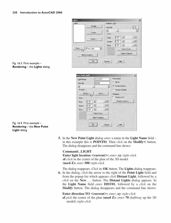
230 Introduction to AutoCAD 2006
5. In the New Point Light dialog enter a name in the Light Name field –in this example this is POINT01. Then click on the Modify� button.The dialog disappears and the command line shows:
Command:_LIGHTEnter light location �current�: enter .xy right-clickof click in the centre of the plan of the 3D model(need Z): enter 500 right-click
The dialog reappears. Click its OK button. The Lights dialog reappears.6. In the dialog, click the arrow to the right of the Point Light field and
from the popup list which appears click Distant Light, followed by aclick on the New . . . button. The Distant Lights dialog appears. Inthe Light Name field enter DIST01, followed by a click on theModify button. The dialog disappears and the command line shows:
Enter direction TO �current�: enter .xy right-clickof pick the centre of the plan (need Z): enter 70 (halfway up the 3D
model) right-click
Fig. 16.3 First example –Rendering – the Lights dialog
Fig. 16.4 First example –Rendering – the New PointLight dialog

Rendering 231
Enter light direction FROM �current�: enter .xy right-clickof enter 150,�20 right-click (need Z): enter 500 right-click
And the dialog reappears.7. Modify another Distant Light to the same position from �80,�20,300.8. Click the OK button of the dialog. It is replaced by the Lights dialog.
Click its OK button.9. Place the model in the 3D View/SW Isometric view, Zoom
window the drawing to a suitable size and click the Render buttonin the Render toolbar. In the dialog which appears click theRender button. The model renders, but will probably be far toobrightly lit.
10. Go back to the Lights dialog and select any one of the light names inthe Lights list and in the appropriate light dialog, alter the Intensityof the light by moving the Intensity slider by dragging with themouse. It will probably be necessary to lessen the light intensity ofeach of the three lights in this manner.
11. Now render again. If necessary again alter the light intensity of thelights until satisfied.
The resulting rendering is shown in Fig. 16.5.
Adding materials to a model
1. Click on the Materials Library tool icon in the Render toolbar(Fig. 16.6). The Materials Library dialog appears (Fig. 16.7).
Fig. 16.6 The Materials Librarytool icon in the Render toolbar
Fig. 16.7 Rendering – theMaterials Library dialog
2. In the dialog click BRASS GIFMAP in the Current Library list,followed by a click on the Preview button.
3. If satisfied with the preview, click the Import button. The nameBRASS GIFMAP appears in the Current Drawing list.
4. Click the dialog’s OK button.
Fig. 16.5 First example –Rendering

232 Introduction to AutoCAD 2006
5. Click on the Materials tool icon in the Render toolbar. The Materialsdialog appears showing BRASS GIFMAP highlighted in its Materialslist. Click the dialog’s Attach button. The dialog disappears. Click onthe 3D model to attach the brass material to the model and when thedialog reappears, click its OK button.
6. The 3D model can now be rendered again. It will be seen that themodel appears as if made in brass.
Notes
1. In each of the Lights dialogs there is a check box by which Shadowscan be switched on. However note that the check box under RenderingOptions in the Render dialog must also be on.
2. The limited descriptions of rendering given in these pages do not showthe full value of different types of lights, materials and renderingmethods. The reader is advised to experiment with the facilities avail-able for rendering.
Second example – rendering a 3D model (Fig. 16.9)
1. Construct 3D models of the two parts of the stand and supportgiven in the projections in Fig. 16.8 with the two parts assembledtogether.
R45
R40
300
Holes Ø8 Ø80
130
5
15
100
15165
15
100
10
Holes Ø10
10 60 15 R50
5
70 20
20
170
Fig. 16.8 Second example –Rendering – projections of thetwo parts
2. Place the scene in the 3D Views/Top view and add lighting.3. Add the two materials BRASS VALLEY and METAL CHERRY
RED to the parts of the assembly and render the result.
Fig. 16.9 shows the resulting rendering.Fig. 16.9 Second example –Rendering

Rendering 233
The 3D Orbit toolbar
Bring the 3D Orbit toolbar on screen from the toolbar menu (right-clickin any toolbar on screen) – Fig. 16.10. Only one of the tools will beshown in an example in this book – the 3D Orbit tool, but it is advisableto practise using other tools in the toolbar to understand how 3D modelscan be manipulated by using the tools in this toolbar.
Fig. 16.10 The 3D Orbit toolbar
Example – 3D Orbit (Fig. 16.11)
This is another tool for the manipulation of 3D models into differentpositions within 3D space.
1. Open the file of the second example of rendering (Fig. 16.9).2. Click on the 3D Orbit tool in the 3D Orbit toolbar. A coloured circle
appears central to the screen with small circles at its quadrants. Thecursor appears as a small black circle (if outside the main circle), asan icon formed from two crossing ellipses (if inside the main circle)and as an ellipse if inside one of the smaller circles at the quadrant(Fig. 16.11).
Fig. 16.11 Example – 3D Orbit
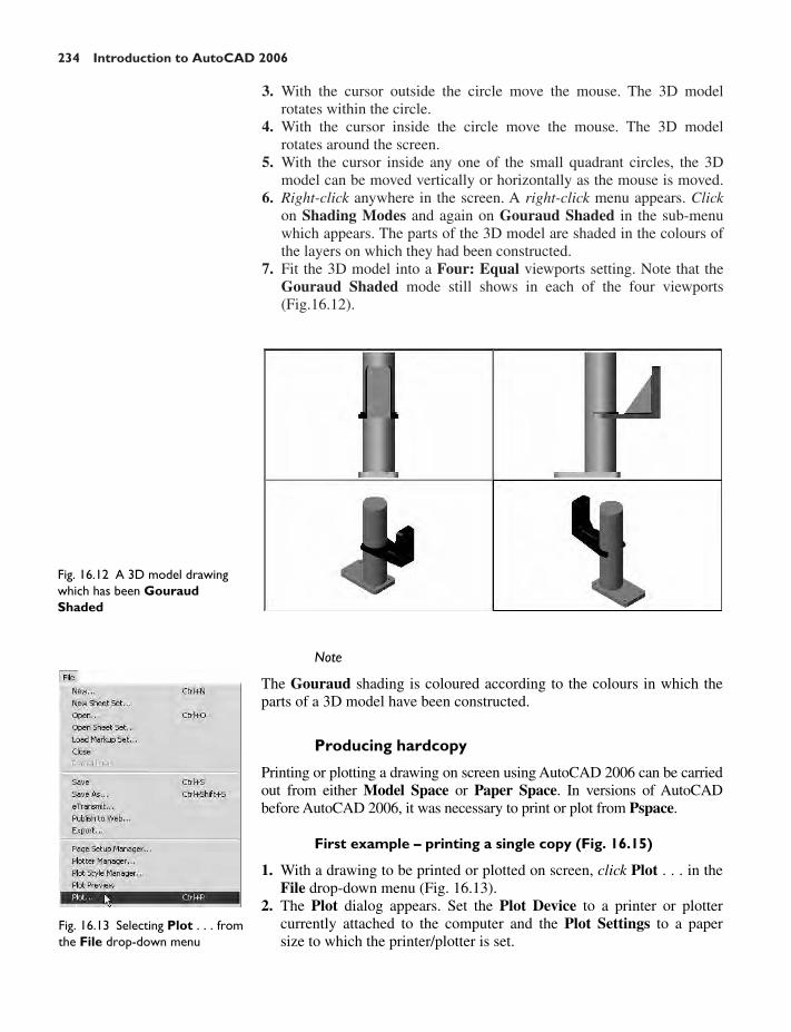
234 Introduction to AutoCAD 2006
3. With the cursor outside the circle move the mouse. The 3D modelrotates within the circle.
4. With the cursor inside the circle move the mouse. The 3D modelrotates around the screen.
5. With the cursor inside any one of the small quadrant circles, the 3Dmodel can be moved vertically or horizontally as the mouse is moved.
6. Right-click anywhere in the screen. A right-click menu appears. Clickon Shading Modes and again on Gouraud Shaded in the sub-menuwhich appears. The parts of the 3D model are shaded in the colours ofthe layers on which they had been constructed.
7. Fit the 3D model into a Four: Equal viewports setting. Note that theGouraud Shaded mode still shows in each of the four viewports(Fig.16.12).
Fig. 16.12 A 3D model drawingwhich has been GouraudShaded
Fig. 16.13 Selecting Plot . . . fromthe File drop-down menu
Note
The Gouraud shading is coloured according to the colours in which theparts of a 3D model have been constructed.
Producing hardcopy
Printing or plotting a drawing on screen using AutoCAD 2006 can be carriedout from either Model Space or Paper Space. In versions of AutoCADbefore AutoCAD 2006, it was necessary to print or plot from Pspace.
First example – printing a single copy (Fig. 16.15)
1. With a drawing to be printed or plotted on screen, click Plot . . . in theFile drop-down menu (Fig. 16.13).
2. The Plot dialog appears. Set the Plot Device to a printer or plottercurrently attached to the computer and the Plot Settings to a papersize to which the printer/plotter is set.

Rendering 235
3. Click the Preview button of the dialog and if the preview is OK, right-click and in the right-click menu which appears, click Plot (Fig. 16.14).The drawing plots producing the necessary ‘hardcopy’ (Fig. 16.15).
Fig. 16.14 The right-click menu inthe print Preview window
Fig. 16.15 First example –printing a single copy
Second example – multiple view copy (Fig. 16.16)
A 3D model to be printed is a Gouraud Shaded 3D model which hasbeen constructed on three layers – Red, Blue and Green in colour. Toprint a multiple view copy:
1. Place the drawing in a Four: Equal viewport setting.2. Make a new layer vports of colour cyan and make it the current layer.3. Click the Layout1 tab. The drawing appears in Pspace with the Page
Setup – Layout1 dialog on top.4. Make sure the Plot Device and Plot Settings are correct and click the
OK button of the dialog.5. A view of the 3D model appears within a cyan coloured viewport.
With the Erase tool erase the viewport. The drawing is erased.6. At the command line:
Command: enter mv (MVIEW) right-clickSpecify corner of viewport or [ON/OFF/Fit/Shadeplot/Lock/
Object/Polygonal/Restore/2/3/4] �Fit�: enter 4 right-clickSpecify first corner or [Fit] �Fit�: right-click
And a four-viewport layout appears in Paper Space (Fig. 16.17).7. Click the PAPER button in the status bar. It changes to MODEL.8. Set the viewports to suitable 3D View settings.9. Click Plot . . . in the File drop-down menu and when the Plot dialog
appears, click its Full Preview button.10. If the preview is satisfactory (Fig. 16.17), right-click and from the
right-click menu click Plot. The drawing plots to produce therequired four-viewport hardcopy.

236 Introduction to AutoCAD 2006
Other forms of hardcopy
When working in AutoCAD 2006, several different forms of hardcopy canbe printed or plotted determined by the settings in the 3D Orbit/ShadingModes settings (Fig. 16.18). As an example a single view plot review ofthe same 3D model is shown in the Hidden shading form (Fig. 16.19).
Saving and opening 3D model drawings
3D model drawings are saved and/or opened in the same way as are 2D draw-ings. To save a drawing click Save As . . . in the File drop-down menu and in
Fig. 16.16 Second example –multiple view copy
Fig. 16.17 Second example –multiple view copy – a printPreview

Rendering 237
Fig. 16.19 An example of Hiddenshading plot Preview
the Save Drawing As dialog which appears enter a file name in the FileName field of the dialog before clicking the Save button. To open a drawingwhich has been saved click Open . . . in the File drop-down menu, and in theSelect File dialog which appears select a file name form the file list.
There are differences between saving a 2D and a 3D drawing, in thatwhen 3D model drawing is shaded by using a shading mode from the3D Orbit/Shading Modes sub-menu, the shading is saved with thedrawing.
Exercises
1. A rendering of an assembled lathe tool holder is shown in Fig. 16.20.The rendering includes different materials for each part of the assembly.
Working to the dimensions given in the parts orthographic drawing(Fig. 16.21), construct a 3D model drawing of the assembled lathetool holder on several layers of different colours and shade using the3D Orbit/Gouraud shading method. Add lighting and materials andrender the model in an isometric view.
2. Working to the sizes given in the two-view orthographic projection inFig. 16.22, construct a 3D model drawing of the drip tray from anengine. Add lighting and the material OLIVE METAL, place themodel in an isometric view and render (Fig. 16.23).
Fig. 16.18 The 3D Orbit/ShadingModes settings menu

238 Introduction to AutoCAD 2006
Fig. 16.20 Exercise 1 – arendering
160 × Ø12
11
Hole Ø8 C'boreØ18 × 1 deep
9020
115R4
4
203230
R15
R4
45
Fig. 16.21 Exercise 1 – partsdrawing
All 2
R40
R70
Ø30Ø20
280
15
240 14
025
5
Fig. 16.22 Exercise 2 –orthographic projection

Rendering 239
Fig. 16.23 Exercise 2
3. A three-view drawing of a hanging spindle bearing in third angle ortho-graphic projection is shown in Fig. 16.24. Working to the dimensions inthe drawing, construct a 3D model drawing of the bearing.
Add suitable lighting and a suitable material, place in an isometricview and render the model.
R15 Holes Ø20 R20Ø120
Ø100
R20
10
10
30240
9525
160
190120 Semi-torus Ø10
Ø120
Ø100R5
70
50
R40
Hole Ø60Fig. 16.24 Exercise 3
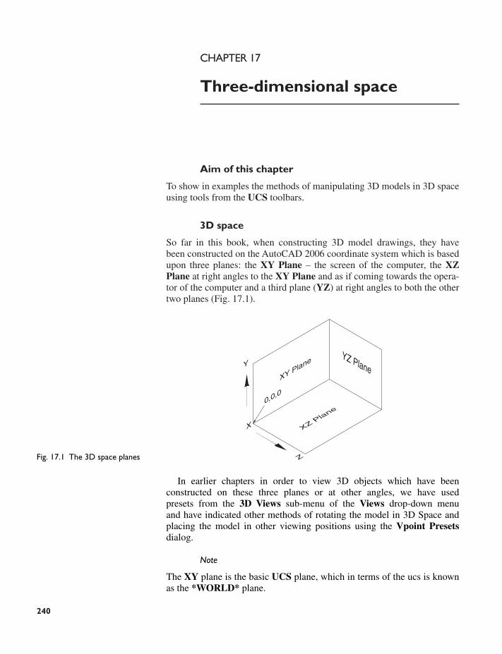
240
CHAPTER 17
Three-dimensional space
Aim of this chapter
To show in examples the methods of manipulating 3D models in 3D spaceusing tools from the UCS toolbars.
3D space
So far in this book, when constructing 3D model drawings, they havebeen constructed on the AutoCAD 2006 coordinate system which is basedupon three planes: the XY Plane – the screen of the computer, the XZPlane at right angles to the XY Plane and as if coming towards the opera-tor of the computer and a third plane (YZ) at right angles to both the othertwo planes (Fig. 17.1).
XY Plane
X
Y
0,0,0
XZ Pla
ne
Z
YZ Plane
Fig. 17.1 The 3D space planes
In earlier chapters in order to view 3D objects which have beenconstructed on these three planes or at other angles, we have usedpresets from the 3D Views sub-menu of the Views drop-down menuand have indicated other methods of rotating the model in 3D Space andplacing the model in other viewing positions using the Vpoint Presetsdialog.
Note
The XY plane is the basic UCS plane, which in terms of the ucs is knownas the *WORLD* plane.

Three-dimensional space 241
The User Coordinate System (UCS)
The UCS allows the operator to place the AutoCAD coordinate systemin any position in 3D space using a variety of UCS tools (commands).Features of the UCS can be called either by entering ucs at the commandline, or by selection from the Tools drop-down menu (Fig. 17.2), or fromthe two UCS toolbars – UCS and UCS II (Fig. 17.3).
Fig. 17.2 The two sub-menusfrom the Tools drop-down menu
Fig. 17.3 The tools from the twoUCS toolbars

242 Introduction to AutoCAD 2006
If ucs is entered at the command line, it shows:
Command: enter ucs right-clickCurrent ucs name: *WORLD*Enter an option [New/Move/orthoGraphic/Prev/Restore/Save/Del/
Apply/?/World] �World�: enter n (New) right-clickSpecify origin of UCS or [ZAxis/3point/OBject/Face/View/X/Y/Z]
�0,0,0�:
And from these prompt lines a selection can be made.The two sub-menus – Orthographic UCS and New UCS – from the
Tools drop-down menu provide a similar set of tools.The tools may also be called from the UCS or UCS II toolbars.
The variable UCSFOLLOW
For the UCS to operate, the variable UCSFOLLOW must first be set onas follows:
Command: enter ucsfollow right-clickEnter new value for UCSFOLLOW �0�: enter 1 right-clickCommand:
The UCS icon
The UCS icon which indicates the direction of the three coordinate axesX, Y and Z is by default shown at the bottom left-hand corner of theAutoCAD drawing area as arrows pointing in the directions of the axes.When working in 2D, only the X and Y axes are shown, but when thedrawing area is in a 3D view all three coordinate arrows are shown,except when the model is in the XY plane. The icon can be turned offas follows:
Command: enter ucsicon right-clickEnter an option [ON/OFF/Noorigin/ORigin/Properties] �ON�:
To turn the icon off, enter off in response to the prompt line and the icondisappears from the screen.
The appearance of the icon can be changed by entering p (Properties)in response to the prompt line. The UCS Icon dialog appears in whichchanges can be made to the shape, line width and colour of the iconif wished.
Types of UCS icon
The shape of the icon can be varied partly when changes are made in theUCS Icon dialog but also according to whether the AutoCAD drawingarea is in 2D, 3D or Paper Space. A different form of 3D icon will appearwhen using the 3D Orbit tool (Fig. 17.4).

Three-dimensional space 243
Examples of changing planes using the UCS
First example – changing UCS planes (Fig. 17.6)
1. Set UCSFOLLOW to 1 (ON).2. Place the screen in 3D Views/Front and Zoom to 1.3. Construct the pline outline in Fig. 17.5 and extrude to a height
of 120.
Fig. 17.4 Types of UCS icon
15
160120°
150
15Fig. 17.5 First example –Changing UCS planes – plinefor extrusion
Fig. 17.6 First example –Changing UCS planes
4. Place in the SW Isometric view and Zoom to 1.5. With the Fillet tool, fillet corners to a radius of 20.6. At the command line:
Command: enter ucs right-clickCurrent ucs name: *WORLD*Enter an option [New/Move/orthoGraphic/Prev/Restore/Save/Del/
Apply/?/World] �World�: enter n (New) right-clickSpecify origin of new UCS or [ZAxis/3point/OBject/Face/
View/X/Y/Z/]: enter f (Face) right-click

244 Introduction to AutoCAD 2006
Select face of solid object: pick the sloping face – its outline high-lights
Enter an option [Next/Xflip/Yflip] �accept�: right-clickCommand:
And the 3D model changes its plane so that the sloping face is nowon the new UCS plane. Zoom to 1.
7. On this new UCS, construct four cylinders of radius 7.5 and height �15(note the minus) and subtract them from the face.
8. Enter ucs at the command line again and right-click to place themodel in the *WORLD* UCS – that being the plane in which theconstruction commenced.
9. Place four cylinders of the same radius and height into position in thebase of the model and subtract them from the model.
10. Place the 3D model in the SW Isometric view and call Hide.
Second example – UCS (Fig. 17.9)
The 3D model for this example is a steam venting valve from a machineof which a two-view third angle projection is shown (Fig. 17.7).
SQ
80
SQ
120
R2020
1010
Hole Ø30
R10
Bolts M10
R5
60 40
Holes Ø1010
35
Hole Ø70
9025
Fig. 17.7 Second example UCS –the orthographic projection of asteam venting valve
1. Make sure that UCSFOLLOW is set to 1.2. The UCS plane is the *WORLD* plane. Construct the 120 square
plate at the base of the central portion of the valve. Construct fivecylinders for the holes in the plate. Subtract the five cylinders fromthe base plate.
3. Construct the central part of the valve – a filleted 80 square extrusionwith a central hole.

Three-dimensional space 245
4. Place the models in the UCS orthoGonal/Front plane.5. With the Move tool, move the central portion vertically up by 10.6. With the Copy tool, copy the base up to the top of the central
portion.7. With the Union tool form a single 3D model of the three parts.8. Make the layer Construction current.9. Place the model in the UCS *WORLD* plane. Construct the sep-
arate top part of the valve – a plate forming a union with a hexagonalplate and with holes matching those of the other parts.
10. Place the scene so far in the UCS orthoGonal/Front plane and movethe parts of the top into their correct positions relative to each otherand with Union and Subtract tools, complete the part. This will bemade easier if the layer 0 is turned off.
11. Turn layer 0 on and move the top into its correct position relative tothe main part of the valve. Then with the Mirror tool, mirror the topto produce the bottom of the assembly (Fig. 17.8).
12. While in the *FRONT* UCS construct the three parts of a 3D modelof the extrusion to the main body.
13. In the UCS *WORLD* move the parts into their correct positionsrelative to each other and with Union form a union of the two filletedrectangular extrusions and the main body. Then with Subtract, sub-tract the cylinder from the whole (Fig. 17.9).
14. In the UCS *FRONT* plane, construct one of the bolts as shown inFig. 17.10, forming a solid of revolution from a pline. Then add ahead to the bolt and with Union add it to the screw.
15. With the Copy tool, copy the bolt 7 times to give 8 bolts. WithMove, and working in the UCS *WORLD* and *FRONT*planes, move the bolts into their correct positions relative to the 3Dmodel.
16. Save the model to a suitable file name.17. Finally move all the parts away from each other to form an exploded
view of the assembly (Fig. 17.11).
Third example – UCS (Fig. 17.15)
1. Set UCSFOLLOW to 1.2. Place the drawing area in the UCS *FRONT* view.3. Construct the outline in Fig. 17.12 and extrude to a height of 120.4. Either click the 3 Point UCS tool icon in the UCS toolbar
(Fig. 17.13) or at the command line (Fig. 17.14 shows the three UCSpoints):
Command: enter ucs right-clickCurrent ucs name: *RIGHT*Enter an option [prompts]: enter n (New) right-clickSpecify origin of UCS or [prompts]: enter 3 (3point) right-clickSpecify new origin point: pickSpecify point on positive portion of X-axis: pick
5
20
Fig. 17.8 Second exampleUCS – construction up to item11 � rendering
Fig. 17.9 Second exampleUCS – items 12 and 13 � rendering
Fig. 17.10 Second example UCS –pline for the bolt
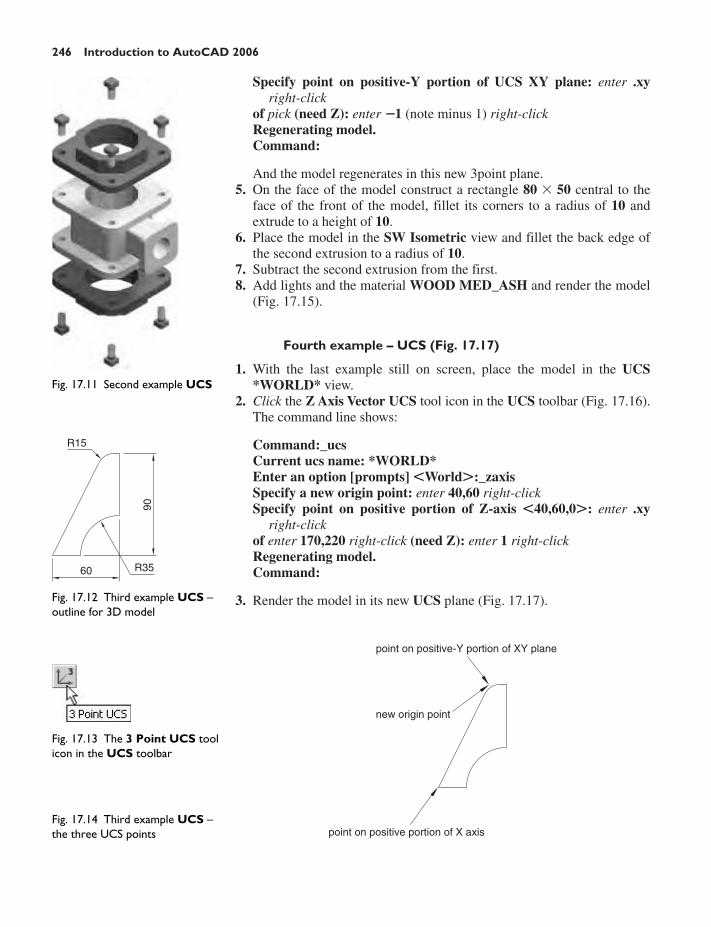
246 Introduction to AutoCAD 2006
Specify point on positive-Y portion of UCS XY plane: enter .xyright-click
of pick (need Z): enter �1 (note minus 1) right-clickRegenerating model.Command:
And the model regenerates in this new 3point plane.5. On the face of the model construct a rectangle 80 � 50 central to the
face of the front of the model, fillet its corners to a radius of 10 andextrude to a height of 10.
6. Place the model in the SW Isometric view and fillet the back edge ofthe second extrusion to a radius of 10.
7. Subtract the second extrusion from the first.8. Add lights and the material WOOD MED_ASH and render the model
(Fig. 17.15).
Fourth example – UCS (Fig. 17.17)
1. With the last example still on screen, place the model in the UCS*WORLD* view.
2. Click the Z Axis Vector UCS tool icon in the UCS toolbar (Fig. 17.16).The command line shows:
Command:_ucsCurrent ucs name: *WORLD*Enter an option [prompts] �World�:_zaxisSpecify a new origin point: enter 40,60 right-clickSpecify point on positive portion of Z-axis �40,60,0�: enter .xy
right-clickof enter 170,220 right-click (need Z): enter 1 right-clickRegenerating model.Command:
3. Render the model in its new UCS plane (Fig. 17.17).
Fig. 17.11 Second example UCS
R15
90
R3560
point on positive-Y portion of XY plane
point on positive portion of X axis
new origin point
Fig. 17.12 Third example UCS –outline for 3D model
Fig. 17.13 The 3 Point UCS toolicon in the UCS toolbar
Fig. 17.14 Third example UCS –the three UCS points

Three-dimensional space 247
Saving UCS views
If a number of different UCS planes are used in connection with the con-struction of a 3D model, each can be saved to a different name andrecalled when required. To save the UCS plane in which a 3D modeldrawing is being constructed, either click the UCS tool icon in the UCStoolbar (Fig. 17.18) or enter ucs at the command line:
Command:_ucsCurrent ucs name: NW IsometricEnter an option [prompts]: enter s (Save) right-clickEnter name to save current UCS: enter SW Isometric right-clickRegenerating model.Command:
Fig. 17.15 Third example UCS
Fig. 17.16 The Z Axis VectorUCS icon in the UCS toolbar
Fig. 17.17 Fourth example UCS
Fig. 17.18 The UCS icon in theUCS toolbar
Fig. 17.19 The Display UCSDialog icon in the UCS II toolbar
Now click the Display UCS Dialog tool icon in the UCS II toolbar andthe UCS dialog appears (Figs 17.19 and 17.20) showing the names of theviews saved in the current drawing.
Constructing 2D objects in 3D space
In previous pages of this book there have been examples of 2D objectsconstructed with the Polyline, Line, Circle and other 2D tools to form theoutlines for extrusions and solids of revolution. These outlines have beendrawn on planes set either from the 3D Views sub-menu of the Viewdrop-down menu, or in UCS planes such as the UCS *RIGHT*,*FRONT* and *LEFT* planes.

248 Introduction to AutoCAD 2006
First example – 2D outlines in 3D space (Fig. 17.23)
1. Construct a 3point UCS to the following points:
origin point: 80,90X-axis point: 290,150positive-Y point: .xy of 80,90(need Z): enter 1.
2. On this 3point UCS construct a 2D drawing of the plate to the dimen-sions given in Fig. 17.21, using the Polyline, Ellipse and Circle tools.
Fig. 17.20 The UCS dialog
Holes Ø20
60 140
30
3090
190
40
All chamfers are 10 × 10
Fig. 17.21 First example – 2Doutlines in 3D space
3. Save the UCS plane in the UCS dialog to the name 3point.4. Place the drawing area in the SW Isometric view (Fig. 17.22).5. With the Region tool form regions of the six parts of the drawing and with
the Subtract tool, subtract the circles and ellipse from the main outline.6. Extrude the region to a height of 10 (Fig. 17.23).
Fig. 17.22 First example – 2Doutlines in 3D space. Theoutline in a SW Isometric view
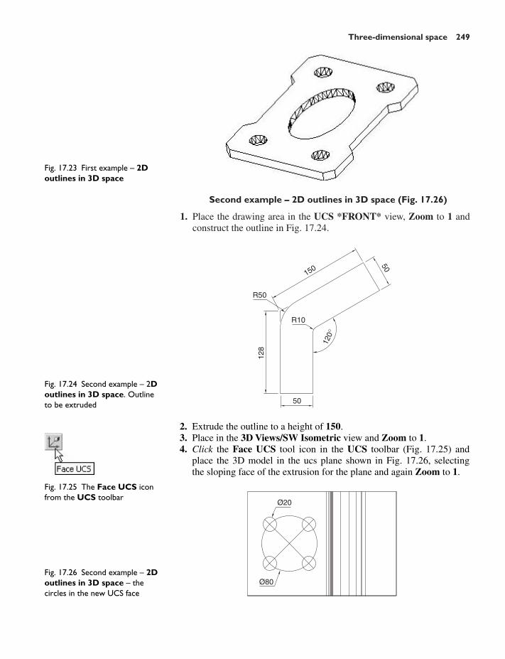
Three-dimensional space 249
Second example – 2D outlines in 3D space (Fig. 17.26)
1. Place the drawing area in the UCS *FRONT* view, Zoom to 1 andconstruct the outline in Fig. 17.24.
Fig. 17.23 First example – 2Doutlines in 3D space
50
50
128
120°
R10
R50
150
Ø20
Ø80
Fig. 17.24 Second example – 2Doutlines in 3D space. Outlineto be extruded
Fig. 17.25 The Face UCS iconfrom the UCS toolbar
Fig. 17.26 Second example – 2Doutlines in 3D space – thecircles in the new UCS face
2. Extrude the outline to a height of 150.3. Place in the 3D Views/SW Isometric view and Zoom to 1.4. Click the Face UCS tool icon in the UCS toolbar (Fig. 17.25) and
place the 3D model in the ucs plane shown in Fig. 17.26, selectingthe sloping face of the extrusion for the plane and again Zoom to 1.

250 Introduction to AutoCAD 2006
5. With the Circle tool draw five circles as shown in Fig. 17.26.6. Form a region from the five circles and with Union form a union of
the regions.7. Extrude the region to a height of �60 (Note the minus) – higher than
the width of the sloping part of the 3D model.8. Place the model in the SW Isometric view and subtract the extruded
region from the model.9. With the Fillet tool, fillet the upper corners of the slope of the main
extrusion to a radius of 30.10. Place the model in another UCS FACE plane and construct a filleted
pline of sides 80 and 50 and filleted to a radius of 20. Extrude to aheight of �60 and subtract the extrusion from the 3D model.
11. Place in the SW Isometric view and render (Fig. 17.27).
Revision notes
1. The UCS (User Coordinate System) tools can be called from the twotoolbars UCS and UCS II or from sub-menus from the Tools drop-downmenu.
2. The variable UCSFOLLOW must first be set on (to 1) before operationsof the UCS can be brought into action.
3. There are several types of UCS icons – 2D (different types), 3D (differenttypes), 3D Orbit, Pspace.
4. The position of the plane in 3D space on which a drawing is beingconstructed can be varied using tools from the UCS.
5. The different planes on which drawings are constructed in 3D spacecan be saved in the UCS dialog.
Exercises
1. The two-view projection shows an angle bracket in which two pins areplaced in holes in each of the arms of the bracket as shown in Fig. 17.29.Construct a 3D model of the bracket and its pins. Add lighting to thescene and materials to the parts of the model and render (Fig. 17.28).
2. The two-view projection (Fig. 17.31) shows a stand consisting of twohexagonal prisms. Circular holes have been cut right through each faceof the smaller hexagonal prism and rectangular holes with roundedends have been cut right through the faces of the larger.
Construct a 3D model of the stand. When completed add suitable light-ing to the scene. Then add a material to the model and render (Fig. 17.30).
3. The two-view projection (Fig. 17.32) shows a ducting pipe. Constructa 3D model drawing of the pipe. Place in a SW Isometric view, addlighting to the scene and a material to the model and render.
4. A point marking device is shown in the two-view projection in Fig. 17.33.The device is composed of three parts – a base, an arm and a pin.
Construct a 3D model of the assembled device and add appropriatematerials to each part. Then add lighting to the scene and render in aSW Isometric view (Fig. 17.34).
Fig. 17.27 Second example – 2Doutlines in 3D space
Fig. 17.28 Exercise 1 – a rendering
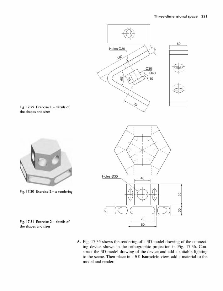
Three-dimensional space 251
Holes Ø30
60
Ø30Ø40
10
75
60° 30
180
15
Fig. 17.29 Exercise 1 – details ofthe shapes and sizes
Holes Ø30 4660
30
70
80
20
Fig. 17.30 Exercise 2 – a rendering
Fig. 17.31 Exercise 2 – details ofthe shapes and sizes
5. Fig. 17.35 shows the rendering of a 3D model drawing of the connect-ing device shown in the orthographic projection in Fig. 17.36. Con-struct the 3D model drawing of the device and add a suitable lightingto the scene. Then place in a SE Isometric view, add a material to themodel and render.

252 Introduction to AutoCAD 2006
R45
R40
R15
R145
R105
R65
Holes Ø10
Hol
e Ø
7012
0
Ø10
65
20 3 35
20
45
490R45
Hole Ø50
R10 15
Holes Ø20
R20
R15
R32
R20
R45
15010
50
20 90
180
Fig. 17.32 Exercise 3 – details ofthe shapes and sizes
Fig. 17.33 Exercise 4 – details ofthe shapes and sizes
Fig. 17.34 Exercise 4 – a rendering
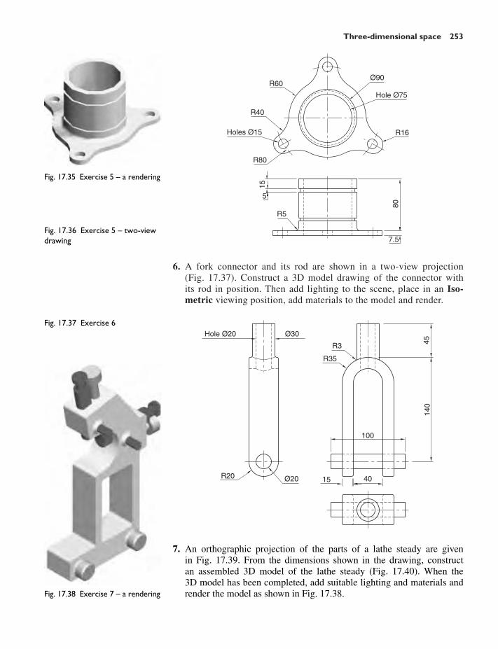
Three-dimensional space 253
6. A fork connector and its rod are shown in a two-view projection(Fig. 17.37). Construct a 3D model drawing of the connector withits rod in position. Then add lighting to the scene, place in an Iso-metric viewing position, add materials to the model and render.
Fig. 17.35 Exercise 5 – a rendering
Ø90
Hole Ø75
R16
80
7.5
R5
5
15
R80
Holes Ø15
R40
R60
Fig. 17.36 Exercise 5 – two-viewdrawing
Hole Ø20 Ø30
R3
R35
10014
045
4015Ø20R20
Fig. 17.37 Exercise 6
Fig. 17.38 Exercise 7 – a rendering
7. An orthographic projection of the parts of a lathe steady are givenin Fig. 17.39. From the dimensions shown in the drawing, constructan assembled 3D model of the lathe steady (Fig. 17.40). When the3D model has been completed, add suitable lighting and materials andrender the model as shown in Fig. 17.38.

254 Introduction to AutoCAD 2006
Dimensions in millimeters
A5
16
123
M8
A
Name:A. Student
Scale:1:1
Date: Title:15/03/2006 LATHE STEADY
1
DO NOT SCALE THIS DRAWING
6
326
45
90°
30
80° R24
13
10
63HOLES ∅10∅20
98 13
40 10
M10 ∅20
M10 ∅20
∅1612
10
40
45 10
580 2
3
BOSS ∅16TAPPED M8
30
4
30 × ∅10
2 3
5
6
2
31
4Fig. 17.40 Exercise 7 – anisometric drawing
Fig. 17.39 Exercise 7 – details

255
CHAPTER 18
3D Surface models
Aims of this chapter
1. To introduce the idea of 3D surfaces.2. To compare 3D surface models with 3D solid drawing models.3. To give examples of 3D surface models.
3D surface meshes
3D surface models will be introduced in this chapter. The 3D modelsdescribed in earlier chapters have all be constructed using the tools fromthe Solids toolbar. 3D surface models are constructed using tools from theSurfaces toolbar (see page 174). 3D surface model drawings areconstructed from 3D surface meshes. In some instances it appears as if3D solid models are the same as 3D surface models, but in fact there aredistinct differences.
1. The surface meshes of 3D solid models are controlled by the settingsof the variable ISOLINES.
2. The surface meshes of 3D surface models are controlled either by thenumber of segments or by the two variables SURFTAB1 and/orSURFTAB2.
3. The Boolean operators Union, Subtract and Intersect can be used tojoin, subtract or intersect 3D model objects, but have no action whenused with 3D surface objects.
Comparisons between Solids and Surfaces tools
First example – comparing 3D solid and 3D surface models(Fig. 18.3)
The three 3D cubes shown in the upper drawing of Fig. 18.3 have beenconstructed as follows:
Left-hand cube: using the Line tool.Central cube: using the Box tool from the Solids toolbar (Fig. 18.1).Right-hand cube: using the Box tool from the Surfaces toolbar (Fig. 18.2).
The lower three drawings of Fig. 18.3 show the results of calling theHide tool on each of the three upper drawings.
Fig. 18.1 The Box tool icon fromthe Solids toolbar

256 Introduction to AutoCAD 2006
Second example – Surfaces tool – Cone (Fig. 18.5)
The three cylinders were all constructed using the Cone tool from theSurfaces toolbar (Fig. 18.4).
Fig. 18.2 The Box tool icon fromthe Surfaces toolbar
Line cube Solid box cubeBefore Hide
Surfaces box
After Hide
Fig. 18.3 First example –comparing 3D solid and 3Dsurface models
Fig. 18.4 The Cone tool iconfrom the Surfaces toolbar
Fig. 18.5 Second example –Surfaces tool – Cone
When using the Cone tool, the last prompt line is:
Enter number of segments for surface of cone: enter a figure right-click
The upper three cones (top and bottom of cone are of sameradius) show the number of segments entered in response to thisprompt line.
Note that when Hide is called, the upper surface of the cylinders donot have surface meshes and so are open.

3D Surface models 257
Third example – Solids tool – Cylinder (Fig. 18.7)
The upper three cylinders in this example were constructed using theCylinder tool from the Solids toolbar (Fig. 18.6).
Fig. 18.6 The Cylinder tool iconfrom the Solids toolbar
Fig. 18.7 Third example – Solidstool – Cylinder
Fig. 18.8 Fourth example –Surfaces tool – Edgesurf
The lower three drawings show the results of calling Hide to the threecylinders in the upper drawings.
Note that the upper surface of the three cylinders hide the rest of thelines behind the top and that all three cylinders assume the same meshappearance when Hide is called.
Fourth example – Surfaces tool – Edgesurf (Fig. 18.8)
When constructing 3D surface models using tools such as the EdgeSurface tool from the Surfaces toolbar, both the Surftab1 and theSurftab2 variables may need resetting.
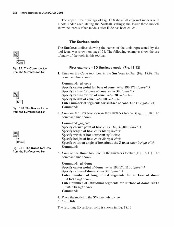
258 Introduction to AutoCAD 2006
The upper three drawings of Fig. 18.8 show 3D edgesurf models witha note under each stating the Surftab settings; the lower three modelsshow the three surface models after Hide has been called.
The Surface tools
The Surfaces toolbar showing the names of the tools represented by thetool icons was shown on page 174. The following examples show the useof many of the tools in this toolbar.
First example – 3D Surfaces model (Fig. 18.12)
1. Click on the Cone tool icon in the Surfaces toolbar (Fig. 18.9). Thecommand line shows:
Command:_ai_coneSpecify center point for base of cone: enter 190,170 right-clickSpecify radius for base of cone: enter 30 right-clickSpecify radius for top of cone: enter 30 right-clickSpecify height of cone: enter 80 right-clickEnter number of segments for surface of cone �16�: right-clickCommand:
2. Click on the Box tool icon in the Surfaces toolbar (Fig. 18.10). Thecommand line shows:
Command:_ai_boxSpecify corner point of box: enter 160,140,80 right-clickSpecify length of box: enter 60 right-clickSpecify width of box: enter 60 right-clickSpecify height of box: enter 30 right-clickSpecify rotation angle of box about the Z axis: enter 0 right-clickCommand:
3. Click on the Dome tool icon in the Surfaces toolbar (Fig. 18.11). Thecommand line shows:
Command:_ai_domeSpecify center point of dome: enter 190,170,110 right-clickSpecify radius of dome: enter 30 right-clickEnter number of longitudinal segments for surface of dome
�16�: right-clickEnter number of latitudinal segments for surface of dome �8�:
enter 16 right-clickCommand:
4. Place the model in the SW Isometric view.5. Call Hide.
The resulting 3D surfaces solid is shown in Fig. 18.12.
Fig. 18.9 The Cone tool iconfrom the Surfaces toolbar
Fig. 18.11 The Dome tool iconfrom the Surfaces toolbar
Fig. 18.10 The Box tool iconfrom the Surfaces toolbar

3D Surface models 259
Note
Try forming a union of the three 3D surface objects by clicking the Uniontool from the Solids Editing toolbar. The command line will show:
Command:_unionSelect objects: pick the cylinder 1 foundSelect objects: pick the box 1 found, 2 totalSelect objects: pick the dome 1 found, 3 totalSelect objects: right-clickAt least 2 solids or coplanar regions must be selected.Command:
It will be seen that the three surface models will not form a union. Test bymoving any one of the three surface models.
Second example – Surfaces model (Fig. 18.14)
1. Construct the same cylinder (using the Cone tool from Surfaces) asfor the first example.
2. Click on the Torus tool in the Surfaces toolbar (Fig. 18.13). Thecommand line shows:
Command:_ai_torusSpecify center point of torus: enter 190,170,25 right-clickSpecify radius of torus: enter 35 right-clickSpecify radius of tube: enter 5 right-clickEnter number of segments around the tube circumference �16�:
right-clickEnter number of segments around torus circumference �16�:
right-clickCommand:
3. Construct a similar torus at a height of 55 above the XY plane.4. Add a Dome of radius 30 at a height above the XY plane of 80.5. Place the model in the SW Isometric view. Zoom to 1.6. Call Hide.
Third example – Surfaces model (Fig. 18.17)
1. Construct the plines as shown in Fig. 18.15.2. Set SURFTAB1 to 24.3. Set SURFTAB2 to 6.4. Click the Revolved Surface tool icon in the Surfaces toolbar (Fig. 18.16).
The command line shows:
Command:_revsurfCurrent wire frame density: SURFTAB1�24 SURFTAB2�6Select object to revolve: pick the curved plineSelect object that defines the axis of revolution: pickSpecify start angle �0�: right-clickSpecify included angle �360�: right-clickCommand:
Fig. 18.14 Second example –Surfaces model
Fig. 18.13 The Torus tool iconfrom the Surfaces toolbar
Fig. 18.12 First example – 3DSurfaces model

260 Introduction to AutoCAD 2006
5. Erase the axis of revolution pline.6. Place in a SW Isometric view, Zoom to 1 and call Hide.
Fourth example – Surfaces model (Fig. 18.19)
1. Set Surftab1 to 2.2. In the UCS *WORLD* construct a hexagon of edge length 35.3. In the UCS *FRONT* and in the centre of the hexagon construct a
pline of height 100.4. Place the drawing area in the SW Isometric view.5. Click on the Tabulated Surface tool in the Surfaces toolbar (Fig. 18.18).
The command line shows:
Command:_tabsurfCurrent wire frame density: SURFTAB1�6Select objects for path curve: pick the hexagonSelect object for direction vector: pick the plineCommand:
6. Call Hide.
Fifth example – Surfaces model (Fig. 18.22)
1. In the UCS *FRONT* construct the pline as shown in Fig. 18.20.2. In the UCS *WORLD*, Zoom to 1 and copy the pline to a vertical
distance of 120.
110 20 R15
315Axis of revolution
R25
R30
0Fig. 18.15 Third example –Surfaces model – pline outline
Fig. 18.16 The RevolvedSurface tool icon from theSurfaces toolbar
Fig. 18.17 Third example –Surfaces model
Fig. 18.18 The TabulatedSurface tool icon from theSurfaces toolbar
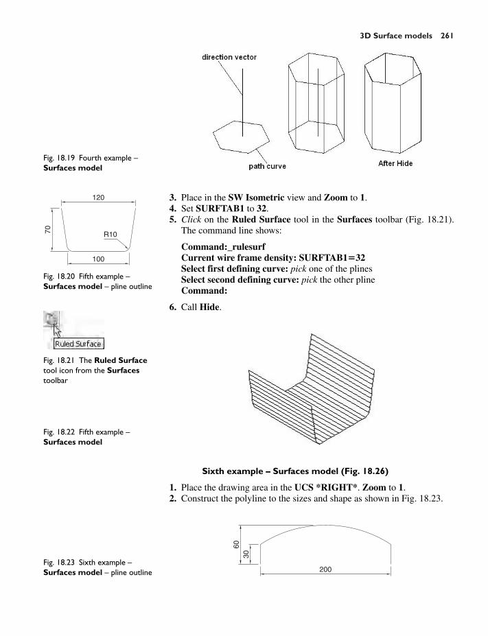
3D Surface models 261
120
70 R10
100
Fig. 18.20 Fifth example –Surfaces model – pline outline
Fig. 18.19 Fourth example –Surfaces model
Fig. 18.21 The Ruled Surfacetool icon from the Surfacestoolbar
Fig. 18.22 Fifth example –Surfaces model
3. Place in the SW Isometric view and Zoom to 1.4. Set SURFTAB1 to 32.5. Click on the Ruled Surface tool in the Surfaces toolbar (Fig. 18.21).
The command line shows:
Command:_rulesurfCurrent wire frame density: SURFTAB1�32Select first defining curve: pick one of the plinesSelect second defining curve: pick the other plineCommand:
6. Call Hide.
Sixth example – Surfaces model (Fig. 18.26)
1. Place the drawing area in the UCS *RIGHT*. Zoom to 1.2. Construct the polyline to the sizes and shape as shown in Fig. 18.23.
200
3060
Fig. 18.23 Sixth example –Surfaces model – pline outline

262 Introduction to AutoCAD 2006
3. Place the drawing area in the UCS *WORLD*. Zoom to 1.4. Copy the pline to the right by 250.5. Place the drawing in the SW Isometric view and Zoom to 1.6. With the Line tool, draw lines between the ends of the two plines
using the endpoint osnap (Fig. 18.24). Note that if polylines are drawnthey will not be accurate at this stage.
7. Set SURFTAB1 to 32 and SURFTAB2 to 64.8. Click on the Edge Surface tool icon in the Surfaces toolbar (Fig. 18.25).
The command line shows:
Command:_edgesurfCurrent wire frame density: SURFTAB1�32 SURFTAB2�64Select object 1 for surface edge: pick one of the lines (or plines)Select object 1 for surface edge: pick the next adjacent line (or pline)Select object 1 for surface edge: pick the next adjacent line (or pline)Select object 1 for surface edge: pick the last line (or pline)Command:
9. Call Hide.
The result is shown in Fig. 18.26.
Fig. 18.24 Sixth example –Surfaces model – adding linesjoining the outlines
Fig. 18.25 The Edge Surfacetool icon from the Surfacestoolbar
Fig. 18.26 Sixth example –Surfaces model
The action of Pedit on a 3D surface (Fig. 18.27)
Open the drawing file saved for the last 3D drawing model (the edgesurfmodel) and copy it twice. Then call the Polyline Edit tool. The commandline shows:
Command:_peditSelect polyline or [Multiple]: pick the first copyEnter an option [Edit vertex/Smooth surface/Desmooth/Mclose/
Nclose/Undo]: enter s (Smooth surface) right-clickEnter an option [Edit vertex/Smooth surface/Desmooth/Mopen/
Nclose/Undo]: right-clickCommand:
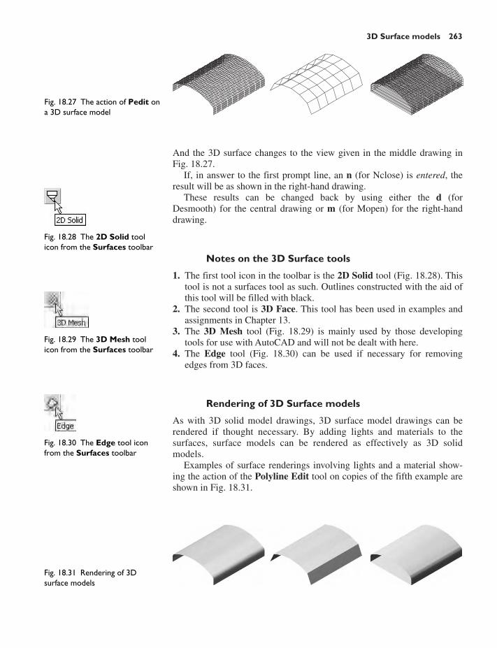
3D Surface models 263
And the 3D surface changes to the view given in the middle drawing inFig. 18.27.
If, in answer to the first prompt line, an n (for Nclose) is entered, theresult will be as shown in the right-hand drawing.
These results can be changed back by using either the d (forDesmooth) for the central drawing or m (for Mopen) for the right-handdrawing.
Notes on the 3D Surface tools
1. The first tool icon in the toolbar is the 2D Solid tool (Fig. 18.28). Thistool is not a surfaces tool as such. Outlines constructed with the aid ofthis tool will be filled with black.
2. The second tool is 3D Face. This tool has been used in examples andassignments in Chapter 13.
3. The 3D Mesh tool (Fig. 18.29) is mainly used by those developingtools for use with AutoCAD and will not be dealt with here.
4. The Edge tool (Fig. 18.30) can be used if necessary for removingedges from 3D faces.
Rendering of 3D Surface models
As with 3D solid model drawings, 3D surface model drawings can berendered if thought necessary. By adding lights and materials to thesurfaces, surface models can be rendered as effectively as 3D solidmodels.
Examples of surface renderings involving lights and a material show-ing the action of the Polyline Edit tool on copies of the fifth example areshown in Fig. 18.31.
Fig. 18.27 The action of Pedit ona 3D surface model
Fig. 18.30 The Edge tool iconfrom the Surfaces toolbar
Fig. 18.29 The 3D Mesh toolicon from the Surfaces toolbar
Fig. 18.28 The 2D Solid toolicon from the Surfaces toolbar
Fig. 18.31 Rendering of 3Dsurface models

264 Introduction to AutoCAD 2006
Revision notes
1. The density of 3D surface meshes of surface models are controlled bythe two set variables SURFTAB1 and SURFTAB2.
2. The Solids tools Union, Subtract and Intersect (the Boolean operators)cannot be used with surface models.
3. When constructing a surface 3D cylinder, the Cone tool from theSurfaces toolbar must be used.
4. Surfaces formed with the Ruled Surface tool require two outlinesfrom which the surface can be obtained.
5. Surfaces formed with the Edge Surface tool require four edges fromwhich to form the surface. The edges must meet each other at theirends for the surface to form.
6. 3D surface models can be rendered using the same methods as areused when rendering 3D solid models.
Exercises
1. In the UCS *WORLD* construct the polyline outline as shown inFig. 18.32. With the Tabulated Surface tool create a girder of length200 from the outline (left-hand drawing of Fig. 18.33). Using theEdge Surface tool, construct a surface to cover the top end of thegirder. Render the girder after adding suitable lights and the materialCOPPER (right-hand drawing of Fig. 18.33).
9010 5
1085R10
Fig. 18.33 Exercise 1 – theTabulated Surface and therendering
Fig. 18.32 Exercise 1 – the outlinefrom which the surface model isformed
2. Using the Polyline tool construct arcs as shown in Fig. 18.34. Usingthe UCS 3point option construct semicircles joining both ends
255,265
200,265
245,240
180,270
170,220175,220
220,175
220,145
Fig. 18.34 Exercise 2 – the arcson which the exercise is based

3D Surface models 265
of the arcs as shown in Fig. 18.35. With the Edge Surface tooland with the SURFTAB variables set to suitable sizes, construct asurface from the four arcs (Fig. 18.36). Using the Mirror tool,mirror the surface twice to obtain the hook shape as shown in therendering in Fig. 18.37. Render the hook after adding lighting andthe material BRASS GIFMAP.
3. Construct a surface of revolution from the polyline outline given inthe left-hand drawing of Fig. 18.38. Add lighting and the materialBLUE GLASS and after placing the surface model in a suitableisometric viewing position render the model – right-hand illustration(Fig. 18.38).
Fig. 18.37 Exercise 2
Fig. 18.36 Exercise 2 – a surface
Fig. 18.35 Exercise 2 – semi-circles at end of arcs
R12.5
145
60
5
560
3020
R10 R45
R60
Fig. 18.38 Exercise 3

266 Introduction to AutoCAD 2006
Fig. 18.40 Exercise 4
60 40 6060 30 80
130
10
90
10
180Fig. 18.41 Exercise 5 – sizes ofthe parts of the model
Fig. 18.42 Exercise 5
17090
100
130
Fig. 18.39 Exercise 4 – the twosemi-ellipses
4. In the UCS *WORLD* plane construct two semi-ellipses to the sizesas given in Fig. 18.39. Place in the UCS *FRONT* plane and movethe smaller semi-ellipse vertically upwards by 200 units. Using theRuled Surface tool, form a surface between the two semi-ellipses.Add suitable lighting and a suitable material and render the surface(Fig. 18.40).
5. Using the Pyramid and Box tools from the Surfaces toolbar, constructthe 3D model in Fig. 18.41. Then place the model in the SW Isomet-ric view and using the Hidden shading from the 3D Orbit right-clickmenu, hide lines behind the front faces (Fig. 18.42).

3D Surface models 267
Fig. 18.44 Exercise 6
Sphere ∅80
230
∅20
Cone ∅40
310∅40
135
Fig. 18.43 Exercise 6 – front view
6. Working to the sizes given in the front view in Fig. 18.43, construct the3D surface model shown in the rendering in Fig. 18.44.

268
CHAPTER 19
Editing 3D solid models: More3D models
Aims of this chapter
1. To introduce the use of tools from the Solids Editing toolbar.2. To give examples of the use of the tools from the Solids Editing toolbar.3. To show examples of a variety of 3D solid and 3D surface models.
The Solids Editing tools
The tools from the Solids Editing toolbar have already been illustrated onpage 174. Examples of the results of using some of the tools from thistoolbar are shown in this chapter. These tools are of value if the design of a3D solid model requires to be changed (edited), although some have a valuein constructing solids which cannot easily be constructed using other tools.The Solids Editing tools have no effect when used on 3D surface models.
First example – Extrude Faces tool (Fig. 19.3)
1. Set ISOLINES to 24.2. In the UCS *RIGHT* plane construct a cylinder of radius 30 and
height 30 (Fig. 19.1).
R40
40
40 45 70Fig. 19.1 First example –Extrude Faces tool – first stages
3. In the UCS *FRONT* view construct the pline in Fig. 19.1. Mirrorthe pline to the other end of the cylinder.
4. In the UCS *WORLD* move the pline to lie central to the cylinder.5. Place the screen in the SW Isometric view.6. Click the Extrude Faces tool icon in the Solids Editing toolbar
(Fig.19.2). The command line shows:
Command:_solideditEnter a solids editing option [Face/Edge/Body/Undo/eXit]:_face
Fig. 19.2 The Extrude Facestool icon from the SolidsEditing toolbar

Editing 3D solid models 269
Enter a face editing option [Extrude/Move/Rotate/Offset/Taper/Delete/Copy/coLor/Undo/eXit]:_extrude
Select faces or [Undo/Remove/ALL]: pick the left-hand face of thecylinder 2 faces found
Select faces or [Undo/Remove/ALL]: pick highlighted faces whichare not to be extruded 1 found. 1 removed
Select faces or [Undo/Remove/ALL]: right-clickSpecify height of extrusion or [Path]: enter p right-clickSelect extrusion path: pick the plineSolids editing automatic checking. SOLIDCHECK�0
7. Repeat the operation using the plane at the other end of the cylinder.8. Render the resulting edited 3D model (Fig. 19.3).
Notes
1. Note the prompt line which includes the statement SOLIDCHECK�0.If the variable SOLIDCHECK is set on (to 1) the prompt lines change toinclude the lines SOLIDCHECK�1, Solid validation started andSolid validation completed.
2. When a face is picked other faces become highlighted, using theRemove option of the prompt line Select faces or [Undo/Remove/ALL] allows faces which are not to be extruded to be removed fromthe operation of the tool.
Second example – Extrude Faces tool
1. Construct a hexagonal extrusion just 1 unit high in the UCS*WORLD* plane.
2. Change to the UCS *FRONT* plane and construct the curved pline inFig. 19.4.
3. Back in the UCS *WORLD* move the pline to lie central to the extru-sion.
4. Place in the SW Isometric view and extrude the top face of the extrusionalong the path of the curved pline.
5. Add lighting and a material to the model and render (Fig. 19.5).
Note
This example shows that a face of a 3D solid model can be extrudedalong any suitable path curve. If the polygon on which the extrusionhad been based had been turned into a region, no extrusion could havetaken place. The polygon had to be extruded to give a face to the 3Dsolid.
Third example – Move Faces tool (Fig. 19.7)
1. Construct the 3D solid drawing shown in the left-hand drawing ofFig. 19.7 from three boxes which have been united using the Uniontool.
Fig. 19.3 First example –Extrude Faces tool
Path – a pline
Extruded hexagonof height 1 unit
Fig. 19.4 Second example –Extrude Faces tool – plinefor path

270 Introduction to AutoCAD 2006
2. Click on the Move Faces tool in the Solids Editing toolbar (Fig. 19.6).The command line shows:
Command:_solidedit[prompts]:_faceEnter a face editing option[prompts]:_moveSelect faces of [Undo/Remove/ALL]: pick the face to be moved 2
faces foundSelect faces of [Undo/Remove/ALL]: enter r (remove) right-clickSelect faces of [Undo/Remove/ALL]: pick 2 faces found, 1 removedSelect faces of [Undo/Remove/ALL]: right-clickSpecify a base point or displacement: pickSpecify a second point of displacement: pick[further prompts]:
And the picked face is moved – right-hand drawing of Fig. 19.7.
Fourth example – Offset Faces tool (Fig. 19.8)
1. Construct the 3D solid drawing shown in the left-hand drawing ofFig. 19.8 from a hexagonal extrusion and a cylinder which have beenunited using the Union tool.
2. Click on the Offset Faces tool icon in the Solids Editing toolbar(Fig.19.9). The command line shows:
Command:_solidedit[prompts]:_face[prompts][prompts]:_offsetSelect faces or [Undo/Remove]: pick the bottom face of the 3D model
2 faces foundSelect faces or [Undo/Remove/All]: enter r right-clickSelect faces or [Undo/Remove/All]: pick highlighted faces other than
the bottom face 2 faces found, 1 removedSelect faces or [Undo/Remove/All]: right-clickSpecify the offset distance: enter 30 right-click
3. Repeat, offsetting the upper face of the cylinder by 50 and the right-hand face of the lower extrusion by 15.
Fifth example – Taper Faces tool (Fig. 19.10)
1. Construct the 3D model as in the left-hand drawing of Fig. 19.10.Place in the SW Isometric view.
2. Call Taper Faces. The command line shows:
Command:_solidedit[prompts]:_face[prompts][prompts]:_taper
Fig. 19.7 Third example – MoveFaces tool
Fig. 19.6 The Move Faces toolicon from the Solids Editingtoolbar
Fig. 19.5 Second example –Extrude Faces tool

Editing 3D solid models 271
Select faces or [Undo/Remove]: pick the upper face of the base 2faces found
Select faces or [Undo/Remove/All]: enter r right-clickSelect faces or [Undo/Remove/All]: pick highlighted faces other than
the upper face 2 faces found, 1 removedSelect faces or [Undo/Remove/All]: right-clickSpecify the base point: pick a point on left-hand edge of the faceSpecify another point along the axis of tapering: pick a point on the
right-hand edge of the faceSpecify the taper angle: enter 10 right-click
And the selected face tapers as indicated in the right-hand drawing.
Sixth example – Copy Faces tool (Fig. 19.13)
1. Construct a 3D model to the sizes as given in Fig. 19.12.2. Click on the Copy Faces tool in the Solids Editing toolbar (Fig. 19.11).
The command line shows:
Command:_solidedit[prompts]:_face[prompts]
Fig. 19.8 Fourth example –Offset Faces tool
Fig. 19.9 The Offset Faces toolicon from the Solids Editingtoolbar
Fig. 19.10 Fifth example – TaperFaces tool
Fig. 19.11 The Copy Faces toolicon from the Solids Editingtoolbar
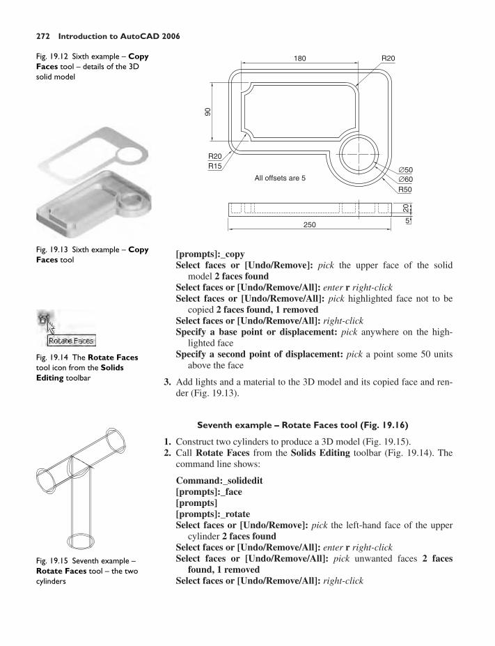
272 Introduction to AutoCAD 2006
[prompts]:_copySelect faces or [Undo/Remove]: pick the upper face of the solid
model 2 faces foundSelect faces or [Undo/Remove/All]: enter r right-clickSelect faces or [Undo/Remove/All]: pick highlighted face not to be
copied 2 faces found, 1 removedSelect faces or [Undo/Remove/All]: right-clickSpecify a base point or displacement: pick anywhere on the high-
lighted faceSpecify a second point of displacement: pick a point some 50 units
above the face
3. Add lights and a material to the 3D model and its copied face and ren-der (Fig. 19.13).
Seventh example – Rotate Faces tool (Fig. 19.16)
1. Construct two cylinders to produce a 3D model (Fig. 19.15).2. Call Rotate Faces from the Solids Editing toolbar (Fig. 19.14). The
command line shows:
Command:_solidedit[prompts]:_face[prompts][prompts]:_rotateSelect faces or [Undo/Remove]: pick the left-hand face of the upper
cylinder 2 faces foundSelect faces or [Undo/Remove/All]: enter r right-clickSelect faces or [Undo/Remove/All]: pick unwanted faces 2 faces
found, 1 removedSelect faces or [Undo/Remove/All]: right-click
180 R20
90
R20R15
All offsets are 5
250 5
20
R50∅60∅50
Fig. 19.12 Sixth example – CopyFaces tool – details of the 3Dsolid model
Fig. 19.13 Sixth example – CopyFaces tool
Fig. 19.14 The Rotate Facestool icon from the SolidsEditing toolbar
Fig. 19.15 Seventh example –Rotate Faces tool – the twocylinders

Editing 3D solid models 273
Specify an axis point or [Axis by object/View/Xaxis/Yaxis/Zaxis]:enter y right-click
Specify the origin of the rotation: pick the upper point of the left-hand face
Specify a rotation angle: enter 10 right-click
3. Add lights and a material, place the 3D model in the SW Isometricview and render. The selected face is rotated as shown in the rendering(Fig. 19.16).
Eighth example – Color Faces tool (Fig. 19.18)
1. Construct a 3D model of a wheel to the sizes as shown in Fig. 19.17.2. Click the Color Faces tool icon in the Solids Editing toolbar. The
command line shows:
Command:_solidedit[prompts]:_face[prompts][prompts]:_colorSelect faces or [Undo/Remove]: pick the inner face of the wheel 2
faces foundSelect faces or [Undo/Remove/All]: enter r right-clickSelect faces or [Undo/Remove/All]: pick highlighted faces other than
the required face 2 faces found, 1 removedEnter new color �ByLayer�: enter 1 (which is red) right-click
3. Add lights and a material to the edited 3D model and render (Fig. 19.18).
Fig. 19.16 Seventh example –Rotate Faces tool
10
5
R550
∅220
∅210
∅200
∅40
R35
R70
R90
Fig. 19.17 Eighth example –Color Faces tool – details of the3D model
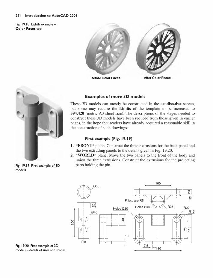
274 Introduction to AutoCAD 2006
Examples of more 3D models
These 3D models can mostly be constructed in the acadiso.dwt screen,but some may require the Limits of the template to be increased to594,420 (metric A3 sheet size). The descriptions of the stages needed toconstruct these 3D models have been reduced from those given in earlierpages, in the hope that readers have already acquired a reasonable skill inthe construction of such drawings.
First example (Fig. 19.19)
1. *FRONT* plane. Construct the three extrusions for the back panel andthe two extruding panels to the details given in Fig. 19.20.
2. *WORLD* plane. Move the two panels to the front of the body andunion the three extrusions. Construct the extrusions for the projectingparts holding the pin.
Fig. 19.18 Eighth example –Color Faces tool
Fig. 19.20 First example of 3Dmodels – details of sizes and shapes
Fig. 19.19 First example of 3Dmodels
Ø50
Ø40Holes Ø20 Holes Ø4020
Fillets are R5
200
Pin
40
10
7.5180
70 110
100
20
5
R20R15
R25
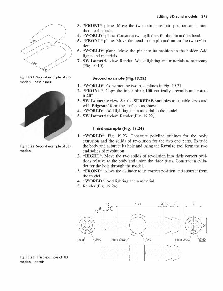
Editing 3D solid models 275
3. *FRONT* plane. Move the two extrusions into position and unionthem to the back.
4. *WORLD* plane. Construct two cylinders for the pin and its head.5. *FRONT* plane. Move the head to the pin and union the two cylin-
ders.6. *WORLD* plane. Move the pin into its position in the holder. Add
lights and materials.7. SW Isometric view. Render. Adjust lighting and materials as necessary
(Fig. 19.19).
Second example (Fig.19.22)
1. *WORLD*. Construct the two base plines in Fig. 19.21.2. *FRONT*. Copy the inner pline 100 vertically upwards and rotate
it 20°.3. SW Isometric view. Set the SURFTAB variables to suitable sizes and
with Edgesurf form the surfaces as shown.4. *WORLD*. Add lighting and a material to the model.5. SW Isometric view. Render (Fig. 19.22).
Third example (Fig. 19.24)
1. *WORLD*. Fig. 19.23. Construct polyline outlines for the bodyextrusion and the solids of revolution for the two end parts. Extrudethe body and subtract its hole and using the Revolve tool form the twoend solids of revolution.
2. *RIGHT*. Move the two solids of revolution into their correct posi-tions relative to the body and union the three parts. Construct a cylin-der for the hole through the model.
3. *FRONT*. Move the cylinder to its correct position and subtract fromthe model.
4. *WORLD*. Add lighting and a material.5. Render (Fig. 19.24).
Fig. 19.22 Second example of 3Dmodels
105 25
10
∅30 ∅40 ∅40Hole ∅60 Hole ∅20R40
160 20 25 25 6060
Fig. 19.23 Third example of 3Dmodels – details
25
100
165
Fig. 19.21 Second example of 3Dmodels – base plines

276 Introduction to AutoCAD 2006
Fig. 19.24 Third example of 3Dmodels
Fig. 19.25 Fourth example of 3Dmodels – the two plines
Fig. 19.26 Fourth example of 3Dmodels – the four plines
R500
300
8570
100160
R20
R20
Fourth example (Fig. 19.27)
1. *RIGHT*. Construct two plines – Fig. 19.25.2. *FRONT*. Move the smaller pline 200 to the right.3. Rotate the two plines to slope at an angle of 10° to the vertical.4. *WORLD*. With the aid of the osnap endpoint construct two pline
arcs joining the bottom ends of the two sloping plines. While in the*WORLD* plane add suitable lighting (Fig. 19.26).
5. SW Isometric. Set the SURFTAB variables to suitable sizes and withEdgesurf from a surface from the four plines.
6. Add a material and render (Fig. 19.27).

Editing 3D solid models 277
R40
R10
R60
60
60 70 90
1020
25
Hole ∅20
80
Fig. 19.29 Fifth example of 3Dmodels
Fig. 19.28 Fifth example of 3Dmodels – details of shapes andsizes
Fifth example (Fig. 19.29)
1. *FRONT*. Construct the three plines needed for the extrusions ofeach part of the model (details Fig. 19.28). Extrude to the givenheights. Subtract the hole from the 20 high extrusion.
Fig. 19.27 Fourth example of 3Dmodels

278 Introduction to AutoCAD 2006
Fig. 19.30 Sixth example of 3Dmodels
Fig. 19.31 Exercise 1 – first part
50
Axis
160
R500
5
15
2. *WORLD*. Move the 60 extrusion and the 10 extrusion into theircorrect positions relative to the 20 extrusion. With Union from a single3D model from the three extrusions.
3. Add suitable lighting and a material to the model.4. SW Isometric. Render (Fig. 19.29).
Sixth example (Fig. 19.30)
1. *FRONT*. Construct the polyline – left-hand drawing of Fig. 19.30.2. With the Revsurf tool form a surface of revolution from the pline.3. *WORLD*. Add suitable lighting and the material GLASS.4. SW Isometric. Render (right-hand illustration of Fig. 19.30).
Exercises
1. Construct suitable polylines to sizes of your own discretion in order toform the two surfaces of the box shape shown in Fig. 19.31 with theaid of the Rulesurf tool.

Editing 3D solid models 279
UPRIGHT155R300
Ø110R5
Ø120
R15
R10
Holes Ø10
Ø20
M15
135
10ARM
BOLTS60
5 10
50 15200
200
Holes Ø15
20 10
30
10
BASETapped M15
R95Fig. 19.34 Exercise 2 – details ofshapes and sizes
Fig. 19.33 Exercise 2
Add lighting and a material and render the surfaces so formed.Construct another three Edgesurf surfaces to form a lid for the box.
Place the surface in a position above the box, add a material and render(Fig. 19.32).
2. Working to the dimensions given in the orthographic projections of thethree parts of this 3D model in Fig. 19.34, construct the assembledparts as shown in the rendered 3D model in Fig. 19.33.
Fig. 19.32 Exercise 1 – second part
Add suitable lighting and materials, place in one of the isometricviewing positions and render the model.
3. Construct polylines to the sizes and shapes as shown in Fig. 19.36. Inorder to form this surface, it is necessary to bisect the plan polylinesand form the four edges needed for an edgesurf surface, then set thesurftabs to suitable sizes, edgesurf the half surface. Then mirror thehalf surface to form the whole. Add lighting and a material and render(Fig. 19.35).
4. Construct the 3D model shown in the rendering in Fig. 19.38 from thedetails given in the parts drawing in Fig. 19.37.

280 Introduction to AutoCAD 2006
Fig. 19.35 Exercise 3
End view
120
20
160
R11
0
R20
R25Plan view
Fig. 19.36 Exercise 3 – plines
UPRIGHT
155R300
Ø110 R5
Ø120
R15
R10
Holes Ø10
Ø20
M15
135
10 ARM
BOLTS60
5 10
50 15200
200
Holes Ø15
20 10
30
10
4010
0
R15
R95
Tapped M15BASE
R105
Fig. 19.37 Exercise 4 – the partsdrawing
5. A more difficult exercise. A rendered 3D model of the two parts of anassembly are shown in Fig. 19.39.
Working to the details given in the two orthographic projections inFigs 19.40 and 19.41, construct the two parts of the 3D model, place

Editing 3D solid models 281
Hole Ø50
112.
5
20
5
Ø70
SQ 150
Ø110
Holes Ø10
15
R115
15 275
R20
Fig. 19.40 Exercise 5 – the firstorthographic projection
Fig. 19.39 Exercise 5
Fig. 19.38 Exercise 4
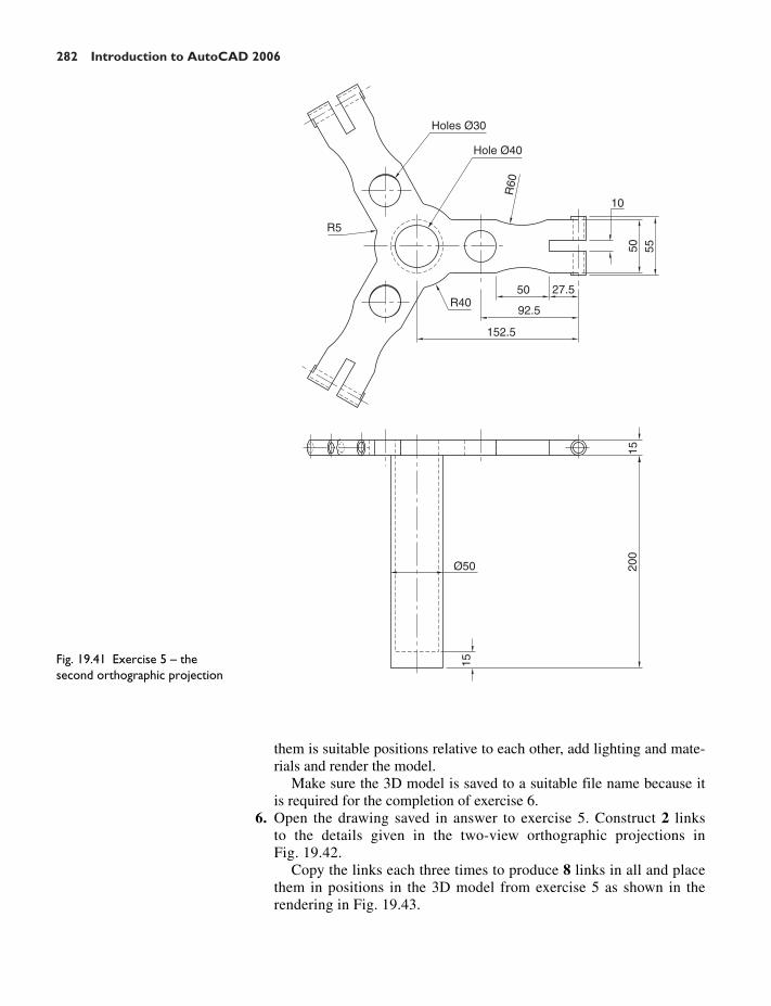
282 Introduction to AutoCAD 2006
Holes Ø30
Hole Ø40
R60
10
50 55
50 27.5
92.5
152.5
R40
R5
1520
0
Ø50
15Fig. 19.41 Exercise 5 – thesecond orthographic projection
them is suitable positions relative to each other, add lighting and mate-rials and render the model.
Make sure the 3D model is saved to a suitable file name because itis required for the completion of exercise 6.
6. Open the drawing saved in answer to exercise 5. Construct 2 linksto the details given in the two-view orthographic projections inFig. 19.42.
Copy the links each three times to produce 8 links in all and placethem in positions in the 3D model from exercise 5 as shown in therendering in Fig. 19.43.

Editing 3D solid models 283
Fig. 19.43 Exercise 6
10
85 65
10
Fillets are R2
Hole Ø10 Ø15
15
Fig. 19.42 Exercise 6 – the twolinks

284
CHAPTER 20
Other features of 3D modelling
Aims of this chapter
1. To give a further example of placing raster images in an AutoCADdrawing.
2. To give examples of the use of the Profile tool to obtain profile-onlydrawings from 3D models.
3. To give examples of methods of printing or plotting not given in previouschapters.
4. To give examples of the use of polygonal viewports.
Raster images in AutoCAD drawings
Example – Raster image in a drawing (Fig. 20.5)
This example shows the raster file rendering.bmp of the 3D modelconstructed to the details given in the drawing in Fig. 20.1.
Ø5
Ø10
90
4050
40
5Ø20
Ø30
Hole Ø50 Ø60
10
40
5
Ø30
Holes Ø20
180Fig. 20.1 Example – Rasterimage in a drawing – details
Raster images are graphics images such as those taken from filesending with the file extensions *.bmp, *.pcx, *.tif and the like. Thetypes of graphics files which can be inserted into AutoCAD drawingscan be seen by first clicking on Raster Image . . . in the Insert drop-down menu (Fig. 20.2), which brings the Select Image File dialog(Fig. 20.3) on screen. In the dialog click the arrow to the right of theFiles of type field and the popup list which appears lists the types ofgraphics files which can be inserted into AutoCAD drawings. Suchgraphics files can be used to describe in 3D the details shown in 2D bya technical drawing.

Other features of 3D modelling 285
4. Zoom the shaded model to a suitable size and press the Print Scr keyof the keyboard.
5. Open the Windows Paint application and click Edit in the menu bar,followed by another click on Paste in the drop-down menu. The wholeAutoCAD screen which includes the Gouraud shaded 3D assembledmode appears.
6. Click the Select tool icon in the toolbar of Paint and window the 3Dmodel. Then click Copy in the Edit drop-down menu.
7. Click New in the File drop-down menu, followed by a click on No inthe warning window which appears.
8. Click Paste in the Edit drop-down menu. The shaded 3D modelappears. Click Save As . . . from the File drop-down menu and savethe bitmap to a suitable file name – in this example – rendering.bmp.
9. Open the orthographic projection drawing in AutoCAD.10. Open the Select Image File and from the file list select render-
ing.bmp (Fig. 20.3). Another dialog (Image) opens (Fig. 20.4)showing the name of the raster image file. Click the OK button ofthe dialog and a series of prompts appear at the command linerequesting position and scale of the image. Enter appropriateresponses to these prompts and the image appears in position in theorthographic drawing (Fig. 20.5).
Fig. 20.2 Selecting RasterImage . . . from the Insertdrop-down menu
Fig. 20.3 The Select Image Filedialog
1. Construct the 3D model to the shapes and sizes given in Fig. 20.1,working in four layers each of a different colour.
2. Place in the SW Isometric view.3. Shade the 3D model using Gouraud Shading from the Shade
sub-menu of the View drop-down menu.

286 Introduction to AutoCAD 2006
Notes
1. It will normally be necessary to enter a scale in response to the promptlines otherwise the raster image may appear very small on screen. If itdoes it can be zoomed anyway.
2. Place the image in position in the drawing area. In Fig. 20.5 the ortho-graphic projections have been placed within a margin and a title blockhas been added.
Fig. 20.4 Example – Rasterimage in a drawing – theImage dialog
Fig. 20.5 Example – Rasterimage in a drawing
The Profile tool
The Profile tool is found in the Solids toolbar (Fig. 20.6). Its purpose is tocreate profile-only drawings from 3D solid drawings.
Fig. 20.6 The Profile tool iconfrom the Solids toolbar

Other features of 3D modelling 287
First example – Profile (Fig. 20.10)
1. Construct a 3D solid model drawing to the details given in Fig. 20.7.
Holes Ø20 C'bore Ø30 10 deepR20
4090
25
R6
R5
R8
R60
140R20
30
5
Fig. 20.7 First example – Profile – orthographic projection
Fig. 20.8 First example – Profile –the mirrored 3D models
2. In the UCS *FRONT* plane copy the 3D model and mirror one of thecopies to, in effect, turn it upside down (Fig. 20.8). Go back to theUCS *WORLD* plane.
3. Place the 3D model in one of the 3D Views isometric views.4. Change to a PSpace screen with a click on the Layout1 tab.5. Click the Cancel button of the Page Setup dialog which appears.6. Either enter ms (MSpace) at the command line or click the PAPER
button in the status bar to turn the PSpace screen into a MSpace screen.7. Either click the Profile tool icon in the Solids toolbar, or enter solprof
at the command line.The command line shows:
Command: enter ms (Model Space) right-clickMSPACE Regenerating model.Command: enter solprof right-clickSelect objects: window the two models 2 foundSelect objects: right-clickDisplay hidden profile lines on separate layer [Yes/No] �Yes�:
right-clickProject profile lines onto a plane [Yes/No] �Y�: right-clickDelete tangential edges [Yes/No] �Yes�: right-click2 solids selectedCommand:

288 Introduction to AutoCAD 2006
Note
Profile-only views can only be created in Layout (Pspace) screens.
Second example – Profile (Fig. 20.11)
Working to the same procedures as those shown for the first example, openthe 3D model drawing of the first example (page 284) and create a profile-only view of the model. The only difference is that when selecting objects,the drawing must be windowed because there are 16 objects in the model.
Printing/Plotting
Hardcopy (prints or plots on paper) from a variety of AutoCAD drawingsof 3D models can be obtained. Some of this variety has already beenshown on pages 234–236 of Chapter 16.
First example – Printing/Plotting (Fig. 20.14)
If an attempt is made to print a multiple viewport screen with all viewportdrawings appearing in the plot, only the current viewport will be printed.To print or plot all viewports:
1. Open a four-viewport screen of the assembled 3D model shown in thefirst example (page 284).
Fig. 20.9 First example – Profile –turn all layers off except PV-2EO
Fig. 20.10 First example – Profile
8. Click the arrow to the right of the Layers field and turn all layers offexcept that with a name commencing PV – in this example this is PV-2E0 (Fig. 20.9). The 3D models appear in profile-only views (Fig. 20.10).

Other features of 3D modelling 289
Fig. 20.12 First example –Printing/Plotting – renamingthe Layout1 tab
Fig. 20.11 Second example –Profile
2. Make a new layer vports of colour yellow. Make the layer vportscurrent.
3. Right-click on the Layout1 tab and click Rename in the menu whichappears. Then in the Rename Layout dialog which comes to screen,enter a new name in the Name field. Click the OK button and theLayout1 tab is renamed (Fig. 20.12).
4. Click the renamed Layout tab. The screen changes to a PSpace layoutwith the Page Setup Layer1 dialog on top. In the dialog select theprinter or plotter to be used by clicking the Plot Device tab and select-ing the required printer/plotter from the Name popup list, followed byclicking the Layout Settings tab and selecting the required sheet sizefrom the Paper Size popup list. Click the OK button of the dialog.

290 Introduction to AutoCAD 2006
5. The Paper Space layout appears with the current viewport outlined inyellow (the colour of the vports layer). Using the Erase tool erase theviewport with a click on its boundary line. The viewport and its contentsdisappear.
6. At the command line:
Command: enter mv (Mview) right-clickMVIEWSpecify corner of viewport or [ON/OFF/Shadeplot/Lock/Object/
Polygonal/Restore/2/3/4]: enter 4 right-clickSpecify first corner of viewport or [Fit] �Fit�: right-clickRegenerating model.Command:
And four viewports appear with the 3D model drawing in each.7. Make sure the variable UCSFOLLOW is off (0) in each viewport.8. Click the PAPER button in the status bar to change the screen to
Model Space.9. Make each viewport in turn current with a click in its area and using
the 3D Views tools, make the top left viewport a Top view, the topright viewport a Right view, the bottom left viewport a Front viewand the bottom right viewport a SW Isometric view.
10. In each viewport in turn Zoom the model drawing to a suitable size.11. Click the MODEL tab to change the screen to a Paper Space layout.12. Click the Plot tool icon in the Standard toolbar (Fig. 20.13). A Plot
dialog appears.13. Check that the printer/plotter is correct and the paper size is also correct.14. Click the Full Preview button. The full preview of the plot appears
(Fig. 20.14).
Fig. 20.14 First example –Printing/Plotting
Fig. 20.13 The Plot tool iconfrom the Standard toolbar
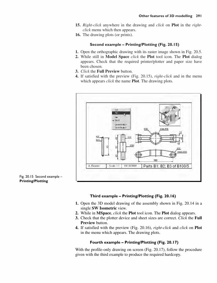
Other features of 3D modelling 291
15. Right-click anywhere in the drawing and click on Plot in the right-click menu which then appears.
16. The drawing plots (or prints).
Second example – Printing/Plotting (Fig. 20.15)
1. Open the orthographic drawing with its raster image shown in Fig. 20.5.2. While still in Model Space click the Plot tool icon. The Plot dialog
appears. Check that the required printer/plotter and paper size havebeen chosen.
3. Click the Full Preview button.4. If satisfied with the preview (Fig. 20.15), right-click and in the menu
which appears click the name Plot. The drawing plots.
Fig. 20.15 Second example –Printing/Plotting
Third example – Printing/Plotting (Fig. 20.16)
1. Open the 3D model drawing of the assembly shown in Fig. 20.14 in asingle SW Isometric view.
2. While in MSpace, click the Plot tool icon. The Plot dialog appears.3. Check that the plotter device and sheet sizes are correct. Click the Full
Preview button.4. If satisfied with the preview (Fig. 20.16), right-click and click on Plot
in the menu which appears. The drawing plots.
Fourth example – Printing/Plotting (Fig. 20.17)
With the profile-only drawing on screen (Fig. 20.17), follow the proceduregiven with the third example to produce the required hardcopy.

292 Introduction to AutoCAD 2006
Fig. 20.16 Third example –Printing/Plotting
Fig. 20.17 Fourth example –Printing/Plotting
Polygonal viewports (Fig. 20.18)
The example to illustrate the construction of polygonal viewports is basedupon exercise 7 (page 298). When the 3D model for this exercise has beencompleted in Model Space:
1. Make a new layer Yellow of colour yellow and make this layer current.2. Click the Layout1 tab. Cancel the Page Setup dialog which appears.

Other features of 3D modelling 293
3. Erase the viewport with a click on its bounding line. The outline andits contents are erased.
4. At the command line:
Command: enter mv right-click[prompts]: enter 4 right-click[prompts]: right-clickRegenerating model.Command:
And the model appears in a four-viewport layout.5. Make sure the variable UCSFOLLOW is OFF in each viewport.6. Click the PAPER button in the status bar to turn it to MODEL. With
a click in each viewport in turn and using the 3D Views settings, setviewports in Front, Right, Top and SW Isometric views respectively.
7. Zoom each viewport to All.8. Click the MODEL button to turn back to PAPER.9. Enter mv at the command line which shows:
Command: enter mv right-clickMVIEW[prompts]: enter p (Polygonal) right-clickSpecify start point: In the top right viewport pick one corner for a
squareSpecify next point or [Arc/Close/Length/Undo]: pick next corner for
the squareSpecify next point or [Arc/Close/Length/Undo]: pick next corner
for the squareSpecify next point or [Arc/Close/Length/Undo]: enter c (Close)
right-clickRegenerating model.Command:
And a square viewport outline appears in the top right viewportwithin which is a copy of the model.
10. Repeat in each of the viewports with different shapes of polygonalviewport outlines (Fig. 20.18).
11. Click the PAPER button to change to MODEL.12. In each of the polygonal viewports make a different isometric view.
In the bottom right viewport change the view using the 3D Orbittool.
13. Turn the layer Yellow off. The viewport borders disappear.14. The Plot Preview appears (Fig. 20.19). Plot the screen.
Exercises
1. Fig. 20.20 shows a polyline for each of the four objects from which thesurface shown in the illustration of a Gouraud shaded surface wasobtained. Construct the surface and shade with Gouraud shading(Fig. 20.21).

294 Introduction to AutoCAD 2006
Fig. 20.18 Polygonal viewports –plot preview
Fig. 20.19 Polygonal viewports –plot preview after turning the layerYellow off
80 80 80 80
2020
Fig. 20.20 Exercise 1 – the plinefor each of the four objects

Other features of 3D modelling 295
Fig. 20.21 Exercise 1
Fig. 20.22 Exercise 2
Ø80 Ø
100
Hole Ø80
904020
40 250
R50
R50
R15
R12017
0Fig. 20.23 Exercise 2 – details ofshapes and sizes
3. A partial front view of a stand is shown by a profile-only drawing(Fig. 20.24). From the details given in the drawing in Fig. 20.25,construct a 3D model drawing of the stand. Using appropriate lightingand material render the 3D model which has been constructed.
4. Construct an assembled 3D model drawing, working to the details givenin Fig. 20.26. When the drawing has been constructed, disassemble theparts as shown in the given profile-only drawing. Then construct theprofile-only drawing in Fig. 20.27.
2. Working to the sizes given in Fig. 20.23, construct an assembled3D model drawing of the spindle in its two holders and render(Fig. 20.22).

296 Introduction to AutoCAD 2006
Fig. 20.24 Exercise 3 – profile-only drawing
R15
Hole Ø15
15 deep
135
30
Ø90
15
45°
200
Ø45
Ø35
5020
102.515 deep
R15
Hole Ø20
M10 SQ 8060
45 20 20 20 10
R5
Ø10
R20
Ø20Ø40Ø50
Holes Ø10
10
10Hole Ø40
R10
10
Ø40
20
SQ
80
Fig. 20.26 Exercise 4 – details ofshapes and sizes
Fig. 20.25 Exercise 3
5. The surface model for this exercise was constructed from threeedgesurf surfaces, working to the suggested objects for the surfaceas shown in Fig. 20.30. The third surface objects in each case are leftto your discretion. Fig. 20.28 gives the completed surface model.Fig. 20.29 shows the three surfaces separated from each other.

Other features of 3D modelling 297
Fig. 20.27 Exercise 4
Fig. 20.28 Exercise 5
Fig. 20.29 Exercise 5 – surfacesseparated
Object 1
Object 1
Object 2
Object 2
Object 3
Object 4
Object 3Object 4
Object 1from its
front
Object 3from its
frontFig. 20.30 Exercise 5 – objects foredgesurf surface model
6. Working to the details shown in Fig. 20.31, construct a 3D modelof the assembly, with the parts in their correct positions relative toeach other. Then separate the parts as shown in the profile-onlydrawing in Fig. 20.32. When the 3D model is complete add suitablelighting and materials and render the result.
7. Working to the details shown in Fig. 20.33, construct an exploded3D model of the parts of the handle and when completed construct aprofile-only drawing from your model.

298 Introduction to AutoCAD 2006
R15
R140
R180120
160
R25
SQ 20 6515
125
70
Holes Ø10
15
Hole Ø50
Ø70
R120
4515 105 290
SQ 20 Ø50Ø50
Ø50
55
215
Fig. 20.31 Exercise 6 – detailsdrawing
Fig. 20.32 Exercise 6 – profile-only drawing
Hexagonal slot
Ø160Ø20
Ø120
Ø30Hole Ø25
Ø40 Ø60
20 30
Chamfers 5 × 5
35 110
10Keyway
5 × 5
Ø15R5
10
60
45Fig. 20.33 Exercise 7 – detailsdrawing

Other features of 3D modelling 299
Fig. 20.34 Exercise 7 – renderings
Two renderings of 3D models of the rotating handle are shownin Fig. 20.34 – one with its parts assembled and the other with theparts in an exploded position relative to each other.

300
CHAPTER 21
Internet tools
Aim of this chapter
The purpose of this chapter is to introduce the tools which are availablein AutoCAD 2006, which make use of facilities available on the WorldWide Web .
Emailing drawings
As with any other files which are composed of data, AutoCAD drawingscan be sent by email as attachments. If a problem of security of the draw-ings is involved, they can be encapsulated with a password as the drawingsare saved prior to being attached in an email. To encrypt a drawing witha password, click Tools in the Save Drawing As dialog and from the popuplist which appears click Security Options . . . (Fig. 21.1). Then in theSecurity Options dialog which appears (Fig. 21.2) enter a passwordin the Password or phrase to open this drawing field, followed by a clickon the OK button. The drawing then cannot be opened until the password
Fig. 21.1 Selecting SecurityOptions . . . in the SaveDrawing As dialog
Fig. 21.2 Entering a password inthe Security Options dialog

Internet tools 301
is entered in the Password dialog (Fig. 21.3) which appears when anattempt is made to open the drawing by the person receiving the email.
There are many reasons why drawings may require to be passwordencapsulated in order to protect confidentiality of the contents of drawings.
Fig. 21.3 The Password dialogappearing when a password-encrypted drawing is about to beopened
Example – creating a web page (Fig. 21.5)
To create a web page which includes AutoCAD drawings, left-click Publishto Web . . . from the File drop-down menu. A series of Publish to Webdialogs appear (Fig. 21.4). After making entries in the dialogs which comeon screen after each Next button is clicked, the Preview of the resultingweb page such as that shown in Fig. 21.5 (which can be saved as an *.htmfile) appears. A double-click in any of the thumbnail views and an InternetExplorer page appears showing the selected drawing in full (Fig. 21.6).
In this example the thumbnails are from DWF files (Design Web For-mat files). If a web page includes DWF files they can be opened in theAutodesk DWF Composer which is part of the AutoCAD 2006 softwarepackage. Fig. 21.7 shows a DWF file opened in the DWF Composer.
Fig. 21.4 One of the Publish toWeb dialogs

302 Introduction to AutoCAD 2006
Fig. 21.5 The web page resultingfrom completing the Publish toWeb series of dialogs
Fig. 21.6 The web page resultingfrom a double-click on a thumb nail
Browsing the Web
There are several ways in which Autodesk web pages can be opened fromAutoCAD 2006. A click on Help in the menu bar followed by anotherclick on Autodesk Website in the drop-down menu (Fig. 21.8) andthe Autodesk web page appears on screen (Fig. 21.9). As an example, a

Internet tools 303
Fig. 21.9 The Autodesk web page
Fig. 21.8 Autodesk Website inthe Help drop-down menu
Fig. 21.10 Selecting Browse theWeb from the Web toolbar
selection of other items in the sub-menu brought down with a click onAdditional Online Resources brings up other Autodesk web pages.
Selecting Browse the Web from the Web toolbar (Fig. 21.10) alsobrings up an Autodesk web page.
Fig. 21.7 A DWF file opened inthe AutoCAD DWFComposer

304 Introduction to AutoCAD 2006
The eTransmit tool
Click eTransmit . . . in the File drop-down menu and the Create Trans-mittal dialog appears (Fig. 21.11). The transmittal shown in this example isthe drawing on screen at the time. Fill in details as necessary and click theOK button and a zip file is formed from the drawing file (Fig. 21.12). Thiszip file is easier and quicker to email than the drawing file. The AutoCADdrawing can be obtained by unzipping the zip file at the receiving end.
Fig. 21.12 The zip file createdfrom the Create Transmittaldialog
Fig. 21.11 The CreateTransmittal dialog

305
CHAPTER 22
Design and AutoCAD 2006
Ten reasons for using AutoCAD
1. A CAD software package such as AutoCAD 2006 can be used toproduce any form of technical drawing.
2. Technical drawings can be produced much more speedily usingAutoCAD than when working manually – probably as much as tentimes as quickly when used by skilled AutoCAD operators.
3. Drawing with AutoCAD is less tedious than drawing by hand – featuressuch as hatching, lettering, adding notes, etc. are easier, quicker andindeed more accurate.
4. Drawings or parts of drawings can be moved, copied, scaled, rotated,mirrored and inserted into other drawings without having to redraw.
5. AutoCAD drawings can be saved to a file system without necessarilyhaving to print the drawing. This can save the need for large drawingstorage areas.
6. The same drawing or part of a drawing need never be drawn twice,because it can be copied or inserted into other drawings with ease. Abasic rule when working with AutoCAD is: Never draw the samefeature twice.
7. New details can be added to drawings or be changed within drawingswithout having to mechanically erase the old details.
8. Dimensions can be added to drawings with accuracy, reducing thepossibility of making errors.
9. Drawings can be plotted or printed to any scale without having toredraw.
10. Drawings can be exchanged between computers and/or emailedaround the world without having to physically send the drawing.
The place of AutoCAD 2006 in designing
The contents of this book are designed to help only those who have limited(or no) knowledge and skills of the construction of technical drawingsusing AutoCAD 2006. However it needs to be recognised that the impactof modern computing on the methods of designing in industry has beenimmense. Such features as analysis of stresses, shear forces, bendingforces and the like can be carried out more quickly and accurately usingcomputing methods. The storage of data connected with a design andthe ability to recover the data speedily are carried out much easily usingcomputing methods than prior to the introduction of computing.
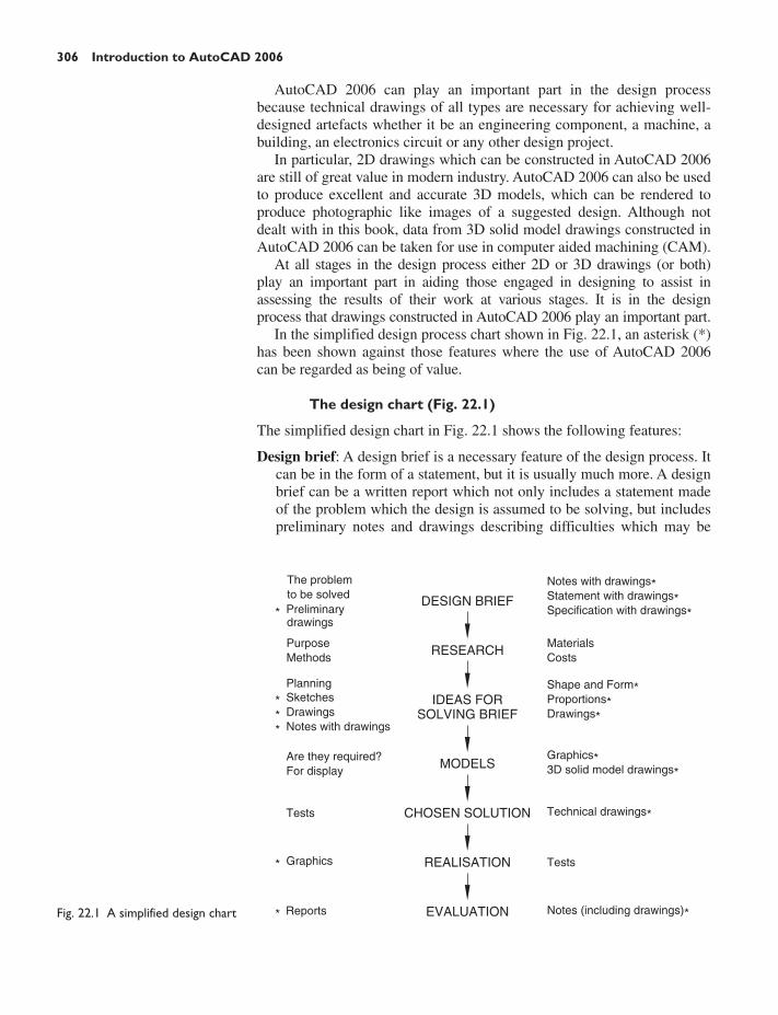
306 Introduction to AutoCAD 2006
AutoCAD 2006 can play an important part in the design processbecause technical drawings of all types are necessary for achieving well-designed artefacts whether it be an engineering component, a machine, abuilding, an electronics circuit or any other design project.
In particular, 2D drawings which can be constructed in AutoCAD 2006are still of great value in modern industry. AutoCAD 2006 can also be usedto produce excellent and accurate 3D models, which can be rendered toproduce photographic like images of a suggested design. Although notdealt with in this book, data from 3D solid model drawings constructed inAutoCAD 2006 can be taken for use in computer aided machining (CAM).
At all stages in the design process either 2D or 3D drawings (or both)play an important part in aiding those engaged in designing to assist inassessing the results of their work at various stages. It is in the designprocess that drawings constructed in AutoCAD 2006 play an important part.
In the simplified design process chart shown in Fig. 22.1, an asterisk (*)has been shown against those features where the use of AutoCAD 2006can be regarded as being of value.
The design chart (Fig. 22.1)
The simplified design chart in Fig. 22.1 shows the following features:
Design brief: A design brief is a necessary feature of the design process. Itcan be in the form of a statement, but it is usually much more. A designbrief can be a written report which not only includes a statement madeof the problem which the design is assumed to be solving, but includespreliminary notes and drawings describing difficulties which may be
Fig. 22.1 A simplified design chart
Notes with drawings*Statement with drawings*Specification with drawings*
MaterialsCosts
Shape and Form*Proportions*Drawings*
Graphics*3D solid model drawings*
Notes (including drawings)*
Technical drawings*
Tests
DESIGN BRIEF
RESEARCH
IDEAS FORSOLVING BRIEF
MODELS
CHOSEN SOLUTION
REALISATION
EVALUATION
PurposeMethods
The problemto be solved
*
Preliminary drawings
Are they required?For display
Tests
*
Graphics
* Reports
*
Sketches
*
Drawings
*
Notes with drawings
Planning

Design and AutoCAD 2006 307
encountered in solving the design and may include charts, drawings,costings, etc. to emphasise some of the needs in solving the problem forwhich the design is being made.
Research: The need to research the various problems which may arise whendesigning is often much more demanding than that shown in the chart(Fig. 22.1). For example the materials being used may require extensiveresearch as to costing, stress analysis, electrical conductivity, difficultiesin machining or in constructional techniques and other such features.
Ideas for solving the brief: This is where technical and other drawingand sketches play an important part in designing. It is only afterresearch that designers can ensure the design brief will be fulfilled.
Models: These may be constructed models in materials representing theactual materials which have been chosen for the design, but in addition3D solid model drawings, such as those which can be constructed inAutoCAD 2006, can be of value. Some models may also be made inthe materials from which the final design is to be made so as to allowtesting of the materials in the design situation.
Chosen solution: This is where the use of drawings constructed inAutoCAD 2006 are of great value. 2D and 3D drawings come intotheir own here. It is from such drawings that the final design will bemanufactured.
Realisation: The design is made. There may be a need to manufacture anumber of the designs in order to enable evaluation of the design to befully assessed.
Evaluation: The manufactured design is tested in situations where it isliable to be placed in use. Evaluation will include reports and noteswhich could include drawings with suggestions for amendments to theworking drawings from which the design was realised.
Enhancements in AutoCAD 2006
Notes on some of the enhancements of AutoCAD 2006 over the previousreleases of AutoCAD include the following. It should be noted that detailsof some of these are not described in this introductory book.
1. The introduction of DYN – Dynamic Input. If the DYN button is seton in the status bar, as the cursor is moved under mouse control the tipsshow distance, angle and the next prompt according to the tool is use.
2. Two new commands have been introduced. Commandlinehide hidesthe command palette from the screen. A warning dialog appearsinforming the operator that some commands may not be available.The second is commandline which is used to bring the commandpalette on screen. When the command palette is hidden, DynamicInput can be used in a larger drawing area.
3. Windowing is coloured. Windowing from top-left to bottom-rightgives a window coloured blue. Windowing from bottom-left to top-right gives a window coloured green.
4. Objects are highlighted as they are picked or selected.

5. New tools (commands) include Join (Modify toolbar), Gradient(Draw toolbar) and Arc Length and Jogged (Dimension toolbar).
6. Changes in the tooltips of icons for some tools, particularly thosewhich bring up dialogs – three dots (. . .) after the name of the tool.
7. Many variations in drop-down menus, mainly in the form of includ-ing tool icons against tool names in the menus.
8. Many changes to the format of dialogs.9. Some changes in the command line prompts and their sequences.
10. Changes to the methods of creating web pages.11. DWF files can be used more efficiently.12. An updated DWF Viewer is now available. Renamed DWF Com-
poser.13. Updating of the methods of creating web pages.14. Some set variables have become obsolete. New set variables intro-
duced.15. Methods of using both dynamic and multiple text input have been
enhanced.16. Hatching has been enhanced.17. Dimensioning has been enhanced.18. Object snap is available for 3D modelling.19. The formation of sheet sets has been enhanced.20. Toolbars and palettes can be locked.21. A 3D DWF feature is now included.22. A New Features Workshop is made available from the Help drop-
down menu.
System requirements for running AutoCAD 2006
Operating system: Windows XP Professional, Windows XP Home orWindows 2000.Microsoft Internet Explorer 6.0.Processor: Pentium III 800 Mhz.RAM: At least 128 MB.Monitor screen: 1024 � 768 VGA with True Colour as a minimum.Hard disk: A minimum of 300 MB.
308 Introduction to AutoCAD 2006

309
APPENDIX A
Printing/Plotting
Introduction
Some suggestions for printing/plotting of AutoCAD drawings havealready been given (pages 234 to 236). Plotters or printers can be selectedfrom a wide range and are used for printing or plotting drawingsconstructed in AutoCAD 2006. The example given in this appendix hasbeen from a print using one of the default printers connected to thecomputer I am using. However if another plotter or printer is connected tothe computer, its driver can be set by first opening the Windows ControlPanel and with a double-click on the Autodesk Plotter Manager iconthe Plotters dialogs appears (Fig. A.1).
Fig. A.1 The Plotters window
Double-click on the Add-A-Plotter Wizard icon and the first of theAdd Plotter series of dialogs appears (Fig. A.2). Click the Next button
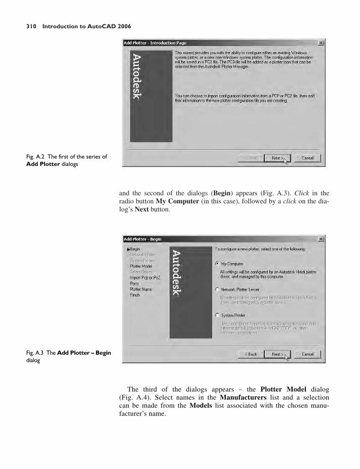
310 Introduction to AutoCAD 2006
and the second of the dialogs (Begin) appears (Fig. A.3). Click in theradio button My Computer (in this case), followed by a click on the dia-log’s Next button.
The third of the dialogs appears – the Plotter Model dialog(Fig. A.4). Select names in the Manufacturers list and a selectioncan be made from the Models list associated with the chosen manu-facturer’s name.
Fig. A.2 The first of the series ofAdd Plotter dialogs
Fig. A.3 The Add Plotter – Begindialog

Printing /Plotting 311
There are several more dialogs in the series in which selections have tobe made before completing the setting up of a printer or plotter for theprinting of AutoCAD drawings.
Notes
1. AutoCAD drawings can be printed from the default printers alreadyinstalled in the Windows system of the computer on which AutoCAD2006 is loaded.
2. Plots or prints from drawings constructed in AutoCAD 2006 can bemade from either Model Space or Paper Space.
An example of a printout
1. Either select Plot . . . with a click on its tool icon in the Standardtoolbar (Fig. A.5) or from the File drop-down menu (Fig. A.6). ThePlot dialog appears (Fig. A.7).
2. There are two parts of the Plot dialog. Fig. A.7 shows the main part. Aclick on the right pointing arrow at the bottom right-hand corner of thedialog opens the second part (Fig. A.8).
3. Select an appropriate printer or plotter from the Printer/plotter list.Then select the correct paper size from the Paper size popup list.Then select what is to be printed/plotted from the What to plot popuplist – in the example shown this is Display. Then click the Preview . . .button.
4. A preview of the drawing to be printed/plotted appears (Fig. A.9). Ifsatisfied with the preview, right-click and from the menu which
Fig. A.4 The Add Plotter –Plotter Model dialog
Fig. A.5 The Plot tool icon in theStandard toolbar
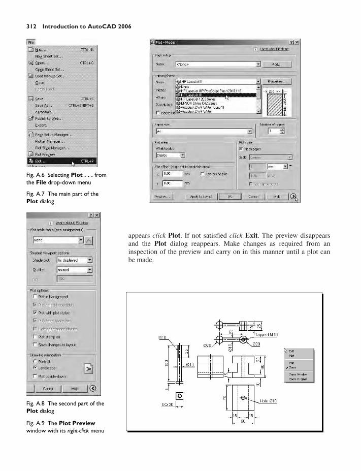
appears click Plot. If not satisfied click Exit. The preview disappearsand the Plot dialog reappears. Make changes as required from aninspection of the preview and carry on in this manner until a plot canbe made.
312 Introduction to AutoCAD 2006
Fig. A.6 Selecting Plot . . . fromthe File drop-down menu
Fig. A.7 The main part of thePlot dialog
Fig. A.8 The second part of thePlot dialog
Fig. A.9 The Plot Previewwindow with its right-click menu

APPENDIX B
List of tools
Introduction
AutoCAD 2006 allows the use of over 300 tools. Some operators preferusing the word “commands”, although command as an alternative to toolis not in common use today. The majority of these tools are described inthis list. Many of the tools described here have not been used in this book,because this book is an introductory text designed to initiate readers intothe basic methods of using AutoCAD 2006. It is hoped the list willencourage readers to experiment with those tools not described in thebook. The abbreviations for tools which can be abbreviated are includedin brackets after the tool name. Tool names can be entered in upper orlower case.
A list of 2D tools is followed by a list of 3D tools. Internet tools aredescribed at the end of this listing.
2D tools
About – Brings the About AutoCAD bitmap on screenAppload – Brings the Load/Unload Applications dialog to screenAdcenter (dc) – Brings the DesignCenter palette on screenAlign (al) – Aligns objects between chosen pointsArc (a) – Creates an arcArea – States in square units the area selected from a number of pointsArray (ar) – Creates Rectangular or Polar arrays in 2DAse – Brings the dbConnect Manager on screenAttdef – Brings the Attribute Definition dialog on screenAttedit – Allows editing of attributes from the Command lineAudit – Checks and fixes any errors in a drawingBhatch (h) – Brings the Boundary Hatch dialog on screenBlock – Brings the Block Definition dialog on screenBmake (b) – Brings the Block Definition dialog on screenBmpout – Brings the Create Raster File dialogBoundary (bo) – Brings the Boundary Creation dialog on screenBreak (br) – Breaks an object into partsCal – Calculates mathematical expressionsChamfer (cha) – Creates a chamfer between two entitiesChprop (ch) – Brings the Properties window on screen
313

314 Introduction to AutoCAD 2006
Circle (c) – Creates a circleCommandline – Brings back the command palette after it has been hidden
by commandlinehideCommandlinehide – Hides the command paletteCopy (co) – Creates a single or multiple copies of selected entitiesCopyclip (Ctrl�C) – Copies a drawing or part of a drawing for inserting
into a document from another applicationCopylink – Forms a link between an AutoCAD drawing and its appearance
in another application such as a word processing packageCustomize – Brings the Customize dialog to screen, allowing the
customisation of toolbars, palettes, etc.Dblist – Creates a database list in a Text window for every entity in a
drawingDdattdef (at) – Brings the Attribute Definition dialog to screenDdatte (ate) – Edits individual attribute valuesDdatext – Brings the Attribute Extraction dialog on screenDdcolor (col) – Brings the Select Color dialog on screenDdedit (ed) – The Text Formatting dialog box appears on selecting textDdim (d) – Brings the Dimension Style Manager dialog box on screenDdinsert (i) – Brings the Insert dialog on screenDdmodify – Brings the Properties window on screenDdosnap (os) – Brings the Drafting Settings dialog on screenDdptype – Brings the Point Style dialog on screenDdrmodes (rm) – Brings the Drafting Settings dialog on screenDdunits (un) – Brings the Drawing Units dialog on screenDdview (v) – Brings the View dialog on screenDel – Allows a file (or any file) to be deletedDim – Starts a session of dimensioningDimension tools – The Dimension toolbar contains the following tools:
Linear, Aligned, Arc Length, Ordinate, Radius, Jogged, Diameter,Angular, Quick Dimension, Baseline, Continue, Quick Leader,Tolerance, Center Mark, Dimension Edit, Dimension Edit Text,Update and Dimension Style
Dim1 – Allows the addition of a single dimension to a drawingDist (di) – Measures the distance between two points in coordinate unitsDivide (div) – Divides an entity into equal partsDonut (do) – Creates a donutDsviewer – Brings the Aerial View window on screenDtext (dt) – Creates dynamic text. Text appears in drawing area as it is
enteredDxbin – Brings the Select DXB File dialog on screenDxfin – Brings the Select File dialog on screenDxfout – Brings the Save Drawing As dialog on screenEllipse (el) – Creates an ellipseErase (e) – Erases selected entities from a drawingExit – Ends a drawing session and closes AutoCAD 2006Explode (x) – Explodes a block or group into its various entitiesExplorer – Brings the Windows Explorer on screen
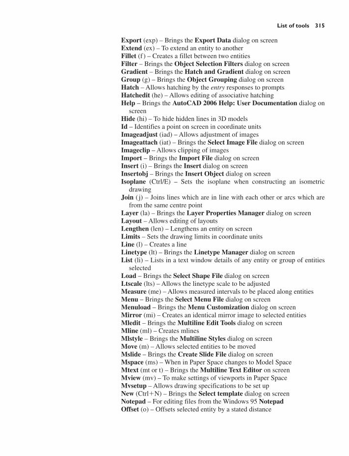
List of tools 315
Export (exp) – Brings the Export Data dialog on screenExtend (ex) – To extend an entity to anotherFillet (f) – Creates a fillet between two entitiesFilter – Brings the Object Selection Filters dialog on screenGradient – Brings the Hatch and Gradient dialog on screenGroup (g) – Brings the Object Grouping dialog on screenHatch – Allows hatching by the entry responses to promptsHatchedit (he) – Allows editing of associative hatchingHelp – Brings the AutoCAD 2006 Help: User Documentation dialog on
screenHide (hi) – To hide hidden lines in 3D modelsId – Identifies a point on screen in coordinate unitsImageadjust (iad) – Allows adjustment of imagesImageattach (iat) – Brings the Select Image File dialog on screenImageclip – Allows clipping of imagesImport – Brings the Import File dialog on screenInsert (i) – Brings the Insert dialog on screenInsertobj – Brings the Insert Object dialog on screenIsoplane (Ctrl/E) – Sets the isoplane when constructing an isometric
drawingJoin ( j) – Joins lines which are in line with each other or arcs which are
from the same centre pointLayer (la) – Brings the Layer Properties Manager dialog on screenLayout – Allows editing of layoutsLengthen (len) – Lengthens an entity on screenLimits – Sets the drawing limits in coordinate unitsLine (l) – Creates a lineLinetype (lt) – Brings the Linetype Manager dialog on screenList (li) – Lists in a text window details of any entity or group of entities
selectedLoad – Brings the Select Shape File dialog on screenLtscale (lts) – Allows the linetype scale to be adjustedMeasure (me) – Allows measured intervals to be placed along entitiesMenu – Brings the Select Menu File dialog on screenMenuload – Brings the Menu Customization dialog on screenMirror (mi) – Creates an identical mirror image to selected entitiesMledit – Brings the Multiline Edit Tools dialog on screenMline (ml) – Creates mlinesMlstyle – Brings the Multiline Styles dialog on screenMove (m) – Allows selected entities to be movedMslide – Brings the Create Slide File dialog on screenMspace (ms) – When in Paper Space changes to Model SpaceMtext (mt or t) – Brings the Multiline Text Editor on screenMview (mv) – To make settings of viewports in Paper SpaceMvsetup – Allows drawing specifications to be set upNew (Ctrl�N) – Brings the Select template dialog on screenNotepad – For editing files from the Windows 95 NotepadOffset (o) – Offsets selected entity by a stated distance

316 Introduction to AutoCAD 2006
Oops – Cancels the effect of using EraseOpen – Brings the Select File dialog on screenOptions – Brings the Options dialog to screenOrtho – Allows ortho to be set ON/OFFOsnap (os) – Brings the Drafting Settings dialog to screenPagesetup – Brings either the Page Setup Model or the Page Setup –
Layout1 dialog to screen for setting print/plot parametersPan (p) – Drags a drawing in any directionPbrush – Brings Windows Paint on screenPedit (pe) – Allows editing of polylines. One of the options is Multiple
allowing continuous editing of polylines without closing the commandPline (pl) – Creates a polylinePlot (Ctrl�P) – Brings the Plot dialog to screenPoint (po) – Allows a point to be placed on screenPolygon (pol) – Creates a polygonPolyline (pl) – Creates a polylinePreferences (pr) – Brings the Options dialog on screenPreview (pre) – Brings the print/plot preview box on screenProperties – Brings the Properties palette on screenPsfill – Allows polylines to be filled with patternsPsout – Brings the Create Postscript File dialog on screenPurge (pu) – Purges unwanted data from a drawing before saving to fileQsave – Saves the drawing file to its current name in AutoCAD 2006Quickcalc (qc) – Brings the QUICKCALC palette to screenQuit – Ends a drawing session and closes down AutoCAD 2006Ray – A construction line from a pointRecover – Brings the Select File dialog on screen to allow recovery of
selected drawings as necessaryRectang (rec) – Creates a pline rectangleRedefine – If an AutoCAD command name has been turned off by
Undefine, Redefine turns the command name back onRedo – Cancels the last UndoRedraw (r) – Redraws the contents of the AutoCAD 2006 drawing areaRedrawall (ra) – Redraws the whole of a drawingRegen (re) – Regenerates the contents of the AutoCAD 2006 drawing
areaRegenall (rea) – Regenerates the whole of a drawingRegion (reg) – Creates a region from an area within a boundaryRename (ren) – Brings the Rename dialog on screenReplay – Brings the Replay dialog on screen from which bitmap image
files can be selectedRevcloud – Forms a cloud-like outline around objects in a drawing to
which attention needs to be drawnSave (Ctrl�S) – Brings the Save Drawing As dialog box on screenSaveas – Brings the Save Drawing As dialog box on screenSaveimg – Brings the Save Image dialog on screenScale (sc) – Allows selected entities to be scaled in size – smaller or
larger

List of tools 317
Script (scr) – Brings the Select Script File dialog on screenSetvar (set) – Can be used to bring a list of the settings of set variables
into an AutoCAD Text windowShape – Inserts an already loaded shape into a drawingShell – Allows MS-DOS commands to be enteredSketch – Allows freehand sketchingSolid (so) – Creates a filled outline in triangular partsSpell (sp) – Brings the Check Spelling dialog on screenSpline (spl) – Creates a spline curve through selected pointsSplinedit (spe) – Allows the editing of a spline curveStats – Brings the Statistics dialog on screenStatus – Shows the status (particularly memory use) in a Text windowStretch (s) – Allows selected entities to be stretchedStyle (st) – Brings the Text Style dialog on screenTablet (ta) – Allows a tablet to be used with a pointing deviceTbconfig – Brings the Customize dialog on screen to allow configuration
of a toolbarText – Allows text from the Command line to be entered into a drawingThickness (th) – Sets the thickness for the Elevation commandTilemode – Allows settings to enable Paper SpaceTolerance – Brings the Geometric Tolerance dialog on screenToolbar (to) – Brings the Toolbars dialog on screenTrim (tr) – Allows entities to be trimmed up to other entitiesType – Types the contents of a named file to screenUCS – Allows selection of UCS (User Coordinate System) facilitiesUndefine – Suppresses an AutoCAD command nameUndo (u) (Ctrl�Z) – Undoes the last action of a toolView – Brings the View dialog on screenVplayer – Controls the visibility of layers in Paper SpaceVports – Brings the Viewports dialog on screenVslide – Brings the Select Slide File dialog on screenWblock (w) – Brings the Create Drawing File dialog on screenWmfin – Brings the Import WMF File dialog on screenWipeout – Forms a polygonal outline within which all crossed parts of
objects are erasedWmfopts – Brings the Import Options dialog on screenWmfout – Brings the Create WMF dialog on screenXattach (xa) – Brings the Select Reference File dialog on screenXline – Creates a construction lineXref (xr) – Brings the Xref Manager dialog on screenZoom (z) – Brings the zoom tool into action
3D tools
3darray – Creates an array of 3D models in 3D space3dface (3f) – Creates a 3- or 4-sided 3D mesh behind which other features
can be hidden3dmesh – Creates a 3D mesh in 3D space

318 Introduction to AutoCAD 2006
3dorbit – Allows a continuous movement and other methods of manipu-lation of 3D models on screen
3ddistance – Allows the controlling of the distance of 3D models fromthe operator
3dorbit (3do) – Allows methods of manipulating 3D models on screen3dorbitctr – Allows further and a variety of other methods of manipulation
of 3D models on screen3dpan – Allows the panning of 3D models vertically and horizontally on
screen3dsin – Brings the 3D Studio File Import dialog on screen3dsout – Brings the 3D Studio Output File dialog on screenAlign – Allows selected entities to be aligned to selected points in 3D spaceAmeconvert – Converts AME solid models (from Release 12) into
AutoCAD 2000 solid modelsBox – Creates a 3D solid boxCone – Creates a 3D model of a coneCylinder – Creates a 3D cylinderDducs (uc) – Brings the UCS dialog on screenEdgesurf – Creates a 3D mesh surface from four adjoining edgesExtrude (ext) – Extrudes a closed polylineInterfere – Creates an interference solid from selection of several solidsIntersect (in) – Creates an intersection solid from a group of solidsLight – Brings the Lights dialog on screenMatlib – Brings the Materials Library dialog on screenMirror3d – Mirrors 3D models in 3D space in selected directionsMview (mv) – When in Paper Space brings in Model Space objectsPface – Allows the construction of a 3D mesh through a number of selected
verticesPlan – Allows a drawing in 3D space to be seen in plan (UCS World)Pspace (ps) – Changes Model Space to Paper SpaceRender – Brings the Render dialog on screenRevolve (rev) – Forms a solid of revolution from outlinesRevsurf – Creates a solid of revolution from a plineRmat – Brings the Materials dialog on screenRpref (rpr) – Brings the Rendering Preferences dialog on screenRulesurf – Creates a 3D mesh between two entitiesScene – Brings the Scenes dialog on screenSection (sec) – Creates a section plane in a 3D modelShade (sha) – Shades a selected 3D modelSlice (sl) – Allows a 3D model to be cut into several partsSolprof – Creates a profile from a 3D solid model drawingSphere – Creates a 3D solid model sphereStlout – Saves a 3D model drawing in ASCII or binary formatTorus (tor) – Allows a 3D torus to be createdUcs – Allows settings of the UCS planeVports – Brings the Viewports dialog on screenSubtract (su) – Subtracts one 3D solid from anotherTabsurf – Creates a 3D solid from an outline and a direction vector

List of tools 319
Union (uni) – Unites 3D solids into a single solidVpoint – Allows viewing positions to be set from x,y,z entriesWedge (we) – Creates a 3D solid in the shape of a wedge
Internet tools
Browse the Web – Brings Autodesk home page from the Internet on screenEtransmit – Brings the Create Transmittal dialog to screenPublish – Brings the Publish to Web dialog to screen

APPENDIX C
Some of the set variables
Introduction
AutoCAD 2006 is controlled by a large number of variables (over 440 innumber), the settings of many of which are determined when makingentries in dialogs. Others have to be set at the command line. Some areread-only variables which depend upon the configuration of AutoCAD2006 when it originally loaded into a computer (default values).
A list of those set variables follows which are of interest in that theyoften require setting by entering figures or letters at the command line.To set a variable, enter its name at the command line and respond to theprompts which arise.
To see all set variables, enter set (or setvar) at the command line:
Command: enter set right-clickSETVAR Enter variable name or ?: enter ?Enter variable name to list �*�: right-click
And a Text window opens showing a first window with a list of the first ofthe variables. To continue with the list press the Return key whenprompted and at each press of the Return key another window opens.
Some of the set variables
ANGDIR – Sets angle direction. 0 counterclockwise; 1 clockwiseAPERTURE – Sets size of pick box in pixelsBLIPMODE – Set to 1 marker blips show; set to 0 no blipsCOMMANDLINE – Opens the command line paletteCOMMANDLINEHIDE – Closes the command line palette
Note
DIM variables – There are over 70 variables for setting dimensioning, butmost are in any case set in the Dimension Style dialog or as dimension-ing proceeds. However one series of the Dim variables may be of interest:
DMBLOCK – Sets a name for the block drawn for an operator’s ownarrowheads. These are drawn in unit sizes and saved as required
DIMBLK1 – Operator’s arrowhead for first end of lineDIMBLK2 – Operator’s arrowhead for other end of line
320

Some of the set variables 321
DRAGMODE – Set to 0 no dragging; set to 1 dragging on; set to 2automatic dragging
DRAG1 – Sets regeneration drag sampling. Initial value is 10DRAG2 – Sets fast dragging regeneration rate. Initial value is 25DYNMODE – Turns DYN on/offFILEDIA – Set to 0 disables Open and Save As dialogs; set to 1 enables
these dialogsFILLMODE – Set to 1 hatched areas are filled with hatching. Set to 0
hatched areas are not filled. Set to 0 plines are not filledGRIPS – Set to 1 and grips show. Set to 0 grips do not showMBUTTONPAN – Set to 0 no right-click menu with the Intellimouse.
Set to 1 Intellimouse right-click menu onMIRRTEXT – Set to 0 text direction is retained; set to 1 text is mirroredPELLIPSE – Set to 0 creates true ellipses; set to 1 polyline ellipsesPICKBOX – Sets selection pick box height in pixelsPICKDRAG – Set to 0 selection windows picked by two corners; set to 1
selection windows are dragged from corner to cornerRASTERPREVIEW – Set to 0 raster preview images not created with
drawing. Set to 1 preview image createdSHORTCUTMENU – For controlling how right-click menus show: 0 all
disabled; 1 default menus only; 2 edit mode menus; 4 command modemenus; 8 command mode menus when options are currently available.Adding the figures enables more than one option
SURFTAB1 – Sets mesh density in the M direction for surfaces generatedby the Surfaces tools
SURFTAB2 – Sets mesh density in the N direction for surfaces generatedby the Surfaces tools
TEXTFILL – Set to 0 True Type text shows as outlines only; set to 1True Type text is filled
TILEMODE – Set to 0 Paper Space enabled; set to 1 tiled viewports inModel Space
TOOLTIPS – Set to 0 no tool tips; set to 1 tool tips enabledTPSTATE – Set to 0 the Tool Palettes window is inactive. Set to 1 the
Tool Palettes window is activeTRIMMODE – Set to 0 edges not trimmed when Chamfer and Fillet are
used; set to 1 edges are trimmedUCSFOLLOW – Set to 0 new UCS settings do not take effect; set to 1
UCS settings follow requested settingsUCSICON – Set OFF UCS icon does not show; set to ON it shows

APPENDIX D
Computing terms
This glossary contains some of the more common computing terms.
Application – The name given to software packages which perform thetasks such as word processing, Desktop Packaging, CAD, etc.
ASCII – The American National Standard Code for Information Inter-change. A code which sets bits for characters used in computing.
Attribute – Text appearing in a drawing, sometimes linked to a block.Autodesk – The American company which produces AutoCAD and other
CAD software packages.Baud rate – A measure of the rate at which a computer system can
receive information (measured in bits per second).Bios – Basic Input–Output System. The chip in a PC that controls the
operations performed by the hardware (e.g. disks, screen, keyboard etc.).Bit – Short for binary digit. Binary is a form of mathematics that uses
only two numbers: 0 and 1. Computers operate completely on binarymathematics.
Block – A group of objects or entities on screen that have been linkedtogether to act as one unit.
Booting up – Starting up a computer to an operating level.Bus – An electronic channel that allows the movement of data around a
computer.Byte – A sequence of 8 bits.C – A computer programming language.Cache – A section of memory (can be ROM or RAM) which holds
data that is being frequently used. Speeds up the action of disks andapplications.
CAD – Computer-aided design. The term should not be used to meancomputer-aided drawing.
CAD/CAM – Computer-aided design and manufacturing.Cd-ROM – Computer disc read only memory. A disk system capable of
storing several hundred MB of data – commonly 640 MB. Data canonly be read from a CD-ROM, not written to it.
Chips – Pieces of silicon (usually) that drive computers and into whichelectronic circuits are embedded.
Command Line – In AutoCAD 2006, the Command Line is a window inwhich commands are entered from the keyboard and which containsthe prompts and responses to commands.
Clock speed – Usually measured in MHz (Megahertz) – this is the measureof the speed at which a computer processor works.
322

Computing terms 323
Clone – Refers to a PC that functions in a way identical to the originalIBM PC.
CMOS – Complimentary metal oxide semiconductor. Often found asbattery-powered chips which control features such as the PC’s clockspeed.
Communications – Describes the software and hardware that allowcomputers to communicate.
Compatibility – Generally used as a term for software or programs ableto run on any computer that is an IBM clone.
Coprocessor – A processor chip in a computer which runs in tandem withthe main processor chip and can deal with arithmetic involving manydecimal points (floating-point arithmetic). Often used in CAD systemsto speed up drawing operations.
CPU – Central processing unit. The chip that drives a PC.Data – Information that is created, used or stored on a computer in digital
form.Database – A piece of software that can handle and organise large
amounts of information.DesignXML – An Autodesk XML computer program for representing
design data over the Internet.Dialog box – A window that appears on screen in which options may be
presented to the user, or requires the user to input informationrequested by the current application.
Directories – The system in MS-DOS for organising files on disk. Could becompared with a folder (the directory) containing documents (the files).
Disks – Storage hardware for holding data (files, applications, etc.). Thereare many types: the most common are hard disks (for mass storage),floppy disks (less storage) and CD-ROMs (mass storage).
Display – The screen allowing an operator to see the results of his work ata computer.
DOS – Disk operating system. The software that allows the computer toaccess and organise stored data. MS-DOS (produced by the MicrosoftCorporation) is the DOS most widely used in PCs.
DTP – Desktop publishing. DTP software allows for the combination oftext and graphics into page layouts which may then be printed.
Entity – A single feature in graphics being drawn on screen – a line, acircle, a point. Sometimes linked together in a block, when the blockacts as an entity.
EMS – Expanded memory specification. RAM over and above the originallimit of 640 KB RAM in the original IBM PC. PCs are now being builtto take up to 128 (or even more) MB RAM.
File – Collection of data held as an entity on a disk.Fixed disk – A hard disk that cannot usually be easily removed from the
computer as distinct from floppy disks which are designed to be easilyremovable.
Floppy disk – A removable disk that stores data in magnetic form. Theactual disk is a thin circular sheet of plastic with a magnetic surface,hence the term “floppy”. It usually has a firm plastic case.

324 Introduction to AutoCAD 2006
Flyout – A number of tool icons which appear when a tool icon whichshows a small arrow is selected from a toolbar.
Formatting – The process of preparing the magnetic surface of a disk toenable it to hold digital data.
ftp – File Transfer Protocol. An Internet protocol used to fetch a requiredresource from the World Wide Web (www) server.
Giga – Means 1,000,000,000. In computer memory terms really 1000 MB(megabytes) – actually 1,073,741,824 bytes because there are 1024 bytesin a kilobyte (KB).
GUI – Graphical user interface. Describes software (such as Windows)which allows the user to control the computer by representing functionswith icons and other graphical images.
Hardcopy – The result of printing (or plotting) text or graphics on topaper or card.
Hard disk – A disk, usually fixed in a computer, which rotates at highspeed and will hold large amounts of data often up to 1 gigabyte.
Hardware – The equipment used in computing: the computer itself,disks, printers, monitor, etc.
HTML – HyperText Markup Language. A computer language for settingup pages which can be sent via the Internet
http – HyperText Transfer Protocol. An Internet protocol used to fetch arequired resource from the World Wide Web (www) server.
Hz (hertz) – The measure of 1 cycle per second. In computing terms,often used in millions of Hertz – (megahertz or MHz) as a measure ofthe clock-speed.
IBM – International Business Machines. An American computer manu-facturing company – the largest in the world.
Intel – An American company which manufactures the processing chipsused in the majority of PCs.
Internet – A network of computers linked in a worldwide system bytelephone.
Joystick – A small control unit used mainly in computer games. SomeCAD systems use a joystick to control drawing on screen.
Kilo – Means 1000. In computing terms 1KB (kilobyte) is 1024 bytes.LAN – Local area network. Describes a network that typically links PCs
in an office by cable where distances between the PCs is small.LED – Light emitting diode.Library – A set of frequently used symbols, phrases or other data on disk
that can be easily accessed by the operator.Light pen – Used as a stylus to point directly at a display screen sensitive
to its use.Memory – Any medium (such as RAM or ROM chips) that allows the
computer to store data internally that can be instantly recalled.Message box – A window containing a message to be acted on which
appears in response when certain tools or commands are selected.MHz – Megahertz – 1,000,000 Hz (cycles per second).Microcomputer – A PC is a microcomputer; a minicomputer is much
larger and a mainframe computer is larger still. With the increase in

Computing terms 325
memory possible with a microcomputer, the term seems to be droppingout of use.
Microsoft – The American company which produces Windows andMS-DOS software.
MIPS – Millions of instructions per second. A measure of a computer’sspeed – it is not comparable with the clock speed as measured inMHz, because a single instruction may take more than a cycle toperform.
Monitor – Display screen.Mouse – A device for controlling the position of an on-screen cursor
within a GUI such as Windows.MS-DOS – Microsoft Disk Operating System.Multitasking – A computer that can carry out more than one task at a time
is said to be multitasking. For example in AutoCAD Windows printingcan be carried out “in the background”, while a new drawing is beingconstructed.
Multi-user – A computer that may be used by more than one operator.Networking – The joining together of a group of computers allowing
them to share the same data and software applications. LANs andWANs are examples of the types of networks available.
Object – A term used in CAD to describe an entity or group of entitiesthat have been linked together.
Operating System – Software, and in some cases hardware, that allows theuser to operate applications software and organise and use data stored on acomputer which allow the hardware of a computer to operate applicationsoftware.
PC – Personal computer. Should strictly only be used to refer to an IBMclone, but is now in general use.
Pixels – The individual dots on a monitor display.Plotter – Produces hardcopy of, for instance, a drawing produced on a
computer by moving a pen over a piece of paper or card.Printer – There are many types of printer: dot-matrix, bubble-jet and
laser are the most common. Allows material produced on a computer(graphics and text) to be output as hardcopy.
Processor – The operating chip of a PC. Usually a single chip, such asthe Intel 80386, 80486 or Pentium chip.
Programs – A set of instructions to the computer that has been designedto produce a given result.
RAM – Random access memory. Data stored in RAM is lost when thecomputer is switched off, unless previously saved to a disk.
RGB – Red, green, blue.ROM – Read only memory. Refers to those chips from which the data
stored can be read, but to which data can not be written. The data on aROM is not lost when a computer is switched off.
Scanner – Hardware capable of being passed over a document or drawing,reading the image into a computer.
Software – Refers to any program or application that is used and run on acomputer.

326 Introduction to AutoCAD 2006
SQL – Structured query language. A computer programming languagefor translating and transferring data between an application such asAutoCAD and a database.
Tools – Tools are usually selected from icons appearing in toolbars. Atool represents a command.
Toolbar – Toolbars contain a number icons, representing tools.Tooltip – When a tool is selected by a left-click on its icon, a small box
appears (a Tool Tip) carrying the name of the tool.UNIX – A multiuser, multitasking operating system (short for UNICS:
uniplexed information and computing systems).URL – Uniform Resource Locator.URL address – It has three parts; for example, in the address http://
www.autodesk.com/acaduser, http:// describes the service;www.autodesk.com is the Internet address; acaduser is the location atthe Internet address.
VDU – Visual display unit.Vectors – Refers to entities in computer graphics which are defined by
the coordinates of end points of each part of the entity.VGA – Video graphics array. Screen displays with resolution of up to
640 � 480 pixels in 256 colours. SVGA (Super VGA) will allowresolutions of up to 1024 � 768 pixels.
Virtual memory – A system by which disk space is used as if it wereRAM to allow the computer to function as if more physical RAM werepresent. It is used by AutoCAD (and other software), but can slowdown a computer’s operation.
WAN – Wide area network. A network of computers that are a largedistance apart, often communicating by telephone.
Warning box – A window containing a warning or request which the usermust respond to, which appears when certain circumstances are met orcertain actions are made.
WIMP – Windows, icons, mice and pointers. A term used to describesome GUIs.
Windows – An area of the computer screen within which applicationssuch as word processors may be operated.
Workstation – Often used to refer to a multiuser PC, or other system,used for the purposes of CAD (or other applications).
WORM – Write once read many. An optical data storage system thatallows blank optical disks to have data written onto them only once.
www – World Wide Web.WYSIWYG – What you see is what you get. What is seen on the screen
is what will be printed.

*.bmp files 284*.dwf 163*.dwt files 10*.dxf 147*.eps files 145*.mpr files 222*.pcx files 284*.tif files 2842D coordinates 92D objects in 3D space 2472D outlines for 3D models 1763D Array tool 2113D coordinates 103D Face tool 1753D Mesh tool 2633D model libraries 2073D modelling 1733D models – modifying 2073D models 10, 2743D objects 1843D Orbit toolbar 2333D polar array 2123D rectangular array 2113D space 2403D Studio 1503D surface meshes 2553D Views 3, 1753D Views menu 240
A3 sheet 56A4_template.dwt 62Abbreviations 31Abbreviations Modify tools 80Absolute coordinates 18Absolute entry 28Acadiso.dwt 61Acadiso.dwt template 10Add-A-Plotter Wizard icon 309Add Plotter dialog 311Advanced hatching 124Aerial View windows 52, 54
327
Aligned Dimension tool 88Ambient light 228Angle direction 18Angular dimensions 93ANSI hatching 119Arc Length tool 94Arc tool 31Array dialog 70Array tool 68Associative hatching 121AutoCAD 2006 windows 2AutoCAD drawing template 12, 60AutoCAD text fonts 99Autodesk Website 302Autohide icon 2Autohide right-click menu 2AutoSnap 35, 38
Block Definition dialog 133Blocks 132Boolean operators 190Box tool 184, 258Break tool 76Browse the Web tool 303Browsing the web 302Building drawing 166Buttons 7Buttons in status bar 8
Calling tools 31, 64Chamfer tool 78, 187Check boxes 7Check Spelling dialog 103Checking spelling 102Circle tool 20Clipboard 144Close button 16Close dialog button 6Color Faces tool 273Colour gradient hatching 121Command line 15, 47
Index

Command line dimensions 89Command line sequence 16Command palette 2, 12Commandline variable 42Commandlinehide variable 40Cone tool 18, 258Coordinate system 9Copy Faces tool 271Copy Link tool 143Copy tool 65, 145Copy with Base Point tool 145Counterclockwise rotation 71Create Mass and Area Properties
dialog 222Create Sheet Set dialogs 158Create Transmittal dialog 304Crossing windows 22, 75Cursor hairs 4Customize User Interface 5Cylinder tool 185
Data Exchange Format files 147Deferred tangent 21Design and AutoCAD 2006 305Design chart 306Design Web Format 163DesignCenter 140DesignCenter palette 4, 136Desktop 1Dialog 5, 27Digitiser 3Dimension Edit Text tool 93Dimension Style 56Dimension Style Manager 58Dimension tolerances 95Dimension tools 87Dimensions 87Dimensions from command line 89Dimensions Style Manager 87Distant light 228Dome tool 258Double-click 13Drafting Settings dialog 36, 41Dragging 13Draw drop-down menu 32Draw Order toolbar 2Draw toolbar 1Drawing area 2Drawing template 10, 56Drawing Utilities dialog 137Drop-down menu 27DWF Composer 163, 303
328 Index
DXF files 147DYN 9, 36Dynamic Input 9, 35, 40Dynamic Text 98
Edge tool 263Edgesurf tool 262Edit drop-down menu 143Edit Polyline tool 44Editing dimensions 93Ellipse tool 33Emailing drawings 300End view 106Enhancements in AutoCAD 2006 307Enter key 3Erase tool 21, 64ETransmit tool 304Explode tool 64, 135, 137Export Data dialog 145Extend tool 78External Reference dialog 151External Reference files 150Extrude Faces tool 179, 268
F12 key 40F6 key 16F8 key 19F9 key 16Field 47File formats 143Fillet tool 78, 187First angle projection 108Floating toolbars 5Floor layouts 167Floppy disk 34Flyout 13Fonts – AutoCAD 99Fonts – text 99Fonts – Windows True Type 99Front view 106Function keys 8
Geometrical dimension symbols 98Geometrical toleranced
dimensions 97Gouraud shading 234Grid 8
Hatch and Gradient dialog 110, 122Hatch Pattern Palette 110, 119Hatching – advanced 125Hatching – associative 121

Hatching sectional views 109Hide tool 174Horizontal dimensions 90
Illuminating 3D models 229Image dialog 149, 286Inquiry toolbar 221Insert Block tool 134Insert drop-down menu 148Inserting 3D blocks 207Inserting blocks 134Inserts 132Internet tools 300Intersect tool 178ISO hatching 119ISOLINES variable 181, 255Isometric circle 112Isometric drawing 106
Jogged tool 94Join tool 77
Layer locked 119Layer Properties Manager 59Layers 59, 108, 219Layers toolbar 2, 59Layout format 157Leader dimensions 92Left-click 13Lighting 3D models 229Lights 228Lights dialog 230Limits 15, 56Line tool 15Linear Dimension tool 8Linetypes 60Lineweight 9Links Manager 146Locked layer 119LWT 9
Major axis 32Make Block tool 132, 207Massprop tool 221Materials dialog 231MDE 152Menu bar 3Microsoft Word program 144Minimize button 143Minor axis 32Mirror 3D tool 214Mirror tool 67, 175
Index 329
MIRRTEXT variable 67Model 9MODEL button 235Modify II toolbar 44Modify tool abbreviations 80Modify toolbar 2, 64Modify tools 64Modifying 3D models 207Mouse 3, 16Mouse wheel 3, 56Move Faces tool 269Move tool 71Multiple copy 66Multiple Document
Environment 152Multiple Polyline Edit 46Multiple view printing 236, 288MVIEW 290
New Layer icon 60New Point Light dialog 230
Object 47Object linking and embedding
143Offset Faces tool 270Offset tool 68OLE 143Opening AutoCAD 2006 1Options dialog 4, 38Ortho 9Orthographic projection 106Osnap 9, 35Osnap abbreviations 38Otrack 9
PageMaker program 145Paint program 285Palettes 4Pan 52Pan tool 55PAPER button 235Paper Space 10, 63Password dialog 301Passwords 300Pedit 44Pedit on 3D surfaces 262PELLIPSE variable 47Pick 14Pick box 4Pick button 3Place tool 145

Plan 106Plot dialog 312Plot Preview 312Plot tool 311Plotters dialog 309Point lights 228Polar 9Polar Array 70Polygon tool 42Polygonal viewports 292Polygonal windows 75Polygons 43Polyline Edit tool 44Polyline tool 23Popup list 6, 47Preview area 7Printing 234Printing/plotting 309Printing/plotting 3D model
drawings 288Printouts 311Profile tool 286Prompts 27Properties palette 4Properties toolbar 2Publish to Web dialogs 301Purge dialog 138Purge tool 137
Radio buttons 8Radius Dimension tool 89Raster images 148, 284Rectangle tool 43Rectangular array 68Redo tool 23Region tool 177, 248Regions 177Regions rendering 190Relative coordinates 18Relative entry 28Render dialog 190Render toolbar 174Render tools 228Rendering 190, 228Rendering lighting 228Rendering regions 190Rendering surface models 263Return button 3, 13Return key 27Revolve tool 183Revolved Surface tool 259Right-click 13
330 Index
Right-click menus 14Rotate 3D tool 216Rotate Faces tool 272Rotate tool 71Rotation of objects 71Rubber band 19Ruled Surface tool 261
Save Drawing As dialog 35Saving 3D model drawings 236Saving drawings 34Saving UCS views 247Scale tool 72Section hatching 119Section hatching rules 121Section tool 218Sectional view 108, 220Security Options dialog 300Select File dialog 5Select Image File dialog
148, 285Select template dialog 10Selection windows 80Setting layers 59Setting text 56Shading Modes 234Sheet Set Manager 161Sheet sets 157Shortcut 1SHORTCUTMENU variable 56SHX fonts 99Simple toleranced dimensions 95Site plan 166Slice tool 217Snap 8Solids Editing toolbar 174, 268Solids toolbar 174Spelling 102Sphere tool 185Spotlight 228Standard toolbar 1, 4, 52, 139Status bar 8, 15Stretch tool 75Styles toolbar 2, 87Sub-menus 3Subtract tool 177Surface tools 255Surfaces toolbar 174SURFTAB variables 255Switch selector 3Symbols for geometrical dimensions
98

Symbols for text 100System requirements for AutoCAD
2006 308
Tabs 7Tabulated Surface tool 260Taper Faces tool 270Template 10, 56Template file 60Text 87, 99Text fonts 99Text Formatting dialog 100Text hatching 124Text Style 56Text symbols 100Third angle projection 108Title bar 3, 5Toggling 8Toleranced dimensions 95Tolerances – geometrical 97Tolerances – simple 97Toolbar 47Toolbar menu 5Toolbars 1, 5Tools drop-down
menu 102Tooltip 27Torus tool 187, 259Tracking 19, 28Transparent commands 46Trim tool 73True Type fonts 99Two-button mouse 3
UCS 241UCS dialog 241UCS icon 242UCS II dialog 241UCS planes 243UCS views – saving 247UCSFOLLOW variable 242Undo tool 23Union tool 177Units 12
Index 331
Units dialog 12User Coordinate System 241
Vertical dimensions 90View drop-down menu 197View menu 3Viewpoint Presets dialog 223Viewports 197Viewports dialog 198Views in orthographic projection 106Visual effects 80
Warning windows 16Wblocks 140Web page 301Wedge tool 186Windows 1Windows Excel program 222Windows multi-tasking 3Windows Paint program 285Windows True Type fonts 99WORLD plane 240Write Block dialog 140
Xref Manager dialog 150Xrefs 150X,Y 10XY Plane 240X,Y,Z 10XZ Plane 240
YZ Plane 240
Z coordinate 173Zoom 52Zoom All 52Zoom Center 52Zoom Dynamic 52Zoom Extents 53Zoom Object 53Zoom Previous 53Zoom Realtime 52Zoom Realtime tool 52Zoom Windows 53

This Page is Intentionally Left Blank