Auto-context and Its Application to High-level Vision Tasks

and 3D Brain Image Segmentation

Zhuowen Tu and Xiang BaiLab of Neuro Imaging, University of California, Los Angeles

{ ztu,xiang.bai}@loni.ucla.edu

July 9, 2009

Abstract

The notion of using context information for solving high-level vision and medicalimage segmentation problems has been increasingly realized in the field. However, howto learn an effective and efficient context model, together with an image appearancemodel, remains mostly unknown. The current literature using Markov Random Fields(MRFs) and Conditional Random Fields (CRFs) often involves specific algorithm de-sign, in which the modeling and computing stages are studied in isolation. In thispaper, we propose the auto-context algorithm. Given a set of training images andtheir corresponding label maps, we first learn a classifier on local image patches. Thediscriminative probability (or classification confidence) maps created by the learned clas-sifier are then used as context information, in addition to the original image patches,to train a new classifier. The algorithm then iterates until convergence. Auto-contextintegrates low-level and context information by fusing a large number of low-level ap-pearance features with context and implicit shape information. The resulting discrim-inative algorithm is general and easy to implement. Under nearly the same parametersettings in training, we apply the algorithm to three challenging vision applications:foreground/background segregation, human body configuration estimation, and sceneregion labeling. Moreover, context also plays a very important role in medical/brainimages where the anatomical structures are mostly constrained to relatively fixed po-sitions. With only some slight changes resulting from using 3D instead of 2D features,the auto-context algorithm applied to brain MRI image segmentation is shown to out-perform state-of-the-art algorithms specifically designed for this domain. Furthermore,the scope of the proposed algorithm goes beyond image analysis and it has the potentialto be used for a wide variety of problems in multi-variate labeling.

Keywords: object recognition, image segmentation, context, 3D brain segmentation,discriminative models, Markov random field.

1

1 Introduction

Context and high-level information plays a vital role in object recognition and scene un-

derstanding [2, 31, 48]. Nevertheless, a principled way of learning an effective and efficient

context model, together with an image appearance model, is not available. Many types of

information can be referred to as context: different parts of an object can be context to

each other; different objects in a scene can be each other’s context. For example, a clearly

visible horse’s head may suggest the locations of its tail and leg, which are often occluded.

A car might suggest the existence of a road, and vice versa [18].

From the Bayesian point of view, context information is carried in the joint statistics

of multi-variate in the posterior probability, which is often decomposed into likelihood and

prior. In vision, likelihood and prior often correspond to appearance and shape respectively.

There are many technological hurdles to overcome to build successful vision systems. The

difficulties can be summarized into two main aspects: modeling and computing. (1) Difficulty

in modeling complex appearances– objects in natural images observe complex patterns

and there are many factors contributing to the complexity such as textures (homogeneous

or inhomogeneous), lighting conditions, viewing angles, and occlusions. (2) Difficulty in

learning complicated shapes and configurations. Shape modeling has been one of the most

studied topics in computer vision and medical imaging, and the problem remains mostly

unsolved. (3) Difficulty in computing for the optimal solution.

In vision, models like Markov Random Fields (MRFs) [13] and Conditional Random

Fields (CRFs) [23, 21] have been used to capture the context information. Energy mini-

mization algorithms, such as Belief Propagation (BP) [32, 59], have been widely adopted.

However, these models and algorithms share somewhat similar disadvantages: (1) the choice

of functions used are quite limited so far; (2) they usually rely on a fixed topology with

very limited neighborhood relations; (3) many of them are only guaranteed to obtain the

optimal solution for limited function families. Hidden Markov Models (HMMs) [26] have

been used to study the dependencies of neighboring states, which is in a way similar to

MRFs. HMMs are also limited to short range context information. In Sect. (3.4), we will

provide more insights about why auto-context is effective and compare it against the Belief

Propagation (BP) algorithm.

In this paper, we make an effort to address some of the shortcomings of existing meth-

ods by proposing a new algorithm, auto-context. The algorithm targets the posterior dis-

tribution directly in a supervised manner. Like in the BP algorithm [59], the goal is to

learn/compute the marginals of the posterior, which we also call classification maps for the

2

rest of this paper. Each training image comes with a label map in which every pixel is

assigned with a label of interest. A classifier is first trained to classify every pixel. There

are two types of features for the classifier to choose from: (1) image features computed on

the local image patches and (2) context information from a large number of sites on the

classification maps. In this paper, we use image patches of fixed size 21×21 and 11×11×11

for 2D natural images and 3D MRI images respectively. The size is fixed for all rounds of

the algorithm. For natural images, the initial classification maps are usually uniform, since

we do not know what objects might appear at where a prior. Context features are typically

not selected by the first classifier since they are uninformative. The first trained classifier

produces a new classification map which becomes the input for training the next classifier.

The algorithm iterates to approach the ground truth until convergence. In medical imaging,

we can often use a probabilistic atlas [38] as the initial classification map since the anatom-

ical structures are roughly positioned. In testing, the algorithm follows the same procedure

by applying the sequence of learned classifiers to compute the posterior marginals.

The auto-context algorithm integrates rich image appearance models together with the

context information by learning a series of classifiers. The appearance (likelihood) and the

high-level context and shape information (prior) are seamlessly combined in an implicit way

and the balance between the two is naturally handled. Unlike many energy minimization

algorithms where the modeling and computing stages are separated, auto-context uses the

same procedures in both phases. The training and testing results differ in the generalization

power of the trained algorithm. Auto-context uses deterministic procedures for computing

the marginal distributions. However, it does not make any hard decisions in the process.

Uncertainties are propagated through learned closed-form functions in the classifiers, rather

than by performing sampling or integration. This makes the auto-context algorithm signif-

icantly faster than most existing algorithms. Compared to MRFs and CRFs, auto-context

is not limited to a fixed neighborhood structure. Each pixel/voxel can have support from

a large number of neighbors, either short or long range. It is up to the learning algorithm

to select and fuse them. The classifiers in different stages may choose different support-

ing neighbors to either enhance or suppress the current probability to converge toward the

ground truth.

We demonstrate the auto-context algorithm on challenging high-level vision tasks for

three well-known datasets: horse segmentation in the Weizmann dataset [3], human body

configuration estimation in the Berkeley dataset [29], and scene region labeling in the MSRC

dataset [41]. The results demonstrate significant improvement over many existing algo-

rithms, in terms of both speed and quality. In addition, we apply the algorithm on brain

3

images for both segmenting a single structure (caudate) and performing whole brain seg-

mentation. A thorough comparison is made using many standard metrics and we observe a

large improvement over state-of-the-art algorithms across various domains. The proposed

auto-context framework is general and easy to implement. Its scope goes beyond high-level

vision tasks; indeed, it has the potential to be used for many problems for multi-variate

labeling where joint statistics need to be modeled. This is demonstrated on a typical ma-

chine learning problem, handwritten character recognition [20], and we observe comparable

performance gain with a state-of-the-art algorithm [45].

2 Related work

We discuss related work in two broad areas: 2D image understanding and 3D medical image

segmentation.

2.1 Related 2D image understanding work

There has been a lot of recent work in using context information for object recognition,

scene understanding [18, 41, 35, 46, 54, 15, 42], and tracking [58, 56]. A pioneering work

was proposed by Belongie et al. [2] which used context in shape matching. Hoiem et

al. [18, 17] presented a system combining the interaction between different objects in a

loop as mutual support. Auto-context differs from these works in several aspects: (1) it

has a single objective function to minimize (classification error); (2) local appearances and

context are simultaneously integrated; (3) the training procedure in auto-context is simpler

and more general.

Three approaches directly related to auto-context are: Boosted Random Fields (BRFs) [46],

Mutual Boosting [9], and SpatialBoost [1], which all used boosting to combine the contex-

tual information. However, these algorithms used contextual beliefs as weak learner in the

boosting algorithm. Auto-context is a general algorithm and the classifier of choice is not

limited to boosting. It directly targets the posterior through iterative steps, resulting in a

simpler and more efficient algorithm. Under nearly the same set of parameters in training,

we demonstrate several 2D natural image and 3D medical image applications using the

auto-context algorithm, which are not available in [46, 9, 1].

A feed-forward way of combining context and appearance was proposed in [54] for object

detection. However, their method does not iteratively learn a posterior. More importantly,

their findings led to the conclusion that the performance gain from using context is neg-

ligible (unless the image quality is really poor). Our experimental results in Fig. (4.a)

4

suggest otherwise. One possible reason might be due to their specifically designed context

features. Other groups [35] have also shown that explicit context information improves

region segmentation/labeling results greatly, which matches our conclusions. Compared to

other algorithms that use context [35, 18], it learns an integrated model without the need

for specifying particular types of context. Auto-context also differs from the feed-forward

neural networks [25] in its way of selecting and fusing information from both the original

data and the iteratively updated probability maps.

2.2 Related 3D image segmentation work

The task of segmenting sub-cortical and cortical structures is very difficult, due to their

intrinsic ambiguous patterns. Neuroanatomists often develop and use complicated protocols

[30] in guiding the manual delineation process and these protocols may vary from task to

task. There have been many medical image segmentation algorithms developed in the past.

These algorithms range from shape driven [57, 33], atlas and knowledge based [38], Markov

Random Fields models [10, 34], to classification/learning based approaches [24]. They have

produced encouraging results, although there are some common drawbacks: (1) most of

them assume very simple appearance patterns; (2) many algorithms are slow with very

time-consuming energy minimization steps (e.g. it takes about one day for FreeSurfer [10]

to segment a MRI image); and (3) they usually involve heavy algorithm design (e.g. many

carefully engineered energy terms) which poses a big hurdle for transporting the systems

to other modalities, or even on the same modality but to segment different anatomical

structures.

It was shown in [57] that using a joint prior for the shapes of neighboring brain structures

can improve the segmentation result. Even though context information might play a more

important role in 3D medical image analysis than in 2D natural images, context has been

somewhat under-explored in the medical imaging domain. One possible reason is due to

the difficulty of deriving explicit context information for 3D objects. The proposed auto-

context algorithm has the advantage of fusing a large number of 3D context and implicit

shape features, without the need of worrying about explicit 3D shape representations.

3 Problem formulation

In this section, we present the problem formulation for the auto-context algorithm and

briefly discuss some related algorithms.

5

3.1 Objective

For a 2D image, the input is X = (x(i,j), (i, j) ∈ Λ) where Λ denotes the image lattice. For

an 1D vector, the input can be denoted as X = (x1, ..., xn). For notational simplicity, we

do not distinguish the two and call them both ‘images’. We will use the 1D vector input for

illustration. In training, each imageX comes with a ground truth Y = (y1, ..., yn) where yi ∈{1, ...,K} is the class label for pixel i. The training set is then S = {(Yj ,Xj), j = 1, ...,m}where m denotes the number of training images. The Bayes rule says p(Y |X) = p(X|Y )p(Y )

p(X) ,

where p(X|Y ) and p(Y ) are the likelihood and prior respectively. One possibility is to

search for the optimal solution by maximizing a posterior (MAP),

Y ∗ = arg max p(Y |X) = arg max p(X|Y )p(Y ).

As mentioned before, the main difficulties for the MAP framework come from two aspects.

(1) Modeling: it is very hard to learn accurate p(X|Y ) and p(Y ) for real-world cluttered

images. Both of them have high complexity and usually do not follow independent identical

distributions (i.i.d.). (2) Computing: the combination of the p(X|Y ) and p(Y ) is often non-

regular. Besides many recent advances made in optimization and energy minimization [44],

a general solution still remains out of reach.

Instead of decomposing p(Y |X) into p(X|Y ) and p(Y ), we study the posterior directly.

Moreover, we look at the marginal distribution P = (p1, ...,pn) where pi, as a vector for

discrete labels, denotes the marginal distribution of

p(yi|X) =∫p(yi, Y−i|X)dY−i, (1)

where Y−i refers to the rest of y other than yi. This is seemingly a more challenging task

as it requires integrating out all the dY−i. Next, we discuss how to approach this.

3.2 Traditional classification approaches

A traditional way to approximate eqn. (1) is by treating it as a classification problem.

Usually, a classifier is considered to be translation invariant. The training set becomes

S = {(yji,Xj(Ni)), j = 1, ...,m, i = 1, ..., n}, where m is the number of training images and

n is the number of pixels in each image. For notational simplicity, we assume one training

image since using multiple training images follows the identical procedure.

S = {(yi,X(Ni)), i = 1, ..., n}.

Instead of using the entire image X, the training set includes an image patch centered at

each i, X(Ni). Ni denotes all the pixels in the patch. In the context of boosting algorithms,

6

it was shown [11, 12] that one can learn the discriminative model based on logistic regression

p(y = k|X(N)) =eFk(X(N))

∑Kk=1 e

Fk(X(N)). (2)

Fk(X(N)) =∑T

t=1 αk,t · hk,t(X(N)) is the strong classifier on a weighted sum of selected

weak classifier hk,t for label k. Many other classifiers also output a confidence which can be

turned into an approximated posterior. It is noted that our algorithm is not limited to any

particular choice of classifier and many traditional classifiers can be used, such as CART [4]

or SVM [51]. The learned posterior marginal, p(y = k|X(N)), is a very crude approximation

to eqn. (1) and it only uses context through image patch X(N). Due to this limitation, the

well-known Conditional Random fields (CRFs) algorithms [23, 21] try to explicitly include

the context information by adding another term p(yi1, yi2|X(Ni1),X(Ni2)), where i1 and i2

are the neighbors. Though CRFs have been successfully applied in many applications [21,

22, 36], it still has the limitations similar to those in the MRFs as discussed in Sect. (1).

CRFs still use fixed neighborhood structure with a fairly limited number of connections. The

computing complexity explodes given a large neighborhood (clique) structure. This limits

their modeling capability and only short-range context is used in most cases (the long-range

context model in [22] uses only very sparse connections). Also, it limits their computing

capability since the interactions are slowly propagated through pair-wise relations.

3.3 Auto-context

classifier 1trainingX)|P(y

classifier 2 classifier n

X)|(yP(0) X)|(yP(1) X)|(yP 1)-(nX)|(yP(n)

X

Figure 1: Illustration of the classification map updated at each round for the horse seg-

mentation problem. The blue rectangles represent candidate context locations and the red

rectangles represent selected contexts in training at each stage.

To better approximate the marginals in eqn. (1) by including a large amount of context

information, we propose the auto-context model. As mentioned above, a traditional classifier

7

can learn a classification model based on local image patches, which now we call

P(0) = (p(0)1 , ...,p(0)

n )

where p(0)i is the posterior marginal for each pixel i learned by eqn. (2). We construct a

new training set

S1 = {(yi, (X(Ni),P(0)(i))), i = 1, ..., n}, (3)

where P(0)(i) is the classification map for the training image centered at pixel i. We train

a new classifier, not only on the features from the image patch X(Ni), but also on the

probabilities, P(0)(i), of a large number of context locations. These pixels can be either

near or very far from i. Fig. (1) shows an illustration. It is up to the learning algorithm to

select and fuse important supporting context locations, together with features about image

appearance. Once a new classifier is learned, the algorithm repeats the same procedure

until convergence.

Note that, even the first classifier is trained the same way as the others. We simply

start the probability map from a uniform distribution. Since the uniform distribution

is not informative, the context features are not selected by the first classifier. In certain

applications, such as medical image segmentation, the positions of the anatomical structures

are roughly known, and one can use a probability atlas [38] as the initial P(0). Fig. (2)

outlines the training process of the auto-context algorithm.

Given a set of training images together with their label maps, S = {(Yj , Xj), j = 1..m}: For each image

Xj , construct probability maps P(0)j with uniform distribution on all the labels. For t = 1, ..., T :

• Make a training set St = {(yji, (Xj(Ni),P(t−1)j (i))), j = 1..m, i = 1..n}.

• Train a classifier on both image and context features extracted from Xj(Ni) and P(t−1)j (i)) respec-

tively.

• Use the trained classifier to compute new classification maps P(t)j (i) for each training image Xj .

The algorithm outputs a sequence of trained classifiers for p(n)(yi|X(Ni),P(n−1)(i))

Figure 2: The training procedure of the auto-context algorithm.

3.3.1 Auto-context convergence analysis

The algorithm iteratively updates the marginal distribution to approach

p(n)(yi|X(Ni),P(n−1))→ p(yi|X) =∫p(yi, y−i|X)dy−i. (4)

8

Next, we show that the algorithm is asymptotically approaching p(yi|X) without doing

explicit integration. A more direct link between the two, however, is left for future research.

Theorem 1 The auto-context algorithm (not tied to any particular classifier type) monoton-

ically decreases the training error, ε =∑

i δ(yi �= H(X(i)), where yi is the true label and

H(X(i)) is the output by the classifier.

Proof: We show it in the context of boosting but the proof holds on other classifiers as well.

Again, we consider only one image in the training data and use X(i) to denote X(Ni). In

the AdaBoost algorithm [11], one choice of error function is taken by ε =∑

i e−yiH(X(i))

for yi ∈ {−1,+1}, which can be given an explanation as the log-likelihood model [12]. The

multi-class case can be written in a logistic function as well, as in eqn. (2).

At different steps, we have

εt = −∑

i

log p(t)i (yi) = −

∑i

log p(t)(yi|X(i),P(t−1)(i)), and

εt−1 = −∑

i

log p(t−1)i (yi),

where

p(t)(yi|X(i),P(t−1)(i)) =eF

(t)k (X(i),P(t−1)(i))

∑Kk=1 e

Fk(t)(X(i),P(t−1)(i)). (5)

F(t)k (X(i),P(t−1)(i)) includes a set of weak classifiers selected for label class k. It is straight-

forward to see that we can at least make

p(t)(yi|X(i),P(t−1)(i)) = p(t−1)i (yi)

since the equality can be easily achieved by making

F(t)k (X(i),P(t−1)(i)) = log p(t−1)

i (k).

The boosting algorithm (or almost any valid classifier) chooses a set of F (t)k in minimizing

the total error εt, which should at least do better than p(t−1)i (yi) Therefore,

εt ≤ εt−1. �

When other types of classifiers are used on the error measure, ε =∑

i δ(yi �= H(X(i)).

The proof also holds as long as the classifier can choose the current classification confidence

as input feature. The convergence rate depends on the amount of error reduced εt−1 − εt.Intuitively, the next round of classifier tries to select features both from the appearances and

9

the previous classification maps. A trivial solution is to use the previous probability map for

the classifier. This also shows that the optimal classifier is at a stable point. Of course, this

requires having the feature of its own probability (or classified labels or the error function is

measured on the labels) in the candidate pool, which is not hard to achieve. Note that this

proof does not guarantee convergence to the global optimal solution. However, by fusing

a large number of context information, the algorithm is shown to be effective in practice,

as we demonstrate on many applications. Fig. (1) gives an illustration of the iterations

of auto-context. There have been some debate about the probabilistic explanation for the

boosting algorithms. Nevertheless, we emphasize that the proposed auto-context framework

is not dependent on any particular choice of classifier.

3.3.2 Feature design

In this section, we discuss the two types of features used: (1) image appearance features

and (2) context features.

Image features

The image appearance features include Haar responses on the input image. For the 2D

applications shown in this paper, we use a similar set of Haar features used in [53]. One

reason to use Haar is due to their computational efficiency when computed using integral

images [53]. For color images, we use the L∗u∗v∗ decomposition and compute the Haar

features on three channels separately. Complementary features can collaboratively improve

the performance. For example, histogram of gradient (HOG) features [7] are shown to be

very effective and they are somewhat complementary to the Haar features. In some cases,

the absolute position of a pixel is a good feature as well. It is particularly informative for

medical images where objects have roughly fixed positions. In scene understanding, it is

useful also since sky often appears on the top and road appears on the bottom. In addition,

we can obtain filter responses of different Gabor functions and Canny edge maps at different

scales.

The size for the basic image patch can vary as well. For appearance-based classification,

using a big patch, say, 51×51 will perform slightly better than using a small one, say 21×21.

However, the difference diminishes in the later stages of the auto-context algorithm with

context features included. We tried three different patch sizes, 21×21, 41×41, and 51×51

in the horse segmentation experiment (Sect. (4.1)), and the F-values at the first stage are

respectively 0.78, 080, and 0.80. However, they all reach 0.83 at the fourth stage. We have

a similar observation on the MSRC dataset though the difference in the first stage is bigger,

10

in terms of pixel accuracy: 58.0% using 51×51 versus 50.4% using 21×21 at the first stage,

but they both reach around 77% in the end.

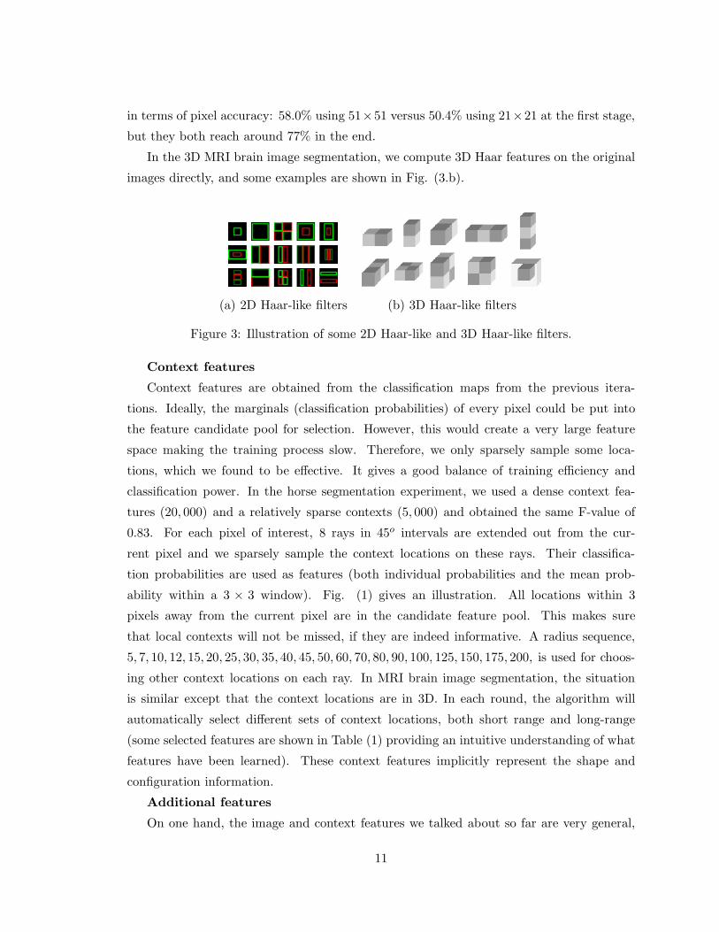
In the 3D MRI brain image segmentation, we compute 3D Haar features on the original

images directly, and some examples are shown in Fig. (3.b).

(a) 2D Haar-like filters (b) 3D Haar-like filters

Figure 3: Illustration of some 2D Haar-like and 3D Haar-like filters.

Context features

Context features are obtained from the classification maps from the previous itera-

tions. Ideally, the marginals (classification probabilities) of every pixel could be put into

the feature candidate pool for selection. However, this would create a very large feature

space making the training process slow. Therefore, we only sparsely sample some loca-

tions, which we found to be effective. It gives a good balance of training efficiency and

classification power. In the horse segmentation experiment, we used a dense context fea-

tures (20, 000) and a relatively sparse contexts (5, 000) and obtained the same F-value of

0.83. For each pixel of interest, 8 rays in 45o intervals are extended out from the cur-

rent pixel and we sparsely sample the context locations on these rays. Their classifica-

tion probabilities are used as features (both individual probabilities and the mean prob-

ability within a 3 × 3 window). Fig. (1) gives an illustration. All locations within 3

pixels away from the current pixel are in the candidate feature pool. This makes sure

that local contexts will not be missed, if they are indeed informative. A radius sequence,

5, 7, 10, 12, 15, 20, 25, 30, 35, 40, 45, 50, 60, 70, 80, 90, 100, 125, 150, 175, 200, is used for choos-

ing other context locations on each ray. In MRI brain image segmentation, the situation

is similar except that the context locations are in 3D. In each round, the algorithm will

automatically select different sets of context locations, both short range and long-range

(some selected features are shown in Table (1) providing an intuitive understanding of what

features have been learned). These context features implicitly represent the shape and

configuration information.

Additional features

On one hand, the image and context features we talked about so far are very general,

11

Table 1: Description of some features selected by the auto-context algorithm in the second

stage for the MSRC image labeling task. Since there are multiple labels, each image has

n discriminative probability maps on every label. For example, p(building) denotes the

probability map for each pixel being of the building class. In the second column, the first

selected feature for some classes is given where [(), ()] denotes a rectangle of the top-left

and bottom-right corner w.r.t. the current pixel of interest. We give the description of the

fourth selected features, many of which show contextual information. Some contexts are

used to do enhancement, e.g. the body context for the face class; some others might be

doing suppression, e.g. the building context for the sheep class. The figures in the right

demonstrates the features for face and bike respectively.

and they can be directly applied to many applications. On the other hand, in image

understanding and medical imaging, there are often domain specific variables (sometimes

hidden) to the solutions. The understanding and explicit inference of these variables are

likely to further improve the performance of a system. For example, using the geometric

cues [16] about the 3D world facilitates a better understanding of 2D images [17]. In the

3D brain image segmentation task, we engaged an explicit generative model to extract an

adaptive atlas first. We observe around 10 ∼ 20% performance gain on a large MRI dataset

(> 500 images) over the baseline algorithm (no context); using the auto-context algorithm

on top of all these features gives further 5 ∼ 10% improvemnt (the 20% performance gain

is due to the complementariness of generative and discriminative models and a detailed

discussion can be found in [27]). This is evident that using informative cues improves the

performance of the auto-context algorithm. We leave the study of exploring other cues

about domain specific variables for future research.

12

3.4 Understanding auto-context

We first take a look at the Belief Propagation algorithm [32, 59] since it also works on the

marginal distribution. For certain directed graphs, BP can find the global optimal. For

graphs with loops, BP computes an approximation. For a model on a graph

p(Y ) =1Z

∏(i,j)

ψ(yi, yj)∏

i

φi(yi)

where Z is the normalization constant, ψ(yi, yj) is the pair-wise relation between sites i and

j, and φi(yi) is a unary term. The BP algorithm [59] computes the belief (marginal) pi(yi)

by

pi(yi) =1Zφi(yi)

∏j∈N(i)

mji(yi), (6)

where mji(xi) are the messages from j to i,

mij(yj)←∑yi

φi(yi)ψi,j(yi, yj)∏

k∈N(i)\jmki(yi). (7)

Similarly, the auto-context algorithm updates the marginal distribution by eqn. (5). The

major differences between BP and auto-context are: (1) In BP, every pair of ψi,j(yi, yj)

on all possible labels needs to be evaluated and integrated in eqn. (7). Therefore, BP can

only work with a limited number of neighborhoods to keep the computational burden under

check. For auto-context, we evaluate a sequence of learned classifiers, F (t)k (X(i),P(t−1)(i)),

which are computed discriminatively based on a set of selected features. Therefore, auto-

context can afford to look at a much longer range of support and it is up to the learning

algorithm to select and fuse the most informative context and appearance information.

Note that, there is no integration between the pair yi and yj. (2) BP works on a fixed

graph structure and the update rule is the same. Auto-context learns different classifiers on

different sets of features at different stages, which allows it to make use of the best available

information each time. In the experiments, we will compare different choices of learning

classifiers, e.g. using a fixed one, or separating the context prior from the likelihood. We

show that the auto-context setting works the best. (3) In BP, there are often separate stages

to design the graphical model and to learn ψ(yi, yj) and φi(yi). Auto-context is designed

to learn the posterior marginal directly and its inference stage follows identical steps to

the learning phase. However, BP has the advantage that it uses the same message passing

rule for different forms of pi(yi) in eqn. (6), whereas auto-context learns a different set of

classifiers for different tasks.

13

A question one might ask is: “How different is learning a recursive model p(t)(yi|Xi,P(t−1)(i))

and learning p(yi|X) directly?”. A classifier can be trained by using the entire image X

rather than an image patch X(i). A major issue is that p(yi|X) should be a marginal

distribution by integrating out the other i’s as shown in eqn. (1). The correlation between

different pixels needs to be taken into account, which is done by learning one classifier for

p(yi|X). A key concept here is about knowledge representation and propagation. An image

is composed of many different objects. Objects and their parts often locally observe certain

degrees of regularity, and it is much more effective to gather information locally and propa-

gate it than trying to solve everything in one shot. The possible configurations of different

objects or even the same object with different parts are too numerous to learn effectively.

It would also result in a feature space too big for a classifier to handle, which would lead

to overfitting.

Wolf and Bileschi [54] suggested that using label context might achieve the same effect

as using image appearance context in object detection; moreover, for both types of context

their improvements were small. We conducted an experiment to train a system with image

appearance, instead of the probabilities, for the pixels sparsely sampled on the rays, as

suggested in [54]. Our results are shown in Fig. (4.a) and the conclusions differ significantly

from [54] in two aspects: (1) having a much enlarged appearance context pool actually de-

grades performance (as opposed to using only local appearance features); (2) label context,

computed using our auto-context algorithm, greatly improves the segmentation/labeling

result.

There have been many algorithms that have attempted to integrate context [2, 35, 18,

46, 1]. The auto-context algorithm makes an attempt to recursively select and fuse context

information, as well as appearance, in a unified framework. The first trained classifier

is based purely on the local appearance; objects with strong appearance cues are often

correctly classified even after the first round. These probabilities then start to influence

their neighbors, especially if there are strong correlations between them.

4 Experiments

We perform experimental studies in three areas: (1) 2D natural image understanding, (2)

handwritten OCR recognition, and (3) 3D MRI brain image segmentation. For 2D image

understanding, we illustrate the auto-context algorithm on three challenging tasks: horse

segmentation, human body configuration estimation, and scene parsing/labeling. In these

three tasks, the system uses a nearly identical parameter setting, including the number of

14

weak classifiers and the stopping criterion. For brain imaging applications, we show both

single structure (caudate) segmentation and whole brain segmentation.

The procedures described in the auto-context algorithm are generic. However, there are

several important implementation issues and a detailed discussion will help to better un-

derstand the algorithm. Next, we highlight some critical points and empirical observations,

which apply to all experiments reported in this section.

1. Choice of classifier: Auto-context uses a sequence of classifiers, and thus, the clas-

sifier quality influences overall performance. Since we use a large number of candidate

features (around ten thousand) in the image understanding case, boosting appears to

be a good choice. It has many appealing properties: a natural feature selection and

fusion process; can deal with a large number of features on a considerable amount

of training data; features do not have to be normalized; it can be efficiently trained

and used. SVMs can also be used, as shown in the OCR case in Sect. (4.2), but

they are better suited when the number of features is relatively small. In the horse

segmentation example, we try SVM classifier also. The F-values by the first and sec-

ond stages of a SVM-based auto-context are respectively 0.54 and 0.75, whereas a

boosting-based auto-context achieves 0.78 and 0.82 respectively. This confirms that

auto-context is not tied to any specific choice of classifier; however, as we can see,

due to the feature selection and fusion capability of different types of classifier, dif-

ferent choices of the base classifier do have an impact on the overall performance.

Using decision-tree (typically 2- or 3- level) as the weak classifier significantly outper-

forms decision-stump-based boosting [12]. In the experiments, each boosted classifier

selects and fuses 100 weak-classifiers of 2-level decision-tree. Boosting typically con-

verges when 500 weak-classifiers are combined [39]; in practice, it varies from task

to task. We found that combining 100 weak-classifiers gives a good balance between

efficiency and effectiveness. Other ensemble learning algorithms, e.g. random forest

[40], are also good choices. A thorough empirical comparison of various classifiers can

be found in [5]. Since each pixel is a training sample, the training data consists of

millions of positive and negative patches. It is often not efficient for a single node

boosting algorithm to perform the classification. We adopt the probabilistic boosting

tree (PBT) algorithm [47]. PBT learns and computes a discriminative model in a

hierarchical way by

p(y|X) =∑l1

p(y|l1,X)p(l1|X) =∑

l1,..,ln

p(y|ln, ..., l1,X), ..., p(l2|l1, x)p(l1|X),

15

where p(li|.) is the classification model learned by boosting node in the tree. The

details can be found in [47].

2. Multi-class classifier: We use PBT to deal with both the two-class and multi-class

classification in this paper. A typical parameter in PBT is the depth, which is set

to 5 in most cases. One can also use one-vs-all [37] to directly combine two-class

classifier into multi-class classifier, though it is less efficient than PBT in testing. The

one-vs-all strategy is easy to implement; however, it looses efficiency in both training

and testing when the number of class becomes large. Other options for the multi-class

classifier include random forests or error correcting output codes [8].

3. Appearance and context features: We have described the features in Sect. (3.3.2).

Once a large number of features are used in the candidate pool, adding more gives very

small improvement, unless the features are really complementary to the existing ones.

The sparsely sampled context features described in Sect. (3.3.2) are quite effective.

Both short-range and long-range contexts are important, though they might play

different roles in different applications.

4. Number of stages: The second stage of the auto-context algorithm often gives the

most gain and performance levels off typically at stage 4 or 5.

4.1 Horse segmentation: a running example

We show an application of object segmentation on the Weizmann dataset consisting of 328

gray scale horse images [3]. The dataset also contains manually annotated label maps. We

split the dataset randomly into half for training and half for testing. The training stage

follows the steps described in Fig. (2). The conclusions from this study are general:

• Using classification maps as context always improves performance over the patch-

based classification algorithm.

• One can train a separate classifier based on classification maps only. This allows the

likelihood and prior to be learned separately, though the overall result will be a bit

worse than putting them together.

• One can even learn a classifier at stage 2 and apply it to the later stages. This option

is useful in cases where training time is also a major concern.

Next, we discuss the details of the algorithm. The images and context features have been

described in the previous sections. One can choose to use or not use the spatial coordinates

16

of each pixel as a feature. Sect. (3.3.2) discusses how the context features are designed;

they are the probabilities directly on these pixels and the mean probability around them.

The training algorithm starts from probability maps of uniform distribution, and then it

recursively refines the maps until convergence. The first classifier does not choose any

context features as they are uninformative. Starting from the second classifier, nearly 90%

of the features selected are context features with the rest being the image features. This

demonstrates the importance of using the context information in clarifying the ambiguities.

An illustration of the features selected by the algorithm are shown in Fig. (1). In Sect.

(4.4), we give detailed descriptions of some selected context features to help clarify what

has been learned in scene understanding.

0 1 2 3 4 5 6 70.76

0.78

0.8

0.82

0.84

0.86

0.88

number of iterations

F−

valu

e

training (Auto−Context−cascade)test (Auto−Context−cascade)training (Auto−Context−PBT)test (Auto−Context−PBT)training (with appearance context)test (with appearance context)

(a) (b)

Figure 4: (a) Shows the training and test errors at different stages of auto-context for horse

segmentation. (b) Gives the precision-recall curves by different algorithms and the auto-

context algorithm achieves the best result, particularly in the high-recall area. There are

no position features used in this experiment in (a). For the appearance context case, only

one stage is needed and that is why it has a single dot.

Fig. (4.a) shows the F − value = 2×Precision×RecallP recision+Recall [36] for the different stages of the

auto-context algorithm. We use two types of classifiers, a cascade of boosted classifiers [53]

and PBT [47]. No position features are used in this experiment, meaning that the learned

classifier is translation invariant. Moreover, we conduct an experiment, as suggested in [54],

to train the system with the appearance, rather than probabilities, of the context pixels. We

use the cascade classifier in this case. Stage one can be considered as a traditional patch-

17

based classification approach where no probability context is used. Several observations can

be made from Fig. (4): (1) the auto-context algorithm significantly improves the results

over patch-based classification methods; (2) auto-context model is effective on both types of

classifiers; (3) using appearance context does not improve the result in testing (sometimes

making it slightly worse); (4) the second stage of the auto-context usually gives the biggest

improvement.

Figure 5: The first and the fifth column displays some test images from the Weizmann

dataset [3]. Other columns show probability maps at different stages of the auto-context

algorithm. The last row shows two images with the worst scores.

Fig. (4.b) gives the full precision-recall curves for various algorithms. The final version

of PBT-based auto-context achieves the best result. It significantly outperforms the CRFs

model based algorithm (shown as L+M (Ren et al.)) in Fig. (4.b). Training takes about

half a day for auto-context using cascade and a couple of days for auto-context using PBT,

with both having 5 stages of classifiers. In testing, it takes about 40 seconds on a image size

around 320 × 260 to compute the final probability maps. Fig. (5) shows some results and

the bottom two are the images with the worst scores. Though our purpose is not to design

18

a specific horse segmentation algorithm, our algorithm outperforms many of the existing

algorithms reported so far [36, 3].

1 2 3 4 5 6 70.78

0.79

0.8

0.81

0.82

0.83

0.84

number of iterations in the auto−context

F−

valu

e

regularno appearancerepeatedrepeated no appearance

0.4 0.5 0.6 0.7 0.8 0.9 10.5

0.55

0.6

0.65

0.7

0.75

0.8

0.85

0.9

0.95

1

recall

prec

isio

n

regularno appearancerepeatedrepeated no appearance

(a) (b)

Figure 6: (a) Shows the F-values of different settings of the auto-context algorithm on the

Weizmann horse dataset. There is overfitting effect when the classifiers are repeated. (b)

Gives the precision-recall curves of the corresponding algorithms.

Starting from stage 2, the majority of the features selected by the classifiers are the

context features, and this motivates us to further explore the role of context. Here we

use cascade of AdaBoost [53] as the basic classifier. We conduct a comparative study

using different settings (position features are also used here): (1) a regular auto-context

algorithm using cascade classifiers; (2) using only context features in the feature candidate

pool starting from the second stage; (3) at stage 2, doing the same thing as in case (1), but

repeat this learned classifier for the later stages; (4) at stage 2, doing the same thing as in

case (2), but repeat this learned classifier for the later stages. Fig. (6.a) shows the F-values

in testing for the four cases and Fig. (6.b) illustrates the overall precision-recall curves. All

four cases start from the same point since they share the same classifier at stage 1. Case

1 serves as the baseline algorithm. Case 2 tests how important it is to have appearance

features together with the context features. As we can see, the algorithm is not performing

as well as the regular auto-context algorithm. This shows the importance of seamlessly

integrating appearance and context features. However, it is still an improvement over the

patch-based classification algorithm. Case 3 answers the question of how important it is to

learn different classifiers after stage 2. If one would repeat the same classifier learned at the

second stage, the algorithm does not generalize well.

19

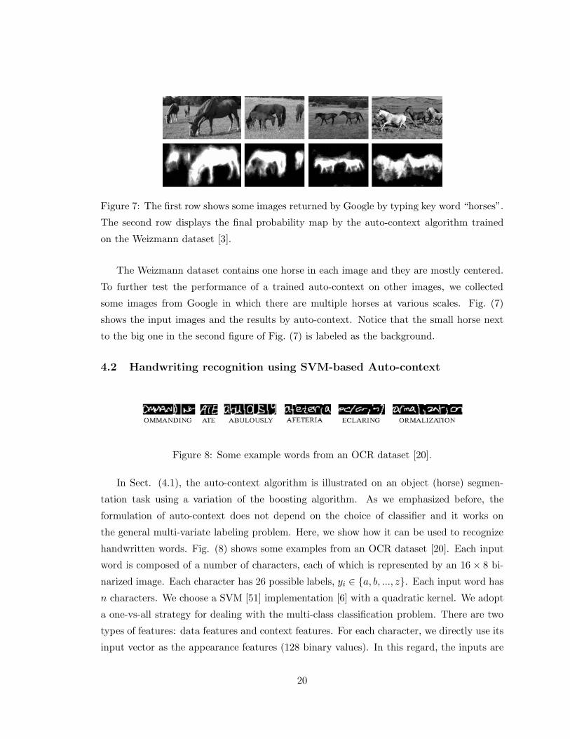
Figure 7: The first row shows some images returned by Google by typing key word “horses”.

The second row displays the final probability map by the auto-context algorithm trained

on the Weizmann dataset [3].

The Weizmann dataset contains one horse in each image and they are mostly centered.

To further test the performance of a trained auto-context on other images, we collected

some images from Google in which there are multiple horses at various scales. Fig. (7)

shows the input images and the results by auto-context. Notice that the small horse next

to the big one in the second figure of Fig. (7) is labeled as the background.

4.2 Handwriting recognition using SVM-based Auto-context

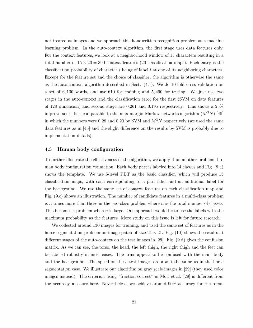
Figure 8: Some example words from an OCR dataset [20].

In Sect. (4.1), the auto-context algorithm is illustrated on an object (horse) segmen-

tation task using a variation of the boosting algorithm. As we emphasized before, the

formulation of auto-context does not depend on the choice of classifier and it works on

the general multi-variate labeling problem. Here, we show how it can be used to recognize

handwritten words. Fig. (8) shows some examples from an OCR dataset [20]. Each input

word is composed of a number of characters, each of which is represented by an 16 × 8 bi-

narized image. Each character has 26 possible labels, yi ∈ {a, b, ..., z}. Each input word has

n characters. We choose a SVM [51] implementation [6] with a quadratic kernel. We adopt

a one-vs-all strategy for dealing with the multi-class classification problem. There are two

types of features: data features and context features. For each character, we directly use its

input vector as the appearance features (128 binary values). In this regard, the inputs are

20

not treated as images and we approach this handwritten recognition problem as a machine

learning problem. In the auto-context algorithm, the first stage uses data features only.

For the context features, we look at a neighborhood window of 15 characters resulting in a

total number of 15 × 26 = 390 context features (26 classification maps). Each entry is the

classification probability of character i being of label l at one of its neighboring characters.

Except for the feature set and the choice of classifier, the algorithm is otherwise the same

as the auto-context algorithm described in Sect. (4.1). We do 10-fold cross validation on

a set of 6, 100 words, and use 610 for training and 5, 490 for testing. We just use two

stages in the auto-context and the classification error for the first (SVM on data features

of 128 dimension) and second stage are 0.261 and 0.195 respectively. This shows a 25%

improvement. It is comparable to the max-margin Markov networks algorithm (M3N) [45]

in which the numbers were 0.28 and 0.20 by SVM and M3N respectively (we used the same

data features as in [45] and the slight difference on the results by SVM is probably due to

implementation details).

4.3 Human body configuration

To further illustrate the effectiveness of the algorithm, we apply it on another problem, hu-

man body configuration estimation. Each body part is labeled into 14 classes and Fig. (9.a)

shows the template. We use 5-level PBT as the basic classifier, which will produce 15

classification maps, with each corresponding to a part label and an additional label for

the background. We use the same set of context features on each classification map and

Fig. (9.c) shows an illustration. The number of candidate features in a multi-class problem

is n times more than those in the two-class problem where n is the total number of classes.

This becomes a problem when n is large. One approach would be to use the labels with the

maximum probability as the features. More study on this issue is left for future research.

We collected around 130 images for training, and used the same set of features as in the

horse segmentation problem on image patch of size 21× 21. Fig. (10) shows the results at

different stages of the auto-context on the test images in [29]. Fig. (9.d) gives the confusion

matrix. As we can see, the torso, the head, the left thigh, the right thigh and the feet can

be labeled robustly in most cases. The arms appear to be confused with the main body

and the background. The speed on these test images are about the same as in the horse

segmentation case. We illustrate our algorithm on gray scale images in [29] (they used color

images instead). The criterion using “fraction correct” in Mori et al. [29] is different from

the accuracy measure here. Nevertheless, we achieve around 90% accuracy for the torso,

21

(a) template (b) input (c) context features (d) confusion matrix

Figure 9: (a) Shows a template in which body parts are colored into 14 labels. (b) Is a test

image and (c) Illustrates context features on the discriminative probability maps with each

corresponding to a class label. (d) Shows the confusion matrix for the test images.

which is comparable to the 91% fraction correct rate reported in [29]. Further procedures

are still required to explicitly extract the body parts since the auto-context algorithm only

outputs probability maps. This is probably the place where more explicit shape information

can be used in the Bayesian framework.

4.4 Scene parsing/labeling

We also applied our algorithm on the task of scene parsing/region labeling. We used the

MSRC dataset [41] of 591 images with 21 types of objects manually segmented and labeled

(there are two additional types in the new dataset). There is a nuisance category labeled

as 0. The setting for this task is similar as before, and the only difference is that we use

color images in this case. Shotton et al. did not have the background model to learn the

regions of 0 label, whereas it is not a problem in our case. However, to obtain a direct

comparison to their result, we also exclude the 0 label both in training and testing. We use

the identical training and testing images as in [41]. Fig. (11) shows some results and the

confusion matrix. The results by auto-context are the marginal probabilities for each pixel

belonging to a specific class. We simply assign the label with the highest probability to each

pixel. Note that Shotton [41] did not model the 0 class. There are two additional classes,

“horse” and “mountain” which were not included in [41]. The accuracy by the first stage

of auto-context, classification method PBT only, achieves 50.4%. The overall pixel-wise

accuracy by 4 stages of auto-context is 74.5% which is better than 72.2% reported in [41].

Starting from the second stage of the auto-context algorithm, spatial relationships of the

22

Figure 10: The first row displays some test images. The second, third and forth row

shows the classification maps by the first, third and fifth stage of the trained auto-context

algorithm.

labels (both same and different) at different locations are fused implicitly through classifiers.

For example, a pixel classified as being a confusing pattern between boat and building will

be clarified as boat, if some context pixels (top, bottom, left and right) in a range have

high probability of being water. In this regard, contextual relationships are maintained in

auto-context in an implicit way through individual pixels. To understand how the context

features are explicitly playing the role in the algorithm, we give a description of some

selected features in the second stage of the algorithm. For a multi-class labeling problem,

after each round, n discriminative probability (classification) maps p, corresponding to each

class label, are created. In the learning process (after the first stage), the algorithm can

choose both appearance and context features to support the decision making. Usually, the

first three features selected are still from each class’s own probability map. The second

column in Table (1) gives a description to the fourth features for some typical classes. Each

class picks the mean value of a small window surrounding or near the current pixel. The

third column of Table (1) describes the forth selected feature. Clearly, context information

are being selected and it can be understood intuitively. For example, a pixel on a face

looks for context support from body, and a boat pixel looks somewhere up-right for water.

Sometimes, appearance features are still selected for some classes, e.g. the tree class.

23

Bu Gs Tr Co Sp Sk Ap W Fc Ca Bi Fl Sn Bi Bk Ch Rd Ct Dg Bd Bt Building 69 1 5 0 0 1 1 3 1 1 2 2 1 1 5 0 4 1 0 2 0

Grass 0 96 1 1 1 0 0 1 0 0 0 0 0 0 0 0 0 0 0 0 0

Tree 3 5 87 0 0 1 0 1 0 0 1 1 0 0 0 0 0 0 0 0 0

Cow 0 5 1 78 1 0 0 0 1 0 0 0 1 0 0 0 0 1 5 7 0 Sheep 1 5 3 3 80 0 0 0 0 0 0 0 0 2 0 3 2 0 0 0 0 Sky 3 0 0 0 0 95 0 1 0 0 0 0 0 0 0 0 0 0 0 0 0 Airplane 11 2 2 0 0 1 83 0 0 0 0 0 0 0 0 0 0 0 0 0 0 Water 5 5 2 0 0 2 0 67 0 3 3 0 0 1 0 0 9 0 0 1 2 Face 1 0 0 1 0 0 0 0 84 0 0 0 0 0 1 0 0 0 1 10 0 Car 14 0 1 0 0 2 3 1 0 70 0 0 1 1 1 0 4 0 0 1 2 Bike 12 0 2 0 0 0 0 1 0 1 79 0 0 0 0 0 2 0 0 2 0 Flower 1 1 2 7 2 0 0 1 3 0 0 47 0 3 17 0 0 1 1 12 0 Sign 34 0 1 0 0 0 0 0 0 0 0 0 61 0 2 0 1 1 0 0 0 Bird 9 7 3 5 10 3 0 13 1 6 0 0 0 30 0 1 2 2 6 1 0 Book 8 1 1 0 0 0 0 0 1 0 0 3 0 0 80 2 1 0 0 2 0 Chair 25 2 8 1 0 0 0 1 3 0 4 2 0 0 4 45 1 1 0 2 0 Road 11 0 1 0 0 1 0 6 0 1 0 0 0 0 0 0 78 0 0 1 0 Cat 1 0 4 0 0 0 0 11 2 0 0 0 0 4 0 1 3 68 5 0 0 Dog 4 2 5 4 3 0 0 2 7 0 0 0 0 9 0 1 3 5 52 2 0 Body 6 1 1 2 0 0 0 1 5 0 0 1 1 2 5 1 2 3 2 67 0 Boat 28 0 0 0 0 1 3 15 0 13 9 0 0 1 0 0 2 0 0 2 27

Figure 11: The first row shows some difficult test images and a few typical ones, with their

corresponding classified labels. The second row displays the legend and confusion matrix.

The overall pixel-wise accuracy is 74.5%. The result by image patch-based classification

achieves 50.4%. The number reported in [41] was 72.2%, and using auto-context with a

post-processing stage achieves 77.7%.

The final probability maps observe certain degree of “noisiness” since no explicit con-

straints were used in the classification stage. Therefore, enforcing smoothness and region-

based consistency can further improve the results. Here, we simply employ a post-processing

process to encourage the neighboring pixels to have the same label as in eqn. (8).

Y ∗ = argmin−∑

i

log p(yi|X) + α∑(i,j)

δ(yi �= yj), (8)

where α = 2.0 for the results in this paper. Eqn. (8) essentially combines the classifica-

tion map by auto-context with a Potts model. Based on the probability maps output by

the auto-context algorithm, we simply perform a Iterated Conditional Modes (ICM) [28]

method to perform energy minimization, which requires 0.1 seconds. Qualitatively, the seg-

mentation/labeling results did not change too much. Quantitatively, the accuracy improves

24

to 77.7%, which is probably due to the sensitiveness of the accuracy measure on the object

boundaries. Ideally, smoothness between the neighboring pixels can also be captured by

the context features and this post-processing seems to be redundant. However, the auto-

context algorithm fuses many other context features and thus, the consistency is maintained

implicitly. Eqn. (8), on the other hand, maintains the local smoothness explicitly (in [19]

we can see that this post-processing can be removed by a voting-based scheme).

The recognition rate averaged over all the classes is 68.7% whereas it was reported

as 64% and 67% in [52] and [40] respectively. Also, a careful reading at the confusion

matrices by both the algorithms shows that our result is more consistent and the mistakes

made are more “reasonable”. For example, boat is mostly confused with car and building

whereas boat was mis-classified to many other classes in [41] such as water, bike, and tree.

Our algorithm is more general and easier to implement. The speed reported in [41] was 3

minutes per image whereas ours is around 70 seconds. A significantly improved algorithm

in speed has been proposed in [40] with nearly real-time performance. However, the average

accuracy is 72%.

It is noted that almost all the algorithms we compared to, on the horse segmentation,

human body configuration, and scene labeling, use context or high-level information. CRF

models are indeed context-based. A direct comparison to the algorithms reported on the

MSRC dataset is given in table (2). [35] Gave the accuracy measure on segmented regions

rather than pixels with a score 68.4%.

Algorithm TextonBoost [41] [57] Auto-Context AC+post

Accuracy 72.2% 75.1% 74.5% 77.7%

Table 2: Comparison to other algorithms on the MSRC dataset. AC+post refers to the

result by auto-context with a post-processing for smoothing (which takes about .1 seconds

per image).

4.5 Single structure segmentation in 3D brain images

As previously stated, context information plays an important role in medical image analysis

where the anatomical structures are roughly positioned and constrained. Segmenting sub-

cortical structures from 3D brain images is of significant practical importance.

We first show our algorithm on a recently established caudate segmentation dataset [50].

There are 4 sets of data provided in this grand challenge competition, 2 for training and

25

hybrid model

auto-context model

Figure 12: The first row displays the results by the Hybrid model [49] and the second row

shows the results on the same slices by the auto-context algorithm. The red lines are the

boundaries by the neuroanatomists and blue lines are the boundaries by the algorithm.

2 for testing. As described in the documents from the organizers: “All MRI images are

scanned with an Inversion Recovery Prepped Spoiled Grass sequence on a variety of scan-

ners (GE, Siemens, Philips, mostly 1.5 Tesla). Some datasets have been acquired in axial

direction, whereas others in coronal direction. All datasets have been re-oriented to axial

RAI-orientation, but have not been aligned in any fashion.” The 2 training sets are: (1)

MRIs and structural segmentations from the internet brain segmentation repository (IBSR)

at Mass General Hospital, Boston. (2) MRIs and caudate segmentations from the Psychia-

try Neuroimaging Laboratory at the Brigham and Women’s Hospital Boston (BWH). The

2 testing sets are: (1) MRIs from different disease study at the UNC Neuro Image Analysis

Laboratory, Chapel Hill. (2) 14 MRIs from the Psychiatry Neuroimaging Laboratory at

the Brigham and Womens Hospital, Boston. This data is from the same study as the BWH

datasets in the training set.

The training sets BWH and IBSR are given as different forms. We use a popular

tool, BET [43], to perform automatic skull stripping, followed by a widely used 3D image

registration algorithm, AIR [55], to perform 12-parameter non-rigid transformation. A

typical image in the IBSR training image is used as the template. Based on these 25

training images with the left and right caudate manually delineated by experts, we train

auto-context to learn 6 stages of classifiers. Since the images are roughly registered, position

26

Case OE Score VD Score AD Score RMSD Score MD Score Total

UNC Ped 40.4 74.6 -23.2 59.5 0.86 68.3 1.21 78.4 5.64 83.4 72.82

UNC Eld 38.8 75.6 -17.2 69.8 0.75 72.2 1.14 79.6 6.79 80.0 75.44

BWH PNL 41.8 73.7 -26.6 53.8 1.51 49.1 3.50 42.1 25.27 28.4 49.42

Average All 40.8 74.3 -23.9 58.3 1.22 57.9 2.53 57.5 17.33 50.6 59.71

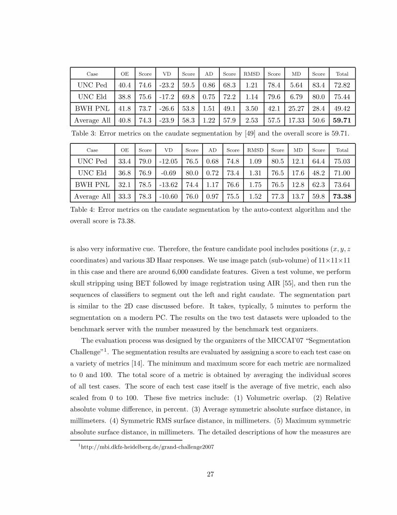
Table 3: Error metrics on the caudate segmentation by [49] and the overall score is 59.71.

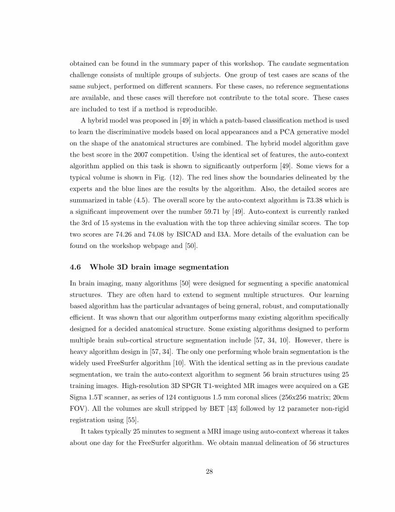
Case OE Score VD Score AD Score RMSD Score MD Score Total

UNC Ped 33.4 79.0 -12.05 76.5 0.68 74.8 1.09 80.5 12.1 64.4 75.03

UNC Eld 36.8 76.9 -0.69 80.0 0.72 73.4 1.31 76.5 17.6 48.2 71.00

BWH PNL 32.1 78.5 -13.62 74.4 1.17 76.6 1.75 76.5 12.8 62.3 73.64

Average All 33.3 78.3 -10.60 76.0 0.97 75.5 1.52 77.3 13.7 59.8 73.38

Table 4: Error metrics on the caudate segmentation by the auto-context algorithm and the

overall score is 73.38.

is also very informative cue. Therefore, the feature candidate pool includes positions (x, y, z

coordinates) and various 3D Haar responses. We use image patch (sub-volume) of 11×11×11

in this case and there are around 6,000 candidate features. Given a test volume, we perform

skull stripping using BET followed by image registration using AIR [55], and then run the

sequences of classifiers to segment out the left and right caudate. The segmentation part

is similar to the 2D case discussed before. It takes, typically, 5 minutes to perform the

segmentation on a modern PC. The results on the two test datasets were uploaded to the

benchmark server with the number measured by the benchmark test organizers.

The evaluation process was designed by the organizers of the MICCAI’07 “Segmentation

Challenge”1. The segmentation results are evaluated by assigning a score to each test case on

a variety of metrics [14]. The minimum and maximum score for each metric are normalized

to 0 and 100. The total score of a metric is obtained by averaging the individual scores

of all test cases. The score of each test case itself is the average of five metric, each also

scaled from 0 to 100. These five metrics include: (1) Volumetric overlap. (2) Relative

absolute volume difference, in percent. (3) Average symmetric absolute surface distance, in

millimeters. (4) Symmetric RMS surface distance, in millimeters. (5) Maximum symmetric

absolute surface distance, in millimeters. The detailed descriptions of how the measures are

1http://mbi.dkfz-heidelberg.de/grand-challenge2007

27

obtained can be found in the summary paper of this workshop. The caudate segmentation

challenge consists of multiple groups of subjects. One group of test cases are scans of the

same subject, performed on different scanners. For these cases, no reference segmentations

are available, and these cases will therefore not contribute to the total score. These cases

are included to test if a method is reproducible.

A hybrid model was proposed in [49] in which a patch-based classification method is used

to learn the discriminative models based on local appearances and a PCA generative model

on the shape of the anatomical structures are combined. The hybrid model algorithm gave

the best score in the 2007 competition. Using the identical set of features, the auto-context

algorithm applied on this task is shown to significantly outperform [49]. Some views for a

typical volume is shown in Fig. (12). The red lines show the boundaries delineated by the

experts and the blue lines are the results by the algorithm. Also, the detailed scores are

summarized in table (4.5). The overall score by the auto-context algorithm is 73.38 which is

a significant improvement over the number 59.71 by [49]. Auto-context is currently ranked

the 3rd of 15 systems in the evaluation with the top three achieving similar scores. The top

two scores are 74.26 and 74.08 by ISICAD and I3A. More details of the evaluation can be

found on the workshop webpage and [50].

4.6 Whole 3D brain image segmentation

In brain imaging, many algorithms [50] were designed for segmenting a specific anatomical

structures. They are often hard to extend to segment multiple structures. Our learning

based algorithm has the particular advantages of being general, robust, and computationally

efficient. It was shown that our algorithm outperforms many existing algorithm specifically

designed for a decided anatomical structure. Some existing algorithms designed to perform

multiple brain sub-cortical structure segmentation include [57, 34, 10]. However, there is

heavy algorithm design in [57, 34]. The only one performing whole brain segmentation is the

widely used FreeSurfer algorithm [10]. With the identical setting as in the previous caudate

segmentation, we train the auto-context algorithm to segment 56 brain structures using 25

training images. High-resolution 3D SPGR T1-weighted MR images were acquired on a GE

Signa 1.5T scanner, as series of 124 contiguous 1.5 mm coronal slices (256x256 matrix; 20cm

FOV). All the volumes are skull stripped by BET [43] followed by 12 parameter non-rigid

registration using [55].

It takes typically 25 minutes to segment a MRI image using auto-context whereas it takes

about one day for the FreeSurfer algorithm. We obtain manual delineation of 56 structures

28

by neuroanatomists, such as caudate, hippocampus, putamen, cerebellum, insular cortex,

gyrus rectus. An example test volume is shown in Fig. (13) in which the first row shows

the manual delineation, the second row shows the result by the first stage of patch-based

classifier, and the third row shows the result by the final stage. We use 15 test volumes and

repeat the training and testing images a couple of times. It was shown in [49] that FreeSurfer

produces a worse result than using the learning-based hybrid algorithm. The average F-

value for all 56 anatomical structures is 78.0% which improves the hybrid algorithm with

score 75.8%.

manual

step 1

step 3

Figure 13: The first row displays a typical test images with 56 structures annotated by

neuroanatomists. The second and third row show the results by the first and third stage of

the auto-context algorithm respectively.

5 Conclusions and discussions

In this paper, we have introduced the auto-context algorithm, which learns the low-level

appearance, implicit shape, and context information through a sequence of discriminative

29

models. Our goal is to design an integrated framework to include both appearance and

context information in a principled way. We target the posterior distribution directly, and

thus, the test phase shares the same procedures as those in the training. The auto-context

algorithm selects and fuses a large number of supporting contexts, which allow it to rapidly

propagate the information. We introduce iterative procedures into traditional classification

algorithms to refine the classification results by using context information effectively.

The proposed algorithm is very general. We illustrate the auto-context algorithm on

three challenging vision tasks. The results are shown to significantly improve the results by

patch-based classification algorithms and demonstrate improved results over many existing

algorithms using CRFs and MRFs. It typically takes about 30 ∼ 70 seconds to run the

algorithm on an image of size around 300 × 200. We also demonstrated the auto-context

algorithm on two important brain imaging tasks and showed significantly improved results

over state-of-the-art algorithms. Moreover, the scope of the auto-context model goes beyond

vision applications and it can be applied in other problems of multi-variate labeling in

machine learning and AI.

In terms of the advantages, the auto-context algorithm greatly improves the modeling

capability of existing methods based on MRFs and CRFs. It does not depend on any par-

ticular type of classifier, is very general and easy to implement, and avoids heavy algorithm

design (various energy terms and procedures). In terms of the disadvantages, shape and

context information in auto-context are utilized in an implicit way. There is a certain limit

this type of implicit information can go through discriminative learning. More explicit

shape information and object configuration obtained through top-down reasoning, e.g. the

silhouette of a shape, can further clarify certain ambiguities, though a more time-consuming

inference step may be required. The other limitations for the auto-context model are: (1)

the features on the context information are still somewhat limited; (2) different auto-context

models need to be trained for different applications; (3) the algorithm is a supervised method

and thus requires a set of well-annotated ground truth data, which might not always be

available or can be difficult to obtain. We are also exploring using weakly-supervised and

semi-supervised learning to alleviate the burden on obtaining ground truth data.

6 Acknowledgment

This work is supported by Office of Naval Research Award, No. N000140910099. Any

findings, and conclusions or recommendations expressed in this material are those of the

authors and do not necessarily reflect the views of the Office of Naval Research. This work

30

is also in part funded by NSF No. 0844566 and NIH Grant U54 RR021813 entitled Center

for Computational Biology. We thank Yingnian Wu and Piotr Dollar for many stimulat-

ing discussions. We also thank the anonymous reviewers for providing many constructive

suggestions.

References

[1] S. Avidan. Spatialboost: Adding spatial reasoning to adaboost. In Proc. of ECCV,

2006.

[2] S. Belongie, J. Malik, and J. Puzicha. Shape matching and object recognition using

shape contexts. IEEE Trans. on PAMI, 24(4):509–522, April 2002.

[3] E. Borenstein, E. Sharon, and S. Ullman. Combining top-down and bottom-up seg-

mentation. In Proc. IEEE workshop on Perc. Org. in Com. Vis., June 2004.

[4] L. Breiman, J. H. Friedman, R. A. Olshen, and C. J. Stone. Classification and regression

trees. Wadsworth International, Belmont, Ca, 1984.

[5] R. Caruana and A. Niculescu-Mizil. An empirical comparison of supervised learning

algorithms. In Proc. of ICML, 2006.

[6] C. C. Chang and C. J. Lin. LIBSVM: a library for support vector machines, 2001.

Software available at http://www.csie.ntu.edu.tw/ cjlin/libsvm.

[7] N. Dalal and B. Triggs. Histograms of oriented gradients for human detection. In Proc.

of CVPR, June 2005.

[8] T. G. Dietterich and G. Bakiri. Solving multiclass learning problems via error-

correcting output codes. J. of Art. Intelligence Res., 2:263–286, 1995.

[9] M. Fink and P. Perona. Mutual boosting for contextual inference. In Proc. of NIPS,

2003.

[10] B. Fischl, D. Salat, E. Busa, M. Albert, M. Dieterich, C. Haselgrove, A. van der Kouwe,

R. Killiany, S. K. D. Kennedy, A. Montillo, N. Makris, B. Rosen, and A. Dale. Whole

brain segmentation: automated labeling of neuroanatomical structures in the human

brain. Neuron, 33:341–355, 2002.

[11] Y. Freund and R. E. Schapire. A decision-theoretic generalization of on-line learning

and an application to boosting. J. of Comp. and Sys. Sci., 55(1):119–139, 1997.

[12] J. Friedman, T. Hastie, and R. Tibshirani. Additive logistic regression: a statistical

view of boosting. Dept. of Statistics, Stanford Univ. Technical Report., 1998.

31

[13] S. Geman and D. Geman. Gibbs distributions, and the bayesian restoration of images.

IEEE Trans. PAMI, 6:721–741, Nov. 1984.

[14] G. Gerig, M. Chakos, and M. Valmet. A new validation tool for assessing and improving

3d object segmentation. In Proc of MICCAI, pages 516–523, 2001.

[15] X. He, R. Zemel, and M. Carreira-Perpinan. Multiscale conditional random fields for

image labelling. In Proc. of CVPR, June 2004.

[16] D. Hoiem, A. Efros, and M. Hebert. Geometric context from a single image. In Proc.

of CVPR, June 2005.

[17] D. Hoiem, A. Efros, and M. Hebert. Closing the loop on scene interpretation. In Proc.

of CVPR, June 2008.

[18] D. Hoiem, A. Efros, and M. Hebert. Putting objects in perspective. Int’l J. of Comp.

Vis, (1), Oc. 2008.

[19] J. Jiang and Z. Tu. Efficient scale space auto-context for image segmentation and

labeling. In Proc. of CVPR, 2009.

[20] R. Kassel. A Comparison of Approaches to On-line Handwritten Character Recognition.

PhD thesis, MIT Spoken Language Systems Group, 1995.

[21] S. Kumar and M. Hebert. Discriminative random fields: a discriminative framework

for contextual interaction in classification. In Proc. of ICCV, Oct. 2003.

[22] S. Kumar and M. Hebert. A hierarchical field framework for unified context-based

classification. In Proc. of ICCV, Oct. 2005.

[23] J. Lafferty, A. McCallum, and F. Pereira. Conditional random fields: probabilistic

models for segmenting and labeling sequence data. In Proc. of 10th Int’l Conf. on

Machine Learning, pages 282–289, San Francisco, 2001.

[24] Z. Lao, D. Shen, A. Jawad, B. Karacali, D. Liu, E. Melhem, N. Bryan, and C. Da-

vatzikos. Automated segmentation of white matter lesions in 3d brain mr images,

using multivariate pattern classification. In Proc. of 3rd IEEE In’l Symp. on Biomed-

ical Imaging (ISBI), April 2006.

[25] Y. LeCun, F. Huang, and L. Bottou. Learning methods for generic object recognition

with invariance to pose and lighting. In Proc. of CVPR, June 2004.

[26] C. Li, D. B. Goldgof, and L. O. Hall. Knowledge-based classification and tissue labeling

of mr images of human brain. IEEE Trans. on Medical Imaging, 12(4):740–750, Dec.

1993.

32

[27] C. B. Liu, A. Toga, and Z. Tu. Fusing adaptive atlas and informative features for robust

3d brain image segmentation. In Technical Report, Lab of Neuro Imaging, UCLA, 2009.

[28] J. Liu. Monte Carlo Strategies in Scientific Computing. Springer-Verlag NY INC, 2001.

[29] G. Mori, X. Ren, A. Efros, and J. Malik. Recovering human body configurations:

Combining segmentation and recognition. In Proc. of CVPR, June 2004.

[30] K. L. Narr, P. M. Thompson, T. Sharma, J. Moussai, R. Blanton, B. Anvar, A. Edris,

R. Krupp, J. Rayman, M. Khaledy, and A. W. Toga. Three-dimensional mapping of

temporo-limbic regions and the lateral ventricles in schizophrenia: gender effects. Biol

Psychiatry, 50(2):84–97, 2001.

[31] A. Oliva and A. Torralba. The role of context in object recognition. Trends in Cognitive

Sciences, 11(12):520–527, Dec. 2007.

[32] J. Pearl. Probabilistic reasoning in intelligent systems: networks of plausible inference.

Morgan Kaufmann, 1988.

[33] S. Pizer, T. Fletcher, Y. Fridman, D. Fritsch, A. Gash, J. Glotzer, S. Joshi, A. Thall,

G. Tracton, P. Yushkevich, and E. Chaney. Deformable m-reps for 3d medical image

segmentation. Int’l. J. of Comp. Vis., 55(2):85–106, 2003.

[34] K. Pohl, J. Fisher, R. Kikinis, W. Grimson, and W. Wells. A bayesian model for joint

segmentation and registration. NeuroImage, 31(1):228–239, 2006.

[35] A. Rabinovich, A. Vedaldi, C. Galleguillos, E. Wiewiora, and S. Belongie. Objects in

context. In Proc. of ICCV, Oct. 2007.

[36] X. Ren, C. Fowlkes, and J. Malik. Cue integration in figure/ground labeling. In Proc.

of NIPS, 2005.

[37] R. Rifkin and A. Klautau. In defence of one-vs-all classification. J. Mach. Learn. Res.,

5:101–141, 2004.

[38] T. Rohlfing, D. B. Russakoff, and J. C. R. Maurer. Performance-based classifier com-

bination in atlas-based image segmentation using expectation-maximization parameter

estimation. IEEE Trans. on Medical Imaging, 23(8):983–994, August 2004.

[39] R. E. Schapire, R. E. Freund, P. Bartlett, and W. S. Lee. Boosting the margin: A

new explanation for the effectiveness of voting methods. The Annals of Statistics,

26:1651–1686, 1998.

[40] J. Shotton, M. Johnson, and R. Cipolla. Semantic texton forests for image categoriza-

tion and segmentation. In Proc. of CVPR, 2008.

33

[41] J. Shotton, J. Winn, C. Rother, and A. Criminisi. Textonboost: Joint appearance,

shape and context modeling for mult-class object recognition and segmentation. In

Proc. of ECCV, 2006.

[42] A. Singhal, J. Luo, and W. Zhu. Probabilistic spatial context models for scene content

understanding. In Proc. of CVPR, June 2003.

[43] S. Smith. Fast robust automated brain extraction. Hum Brain Mapp, 17(3):856–76,

2001.

[44] R. Szeliski, R. Zabih, D. Scharstein, O. Veksler, V. Kolmogorov, A. Agarwala, M. Tap-

pen, and C. Rother. A comparative study of energy minimization methods for markov

random fields. In Proc. of ECCV, 2006.

[45] B. Taskar, C. Guestrin, and D. Koller. Max-margin markov networks. In NIPS, 2003.

[46] A. Torralba, K. P. Murphy, and W. T. Freeman. Contextual models for object detection

using boosted random fields. In Proc. of NIPS, 2004.

[47] Z. Tu. Probabilistic boosting tree: Learning discriminative models for classification,

recognition, and clustering. In Proc. of Int’l Conf. on Comp. Vis. (ICCV), pages

1589–1596, Beijing, Oct. 2005.

[48] Z. Tu, X. Chen, A. Yuille, and S. Zhu. Image parsing: unifying segmentation, detection,

and object recognition. Int’l J. of Com. Vis., 63(2):113–140, July 2005.

[49] Z. Tu, K. Narr, P. Dollar, P. Thompson, and A. Toga. Brain anatomical structure pars-

ing by hybrid discriminative/generative models. IEEE Tran. Med. Imaging, 27(4):495–

508, April 2008.

[50] B. van Ginneken, T. Heimann, and M. Styner. 3D Segmentation in the Clinic: A

Grand Challenge. Proc. of MICCAI Workshop, 2007.

[51] V. Vapnik. Estimation of dependences based on empirical data. Springer-Verlag, 1982.

[52] J. Verbeek and B. Triggs. Region classification with markov field aspect models. In

Proc. of CVPR, June 2007.

[53] P. A. Viola and M. J. Jones. Robust real-time face detection. Int’l J. of Comp. Vis.,

57(2):137–154, 2004.

[54] L. Wolf and S. Bileschi. A critical view of context. Int’l J. on Com. Vis., 2006.

[55] R. P. Woods, J. C. Mazziotta, and S. R. Cherry. Mri-pet registration with automated

algorithm. Journal of Computer Assisted Tomography, 17:536–546, 1993.

[56] Y. Wu and J. Fan. Contextual flow. In Proc. of CVPR, 2009.

34

[57] J. Yang, L. H. Staib, and J. S. Duncan. Neighbor-constrained segmentation with level

set based 3d deformable models. IEEE Trans. on Medical Imaging, 23(8):940–948,

Aug. 2004.

[58] M. Yang, G. Hua, and Y. Wu. Context-aware visual tracking. IEEE Trans. Pattern

Anal. Mach. Intell., 31(7):1195–1209, 2009.

[59] J. Yedidia, W. Freeman, and Y. Weiss. Generalized belief propagation. In Proc. of

NIPS, 2000.

35