author's personal copy -...
TRANSCRIPT

Influence of experimental extreme water pulseson greenhouse gas emissions from soils
Sandra Petrakis . Angelia Seyfferth . Jinjun Kan .
Shreeram Inamdar . Rodrigo Vargas
Received: 1 June 2016 / Accepted: 4 March 2017
� Springer International Publishing Switzerland 2017
Abstract Climate models predict increased fre-
quency and intensity of storm events, but it is unclear
how extreme precipitation events influence the
dynamics of soil fluxes for multiple greenhouse gases
(GHGs). Intact soil mesocosms (0–10 cm depth) from
a temperate forested watershed in the piedmont region
of Maryland [two upland forest soils, and two hydric
soils (i.e., wetland, creek bank)] were exposed to
experimental water pulses with periods of drying,
forcing soils towards extreme wet conditions under
controlled temperature. Automated measurements
(hourly resolution) of soil CO2, CH4, and N2O fluxes
were coupled with porewater chemistry analyses (i.e.,
pH, Eh, Fe, S, NO3-), and polymerase chain reaction–
denaturing gradient gel electrophoresis to characterize
changes in microbial community structure. Automated
measurements quantified unexpected increases in
emissions up to 245% for CO2 (Wetland),[23,000%
for CH4 (Creek), and [110,000% for N2O (Forest
Soils) following pulse events. The Creek soil produced
the highest soil CO2 emissions, the Wetland soil
produced the highest CH4 emissions, and the Forest
soils produced the highest N2O emissions during the
experiment. Using carbon dioxide equivalencies of the
three GHGs, we determined the Creek soil contributed
the most to a 20-year global warming potential (GWP;
30.3%). Forest soils contributed the most to the
100-year GWP (up to 53.7%) as a result of large
N2O emissions. These results provide insights on the
influence of extreme wet conditions on porewater
chemistry and factors controlling soil GHGs fluxes.
Finally, this study addresses the need to test biogeo-
chemical thresholds and responses of ecosystem
functions to climate extremes.
Keywords Carbon dioxide � Continuousmeasurements � Extreme events � Methane � Nitrousoxide
Introduction
Carbon dioxide (CO2), methane (CH4), and nitrous
oxide (N2O) are greenhouse gases (GHGs) that
contribute to global warming and feedbacks to climate
change (Stocker et al. 2013). One consequence of
shifting precipitation regimes as a result of global
environmental change is the increased frequency and
Responsible Editor: Asmeret Asefaw Berhe.
Electronic supplementary material The online version ofthis article (doi:10.1007/s10533-017-0320-2) contains supple-mentary material, which is available to authorized users.
S. Petrakis � A. Seyfferth � S. Inamdar � R. Vargas (&)
Department of Plant and Soil Sciences, University of
Delaware, Newark, DE 19716, USA
e-mail: [email protected]
J. Kan
Stroud Water Research Center, 970 Spencer Road,
Avondale, PA 19311, USA
123
Biogeochemistry
DOI 10.1007/s10533-017-0320-2
Author's personal copy

intensity of large, powerful tropical cyclones (IPCC,
2014). As such, it is critical to understand how extreme
events such as hurricanes influence ecosystem pro-
cesses such as lateral transport of organic matter
(Dhillon and Inamdar 2013) and vertical GHG fluxes
(Vargas 2012) around the globe. The production of
these GHGs, and the potential for soils to behave as
sinks or sources of these GHGs, is directly influenced
by nutrient availability (Erickson and Perakis 2014),
redox potential (Eh) (Dalal et al. 2008; Hall et al.
2013), temperature, and soil moisture (Davidson et al.
1998; Borken and Matzner 2009). Heavy rewetting of
soils promotes reducing conditions, alters the avail-
ability of dissolved solutes and rates of C mineraliza-
tion, and lowers gas diffusivity in soils (Fierer and
Schimel 2002; McNicol and Silver 2014; Vargas
2012). Therefore, it is important to understand the
many processes involved in the production and release
of GHGs from soils following rapid changes in soil
moisture (Kim et al. 2012).
Recent attention has been directed towards the
influence of extreme weather events on ecosystem
processes (Kim et al. 2012; Sutherland et al. 2013;
Frank et al. 2015). By definition, extreme weather
events are rare, and therefore few direct measurements
of ecosystem responses to these events exist. This
limits our capacity to understand and develop prog-
nostic capabilities for the responses of ecosystem
processes. Extreme precipitation events rapidly
increase soil water content, can impact the microbial
community structure (Knapp et al. 2008), and alter
dynamics of GHG production in soils, with CO2 being
themost studied andwell understood (Kim et al. 2012).
Following rewetting, soil gas fluxes can increase by up
to 9000% for CO2, 9790% for N2O, and there are
smaller but uncertain responses for CH4 (Kim et al.
2012). Many studies address the addition of water to
soils with either drought-stressed or dry antecedent
conditions (Fierer and Schimel 2002; Smith et al. 2003;
Muhr et al. 2008; Borken and Matzner 2009). Addi-
tionally, soil moisture may be limiting to mineraliza-
tion of C and N after a wetting event, increasing the
flush of C and N in response to water additions to dry
soils known as the ‘Birch effect’ (Jarvis et al. 2007);
very high levers of soilmoisturemay also be limiting to
C and N mineralization (Lado-Monserrat et al. 2014).
It is known that wetting of dry soils can increase
microbial activity within minutes or hours, as soil
organic matter is mineralized (Borken and Matzner
2009), and anaerobic conditions and decreased diffu-
sivity may explain decreases in CO2 fluxes under very
wet conditions (Kim et al. 2012; Hall et al. 2013).
Although one of the most studied terrestrial ecosys-
tem processes is the production of CO2 in soils
(Schlesinger and Andrews 2000), few studies have
simultaneously measured CO2, CH4, and N2O fluxes
from soils with moist or very wet antecedent condi-
tions (McNicol and Silver 2014). As such, more
comprehensive understanding of the rapid responses of
soils under different moisture conditions for multiple
GHGs (i.e., CO2, CH4, and N2O) is warranted. As a
result of the cost of instrumentation and availability of
current technology, most studies have focused on
manual measurements of CO2 efflux, but few have
reported continuous measurements of CO2, N2O and
CH4 (Savage et al. 2014). Research suggests that that
the magnitude of GHG fluxes are dependent upon
spatial heterogeneity and topographic location (Pacific
et al. 2009; Riveros-Iregui and McGlynn 2009; Leon
et al. 2014), and that a tradeoff exists between temporal
and spatial sampling techniques (Savage andDavidson
2003). Recent technological advances on automated
measurement systems can provide the high temporal
resolution needed for tracking rapid changes in soil
GHG emissions and responses to water pulses (Vargas
et al. 2011; Savage et al. 2014). Furthermore, time
series analysis of high temporal frequency measure-
ments could discern the timescales when different
biophysical mechanisms influence GHG production
and efflux in soils (Vargas et al. 2012). Arguably,
measuring GHG fluxes with automated measurements
at high temporal frequency, while simultaneously
accounting for spatial variability is necessary to better
understand soil biogeochemical cycling.
The overarching goal of this study was to exper-
imentally investigate how extreme changes in water
content, applied as pulses, influence GHG fluxes from
different soils (two upland forest soils, and two hydric
soils (i.e., wetland, creek bank) of a temperate forested
watershed. In less than a decade, the Mid-Atlantic
region of the United States has experienced three large
Tropical Cyclone events (Nicole in 2010, Irene in
2011, and Sandy in 2012), but the immediate
responses of GHG fluxes from soils to extreme events
remains unknown. Furthermore, this study addresses a
need to experimentally test biogeochemical thresholds
and responses of ecosystem functions to climate
extremes (Kayler et al. 2015).
Biogeochemistry
123
Author's personal copy

We asked three interrelated questions: What are the
high temporal frequency changes in patterns and
magnitude of GHG fluxes from soils in response to
extreme water pulses? How do extreme water pulses
change the soil chemistry and microbial community
structure in the short term? What is the combined
global warming potential (GWP) of soil GHG fluxes
(i.e., CO2, CH4, N2O) in response to extreme water
pulses? To address these questions, we proposed two
interrelated hypotheses.
H1 soil GHG fluxes
Soil CO2 efflux will be highly sensitive to initial water
pulses by changes in soil CO2 diffusion and promoting
mineralization of labile organic substrates (i.e., Birch
effect; (Jarvis et al. 2007; Borken and Matzner 2009),
which will diminish as soils are subject to persistent
water additions (due to ensuing reducing soil condi-
tions). Soils that are typically CH4 sources (i.e.,
wetland and creek banks) will enhance these emis-
sions as a response to water pulses that maintain
anoxic conditions, but upland soils will shift from
being a net CH4 sink to a net source; as seen in similar
temperate forests following large precipitation events
(Warner et al. 2016). Soils with initial low NO3-
concentrations (i.e., wetland and creek banks) will
have limited production of N2O, but those with higher
initial NO3- concentrations (i.e., forest) will show
large N2O efflux by enhanced denitrification as a
response to extreme water pulses (Davidson 1992;
Liengaard et al. 2013).
H2 pore water chemistry andmicrobial community
structure
These variables likely would be different among soils
at the onset of the experiment as there is large
heterogeneity among soils even at small spatial
distances (Klironomos et al. 1999; Leon et al. 2014).
Extreme water pulses will shift soils toward similar
biogeochemical conditions (e.g., similar redox, mag-
nitudes of GHG fluxes) and microbial community
structure as anoxic conditions will prevail across all
soils.
The aim of this study is to promote interest in and
demonstrate the potential of combining automated
measurements of multiple GHGs (i.e., CO2, N2O, and
CH4) with analysis of porewater chemistry and
microbial community structure, and to provide insight
into the underlying mechanisms and dynamic
responses of soils to extreme weather events.
Methods
Study site
The study site is a 12 ha watershed located within the
Fair Hill Natural Resources Management Area
(39�420N, 75�500W) within the Piedmont physio-
graphic region, located in Maryland, United States.
Mean annual precipitation for the study site is
1205 mm, with the highest mean monthly tempera-
tures in July, and the lowest in January (25.7 and
-0.1 �C, respectively). The forested canopy is pri-
marily deciduous with the dominant species Fagus
grandifolia (American beech), Liriodendron tulipifera
(yellow poplar), and Acer rubrum (red maple). This
watershed has an elevation range from 252 to 430 m
above sea level. Upland forest soils are classified as
coarse, loamy, mixed mesic Lithic Dystrudepts in the
Glenelg series. Valley bottoms contain Oxyaquatic
Dystrudepts in the Baillie series, but include a variety
of physical and hydrological features including wet-
land and creek bank soils (Dhillon and Inamdar 2013).
Soil collection and analyses
We collected soils from four locations across a
topographic and moisture gradient (Table 1). First
we selected two forest soils: an upland forested
location (Forest Site 1) and a downslope forested
location (Forest Site 2). Second, we selected two
hydric soils: wetland (Wetland) and a creek bank
(Creek) subject to elevated intermittently inundated
soil moisture content under natural conditions.
To preserve soil structure, intact duplicate soil
mesocosms were collected at each site by inserting a
20 cm diameter PVC ring into the upper 10 cm at each
one of the four locations during the early growing
season (June, 2014). Half of the mesocosms were
instrumented for GHG flux measurements and the
other half with instrumentation to measure soil
temperature, soil moisture, and pore water analyzes.
This experiment does not account for replication in
space (i.e., multiple mesocosms from same locations)
due to high cost of instrumentation, but builds on the
Biogeochemistry
123
Author's personal copy

Table
1Meanvalues
ofphysicalandchem
icalproperties
(tem
perature,volumetricwater
content(V
WC),GHGs(CO2,CH4,andN2O),redoxpotential(Eh),pH,andporewater
concentrationsofFe,
S,andNO3-)measuredduringtheexperim
ent(Phases
I–V)foreach
soil(W
etland,Creek,ForestSite1,andForest
Site2)
Location
Wetland
Creek
ForestSite1
ForestSite2
Meanvalues
by
phase
III
III
IVV
III
III
IVV
III
III
IVV
III
III
IVV
Tem
perature
(�C)
21.6
(0.2)
21.8
(0.2)
21.8
(0.3)
21.9
(0.2)
21.7
(0.2)
22.2
(0.4)
21.6
(0.5)
21.4
(0.3)
21.6
(0.2)
21.7
(0.5)
22.2
(0.2)
22.1
(0.2)
22.1
(0.3)
22.2
(0.2)
21.9
(0.2)
22.2
(0.3)
22.4
(0.2)
22.3
(0.2)
22.3
(0.2)
22.0
(0.2)
VWC(m
-3m
-3)
0.4
(0.01)
0.5
(0.01)
0.5
(0.01)
0.5
(0.01)
0.4
(0.01)
0.2
(0.00)
0.4
(0.05)
0.4
(0.05)
0.3
(0.03)
0.3
(0.05)
0.3
(0.03)
0.4
(0.04)
0.4
(0.02)
0.4
(0.01)
0.4
(0.01)
0.3
(0.01)
0.4
(0.05)
0.4
(0.01)
0.5
(0.01)
0.5
(0.01)
CO2(lmolm
-2
s-1)
1.6
(0.4)
0.7
(0.4)
1.0
(0.4)
0.8
(0.4)
0.9
(0.4)
4.4
(0.4)
1.2
(1.2)
1.8
(0.8)
1.7
(0.5)
1.7
(0.4)
2.3
(0.1)
1.1
(0.4)
1.2
(0.4)
1.3
(0.3)
1.5
(0.5)
2.2
(0.1)
1.5
(0.2)
1.3
(0.2)
1.3
(0.2)
1.3
(0.2)
CH4(nmolm
-2
s-1)
18.6
(8.7)
10.9
(15.6)
17.8
(34.7)
0.0
(0.1)
0.9
(1.3)
-0.1
(0.1)
1.7
(2.7)
19.5
(14.9)
0.6
(1.0)
3.7
(4.4)
-1.2
(0.2)
0.1
(1.4)
0.0
(0.4)
0.0
(0.4)
3.5
(3.8)
-1.6
(0.2)
-0.3
(0.9)
-0.1
(0.5)
0.0
(0.1)
0.0
(0.3)
N2O
(nmolm
-2
s-1)
0.1
(0.1)
0.1
(0.1)
0.1
(0.1)
-0.1
(0.1)
-0.1
(0.1)
0.4
(0.2)
0.1
(0.2)
0.5
(0.5)
0.8
(0.6)
0.1
(0.1)
0.1
(0.1)
2.8
(2.7)
0.8
(0.3)
1.2
(0.3)
1.1
(0.8)
0.0
(0.1)
3.8
(3.1)
3.7
(2.2)
5.9
(2.7)
1.4
(2.0)
Eh(RMV)
N/A
229.7
(N/A)
221.5
(40.0)
174.9
(85.2)
267.4
(42.3)
N/A
164.5
(N/A)
170.8
(36.2)
72.4
(160.0)
218.8
(55.9)
N/A
257.4
(N/A)
239.8
(20.2)
85.4
(181.1)
244.7
(42.1)
N/A
554.9
(N/A)
233.8
(33.4)
94.3
(158.4)
227.2
(24.8)
pH
N/A
5.2
(N/A)
5.2
(0.2)
4.8
(0.9)
5.0
(0.2)
N/A
6.1
(N/A)
6.5
(0.1)
6.3
(1.1)
6.6
(0.1)
N/A
4.9
(N/A)
5.3
(0.3)
5.3
(0.8)
5.3
(0.1)
N/A
4.4
(N/A)
5.4
(0.1)
5.6
(0.0)
5.7
(0.1)
Fe(m
gL-1)
N/A
21.8
(N/A)
0.9
(1.1)
0.2
(0.1)
1.4
(2.2)
N/A
0.2
(N/A)
13.6
(6.3)
3.5
(0.3)
2.3
(1.2)
N/A
0.5
(N/A)
9.5
(2.6)
8.4
(2.3)
31.6
(20.8)
N/A
1.1
(N/A)
15.3
(4.2)
8.9
(3.1)
31.3
(4.1)
S(m
gL-1)
N/A
34.9
(N/A)
16.7
(7.9)
27.8
(1.3)
20.3
(8.1)
N/A
10.0
(N/A)
2.9
(0.7)
4.2
(0.4)
5.4
(1.0)
N/A
6.6
(N/A)
5.5
(0.2)
5.2
(0.1)
8.5
(3.1)
N/A
17.9
(N/A)
6.3
(1.0)
6.4
(0.7)
9.7
(4.5)
NO3-(m
gL-1)
N/A
1.3
(N/A)
1.7
(0.6)
2.9
(0.0)
3.6
(2.8)
N/A
1.2
(N/A)
7.8
(4.2)
30.2
(2.6)
10.3
(5.2)
N/A
12.2
(N/A)
9.2
(11.2)
6.7
(3.4)
3.9
(2.6)
N/A
23.4
(N/A)
1.5
(0.3)
1.5
(0.1)
3.5
(2.2)
Numbersin
parentheses
represent±1standarddeviation
Biogeochemistry
123
Author's personal copy

novelty of automated measurements on multiple
GHGs. All mesocosms were subject to the same
experimental conditions under a controlled laboratory
setting. All intact soil mesocosms included both the O
and A horizons but did not include vascular plants.
Soil texture was measured using the hydrometer
method for particle size analysis. Forest Site 1 soil is
a sandy loam (55% sand, 26% silt, 18% clay), and
Forest site 2 is a loam (45% sand, 35% silt, 20% clay),
the Wetland soil is a loamy sand (83% sand 15% silt,
2% clay), and the Creek soil is sandy (96% sand, 1%
silt, 3% clay).
All soil mesocosms were immediately transported
to a laboratory at the University of Delaware and
adhered to Teflon planks to prevent water loss,
leaching of substrates and nutrients, and to simulate
a rise in the water table depth and promote soil
saturation following experimental water pulses.
Although lateral flow and the transport of solutes
under natural conditions is of importance for nutrient
cycling (Creed and Beall 2009), laboratory experi-
ments usually prevent lateral flow of water and
transport of solutes to explore the influence of water
on soil GHG fluxes (Xu and Luo 2012; Kim et al.
2012). Furthermore, improper placement and sealing
of soil collars leads to lateral diffusion of GHGs, and a
potential underestimation of GHG fluxes (Gorres et al.
2016). Therefore, this experiment does not account for
hydrologic connectivity of soils, though we acknowl-
edge its importance in a natural environment.
Extreme water pulse experiment
To simulate the delivery of large amounts of water to
soils as a result of extreme weather events, we
conducted a water pulse experiment over a six-week
period between June and July 2014. Our experimental
design utilized an initial large water addition event,
followed by multiple smaller events, which served to
rapidly increase and maintain high soil water content
throughout the experiment. The purpose of these
treatments was to force soils towards repeated extreme
wet conditions (i.e., soil saturation) with short periods
of drying driven by evaporation, to test how soil GHG
fluxes respond from hours to weeks. The repeated
pulses led to saturated soil conditions (Fig. 1a–d),
forcing soils to a different redox state, and therefore
different magnitudes and patterns of GHG fluxes in the
experimental soil mesocosms. We note that between
pulses, the soils of forested sites and the wetland
maintained high soil moisture content ([0.4 m-2 m2)
and creek soils never became completely dry (Fig. 1a–
d).
All soil mesocosms were kept under controlled
laboratory conditions at room temperature (22� C) andonly soil moisture was manipulated to prevent
confounding effects (Davidson et al. 1998). Soil
volumetric water content (VWC) and soil temperature
were measured using sensors (EC-5, Decagon
Devices, Pullman, WA) installed at 5 cm depth in
one of the mesocosms of each soil. Once the intact soil
mesocosms were fixed to Teflon planks (within hours
of collection), we continuously monitored soil tem-
perature and soil moisture for 7 days prior to exper-
imental water manipulation pulses. This 7-day period
is considered pre-experimental (i.e., baseline) control
conditions for each soil mesocosm, and is referred to
as Phase I during the experiment. The experiment had
five Phases, which included the pre-experimental
Phase I, three periods where water pulses were applied
(Phases II–IV), and a drying period (Phase V).
Pulses were applied in a slow, steady stream to
minimize disruption to soils, with 18 MX cm ultra-
pure water to avoid the introduction of exogenous
nutrients. Soil mesocosms were exposed to an initial
large water pulse within a 5 min period to quickly
reach saturated conditions, marking the beginning of
Phase II. Thus, Phase II corresponds to an initial
extreme pulse (31.8 mm) followed by a drying period
of 14 days. This was followed by five smaller pulses
between Phases III and IV. Phase III corresponds to
the second pulse (7.9 mm) followed by a drying period
of 7 days, and during Phase IV, four consecutive
pulses were applied at 24-h intervals (6.4, 3.2, 2.3, and
6.4 mm, respectively). Phase V corresponds to an
11 day drying period following the consecutive pulses
of Phase IV. Previous work involving local precipi-
tation records has reported high precipitation (i.e.,
[150 mm in less than 24 h) during tropical storm
Irene in 2011, which had a rainfall return period of
25 years, and moderate events correspond to\60 mm
of rainfall (Dhillon and Inamdar 2013).
Microbial community structure analysis
To represent pre-experimental microbial conditions,
we collected and combined three small soil cores
(10 cm3) from the A horizon at each sampling location
Biogeochemistry
123
Author's personal copy

in the field using modified 10 mL sterile syringes and
stored them at -80 �C for subsequent analysis. Post-
experiment composite soil cores were also collected
from the A horizon from each experimental soil
mesocosm at the end of Phase V and stored at-80 �C.For analysis, these samples were thawed at room
temperature, the triplicate samples for each location
were homogenized, and DNA was extracted from the
composites (0.5 g) with PowerSoil DNA kits
(MOBIO, Carlsbad, CA, USA). Universal 16s rRNA
genes were amplified with polymerase chain reaction
(PCR), and then separated via denaturing gradient gel
electrophoresis (DGGE) (Kan et al. 2006). This semi-
quantitative technique can determine the presence/
absence and the relative abundance of major bacterial
species (Muyzer et al. 1993; Kan et al. 2006; Haugwitz
et al. 2014). Using PCR-DGGE allowed us to examine
bacterial population structures based on banding
patterns, and determine if any changes in community
structure had occurred between the beginning and the
end of the experiment for each soil. Bacterial DGGE
fingerprints were analyzed using GelCompar software
(GelCompar II version 6.6.11, Applied Maths, Austin,
TX.), which utilizes non-metric multidimensional
sampling (NMDS) to compare the similarity/dissim-
ilarity of bacterial communities among the soil
samples (based on presence/absence of the bands).
Soil porewater extraction and analysis
One set of mesocosms for each location contained
moisture and temperature probes, and Rhizon sam-
plers (Soil Moisture Corp.) used for porewater
extractions. This was done to avoid creating prefer-
ential flowpaths in the mesocosms used to measure
soil GHGs, and to prevent physical obstacles to ensure
Fig. 1 Time series of hourly data of GHGs (CO2 CH4, and
N2O) and volumetric water content (VWC) for Wetland (a, e, i,m) Creek (b, f, j, n), Forest Site 1 (c, g, k, o), and Forest Site 2 (d,
h, l, p) soils. Vertical dashed lines represent the application of
each water pulse. Roman numerals I–V denote Phases of the
experiment
Biogeochemistry
123
Author's personal copy

a proper chamber seal. Porewater from each soil was
collected 11 times during the 6-week experiment
between Phases II to V using Rhizon samplers which
were inserted at a 45� angle into the duplicate soil
mesocosms at the onset of the experiment, per previous
work (Seyfferth and Fendorf 2012). Porewater was
collected into pre-evacuated and acid-washed vials
capped under an oxygen-free atmosphere using a
needle and stop-cock assembly. Eh and pH were
measured immediately after porewater extraction using
calibrated probes (Orion 920A?, Thermo Electron
Corporation, Waltham MA; OrionStar A214 Thermo
Scientific, Waltham, MA). An additional 10 mL of
porewater was taken from each soil during sampling.
This was split into two 5 mL aliquots; one 5 mL aliquot
was acidified with trace-metal grade HNO3 and
analyzed for total Fe and S using an ICP-OES (Thermo
Intrepid II Spectrometer, Thermo Fisher Scientific,
Waltham MA), and the remaining 5 mL was filtered
through a 0.2 lm nylon membrane and used for NO3-
analysis with ion chromatography (Dionex DX500,
Sunnyvale, CA) with suppressed electrical conductiv-
ity. Chromatographic separation was achieved with an
AG18 guard column andAS18 analytical column using
a gradient elution (20.0 mM KOH for 0–15 min,
20–45 mM KOH for 15–25 min, and 20.0 for
25.5–30 min) at a flow rate of 1.0 mL min-1.
Greenhouse gas flux measurements
We used automated measurements to continuously
monitor soil CO2, CH4, and N2O fluxes (i.e., soil GHG
fluxes) from one soil mesocosm from each of the four
locations. To measure soil GHG fluxes we coupled a
LI-8100A (LI-COR, Lincoln Nebraska) with a Picarro
G2580 analyzer (Picarro Inc, Sunnyvale California).
The LI-8100A controlled a multiplexer (LI-8150; LI-
COR instruments, Lincoln Nebraska) and four 20-cm
autochambers (8100-104 LI-COR instruments, Lin-
coln Nebraska). Thus, each of the Wetland, Creek,
Forest Site 1 and Forest Site 2 intact soil mesocosms
had one chamber. Each chamber was closed for a total
of 6 min, including an observation delay of 1.5 min, a
dead band of 30 s, an observation length of 3.5 min,
and a post-purge of 30 s.
Soil gas fluxes were calculated from the output of
the Picarro G2580 analyzer using an in-house script
(using R 3.3.1) following a known equation to
calculate gas fluxes (Steduto et al. 2002) (Online
Resource 1). Resulting gas fluxes are reported as
lmol m-2 s-1 for CO2, and nmol m-2 s-1 for CH4
and N2O using the following equation:
Soil GHGFlux ¼ dcdt
V
S
Pa
RTð1Þ
where c is the mole fraction of a GHG in lmol mol-1
(either CO2, CH4 or N2O), t is the time of each
measurement in seconds (i.e., 210 s), V is the total
volume of the system (i.e., LI8100 ? LI8100M ? Pi-
carro ? autochamber = 5003.6 cm3), S is the surface
area of the soil mesocosms (314.16 cm2), Pa is the
atmospheric pressure inside the chamber in kPa, R is
the universal gas constant (8.3 9 10-3 m3 -
kPa mol-1 K-1), and T is the air temperature (K) in-
side the chamber. Furthermore, we applied a quality
assurance and quality control for each calculation of
soil GHG fluxes. For each dc/dt in Eq. 1 (i.e.,
measurements performed during 210 s) we fit a linear
regression for each GHG and proceeded with calcu-
lations where the slope was statistically significant
(P\ 0.05) and the linear regressions had an r2[0.85.
If the P value of the slope was[0.05, then that specific
GHG flux was considered to be zero. If the P-value of
the slope was \0.05 but the r2 \0.85, then the
measurement was replaced as ‘‘not a number’’ (i.e.,
NaN) because uncertainty was considered to be high.
Similar quality assurance and quality control protocols
have been applied elsewhere (Pearson et al. 2016). Of
the original 11192 measurements, 82, 75, and 65
values were considered to be ‘‘NaN’’, and 0, 758, and
778 values were considered to be zero, for CO2, CH4,
and N2O respectively. Continuous time series from all
chambers were processed into 1-h intervals for further
analysis. Hourly data totals to 1022 measurements for
soil fluxes (CO2, CH4 N2O) for each of the four soils
for the duration of the experiment.
The strength of this study is the application of
continuous measurements of multiple soil GHG
fluxes, enabling us to see rapid responses (i.e., pulses)
of soil fluxes as a response to rewetting events. There
is a compromise between increasing temporal resolu-
tion over spatial sampling (i.e., number of replicates)
as the cost of equipment and power requirements are
high for instruments capable of automated measure-
ments. Without automated measurements (i.e., using
manual survey sampling methods) rapid changes will
be missed, as they have poor temporal replication
(Vargas et al. 2011; Kim et al. 2012), but manual
Biogeochemistry
123
Author's personal copy
surveying can better explain spatial patterns that show
gradients across watersheds (Pacific et al. 2008) and
hotspots across landscapes (Leon et al. 2014). Auto-
mated measurements are useful to identify these
responses to water pulses, apply time series analysis
to describe the temporal variability of continuous
measurements, and allow for the calculation of sums
of emissions during the length of the experiments
(Vargas et al. 2011).
Data analysis
We calculated the percent change in the time series of
soil GHG fluxes to quantify the relative change as a
result of each experimental water pulse (Kim et al.
2012) (Online Resources 2, 3, and 4). For this, we used
the mean daily value of a GHG flux from the day
before a water pulse was applied as a baseline (a total
of 5 baselines). First, we filtered the time series using a
3-h running mean to have a conservative estimate of
relative percent changes; this filtering was only used to
calculate percent change but original 1-h time series
were used for other analyses. Relative percent change
for each GHG flux was calculated using hourly
information for that phase before the next pulse was
applied. Hourly GHG fluxes (Fn) were divided by the
corresponding baseline (Bn) and multiplied by 100 to
give a percentage. We subtracted 100 to the resulting
number to determine the percent increase (if a value
[0) or decrease (if a value\0) from each baseline
following the formula:
Percent Change ¼ Fn
Bn
� �100
� �� 100 ð2Þ
Automated measurements of soil gas fluxes provide
the unique opportunity to analyze information in the
time-domain to identify temporal patterns (Vargas
et al. 2011). We explored the spectral properties of the
original hourly time series of VWC, and CO2, CH4,
and N2O soil fluxes using the continuous wavelet
transform (Torrence and Compo 1998). The concepts
of wavelet analysis have been reviewed in detail
(Torrence and Compo 1998), and the technique has
been used to describe temporal patterns in soil fluxes
(Vargas et al. 2010, 2012). This technique provides
detailed information about the periodicities of the time
series, and we can compare the spectral characteristics
among time series. In other words, using wavelet
analysis we can identify frequencies at which there are
differences between the time series collected from
each one of the soil mesocosms. For this analysis we
used the Morlet mother wavelet, a complex non-
orthogonal wavelet and one of the most-used for
geophysical applications (Torrence and Compo 1998).
We summarize the results using the global power
spectrum of the continuous wavelet transform to
describe the distribution of power spectral energy into
frequency components composing the signal. Before
applying the continuous wavelet transform all time
series were normalized by:
X0 ¼ ðx� meanðxÞÞ=stdðxÞ ð3Þ
where x represents the values of the time series
analyzed (e.g., VWC, or soil GHG fluxes). All time-
series were analyzed using hourly resolution for the
length of the experiment.
Because of a lack of significant linear relationships
among our variables (CO2, N2O, CH4, pH, Eh, Fe, S,
and NO3- and h), we utilized principal component
analysis (PCA) to explore multivariate relationships
across each experimental Phase (II–V).
Global warming potential from soil emissions
The cumulative radiative forcing capacity of a GHG (i.e.,
CH4 and N2O) relative to that of CO2 is described as the
global warming potential, or GWP of that gas (IPCC,
2014). We calculated these as CO2 equivalencies (CO2-
eq) contributed by GHG emissions from each soil for the
entire experiment. For each soil we first calculated the
daily sums of emissions, and converted fluxes into g m2
day-1. Second, the daily sums of each GHG flux were
multiplied by both 20 and 100 year scenarioGWPvalues
for each respectiveGHG (either 1 forCO2, 268 or 298 for
N2O, and 86 or 34 for CH4, respectively), to obtain their
CO2-eq (Myhre et al. 2013).We report theCO2-eq for each
GHG flux by soil using both 20-year and 100-year GWP
values accounting for a scenario with carbon-climate
feedback (Myhre et al. 2013).
Results
Soil temperature and soil moisture
The mean soil temperature during the experiment was
21.9 ± 0.4 �C across all soils collected from the
topographic locations, illustrating negligible
Biogeochemistry
123
Author's personal copy

temperature variability under laboratory conditions
(Table 1). During experimental control Phase I, mean
VWCwas relatively low for the Forest Site 1 (0.28 m3
m-3) and Creek soils (0.24 m3 m-3), followed by
Forest Site 2 soil (0.34 m3 m-3) and relatively high for
the Wetland soil (0.44 m3 m-3). The water pulse in
Phase II and subsequent additions (Phase III–IV)
substantially influenced VWC dynamics (Fig. 1a–d).
Maximum VWC was observed after the final water
pulse of Phase IV in the Forest Site 2 soil (0.47 m3
m-3), and the Creek soil showed the largest VWC
variability due to high sand content (Fig. 1b).
We present the global power spectrum of the
continuous wavelet transform for VWC (Fig. 2a). The
Creek soil shows the strongest temporal variability
with strong power at*17 days, followed by*12 and
*7 day periods. Forest site soils were less sensitive to
changes in VWC following the first pulse, and the
Wetland soil did not show a temporal response to the
experimental pulses.
Soil GHG fluxes
The highest soil CO2 fluxes were measured from the
Creek soil with maximum values of 4.81 lmol m-2
s-1 (Fig. 1f). The highest CO2 fluxes from the other
soils were similar with values nearly 2.4 lmol m-2
s-1 (Fig. 1e–h). The soil CO2 flux dynamics showed
substantial changes following water pulse additions
(Online Resource 2). The greatest increase of CO2 flux
during the experiment showed a rapid (within 11 days)
relative increase of 245% in the Wetland soil in Phase
V (Table 2, Online Resource 2). Percent change of
CO2 flux increase at other soils range from 59 to 129%
(Table 2,OnlineResource 2).Wavelet analysis reveals
that the Creek soil had the strongest temporal variabil-
ity for soil CO2 fluxes with a strong periodicity at*20
and *7 days (Fig. 2b), similar to the global power
spectrum for its VWC (Fig. 2a). Soil CO2 fluxes from
Forests site soils and Wetland soils only showed a
weaker temporal response *17 days (Fig. 2b).
The highest soil CH4 fluxes were measured from
the Wetland soil with maximum fluxes of
bFig. 2 Global power spectrum using wavelet analysis for the
time series of Wetland, Creek, Forest Site 1 and Forest Site 2
soils for volumetric water content (VWC) (a), CO2 (b), CH4 (c),and N2O (d)
Biogeochemistry
123
Author's personal copy

192.7 nmol m-2 s-1 (Fig. 1i). The Creek soils acted
as a CH4 sink or source depending on soil moisture
fluctuations, and CH4 fluxes ranged from 62.6 to
-40.4 nmol m-2 s-1 (Fig. 1f). Initially, forests soils
acted as a small CH4 sink with uptake fluxes between
-2.56 nmol m-2 s-1 (Forest Site 1) and
-4.25 nmol m-2 s-1 (Forest Site 2; Fig. 1g, h).
Followingwater pulses, these soils acted as a relatively
small CH4 source with fluxes ranges from
11.9 nmol m-2 s-1 (Forest Site 1) to 2.80 nmol m-2
s-1 (Forest Site 2). The Wetland soil had the strongest
temporal variability for CH4, with high power at
*7 days (Fig. 2c). These rapid changes in CH4 fluxes
resulted in a decrease (within 7 days) of-17849% and
increases up to 5456% (within 1 day) (Table 2, Online
Resource 3). The Creek soil had a temporal variability
of*20 days resulting in increases (within 10 days) of
CH4 emissions up to 23479% (Table 2, Online
Resource 3). Percent increases in soil CH4 emissions
in Forest site soils ranged from8298% (Forest Site 2) to
4886% (Forest Site 1; Table 2, Online Resource 3).
N2O fluxes were low at the onset of the experiment
but following water pulses substantially increased in
forest soils. We observed the highest N2O fluxes from
Forest Site 2 (11.3 nmol m-2 s-1) followed by Forest
Site 1 (10.7 nmol m-2 s-1; Fig. 1p, o). The lowest
overall fluxes were measured from the Wetland soil
followed by the Creek soil (Fig. 1m, n). The temporal
patterns of N2O at the Forest Site 2 soil had the
strongest response to the experiment at *7 and
*16 days, followed by Forest Site 1 (Fig. 2d). The
largest percent increases to N2O fluxes occurred
during Phase II from the Forest Site 1 soil with a very
fast (within 2 days) 114201% increase, followed by an
increase of[2000% at Forest Site 2 (Table 2, Online
Resource 4). Overall, these increases in N2O fluxes at
forest soils contributed to larger cumulative emissions
when compared to the lower N2O fluxes from the
Wetland and Creek soils (Fig. 1, 2).
Relationships between soil moisture, porewater
chemistry, and greenhouse gases
Due to the lack of consistency in linear relationships
among measured variables we performed PCA for
each experimental Phase to examine biogeochemical
changes within a multivariate space (Fig. 3). The
variance explained by the PC1 varied between 56.5
and 39.6% throughout the experimental Phases (On-
line Resource 5), and the variables associated with
each principal component changed throughout Phases
II–V. In general, measurements from each soil
remained individually clustered, but during Phases
IV and V the Forest Site 1 and Forest Site 2 soils values
began to converge. The Creek soil measurements were
strongly associated with porewater pH throughout the
experiment. Wetland soil measurements were associ-
ated with porewater S, and the Forest Site 2 soil
measurements were associated with soil N2O fluxes
across this multivariate space (Fig. 3).
Table 2 Mean, minimum,
and maximum values, as
well as standard deviation
(SD) and interquartile range
(IQR) of percent change for
CO2, CH4, and N2O fluxes
during the experiment
(Phases I–V) for each soil
Soil Mean Minimum Maximum SD IQR
% Change CO2
Wetland 25.0 -81.2 245.0 90.0 111.8
Creek -0.1 -218.8 94.2 55.1 72.3
Forest Site 1 9.6 -66.0 128.9 52.5 87.5
Forest Site 2 0.7 -45.7 59.4 24.9 27.4
% Change CH4
Wetland -955.4 -17848.6 5455.8 2607.6 334.3
Creek 944.9 -5362.4 23479.4 2810.4 1536.8
Forest Site 1 697.7 -2195.7 8297.7 1876.8 308.5
Forest Site 2 -128.0 -5128.2 4885.6 521.6 63.0
% Change N2O
Wetland 55.0 -490.4 1585.3 325.0 148.7
Creek 26.3 -250.8 691.2 160.9 143.6
Forest Site 1 4884.1 -126.6 114200.5 16015.4 83.2
Forest Site 2 -4290.3 -67910.7 2140.5 12422.3 159.6
Biogeochemistry
123
Author's personal copy

The hydric soils (i.e., Wetland and Creek) had low
NO3- concentrations at the beginning of the experi-
ment (i.e., Phase II * 1.3 mg L-1) in comparison
with those concentrations from Forest Site 1 (12.2 mg
L-1) and Forest Site 2 (23.4 mg L-1, Table 1). The
Creek soil experienced an increase in NO3- concen-
trations during Phase IV associated with an increase in
N2O emissions that were followed by a decrease in
NO3- concentrations and N2O emissions in Phase V
(Fig. 1; Table 1). Forest site soils showed a rapid
decrease in NO3- concentrations following Phase II
that was associated with high N2O emissions through-
out the experiment (Fig. 1; Table 1).
Microbial community dynamics
DGGE fingerprints showed changes of bacterial
community structures before (pre) and after (post)
the incubation experiment for the different soils, and
the distinct bands were highlighted (Online Resource
6a). Differences between overall microbial
community structures were demonstrated in NMDS
plot (Online Resource 6b). The community structures
among the four soils prior to the experiment were very
distinct (open markers for pre-experiment, Online
Resource 6b), and shifts in community structure were
observed for all soils after the experiments (closed
markers for post-experiment, Online Resource 6b).
Forest site 1 and Forest Site 2 soils began with
dissimilar community structure, but converged at the
end of the experiment. Both Creek and Wetland soils
also experienced community shifts, but the Wetland
community structure shifted away from all of the other
soils (Online Resource 6).
Global warming potential from soil emissions
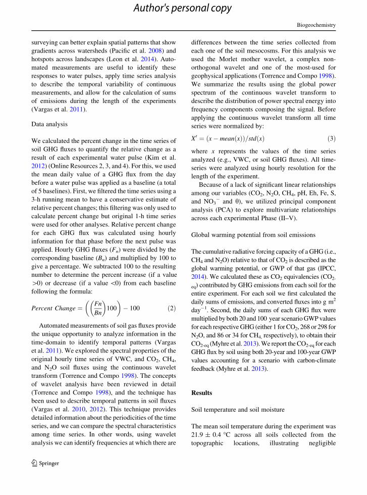
For the overall length of the experiment we found that
the Creek soil yielded the highest cumulative sum of
soil CO2 fluxes (314 g m-2) and the Wetland soil
yielded the lowest (160 g m-2, Fig. 4). Cumulative
sums of CH4 fluxes were highest from theWetland soil
Fig. 3 Principal
component analysis (PCA)
including fluxes of GHGs
(CO2 CH4, and N2O),
measurements of porewater
chemistry (Eh, pH, Fe, S,
NO3-), and volumetric
water content (h) for all soilsduring Phases II, III, IV, and
V (a, b, c, and d). Soils are
represented by colored
points: Purple represents the
Wetland, Green represents
the Creek, Red represents
Forest Site 1, and Blue
represents Forest Site 2.
(Color figure online)
Biogeochemistry
123
Author's personal copy
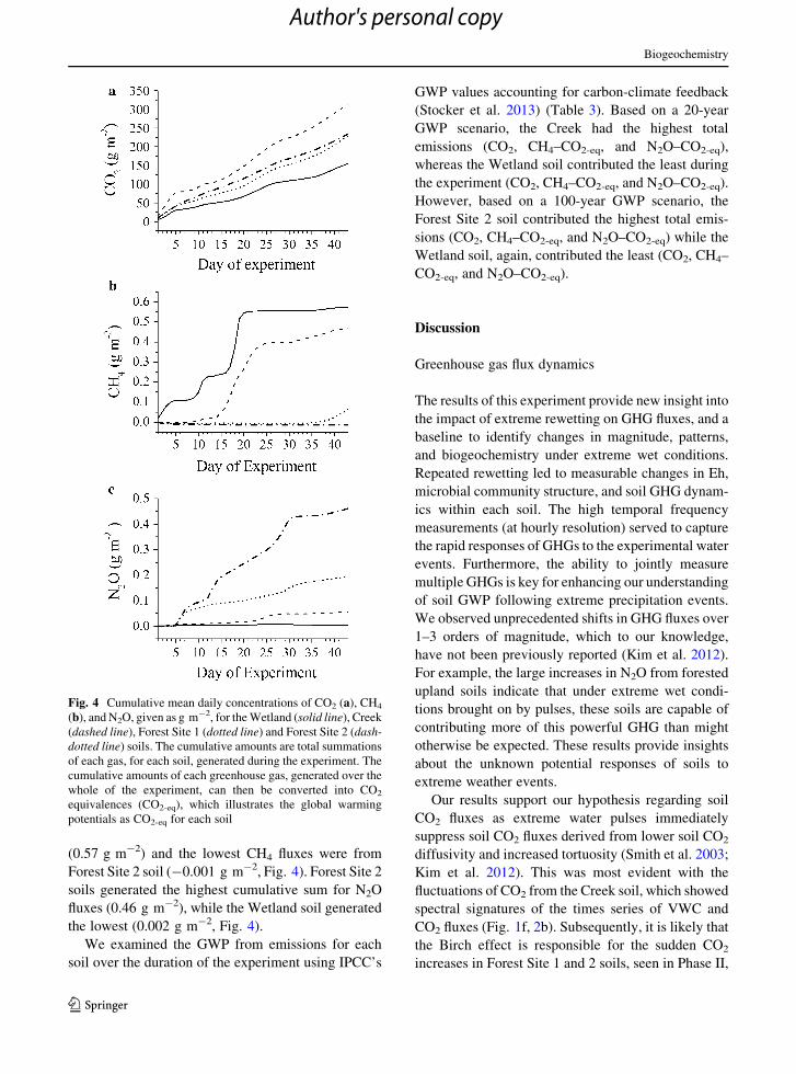
(0.57 g m-2) and the lowest CH4 fluxes were from
Forest Site 2 soil (-0.001 g m-2, Fig. 4). Forest Site 2
soils generated the highest cumulative sum for N2O
fluxes (0.46 g m-2), while the Wetland soil generated
the lowest (0.002 g m-2, Fig. 4).
We examined the GWP from emissions for each
soil over the duration of the experiment using IPCC’s
GWP values accounting for carbon-climate feedback
(Stocker et al. 2013) (Table 3). Based on a 20-year
GWP scenario, the Creek had the highest total
emissions (CO2, CH4–CO2-eq, and N2O–CO2-eq),
whereas the Wetland soil contributed the least during
the experiment (CO2, CH4–CO2-eq, and N2O–CO2-eq).
However, based on a 100-year GWP scenario, the
Forest Site 2 soil contributed the highest total emis-
sions (CO2, CH4–CO2-eq, and N2O–CO2-eq) while the
Wetland soil, again, contributed the least (CO2, CH4–
CO2-eq, and N2O–CO2-eq).
Discussion
Greenhouse gas flux dynamics
The results of this experiment provide new insight into
the impact of extreme rewetting on GHG fluxes, and a
baseline to identify changes in magnitude, patterns,
and biogeochemistry under extreme wet conditions.
Repeated rewetting led to measurable changes in Eh,
microbial community structure, and soil GHG dynam-
ics within each soil. The high temporal frequency
measurements (at hourly resolution) served to capture
the rapid responses of GHGs to the experimental water
events. Furthermore, the ability to jointly measure
multiple GHGs is key for enhancing our understanding
of soil GWP following extreme precipitation events.
We observed unprecedented shifts in GHG fluxes over
1–3 orders of magnitude, which to our knowledge,
have not been previously reported (Kim et al. 2012).
For example, the large increases in N2O from forested
upland soils indicate that under extreme wet condi-
tions brought on by pulses, these soils are capable of
contributing more of this powerful GHG than might
otherwise be expected. These results provide insights
about the unknown potential responses of soils to
extreme weather events.
Our results support our hypothesis regarding soil
CO2 fluxes as extreme water pulses immediately
suppress soil CO2 fluxes derived from lower soil CO2
diffusivity and increased tortuosity (Smith et al. 2003;
Kim et al. 2012). This was most evident with the
fluctuations of CO2 from the Creek soil, which showed
spectral signatures of the times series of VWC and
CO2 fluxes (Fig. 1f, 2b). Subsequently, it is likely that
the Birch effect is responsible for the sudden CO2
increases in Forest Site 1 and 2 soils, seen in Phase II,
Fig. 4 Cumulative mean daily concentrations of CO2 (a), CH4
(b), and N2O, given as g m-2, for theWetland (solid line), Creek
(dashed line), Forest Site 1 (dotted line) and Forest Site 2 (dash-
dotted line) soils. The cumulative amounts are total summations
of each gas, for each soil, generated during the experiment. The
cumulative amounts of each greenhouse gas, generated over the
whole of the experiment, can then be converted into CO2
equivalences (CO2-eq), which illustrates the global warming
potentials as CO2-eq for each soil
Biogeochemistry
123
Author's personal copy

as soil CO2 diffusivity increased, despite high VWC
levels (Fig. 1g, h; Birch 1958). This effect is also seen
in the Creek soil during Phase II (Fig. 1f). Overall, we
find that even after multiple large water pulses the
Creek soils show potential for rapidly recovered CO2
emissions, although the CO2 fluxes of all soils never
truly recover to what they were prior to the extreme
water pulses. These differences in magnitude and
temporal patterns of CO2 fluxes between each soil
draw attention to the importance of topographic
position, soil properties, and hydrological patterns to
the spatial variation of CO2 from soils (Pacific et al.
2009; Riveros-Iregui and McGlynn 2009; Leon et al.
2014).
Our results also support our hypothesis regarding
soil CH4 fluxes. We expected the Wetland and Creek
soils to act as an enhanced source of CH4 as is typical of
freshwater wetlands (Paul et al. 2006) and inundated
river floodplains (Pearson et al. 2016). Likewise, while
studies of temperate forests found upland forested soils
to be constant CH4 sinks, (Smith et al. 2003;Muhr et al.
2008; Erickson and Perakis 2014) our results support
the expectation that under extreme inundation these
soils shift from being a small CH4 sink to a small source
of CH4 to the atmosphere. Time series analysis
demonstrated the strong temporal response of Wetland
soil to experimental pulses, but a lack of temporal
consistency (i.e., no significant spectral signature;
Fig. 2c) for Forest site soils. Methane fluxes were
highest for the Wetland ([150 nmol m-2 s-1) and
Creek ([50 nmol m-2 s-1) soils during Phase III when
porewater S concentrations were the lowest (Table 1),
which is indicative of favorable conditions for
methanogenesis (Paul et al. 2006). In Phases IV and
V we observed an increase in porewater S and NO3-
from both of these soils. Therefore, we expect that
changes in Eh and sulfate reducing conditions pro-
moted sulfate reducing bacteria that may have outcom-
peted methanogenic microorganisms and consequently
decreased soil CH4 emissions, and the magnitude of
percent decrease in comparison to previous Phases. (Le
Mer and Roger 2001; Serrano-Silva et al. 2014). The
steady increase in CH4 fluxes (up to 10 nmol m-2 s-1)
from the Forest Site 1 soil during Phase V was
associated with a decrease in porewater NO3- suggest-
ing favorable conditions for methanogenesis (Fig. 1k).
In contrast, the increase in porewater NO3- fromForest
Site 2, coupled with higher N2O emissions and higher
porewater Fe concentrations, indicateNO3- and Fe(III)
reduction and unfavorable conditions for methanogen-
esis during Phase V. These observations support
findings from previous research where upland forest
soils decreased their long-term potential as CH4 sinks
under very wet conditions resulting from reduced
drainage (Christiansen et al. 2012).
We found evidence that soils with initial higher
NO3- (i.e., Forest Soils) resulted in larger N2O fluxes
following extreme rewetting events. Enhancement of
N2O fluxes from the wetting of Forest Site soils
supports previous evidence that forested soils can act
as large sources of N2O emissions (McDaniel et al.
2014) as they had higher initial concentrations of
porewater NO3- which likely promotes denitrifica-
tion. The magnitude of percent change in N2O fluxes
for Forest Site 1 and Forest Site 2 soils are unprece-
dented among previous reports for rewetting of soils
(Kim et al. 2012; McDaniel et al. 2014). During Phase
II we observed large increases of N2O fluxes within
both Forest site soils just hours after each pulse
addition. This may be a consequence of available
NO3- and labile dissolved organic matter as precur-
sors to denitrification leading to rapid and high
Table 3 The contributions of all GHGs in CO2-eq for each soil
(Wetland, Creek, Forest Site 1, Forest Site 2) over the entire
experiment for 20 and 100 year GWP scenarios, and the sum of
these equivalences (Total) for all GHGs: CO2 g m-2, CH4
g m-2 (CO2-eq), and N2O g m-2 (CO2-eq)
Soil CO2 g m-2 CH4 (CO2-eq) g m-2 N2O (CO2-eq) g m-2 Total (CO2-eq) g m-2
20 and 100 year
GWP scenario
20 year GWP
scenario
100 year
GWP scenario
20 year GWP
scenario
100 year
GWP scenario
20 year GWP
scenario
100 year
GWP scenario
Wetland 155.9 49.1 19.4 0.8 0.9 205.9 176.3
Creek 314.1 40.2 15.9 14.6 16.2 368.9 346.2
Forest Site 1 229.6 5.7 2.3 52.1 57.9 287.49 289.8
Forest Site 2 233.9 -1.2 -0.5 123.7 137.5 356.4 370.9
Biogeochemistry
123
Author's personal copy

responses of N2O fluxes (Enanga et al. 2015). Den-
itrification may have been limited in the Creek and
Wetland soils as a consequence of the low adsorption
capacity of NO3- in organic soils (Paul et al. 2006).
Initially, NO3- concentrations were high for Forest
Sites, but these shifted over the experiment to
comparable levels from the Wetland soil in Phase II.
Similar patterns of NO3- have also been observed in
upland humid tropical forest soils which experienced
prolonged inundation (Hall et al. 2013).
Relationships among variables
Overall, we did not find consistent significant linear
relationships between GHG fluxes, water content,
porewater chemistry, or other GHG fluxes, and our
results emphasize the complexity of the relationships
between biophysical conditions and production of
different GHGs from soils that have undergone
extreme rewetting events. Arguably, nonlinear models
more effectively describe complex dynamics of bio-
geochemical processes (Manzoni and Porporato
2009), but automated measurements provide unprece-
dented high temporal resolution information that is
difficult to fit into empirical models. Our results from
the wavelet analysis and PCA provide insight about
the temporal variation of soil GHG fluxes, and the
underlying biogeochemical controls of these fluxes.
The time series analysis revealed different period-
icities of soil GHG fluxes associated with the exper-
imental water additions, but continuous measurements
of other variables beyond temperature and VWC may
be needed to identify temporal coherency with this and
other soil GHG fluxes (Vargas et al. 2012). Previous
research has shown the importance of studying the role
of redox chemistry to understand the biogeochemical
drivers of GHG fluxes from soils (Yu et al. 2006; Hall
et al. 2013; McNicol and Silver 2014). Therefore,
automated Ehmeasurements in experiments and under
natural conditions are needed to better identify the
temporal coherency between this variable and soil
GHG fluxes.
A multivariate approach identified shifts on the
relative importance of biogeochemical variables
across the different soil types over the Phases of the
experiment (Fig. 3). Certain vectors in our PCA were
consistently associated with specific soil types. For
example, the Wetland soil was associated with S; this
could be explained by the potential presence of sulfate
reducing bacteria in these soils (Pester et al. 2012;
Serrano-Silva et al. 2014). Forest Site 1 and Forest Site
2 soils were consistently associated with N2O, likely
as a result of their sensitivity to soil conditions which
would promote denitrification (Pilegaard et al. 2006;
Chapin et al. 2011) and therefore the higher levels of
N2O fluxes from these soils. The Creek soil was
consistently associated with the highest porewater pH
values, which also increased over the duration of the
experiment. An increase in pH is associated with
decreasing electron activity (i.e., lower Eh) (Essington
2004; Grybos et al. 2009) and Fe(II) appears at a pH of
6.5 if electron activity is very low (Essington 2004),
potentially explaining why observed porewater Fe and
pH vectors were associated with the Creek soil in
Phase III (Fig. 3b).
During Phase V we observed convergence in the
multivariate space of the two Forest Site soils with a
strong association to porewater Fe and N2O (Fig. 3d).
Higher values of Fe and pH have been found in acidic,
waterlogged soils associated with reduction of NO3-
and Fe (Grybos et al. 2009). TheWetland soil remained
associated to S and Eh suggesting that extreme water
pulses have little effect on their biogeochemistry, as
these soils are typically associated with inundated
anoxic conditions (Zhuang et al. 2004). However,
drying of wetlands soils greatly impacts their biogeo-
chemistry by allowing for rapid turnover of labile
organic matter as the microbial community shifts to
aerobic metabolism, which may explain the 245%
increase in CO2 emissions during Phase V, when
compared to the suppressed CO2 fluxes during the very
wet conditions in Phase IV. (Figure 1a, e; Davidson
et al. 2014; McNicol and Silver 2015). In contrast, the
Creek soil substantially changed its association in the
multivariate space, indicative of the sensitivity of the
biogeochemistry of these soils in response to extreme
water pulse events. These soils are analogous to
floodplains that may undergo substantial rewetting
and drying events depending on runoff and water level,
therefore shifting their potential to become sink or
source of GHGs along the year (Pearson et al. 2016).
Microbial community shifts
Our results provide evidence that microbial commu-
nity structure can be rapidly influence by experimental
extreme water pulses under conditions of controlled
Biogeochemistry
123
Author's personal copy

temperature. Previous studies observed that microbial
community structure is sensitive to water stress
(Davidson et al. 1998; Schimel et al. 2007) and
changes in pH across ecosystems (Fierer and Jackson
1998). In our experiment, each soil began with a
distinct microbial community structure, but at the end
the microbial community structure of each soil had
shifted in different directions (in the multivariate
space of dimensions 1 and 2; Online Resource 6b).
While we initially thought that the community struc-
ture of the most predominant microorganisms would
become more similar following such extreme inunda-
tion. While the Creek, Forest Site 1, and Forest Site 2
soils do move towards one another, the Wetland soil
diverged from this trend. Ultimately, such a change
would influence geochemistry and GHG fluxes from
soils. The resulting changes in community structure
over a short period of time provide insights towards
the large challenge of predicting microbial community
responses to extreme weather events (Knapp et al.
2008; Evans and Wallenstein 2012).
We did not excise the DGGE bands for sequencing,
therefore we could not identify bacterial species
present on DGGE gel. DGGE is a quick fingerprinting
approach, which provides a ‘‘snapshot’’ on the dom-
inant bacteria from the community (Kan et al. 2006).
Most of the minor or rare species will be skipped from
the fingerprinting approaches such as DGGE. Deter-
mining the detailed bacterial community changes
would require (1) appropriate primers targeting at
specific groups of bacteria (e.g., methanogens,
methanotrophs, nitrifiers, denitrifiers etc.) or (2) more
detailed bacterial community characterization
approaches including high throughput sequencing
(Jenkins and Gibson 2002). Future studies targeting
methanogenic/methanotrophic and nitrifying/denitri-
fying groups of microorganisms could enhance under-
standing of patterns of CH4 and N2O seen from soils in
response to extreme weather events. These analyses,
in conjunction with environmental measurements
(e.g., GHG fluxes, physical conditions, and porewater
chemistry) could enhance our understanding of
ecosystem processes (Graham et al. 2016).
Global warming potential
GWP illustrates how extreme rewetting events might
influence the temporal dynamics of multiple GHGs
and how distinct soils might contribute to global
warming across complex terrain. This would not have
been possible without the use of automated measure-
ments, from which we calculated cumulative sums of
soil GHG fluxes, and determined the GWP in CO2-eq
from each GHG for each soil throughout the exper-
iment (Fig. 4; Table 3). The Creek soil had the most
CO2 efflux, the Wetland soil contributed the most CH4
efflux, and Forest Site 2 soil contributed the most N2O
efflux. With this information, we examined the GWP
for each soil using the 20-year and 100-year values
(Stocker et al. 2013) (Table 3). The Wetland soil was
responsible for the lowest GWP in comparison to other
soils because although CH4 has a higher radiative
forcing capacity, it is relatively short lived in the
atmosphere (Smith et al. 2003). Using 20-year GWP
values, we found the Creek contributed the most to the
total CO2-eq, as this soil had the largest fluxes of CO2,
and some CH4 and N2O. In contrast, when using the
100-year GWP values, we found that the Forest Site 2
soil had the largest impact as a result of increases of
N2O emissions, and highlights the important role of
N2O in temperate forested ecosystems (Enanga et al.
2015). These results emphasize the importance of
measuring multiple GHGs using automated measure-
ments to accurately calculate the GWP following
water pulses and extreme weather events.
Conclusions
High temporal frequency measurements of soil CO2,
N2O and CH4 fluxes (i.e., GHG fluxes) provided the
ability to explore rapid responses to experimental
water addition and accurately calculation of the GWP
of soils. We observed unprecedented changes in
magnitude of GHG fluxes, showing rapid changes in
soil GHG flux dynamics captured by automated
measurements. These high temporal measurements
provided insights on the temporal variation of these
emissions, but also highlight the challenge to represent
the responses of soil GHG fluxes following extreme
weather events. We observed shifts of the microbial
community structure between the beginning and end
of the experiment, indicating that extreme water
pulses can substantially impact microbial community
composition at short temporal scales (i.e.,\2 months).
Soil porewater chemistry provided insights on the
underlying biogeochemical mechanisms for produc-
tion and consumption of GHGs from soils, but we
Biogeochemistry
123
Author's personal copy

highlight a decoupling between passive manual sam-
ples and automated measurements. We propose that to
better understand the sensitivity of GHG fluxes to
changes in biogeochemical conditions (e.g., Eh), it
may be beneficial to incorporate a combination of
automated measurements to capture multiple GHG
fluxes and ancillary biogeochemical information.
Finally, we argue that because extreme events are
uncommon, the opportunities to capture ecosystem
responses are limited; therefore the use of experimen-
tal manipulation is an alternative way through which
we can advance our understanding of responses to
uncommon biophysical conditions. Consequently,
hypotheses pertaining to the responses of ecosystems
under the influence of extreme events can be tested and
reformulated, and models can be informed to better
parameterize responses with the ultimate goal of
improving their predictive capabilities for extreme
weather events.
Acknowledgements Funding was provided by the United
States Department of Agriculture-Agriculture and Food
Research Initiative (AFRI) Grants 2013-02758 and
2015-67020-23585, State of Delaware’s Federal Research and
Development Matching Grant Program, and endowment from
Stroud Water Research Center. We are grateful to William
Donahoe for his support to develop an R program to calculate
greenhouse gas fluxes. We are also grateful for the assistance of
Kelli Kearns, Erica Loudermilk, and Rattandeep Gill who
assisted with porewater extractions and analyses.
References
Birch HF (1958) The effect of soil drying on humus decompo-
sition and nitrogen availability. Plant Soil 10:9–31. doi:10.
1007/BF01343734
Borken W, Matzner E (2009) Reappraisal of drying and wetting
effects on C and N mineralization and fluxes in soils. Glob
Chang Biol 15:808–824. doi:10.1111/j.1365-2486.2008.
01681.x
Chapin FSI, Matson PA, Vitousek PM (2011) Principles of
terrestrial ecosystem ecology. Second, Springer New York
Christiansen JR, Gundersen P, Frederiksen P, Vesterdal L
(2012) Influence of hydromorphic soil conditions on
greenhouse gas emissions and soil carbon stocks in a
Danish temperate forest. For Ecol Manag 284:185–195.
doi:10.1016/j.foreco.2012.07.048
Creed IF, Beall FD (2009) Distributed topographic indicators
for predicting nitrogen export from headwater catchments.
Water Resour Res. doi:10.1029/2008WR007285
Dalal RC, Allen DE, Livesley SJ, Richards G (2008) Magnitude
and biophysical regulators of methane emission and con-
sumption in the Australian agricultural, forest, and sub-
merged landscapes: a review. Plant Soil 309(1–2):43–76
Davidson EA (1992) Pulses of nitric oxide and nitrous oxide flux
following wetting of dry soil: an assessment of probable
sources and importance relative to annual fluxes. Ecol Bull
42:149–155
Davidson E, Belk E, Boone RD (1998) Soil water content and
temperature as independent or confounded factors con-
trolling soil respiration in a temperate mixed hardwood
forest. Glob Chang Biol 4:217–227. doi:10.1046/j.1365-
2486.1998.00128.x
Davidson EA, Savage KE, Finzi AC (2014) A big-microsite
framework for soil carbon modeling. Glob Chang Biol
20:3610–3620. doi:10.1111/gcb.12718
Dhillon GS, Inamdar S (2013) Extreme storms and changes in
particulate and dissolved organic carbon in runoff: entering
uncharted waters? Geophys Res Lett 40:1322–1327.
doi:10.1002/grl.50306
Enanga EM, Creed IF, Casson NJ, Beall FD (2015) Summer
storms trigger soil N2O efflux episodes in forested catch-
ments. J Geophys Res Biogeosci. doi:10.1002/
2015JG003027
Erickson HE, Perakis SS (2014) Soil fluxes of methane, nitrous
oxide, and nitric oxide from aggrading forests in coastal
Oregon. Soil Biol Biochem 76:268–277. doi:10.1016/j.
soilbio.2014.05.024
Essington ME (2004) Soil and water chemistry an integrative
approach. CRC Press, Boca Raton
Evans SE, Wallenstein MD (2012) Soil microbial community
response to drying and rewetting stress: does historical
precipitation regime matter? Biogeochemistry
109:101–116. doi:10.1007/s10533-011-9638-3
Fierer N, Jackson RB (1998) The diversity and biogeography of
soil bacterial communities. PNAS 103:626–631. doi:10.
1073/pnas.0507535103
Fierer N, Schimel JP (2002) Effects of drying–rewetting fre-
quency on soil carbon and nitrogen transformations. Soil
Biol Biochem 34:777–787. doi:10.1016/S0038-
0717(02)00007-X
Frank D, Reichstein M, Bahn M et al (2015) Effects of climate
extremes on the terrestrial carbon cycle: concepts, pro-
cesses and potential future impacts. Glob Chang Biol
21:2861–2880. doi:10.1111/gcb.12916
Gorres C-M, Kammann C, Ceulemans R (2016) Automation of
soil flux chamber measurements: potentials and pitfalls.
Biogeosci Discuss 12:14693–14738. doi:10.5194/bgd-12-
14693-2015
Graham EB, Knelman JE, Schindlbacher A et al (2016)
Microbes as engines of ecosystem function: when does
community structure enhance predictions of ecosystem
processes? Front Microbiol 7:1–10. doi:10.3389/fmicb.
2016.00214
Grybos M, Davranche M, Gruau G et al (2009) Increasing pH
drives organic matter solubilization from wetland soils
under reducing conditions. Geoderma 154:13–19. doi:10.
1016/j.geoderma.2009.09.001
Hall S, McDowell W, Silver W (2013) When wet gets wetter:
decoupling of moisture, redox biogeochemistry, and
greenhouse gas fluxes in a humid tropical forest soil.
Ecosystems 16:576–589. doi:10.1007/s10021-012-9631-2
Haugwitz MS, Bergmark L, Prieme A et al (2014) Soil
microorganisms respond to five years of climate change
manipulations and elevated atmospheric CO2 in a
Biogeochemistry
123
Author's personal copy

temperate heath ecosystem. Plant Soil 374:211–222.
doi:10.1007/s11104-013-1855-1
Jarvis P, Rev A, Petsikos C et al (2007) Drying and wetting of
Mediterranean soils stimulates decomposition and carbon
dioxide emission: the ‘‘Birch effect’’. Tree Physiol
27:929–940
Jenkins S, Gibson N (2002) High-throughput SNP genotyping.
Comp Funct Genomics 3:57–66. doi:10.1002/cfg.130
Kan J,WangK, Chen F (2006) Temporal variation and detection
limit of an estuarine bacterioplankton community analyzed
by denaturing gradient gel electrophoresis (DGGE). Aquat
Microb Ecol 42:7–18. doi:10.3354/ame042007
Kayler ZE, DeBoeck HJ, Fatichi S et al (2015) Experiments to
confront the environmental extremes of climate change.
Front Ecol Environ 13:219–225
Kim D-G, Vargas R, Bond-Lamberty B, Turetsky MR (2012)
Effects of soil rewetting and thawing on soil gas fluxes: a
review of current literature and suggestions for future
research. Biogeosciences 9:2459–2483. doi:10.5194/bg-9-
2459-2012
Klironomos JN, Rillig MC, Allen MF (1999) Designing
belowground field experiments with the help of semi-
varience and power analysis. Appl Soil Ecol 12:227–238
Knapp AK, Beier C, Briske DD et al (2008) Consequences of
more extreme precipitation regimes for terrestrial ecosys-
tems. Bioscience 58:811. doi:10.1641/B580908
Lado-Monserrat L, Lull C, Bautista I et al (2014) Soil moisture
increment as a controlling variable of the ‘‘Birch effect’’.
Interactions with the pre-wetting soil moisture and litter
addition. Plant Soil 379:21–34. doi:10.1007/s11104-014-
2037-5
Le Mer J, Roger P (2001) Production, oxidation, emission and
consumption of methane by soils: a review. Eur J Soil Biol
37(1):25–50
Leon E, Vargas R, Bullock S et al (2014) Hot spots, hot
moments, and spatio-temporal controls on soil CO2 efflux
in a water-limited ecosystem. Soil Biol Biochem 77:12–21.
doi:10.1016/j.soilbio.2014.05.029
Liengaard L, Nielsen LP, Revsbech NP et al (2013) Extreme
emission of N2O from tropical wetland soil (Pantanal,
South America). Front Microbiol 3:433
Manzoni S, Porporato A (2009) Soil carbon and nitrogen min-
eralization: theory and models across scales. Soil Biol
Biochem 41:1355–1379. doi:10.1016/j.soilbio.2009.02.
031
McDaniel MD, Kaye JP, Kaye MW (2014) Do ‘‘hot moments’’
become hotter under climate change? Soil nitrogen
dynamics from a climate manipulation experiment in a
post-harvest forest. Biogeochemistry 121:339–354. doi:10.
1007/s10533-014-0001-3
McNicol G, Silver WL (2014) Separate effects of flooding and
anaerobiosis on soil greenhouse gas emissions and redox
sensitive biogeochemistry. J Geophys Res Biogeosciences
119:557–566. doi:10.1002/2013JG002433.Received
McNicol G, Silver WL (2015) Non-linear response of carbon
dioxide and methane emissions to oxygen availability in a
drained histosol. Biogeochemistry 123:299–306. doi:10.
1007/s10533-015-0075-6
Muhr J, Goldberg S, Borken W, Gebauer G (2008) Repeated
drying–rewetting cycles and their effects on the emission
of CO2, N2O, NO, and CH4 in a forest soil. J Plant Nutr Soil
Sci 171:719–728. doi:10.1002/jpln.200700302
Muyzer G, De Waal EC, Uitterlinden AG (1993) Profiling of
complex microbial populations by denaturing gradient gel
electrophoresis analysis of polymerase chain reaction-
amplified genes coding for 16S rRNA. Appl Environ
Microbiol 59:695–700
Myhre G, Shindell D, Breon F-M et al (2013) 2013: anthro-
pogenic and natural radiative forcing. In: Stocker TF, Qin
D, Plattner G-K, et al. (eds) Climate change 2013: the
physical science basis. Contribution of working group I to
the fifth assessment report of the intergovernmental panel
on climate change. Cambridge University Press, Cam-
bridge, pp 659–740
Pachauri RK, Allen MR, Barros VR et al (2014) IPCC, 2014:
climate change 2014 synthesis report summary for poli-
cymakers. Cambridge, United Kingdom
Pacific VJ, McGlynn BL, Riveros-Iregui DA et al (2008)
Variability in soil respiration across riparian-hillslope
transitions. Biogeochemistry 91:51–70. doi:10.1007/
s10533-008-9258-8
Pacific VJ, McGlynn BL, Riveros-Iregui DA et al (2009) Dif-
ferential soil respiration responses to changing hydrologic
regimes. Water Resour Res 45:6–11. doi:10.1029/
2009WR007721
Paul S, Kusel K, Alewell C (2006) Reduction processes in forest
wetlands: tracking down heterogeneity of source/sink
functions with a combination of methods. Soil Biol Bio-
chem 38:1028–1039. doi:10.1016/j.soilbio.2005.09.001
Pearson AJ, Pizzuto JE, Vargas R (2016) Influence of run of
river dams on floodplain sediments and carbon dynamics.
Geoderma 272:51–63. doi:10.1016/j.geoderma.2016.02.
029
Pester M, Knorr KH, Friedrich MW et al (2012) Sulfate-re-
ducing microorganisms in wetlands—fameless actors in
carbon cycling and climate change. Front Microbiol
3:1–19. doi:10.3389/fmicb.2012.00072
Pilegaard K, Skiba U, Ambus P et al (2006) Factors controlling
regional differences in forest soil emission of nitrogen
oxides (NO and N2O). Biogeosciences 3:651–661
Riveros-Iregui DA, McGlynn BL (2009) Landscape structure
control on soil CO2 efflux variability in complex terrain:
scaling from point observations to watershed scale fluxes.
J Geophys Res Biogeosci. doi:10.1029/2008JG000885
Savage KE, Davidson EA (2003) A comparison of manual and
automated systems for soil CO2 flux measurements: trade-
offs between spatial and temporal resolution. J Exp Bot
54:891–899. doi:10.1093/jxb/erg121
Savage K, Phillips R, Davidson E (2014) High temporal fre-
quency measurements of greenhouse gas emissions from
soils. Biogeosciences 11:2709–2720. doi:10.5194/bg-11-
2709-2014
Schimel J, Balser TC, Wallenstein M (2007) Microbial stress-
response physiology and its implications for ecosystem
function. Ecology 88:1386–1394. doi:10.1890/06-0219
Schlesinger W, Andrews J (2000) Soil respiration and the global
carbon cycle. Biogeochemistry 48:7–20. doi:10.1023/A:
1006247623877
Serrano-Silva N, Sarria-Guzman Y, Dendooven L, Luna-Guido
M (2014) Methanogenesis and methanotrophy in soil: a
Biogeochemistry
123
Author's personal copy

review. Pedosphere 24:291–307. doi:10.1016/S1002-
0160(14)60016-3
Seyfferth AL, Fendorf S (2012) Silicate mineral impacts on the
uptake and storage of arsenic and plant nutrients in rice
(Oryza sativa L.). Environ Sci Technol 46:13176–13183.
doi:10.1021/es3025337
Smith KA, Ball T, Conen F et al (2003) Exchange of green-
housegases between soil and atmosphere: interactions of
soil physical factors and biological processes. Eur J Soil Sci
54:779–791. doi:10.1046/j.1365-2389.2003.00567.x
Steduto P, Cetinkoku O, Albrizio R, Kanber R (2002) Auto-
mated closed-system canopy-chamber for continuous field-
crop monitoring of CO2 and H2O fluxes. Agric For Mete-
orol 111:171–186. doi:10.1016/S0168-1923(02)00023-0
Stocker TF, Qin D, Plattner G-K et al (2013) IPCC, 2013: cli-
mate change 2013: the physical science basis, contribution
of working group I to the fifth assessment report of the
intergovernmental panel on climate change. Cambridge,
United Kingdom
Sutherland WJ, Freckleton RP, Godfray HCJ et al (2013)
Identification of 100 fundamental ecological questions.
J Ecol 101:58–67. doi:10.1111/1365-2745.12025
Torrence C, Compo GP (1998) A practical guide to wavelet
analysis. Bull Am Meteorol Soc 79:61–78. doi:10.1175/
1520-0477(1998)079\0061:APGTWA[2.0.CO;2
Vargas R (2012) How a hurricane disturbance influences
extreme CO2 fluxes and variance in a tropical forest.
Environ Res Lett 7:35704. doi:10.1088/1748-9326/7/3/
035704
Vargas R, Detto M, Baldocchi DD, Allen MF (2010) Multiscale
analysis of temporal variability of soil CO2 production as
influenced by weather and vegetation. Glob Chang Biol
16:1589–1605. doi:10.1111/j.1365-2486.2009.02111.x
Vargas R, Carbone MS, Reichstein M, Baldocchi DD (2011)
Frontiers and challenges in soil respiration research: from
measurements to model-data integration. Biogeochemistry
102:1–13. doi:10.1007/s10533-010-9462-1
Vargas R, Collins SL, Thomey ML et al (2012) Precipitation
variability and fire influence the temporal dynamics of soil
CO2 efflux in an arid grassland. Glob Chang Biol
18:1401–1411. doi:10.1111/j.1365-2486.2011.02628.x
Warner DL, Villarreal S, McWilliams K et al (2016) Carbon
dioxide and methane fluxes from tree stems, coarse woody
debris, and soils in an upland temperate forest. Ecosyst.
doi:10.1007/s10021-016-0106-8
Xu X, Luo X (2012) Effect of wetting intensity on soil GHG
fluxes and microbial biomass under a temperate forest floor
during dry season. Geoderma 170:118–126. doi:10.1016/j.
geoderma.2011.11.016
Yu K, Faulkner SP, Patrick WH (2006) Redox potential char-
acterization and soil greenhouse gas concentration across a
hydrological gradient in a Gulf coast forest. Chemosphere
62:905–914. doi:10.1016/j.chemosphere.2005.05.033
Zhuang Q, Zhu X, He Y et al (2004) In fl uence of changes in
wetland inundation extent on net fl uxes of carbon dioxide
and methane in northern high latitudes from 1993 to 2004.
Environ Res Lett 10:95009. doi:10.1088/1748-9326/10/9/
095009
Biogeochemistry
123
Author's personal copy