author's personal copy - naval postgraduate school...

This article appeared in a journal published by Elsevier. The attachedcopy is furnished to the author for internal non-commercial researchand education use, including for instruction at the authors institution

and sharing with colleagues.

Other uses, including reproduction and distribution, or selling orlicensing copies, or posting to personal, institutional or third party

websites are prohibited.

In most cases authors are permitted to post their version of thearticle (e.g. in Word or Tex form) to their personal website orinstitutional repository. Authors requiring further information

regarding Elsevier’s archiving and manuscript policies areencouraged to visit:

http://www.elsevier.com/copyright

http://www.elsevier.com/copyright

Author's personal copy

Nutrient pumping/advection by propagating Rossby Waves in theKuroshio Extension

Peter C. Chu n, Yu-Heng Kuo

Department of Oceanography, Naval Postgraduate School, Monterey, CA 93943, USA

a r t i c l e i n f o

Article history:

Received 22 April 2010

Accepted 22 April 2010Available online 29 April 2010

Keywords:

Rossby wave propagation

Kuroshio extention

Nutrient pumping/advection

Meso-scale eddies

Sea level anomaly

Chlorophyll-a concentration

a b s t r a c t

Ten years (1998–2007) of sea-level anomalies (SLA) from multiple satellite altimeters and chlorophyll-a

concentration from the Sea-viewing Wide Field-of-view Sensor (SeaWiFS) were used to detect eddy

pumping/advection of nutrients by the action of propagating Rossby waves in the Kuroshio Extension

(KE) region near 35oN after the seasonal SeaWiFS chlorophyll-a (Chl-a) concentrations cycles and

annual changes of altimeter SLA were eliminated. Spatial structure of Chl-a anomalies to the seasonal

cycle is examined in relation to altimeter eddy structure. Eddy propagation speeds and scales by the

Rossby waves are also identified. Chl-a structure is evident during the spring bloom period with a scale

around 460 km. Cold-core (cyclonic) rings correspond to areas of high Chl-a concentrations. Warm-core

(anticyclonic) rings relate to areas of low Chl-a concentration. Chl-a anomalies and SLA have an overall

modest negative correlation coefficient of r¼�0.45, which may imply the co-existence of both eddy

pumping and eddy advection mechanisms in the KE region. Swirl currents between eddies redistribute

surface chlorophyll concentrations and can spatially bias maximum and minimum concentration levels

off eddy center. The correlation coefficient has seasonal fluctuations. In the western KE region, it varies

from high negative correlation (r¼�0.70) in April and September (eddy pumping dominant) to low

negative correlation (r¼�0.33) in February and March (eddy advection dominant). In the eastern KE

region, it varies from high negative correlation (r¼�0.67) in February to low negative correlation

(r¼�0.42) in December. It is noted that the characteristic wavelengths of the SLA and Chl-a features,

and the seasonality of the correlation between these two variables have not been previously

documented.

Published by Elsevier Ltd.

1. Introduction

Primary productivity in the open ocean is limited by the lack ofnutrients in surface waters. These nutrients are mostly suppliedfrom nutrient-rich subsurface waters through upwelling andvertical mixing (Barber, 1992). Vertical diffusivity was found to berelated to primary production near the top of the SubtropicalMode Water (STMW) in the western North Pacific (Sukigara et al.,2009). Seasonal and intra-seasonal variability of SeaWiFS chlor-ophyll-a (Chl-a) in the North Pacific was identified using modeland satellite data and the response of the biological production tothe uplift and depression of the nutricline with the variability ofmesoscale physical phenomena (Sasai et al., 2007). However, inthe ocean gyres these mechanisms do not fully account for theobserved productivity (Jenkins and Goldman, 1985). Variousmechanisms have been proposed for explaining the primaryproductivity. Among them, upward pumping and horizontal

advection of nutrients through the action of eddies are mostpopular. For example, upward pumping to account for theremainder of the primary productivity was identified fromsatellite data in regional seas such as Sargasso Sea (e.g., Siegelet al., 1999) and North Pacific Ocean (Uz et al., 2001). Afteranalyzing the coherence between sea-level anomalies (SLA) andChl-a from satellite data, Uz et al. (2001) claimed the importanceof pumping mechanism with westward propagating Rossbywaves for the Chl-a structure. Chu and Fang (2003) also detectedthe Rossby wave propagation in the South China Sea from satellitealtimetry data. The eddy swirl currents also advect phytoplanktonconcentrations at rates less, comparable or greater than thepropagation rates of concentration structures due to phytoplank-ton growth dynamics. At external regions, chlorophyll structurecan be moved between eddies and so chlorophyll can be mixedacross concentration gradients (Leterme and Pingree, 2008).

Thus, two competing mechanisms, eddy pumping and eddyadvection, co-exist. The eddy pumping mechanism causes highChl-a concentration anomaly co-located with the cyclonic eddy;and low Chl-a concentration anomaly is co-located with theanticyclonic eddy. The eddy advection mechanism causes mixing

Contents lists available at ScienceDirect

journal homepage: www.elsevier.com/locate/dsr2

Deep-Sea Research II

0967-0645/$ - see front matter Published by Elsevier Ltd.

doi:10.1016/j.dsr2.2010.04.007

n Corresponding author.

E-mail address: [email protected] (P.C. Chu).

Deep-Sea Research II 57 (2010) 1809–1819


between high- and low-Chl-a regions. If the pumping mechanismdominates, the negative correlation between SLA and Chl-a

concentration anomaly is high. If advection mechanism dom-inates, the negative correlation between SLA and Chl-a concen-tration anomaly is low.

In this study, 10 years (1998–2007) of SLA from multiplesatellite altimeters and Chl-a concentration from the Sea-viewingWide Field-of-view Sensor (SeaWiFS) were used to detecteddy pumping/eddy advection of nutrients by the action ofpropagating 2.

2. Kuroshio Extension

The Oyashio Current water is formed by East KamchatkaCurrent water and Okhotsk Sea water modified by mixing in theKuril straits. It flows southwestward along the Kuril Islands andturns eastward from the northern coast of Japan. The Kuroshioflows northward from the tropical area to Tohoku area east ofJapan. The Kuroshio turns eastward from the eastern coast ofHonshu, Japan, and the strong eastward flow around 35oN iscalled the KE (mid-latitude western boundary current outflowregion), which is the continuation of the warm, northward-flowing waters of the Kuroshio western boundary current, andforms a vigorously meandering boundary between the warmsubtropical and cold northern waters of the Pacific. The warmKuroshio waters encounter the cold dry air masses coming fromthe Asian continent, and create intense air sea heat exchanges inthe KE region. Solomon (1978) discovered a current ring detachedfrom the large quasi-steady Kuroshio meander south of Honshu inMay 1977. The ring remained stationary until August, when itrecombined with the main Kuroshio to reform a meanderdistorted in shape and upstream from the original meander.Meanders which separate northward of the KE jet generateanticyclonic (warm-core) eddies and those which separate south-ward of the KE jet produce cyclonic (cold-core) eddies. The warm-core eddies on the northern side are originated mostly from thearea of Sanriku, and the cold-core eddies on the southern side aremainly generated from the area off the Boso Peninsula (Sun et al.,1989). A complete life history of cyclonic ring was observed: asouthward meander of the KE jet, its pinching-off to form a

cyclonic ring, the ring’s westward movement, its coalescence withthe KE jet (Ichikawa and Imawaki, 1994).

Fig. 1 shows two quasi-stationary meanders with their ridgeslocated at 144 and 1501E exist along the mean path of theupstream KE (Qiu and Chen, 2005). A tight recirculation gyre islocated south of the quasi-stationary meanders of the KE jet, andincreases the eastward transport of the KE from near 50 Sv toabout 130 Sv (where 1 Sv¼106 m3 s�1). Near 1591E, the KE jetencounters the Shatsky Rise where it often bifurcates: the mainbody of the jet continues eastward, and a secondary branch tendsto move northeastward to 401N where it joins the SubarcticCurrent (e.g., Mizuno and White, 1983; Niiler et al., 2003). Withthe broadening in its width downstream of 1601E, the KE loses itsinertial jet characteristics and rejoins gradually the interiorSverdrup circulation as the North Pacific Current.

Remotely sensed data collected since the late 1970s providesoceanographers with a large volume of information on the state ofthe surface of the World Ocean. Qiu and Chen (2005) analyzedtwelve years of SLA from multiple satellite altimeters. In the KEregion, part of SLA measured by the altimeters reflects theseasonally varying surface heat flux that causes expansion orcontraction of the water column (e.g., Stammer, 1997; Gilsonet al., 1998). Qiu and Chen (2005) removed these steric heightchanges from the weekly SLA dataset and investigated the low-frequency changes and the interconnections of the KE jet, itssouthern recirculation gyre, and their mesoscale eddy field.Following Qiu and Chen (2005), the axis of the KE jet is definedby the 170-cm sea surface height contours, which are consistentlylocated at, or near, the maximum of its latitudinal gradient(Fig. 2).

3. Methods and data

3.1. SLA

SLA heights have been measured by the ERS 1/2 and TOPEX/Poseidon satellites from 1 January 1998 to 31 December 2007 at7-day intervals. Radar altimeters on board the satellite continu-ally transmit signals at high frequencies to Earth and receivereflected signals from the sea surface. The data have been

Fig. 1. Surface dynamic height field (cm; white contours) relative to 1000 dbar from Teague et al. (1990). Colored map shows the bathymetry based on Smith and Sandwell

(1994). Major bathymetric features in the region include the Izu–Ogasawara Ridge along 6.401E and the Shatsky Rise around 1591E (after Qiu and Chen 2005).

P.C. Chu, Y.-H. Kuo / Deep-Sea Research II 57 (2010) 1809–18191810


processed according to Le Traon et al. (1998) with SLA spatiallyinterpolated to 0.251 in both latitude and longitude. Maps of SLAwere derived for the North Pacific to compare with monthlycomposites of Chl-a concentration.

SLA has evident annual cycle and mesoscale structuredominated by eddy or Rossby waves. The annual signal isinfluenced partially by the ocean circulation and partially by therise and fall of the sea surface that arises from the expansion andcontraction of the ocean due to its heating and cooling withseasonal change. The region of large variance of sea-surface heightin the North Pacific is along the mean KE jet (represented by170-cm contour in Fig. 1), where the annual buoyancy andrecirculation changes cause a maximum annual elevation changeof about 720 cm (Fig. 2). Since we are interested in elevationstructure that correlates with non-seasonal Chl-a structure, theannual component and any residual mean elevation removedfrom the SLA data using the Fourier analysis. Although relativelysmall in this context, aliasing due to the semi-diurnal tide is alsoremoved. We refer to the resulting data as SLA residuals. Themean KE jet selected is a few degrees north of the maximumannual amplitude of SLA (Fig. 2) and other spectral componentstended to show similar distributions of amplitude structure.

Altimeter and Chl-a data are also extracted every 0.251 alongthe mean KE axis (corresponding to 80 stations sampled over adistance of 1820 km; Fig. 3) from January 1998 to December 2007(10-year period). Temporal variations of sea-surface elevationresiduals and Chl-a along the mean KE axis are plotted on time-longitude cross-sections. An overlapping time window of Chl-a

anomalies and altimeter residuals is compared.

3.2. Chl-a

Chl-a data were obtained from the Goddard Distributed ActiveArchive Center under the auspices of NASA. Use of these data is in

accordance with the SeaWiFS Research Data User Terms andConditions Agreement. The SeaDAS software was used to computeChl-a concentration (Ca) from the ratio of radiances measured inband-3 (480–500 nm) and band-5 (545–565 nm) according to thefollowing NASA algorithm,

Ca ¼ exp½0:464�1:989LnðLWM490=LWM555Þ�, ð1Þ

and monthly composite Chl-a maps for the North Pacific werederived. For deriving the 10-year mean seasonal cycles, the Chl-a

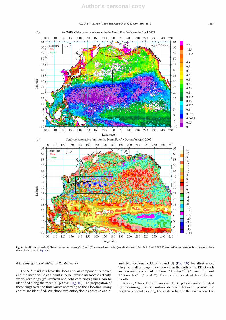
data are spatially averaged over 725 km in both latitude andlongitude and missing data due to cloud coverage interpolated.For example, Fig. 4 shows the Chl-a structure and SLA residual inApril 2007. The velocities were determined using the geostrophicrelation from SLA residual map (Fig. 4B). To examine the eddyeffect on Chl-a structure, seasonal cycles were removed from theChl-a and SLA data. The Chl-a anomalies or residuals werecompared to the SLA residuals from January 1998 to December2007.

4. Results

4.1. Structure of Chl-a and SLA

The Chl-a monthly composite for April 2007 shows the springbloom boundary arbitrarily defined by concentration levels of0.2 mg m�3 Chl-a concentrations (Fig. 4A). The boundary is notregular but has perturbations due to eddy structure. The NorthPacific SLA map for April 2007 (Fig.4B) shows the correspondingmesoscale eddy field. The main open-ocean dynamical influenceson the Chl-a field are vertical pumping and/or horizontaladvection by eddies with a length scale around 460 km.

To identify the association between spatial patterns of eddyand Chl-a concentrations for the KE extension area (rectangularbox in Fig. 4), we re-plot Chl-a concentrations (in color) and SLA

Longitude

100

Annual Sea Level amplitude (mm) in the North Pacific Ocean

-10

-5

0

5

10

15

20

25

30

35

40

45

50

55

60

65

Lat

itude

-10

-5

0

5

10

15

20

25

30

35

40

45

50

55

60

65(mm)

0

10

20

30

40

50

60

70

80

90

100

120

160

NOAP NPGS

110 120 130 140 150 160 170 180 190 200 210 220 230 240 250

100 110 120 130 140 150 160 170 180 190 200 210 220 230 240 250

Fig. 2. Annual sea-level amplitude (mm) in the North Pacific Ocean. The Kuroshio Extension route selected (marked blank) along the 170 cm SSH contour (see Fig. 1), which

is associated with large amplitude region.

P.C. Chu, Y.-H. Kuo / Deep-Sea Research II 57 (2010) 1809–1819 1811


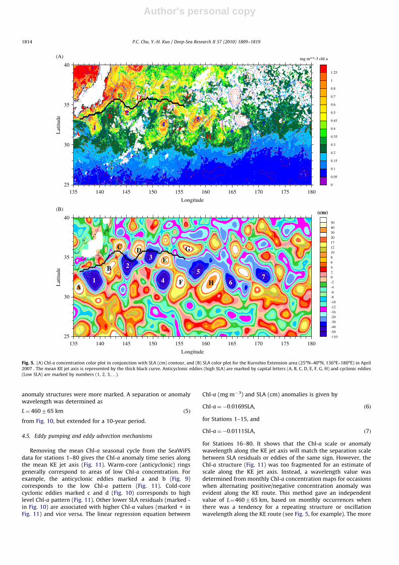
(in contour) in Fig. 5. High SLA values (anticyclonic eddies) areindicated by capital letters (A, B, C, D, E, F, G, H), and low SLAvalues (cyclonic eddies) are marked as numerical numbers (1, 2,3,y). Cyclonic (anticyclonic) eddies are co-located with high(low) Chl-a concentration areas.

At Station-1 (136.25oE, 33.25oN) (see Fig. 3), the beginning ofthe KE jet, Chl-a concentratiosn have an evident seasonal cyclewith a strong spring bloom (March-April) and a weak fall bloom(Fig. 6) with a maximum Chl-a concentration of 0.97 mg m�3 inApril 2000 and a minimum Chl-a concentration of 0.12 mg m�3 inSeptember 2007. Chl-a concentrations start to increase in thewinter period (after September) as the mixed layer deepens dueto winter mixing (with nutrient renewal). The sea-surfacetemperature (SST) on the KE Observatory mooring sitenominally at 32.4oN, 144.6oE (see website: http://www.pmel.noaa.gov/keo/data.html) shows that the bloom maximumoccurred in April (see Fig. 9) early during the development ofthe seasonal thermocline. The combination of modeststratification and nutrients left over from the winter mixingallows rapid phytoplankton growth near the surface.

4.2. Fluctuations of Chl-a and SLA along the mean KE jet axis

Inspection of both SLA and Chl-a maps show more intensespatial structure in the KE region. Mean and variance of Chl-a

concentrations (Fig. 7) and variance of SLA (Fig. 8) are calculatedat all stations (1–80) nearly 0.251 apart along the mean KE jet axis.There is a significant difference in Chl-a concentrations betweenstations 1 and 15 and stations 16 and 80. The mean Chl-a

concentration is estimated as

xChl a7s¼ 0:3770:02 mg m�3 ð2Þ

for stations 1 to 15, which is higher than

xChla7s¼ 0:2870:02 mg m�3 ð3Þ

for stations 16 to 80. The difference in Chl-a is likely due to thechanging properties along the mean KE axis. Between stations 1and 15, at the beginning of the KE jet, the water is more in theproximity of the coast that leads to greater nutrient fluxes to theeuphotic zone. The monthly distribution maps show that highChl-a inflow off Japan coast is most evident in April (see Fig. 5).The SLA shows high fluctuations in variance along the KE axis(Fig. 8),

s2SLA ¼ 8707460 cm2: ð4Þ

The maximum variance of 1800 cm2 corresponds to a rootmean squared fluctuation of sea level of about 742 cm on the

mean KE jet axis. The SLA variance increases generally from186 cm2 at Station-1 (33.25oN, 136.25oE) to near 1770 cm2

at Station-36 (34.75oN, 145oE). Small SLA variance valuesmight represent a regular pattern of nodes or a meander scaleextending 600 km from the position where the KE jet leavesJapanese coast.

4.3. Two seasonal blooms in the KE region

Chl-a structure in space and time may be masked by adominant seasonal cycle so the Chl-a anomalies or residuals aredefined as differences from a mean seasonal cycle. The seasonalcycles obtained for stations 1 to 15 (horizontal scale � 500 km)and stations 16 to 80 (horizontal scale �1500 km) are shown inFig. 9. Two peaks in the annual Chl-a cycle, spring and fall bloomsare mainly determined by light and nutrient limitation,respectively. Just below a euphotic layer the concentration ofnutrients increase with depth. On such large horizontal scales,vertical stability is a major factor to affect the nutrient limitationand vertical position of phytoplankton (two opposite effects onphytoplankton concentration). Usually, strong (weak) verticalstability reduces (increases) the nutrient supply and allows(disallows) phytoplankton to stay in the euphotic layer. Inwinter (December-February), the ocean surface mixed layer isdeep. Weak vertical stability does not allow phytoplankton to stayin the euphotic layer, which causes low production (low values ofChl-a in Fig. 9) since phytoplankton cannot obtain light enoughfor growth even with a high nutrient supply. As springapproaches, vertical stability strengthens; phytoplankton canstay in the euphotic layer long enough to grow with reduced(but sufficient) nutrient supply from the winter, so that a springbloom starts and reaches maximum production in April(0.55 mg m�3 Chl-a). In summer (June - August), the watercolumn is too stable. Strong vertical stability limits the nutrientsupply from deep water, which causes low production with aminimum value in August (0.25 mg m�3 Chl-a for stationsbetween 1 and 15, and 0.15 mg m�3 Chl-a for stations between16 and 80), since phytoplankton cannot get sufficient nutrientseven staying the euphotic layer. As fall approaches, the verticalstability weakens; supply of nutrients from deep water increases.Phytoplankton is still within the euphotic layer. This leads to asecond bloom in November (0.43 mg m�3 Chl-a for stationsbetween 1 and 15, and 0.30 mg m�3 Chl-a for stations between 16and 80). Thus, the spring bloom results from increased light levelsand the autumn bloom are a response to nutrient availability dueto increased vertical mixing and seasonal thermocline erosion.

135 140 145 150 155 160 165 170 175 180

Longitude °E

25

27

29

31

33

35

37

39

Lat

itud

e °N

200 m500 m1000 m2000 m

3000 m4000 m5000 mCoastline

1

80

40

15

Fig. 3. Topography of the studied area and Kuroshio Extension axis (marked orange) adopted for the present study. Stations positions 1, 15, 40 and 80 are marked.



4.4. Propagation of eddies by Rossby waves

The SLA residuals have the local annual component removedand the mean value at a point is zero. Intense mesoscale activity,warm-core rings (yellow/red) and cold-core rings (blue), can beidentified along the mean KE jet axis (Fig. 10). The propagation ofthese rings over the time varies according to their location. Manyeddies are identified. We chose two anticyclonic eddies (a and b)

and two cyclonic eddies (c and d) (Fig. 10) for illustration.They were all propagating westward in the path of the KE jet withan average speed of 3.05–4.92 km day�1 (A and B) and1.16 km day�1 (1 and 2). These eddies exist at least for sixmonths.

A scale, L, for eddies or rings on the KE jet axis was estimatedby measuring the separation distance between positive ornegative anomalies along the eastern half of the axis where the

Longitude

SeaWiFS Chl a patterns observed in the North Pacific Ocean in April 2007

-10

-5

0

5

10

15

20

25

30

35

40

45

50

55

60

65

Lat

itude

-10

-5

0

5

10

15

20

25

30

35

40

45

50

55

60

65coast line200m

2000m

0.010.050.06250.0750.10.1250.150.1750.20.250.30.40.50.60.70.811.1251.252.5mg m**-3 chl a

NOAP NPGS

100

Longitude

Sea level anomalies (cm) for the North Pacific Ocean for April 2007

-10

-5

0

5

10

15

20

25

30

35

40

45

50

55

60

65

Lat

itude

-10

-5

0

5

10

15

20

25

30

35

40

45

50

55

60

65coast line200m

2000m

-110-50-40-30-20-16-12-10-8-6-4-20246810121720304050

NOAP NPGS

110 120 130 140 150 160 170 180 190 200 210 220 230 240 250

100 110 120 130 140 150 160 170 180 190 200 210 220 230 240 250

100 110 120 130 140 150 160 170 180 190 200 210 220 230 240 250

100 110 120 130 140 150 160 170 180 190 200 210 220 230 240 250

(A)

(B)

Fig. 4. Satellite observed (A) Chl-a concentrations (mg/m3) and (B) sea-level anomalies (cm) in the North Pacific in April 2007. Kuroshio Extension route is represented by a

thick black curve in Fig. 4A.



anomaly structures were more marked. A separation or anomalywavelength was determined as

L¼ 460765 km ð5Þ

from Fig. 10, but extended for a 10-year period.

4.5. Eddy pumping and eddy advection mechanisms

Removing the mean Chl-a seasonal cycle from the SeaWiFSdata for stations 1–80 gives the Chl-a anomaly time series alongthe mean KE jet axis (Fig. 11). Warm-core (anticyclonic) ringsgenerally correspond to areas of low Chl-a concentration. Forexample, the anticyclonic eddies marked a and b (Fig. 9)corresponds to the low Chl-a pattern (Fig. 11). Cold-corecyclonic eddies marked c and d (Fig. 10) corresponds to highlevel Chl-a pattern (Fig. 11). Other lower SLA residuals (marked -in Fig. 10) are associated with higher Chl-a values (marked + inFig. 11) and vice versa. The linear regression equation between

Chl-a (mg m�3) and SLA (cm) anomalies is given by

Chl-a¼�0:0169SLA, ð6Þ

for Stations 1–15, and

Chl-a¼�0:0111SLA, ð7Þ

for Stations 16–80. It shows that the Chl-a scale or anomalywavelength along the KE jet axis will match the separation scalebetween SLA residuals or eddies of the same sign. However, theChl-a structure (Fig. 11) was too fragmented for an estimate ofscale along the KE jet axis. Instead, a wavelength value wasdetermined from monthly Chl-a concentration maps for occasionswhen alternating positive/negative concentration anomaly wasevident along the KE route. This method gave an independentvalue of L¼460765 km, based on monthly occurrences whenthere was a tendency for a repeating structure or oscillationwavelength along the KE route (see Fig. 5, for example). The more

135

Longitude

25

30

35

40L

atitu

de

0

0.05

0.1

0.15

0.2

0.3

0.35

0.4

0.45

0.5

0.6

0.7

0.8

1

1.25

mg m**-3 chl a

A

B

C D

E

F

G

H1

23

45

67

25

30

35

40

Lat

itude

-110-50-40-30-20-16-12-10-8-6-4-20246810121720304050

(cm)

A

B

C D

E

F

G

H1

23

45

67

140 145 150 155 160 165 170 175 180

135

Longitude

140 145 150 155 160 165 170 175 180

Fig. 5. (A) Chl-a concentration color plot in conjunction with SLA (cm) contour, and (B) SLA color plot for the Kuroshio Extension area (25oN–40oN, 136oE–180oE) in April

2007 . The mean KE jet axis is represented by the thick black curve. Anticyclonic eddies (high SLA) are marked by capital letters (A, B, C, D, E, F, G, H) and cyclonic eddies

(Low SLA) are marked by numbers (1, 2, 3,y).



regular Chl-a structure could be matched (in position and time)with negative SLA anomalies on SLA maps.

In the central region of an eddy, the eddy currents move withthe eddy and so just turn the chlorophyll structure at nearconstant radius within the eddy. At external regions, chlorophyllstructure can be moved between eddies and so chlorophyll can bemixed across concentration gradients. For eddy currents, to showa significant redistribution of a phytoplankton bloom, the eddyswirl currents must be able to advect phytoplankton concentra-tions at rates comparable or greater than the rates of change ofconcentration due to phytoplankton growth dynamics. Besides,the swirl currents can cause enhanced gradients in chlorophyllwith some re-distribution related to lateral diffusion. Because thelength scales are relatively large, in most geophysical flows lateraldiffusion is rarely significant compared with the vertical diffusion.Instead, the secondary circulations at fronts caused by these swirlcurrents are doing the bulk of the lateral transports relative to themean flow on the scale of the eddies.

The relationship between Chl-a and SLA residuals is analyzedfor the two different water masses sampled along the route.Usually, strong (weak) negative correlation may imply thedominance of eddy pumping (eddy advection) mechanism.A negative correlation is found for the Subtropical Water, forStations 1 and 15 (r¼�0.45, po0.001; Fig. 12A) and for the otherpart of the route, Stations 16 to 80 (r¼�0.43, po0.001; Fig. 12B).The overall modest negative correlation for Stations 1–80 (Fig. 10)(r¼�0.45, po0.001) suggests the co-existence of eddy pumpingand eddy advection mechanisms in the KE region.

Such negative correlations have different seasonal variations(Fig. 13) between two parts along the KE axis especially forStations 1–15. A maximum negative correlation occurs inSeptember (r��0.70) (eddy pumping dominance), and aminimum negative correlation occurs in February (r��0.33)(eddy advection dominance). For Stations 16–80, such a seasonalvariation is not evident.

4.6. Eddy swirl velocity

The velocity of tangential flow due to eddies can bedetermined by applying the geostrophic relation to maps of SLA(e.g. Figs. 4B and 5):

v2

Rþ fv¼�g

DZDn

, ð8Þ

where f is the Coriolis parameter; Z is SLA; v is the horizontaltangential swirl velocity; R is the radius of curvature of the eddy;g is the gravitational acceleration; and DZ is the elevation changeover a distance Dn in the normal direction of eddies. Applying Eq.(9) to eddies B/C or E/F (see Fig. 5) and neglecting the curvatureterm (v2/R) give maximum speeds between eddies of

v�g

f

dZdx� 0:57 m s�1: ð9Þ

In the KE region, chlorophyll levels are elevated towards theslope and shelf region and eddy currents could produce curvedchlorophyll plume structures of a few hundred kilometers in aseveral days. For eddies, to be able to produce the chlorophyllstructures a, b, c, d and e (see Fig. 5) along the spring bloom

Jan1

998

Jul1

998

Jan1

999

Jul1

999

Jan2

000

Jul2

000

Jan2

001

Jul2

001

Jan2

002

Jul2

002

Jan2

003

Jul2

003

Jan2

004

Jul2

004

Jan2

005

Jul2

005

Jan2

006

Jul2

006

Jan2

007

Jul2

007

Dec

2007

Months

0.1

0.2

0.3

0.4

0.5

0.6

0.7

0.8

0.9

1

(mg.

m-3

Sea

WiF

S C

hl a

)

136.25ºE, 33.25°N

Fig. 6. Temporal variation of Chl-a concentrations (mg m�3 Chl a) at 136.251E,

33.251N.

10 20 30 40 50 60 70 80

Stations

0

0.05

0.1

0.15

0.2

0.25

0.3

0.35

0.4

0.45

Mea

n C

hl (

mg

m-3

Chl

a)

0.005

0.01

0.015

0.02

0.025

0.03

0.035

0.04

0.045

0.05

Chl

var

ianc

e ((

mg/

m3 C

hl a

)2)

33.25°N136.25°E

34.5°N146°E

34.75°N156°E

Fig. 7. Mean of Chl-a (mg m�3 Chl-a; black curve) and variance (seasonal cycle removed) of Chl-a ([mg m�3 Chl a]2; grey curve) along the route of the Kuroshio Extension

for a 10 years period (1998–2007).



frontal boundary, it is necessary to show that the eddy currentstructure can result in southward flow speeds that are as fast orfaster than the northward propagation speed of the chlorophyllstructure such as Chl-a plume c on the western side of cycloniceddy 1 identified by SLA structure (Fig. 5A).

5. Discussion and conclusions

The Kuroshio Extension current represents the boundarybetween Subtropical Water (i.e. with high dynamic heights) andSlope and Subpolar Waters (i.e. with low dynamic heights) andsea-elevation changes or SLA variance levels are a maximum aseddies and meanders cross a mean route. This boundary in termsof Chl-a levels (lower and elevated Chl-a levels) is south of the KE

jet. Kuroshio Extension meanders and rings carry different watertypes across a mean Kuroshio Extension jet position.

Two seasonal blooms are identified from 10 years (1998–2007)of SeaWiFS data. The major bloom is in April (spring bloom) witha maximum Chl-a concentration of 0.55 mg m�3. The secondbloom is in November (fall bloom) with a maximum Chl-aconcentration of 0.43 mg m�3 for stations 1 and 15, and 0.30 mgm�3 for stations between 16 and 80. The low productivity inwinter (December-February) is mainly caused by weak verticalstability and a deep mixed layer resulting in the phytoplanktonbeing light limited. In spring phytoplankton is trapped in theeuphotic layer long enough due to strengthened vertical stabilityto grow with reduced (but sufficient) nutrient supply from thewinter. Nutrient concentrations and light are both sufficient for asecondary phytoplankton bloom.

5 10 15 20 25 30 35 40 45 50 55 60 65 70 75 80

Stations

0

200

400

600

800

1000

1200

1400

1600

1800

cm2

33.25°N136.25°E

34.5°N146°E

34.75°N156°E

Fig. 8. Variance (annual component removed) of sea-level anomalies (cm2) along the route of the Kuroshio Extension for a 10 years period.

Aug Sep Oct Nov Dec Jan Feb Mar Apr May Jun Jul Aug

Months

0.1

0.15

0.2

0.25

0.3

0.35

0.4

0.45

0.5

0.55

0.6

Mea

n C

hl (

mg

m-3

Chl

a)

Stations1-1516-80

Fig. 9. Chl-a (mg m�3 Chl a) seasonal cycle along the route of the Kuroshio Extension. The results for station 1–15 are in grey and for station 16–80 in black.



Cyclonic (cold-core ring) and anticyclonic (warm-core ring)eddies in the Kuroshio Extension region could propagate west-ward, could exist for at least six months or more, and couldexhibit a zonal ocean color signal (SeaWiFS). A wavelength scalefrom one cold ring to another along the axis of the KuroshioExtension jet was determined as 460 km. The rings have showntwo distinct types of movement. Both anticyclonic and cyclonicrings have been observed moving upstream. Several warm-corerings can be found moving westward in the Slope Water withspeeds between 3.5–5.7 cm s�1. Cold-core rings well separatedfrom the Kuroshio Extension generally move westward at about1.4 cm s�1.

Chlorophyll-a concentration is redistributed at the eddy scalemainly by the eddy pumping and affected by the horizontaladvection due to surface swirl currents. The co-existence of eddy

pumping and eddy advection mechanisms is identified by anoverall modest negative correlation coefficient (r¼�0.45) be-tween Chl-a concentration and SLA residuals along the selectedKuroshio Extension axis. The Chl-a spatial variation or meanderwavelength was about 460765 km and equal to the altimeterSLA separation determined between cold-core or warm-core ringsalong the route.

The eddy pumping mechanism is illustrated as follows. Ingeneral, the positive elevations anomalies are low in chlorophyllwith a core of Subtropical Water. Seven anticyclones can be seenin Fig. 5A. All these anticyclonic eddies near the KuroshioExtension axis have low chlorophyll concentration (labeled A–H,Fig. 5A). Anticyclonic eddies are associated with depressedisotherms with low levels of inorganic nutrients. Along theKuroshio Extension, lower chlorophyll-a residual (marked with

Stations

5

-90

-80

-70

-60

-50

-40

-30

-20

-10

0

10

20

30

40

50

60

70

80

Jan 1998

Jul 1998

Jan 1999

Jul 1999

Jan 2000

Jul 2000

Jan 2001

Jul 2001

Jan 2002

Jul 2002

Jan 2003

Jul 2003

Jan 2004

Jul 2004

Jan 2005

Jul 2005

Jan 2006

Jul 2006

Jan 2007

Jul 2007

Dec 2007

33.25°N136.25°E

34.5°N146°E

34.75°N156°E

1

cm

-

10 15 20 25 30 35 40 45 50 55 60 65 7570 80

51 10 15 20 25 30 35 40 45 50 55 60 65 7570 80

Fig. 10. Time-longitude cross-section of SLA residuals along the route of the Kuroshio Extension between January 1998 and December 2007. The altimeter signal is the SLA

(cm) with the annual signal removed. Anticyclonic (a, b) and cyclonic (c, d) eddies have been followed in time and space. Negative sign indicates position of a low SLA

associated with elevated Chl-a anomaly (+ in Fig. 11). Positive sign indicates position of a high SLA associated with lower Chl a anomalies (� in Fig. 11).



� sign, Fig. 11) occur with positive SLA or anticyclonic structure(marked with + sign, Fig. 10). Cyclonic eddies have higher levelsof inorganic nutrients, the isotherms are domed upwards (eddypumping) and localized upwelling or mixing may introduce newnutrients into the euphotic zone, which could cause higherprimary production in their core (Hitchcock et al., 1993; Arısteguiet al., 1997). Cold core rings are thus generally higher in Chl-a andcyclonic rings marked 1, 2, 3, 4 south of the Kuroshio Extensionaxis have elevated chlorophyll concentrations (Fig. 5A). The ringor eddy currents may also redistribute the surface Chl-a levels,drawing out plumes of locally increased Chl-a from regions ofhigher Chl-a. This effect can be seen in some SLA maps andSeaWiFS monthly composites, April 2007 (Fig. 5), for example,where the eddy current structure draws out plumes (Fig. 5, nearanticyclonic ring E, or around cyclone 4, for example) and in thetime-longitude cross-sections (Figs. 9 and 11). From February to

July 2001 and from stations 48 to 40 there is negative SLAanomaly (marked C, Fig. 10). Near the same area and for the sameperiod, a SeaWiFS positive anomaly can be observed in Fig. 11(labeled c).

The negative correlation between Chl-a concentration and SLAresiduals has seasonal variability (�0.70oro�0.33). Thisreflects change of relative importance of the eddy advectionmechanism versus eddy pumping mechanism. The strong nega-tive correlation (such as r¼�0.70 in April and September forStations 1–15) indicates the dominance of eddy pumpingmechanism. The weak negative correlation (such as r¼�0.33 inFebruary for Stations 1–15) indicates the dominance of the eddyadvection mechanism.

Finally, it is noted that SeaWiFS provides an estimate of onlynear-surface chlorophyll concentrations. Especially in the sub-tropical western Pacific it appears that there are often sub-surface

5Stations

-0.3

-0.2

-0.175

-0.15

-0.125

-0.1

-0.075

-0.05

-0.025

0

0.025

0.05

0.075

0.1

0.125

0.15

0.175

0.2

0.225

0.25

Jan 1998

Jul 1998

Jan 1999

Jul 1999

Jan 2000

Jul 2000

Jan 2001

Jul 2001

Jan 2002

Jul 2002

Jan 2003

Jul 2003

Jan 2004

Jul 2004

Jan 2005

Jul 2005

Jan 2006

Jul 2006

Jan 2007

Jul 2007

Dec 2007

33.25°N136.25°E

34.5°N146°E

34.75°N156°E

1

mg.m**-3Chl a

10 15 20 25 30 35 40 45 50 55 60 65 70 75 80

51 10 15 20 25 30 35 40 45 50 55 60 65 70 75 80

Fig. 11. Time-longitude cross-section of Chl-a residuals along the route of the Kuroshio Extension between January 1998 and December 2007. The Chl-a signal is the

SeaWiFS Chl-a (mg m�3) with the seasonal cycle removed. The high Chl-a (c, d) correspond to cyclonic eddies (C, D, Fig. 10) and the low Chl-a (a, b) correspond to

anticyclonic eddies (A, B, Fig. 10). Positive sign indicates position of elevated Chl-a anomalies associated with low SLA (� in Fig. 10). Negative sign indicates position of

lower Chl-a anomalies associated with high SLA (+ in Fig. 10).



chlorophyll maxima and perhaps this is also the case in the coolerwater to the north. Several factors are liable to account fordiscrepancies between deep-water nutrient supply and mean

phytoplankton concentrations. Specifically, the primary produc-tivity may be modulated by the supply of micronutrients,particularly iron, which itself may be associated with the EastAsian dust storms. Another mechanism operating here is grazingby zooplankton. The latter means that phytoplankton concentra-tions should not be simply related to productivity. Thus, the ideahere is to guard against making sweeping generalizationsregarding the productivity of the different types of eddies andwater masses as a whole based just on ocean color.

Acknowledgments

We thank the SeaWiFS Project Office for providing highresolution of SeaWiFS data. Altimeter data were receivedfrom NASA. This research was funded by the Office of NavalResearch.

References

Arıstegui, J., Tett, P., Hernandez-Guerra, A., Basterretxea, G., Montero, M.F., Wild,K., 1997. The influence of island generated eddies on chlorophyll distribution:a study of mesoscale variation around Gran Canaria. Deep-Sea Research 44,71–96.

Chu, P.C., Fang, C.L., 2003. Observed Rossby waves in the South China Sea fromsatellite altimetry data. In: proceedings of SPIE Conference on Remote Sensingof the Ocean and Sea Ice, pp.142–149.

Gilson, J., Roemmich, D., Cornuelle, B., Fu, L.-L., 1998. Relationship of TOPEX/Poseidon altimetric height to steric height and circulation in the North Pacific.Journal of Geophysical Research 103, 27947–27965.

Hitchcock, G.L., Mariano, A.J., Rossby, T., 1993. Mesoscale pigments fields in theGulf Stream: observations in a meander crest and trough. Journal ofGeophysical Research 98, 8425–8445.

Ichikawa, K., Imawaki, S., 1994. Life history of a cyclonic ring detached from theKuroshio Extension as seen by the Geosat altimeter. Journal of GeophysicalResearch 99 (C8), 15953–15966.

Leterme, S.C., Pingree, R.D., 2008. The Gulf Stream, rings and North Atlantic eddystructures from remote sensing (Altimeter and SeaWiFS). Journal of MarineSystems 69, 177–190.

Mizuno, K., White, W.B., 1983. Annual and interannual variability in the KuroshioCurrent system. Journal of Physical Oceanography 13, 1847–1867.

Niiler, P., Maximenko, P., McWilliams, J.C., 2003. Dynamically balanced absolutesea level of the global ocean derived from near-surface velocity observations.Geophysical Research Letters 30 (22), 2164, doi:10.1029/2003GL018628.

Qiu, B., Chen, S., 2005. Variability of the Kuroshio Extension jet, recirculation gyreand mesoscale eddies on decadal timescales. Journal of Physical Oceanography35, 2090–2103.

Sasai, Y., Sasaoka, K., Sasaki, H., Ishida, A., 2007. Seasonal and intra-seasonalvariability of chlorophyll-a in the North Pacific: model and satellite data.Journal of the Earth Simulator 8 (11), 3–11.

Solomon, H., 1978. Detachment and recombination of a current ring with theKuroshio. Nature 274, 58–581.

Stammer, D., 1997. Global characteristics of ocean variability from regional TOPEX/POSEIDON altimeter measurements. Journal of Physical Oceanography, 27,1743–1769.

Sukigara, C., Suga, T., Saino, T., Toyama, K., Yanagimoto, D., Hanawa, K., Shikama,N., 2009. Subsurface primary production in the western subtropicalNorth Pacific as evidence of large diapycnal diffusivity assocaitedwith the Subtropical Mode Water. Ocean Science Discussions 6,1717–1734.

Sun, X., Wang, Y., Yuan, Q., 1989. The surface path of the Kuroshio Extension’swestern sector and the eddies on both sides. Chinese Journal of Oceanologyand Limnology 7 (4), 300–311.

Uz, B.M., Yoder, J.A., Osychny, V., 2001. Pumping of nutrients to oceansurface waters by the action of propagating planetary waves. Nature 409,597–600.

-0.3 -0.2 -0.1 0 0.1 0.2 0.3 0.4 0.5 0.6 0.7 0.8 0.9 1 1.1

SeaWiFS Chl a (mg m-3 Chl a)

-120-100

-80-60-40-20

020406080

100

SLA

(cm

)

-0.3 -0.2 -0.1 0 0.1 0.2 0.3 0.4 0.5 0.6 0.7 0.8 0.9 1 1.1

SeaWiFS Chl a (mg/m3 Chl a)

-120-100

-80-60-40-20

02040608010

SLA

(cm

)

Stations 16-80

Stations 1-15

Fig. 12. Correlation between Chl-a and SLA residuals along the route of the

Kuroshio Extension for (A) stations 1–15 and (B) stations 16–80.

1

Months

-0.7

-0.6

-0.5

-0.4

-0.3

Cor

rela

tion

Coe

ffic

ient

Stations1-1516-80

32 4 65 7 8 9 10 11 12

Fig. 13. Monthly correlation coefficient between Chl-a anomalies and SLA

residuals along the route of the Kuroshio Extension. The results for stations

1–15 are in grey and in black for stations 16–80.


author's personal copy - naval postgraduate school...

Documents