author's personal copy - luca baradello · author's personal copy where u denotes the...

This article appeared in a journal published by Elsevier. The attachedcopy is furnished to the author for internal non-commercial researchand education use, including for instruction at the authors institution

and sharing with colleagues.

Other uses, including reproduction and distribution, or selling orlicensing copies, or posting to personal, institutional or third party

websites are prohibited.

In most cases authors are permitted to post their version of thearticle (e.g. in Word or Tex form) to their personal website orinstitutional repository. Authors requiring further information

regarding Elsevier’s archiving and manuscript policies areencouraged to visit:

http://www.elsevier.com/copyright

http://www.elsevier.com/copyright

Author's personal copy

Elastic surface waves in crystals – Part 2: Cross-check of two full-wavenumerical modeling methods

Dimitri Komatitsch a,1, José M. Carcione b, Fabio Cavallini b, Nathalie Favretto-Cristini c,⇑a Géosciences Environnement Toulouse, (UMR 5563) UR 154 CNRS Université Paul Sabatier, Observatoire Midi-Pyrénées, 14 Avenue Édouard Belin, 31400 Toulouse, Franceb Istituto Nazionale di Oceanografia e di Geofisica Sperimentale, Borgo Grotta Gigante 42c, 34010 Sgonico, Trieste, Italyc Laboratoire de Mécanique et d’Acoustique (UPR 7051), CNRS, 31 Chemin Joseph Aiguier, 13402 Marseille Cedex 20, France

a r t i c l e i n f o

Article history:Received 19 February 2011Accepted 2 May 2011Available online 19 May 2011

Keywords:Surface wavesAnisotropyModeling

a b s t r a c t

We obtain the full-wave solution for the wave propagation at the surface of anisotropic media using twospectral numerical modeling algorithms. The simulations focus on media of cubic and hexagonal symme-tries, for which the physics has been reviewed and clarified in a companion paper. Even in the case ofhomogeneous media, the solution requires the use of numerical methods because the analytical Green’sfunction cannot be obtained in the whole space. The algorithms proposed here allow for a general mate-rial variability and the description of arbitrary crystal symmetry at each grid point of the numerical mesh.They are based on high-order spectral approximations of the wave field for computing the spatial deriv-atives. We test the algorithms by comparison to the analytical solution and obtain the wave field at dif-ferent faces (stress-free surfaces) of apatite, zinc and copper. Finally, we perform simulations inheterogeneous media, where no analytical solution exists in general, showing that the modeling algo-rithms can handle large impedance variations at the interface.

� 2011 Elsevier B.V. All rights reserved.

1. Introduction

The problem of surface acoustic wave (SAW) propagation inanisotropic media has been studied for many decades. Neverthe-less, anisotropy induces great difficulties in analytically and explic-itly studying wave propagation because the anisotropic behavior ofthe medium considerably modifies the existence and the structureof the SAW that propagates at the free surface of the medium (see acompanion paper [1] for a detailed review). Few problems in elas-todynamics have a closed-form analytical solution and some canbe investigated with semi-analytical methods, but often one can-not be sure if these methods give reliable solutions. Being able toaccurately simulate wave propagation numerically is thereforeessential in a wide range of fields, including ultrasonics, earth-quake seismology and seismic prospecting. The emergence ofultrasonic techniques for nondestructive evaluation has provideda strong impulse to the study of wave propagation and its numer-ical simulation [2–8]. Ultrasonic theory and numerical modeling isapplied to the detection of flaws and micro-cracks, inhomogeneous

stress field evaluation, and the characterization of effectivemechanical properties of fibers and composites with imperfectinterface bonding. These systems generally possess anisotropicproperties, described, in their most general form, by 21 elasticcoefficients and by the mass density of the material. Numericalsimulations therefore become an attractive method to describethe propagation of SAWs generated by a point source at a free sur-face that can be different from a symmetry plane of a given aniso-tropic medium and for which no analytical solution can be derived.

In the following sections we use two full-wave numerical meth-ods to solve the problem without any approximation regarding thetype of symmetry nor the orientation of the free surface. The meth-ods are highly accurate because they are based on spectral repre-sentations of the wave field. We present some examples inhexagonal and cubic media, validation benchmarks against theanalytical solution in known cases, and snapshots of propagationin more complex heterogeneous media.

2. Equation of motion

In a heterogeneous elastic, anisotropic medium, the linear waveequation may be written as

q€u ¼ $ � rþ f;r ¼ C : e;

e ¼ 12½$uþ ð$uÞ>�;

ð1Þ

0041-624X/$ - see front matter � 2011 Elsevier B.V. All rights reserved.doi:10.1016/j.ultras.2011.05.001

⇑ Corresponding author.E-mail addresses: [email protected] (D. Komatitsch), jcarcione@

inogs.it (J.M. Carcione), [email protected] (F. Cavallini), [email protected](N. Favretto-Cristini).

URL: http://www.univ-pau.fr/~dkomati1 (D. Komatitsch).1 Also at: Institut Universitaire de France, 103 boulevard Saint-Michel, 75005 Paris,

France. Formerly at: Université de Pau et des Pays de l’Adour, CNRS and INRIA,Laboratoire de Modélisation et d’Imagerie en Géosciences (UMR 5212) and IPRA,Avenue de l’Université, 64013 Pau Cedex, France.

Ultrasonics 51 (2011) 878–889

Contents lists available at ScienceDirect

Ultrasonics

journal homepage: www.elsevier .com/ locate/ul t ras


where u denotes the displacement vector, r the symmetric, second-order stress tensor, e the symmetric, second-order strain tensor, Cthe fourth-order stiffness tensor, q the density, and f an externalsource force. A dot over a symbol denotes time differentiation, a co-lon denotes the tensor product, and a superscript > denotes thetranspose.

In the case of a fully anisotropic medium, the 3-D stiffness ten-sor C has 21 independent components. In 2-D, the number of inde-pendent components reduces to 6. Using the reduced Voigtnotation [9], Hooke’s law may be written in the form

rxx

ryy

rzz

ryz

rxz

rxy

0BBBBBBBB@

1CCCCCCCCA¼

c11 c12 c13 c14 c15 c16

c21 c22 c23 c24 c25 c26

c31 c32 c33 c34 c35 c36

c41 c42 c43 c44 c45 c46

c51 c52 c53 c54 c55 c56

c61 c62 c63 c64 c65 c66

0BBBBBBBB@

1CCCCCCCCA

exx

eyy

ezz

2eyz

2exz

2exy

0BBBBBBBB@

1CCCCCCCCA: ð2Þ

Using this reduced notation, the stiffness matrix remains symmet-ric, i.e., cIJ = cJI. The isotropic case is obtained by lettingc11 = c22 = c33 = k + 2l, c12 = c13 = c23 = k and c44 = c55 = c66 = l,where k and l are the two Lamé parameters; all other coefficientsare then equal to zero.

In the case of a medium with free surfaces, e.g., the edges of acrystal, or the surface of the Earth, the boundary condition is zerotraction at the surface: r � n̂ ¼ 0, where n̂ is the unit outward nor-mal vector. The reader is referred for instance to Crampin et al.[10], Thomsen[11], Helbig[9] or Carcione [12] for further detailson wave propagation in anisotropic media.

3. Time-domain modeling methods

We propose algorithms to simulate surface waves in a materialwith arbitrary symmetry. The computations are based on two dif-ferent numerical techniques, namely, the Fourier-Chebyshevpseudospectral method (PSM) [13,14,12] and the spectral finite-element method (SEM) [15–20]. The first is based on global differ-ential operators in which the field is expanded in terms of Fourierand Chebyshev polynomials, while the second is an extension ofthe finite-element method that uses Legendre polynomials asinterpolating functions. Both methods have spectral accuracy upto approximately the Nyquist wavenumber of the mesh. One ofthe aims of this work is to provide reliable techniques to computenumerical solutions in, e.g., crystals, metals and minerals for whichanalytical solutions do not exist. The proposed algorithms can ob-tain solutions for general heterogeneous media because the spaceis discretized on a mesh whose grid points can have varying valuesof the elastic properties, i.e., the medium can be inhomogeneous.

3.1. The pseudospectral method

The implementation of the pseudospectral method to simulatewave propagation in 2D and 3D unbounded anisotropic media isgiven in Carcione et al. [21,22], respectively. The method includinga free surface was first introduced by Kosloff et al. [23] for the 2Disotropic-elastic case. For computing spatial derivatives, thescheme is based on the Fourier and Chebyshev differential opera-tors in the horizontal and vertical directions, respectively. Theseoperators have infinite accuracy (within machine precision) up totwo points per wavelength (the Nyquist wavenumber) and ppoints per wavelength, respectively.

This modeling technique has been extended to the 3D aniso-tropic-elastic case by Tessmer [13] and to the 3D isotropic-anelas-tic case by Carcione et al. [24]. The first algorithm is used here tomodel surface waves. For completeness and ease in programming,

we explicitly outline the equation of motion and the completeboundary treatment used in the calculations. The particle-veloc-ity/stress formulation is

_�v ¼ H � �v þ f; ð3Þ

where

�v ¼ ðv>;r>Þ> � ðvx; vy;vz; rxx;ryy;rzz;ryz;rxz;rxyÞ> ð4Þ

and

qf ¼ ðfx; fy; fz;0;0;0;0;0; 0Þ> ð5Þ

are the particle-velocity/stress and body-force vectors ðv ¼ _uÞ,

H ¼ 03 q�1rC � r> 06

!; ð6Þ

with

r ¼@x 0 0 0 @z @y

0 @y 0 @z 0 @x

0 0 @z @y @x 0

0B@

1CA ð7Þ

and On denotes the zero matrix of dimension n � n. Moreover, q isthe mass density. A numerical solution of Eq. (3) is obtained bymeans of a fourth-order Runge-Kutta method [12].

A less straightforward issue using pseudospectral differentialoperators is to model the free-surface boundary condition. Whilein finite-element methods the implementation of traction-freeboundary conditions is natural – simply do not impose any con-straint at the surface nodes – finite-difference and pseudospectralmethods require a particular boundary treatment [23,14,25,26].Free-surface and solid–solid boundary conditions can be imple-mented in numerical modeling with the Chebyshev method byusing a boundary treatment based on characteristics variables[12]. Most explicit time integration schemes compute the opera-tion H � �v � ð�vÞold. The array ð�vÞold is then updated to give a new ar-ray ð�vÞnew that takes the boundary conditions into account. Let usconsider the boundary z = 0 (e.g., the surface) and let us assumethat the wave is incident on this boundary from the half-spacez > 0. The free surface conditions are obtained by computing thestresses from

rðnewÞxx ¼ b1

a14rðnewÞ

yy ¼ b2

a25rðnewÞ

xy ¼ b3

a37;

where

b1

b2

b3

0B@

1CA ¼

1 0 a16 0 a18 a19

0 1 a26 0 a28 a29

0 0 a36 1 a38 a39

0B@

1CA

rxx

ryy

rzz

rxy

rxz

ryz

0BBBBBBBB@

1CCCCCCCCA

ðoldÞ

; ð8Þ

while the velocities are given by

vx

vy

vz

0B@

1CAðnewÞ

¼vx

vy

vz

0B@

1CAðoldÞ

þ A�1 Brzz

rxz

ryz

0B@

1CAðoldÞ

;

where

A ¼a41 a42 a43

a61 a62 a63

a81 a82 a83

0B@

1CA and B ¼

a46 a48 a49

a66 a68 a69

a86 a88 a89

0B@

1CA: ð9Þ

D. Komatitsch et al. / Ultrasonics 51 (2011) 878–889 879


In the equations above, coefficients aij depend only on the elasticcoefficients and on density. Indeed, these coefficients may be com-puted based on the following three-step algorithm:

Step 1: Define the matrix

:

Step 2: Compute the matrix Q whose columns are the eigenvec-tors of matrix C, and note that it has the form

:

ð10Þ

Step 3: Compute the inverse of matrix Q, and note that it has theform

:

ð11Þ

The relationship between matrices (10) and (11) is given by

a16 ¼ ½p9ðq8r4 � q4r8Þ þ p8ðq4r9 � q9r4Þ þ p4ðq9r8 � q8r9Þ�=d1;









Table 1Elastic constants and density of the different materials used in this study.

Material c11 (GPa) c12 (GPa) c13 (GPa) c33 (GPa) c55 (GPa) q (kg/m3) Symmetry

Apatite 167 13.1 66 140 66.3 3190 HexagonalBeryllium 292 26.7 14 336 162 1848 HexagonalZinc 165 31 50 62 39.6 7140 HexagonalCopper 169 122 c12 c11 75.3 8920 CubicEpoxy 7.17 c11 � 2c55 c12 c11 1.61 1120 Isotropic

(a)

(b)

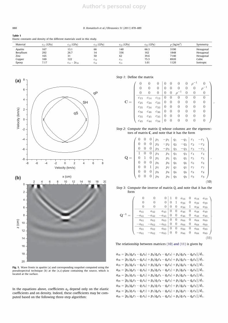
Fig. 1. Wave fronts in apatite (a) and corresponding snapshot computed using thepseudospectral technique (b) at the (x,z)-plane containing the source, which islocated at the surface.

880 D. Komatitsch et al. / Ultrasonics 51 (2011) 878–889


together with

;

where

d1 ¼ p9ðq6r8 � q8r6Þ þ p8ðq9r6 � q6r9Þ þ p6ðq8r9 � q9r8Þ;

d2 ¼ 2½p3ðq1r2 � q2r1Þ þ p2ðq3r1 � q1r3Þ þ p1ðq2r3 � q3r2Þ�:

Finally, the non-reflecting (i.e., absorbing) boundary conditionsarise from the following system of equations for the particlevelocities

a41 a42 a43

a61 a62 a63

a81 a82 a83

0B@

1CA

vx

vy

vz

0B@

1CAðnewÞ

¼ �12

b5

b7

b9

0B@

1CA;

together with the following system of equations for the stresses

a14 0 a16 0 a18 a19

0 a25 a26 0 a28 a29

0 0 a36 a37 a38 a39

0 0 a46 0 a48 a49

0 0 a66 0 a68 a69

0 0 a86 0 a88 a89

0BBBBBBBBBBB@

1CCCCCCCCCCCA

rxx

ryy

rzz

rxy

rxz

ryz

0BBBBBBBBBBB@

1CCCCCCCCCCCA

ðnewÞ

¼

b1

b2

b3

b5=2

b7=2

b9=2

0BBBBBBBBBBB@

1CCCCCCCCCCCA;

where

(a)

(b)

Fig. 2. Same as Fig. 1 for zinc.

(a)

(b)

Fig. 3. Same as Fig. 1 for copper.



b5

b7

b9

0B@

1CA ¼ �A

vx

vy

vz

0B@

1CAðoldÞ

þ Brzz

rxz

ryz

0B@

1CAðoldÞ

;

with A and B given in (9), while b1, b2 and b3 are given by (8).

3.2. The spectral-element method

In the spectral-element method (SEM), which is a continuousGalerkin approach, the strong form of the equations of motion(1) is first rewritten in a variational or weak formulation. Usingsuch a variational approach has the direct advantage that thefree-surface boundary condition at the surface of the model, whichsays that traction should be zero along the surface, is the natural

boundary condition of the technique. Thus, one does not need toimplement it explicitly, it is automatically enforced accurately. Be-cause of that, the propagation of surface waves and their interac-tion with the shape of the surface of laboratory models can becomputed in a very precise fashion [27]. This is true for geophysicalmodels as well, for which the effect of complex topography on bothsurface waves and body waves can be accurately predicted [28].

The SEM being a full waveform modeling technique, it can com-pute terms that are often neglected in approximate methods, forinstance the near-field terms [29]. Another advantage of that tech-nique is that, contrary to finite-difference methods for instance, itdoes not need to resort to a staggered numerical grid in which dif-ferent components of the strain tensor are defined at differentlocations; on the contrary, in the SEM all the components are de-fined at the same Gauss–Lobatto–Legendre grid point, and as a

0

4

8

12

16

20

24

28

32

36

40

y (c

m)

x (cm)

0

4

8

12

16

20

24

28

32

36

40

y (c

m)

x (cm)

0

4

8

12

16

20

24

28

32

36

40

y (c

m)

0 4 8 12 16 20 24 28 32 36 40 0 4 8 12 16 20 24 28 32 36 40

0 4 8 12 16 20 24 28 32 36 400 4 8 12 16 20 24 28 32 36 40

x (cm)

0

4

8

12

16

20

24

28

32

36

40

y (c

m)

x (cm)

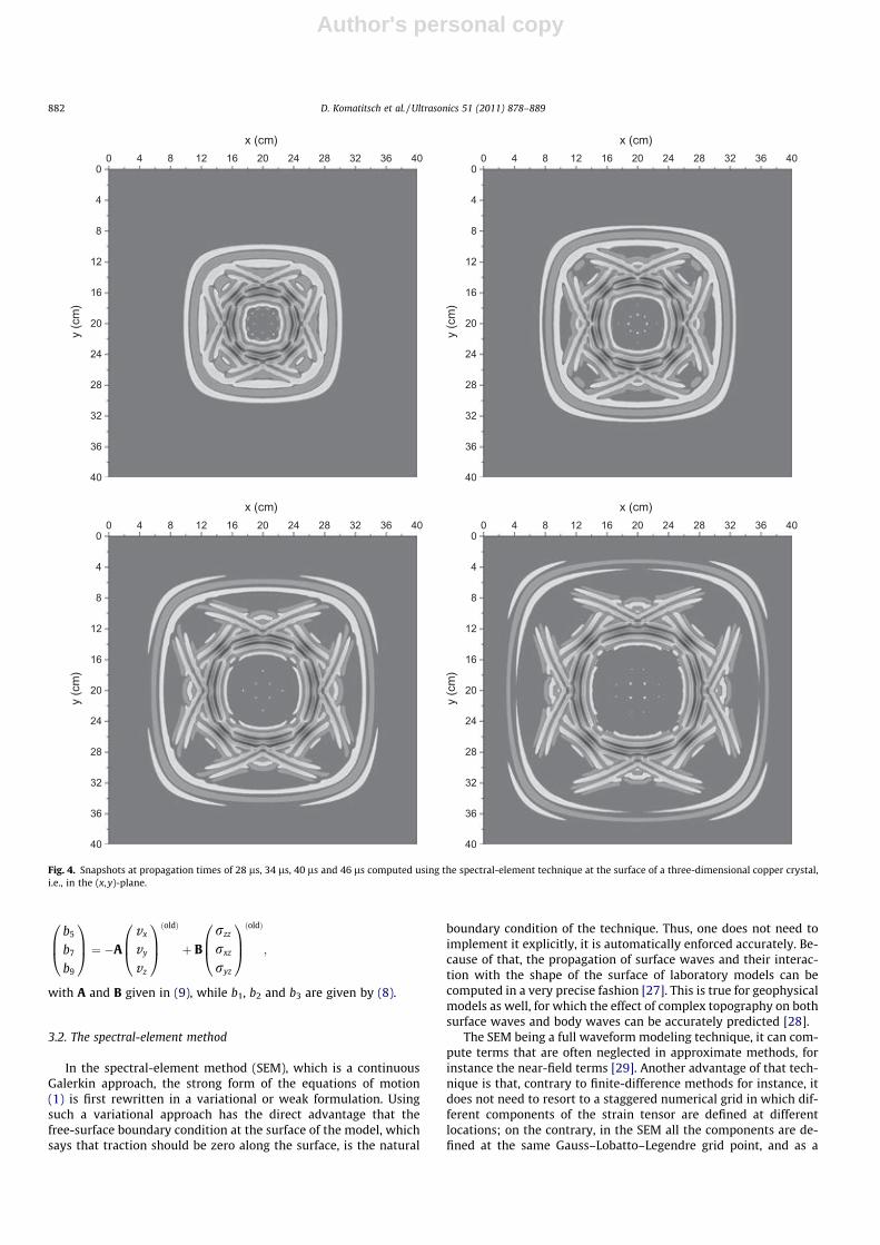
Fig. 4. Snapshots at propagation times of 28 ls, 34 ls, 40 ls and 46 ls computed using the spectral-element technique at the surface of a three-dimensional copper crystal,i.e., in the (x,y)-plane.



result the sum of all the strain terms required by Hooke’s law in thecase of general anisotropic media (2) can be performed withoutany additional interpolation. As a result, the SEM is very well sui-ted to studying elastic wave propagation in complex anisotropicmedia [30–32].

Another important property of the SEM is the fact that it can beparallelized efficiently to take advantage of the distributed struc-ture of modern supercomputers [33], and in particular on clustersof Graphics Processing Units (GPU) graphics cards [34–36], reach-ing speedup factors of more than an order of magnitude comparedto a reference serial implementation on a CPU core; this makes itcompare well in terms of performance to less flexible algorithmssuch as finite differences in the time domain (FDTD), which canalso be implemented efficiently on GPUs [37,38].

Writing the variational form of the elastic wave equation isaccomplished by dotting the strong (i.e., differential) form of the

equation with an arbitrary test vector w and integrating by partsover the region of interest:

ZXqw � €udXþ

ZX

$w : C : $udX

¼Z

Xw � f dXþ

ZCabs

w � tdC; ð12Þ

where f denotes the known external source force, t denotes thetraction vector, and X denotes the domain under study, whoseboundary C usually consists in two parts: a boundary Cf on whichfree-surface (i.e., traction-free) conditions are implemented, and anartificial boundary Cabs used to truncate semi-infinite domains andon which outgoing waves must be absorbed. In the integration bypart above, we have used the fact that the traction vanishes onthe free boundaries Cf of the domain and thus the related termsdoes not appear in the weak formulation because it is its naturalboundary condition. In order to absorb outgoing waves on the ficti-tious edges of the mesh, Convolution Perfectly Matched absorbingLayers (C-PML) are implemented, see e.g. [39–41]; however in thecase of elastic wave propagation in anisotropic crystals usually allthe edges of the crystal are either free (‘Neumann’ boundary condi-tion) or fixed/rigid with zero displacement (‘Dirichlet’ boundarycondition) because the crystal is of finite size and thus no absorbingconditions need to be implemented.

To implement the Legendre spectral element discretization ofthe variational problem (12), one first needs to create a mesh ofnel non-overlapping hexahedra Xe on the domain X, as in a classi-cal finite element method (FEM). These elements are subsequentlymapped to a reference cube K = [�1,1]3 using an invertible local

(a)

(b)

Fig. 5. Snapshots computed using the pseudospectral technique at the surface ofapatite, with the symmetry axis making an angle p/4 (a) and an angle p/2 (b) withthe surface.

tP tS

tR

10 20 30 40Time (µs)

0 50 -30

-25

-20

-15

-10

-5

0

5

10

Parti

cle

velo

city

(mm

/s)

(a)

tP tS tR

0 10 20 30 40 50 Time (µs)

0

0.5

1

1.5

2

Parti

cle

velo

city

(mm

/s)

(b)

Fig. 6. Analytical three-dimensional Green’s function (i.e., impulse response) forapatite (a) and beryllium (b) computed 15 cm below the source. Symbols tP and tR

denote the arrival time of qP and surface waves, respectively, while tS is the arrivaltime of SH and qSV modes.



mapping Fe : K! Xe, which enables one to go from the physicaldomain to the reference domain, and vice versa.

On the reference domain K, one introduces a set of local basisfunctions consisting of polynomials of degree N. On each element

Xe, mapped to the reference domain K, one then defines a set ofnodes and chooses the polynomial approximation ue

N and weN of u

and w to be the Lagrange interpolant at this set of nodes. Thesenodes ni 2 [�1,1], i 2 0, . . . ,N, are the Gauss–Lobatto–Legendre(GLL) points which are the (N + 1) roots of

ð1� n2ÞP0NðnÞ ¼ 0; ð13Þ

where P0NðnÞ is the derivative of the Legendre polynomial of degreeN. On the reference domain K, the restriction of a given function uN

to the element Xe can be expressed as

ueNðn;g; cÞ ¼

XN

p¼0

XN

q¼0

XN

r¼0

ueNðnp;gq; crÞhpðnÞhqðgÞhrðcÞ; ð14Þ

where hp(n) denotes the pth 1-D Lagrange interpolant at the (N + 1)GLL points ni introduced above, which is by definition the uniquepolynomial of degree N that is equal to one at n = np and to zeroat all other points n = nq for which q – p. From this definition, oneobtains the crucial property

hpðnqÞ ¼ dpq; ð15Þ

which will lead to a perfectly diagonal mass matrix.After introducing the piecewise-polynomial approximation

(14), the integrals in (12) can be approximated at the element levelusing the GLL integration rule:Z

XuNwN dX ¼

Xnel

e¼1

ZXe

ueNwe

N dX

’Xnel

e¼1

XN

i¼0

xi

XN

j¼0

xj

�XN

k¼0

xkJeðni;gj; ckÞueNðni;gj; ckÞwe

Nðni;gj; ckÞ: ð16Þ

-1

-0.5

0

0.5

1

20 25 30 35 40 45 50 20 25 30 35 40 45 50

Parti

cle

velo

city

Time (µs)Time (µs)

Time (µs)

AnalyticalSpectral elements

-1

-0.5

0

0.5

1

0 10 20 30 40 50 0 10 20 30 40 50

Parti

cle

velo

city

Parti

cle

velo

city

Parti

cle

velo

city

Time (µs)

AnalyticalSpectral elements1,0

0,5

0,0

-0,5

-1,0

1,0

0,5

0,0

-0,5

-1,0

(a)

(b)

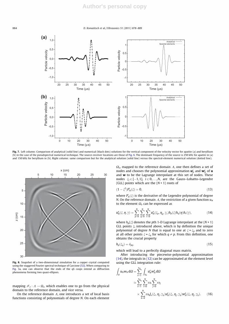
Fig. 7. Left column: Comparison of analytical (solid line) and numerical (black dots) solutions for the vertical component of the velocity vector for apatite (a) and beryllium(b) in the case of the pseudspectral numerical technique. The source-receiver locations are those of Fig. 6. The dominant frequency of the source is 250 kHz for apatite in (a)and 150 kHz for beryllium in (b). Right column: same comparison but for the analytical solution (solid line) versus the spectral-element numerical solution (dotted line).

x (cm)

z (c

m)

Fig. 8. Snapshot of a two-dimensional simulation for a copper crystal computedusing the staggered Fourier spectral technique of Carcione [52]. When comparing toFig. 3a, one can observe that the ends of the qS cusps extend as diffractionphenomena forming two quasi-ellipses.



The weights xi > 0 are independent of the element and are deter-mined numerically [42], and Je is the Jacobian associated with themapping Fe from the element Xe to the reference domain K.

Gradients are first computed in the reference domain K:

@nueNðn;g; cÞ ¼

XN

p¼0

XN

q¼0

XN

r¼0

ueNðnp;gq; crÞh

0pðnÞhqðgÞhrðcÞ;

@gueNðn;g; cÞ ¼

XN

p¼0

XN

q¼0

XN

r¼0

ueNðnp;gq; crÞhpðnÞh0qðgÞhrðcÞ;

@cueNðn;g; cÞ ¼

XN

p¼0

XN

q¼0

XN

r¼0

ueNðnp;gq; crÞhpðnÞhqðgÞh0rðcÞ;

ð17Þ

where h0 denotes the derivative of the 1-D Lagrange interpolant.One subsequently uses the chain rule to compute the derivativesin the physical domain, i.e.,

@x ¼ nx@n þ gx@g þ cx@c;

@y ¼ ny@n þ gy@g þ cy@c;

@z ¼ nz@n þ gz@g þ cz@c;

ð18Þ

where the components of the Jacobian matrix, nx, ny, nz etc. are com-puted based upon the mapping Fe.

The effects of anisotropy in (12) are included in the termRX $w : C : $udX, which can be rewritten as

RX rðuNÞ : $wNdX.

Written out explicitly, the integrand is

rðuNÞ : $wN ¼ rij@jwi: ð19Þ

In the fully anisotropic 3-D case, using the definitioneij = (@iuj + @jui)/2, Hooke’s law (2), when injected in (19) to obtainthe developed expression of rðuNÞ : $wN , gives a sum of terms ofthe form cab@aub@cwd, with cab the components of the reducedstiffness matrix in (2). Each of these terms, integrated over an ele-ment Xe, is easily computed by substituting the expansion of thefields (14), computing gradients using (17) and the chain rule(18), and using the GLL integration rule (16).

After this spatial discretization with spectral elements, impos-ing that (12) holds for any test vector wN, as in a classical FEM,we have to solve an ordinary differential equation in time. Denot-ing by �u the global vector of unknown displacement in the med-ium, we can rewrite Eq. (12) in matrix form as

M€�uþ K�u ¼ �f; ð20Þ

where M is called the mass matrix, K the stiffness matrix, and �f thesource term. A very important property of the Legendre SEM usedhere from an implementation point of view, which allows for adrastic reduction in the complexity and the cost of the algorithm,is the fact that the mass matrix M is diagonal; this stems fromthe choice of Lagrange interpolants at the GLL points in conjunctionwith the GLL integration rule, which results in (15). This constitutesa significant difference compared to a classical FEM and to theChebyshev SEM of Patera [15] and of e.g. Priolo et al.[43]. As a result,fully explicit time evolution schemes can be used.

Time discretization of the second-order ordinary differentialequation in time (20) is performed based on a classical explicitNewmark centered finite-difference scheme [44], which is sec-ond-order accurate and conditionally stable. We assume zero ini-tial conditions for the displacement and velocity fields, i.e., themedium is initially at rest. Higher-order time schemes can be usedif needed, for instance fourth-order Runge-Kutta or symplecticschemes [45,46]; this can be useful in particular for simulationscomprising a very large number of time steps, for which the factthat the spatial SEM discretisation is of high order while the timediscretisation is only second order implies that overall accuracyis significantly reduced because of the time scheme.

4. Numerical simulations

We consider the materials whose properties are given in Table1, and which are dissimilar: apatite, beryllium and zinc have hex-agonal symmetry and copper has cubic symmetry, with c22 = c11,while epoxy is isotropic.

The pseudospectral method uses a mesh composed of 81 gridpoints along the three Cartesian directions, with a constant gridspacing of 2.5 mm along the x- and y-directions and a total meshsize of 20 cm in the z-direction with varying grid spacing. The sur-face of the sample is the (x,y,z = 0)-plane. The source is a verticalforce located at the surface and has the time history

hðtÞ ¼ cos½2pðt � t0Þf0� exp �2ðt � t0Þ2f 20

h i; ð21Þ

where f0 is the dominant frequency and t0 = 3/(2f0) + 5.10�6 s is aonset delay time that we use in order to ensure zero initial condi-tions. The time step of the Runge-Kutta algorithm is 0.05 ls for apa-tite and 0.1 ls for zinc and copper. Figs. 1–3 show the wavefronts(energy velocities) in an unbounded medium and snapshots in the(x,z)-plane for apatite, zinc and copper. The dominant frequencies

(a)

(b)

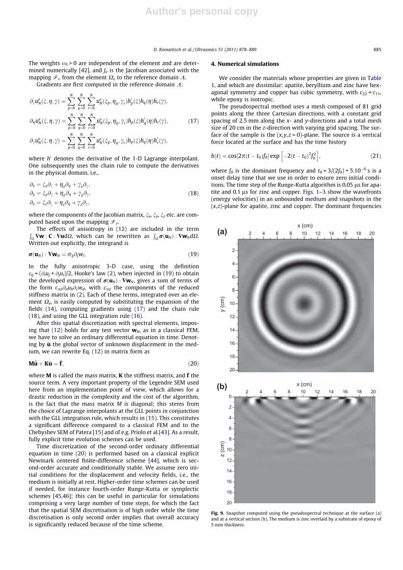
Fig. 9. Snapshot computed using the pseudospectral technique at the surface (a)and at a vertical section (b). The medium is zinc overlaid by a substrate of epoxy of5 mm thickness.



of the source are 250 kHz, 150 kHz and 200 kHz, with total propaga-tion times of 25 ls, 50 ls and 40 ls, respectively.

The Rayleigh wave can be observed at the surface, and the qPand qS waves in the interior of the medium. Fig. 4 showsspectral-element snapshots at different propagation times at thesurface of copper, i.e., in the (001)-plane in terms of Miller indices,where the Rayleigh wavefront can be seen [47].

The mesh contains a total of 90 � 90 � 90 spectral elements andwe use polynomial basis functions of degree N = 4. The total size ofthe mesh is 40 cm � 40 cm � 40 cm and we use a time step of0.03 ls. Apatite and zinc are azimuthally isotropic in this surfaceand therefore the wavefront is isotropic. Snapshots for the pseudo-spectral method of the wave field at the surface of apatite, with thesample rotated by an angle of p/4 and then an angle of p/2 withrespect to the surface are displayed in Fig. 5. The surfaces are the(101)- and (100)-planes in terms of Miller indices. In this case,the anisotropy of the Rayleigh wave can clearly be observed.

The analytical solution [48] for the three-dimensional Green’sfunction (i.e., the impulse response) for a surface source and a

receiver located along a vertical line below the source, in the inte-rior of the medium, is represented in Fig. 6.

For completeness the analytical expression to compute it is gi-ven in Appendix A. It corresponds to the Green function computed15 cm below the surface for apatite and then for beryllium. The P-and S-wave velocities of beryllium are almost twice that of othermetals, i.e., 13,484 m/s and 9363 m/s along the symmetry axis,respectively. These high velocities allow us to use a larger gridspacing of 4.4 mm in the x- and y-directions for the pseudospectraltechnique and a total mesh size of 35 cm in the z-direction, keepingthe same time step as that used for apatite, i.e., 0.05 ls; using asmaller grid allows us to save in terms of computational cost. Val-idation tests for both modeling algorithms versus the analyticalsolution convolved with the source time history (21) for apatiteand beryllium are shown in Fig. 7. The fit obtained is excellentfor both techniques.

In the case of the spectral-element method, the mesh contains atotal of 60 � 60 � 60 spectral elements and we use polynomialbasis functions of degree N = 4. The total size of the mesh is

20 cm

5 cm Zinc

Epoxy

(a)

(b) (c)

15 c

m

*

xy

z

Fig. 10. Model made of epoxy and zinc (a) and corresponding surface waves (b) and snapshot computed using the pseudospectral technique at a vertical section (c).



40 cm � 40 cm � 40 cm in the case of apatite and 60 cm �60 cm � 60 cm in the case of beryllium, and we use a time step of0.03 ls.

The practical applications of numerical modeling are numerous.One of them is to use it as a research tool to numerically investi-gate the complex behavior of waves propagating in crystals whenan analytical or closed form solution is not available. Recently, Des-champs and his collaborators [49–51] showed that the cuspidal tri-angles of the qS wave extend beyond the edges or vertices of thecuspidal triangles, and that this phenomenon can be explainedby inhomogeneous plane waves. In order to show this, we performa simulation using a two-dimensional qP–qS modeling algorithmbased on the staggered Fourier method to compute the spatialderivatives [52]. The mesh has 120 � 120 grid points with aconstant grid spacing of 2.5 mm. A vertical force with a dominant

frequency of 200 kHz is applied at its center. Fig. 8 shows a snap-shot at a time of 36 ls for a copper crystal; the qP and qS wavescan be seen (outer and inner wavefronts, respectively). When com-paring to Fig. 3a, one can observe that the ends of the qS cusps ex-tend as diffraction phenomena forming two quasi-ellipses.

Because the simulation is two dimensional and the source isplaced in the center of the model, it contains no surface waves,only body waves. This explains why this snapshot looks differentfrom the snapshots of Fig. 4, which are dominated by surfacewaves. Indeed, as the simulation illustrated in Fig. 4 is threedimensional with the source located exactly at the surface, Fig. 4thus not only has body waves as in Fig. 3a, but also surface wavessuperimposed and dominant.

The proposed modeling algorithms can handle heterogeneousmedia, therefore numerical simulations can be performed in casesfor which there is no known analytical solution. In the nextsimulation we consider a zinc sample coated with a substrate ofepoxy of 5 mm thickness. Epoxy is isotropic and has the elasticconstants given in Table 1. The simulation uses the same numericalparameters as those used to generate Fig. 2, but the vertical forcesource is located at a depth of 1 cm in the zinc crystal. In the snap-shots of Fig. 9, isotropic and dispersive Rayleigh wavefronts can beseen at the surface, and we notice that most of the energy is con-tained in the thin substrate.

The model shown in Fig. 10a is composed of a prism of epoxyembedded in zinc. The numerical parameters are unchanged andthe source is a combination of three directional forces applied atthe location indicated by a star in the model. Figs. 10b and c showsnapshots at the surface and at vertical section at a time of 55 ls,respectively. Most of the energy is trapped in the epoxy prism.

Fig. 11 shows snapshots at a time of 50 ls at the same planesbut replacing the epoxy prism with a copper prism. The impedancecontrast between the two media is weaker and therefore energytrapping is much reduced.

5. Conclusions

The two numerical modeling methods compute the full wavefield and have spectral accuracy. At each grid point these methodsallow us to model an anisotropic medium of arbitrary crystal sym-metry, i.,e., a triclinic medium or a medium of lower symmetrywhose symmetry axes can be rotated by any angle. We have shownnumerical examples for media of hexagonal or cubic symmetry, forwhich we obtained time histories and snapshots at the surface andat vertical sections. The wavefronts have been compared with theray surfaces (energy or group velocities) obtained based on aplane-wave analysis. The modeling algorithms have been success-fully tested against the analytical solution for a point force sourcelocated at the surface of a crystal and a receiver located in the inte-rior of the medium. We have shown how these modeling tools canbe used to simulate phenomena predicted by plane-wave analyses,as the continuation of the cuspidal triangles of the qS wave in cubiccrystals. Moreover, we have simulated wave propagation in thepresence of a free surface in cases where there is no analytical solu-tion for models composed of media of dissimilar crystal symmetryand with contrasting elastic properties.

Acknowledgements

The authors thank Arthur G. Every for fruitful discussion.Some of the calculations were performed on an SGI cluster at

Centre Informatique National de l’Enseignement Suprieur (CINES)in Montpellier, France. This material is based in part upon researchsupported by European FP6 Marie Curie International Reintegra-tion Grant MIRG-CT-2005-017461.

(a)

(b)

Fig. 11. Surface waves (a) and snapshot computed using the pseudospectraltechnique at a vertical section (b) corresponding to the model shown in Fig. 10a,replacing epoxy with copper.



Appendix A. Analytical solution for transversely isotropic media

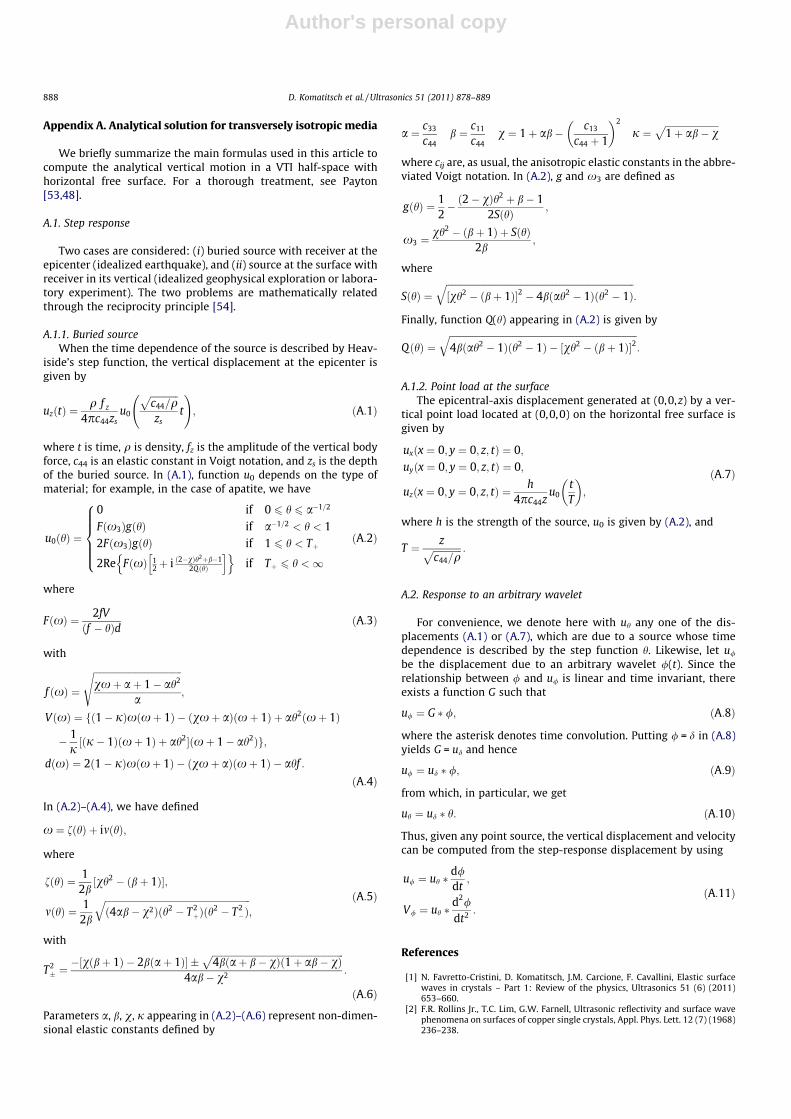
We briefly summarize the main formulas used in this article tocompute the analytical vertical motion in a VTI half-space withhorizontal free surface. For a thorough treatment, see Payton[53,48].

A.1. Step response

Two cases are considered: (i) buried source with receiver at theepicenter (idealized earthquake), and (ii) source at the surface withreceiver in its vertical (idealized geophysical exploration or labora-tory experiment). The two problems are mathematically relatedthrough the reciprocity principle [54].

A.1.1. Buried sourceWhen the time dependence of the source is described by Heav-

iside’s step function, the vertical displacement at the epicenter isgiven by

uzðtÞ ¼q f z

4pc44zsu0

ffiffiffiffiffiffiffiffiffiffiffiffic44=q

pzs

t

!; ðA:1Þ

where t is time, q is density, fz is the amplitude of the vertical bodyforce, c44 is an elastic constant in Voigt notation, and zs is the depthof the buried source. In (A.1), function u0 depends on the type ofmaterial; for example, in the case of apatite, we have

u0ðhÞ ¼

0 if 0 6 h 6 a�1=2

Fðx3ÞgðhÞ if a�1=2 < h < 12Fðx3ÞgðhÞ if 1 6 h < Tþ

2Re FðxÞ 12þ i ð2�vÞh

2þb�12QðhÞ

h in oif Tþ 6 h <1

8>>>><>>>>:

ðA:2Þ

where

FðxÞ ¼ 2fVðf � hÞd ðA:3Þ

with

f ðxÞ ¼

ffiffiffiffiffiffiffiffiffiffiffiffiffiffiffiffiffiffiffiffiffiffiffiffiffiffiffiffiffiffiffiffiffiffiffiffiffiffivxþ aþ 1� ah2

a

s;

VðxÞ ¼ fð1� jÞxðxþ 1Þ � ðvxþ aÞðxþ 1Þ þ ah2ðxþ 1Þ

� 1j½ðj� 1Þðxþ 1Þ þ ah2�ðxþ 1� ah2Þg;

dðxÞ ¼ 2ð1� jÞxðxþ 1Þ � ðvxþ aÞðxþ 1Þ � ahf :

ðA:4Þ

In (A.2)–(A.4), we have defined

x ¼ fðhÞ þ imðhÞ;

where

fðhÞ ¼ 12b½vh2 � ðbþ 1Þ�;

mðhÞ ¼ 12b

ffiffiffiffiffiffiffiffiffiffiffiffiffiffiffiffiffiffiffiffiffiffiffiffiffiffiffiffiffiffiffiffiffiffiffiffiffiffiffiffiffiffiffiffiffiffiffiffiffiffiffiffiffiffiffiffiffiffiffiffiffiffiffið4ab� v2Þðh2 � T2

þÞðh2 � T2

�Þq

;

ðA:5Þ

with

T2� ¼�½vðbþ 1Þ � 2bðaþ 1Þ� �

ffiffiffiffiffiffiffiffiffiffiffiffiffiffiffiffiffiffiffiffiffiffiffiffiffiffiffiffiffiffiffiffiffiffiffiffiffiffiffiffiffiffiffiffiffiffiffiffiffiffiffiffiffiffiffiffiffi4bðaþ b� vÞð1þ ab� vÞ

p4ab� v2 :

ðA:6Þ

Parameters a, b, v, j appearing in (A.2)–(A.6) represent non-dimen-sional elastic constants defined by

a ¼ c33

c44b ¼ c11

c44v ¼ 1þ ab� c13

c44 þ 1

� �2

j ¼ffiffiffiffiffiffiffiffiffiffiffiffiffiffiffiffiffiffiffiffiffiffiffi1þ ab� v

pwhere cij are, as usual, the anisotropic elastic constants in the abbre-viated Voigt notation. In (A.2), g and x3 are defined as

gðhÞ ¼ 12� ð2� vÞh2 þ b� 1

2SðhÞ ;

x3 ¼vh2 � ðbþ 1Þ þ SðhÞ

2b;

where

SðhÞ ¼ffiffiffiffiffiffiffiffiffiffiffiffiffiffiffiffiffiffiffiffiffiffiffiffiffiffiffiffiffiffiffiffiffiffiffiffiffiffiffiffiffiffiffiffiffiffiffiffiffiffiffiffiffiffiffiffiffiffiffiffiffiffiffiffiffiffiffiffiffiffiffiffiffiffiffiffiffiffiffiffiffi½vh2 � ðbþ 1Þ�2 � 4bðah2 � 1Þðh2 � 1Þ

q:

Finally, function Q(h) appearing in (A.2) is given by

QðhÞ ¼ffiffiffiffiffiffiffiffiffiffiffiffiffiffiffiffiffiffiffiffiffiffiffiffiffiffiffiffiffiffiffiffiffiffiffiffiffiffiffiffiffiffiffiffiffiffiffiffiffiffiffiffiffiffiffiffiffiffiffiffiffiffiffiffiffiffiffiffiffiffiffiffiffiffiffiffiffiffiffiffiffi4bðah2 � 1Þðh2 � 1Þ � ½vh2 � ðbþ 1Þ�2

q:

A.1.2. Point load at the surfaceThe epicentral-axis displacement generated at (0,0,z) by a ver-

tical point load located at (0,0,0) on the horizontal free surface isgiven by

uxðx ¼ 0; y ¼ 0; z; tÞ ¼ 0;uyðx ¼ 0; y ¼ 0; z; tÞ ¼ 0;

uzðx ¼ 0; y ¼ 0; z; tÞ ¼ h4pc44z

u0tT

� �;

ðA:7Þ

where h is the strength of the source, u0 is given by (A.2), and

T ¼ zffiffiffiffiffiffiffiffiffiffiffiffic44=q

p :

A.2. Response to an arbitrary wavelet

For convenience, we denote here with uh any one of the dis-placements (A.1) or (A.7), which are due to a source whose timedependence is described by the step function h. Likewise, let u/

be the displacement due to an arbitrary wavelet /(t). Since therelationship between / and u/ is linear and time invariant, thereexists a function G such that

u/ ¼ G � /; ðA:8Þ

where the asterisk denotes time convolution. Putting / = d in (A.8)yields G = ud and hence

u/ ¼ ud � /; ðA:9Þ

from which, in particular, we get

uh ¼ ud � h: ðA:10Þ

Thus, given any point source, the vertical displacement and velocitycan be computed from the step-response displacement by using

u/ ¼ uh �d/dt;

V/ ¼ uh �d2/

dt2 :

ðA:11Þ

References

[1] N. Favretto-Cristini, D. Komatitsch, J.M. Carcione, F. Cavallini, Elastic surfacewaves in crystals – Part 1: Review of the physics, Ultrasonics 51 (6) (2011)653–660.

[2] F.R. Rollins Jr., T.C. Lim, G.W. Farnell, Ultrasonic reflectivity and surface wavephenomena on surfaces of copper single crystals, Appl. Phys. Lett. 12 (7) (1968)236–238.



[3] F.R. Rollins Jr., Ultrasonic examination of liquid–solid boundaries using a right-angle reflector technique, J. Acoust. Soc. Am. 44 (2) (1968) 431–434.

[4] A.A. Kolomenskii, A.A. Maznev, Phonon-focusing effect with laser-generatedultrasonic surface waves, Phys. Rev. B 48 (19) (1993) 14502–14512.

[5] A.G. Every, K.Y. Kim, A.A. Maznev, Surface dynamic response functions ofanisotropic solids, Ultrasonics 36 (1998) 349–353.

[6] A.G. Every, M. Deschamps, Principal surface wave velocities in the point focusacoustic materials signature V(z) of an anisotropic solid, Ultrasonics 41 (2003)581–591.

[7] J.X. Dessa, G. Pascal, Combined traveltime and frequency-domain seismicwaveform inversion: a case study on multi-offset ultrasonic data, Geophys. J.Int. 154 (1) (2003) 117–133, doi:10.1046/j.1365-246X.2003.01956.x.

[8] A.N. Darinskii, M. Weihnacht, Acoustic waves in bounded anisotropic media:theorems, estimations, and computations, IEEE Trans. Ultrason. Ferroelectr.Freq. Control 52 (5) (2005) 792–801.

[9] K. Helbig, Foundations of anisotropy for exploration seismics, in: K. Helbig, S.Treitel (Eds.), Handbook of Geophysical Exploration, Section I: SeismicExploration, vol. 22, Pergamon, Oxford, England, 1994.

[10] S. Crampin, E.M. Chesnokov, R.G. Hipkin, Seismic anisotropy – the state of theart II, Geophys. J. Roy. Astron. Soc. 76 (1984) 1–16.

[11] L. Thomsen, Weak elastic anisotropy, Geophysics 51 (1986) 1954–1966.[12] J.M. Carcione, Wave Fields in Real Media: Theory and Numerical Simulation of

Wave Propagation in Anisotropic, Anelastic, Porous and ElectromagneticMedia, second ed., Elsevier Science, Amsterdam, The Netherlands, 2007.

[13] E. Tessmer, 3-D seismic modelling of general material anisotropy in thepresence of the free surface by a Chebyshev spectral method, Geophys. J. Int.121 (1995) 557–575.

[14] D. Komatitsch, F. Coutel, P. Mora, Tensorial formulation of the wave equationfor modelling curved interfaces, Geophys. J. Int. 127 (1) (1996) 156–168,doi:10.1111/j.1365-246X.1996.tb01541.x.

[15] A.T. Patera, A spectral element method for fluid dynamics: laminar flow in achannel expansion, J. Comput. Phys. 54 (1984) 468–488.

[16] D. Komatitsch, J.P. Vilotte, The spectral-element method: an efficient tool tosimulate the seismic response of 2D and 3D geological structures, Bull.Seismol. Soc. Am. 88 (2) (1998) 368–392.

[17] R. Vai, J.M. Castillo-Covarrubias, F.J. Sánchez-Sesma, D. Komatitsch, J.P. Vilotte,Elastic wave propagation in an irregularly layered medium, Soil Dyn.Earthquake Eng. 18 (1) (1999) 11–18, doi:10.1016/S0267-7261(98)00027-X.

[18] G. Cohen, Higher-Order Numerical Methods for Transient Wave Equations,Springer-Verlag, Berlin, Germany, 2002.

[19] M.O. Deville, P.F. Fischer, E.H. Mund, High-Order Methods for IncompressibleFluid Flow, Cambridge University Press, Cambridge, United Kingdom, 2002.

[20] J. Tromp, D. Komatitsch, Q. Liu, Spectral-element and adjoint methods inseismology, Communications in Computational Physics 3 (1) (2008) 1–32.

[21] J.M. Carcione, D. Kosloff, R. Kosloff, Wave propagation simulation in an elasticanisotropic (transversely isotropic) solid, Quart. J. Mech. Appl. Math. 41 (3)(1988) 319–345.

[22] J.M. Carcione, D. Kosloff, A. Behle, G. Seriani, A spectral scheme for wavepropagation simulation in 3-D elastic-anisotropic media, Geophysics 57 (12)(1992) 1593–1607.

[23] D. Kosloff, D. Kessler, A.Q. Filho, E. Tessmer, A. Behle, R. Strahilevitz, Solution ofthe equations of dynamic elasticity by a Chebychev spectral method,Geophysics 55 (1990) 734–748, doi:10.1190/1.1442885.

[24] J.M. Carcione, F. Poletto, D. Gei, 3-D wave simulation in anelastic media usingthe Kelvin-Voigt constitutive equation, J. Comput. Phys. 196 (2004) 282–297.

[25] B. Lombard, J. Piraux, Numerical treatment of two-dimensional interfaces foracoustic and elastic waves, J. Comput. Phys. 195 (1) (2004) 90–116,doi:10.1016/j.jcp.2003.09.024.

[26] P. Moczo, J. Robertsson, L. Eisner, The finite-difference time-domain methodfor modeling of seismic wave propagation, in: R.-S. Wu, V. Maupin (Eds.),Advances in Wave Propagation in Heterogeneous Media, Advances inGeophysics, vol. 48, Elsevier-Academic Press, London, UK, 2007, pp. 421–516. Chapter 8.

[27] K. van Wijk, D. Komatitsch, J.A. Scales, J. Tromp, Analysis of strong scattering atthe micro-scale, J. Acoust. Soc. Am. 115 (3) (2004) 1006–1011, doi:10.1121/1.1647480.

[28] S.J. Lee, H.W. Chen, Q. Liu, D. Komatitsch, B.S. Huang, J. Tromp, Three-dimensional simulations of seismic wave propagation in the Taipei basin withrealistic topography based upon the spectral-element method, Bull. Seismol.Soc. Am. 98 (1) (2008) 253–264, doi:10.1785/0120070033.

[29] N. Favier, S. Chevrot, D. Komatitsch, Near-field influences on shear wavesplitting and traveltime sensitivity kernels, Geophys. J. Int. 156 (3) (2004) 467–482, doi:10.1111/j.1365-246X.2004.02178.x.

[30] G. Seriani, E. Priolo, A. Pregarz, Modelling waves in anisotropic media by aspectral element method, in: G. Cohen (Ed.), Proceedings of the ThirdInternational Conference on Mathematical and Numerical Aspects of WavePropagation, SIAM, Philadephia, PA, 1995, pp. 289–298.

[31] D. Komatitsch, C. Barnes, J. Tromp, Simulation of anisotropic wave propagationbased upon a spectral element method, Geophysics 65 (4) (2000) 1251–1260,doi:10.1190/1.1444816.

[32] S. Chevrot, N. Favier, D. Komatitsch, Shear wave splitting in three-dimensionalanisotropic media, Geophys. J. Int. 159 (2) (2004) 711–720, doi:10.1111/j.1365-246X.2004.02432.x.

[33] D. Komatitsch, L.P. Vinnik, S. Chevrot, SHdiff/SVdiff splitting in an isotropicearth, J. Geophys. Res. 115 (B7) (2010) B07312, doi:10.1029/2009JB006795.

[34] D. Komatitsch, D. Michéa, G. Erlebacher, Porting a high-order finite-elementearthquake modeling application to NVIDIA graphics cards using CUDA, J.Parallel Distrib. Comput. 69 (5) (2009) 451–460, doi:10.1016/j.jpdc.2009.01.006.

[35] D. Komatitsch, G. Erlebacher, D. Göddeke, D. Michéa, High-order finite-element seismic wave propagation modeling with MPI on a large GPU cluster,J. Comput. Phys. 229 (20) (2010) 7692–7714, doi:10.1016/j.jcp.2010.06.024.

[36] D. Komatitsch, Fluid-solid coupling on a cluster of GPU graphics cards forseismic wave propagation, Comptes Rendus de l’Académie des Sciences –Mécanique 339 (2011) 125–135.

[37] P. Micikevicius, 3D finite-difference computation on GPUs using CUDA, in:GPGPU-2: Proceedings of the 2nd Workshop on General Purpose Processing onGraphics Processing Units, Washington, DC, USA, 2009, pp. 79–84.doi:10.1145/1513895.1513905.

[38] D. Michéa, D. Komatitsch, Accelerating a 3D finite-difference wavepropagation code using GPU graphics cards, Geophys. J. Int. 182 (1) (2010)389–402, doi:10.1111/j.1365-246X.2010.04616.x.

[39] D. Komatitsch, R. Martin, An unsplit convolutional perfectly matched layerimproved at grazing incidence for the seismic wave equation, Geophysics 72(5) (2007) SM155–SM167, doi:10.1190/1.2757586.

[40] R. Martin, D. Komatitsch, S.D. Gedney, A variational formulation of a stabilizedunsplit convolutional perfectly matched layer for the isotropic or anisotropicseismic wave equation, Comput. Model. Eng. Sci. 37 (3) (2008) 274–304.

[41] R. Martin, D. Komatitsch, A. Ezziani, An unsplit convolutional perfectlymatched layer improved at grazing incidence for seismic wave equation inporoelastic media, Geophysics 73 (4) (2008) T51–T61, doi:10.1190/1.2939484.

[42] C. Canuto, M.Y. Hussaini, A. Quarteroni, T.A. Zang, Spectral Methods in FluidDynamics, Springer-Verlag, New-York, USA, 1988.

[43] E. Priolo, J.M. Carcione, G. Seriani, Numerical simulation of interface waves byhigh-order spectral modeling techniques, J. Acoust. Soc. Am. 95 (2) (1994)681–693.

[44] T.J.R. Hughes, The Finite Element Method, Linear Static and Dynamic FiniteElement Analysis, Prentice-Hall International, Englewood Cliffs, New Jersey,USA, 1987.

[45] N. Tarnow, J.C. Simo, How to render second-order accurate time-steppingalgorithms fourth-order accurate while retaining the stability andconservation properties, Comput. Meth. Appl. Mech. Eng. 115 (1994) 233–252.

[46] T. Nissen-Meyer, A. Fournier, F.A. Dahlen, A 2-D spectral-element method forcomputing spherical-earth seismograms – II. Waves in solid-fluid media,Geophys. J. Int. 174 (2008) 873–888, doi:10.1111/j.1365-246X.2008.03813.x.

[47] A. Maznev, A.M. Lomonosov, P. Hess, A.A. Kolomenskii, Anisotropic effects insurface acoustic wave propagation from a point source in a crystal, Euro. Phys.J. B 35 (2003) 429–439.

[48] R.G. Payton, Elastic Wave Propagation in Transversely Isotropic Media,Martinus Nijhoff, The Hague, The Netherlands, 1983.

[49] O. Poncelet, M. Deschamps, A. Every, B. Audoin, Extension to cuspidal edges ofwave surfaces of anisotropic solids: treatment of near cusp behavior, Rev. Prog.Quant. Nondestruct. Eval. 20 (2001) 51–58.

[50] M. Deschamps, O. Poncelet, Inhomogeneous plane wave and the mostenergetic complex ray, Ultrasonics 40 (2002) 293–296.

[51] M. Deschamps, G. Huet, Complex surface rays associated with inhomogeneousskimming and Rayleigh waves, Int. J. Nonlinear Mech. 44 (2009) 469–477.

[52] J.M. Carcione, Staggered mesh for the anisotropic and viscoelastic waveequation, Geophysics 64 (1999) 1863–1866.

[53] R.G. Payton, Epicenter and epicentral-axis motion of a transversely isotropicelastic half-space, SIAM J. Appl. Math. 40 (1981) 373–389.

[54] A. Ben-Menahem, S.J. Singh, Seismic Waves and Sources, Springer-Verlag, NewYork, 1981.


author's personal copy - luca baradello · author's personal copy where u denotes the...

Documents