author's personal copy - core · author's personal copy veri cation of the relationship...

This article appeared in a journal published by Elsevier. The attachedcopy is furnished to the author for internal non-commercial researchand education use, including for instruction at the authors institution

and sharing with colleagues.

Other uses, including reproduction and distribution, or selling orlicensing copies, or posting to personal, institutional or third party

websites are prohibited.

In most cases authors are permitted to post their version of thearticle (e.g. in Word or Tex form) to their personal website orinstitutional repository. Authors requiring further information

regarding Elsevier’s archiving and manuscript policies areencouraged to visit:

http://www.elsevier.com/copyright

http://www.elsevier.com/copyright

Author's personal copy

Diatom distribution in southeastern Pacific surface sediments and their relationshipto modern environmental variables

Oliver Esper ⁎, Rainer Gersonde, Nicole KadagiesAlfred-Wegener-Institute for Polar and Marine Research, Columbusstrasse, D-27568 Bremerhaven, Germany

a b s t r a c ta r t i c l e i n f o

Article history:Received 24 June 2009Received in revised form 23 November 2009Accepted 6 December 2009Available online 16 December 2009

Keywords:DiatomsMarine sedimentsAmundsen SeaBellingshausen SeaAntarctic Circumpolar CurrentCanonical redundancy analysis

The quantitative analysis of diatom assemblages preserved in 52 samples from the Bellingshausen and theAmundsen Seas provides the first comprehensive view on the distribution of diatoms in surface sediments ofthe eastern and central Pacific sector of the Southern Ocean. On a latitudinal transect along 120°W, diatomvalve accumulation rates (AR) reachmaximum values (8–10×108 valves m−2 yr−1) in a zone extending overca. 900 kmbetween theAntarctic Polar Front and themaximumaveragewinter sea ice extent and exceed thoseARs obtained from an eastern transect along 90°W by one order of magnitude. Lowest diatom concentrations(1–3×106 valves g−1) were encountered in sediments of the Sea Ice Zone, affected by winter and summer seaice. The accumulation rate pattern of themost abundant diatom Fragilariopsis kerguelensis (N50% abundance in47 samples) mirrors the pattern of the total diatom valve AR and the biogenic silica (BSi) AR, makingF. kerguelensis themajor contributor to the BSi preserved at the seafloor. Relative abundances of diatom speciesand species groups were statistically compared with a selection of environmental variables, such as the meansummer sea surface temperature and salinity,mean annual surface nutrient concentration (nitrate, phosphate,silicon), mean annual water column stratification, mixed layer depth in summer, and mean summer andwinter sea ice concentrations. Polynomial canonical redundancy analysis (RDA) revealed the biogeographicdistribution of diatom species had the strongest relationship with summer sea surface temperature (SSST) outof the nine tested environmental variables. This relationship accounted for 69.6% of the total variance of thediatom distribution, with 29.7% explained by the first gradient (significantly correlated to SSST withr2=0.941) and 15.6% explained by the second gradient (correlated to both summer and winter sea ice andsilicon concentration). Azpeitia tabularis, Hemidiscus cuneiformis and Roperia tesselata were associated withwarmer water conditions (N4 °C), whereas Fragilariopsis curta, F. separanda, F. rhombica and Thalassiosiragracilis were correlated with cold SSST (b1.5 °C). Under the second gradient relationship, Actinocyclusactinochilus and F. curtawere themost important diatoms representative of the diatom distribution in relationto the observed mean summer and winter sea ice concentrations.Confirming these environmental relationships is crucial for the development of reference data sets used inquantitative estimations of palaeoclimatic and palaeoceanographic conditions with statistical methods. Thisnew data set represents the first modernised treatment of diatom remains from the SE Pacific Ocean andgenerally supports the use of a circum-polar database for the determination of summer SST, sea ice andpotentially biogenic silica distribution of the Southern Ocean back into the Late Quaternary.

© 2010 Elsevier B.V. All rights reserved.

1. Introduction

The establishment of quantitative data sets on the diatom speciescomposition preserved in Southern Ocean surface sediments (Zielinskiand Gersonde, 1997; Pichon et al., 1998; Armand et al., 2005; Crosta et al.,2005; Romero et al., 2005) has allowed for the development of diatom-based transfer functions, which can be used to quantitatively reconstructpast Southern Ocean surface temperatures and sea ice concentrations(Pichon et al., 1987, 1992a,b, 1998; Zielinski et al., 1998; Crosta et al.,

1998a,b) and for the definition of species abundance patterns as atemplate for the estimation of past sea ice distribution (Gersonde andZielinski, 2000) and productivity regimes (Abelmann et al., 2006).Most ofourunderstandingof PleistoceneSouthernOcean sea surface temperature(SST) and sea ice conditions at specific time slices and glacial/interglacialvariability comes from diatom transfer function-based reconstructions(Crosta et al., 1998a,b, 2004; Zielinski et al., 1998; Bianchi and Gersonde,2002, 2004; Kunz-Pirrung et al., 2002; Gersonde et al., 2003a,b, 2005;ArmandandLeventer, 2003,2009).Although this approachhasessentiallymet with success, further studies are required to enhance our ability toreconstruct past Southern Ocean surface water conditions. This concernsprimarily the extension of the diatom reference data sets into the Pacificsector, as requested by Gersonde et al. (2005), combinedwith a statistical

Palaeogeography, Palaeoclimatology, Palaeoecology 287 (2010) 1–27

⁎ Corresponding author. Tel.: +49 471 4831 1077; fax: +49 471 4831 1923.E-mail address: [email protected] (O. Esper).

0031-0182/$ – see front matter © 2010 Elsevier B.V. All rights reserved.doi:10.1016/j.palaeo.2009.12.006

Contents lists available at ScienceDirect

Palaeogeography, Palaeoclimatology, Palaeoecology

j ourna l homepage: www.e lsev ie r.com/ locate /pa laeo


verification of the relationship between environmental variables and thedistribution of diatoms in modern sediments.

Although the Pacific sector of the Southern Ocean is the largest of theSouthern Ocean sectors, modern studies of the distribution of diatomspreserved in the sedimentary record relevant to this Pacific sector havebeen restricted to coastal environments and basins along the AntarcticPeninsula (Crosta et al., 1997; Zielinski and Gersonde, 1997), the Amund-sen Sea shelf (Kellogg and Kellogg, 1987) and the Ross Sea (Cunninghamand Leventer, 1998) rather than venturing into the Antarctic CircumpolarCurrent (ACC). South Pacific open-ocean assemblages have beenpresented by Kozlova (1966) and Donahue (1973) and recently from alimited number of sites by Armand et al. (2005), Crosta et al. (2005) andRomero et al. (2005). In contrast, detailed studies of diatoms from SouthPacific surfacewaters have been undertaken (e.g. Frenguelli and Orlando,1958; Kozlova, 1966; Hargraves, 1968; Hasle, 1969; Fenner et al., 1976;Hasle, 1976; Burckle et al., 1987; Savidge et al., 1995; de Baar et al., 1999).

In the absence of a reference data set for this area, palaeoenvironmentalreconstructionsbasedondiatomtransfer functions restontheassumptionand earlier dispersal observations (e.g. Discovery reports by Hart, 1934;Hendey, 1937; Baker, 1954) that diatom distributions are circumpolar incharacter, that is, that the distribution of the Atlantic and Indian sectorscan be extrapolated to the Pacific sector of the Southern Ocean. Byconfirming that the general zonal patternof diatomdistribution continuesthrough thePacific sector, palaeoceanographers couldconfidently supportthe pooling and application of reference data sets across the SouthernOcean for statistical analysis of core data from all sectors.

Here we present a comprehensive documentation of the diatomspecies distribution in the central and eastern Pacific sector of theSouthern Ocean. We examined 52 surface sediment samples collectedfromtwo transects around120°Wand90°Wbetween the central ACCandthe Antarctic near-shore coast (minimumwater depths of about 2000 m)(Fig. 1). Considering that the sea-floor diatom assemblage compositions

Fig. 1. Present-day surface oceanography in the Pacific sector of the Southern Ocean with the positions of the oceanic fronts (after Orsi et al., 1995; SAF: Subantarctic Front;APF: Antarctic Polar Front; PFZ: Polar Front Zone; sACCF: Southern ACC Front), the main sea surface currents (arrows; after Read et al., 1995; Nechaev et al., 1997; Smithet al., 1999), summer and winter sea ice extent (dashed lines; after Schweitzer, 1995), the bathymetry of the observed area (light grey: b 3000 m, medium grey: 3000–5000 m,dark grey: N 5000 m; taken from GEBCO: the General Bathymetric Chart of the Oceans) and the 52 sample positions.

Fig. 2. Environmental and physical variables characterising the (sub)surface water layer of the working area. Environmental variables are the mean sea surface summer temperature(TEMP; panel a) and the mean annual sea surface salinity (SAL; panel b), the mean annual dissolved nitrate concentration (NO3; panel c), the mean annual dissolved phosphateconcentration (PO4; panel d) and the mean annual dissolved silicon concentration (Si; panel e). Physical variables include the summer mixed layer depth (MLD; panel f) andthe mean annual stratification of the upper water column between 0 and 75 m expressed as Brunt–Väisälä-frequencies (N; panel g), the mean winter sea ice concentration (WSIC;panel h) and the mean summer sea ice concentration (SSIC; panel i).

2 O. Esper et al. / Palaeogeography, Palaeoclimatology, Palaeoecology 287 (2010) 1–27


3O. Esper et al. / Palaeogeography, Palaeoclimatology, Palaeoecology 287 (2010) 1–27


maybe biased by selective dissolution (Burckle and Cirilli, 1987), the stateof preservation of each samplewas carefully determined. Our study relieson diatom species percent abundance, but also considers diatom valveaccumulation rates. Comparison of diatom abundances with measuredenvironmental variables (SST, salinity, nutrient concentrations, watercolumn stability and sea ice concentration) relies on the results ofstatistical methods such as polynomial canonical redundancy analysis(polynomial RDA), to decipher the main environmental factors influenc-ing the diatom species and their abundance distributions. We alsocompare the diatom assemblages preserved in the surface sedimentswith the results from plankton studies accomplished in the Pacific sectorof the Southern Ocean. Such comparison is complicated by the fact thatplankton net studies generally present “snap shot”-information from aspecific season and the full range of diatoms including very weaklysilicified species while surface sediment samples integrate assemblagesdeposited over years to decades or thousands of years and are biasedtowards more strongly silicified species due to selective dissolution.Nevertheless, phytoplankton studies from the Pacific sector (Kozlova,1966;Hargraves, 1968;Hasle, 1969, 1976; Fenner et al., 1976;Kellogg andKellogg, 1987; Burckle et al., 1987; Savidge et al., 1995) provide additionalinformation on the autecological demands of the species preserved in thesediment record and can be used for a better understanding of

environmental processes that steer the distribution of diatom species inthe surface sediments.

2. Regional setting

The 52 studied surface sediment samples were recovered from theAmundsen and Bellingshausen Seas between 125°W–80°W and 75°S–50°S. The latitudinal coverage ranges from near-shore sites to the centralAntarctic Circumpolar Current (ACC). The study area can be subdividedinto four oceanographic zones, each characterised by specific hydro-graphic andnutrient regimes (Figs. 1 and2). The southernboundaryof thewarmer (SSST ca. 7–14 °C) Subantarctic Zone (SAZ) is the SubantarcticFront (SAF), marked by distinct changes in temperature (ca. 4 °C) andsalinity (ca. 0.22 PSU) (Lutjeharms and Valentine, 1984). The Polar FrontZone (PFZ) south of the SAF marks the northern limit of high nutrientregime typical of the Southern Ocean (Fig. 2). The PFZ is separated to itssouth by the Antarctic Polar Front (APF) from the Antarctic Zone (AZ),characterised by sea surface temperatures b4 °C and subsurface tem-peratures b2 °C. Highest Southern Ocean sea surface silicon concentra-tions occur in theAZ (Fig. 2). TheAZ isdivided fromnorth to south into thePermanent Open Ocean Zone (POOZ), the Seasonal Sea Ice Zone (SSIZ)and the Sea Ice Zone (SIZ) close to the Antarctic coast. The SIZ is affected

Fig. 3. Concentrations (valves/g) and preservation of the diatoms analysed in this study (preservation range: g=good, g–m=good–moderate, m=moderate, m–p=moderate–poor) in relation to the seafloor morphology in the Amundsen and Bellingshausen Seas (TMF: trough mouth fan; after Hillenbrand, 2000; Dowdeswell et al., 2006), and the bottomwater pathways after Reid (1986). Bathymetric isolines (500, 3000, 5000) indicate the water depth in meters.



by winter and summer sea ice. Embedded in the AZ is the southern ACCFront (sACCF), which marks the southern boundary of the ACC. Thelocation of this latter front is close to themaximumaveragewinter sea iceextent (WSI; Fig. 1) (e.g. Armand and Leventer, 2003). A westwardlydirected counter current occurs close to the Antarctic continent. Thecounter current´s bottomwater component is assumed to consist mainlyofWeddell SeaDeepWatergenerated in theScotia Sea (Reid, 1986;Orsi etal., 1999; Scheuer et al., 2006; Rodehacke et al., 2007) (Fig. 3). While thenorthern part of the study area is characterised by less stratified surfacewaterswith adeepermixed layer, the southern regionwithin the SSIZ andSIZ features stronger surface water stratification and a shallower mixedlayer during summer.

The sedimentary environment varies from the heterogeneous areaof the continental rise, characterised by sediment mounds, channelsand debris flows to more homogeneous sediments of the abyssal plainbelow the ACC (Hillenbrand, 2000; Dowdeswell et al., 2006) (Fig. 3).

3. Material and methods

3.1. Material

Fifty-two surface sediment samples (Fig. 1; Table 1) were collectedwith a multicorer during AWI R/V Polarstern cruises ANT-XI/3, ANT-XII/4 and ANT-XVIII/5a (Miller and Grobe, 1996; http://www.pangaea.de/

Table 1Station list and characteristics of the 52 analysed sediment samples.

Station a Latitude Longitude Waterdepth(m)

Sedimenttype b

Bulk sediment AR(g m−2 yr−1)c

BSi(%)c

BSi AR(mmolm−2 yr−1) c

Totaldiatomcounts

×106 Diatoms/gdry weight

Total diatom AR(×108 valvesm−2 yr−1)

Diatompreservation d

PS2546-1 72°03.12´S 120°55.77´W 2384 fbsm 56 0.5 m–pPS2547-2 71°09.05´S 119°55.14´W 2092 fbsm 145 2.4 mPS2548-2 70°47.38´S 119°30.43´W 2642 fbm 71 1.4 mPS2550-2 69°51.53´S 118°13.00´W 3108 fbm 97 2.8 m–pPS2657-1 51°21.90´S 82°13.20´W 4367 fbdm 548 17.5 mPS2659-2* 50°44.94´S 85°41.28´W 4579 dbfm 2.5 10.2 3.9 599 38.4 0.97 mPS2661-4* 51°24.54´S 89°20.70´W 4728 dbfm 2.6 9.5 3.7 520 41.5 1.08 mPS2663-4* 53°17.22´S 89°32.82´W 4972 dm 1.9 16.1 4.7 486 25.9 0.50 mPS2664-4* 53°49.14´S 89°34.86´W 4810 dm 1.4 19.4 4.1 474 37.9 0.53 mPS2667-5* 55°39.12´S 89°4884´W 5531 dm 2.1 21.5 6.8 402 14.3 0.30 g–mPS2668-1 57°16.62´S 91°15.06´W 4912 dm 487 31.1 g–mPS2675-4 57°52.92´S 93°30.12´W 4914 fo 515 32.9 g–mPS2676-1 58°13.02´S 94°34.80´W 3916 fo 477 4.2 g–mPS2677-4 59°43.02´S 96°02.04´W 4698 dm 525 55.9 g–mPS2678-2 61°30.00´S 97°41.10´W 5211 dm 510 81.5 g–mPS2679-1 62°30.78´S 97°59.64´W 5142 dm 542 34.7 gPS2680-4 63°27.18´S 98°00.06´W 5007 dm 719 52.2 gPS2684-1* 69°25.02´S 95°01.44´W 4229 dm 4.7 9.0 6.3 455 21.8 1.02 mPS2686-2 68°19.32´S 89°37.62´W 3953 dm 472 18.1 g–mPS2687-5* 68°04.44´S 92°33.36´W 4454 dm 5.3 13.1 10.6 393 31.4 1.67 g–mPS2688-4* 67°13.02´S 91°49.26´W 4627 dm 6.2 12.8 11.9 420 33.5 2.06 mPS2690-1* 65°26.64´S 90°47.76´W 2404 dm 11.3 5.3 9.1 686 11.7 1.32 g–mPS2691-1* 65°23.70´S 91°10.26´W 4715 dm 10.7 7.2 11.6 527 9.4 1.01 g–mPS2692-1* 65°08.34´S 90°40.98´W 4674 dm 4.2 12.0 7.7 594 71.4 3.02 g–mPS2694-1 64°48.72´S 93°34.80´W 4208 dm 451 27.7 mPS2695-1 65°12.12´S 92°41.16´W 3316 dm 566 31.4 gPS2696-4* 63°58.62´S 89°32.46´W 4768 dm 4.8 13.9 10.0 511 24.6 1.18 g–mPS2697-1* 62°59.82´S 89°29.58´W 4783 dm 6.4 16.6 16.1 463 37.0 2.38 mPS2699-5* 61°01.08´S 89°29.94´W 4957 dm 2.6 11.2 4.4 562 36.0 0.94 mPS2700-5* 60°15.12´S 89°32.82´W 5012 dm 3.3 21.3 10.6 444 17.8 0.59 mPS2701-2 59°26.46´S 89°30.36´W 4767 dm 440 35.3 mPS2703-2 57°36.06´S 91°10.74´W 2746 dbfo 457 1.0 g–mPS2714-6 57°26.76´S 89°16.26´W 5088 dm 459 12.6 mPS2715-3* 57°02.46´S 88°00.48´W 5190 dm 2.4 18.9 7.0 466 18.8 0.46 g–mPS2716-2* 56°01.26´S 84°54.30´W 5277 dm 1.8 21.0 5.8 415 16.0 0.29 g–mPS58/252-1 68°11.20´S 97°09.30´W 4507 dbm 689 61.0 mPS58/253-2* 69°18.50´S 107°33.70´W 3721 dbm 6.3 8.4 8.0 379 12.0 0.75 m–pPS58/254-2 69°18.80´S 108°27.00´W 4016 fdbm 448 39.6 mPS58/256-1* 68°42.70´S 103°53.80´W 4256 dbm 5.2 17.0 13.3 380 33.6 1.74 m–pPS58/258-1 68°46.00´S 102°05.30´W 4181 dbm 415 36.7 m–pPS58/265-1* 66°58.70´S 117°26.60´W 4600 do 4.9 54.4 40.3 376 167.3 8.16 g–mPS58/266-4* 65°37.40´S 116°37.50´W 4845 do 5.5 72.4 60.8 816 181.5 10.06 gPS58/268-1* 63°27.50´S 115°23.40´W 5099 do 5.4 63.0 51.2 596 175.9 9.45 gPS58/269-4* 62°51.20´S 115°04.60´W 5087 do 6.0 75.6 69.1 402 118.7 7.16 gPS58/270-1* 62°01.70´S 116°07.40´W 4982 do 5.0 75.3 56.6 700 155.7 7.72 g–mPS58/272-4* 60°36.60´S 115°50.20´W 5078 do 5.7 80.0 69.5 629 185.5 10.65 gPS58/274-4* 59°12.40´S 114°53.30´W 5135 do 4.3 75.1 49.3 623 138.0 5.97 gPS58/276-1* 56°53.40´S 113°34.40´W 3896 fo 4.4 29.8 19.7 498 27.5 1.20 g–mPS58/280-1* 57°32.70´S 93°49.70´W 4038 fo 4.9 9.0 6.7 472 7.0 0.34 mPS58/290-1* 57°38.80´S 91°09.30´W 3341 do 10.0 2.6 3.9 442 5.6 0.56 g–mPS58/291-3* 57°02.20´S 92°22.80´W 5026 fo 2.3 35.6 12.4 579 51.2 1.17 mPS58/292-1* 56°34.00´S 93°47.60´W 5240 fo 2.2 30.0 10.1 425 75.2 1.66 m

a ANT-XI/3 (PS2546-1 to PS2550-2), ANT-XII/4 (PS2657-1 to PS2716-2), ANT-XVIII/5a (PS58/252-1 to PS58/292-1).b dbfm: diatom bearing foraminiferal mud; dbfo: diatom bearing foraminiferal ooze; dbm: diatom bearing mud; dm: diatomaceous mud; do: diatomaceous ooze; fbdm: foraminifera

bearing diatomaceous mud; fbm: foraminifera bearing. mud; fbsm: foraminifera bearing sandy mud; fdbm: foraminifera and diatom bearing mud; fo: foraminiferal ooze.c For 31 samples (*) thorium corrected accumulation rates (AR) and opal (BSi) from Geibert et al. (2005) were used.d Preservation range: g = good, g–m =good–moderate, m = moderate, m–p = moderate–poor.



PHP/CruiseReports.php?b=Polarstern; http://doi.pangaea.de/10.1594/PANGAEA.60007) and represent the topmost 0.5 cm of the sedimentcolumn.

Sample treatment and preparation of quantitative slides for lightmicroscopy followed the standard procedure developed at the Alfred-Wegener-Institute (Gersonde and Zielinski, 2000), and the countingmethod is according to Schrader and Gersonde (1978). An average of400–600 (minimum 379, maximum816) diatom valves were countedper sample using a Zeiss Axioplan I microscope at ×1000 magnifica-tion. Exceptions to this count procedure were limited to four samples(PS2546-1, PS2547-2, PS2548-2, PS2550-2) recovered from the sea icecovered zone (according to Schweitzer, 1995) in the southwesternsector of the study area. In these four samples between 56 and 145valves per sample were identified resulting in the lowest concentra-tions observed in the region (b2.8×106 valves per g dry sediment).

The preservation state of the diatom samples was noted because itprovided additional information in assessing the robustness of theobserved sedimentary distributions, as selective diatom preservationmay bias the reference data set. Three stages of preservation weredistinguished following the definition proposed by Zielinski (1993).The categories are:

Good (g): assemblage consists of mixture of heavily and delicatelysilicified species, no enlargement of the areolae or dissolution at thevalve margin can be detected.

Moderate (m): heavy and delicately silicified species are present,with the delicately silicified species showing areolae enlargement,dissolution of the valve margin and valve fragmentation.

Poor (p): predominantly heavily silicified species, strong dissolu-tion of the valve margin and enlargement of areolae, fractionation ofvalves due to dissolution.

The diatom data set is available on request from the Pangaeadatabase (http://doi.pangaea.de/10.1594/PANGAEA.681699).

Out of the 52 samples, 31were previously analysed for230Th-excess

and biogenic silica (BSi) content (Geibert et al., 2005; data available athttp://doi:10.1594/PANGAEA.230042), allowing for the calculation ofdiatom valve accumulation rates (AR) of specific species and speciesgroups and its comparison with the BSi content and the BSi AR.Although no absolute ages for the sediment samples are available thebiogenic particles of the sediments analysed are considered to be ofmodern origin (Geibert et al., 2005).

3.2. Data preparation and selection

Diatoms were generally identified to species or species group leveland, if applicable, to variety or forma level. Following the taxonomydescribed by Hasle and Syvertsen (1996), Zielinski and Gersonde(1997) and Armand and Zielinski (2001) we identified 33 species, 7varieties and 3 forma (see Appendix A for taxonomic details). Sometaxa were combined as groups according to Zielinski and Gersonde(1997). For simplicity we summarise these different taxa in this paperunder the general terms species and species groups.

Chaetoceros vegetative valves and spores were included in onegroup, named Chaetoceros spp. The observed Chaetoceros specimensbelong exclusively to the subgenus Hyalochaetae, mainly representedby resting spores. Distinguishing resting spores from vegetative valveswas not possible; in most of the preserved valves it was impossible toidentify the presence of setae, one feature characterising vegetativevalves. For the same reason it was also not possible to identify theChaetoceros specimens to species level.

Due to the varying preservation of the Eucampia frustules in theanalysed samples, the two varieties Eucampia antarctica var. antarc-tica and E. antarctica var. recta could not clearly be separated andwere combined in the Eucampia antarctica group.

The Thalassionema nitzschioides group combines T. nitzschioidesvar. lanceolata and T. nitzschioides var. capitulata, two varieties with agradual transition of features between them.

In the Thalassiosira gracilis group, T. gracilis var. gracilis andT. gracilis var. expecta were combined. The appearance of gradualtransitions between both varieties made a consistent separationbetween the two varieties impossible. Furthermore, the geographicdistribution of the two varieties showed no discernible pattern, i.e.T. gracilis var. expecta occurred only sporadically in 4 samples and wasnever represented by more than two specimens per sample.

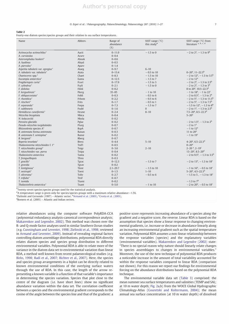
Of the 41 species and species groups identified, 27 were selectedfor statistical analysis (Table 2; Appendix C). The 14 excluded species,each with a cumulative relative abundance of less than 1% in all 52samples and/or a scattered distribution pattern, were not consideredfor these reasons.

Relative abundance plots of 26 selected species and species groupsin relation to the mean summer sea surface temperature are providedin Fig. 4. Eighteen prominent species and species groups were plottedon the basis of their common distribution in the study area. Thebiogeographic analysis and subsequent statistical analysis of specieswith respect to environmental variables was initially undertaken onall samples recovered, whereas the analyses of accumulation rateswere undertaken on two latitudinal transects, one with 10 samplesaround 120°W from 55°S to 70°S (referred to below as the westerntransect) and the second with 21 samples around 90°W from 50°S to70°S (the eastern transect).

3.3. Data processing

The raw counts were transformed to relative abundances in orderto map the diatom distributions. A further logarithm-based transfor-mation was performed as a prerequisite of the canonical redundancyanalysis using the following equation:

Y = LOG10ðrelative abundance × 10 + 1Þ ð1Þ

The determination of species accumulation rates (AR) wascalculated using two equations. First, the diatom valve concentrationper gram dry sediment was calculated:

Diatom valves= g = ð1=wtÞ × ðcsp= tpÞ × ðsusp= splitÞ× ðdiatom valve number = traverseÞ;

ð2Þ

where wt is the dried sample weight in grams, csp is the cover sliparea (254.5 mm2), tp is the area of the counted traverse (4.5 mm2),susp is the initial volume of processed diatom suspension (55 ml),split is the volume of suspension pipetted onto the cover slip (from6.5×10−3 to 4.9×10−1 ml) and traverse is the number of traversesfully counted under the light microscope (from 1 to 10).

The results of Eq. (2) were then multiplied with the bulksedimentary accumulation rate (AR) previously determined fromthorium isotopes (Geibert et al., 2005):

Diatom valve AR ½diatom valves m−2yr−1� = diatom valves= g

× bulk AR½g m−2yr−1�;ð3Þ

resulting in total diatom valve AR and values for specific species andspecies groups for the 31 samples (Table 1) along the two transects.For the 18 more prominent species and species groups the AR werecompared to the oceanic frontal system and the maximum averagesummer and winter sea ice concentrations along both transects.

3.4. Statistical methodology

To determine which environmental gradients in the upper watercolumn might influence the spatial distribution of the diatoms in thesediments, the statistical method of polynomial canonical redundancyanalysis (RDA) was applied to the diatom´s logarithm-transformed



relative abundances using the computer software PolyRDA-CCA(polynomial redundancy analysis-canonical correspondence analysis;Makarenkov and Legendre, 2002). This method was chosen over theR- and Q-mode factor analyses used in similar Southern Ocean studies(e.g. Cunningham and Leventer, 1998; Zielinski et al., 1998; reviewedin Armand and Leventer, 2009). Instead of revealing regional factorscontrolling diatom assemblage distributions, polynomial RDA directlyrelates diatom species and species group distribution to differentenvironmental variables. Polynomial RDA is able to relate more of thevariance in the diatom data set to environmental variation than linearRDA, a method well known from recent palaeoecological studies (e.g.Birks, 1998; Radi et al., 2007; Richter et al., 2007). Here, the speciesand species group arrangements in a biplot can be directly related toknown environmental conditions of the overlying surface watersthrough the use of RDA. In this case, the length of the arrow re-presenting a known variable is a function of that variable's importancein determining the species variation. Species that plot close to thecentre of the diagram (i.e. have short lines) show no significantabundance variation within the data set. The correlation coefficientbetween a species and the environmental gradient corresponds to thecosine of the angle between the species line and that of the gradient: a

positive score represents increasing abundance of a species along thegradient and a negative score, the reverse. Linear RDA is based on theassumption that species show a linear response to changing environ-mental gradients, i.e. increase or decrease in abundance linearly alongan increasing environmental gradient such as the spatial temperaturevariation. Polynomial RDA assumes a non-linear relationship betweenthe response variables (species) and the explanatory variables(environmental variables). Makarenkov and Legendre (2002) state:“There is no special reason why nature should linearly relate changesin species assemblages to changes in environmental variables.”Moreover, the use of the new technique of polynomial RDA producesa noticeable increase in the amount of total variability accounted forwithin the response variables compared to linear RDA (comparisonnot shown). For this reason we report our findings for environmentalforcing on the abundance distributions based on the polynomial RDAtechnique.

The environmental variable data set (Table 3) comprised: themean summer sea surface temperatures and salinities (TEMP and SAL;at 10 m water depth; Fig. 2a,b) from the WOCE Global HydrographicClimatology-Atlas (Gouretski and Koltermann, 2004); the meanannual sea surface concentration (at 10 m water depth) of dissolved

Table 2Fourty-one diatom species/species groups and their relation to sea surface temperatures.

Name Abbrev. Range ofabundance(%)

SSST range (°C)this study#

SSST range (°C) fromliterature a, b, c, d

Actinocyclus actinochilus* Aacti 0–11.0 −1.5 to 0 −2 to 2a, −1.3 to 9b

A. curvatulus Acurv 0–0.4Asteromphalus hookeri* Ahook 0–0.6A. hyalinus Ahyal 0–0.5A. parvulus* Aparv 0–1.4Azpeitia tabularis var. egregius* Ataeg 0–9.7 6–10A. tabularis var. tabularis* Atata 0–13.4 −0.5 to 10 0–20a, 11–22.3b

Chaetoceros spp.* Chaet 0–8.3 −1.5 to 10 −2 to 12a, −1.3 to 3.5b

Eucampia antarctica* Eanta 0–12.5 −1.5 to 7 −2 to 12a

Fragilariopsis curta* Fcurt 0–17.9 −1.5 to 3 −2 to 2a, −1.3 to 2.5b

F. cylindrus* Fcyli 0–2.1 −1.5 to 0 −2 to 2a, −1.3 to 3b

F. doliolus Fdoli 0–0.2 8 to 20a, 10.5–22.3d

F. kerguelensis* Fkerg 35–85 −1 to 10 −1 to 18a, −1 to 22c

F. obliquecostata* Fobli 0–0.3 −0.5 to 6 −2 to 0.5a, −1.3 to 2b

F. rhombica* Frhom 0–2.2 −0.5 to 6 −2 to 5a, −1.3 to 11.5b

F. ritscheri* Frits 0–1.7 −0.5 to 1 −2 to 5a, −1.3 to 7.5b

F. separanda* Fsepa 0–7.3 −1.5 to 7 −1.5 to 12a, −1.3 to 8b

F. sublinearis Fsubl 0–1.6 0 −2 to 1a, −1.3 to 2.5b

Hemidiscus cuneiformis* Hcune 0–2.4 8–10 7.5–20a, 8.5–22.3d

Nitzschia bicapitata Nbica 0–0.4 5–20a

N. kolaczeckii Nkola 0–0.2Porosira glacialis Pglac 0–0.2 −2 to 1.5a, −1.3 to 2b

Pseudo-nitzschia turgiduloides Pturg 0–0.7 −2 to 1a

Rhizosolenia species A* RspA 0–0.7 −1 to 12a

R. antennata forma antennata Ranan 0–0.3 11 to 20a

R. antennata f. semispina* Ranse 0–0.2 −1 to 19c

R. bergonii* Rberg 0–0.7Roperia tesselata* Rtess 0–4.4 5–10 4–20a, 6.5–22.3d

Thalassionema nitzschioides f. 1* Tnif1 0–0.5 0–20a

T. nitzschioides group* Tnigr 0–3.6 2–10 2–20 a, 2–19c

T. nitzschioides var. parva Tnipa 0–0.4 13–20a, 8.5–20d

Thalassiosira antarctica Tanta 0–0.2 −2 to 9.5a, −1.3 to 3.5b

T. frenguelliopsis Tfren 0–0.3T. gracilis* Tgrac 0–12.3 −1.5 to 7 −2 to 13a, −1.3 to 18c

T. gravida Tgrav 0–0.2T. lentiginosa* Tlent 2.1–29.7 −1.5 to 10 −1 to 16a, −0.5 to 18c

T. oestrupii* Toest 0–1.5 1–10 5–20a, 4.5–22.3d

T. oliverana* Toliv 0–2.7 −0.5 to 6 −1.5 to 5 , −1.3 to 18c

T. trifulta* Ttrif 0–0.7T. tumida Ttumi 0–0.2 −1.3 to 7b

Thalassiothrix antarctica* Txant 0–5.0 −1 to 10 −2 to 20a, −0.5 to 18c

⁎Twenty-seven species/species groups used for the statistical analysis.#A temperature range is given only for species/species groups with a maximum relative abundance N1.5%.aZielinski and Gersonde (1997) – Atlantic sector; bArmand et al. (2005), cCrosta et al. (2005),dRomero et al. (2005) – Atlantic and Indian sectors.



nitrate (NO3; Fig. 2c), phosphate (PO4; Fig. 2d) and silicon (Si; Fig. 2e)obtained from the World Ocean Atlas 2005 (Garcia et al., 2006); andtwo variables reflecting the surface water structure, the mean mixedlayer depth in summer (MLD; Fig. 2f) and the mean annual waterdensity between 0 m and 75 m depth gained from the LEVITUS94World Ocean Atlas (Monterey and Levitus, 1997). The variable N (inrad s−1) represents the mean annual Brunt–Väisälä-frequency foreach station, calculated from water densities as a measure of thestratification of the upper water column between 0 m and 75 mwaterdepth (after Vink, 2004):

N = √ð9:8 × δDÞ= ð1026 × δzÞ;

where δD represents the density difference over the distance δz (inthis case 75 m, at which the depth interval covers the range ofsummer MLD variation). Higher values of N represent increasedstratification (Fig. 2g). Finally the mean winter (WSIC; Fig. 2h) andsummer (SSIC; Fig. 2i) sea ice concentrations (Schweitzer, 1995) wereused to determine the influence of sea ice on the species distribution.

4. Results

4.1. Diatom occurrence and species distribution pattern

Highest diatom concentrations in surface sediments (up to185×106 valves/g dry sediment) and best preservation occured inthe western and central part of the study area, approximatelybetween the SAF and the southern ACC-boundary (Fig. 3, Table 1).In contrast, the samples from the continental slope of the AmundsenSea were characterised by mid-ranging diatom concentrations (10–40×106 valves/g dry sediment) and moderate preservation. Thecontinental slope is affected by channeling and multiple debris flowsand turbidites (Fig. 3). The lowest diatom concentrations (0.5–3×106

valves/g dry sediment) and moderate to poor diatom preservationoccurred at four sample sites, all located in the southwestern sector ofthe study area, which is affected by year-round sea ice cover (Fig. 2i).North of the SAF, diatom concentrations were also low to mid-ranging(20–40×106 valves/g dry sediment; Fig. 3). Here, diatom preservationwas generally observed as moderate. The distribution pattern ofdiatom valve concentration was mirrored by the diatom valve ARs,

Fig. 4. Relative abundances of the 26 diatom species and species groups used in the statistical analysis. Open circles represent samples from the western sector of the study area,closed circles represent samples from the eastern sector (sectors are divided by the 100°W meridian). For diatom name abbreviations see Table 2.



calculated on the basis of 230Th-normalised flux rates from Geibertet al. (2005). The diatom valve ARs obtained from the westerntransect were generally one order of magnitude higher than thosefrom the eastern transect (Fig. 5a,b). Highest values (8–10×108

valves m−2 yr−1) were encountered around 120°W between the SAFand the northern SSIZ, extending over ca. 900 km between 60°S and68°S (Fig. 5a). This pattern is mirrored by the BSi content of thesediment and the BSi ARs, reachingmaximumvalues between 70–80%and around 60 mmol m−2 yr−1, respectively (Fig. 5c,e). The latitudi-nal pattern of diatom valve ARs obtained from the eastern transect isless clear and this also accounts for the BSi content and itsaccumulation rates (Fig. 5b,d,f). Highest diatom valve ARs (around

20×107 valves m−2 yr−1) have been encountered between 62°S and68°S, which is south of the APF and north of the maximum meansummer sea ice extent (SSI), respectively. This is similar to the patternof the BSi accumulation (around 12 mmol m−2 yr−1), while the BSivalues only reach around 15% of the total sediment content. A distinctpeak in all three parameters occurs north of the SAF, with diatom ARaround 12×107 valves m−2 yr−1, BSi content around 30% and BSi ARsaround 10 mmol m−2 yr−1.

In the following paragraph, the biogeographic distribution of 18selected diatom species and species groups and the accumulation rate(AR) pattern along the western and eastern transects are described inalphabetical order. The observed summer sea surface temperature

Table 3Environmental variables used in the statistical analysis.

Station Temperature a

(°C)Salinity a

(p.s.u)Nitrateconcentration(μmol L−1)b

Phosphateconcentration(μmol L−1)b

Siliconconcentration(μmol L−1)b

Mixedlayer depth(m) c

Brunt–Väisälä-frequency(×10−6 rad s−1) c

Summer sea iceconcentration(%)d

Winter sea iceconcentration(%)d

PS2546-1 −1.28 33.58 23.95 1.46 61.86 14.68 256.74 54 87PS2547-2 −1.37 33.56 23.87 1.58 60.37 12.89 279.29 31 84PS2548-2 −0.93 33.55 23.93 1.62 59.25 12.83 295.43 31 84PS2550-2 −0.75 33.53 24.21 1.68 55.44 12.87 308.61 31 84PS2657-1 9.45 34.05 13.68 1.26 3.86 47.95 203.32 0 0PS2659-2 9.33 34.07 16.33 1.23 4.86 58.31 222.01 0 0PS2661-4 8.78 34.12 16.75 1.16 3.74 64.97 221.20 0 0PS2663-4 8.29 34.14 16.35 1.16 2.93 79.43 215.38 0 0PS2664-4 8.07 34.15 16.37 1.16 2.78 83.02 215.38 0 0PS2667-5 7.01 34.15 16.88 1.19 2.34 91.75 212.88 0 0PS2668-1 5.97 34.12 18.23 1.29 2.44 92.70 214.41 0 0PS2675-4 5.48 34.10 19.23 1.36 2.89 88.37 215.47 0 0PS2676-1 5.26 34.09 19.83 1.40 3.33 81.68 217.53 0 0PS2677-4 4.60 34.06 21.07 1.47 4.89 70.11 220.49 0 0PS2678-2 3.91 34.00 22.57 1.55 7.85 50.81 228.17 0 0PS2679-1 3.33 33.93 23.40 1.59 9.47 43.62 234.08 0 0PS2680-4 2.62 33.83 24.03 1.61 10.85 38.17 243.19 0 0PS2684-1 −0.48 33.40 25.00 1.69 35.95 7.03 345.05 0 79PS2686-2 −0.20 33.51 25.39 1.68 32.89 10.93 330.09 24 80PS2687-5 −0.16 33.47 24.71 1.64 26.71 10.98 334.25 3 81PS2688-4 0.09 33.50 24.46 1.61 21.52 13.50 316.86 0 49PS2690-1 0.81 33.60 24.41 1.59 14.73 23.22 272.49 0 17PS2691-1 0.84 33.60 24.41 1.60 14.49 23.49 274.07 0 17PS2692-1 0.94 33.62 24.43 1.60 14.20 25.86 272.49 0 17PS2694-1 1.15 33.64 24.55 1.61 12.81 29.74 257.28 0 14PS2695-1 0.96 33.61 24.46 1.60 13.73 25.03 275.20 0 14PS2696-4 0.93 33.70 24.39 1.59 12.25 43.08 238.76 0 1PS2697-1 2.19 33.83 24.00 1.57 10.35 57.91 238.76 0 1PS2699-5 4.70 34.05 22.01 1.48 6.25 74.10 224.76 0 0PS2700-5 4.88 34.07 21.07 1.44 4.96 78.72 220.71 0 0PS2701-2 5.09 34.09 19.92 1.38 3.72 83.55 217.80 0 0PS2703-2 5.83 34.12 18.39 1.30 2.49 92.33 214.41 0 0PS2714-6 6.00 34.13 17.85 1.26 2.37 91.02 214.25 0 0PS2715-3 6.28 34.13 17.32 1.24 2.33 89.44 214.89 0 0PS2716-2 7.04 34.14 16.39 1.23 2.77 83.76 217.44 0 0PS58/252-1 −0.27 33.38 24.02 1.58 22.59 8.51 338.19 0 76PS58/253-2 −0.62 33.43 25.53 1.67 43.36 4.42 364.73 1 81PS58/254-2 −0.63 33.44 25.56 1.68 44.54 4.95 362.10 1 81PS58/256-1 −0.44 33.41 24.74 1.60 31.70 4.54 355.48 0 81PS58/258-1 −0.43 33.40 24.42 1.57 28.32 4.83 353.37 0 81PS58/265-1 −0.07 33.58 24.51 1.72 38.74 19.89 285.69 0 67PS58/266-4 0.25 33.62 24.63 1.73 28.90 25.32 267.17 0 13PS58/268-1 1.08 33.74 24.60 1.72 15.89 35.16 238.18 0 0PS58/269-4 1.41 33.75 24.46 1.70 13.05 40.84 231.60 0 0PS58/270-1 1.92 33.82 24.08 1.63 11.64 43.54 234.03 0 0PS58/272-4 2.57 33.97 23.34 1.54 7.62 46.53 228.05 0 0PS58/274-4 3.94 34.05 22.27 1.46 5.14 52.46 227.43 0 0PS58/276-1 5.17 34.13 19.65 1.34 3.10 54.12 224.71 0 0PS58/280-1 5.64 34.11 19.06 1.35 2.81 87.64 215.47 0 0PS58/290-1 5.81 34.12 18.41 1.30 2.50 92.24 214.41 0 0PS58/291-3 6.02 34.13 18.31 1.29 2.49 92.36 214.89 0 0PS58/292-1 6.18 34.13 18.23 1.29 2.55 86.64 214.61 0 0

a Sea surface (10 m water depth) summer temperature and salinity taken from the WOCE Global Hydrographic. Climatology Atlas (Gouretski and Koltermann, 2004).b Mean annual sea surface (10 m water depth) concentration of dissolved nitrate, phosphate and silicon; variables derived from theWorld Ocean Atlas 2005 (Garcia et al., 2006).c Mixed layer depth in summer and the Brunt–Väisälä-frequency (N) calculated from the mean annual water density fromwater depth of 0 m and 75 m; data from the LEVITUS 94

World Ocean Atlas (Monterey and Levitus, 1997).d Winter (WSI) and summer (SSI) sea ice concentrations after Schweitzer (1995).



(SSST) ranges for each species and species group are summarised inTable 2.

Actinocyclus actinochilus displayed significant relative abundancesat the southernmost sites, an area on the western transect that isaffected by year-round sea ice (Figs. 2h,i and 6a). Average summer seasurface temperatures (SSST) in this area ranged between −1.5 and0 °C (Fig. 2a).

Azpeitia tabularis var. egregius was only encountered along theeastern transect. Higher abundances were restricted to an area northof the SAF, at SSST around 6 °C (Figs. 4 and 6d,e).

Azpeitia tabularis var. tabularis displayed a broader zone of occurrencethan its variety egregius. Amounts N5% of the total assemblages occurredbetween SSSTs of 10 °C in the SAZ and 2 °C (POOZ) in the study area andmaximum values were centred around 9 °C (Fig. 7a). Southernmostoccurrences were observed in the SSIZ (Fig. 7a). At the western transectthe A. tabularis var. tabularis AR mirrored the pattern of the total diatomvalveARas a result of the lackof a latitudinal abundancegradient (Fig. 7b).Such a gradient occurred in the eastern transect and led to the highestspecies AR values in its northern section (Fig. 7c).

Relative abundances of the Chaetoceros spp. group revealed abimodal distribution pattern with occurrences N5% south of the SSI(SSST around −1 °C) and north of the SAF at SSST around 6 °C(Figs. 2a,i, and 7d).

The Eucampia antarctica group has been encountered over a largeenvironmental range. Highest relative abundances (N5%) occurred inthe area affected by winter and summer sea ice, but also at sites northof the SAF (SSST 6–7 °C) where around 3% of the preserved diatomassemblages consisted of the E. antarctica group (Figs. 2 and 8a).

The archetypal sea ice indicator species, Fragilariopsis curta(Gersonde and Zielinski, 2000; Armand et al., 2005) displayedabundances N2% of the total diatom assemblage. The species wasrestricted to the southernmost study area, where sea ice cover is nearannually persistent (Figs. 2 and 8d). Low abundances (b1%) have beenobserved as far north as the area of the SAF (Fig. 8d). Consequently theARs calculated for F. curta show a clear S–N gradient in both transects(Fig. 8e,f).

Fragilariopsis kerguelensis represents the most dominant species inthe study area. Except for the southernmost sample site (PS2546-1)and four sites located in the southernmost SAZ (eastern transect), F.kerguelensis contributes N50% to the assemblages (Fig. 9a). Conse-quently the pattern of the F. kerguelensis ARs clearly reflects the totaldiatom valve and the BSi ARs (Figs. 5 and 9b,c). At the westerntransect F. kerguelensis ARs reached highest values ranging between 5and 8×108 valves m−2 yr−1 in the zone of highest BSi deposition.This makes F. kerguelensis valves the major contributor to the BSipreserved at the sea floor.

Fragilariopsis rhombica and Fragilariopsis ritscheri occurred poorlyacross the two transects. Highest abundances and species ARs werenoted in samples from the eastern transect specifically in between themean SSI and WSI boundaries (Figs. 9d,f and 10a,c).

The relative abundance distribution of Fragilariopsis separandaclearly shows a N–S increase from the SAZ to the SSIZ. Overall higherrelative abundances occurred in the western sector of the POOZ.Lowest relative abundances occurred at the southernmost samplesites (western transect), located in an area affected by winter andsummer sea ice, and at the northernmost sites (eastern transect),

Fig. 5. Total diatom accumulation rates (diatom valve AR; plots a,b), biogenic opal relative abundance (BSi; from Geibert et al., 2005; plots c, d) and biogenic opal accumulation rates(BSi AR; from Geibert et al., 2005; plots e, f) compared between the 120°W and the 90°W transects. Abbreviations: APF: Antarctic Polar Front; sACCF: southern ACC Front; SAF:Subantarctic Front; SSI: maximum average summer sea ice extent; WSI: maximum average winter sea ice extent.



where SSSTN8 °C. Maximum abundances and valve ARs occurred inthe POOZ and the SSIZ where SSSTs range between 0 and 4 °C (Figs. 2aand 10d,e,f).

The typical warm water species Hemidiscus cuneiformis (Zielinskiand Gersonde, 1997; Romero et al., 2005) was present exclusively atnorthernmost sample sites (eastern transect), where SSSTs were N8°(Figs. 4 and 11a,b).

Roperia tesselata, another warm water species (Zielinski andGersonde, 1997; Romero et al., 2005), showed a larger range ofdistribution, extending as far south as the SAF (Fig. 11c,d,e). Highestabundances were referable to SSSTsN7 °C.

The Thalassionema nitzschioides group exhibited greatest abun-dances north of 64°S (SSST N3 °C) and the influence of the seasonalsea ice (Figs. 4 and 12a,b,c). Along the western transect, highest ARs

occurred north of the APF, whereas along the eastern transect acomparably lower AR maximum occurred south of the APF.

The Thalassiosira gracilis group displayed highest relative abun-dances in the southern section of the eastern transect, at SSSTs between−1 and 1 °C (Fig. 4). In the western transect, relative abundances werecomparably lower than in the east (Fig. 12d), but ARs along 120°Wwerehigher compared to the 90°W transect, with a broader distributionrange from the southern SAZ to the SSIZ. Maximum ARs occurred alongboth transects in the SSIZ between WSI and SSI. (Fig. 12e,f).

Thalassiosira lentiginosa showed highest relative abundance atthe eastern transect between the Antarctic Zone and the SAZ,which corresponds to a SSST range from 4 to 8 °C. The zone of highT. lentiginosa ARs expands further southward to about 65°S whereSSST are 2 °C (Figs. 2a and 13a,b,c). The rather large and strongly

Fig. 6. Relative abundance maps and valve accumulation rates (AR) of the diatom species Actinocyclus actinochilus (a, b, c) and Azpeitia tabularis var. egregius (d, e). Abbreviations:APF: Antarctic Polar Front; sACCF: southern ACC Front; SAF: Subantarctic Front; SSI: maximum average summer sea ice extent; WSI: maximum average winter sea ice extent.



silicified valves of T. lentiginosa represent another prominent contrib-utor to the total diatom AR (Fig. 5a,b), inclusive of BSi % content at thesea floor (Fig. 5c,d), and the BSi AR latitudinal trends (Fig. 5e,f).

Thalassiosira oestrupii war encountered only rarely (b1.5% relativeabundance; Table 2) Their dominance and highest AR values werefound north of the SAF, where SSSTs are N5 °C (Figs. 2a and 13d,e,f).

The heavily silicified Thalassiosira oliverana exhibited higherrelative abundances and valve ARs in the AZ along the easterntransect (SSSTs −0.5 to 4 °C; Figs. 2a and 14a,b,c). This speciesrevealed trace occurrence in the western transect (Fig. 14a).

The needle-shaped Thalassiothrix antarcticawas encountered at allsample sites, with exception to two southerly sites in the westerntransect affected by summer sea ice (Fig. 14d). The species abundanceswere greatest in the southern SAZ and POOZ across both transects,where SSSTs ranged between 3 and 8 °C (Figs. 4 and 14d).

The remaining 23 species and species groups preserved in thestudied set of samples showed no distinct distributional patterns dueto their low relative abundances, and resulted in negligible contribu-tions to the total diatom accumulation rates (not shown). Regardlessof the poor representation of certain species encountered, some ofthese species contribute to the variance in assemblage compositionwithin the polynomial RDA. These species are: Fragilariopsis cylindrus,Fragilariopsis ritscheri and Thalassiosira trifulta.

4.2. Polynomial canonical redundancy analysis (polynomial RDA)

The statistical analysis of 27 selected species and species groupsfrom the 52 samples (Table 2) via the polynomial RDA explains 69.6%total variance (r2=0.60; the given value is the cumulative percentageof the total pricipal component analysis (PCA) variance) in relation to

Fig. 7. Relative abundance maps and valve accumulation rates (AR) of the diatom species/species groups Azpeitia tabularis var. tabularis (a, b, c) and Chaetoceros spp. (d, e, f).Abbreviations as in Fig. 6.



the nine tested environmental variables, with 29.7% of varianceexplained by the first gradient and 15.6 % explained by the secondgradient (Table 4). The remaining 30.4% of variance was unexplainedby the nine tested variables andmay be due to a variety of unexploredfactors, but most likely the influence upon diatom preservation in thenorthern and southern zones of the study area compared to thecentral zone played an important role.

In the plot of sample distribution in relation to vectors reflectingthe different environmental variables tested (Fig. 15a), the vectors offirst order temperature (TEMP), salinity (SAL), and mixed layer depth(MLD) point in the direction of the lower left quadrant, whereas thevectors representing first order stratification (N) nitrate (NO3) andphosphate (PO4) point approximately in the opposite direction. Thecorrelation of the environmental variables exhibits a certain amount ofcovariance among these six variables (Table 5), potentially biasing the

results. The vectors reflect changing environmental conditions alongthe first canonical axis with decreasing temperature and salinity, andsimultaneous increase of the dissolved nutrients NO3, PO4 and silicon(Si) (and sea ice concentration).

Fig. 15b identifies the samples located far north of the SAF with thehighest negative values on the first canonical axis, and samplespositioned near the SSIZ with the highest positive values on the firstaxis. Changes in value of the first RDA-axis follow a latitudinal gradientwhere high negative values were associated with low latitude samplestations (b−0.5) in conjunctionwith the SAF in themost eastern sector,and largest positive values (N0.5) corresponding to samples at themaximum average winter sea ice extent (Fig. 2h). Thus, the gradient ofthefirst RDA-axis is assumed to reflect the relationship between speciesassemblages and one or more environmental variables (see Appendix Bfor the site scores of the polynomial RDA).

Fig. 8. Relative abundance maps and valve accumulation rates (AR) of the diatom species of the Eucampia antarctica group (a, b, c) and Fragilariopsis curta (d, e, f). Abbreviations as inFig. 6.



A simple linear regression (only shown for temperature) betweeneach variable and the first RDA-axis revealeds different coefficients ofdetermination (r2) for each variable (Table 6), with the strongestcorrelation observed with summer temperature (r2=0.941; Fig. 15c),followed by annual nitrate (r2=0.908), summer salinity (r2=0.819)and annual phosphate (r2=0.791) as secondary variance contribu-tors. The remaining variables were less strongly associated to the firstRDA-axis. For the second RDA-axis three variables could be signifi-cantly correlated (r2N0.2; after Pearson's test of correlation coefficientsignificance) with the variance along this axis (Table 6): annualdissolved silicon (0.418) and mean winter and summer sea iceconcentrations (0.264 and 0.646, respectively). This is in accordancewith the geographical distribution of the sample locations: highestpositive values on the second canonical axis are shown for the fourstations annually affected by sea ice (Fig. 15a).

The polynomial RDA diagram for the relationship between speciesand the environmental variables (Fig. 16) indicated positive correla-tion or negative correlation between single species (for abbreviationssee Table 2; see Appendix C for the species scores of the polynomialRDA) and vectors of environmental variables of first order (MLD, N,NO3, PO4, SAL, Si, SSIC, TEMP, and WSIC) and second order (MLD2, N2,NO3

2, PO42, SAL2, Si2, SSIC2, TEMP2, and WSIC2 ). Generally, the

environmental variable analysis shows strong covariance betweenTEMP, SAL, MLD, NO3, PO4 and N on one side and between Si, SSIC andWSIC on the other (Table 5). Focusing on the temperature/nutrientgradient, as the predominant factor in the site-related RDA (Fig. 15a),the species-related analysis reveals positive correlation only withT. oestrupii with first order TEMP, SAL and MLD, whereas F. curta andF. cylindrus show a negative correlation to these three variables. Incontrast, F. rhombica, F. ritscheri, F. separanda and T. gracilis are

Fig. 9. Relative abundance maps and valve accumulation rates (AR) of the diatom species Fragilariopsis kerguelensis (a, b, c) and Fragilariopsis rhombica (d, e, f). Abbreviations as inFig. 6.



negatively correlated to the second order TEMP2. Species with nocorrelation to any of the environmental variables, either due to theirvery low relative abundance (e.g. Fragilariopsis obliquecostata; Fig. 4)or their equally high distribution across the whole temperature range(e.g. F. kerguelensis; Fig. 4) show very short or no vector length(Fig. 16). The vectors of A. tabularis var. egregius, H. cuneiformis and R.tesselata imply a relationship of the species abundance to the first andsecond order sea surface summer temperature and NO3

2/PO42 (Fig. 16).

On the other hand, the variance in F. curta and A. actinochilus, and to alesser degree F. cylindrus and E. antarctica group, are correlated eitherwith changes in the mean annual dissolved silicon concentration ofthe upper water column or to the variance in winter and summer seaice concentrations. However, the relationship between the diatomassemblage compositions and sea ice/dissolved silicon variation(second RDA-axis) is less distinct than the relationship with the

temperature/nutrient variation (first RDA-axis) in explaining themain variance observed in the data set (Table 4).

5. Discussion

5.1. Diatom accumulation rates and opal deposition

The diatom valve concentration and 230Th-normalised valve ARs,as well as BSi concentration (weight percent) and 230Th-normalisedBSi ARs display distinct differences between the eastern (90°W) andwestern (120°W) transects in terms of their magnitude and theirlatitudinal distribution pattern (Fig. 5). The magnitude of BSideposition and the maximum deposition of BSi in a region betweenthe SAF and the northern SSIZ observed along thewestern transect aresimilar to the values and the distribution pattern of BSi described by

Fig. 10. Relative abundance maps and valve accumulation rates (AR) of the diatom species Fragilariopsis ritscheri (a, b, c) and Fragilariopsis separanda (d, e, f). Abbreviations as inFig. 6.



Geibert et al. (2005) from the Atlantic sector of the Southern Ocean.Similarly, our results match 230Th-normalised BSI observationsdetermined from the western Pacific sector around 170°W (Sayleset al., 2001) and the Indian sector along 110°E (François et al., 1997),where a zone of high BSi deposition spans between 800 and 1000 kmin latitude. However, BSi ARs from the western Pacific, the Indian andAtlantic sectors may exceed the values at our 120°W transect byfactors of 2 to 5 (DeMaster, 2002). Because diatom valve accumulationrates in this paper are the first to be presented from the SouthernOcean, comparisons concerning the contribution of diatom species tothe deposited BSi in other sectors of the Southern Ocean can only bebased on estimates of averaged BSi AR values and diatom speciesabundances from the same area. Diatom species distributions insurface sediments presented from the Atlantic and the Indian sectors(Zielinski and Gersonde, 1997; Crosta et al., 2005) indicate that F.kerguelensis represents the dominant species of the Southern Ocean

open-ocean opal deposition, as documented by this study of the120°W transect. Distinctly lower diatom valve and BSi depositionencountered along the 90°W transect (Fig. 5b,f) mark a sector ofreduced biogenic opal deposition in the eastern South Pacific, whichextends into the area of the Drake Passage (Geibert et al. 2005). Suchreduction in BSi accumulation has already been remarked byDeMaster (1981). A distinct reduction of the Southern Ocean opalbelt between 120°W and the Drake Passage has also been predicted byan annually averaged version of the Hamburg Ocean Carbon Cyclemodel (Ragueneau et al., 2000). The presence of this Southern Ocean“diatom deposition gap” requires explanation. Generally, macronu-trient concentrations decline from west to east in the study area(Fig. 2), which may be related to the channelling effect of the DrakePassage. However, according to Holm-Hansen et al. (2005) thispattern should not have a distinct effect on biological productivity.They report overall low productivity between 140°W and 70°W (see

Fig. 11. Relative abundance maps and valve accumulation rates (AR) of the diatom species Hemidiscus cuneiformis (a, b) and Roperia tesselata (c, d, e). Abbreviations as in Fig. 6.



also Moore and Abbott, 2000), as a result of continental source traceelement availability in this area. As such, it is unlikely that differencesin diatom production are responsible for the uneven deposition ofdiatoms in the eastern and western sector of the study area and itfollows that other factors must be considered to explain the observeddecoupling of primary production from the distribution of diatomvalve abundances and BSi preservation.

The discovery that bulk vertical sediment fluxes at both transectsare of similar magnitude (Table 1), which results from higherterrigenous flux rates along the eastern transect (Geibert et al.,2005), helps to explain the inter-basin difference. Such a pattern is notsupportive of an east-west differentiation of BSi deposition ratesarising from generally lower sedimentation rates at 90°W, as a resultof increased bottom water winnowing in the vicinity of the Drake

Passage. However, increased deposition of terrigenous components inthe deep basin of the Bellingshausen Sea may have an effect on thepreservation of biogenic opal after its deposition at the sea floor.Increasing sediment ratios of terrigenous to BSi content has beenreported as leading to a decrease in silicic acid concentration in porewaters and a reduction of BSi preservation (Ragueneau et al., 2000).Indeed, the sedimentary environments in the areas of the eastern andwestern transects are distinct. While the 90°W transect located acrossthe flat Bellingshausen abyssal plain is supplied by distal turbiditesfrom the tectonically active Antarctic Peninsula region (Nitsche et al.,2000; Robertson Maurice et al., 2003), along the 120°W transectdeposition of terrigenous components by turbidites from the Antarcticmargin is restricted by an undulated bottom topography, especiallynorth of site PS58/265 (Fig. 1). Thus, we conclude the biogenic flux

Fig. 12. Relative abundance maps and valve accumulation rates (AR) of the diatoms species groups Thalassionema nitzschioides group (a, b, c) and Thalassiosira gracilis (d, e, f).Abbreviations: APF: Antarctic Polar Front; sACCF: southern ACC Front; SAF: Subantarctic Front; SSI: maximum average summer sea ice extent; WSI: maximum average winter sea iceextent.



into the sediments is prone to higher dilution by terrigenous materialalong the eastern transect than in the western sector, accounting forthe differantiation in diatom AR and BSi AR values presented here.

5.2. Diatom species distribution

The observed diatom distribution patterns are closely related tothe oceanographic zones and themean sea ice seasonal maxima in thestudy area and coincides well with the diatom distribution reportedfrom other sectors of the Southern Ocean (Zielinski and Gersonde,1997; Armand et al. 2005; Crosta et al., 2005; Romero et al., 2005).This pattern is not significantly disturbed, either by the east–westgradient in diatom accumulation and preservation or by the presenceof large sediment drifts, debris flows and off-shore reaching channelsystems at the Antarctic continental margin (Fig. 3). At the siteslocated near the continent, neither down-slope transport of neritic

diatoms from the Antarctic shelf environment nor reworking of olderfossil species could be detected.

5.2.1. Subantarctic Zone (SAZ)Overlooking the elevated high abundances of species with large

temperature ranges (e.g. F. kerguelensis, T. lentiginosa), the SAZ diatomassemblage was found to be characterised by typical warmer waterdwellers, such as A. tabularis (both varieties), H. cuneiformis, R.tesselata, the T. nitzschioides group and T. oestrupii. This observation isin accordance with previous work carried out in the same area.Kozlova (1966) reported F. kerguelensis and T. lentiginosa to bedominant species in Subantarctic sediments of the Pacific sector.Considering that BSi and diatom valve preservation both decreased inthe SAZ (Figs. 3 and 5), it can be assumed that the relative abundancesof the heavily silicified F. kerguelensis and T. lentiginosa in this zone

Fig. 13. Relative abundance maps and valve accumulation rates (AR) of the diatom species Thalassiosira lentiginosa (a, b, c) and Thalassiosira oestrupii (d, e, f). Abbreviations as inFig. 6.



were enhanced as a result of their higher preservation efficiency(Burckle and Cirilli, 1987; Pichon et al., 1992a,b).

Remarkably, the variety Azpeitia tabularis var. egregius occurred inhigher numbers only along the eastern transect north of the SAF

(Fig. 6). This distribution pattern of A. tabularis var. egregius suggests alower tolerance to colder temperatures compared to the variety ta-bularis (Fig. 4). This assumption is supported by the results of thepolynomial RDA, showing the vector of A. tabularis var. egregius topoint more in the direction of the environmental variable vectorsTEMP and TEMP2 then the vector of A. tabularis var. tabularis (Fig. 16).However, such a difference in the distribution pattern of both varietieshas not been observed in other sectors of the Southern Ocean (e.g.Zielinski and Gersonde, 1997; Romero et al., 2005).

A census of diatom assemblages preserved in surface sedimentsfrom the Atlantic and Indian sectors of the Southern Ocean generallyconfirms our biogeographic distribution results obtained from thesoutheastern Pacific sector. Roperia tesselata and H. cuneiformis wereexclusively encountered north of the SAF in the Atlantic and Indiansectors (Romero et al., 2005), with the exception of rare findings ofR. tesselata in the Atlantic sector SAZ (Zielinski and Gersonde, 1997).

Fig. 14. Relative abundance maps and valve accumulation rates (AR) of the diatom species Thalassiosira oliverana (a, b, c) and Thalassiothrix antarctica (d, e, f). Abbreviations as inFig. 6.

Table 4Polynomial canonical redundancy analysis (RDA) results.

Polynomial RDA of 52 samples, 27 species/taxa, 9 environmental variables

Axes 1 2 3 4

Canonical Eigenvalues 1.39 0.73 0.43 0.18% of the total PCA variance 29.72 15.59 9.12 3.90Cumulative % of the total PCA variance 29.72 45.31 54.43 58.33Cumulative % of the canonical variance 42.69 65.08 78.18 83.78

PCA: Principal Component Analysis (the PCA is the first element of the polynomialRDA).



Other typical warm water dwellers, such as Alveus, Fragilariopsisdoliolus, Thalassionema nitzschioides var. parva and Rhizosoleniabergonii, which have been encountered in the Atlantic and Indiansectors only north of the Subtropical Front or with a southernmostoccurrence boundary in the northern SAF (Zielinski and Gersonde,1997; Romero et al., 2005) have been found scattered and at very lownumbers (b1% of assemblage), with exception to A. marinus, whichwas not detected in the set of samples studied (Table 2).

Significantly, a zone of increased occurrences of Chaetoceros spp.group and the E. antarctica group was observed along the 90°Wtransect in the southernmost SAZ close to the SAF. Althoughwedid notdistinguish between the two E. antarctica varieties reported by Fryxelland Prasad (1990), E. antarctica frustules observed in the SAZ mightbelong to E. antactica var. recta, whereas the increased occurrenceof the E. antarctica group in the SSIZ (Fig. 8a) may be related toE. antarctica var. antarctica. Plankton studies confirm increased Chae-toceros and E. antarctica occurrences around 60°S in the study area

(Hasle 1969; Fenner et al., 1976), but such distribution patterns havenot been reported from previous surface sediment studies in theAtlantic and Indian sectors (Zielinski and Gersonde, 1997; Armandet al., 2005). de Baar et al. (2005) and Blain et al. (2007) have shownthat both, Chaetoceros spp. and Eucampia spp., were preferentiallyproduced at nutrient conditions with elevated Fe-content. DissolvedFe concentrations are generally very low in the eastern SouthernOcean Pacific because of its remoteness from upwind and upstreamcontinental Fe source areas (e.g. Mahowald et al., 2005), but indeed aFe-survey accomplished in the study area in late austral summer 1995has found a slight Fe-enhancement in surface waters around 60°S inthe PFZ (de Baar et al., 1999). Hints on the nature of the Chaetocerosresting spores can be derived from phytoplankton studies at 90°Wreported by Hasle (1969). Her analysis of the Brategg samples resultsin a maximum (up to 0.4 106 cells l−1) of Chaetoceros neglectus(belonging to the resting spore forming subgenus Hyalochaetae)around 60°S. Thus, the elevated numbers of Chaetoceros spp. spores

Fig. 15. a). Results of the polynomial Redundancy Analysis (RDA) showing variance in the diatom distribution (based on 26 selected species/species groups) in relation to theenvironmental variables of sea surface summer temperature (TEMP, TEMP2) and salinity (SAL, SAL2), mean annual surface water concentrations of dissolved nitrate (NO3, NO3

2),phosphate (PO4, PO4

2) and silicon (Si, Si2), mean annual stratification of the water column (expressed in the Brunt–Väisälä frequency; N, N2), the mean summer mixed layer depth(MLD, MLD2) and mean winter and summer sea ice concentrations (WSIC, WSIC2, SSIC, SSIC2). b. Spatial distribution of the site score values of the polynomial RDA (crosses: b−1.5;triangles:−1.5 to− 0.5; circles:−0.5 to 0.5; boxes: N 0.5). c. Regression plot of first axis polynomial RDA site scores versus sea surface summer temperature (SSST). The polynomialRDA accounts for 69.6% of total cummulative variance due to polynomial regression (mean coefficient of multiple determination=0.60) and implies SSST to be the predominantenvironmental variable correlated with the diatom distribution (r2=0.941).



found in the SAZ of the studied region might reflect the increasedproduction of C. neglectus in this area.

5.2.2. Polar Front Zone (PFZ) and Permanent Open Ocean Zone (POOZ)As observed in the southern SAZ, F. kerguelensis represented one of

the most prominent species of the PFZ and the POOZ of the southwestand central Pacific sector. The same finding was reported from theIndian and Atlantic sectors (Zielinski and Gersonde, 1997; Crosta et al.,2005). In spite of the eastward decrease in diatom preservation, thehighest F. kerguelensis abundances were encountered the length of the120°W transect. Along the 90°W transect the F. kerguelensis abun-dances were reduced by the occurrence of species such as A. tabularis,T. gracilis var. gracilis and T. oliverana (Figs. 6d, 7a,12d,14a). Thalas-siosira lentiginosa represented the second most abundant species,especially in the SAZ and northern POOZ. Prominent occurrences of

this species (N15%) are related to a narrower and higher temperaturerange (4.5–6.5 °C) than F. kerguelensis (Figs. 9a and 13a). This patternhas not been reported from the Atlantic and Indian sectors,where bothspecies have been related to a similar SSST range (Zielinski andGersonde, 1997; Crosta et al., 2005). Other species encountered tooccur widespreadly in the PFZ and the POOZ at significant abundances(N3%) and include A. tabularis, F. separanda, the T. nitzschioides group,T. gracilis, T. oliverana and Thalassiothrix antarctica.

Increased abundances of F. separanda (N3%) are associated with aSSST range between −0.5 and 4 °C and maximum abundances (N6%)occur between 0 and 1.5 °C, which is similar to the distribution rangereported by Zielinski and Gersonde (1997) from the Atlantic sector. Assuch, the F. separanda distribution extends into the SSIZ, a patternconsistent with the compilation of F. separanda distribution datapresented by Armand et al. (2005) from the Indian andAtlantic sectors(abundance N3% between −1 and 4 °C). Despite our study´s ratherlarge distribution range extending from the SSIZ into the SAZ (Fig. 10d)and summaries of F. separanda having never been reported from anystudies of sea ice samples (Zielinski andGersonde, 1997; Armand et al.,2005), Armand et al. (2005) labelled F. separanda as one of the majorsea ice related species, but also stated, that it had a “superficially poorrelationship to sea ice parameters”. They suggest that the widetemperature range results from lateral transport, but fail to explainwhy such transport mechanisms would only affect the distribution ofF. separanda and not that of other sea ice related species. Also, thebottomwater pathways in the SE Pacific sector, derived from pressurefield differences (Fig. 3; Reid, 1986), and the flow pattern of freshlyproduced bottom water, identified by chlorofluorocarbon concentra-tions (Orsi et al., 1999; Rodehacke et al., 2007), show for the area southof 60°S a coastal-parallel bottom water flow in a westerly directionrather than a northward bottom layer transport. Thus, at least for theeast Pacific sector, this makes lateral transport unlikely as anexplanation for the higher abundances of F. separanda in sedimentsof the northern POOZ and north of the APF. Plankton studies in thePacific sector (Hargraves, 1968) reported a broad distribution range of

Fig. 15 (continued).

Table 5Correlation matrix of the 9 environmental variables.

The grey bars highlight environmental variables covarying with others. The numbersindicate either strong positive or negative covariance if a threshold value of 0.8/−0.8 isexceeded.

Table 6Correlation between the first and second RDA-axes and the 9 tested environmentalvariables.

Environmental variables First RDA-axisa Second RDA-axisa

TEMP 0.941 0.017SAL 0.819 0.023NO3 0.908 0.010PO4 0.791 0.016Si 0.505 0.418MLD 0.748 0.026N 0.611 0.028SSIC 0.118 0.646WSIC 0.491 0.264

a The values represent the coefficient of determination (r2) for simple linarregressions between RDA-scores and environmental variables.



F. separanda in waters with temperatures between 1.2 and 8.7 °C,which makes it unlikely that F. separanda is a typical sea ice relatedtaxon. The distribution of this species suggests a preference for surfacewaters free of sea ice at least during the summer season.

The abundance of the T. nitzschioides group decreased towards thesouth and dropped to values below 1% of the total diatom assemblageat SSSTsb3 °C. A similar pattern that has been reported from theAtlantic and Indian sectors (Zielinski and Gersonde, 1997; Crosta et al.,2005). In contrast, Thalassiosira gracilis abundances increased towardsthe SSIZ and reached maximum abundances in the SSIZ. This patternrelates T. gracilisN4% to SSSTs ranging between−1 and 3.5 °C, which issimilar to the temperature relationship presented from the Atlanticand Indian sectors (Zielinski and Gersonde, 1997; Crosta et al., 2005),although Zielinski and Gersonde (1997) report occurrences N4%extending into waters with 6 °C during summer. Thalassiothrixantarctica displayed highest relative occurrences (5%) in the southeastPacific POOZ, but has been encountered at valuesN1% in a broader zoneextending from the SAF into the sea ice covered zone. Such a broadoccurrence range was also gathered from the Atlantic and Indian

sectors, reaching maximum values at a SSST range attributable to thenorthernPOOZ and the PFZ (Zielinski andGersonde, 1997; Crosta et al.,2005).

The general composition of the diatom assemblage observed in thePOOZ and SSIZ characterises these two zones as areas of lowerproductivity and lower organic carbon export, compared to other sectorsof the Southern Ocean. The overall dominance of F. kerguelensis valves onthe sea floor is a significant indicator in this respect. Studies on therelationship between phytoplankton productivity and trace metal supplyassumed that the lack of iron prevents the complete utilisation of ambientnitrate and influences phytoplankton species composition in open-oceanhigh nutrient low chlorophyll regimes (e.g. Hutchins and Bruland, 1998).Iron limitation increases the uptake of dissolved silicon, relative to nitrateand phosphorus. This led to the assumption that high grazing pressure onthe regeneratingmicrobial communities characteristic of the iron-limitedSouthern Ocean results in the accumulation of large, heavily silicifieddiatoms, such as F. kerguelensis, that drive the silicon pump (Smetaceket al., 2004). Consequently, higher biogenic opal accumulation in sedi-mentary records may reflect less productive surface water conditions

Fig. 16. Results of the polynomial RDA focused on the relationship between 26 diatom species/species groups (abbreviations are listed in Table 2) and the first and second order ofenvironmental variables of mean summer sea surface temperature (TEMP, TEMP2) and salinity (SAL, SAL2), mean annual surface water concentrations of dissolved nitrate (NO3,NO3

2), phosphate (PO4, PO42) and silicon (Si, Si2), mean annual stratification of the water column expressed in the Brunt–Väisälä frequency (N, N2), the mean summer mixed layer

depth (MLD, MLD2) andmeanwinter and summer sea ice concentrations (WSIC,WSIC2, SSIC, SSIC2). The RDA plot shows a strong positive relationship between species and variablespointing in the same direction, and a strong negative relationship for species and variables pointing in the opposite direction, with the significance of the relationship given by thearrow length. No correlation between the variables and species are given for perpendicular plots of species (shown as inset box).



instead of high export production. The assumption of lower carbon exportin the eastern Pacific sector compared to other Southern Ocean sectors issupported by the productivity studies of Arrigo et al. (1997, 1998) andmaypartially be a result of lower iron supply to thephotic zone (deBaar etal., 1999).

5.2.3. Seasonal Sea Ice Zone (SSIZ) and Sea Ice Zone (SIZ)The diatom assemblages in surface sediments of the southeastern

Pacific sector SSIZ are characterised by E. antarctica group, F.kerguelensis, F. ritscheri, F. separanda, F. rhombica and T. gracilis var.gracilis. Prominent occurrence of these species has also been reportedfrom the Atlantic and Indian SSIZ (Zielinski and Gersonde, 1997;Armand et al., 2005), but in contrast to these sectors, the occurrence ofthe “sea ice indicator” F. curta (Gersonde and Zielinski, 2000), whichcontributes up to N50% to the Atlantic and Indian SSIZ assemblages(Zielinski and Gersonde, 1997; Armand et al., 2005), was of minorimportance (b2%) in the SSIZ of the south-eastern Pacific sector(Fig. 8d). The same observationwas found to be true for A. actinochilus(Fig. 6a), a species that consistently co-occured with F. curta (reachingup to 4% ) in the Atlantic and Indian SSIZ (Zielinski and Gersonde,1997; Armand et al., 2005). This specific pattern may be related to theabsence of stability-induced ice-edge blooms typically dominated bysea ice related diatom species reported from the Bellingshausen SeaSSIZ (Pollard et al., 1995; Savidge et al., 1995; Turner and Owens,1995). The latter authors explained this bloom absence by the rapidsouthwards retreat of sea ice under the prevailing northerly winds inthis region. Significantly, F. kerguelensis displays high abundances (upto 80%) in the east Pacific SSIZ at SSSTs between −0.5 and 2 °C(Fig. 9a). This differs from the data presented by Crosta et al. (2005)showing a distinct decrease in F. kerguelensis abundance at tempera-tures b1 °C. Zielinski and Gersonde (1997) also reported elevated F.kerguelensis abundances related to temperatures as low as −0.5 °Cfrom the Weddell Sea embayment, but the F. kerguelensis abundancepattern in this region was considered strongly biased due to selectivedissolution. Based on surface water studies, Hargraves (1968)reported a broad SSST range for F. kerguelensis, ranging from 10 °C inthe SAZ to −1.6 °C in the pack ice environment of the SIZ.Furthermore, Hargraves (1968) correlated F. curta and F. cylindrusoccurrences in the water column with the presence of pack ice andassumed these species to reflect sea ice conditions during theirgrowing season. For F. rhombica Hargraves (1968) suggested a strongrelationship to the SSIZ with a SSST range between 7.3 and 0.8 °C.

The relatively lower abundances of F. curta in sediments of thesoutheastern Pacific sector SSIZ compared to the other SouthernOceansectors (Zielinski and Gersonde, 1997; Armand et al., 2005) may berelated to the specific sea ice and productivity conditions in this area.Arrigo and colleagues (1997, 1998) characterised the eastern Pacificsector as one of the least productive areas of the Southern Oceanindicative of the low annual sea ice dynamics and very narrow SSIZ. Inthe Bellingshausen and the Amundsen Seas the modern sea icecoverage is generally restricted to latitudes south of 65°S (Comiso,2003). In contrast, the Weddell Sea in the Atlantic sector has beencharacterised as displaying the largest annual sea ice variation,encompasses a broad marginal sea ice zone (the sea ice extends outto 55–60°S in winter; Comiso, 2003) and produces large areas of new-year ice (Comiso, 2003). Combined these circumstances result infavourable conditions that produce high diatomabundances related toseasonal sea ice melt back.

In relation to sea ice related primary production rates, the Indiansector is placed between the high production Atlantic and the lowproduction eastern Pacific sectors (Arrigo et al., 1997, 1998). Thus, theincreased F. curta abundances along the eastern Pacific transect at120°W appear to be restricted to the southern SIZ.

The few study sites in our survey located in or at the edge of the SIZaffected by both winter and summer sea ice cover (Fig. 2), revealedlowest diatom concentrations and moderate to moderate–poor pre-

served diatom assemblages. The assemblages were affected bydissolution, but prominent occurrences include the typical sea iceindicators F. curta (up to 18%), and A. actinochilus (up to 11%), as well asE. antarctica group (up to12.5%) andChaetoceros spp. (up to 7.5%).OtherAntarctic cold water taxa reported in areas affected by sea ice (Zielinskiand Gersonde, 1997; Armand et al. 2005), such as F. cylindrus, F.obliquecostata, F. sublinearis, and Porosira glacialis are restricted tolow numbers in our study (b2%) and display a scattered distribution(Fig. 4).

Previous studies on Amundsen Sea shelf sediments (Kellogg andKellogg, 1987) and Bellingshausen Sea coastal sediments (Crosta et al.,1997) yielded additional information from the coastal environmentsadjacent to our study area. Kellogg and Kellogg (1987) reported thediatom assemblages from the Amundsen shelf sediments to bedominated by sea ice related algae (e.g. F. curta). The same was truefor the Ross Sea embayment (Burckle et al., 1987; Cunningham andLeventer, 1998). These latter studies reported high F. kerguelensisabundances in the SSIZ sediments decreasing just south of themaximum summer sea ice extent and coincident increases of F. curtaabundances towards the Antarctica inshore of the SIZ. In the northernsector of the Ross Sea SIZ, elevated concentrations of F. curta in thewater column were not mirrored in the sediment record due toenhanced opal dissolution (Burckle et al., 1987). In contrast, thesouthern SIZ, characterised by the ice-free Ross Sea polynya (Arrigo andvan Dijken, 2003), exhibited high abundances of F. curta both in theupper water column and in surface sediments (Burckle et al., 1987).This is in accordancewith observations undertaken from the Pine IslandBay polynya (Kellogg and Kellogg, 1987) and reflects increasedproductivity and opal export in coastal polynyas, as assumed bySmith and Gordon (1997). However, the shorter settling time ofdiatoms over the shelf due to shallower water depth may have led tobetter opal preservation, resulting as well in higher F. curta abundancein the sediments.

Diatom assemblages preserved in surface sediments gathered fromnearshore sites off the Antarctic Peninsula as well as from the BransfieldStrait and from sediment trap experiments (Bransfield Strait) are do-minated by Chaetoceros spp. (Gersonde andWefer, 1987; Abelmann andGersonde, 1991; Crosta et al., 1997; Zielinski and Gersonde, 1997).Increased Chaetoceros spp. values have also been found in the samplesfrom the SIZ in the study area (Fig. 7d,e), but have beendeposited atmuchlower rates compared with the deposition in the Antarctic Peninsularegion. Fenner et al. (1976) reported Chaetoceros spp. abundances of 10–18% in the plankton from the eastern Amundsen Sea at about 69°S, 98°W.Considering that plankton studies in the nearshore environments of theAntarctic Peninsula show that most of the spore-forming Chaetoceros(Hyalochaetae) in this area are associated to C. socialis (von Bodungen,1986; Bode et al., 2002; Garibotti et al., 2005) it is rather likely that theChaetoceros spores encountered in the studied SIZ are related to thistaxon, while the spores from the open-ocean Subantarctic sites are mostprobably related to C. neglectus. Garibotti et al. (2005) document over-whelming occurrences of C. socialis (0.2–3.2 106 cells l−1) from australsummer blooms (1996, 1997, 1999) sampled nearshore west of theAntarctic Peninsula, while other Hyalochaetae (e.g. C. neglectus) play avery minor role.

5.3. Implications of the polynomial RDA

The application of the polynomial RDA on the relative abundancesof 27 diatom species and species groups from 52 surface sedimentsamples revealed strong relationships between diatom speciesabundances and environmental gradients. Among the 9 testedenvironmental variables, the diatom assemblage distribution wasinfluenced in the first order by sea surface summer temperaturevariability. Such a relationship between the spatial diatomdistributionin surface sediments and SSSTs has been revealed in the Atlantic andIndian sectors of the Southern Ocean by use of the Q-mode factor



analysis (Crosta et al., 1998a; Zielinski et al, 1998). This confirms theassumption, that the strong relationship between SSST and diatomdistribution occurs circum-Antarctic wide, allowing for the use oftransfer-function-based palaeotemperature reconstructions in cir-cum-polar regions with low or even no coverage with modern diatomreference data.

Besides the strong influence of the temperature gradient thepolynomial RDA revealed a secondary influence on the diatomspecies distribution. Variation in the summer and winter sea iceconcentrations as well as dissolved silicon could be related to thevariance in diatom abundances. A strong relationship between seaice coverage and diatom distribution in the Southern Ocean haspreviously been reported from other sectors of the Southern Ocean(e.g. Armand et al., 2005). Regional reference data sets have beenused for a quantitative palaeo sea ice reconstruction from theIndian sector (Crosta et al., 1998a, 2004). However, theseapproaches on the base of the Modern Analogue Techniquerequired reference samples in vicinity of the palaeo-record to bereconstructed. With the application of a statistical method based onpolynomial RDA a transfer function may be created to reconstructpalaeo sea ice extent in regions with less information on moderndiatom distribution. However, taking the different circum-Antarcticsea ice regimes into account, additional information from lessstudied regions, such as the western Pacific sector, have to begained to confirm such a circum-Antarctic relationship betweendiatoms and sea ice.

6. Summary and conclusions

This study presents the first more comprehensive and quantitativedocumentation of the diatom distribution in surface sediments of thePacific sector of the Southern Ocean. The studied diatom assemblagesare from 52 sample sites mostly aligned on two latitudinal transects,one across the Bellingshausen Sea (at 90°W) and the other across theAmundsen Sea (at 120°W). The diatom valve accumulation rates ob-tained from the 120°W transect are generally one order of magnitudehigher than those from the eastern transect, with highest values (8–10×108 valves m−2 yr−1) between the SAF and the northern SSIZ,extendingover ca. 900 kmbetween60°S and68°S. The distinctly lowerdiatom valve and BSi deposition encountered at the 90°W transectmarks a sector of reduced biogenic opal deposition in the southeasternPacific, which extends into the area of the Drake Passage.

The major diatom contributor to the BSi preserved at the sea floor isthe heavily silicified F. kerguelensis. This species alone contributes N50%to the diatomassemblages in 47 out of the 52 examined sites. Its speciesAR pattern emulates the patterns of total diatom valve AR and the BSiAR. The rather large and strongly silicified valves of T. lentiginosarepresented another prominent contributor to the total amount ofdiatom valve AR and BSi AR. Although dissolution affected the diatomassemblages from SAZ, southern SSIZ and SIZ sediments as a result oflow diatom productivity and BSi export to the sea floor, the observeddiatom species distribution patterns were distinctly related to theoceanographic zones and the seasonal sea icemaxima in the study area.With some exceptions, the observed distribution pattern coincides wellwith the diatom distribution reported from other sectors of theSouthern Ocean. The significance of our results aids in confirming thecircumpolar distributionof diatomspecies remains around theSouthernOcean.

SAZ diatom assemblages were characterised by typical warmerwater dwellers such as A. tabularis (both varieties), H. cuneiformis,R. tesselata, T. nitzschioides group and T. oestrupii. Chaetoceros spp.,probably belonging to C. neglectus, were found to increase close tothe SAF. This increase in Chaetoceros spp. abundance is accompaniedby prominent occurrences of F. kerguelensis and T. lentiginosa. Speciesencountered commonly in the PFZ and the POOZ at abundances N3%include A. tabularis, F. separanda, F. kerguelensis, the T. nitzschioides

group., the T. gracilis group, T. lentiginosa, T. oliverana and Thalassio-thrix antarctica. In surface sediments of the SSIZ the diatomassemblages are characterised by the E. antarctica group, F.kerguelensis, F. ritscheri, F. separanda, F. rhombica and the T. gracilisgroup. Although this zone is affected by winter sea ice, typical sea icerelated species (A. actinochilus, F. curta) displayed only minoroccurrences. The study sites located in or at the edge of the SIZgenerally contained the lowest diatom concentrations and moderateto moderate–poor preserved diatom assemblages, distinct from theassemblages in the frontal zones north of the SIZ including typical seaice related species (A. actinochilus, F. curta) , but also Chaetoceros spp.(probably related to C. socialis) and E. antarctica (E. antarctica var.recta most likely).

The polynomial canonical redundancy analysis of the relativediatom abundances explains 69.6% total variance in relation to the 9tested environmental variables (Table 3), with 29.7% of varianceexplained by the first gradient and 15.6% explained by the secondgradient. The polynomial RDA suggests that diatom assemblagecompositions and distribution are mainly related to the variance insummer sea surface temperatures and to a lesser degree to thevariance of mean summer sea ice concentration, dissolved silicon andmean winter sea ice concentration.

The new data set presented here represents a significantextension of the existing diatom surface sediment data sets fromthe Southern Ocean so far used for quantitative palaeoceanographicand palaeoenvironmental studies. However, a further extension intothe western sector of the Southern Ocean Pacific is needed.Considering the results presented by Cassar et al. (2007), thecomposition and abundance pattern of western Pacific diatomassemblages may be affected by increased Fe-influx from Australiaand New Zealand.

Acknowledgements

The authors are grateful to the anonymous reviewers for construc-tive reviews and comments on the manuscript. We thank R. Crawford,G. Cortese and C.L. De La Rocha for useful comments and a fruitfuldiscussion. We acknowledge the technical assistance of U. Bock andR. Cordelair. This studywas supported by grants from theGerman IsraelFoundation (GIF) and the DFG-Research Center/Cluster of Excellence“The Ocean in the Earth System" in Bremen, Germany.

Appendix A. Taxonomy

SUBCLASS – ORDER – Family – Genus – species

Class: BACILLARIOPHYCEAEBACILLARIOPHYCIDAEBACILLARIALES

BacillariaceaeFragilariopsis Hustedt in Schmidt 1913F. curta (Van Heurck) Hustedt 1958F. cylindrus (Grunow) Krieger in Helmcke and Krieger 1954F. doliolus (Wallich) Medlin and Sims 1993F. kerguelensis (O´Meara) Hustedt 1952F. obliquecostata (Van Heurck) Heiden in Heiden and Kolbe 1928F. rhombica (O´Meara) Hustedt 1952F. ritscheri Hustedt 1958F. separanda Hustedt 1958F. sublinearis (Van Heurck) Heiden in Heiden and Kolbe 1928Nitzschia Hassal 1845N. bicapitata Cleve 1901N. kolaczeckii Grunow 1867Pseudo-nitzschia Peragallo in Peragallo and Peragallo 1900P. turgiduloides (Hasle) Hasle 1993



Class: COSCINODISCOPHYCEAEBIDDULPHIOPHYCIDAEBIDDULPHIALES

BiddulphiaceaeEucampia Ehrenberg 1839E. antarctica (Castracane) Mangin 1915CHAETOCEROTOPHYCIDAECHAETOCEROTALES

ChaetocerotaceaeChaetoceros Ehrenberg 1844Chaetoceros sppCOSCINODISCOPHYCIDAEASTEROLAMPRALES

AsterolampraceaeAsteromphalus Ehrenberg 1844A. hookeri Ehrenberg 1844A. hyalinus Karsten 1905A. parvulus Karsten 1905COSCINODISCALES

HemidiscaceaeActinocyclus Ehrenberg 1837A. actinochilus (Ehrenberg) Simonsen 1982A. curvatulus Janisch in A. Schmidt et al. 1874–1959Azpeitia M. Peragallo in Tempére and Peragallo 1912A. tabularis var. egregius (Rattray) Hustedt 1930A. tabularis var. tabularis (Grunow) Fryxell and Sims in Fryxell et al.1986Hemidiscus Wallich 1860H. cuneiformis Wallich 1860Roperia Grunow ex Pelletan 1889R. tesselata (Roper) Grunow ex Pelletan 1889RHIZOSOLENIOPHYCIDAERHIZOSOLENIALES

RhizosoleniaceaeRhizosolenia Brightwell 1858R. species A Armand and Zielinski 2001R. antennata (Ehrenberg) Brown 1920 forma antennataR. antennata (Ehrenberg) Brown 1920 forma semispina Sundström1986R. bergonii H. Peragallo 1892THALASSIOSIROPHYCIDAETHALASSIOSIRALES

ThalassiosiraceaePorosira Jørgensen 1905P. glacialis (Grunow) Jørgensen 1905Thalassiosira Cleve 1873T. antarctica Comber 1896T. frenguelliopsis Fryxell and Johansen 1985T. gracilis (Karsten) Hustedt 1958T. gravida Cleve 1896T. lentiginosa (Janisch) Fryxell 1977T. oestrupii (Ostenfeld) Hasle 1972T. oliverana (O´Meara) Makarova and Nikolajev 1983T. trifulta Fryxell in Fryxell and Hasle 1979T. tumida (Janisch) Hasle in Hasle et al. 1971Class: FRAGILARIOPHYCEAEFRAGILARIOPHYCIDAETHALASSIONEMATALES

ThalassionemataceaeThalassionema Peragallo 1908–1910

T. nitzschioides forma 1 Zielinski and Gersonde 1997

T. nitzschioides var. capitulata (Castracane) Moreno-Ruiz and Licea1995

T. nitzschioides var. lanceolata (Grunow) Peragallo and Peragallo1897

T. nitzschioides var. parva (Heiden) Moreno-Ruiz and Licea 1995

Thalassiothrix Cleve and Grunow 1880

T. antarctica Schimper ex Karsten 1905

Appendix B. Site scores of the polynomial RDA

Appendix C. Species scores of the polynomial RDA (normalisedeigenvectors)

Site 1st axis 2nd axis Site 1st axis 2nd axis

PS 2546-1 1.323 2.626 PS 2696-4 0.374 −0.632PS 2547-2 2.026 2.478 PS 2697-1 −0.160 −0.447PS 2548-2 1.010 2.282 PS 2699-5 −0.038 −0.525PS 2550-2 0.324 2.871 PS 2700-5 −0.289 −0.741PS 2657-1 −2.654 0.354 PS 2701-2 −0.151 −0.520PS 2659-2 −1.760 0.010 PS 2703-2 −1.765 0.086PS 2661-4 −1.794 0.743 PS 2714-6 −0.648 0.203PS 2663-4 −1.869 0.380 PS 2715-3 −0.892 0.033PS 2664-4 −2.253 0.744 PS 2716-2 −1.430 0.555PS 2667-5 −1.668 0.314 PS 58/252-1 1.354 −0.226PS 2668-1 −0.977 −0.148 PS 58/253-2 0.889 0.654PS 2675-4 −1.059 −0.258 PS 58/254-2 0.932 0.347PS 2676-1 −1.711 −0.340 PS 58/256-1 1.326 0.614PS 2677-4 −1.046 −0.168 PS 58/258-1 0.943 0.076PS 2678-2 −0.079 −0.891 PS 58/265-1 1.109 −0.379PS 2679-1 0.189 −1.079 PS 58/266-4 0.548 −0.420PS 2680-4 0.592 −0.577 PS 58/268-1 0.676 −0.638PS 2684-1 1.403 −0.398 PS 58/269-4 0.673 −0.192PS 2686-2 1.784 −0.191 PS 58/270-1 0.158 −0.374PS 2687-5 1.490 −0.404 PS 58/272-4 0.198 −0.323PS 2688-4 1.225 −0.763 PS 58/274-4 −0.039 −0.502PS 2690-1 1.568 −1.244 PS 58/276-1 −0.642 −0.693PS 2691-1 1.164 −0.414 PS 58/280-1 0.374 −0.519PS 2692-1 1.061 −0.611 PS 58/290-1 −1.871 0.063PS 2694-1 0.842 −0.803 PS 58/291-3 −1.087 0.506PS 2695-1 1.500 -0.678 PS 58/292-1 −1.172 0.157

Species or species group Abbrev. 1st axis 2nd axis

Actinocyclus actinochilus Aacti 0.180 0.439Asteromphalus hookeri Ahook −0.026 −0.070Asteromphalus parvulus Aparv 0.023 0.022Azpeitia tabularis var. egregius Ataeg −0.257 0.085Azpeitia tabularis var. tabularis Atata −0.388 −0.361Chaetoceros spp. Chaet −0.114 0.176Eucampia antarctica group Eanta 0.022 0.039Fragilariopsis curta Fcurt 0.341 0.154Fragilariopsis cylindrus Fcyli 0.071 0.033Fragilariopsis kerguelensis Fkerg 0.027 −0.022Fragilariopsis obliquecostata Fobli 0.024 −0.014Fragilariopsis rhombica Frhom 0.130 −0.266Fragilariopsis ritscheri Frits 0.152 −0.136Fragilariopsis separanda Fsepa 0.332 −0.278Hemidiscus cuneiformis Hcune −0.204 0.069Rhizosolenia antennata f. antennata Ranse −0.024 −0.033Rhizosolenia bergonii Rberg −0.030 −0.014Rhizosolenia species A RspA −0.002 −0.029Roperia tesselata Rtess −0.436 0.093Thalassionema nitzschioides f. 1 Tnif1 −0.017 −0.003Thalassionema nitzschioides group Tnigr −0.296 −0.241Thalassiosira gracilis group Tgrac 0.267 −0.479Thalassiosira lentiginosa Tlent −0.117 −0.091Thalassiosira oestrupii Toest −0.207 −0.022Thalassiosira oliverana Toliv 0.050 −0.280Thalassiosira trifulta Ttrif −0.054 −0.028Thalassiothrix antarctica Txant −0.095 −0.221



References

Abelmann, A., Gersonde, R., 1991. Biosiliceous particle flux in the Southern Ocean. Mar.Chemistry 35, 503–536.

Abelmann, A., Gersonde, R., Cortese, G., Kuhn, G., Smetacek, V., 2006. Extensivephytoplankton blooms in the Atlantic sector of the glacial Southern Ocean.Paleoceanogr. 21, PA1013. doi:10.1029/2005PA001199.

Armand, L.K., Leventer, A., 2003. Palaeo sea ice distribution; its reconstruction andsignificance. In: Thomas, D.N., Dieckmann, G.S. (Eds.), Sea ice: an Introduction to itsPhysics, Biology, Chemistry, and Geology. Blackwell Science, Oxford, pp. 333–372.

Pichon, J.J., Labeyrie, L.D., Bareille, G., Labracherie, M., Duprat, J., Jouzel, J., 1992a. Surfacewater temperature changes in the high latitudes of the Southern Hemisphere overthe last Glacial–Interglacial cycle. Paleoceanogr. 7 (3), 289–318.

Armand, L.K., Leventer, A., 2009. Palaeo sea ice distribution and reconstruction derivedfrom the geological records, In: Thomas, D.N., Dieckmann, G.S. (Eds.), Sea Ice,2nd ed. Wiley-Blackwell. 640 pp.

DeMaster, D.J., 1981. The supply and removal of silica from the marine environment.Geochim. Cosmochim. Acta 45, 1715–1732.

Armand, L.K., Zielinski, U., 2001. Diatom species of the genus Rhizosolenia fromSouthern Ocean sediments: distribution and taxonomic notes. Diatom Res. 16 (2),259–294.

Armand, L.K., Crosta, X., Romero, O., Pichon, J.-J., 2005. The biogeography of majordiatom taxa in Southern Ocean sediments: 1. Sea ice related species. Palaeogeogr.,Palaeoclimatol. Palaeoecol. 223, 93–126.

Arrigo, K.R., van Dijken, G.L., 2003. Phytoplankton dynamics within 37 Antarctic coastalpolynya systems. J. Geophys. Res. 16 (C8), 3271. doi:10.1029/2002JC001739.

Arrigo, K.R., Worthen, D.L., Lizotte, M.P., Dixon, P., Dieckmann, G., 1997. Primaryproduction in Antarctic Sea Ice. Science 276, 394–397.

Arrigo, K.R.,Worthen, D., Schnell, A., Lizotte, M.P., 1998. Primary production in SouthernOcean waters. J. Geophys. Res. 103 (C8), 15 587–15 600.

Baker, A.D.C., 1954. The circumpolar continuity of Antarctic plankton species. DiscoveryReports XXVIII, 2001–2218.

Bianchi, C., Gersonde, R., 2002. The Southern Ocean surface between marine isotopestages 6 and 5d: shape and timing of climate changes. Palaeogeogr., Palaeoclimatol.Palaeoecol. 187, 151–177.

Bianchi, C., Gersonde, R., 2004. Climate evolution at the last deglaciation: the role of theSouthern Ocean. Earth Planet. Sci. Letters 228, 407–424.

Birks, H.J.B., 1998. Numerical tools in palaeolimnology — progress, potentialities, andproblems. J. Palaeolimnol. 20, 307–332.

Blain, S., Quéguiner, B., Armand, L., Belviso, S., Bombled, B., Bopp, L., Bowie, A., Brunet, C.,Brussaard, C., Carlotti, F., Christaki, U., Corbiére, A., Durand, I., Ebersbach, F., Fuda, J.-L.,Garcia, N., Gerringa, L., Griffith, B., Guigue, C., Guillerm, C., Jacquet, S., Laan, P., Lefévre,D., Lo Monaco, C., Malits, A., Mosseri, J., Obernosterer, I., Park, Y.-H., Picheral, M.,Pondaven, P., Remenyi, T., Sandroni, V., Sarthou, G., Savoye, N., Scouarnec, L., Souhaut,M., Thuiller, D., Timmermans, K., Trull, T., Uitz, J., van Beek, P., Veldhuis, M., Vincent, D.,Viollier, E., Vong, L., Wagener, T., 2007. Effect of natural iron fertilization on carbonsequestration in the Southern Ocean. Nature 446, 1070–1074.

Bode, A., Castro, C.G., Dorval, M.D., Varela, M., 2002. New and regenerated productionand ammonium regeneration in the western Bransfield Strait region (Antarctica)during phytoplankton bloom conditions in summer. Deep-Sea Res. II 49, 787–804.

Burckle, L.H., Cirilli, J., 1987. Origin of diatom ooze belt in the Southern Ocean:impications for Late Quaternary paleoceanography. Micropaleontol. 33 (1), 82–86.

Burckle, L.H., Jacobs, S.S., McLaughlin, R.B., 1987. Late austral spring diatom distributionbetween New Zealand and the Ross Ice shelf, Antarctica: hydrographic andsediment correlations. Micropaleontol. 33 (1), 74–81.

Cassar, N., Bender, M.L., Barnett, B.A., Fan, S., Moxim, W.J., Levy Il, H., Tilbrook, B., 2007.The Southern Ocean biological response to aeolian iron deposition. Science 317,1067–1070.

Comiso, J.C., 2003. Large-scale characteristics and variability of global sea ice cover. In:Thomas, D.N., Dieckmann, G.S. (Eds.), Sea Ice: an Introduction to its Physics,Biology, Chemistry, and Geology. Blackwell Science, Oxford, pp. 112–142.

Crosta, X., Pichon, J.-J., Labracherie, M., 1997. Distribution of Chaetoceros resting sporesin modern peri-Antarctic sediments. Mar. Micropaleontol. 29, 283–299.

Crosta, X., Pichon, J.J., Burckle, L.H., 1998a. Application of modern analog technique tomarine Antarctic diatoms: reconstruction of maximum sea ice extent at the LastGlacial Maximum. Paleoceanogr. 13 (3), 284–297.

Crosta, X., Pichon, J.J., Burckle, L.H., 1998b. Reappraisal of Antarctic seasonal sea-ice atthe Last Glacial Maximum. Geophys. Res. Letters 25 (14), 2703–2706.

Crosta, X., Sturm, A., Armand, L., Pichon, J.-J., 2004. Late Quaternary sea ice history in theIndian sector of the Southern Ocean as recorded by diatom assemblages. Mar.Micropaleontol. 50, 209–223.

Crosta, X., Romero, O., Armand, L.K., Pichon, J.-J., 2005. The biogeography of majordiatom taxa in Southern Ocean sediments: 2. Open ocean related species.Palaeogeogr., Palaeoclimatol. Palaeoecol. 223, 66–92.

Cunningham, W.L., Leventer, A., 1998. Diatom assemblages in surface sediments of theRoss Sea: relationship to present oceanographic conditions. Antarctic Sci. 10 (2),134–146.

de Baar, H.J.W., de Jong, J.T.M., Nolting, R., Timmermans, K.R., van Leeuwe, M.A.,Bathmann, U., Rutgers van der Loeff, M., Sildam, J., 1999. Low dissolved Fe and theabsence of diatom blooms in remote Pacific waters of the southern Ocean. Mar.Chemistry 66, 1–34.

de Baar, H.J.W., Boyd, P.W., Coale, K.H., Landry, M.R., Tsuda, A., Assmy, P., Bakker, D.C.E.,Bozec, Y., Barber, R.T., Brzezinski, M.A., Buesseler, K.O., Boyé, M., Croot, P.L., Gervais,F., Gorbunov, M.Y., Harrison, P.J., Hiscock, W.T., Laan, P., Lancelot, C., Law, C.S.,Levasseur, M., Marchetti, A., Millero, F.J., Nishioka, J., Nojiri, Y., van Oijen, T.,Riebesell, U., Rikenberg, M.J.A., Saito, H., Takeda, S., Timmermans, K.R., Veldhuis,

M.J.W., Wait, A.M., Wong, C.-S., 2005. Synthesis of iron fertilization experiments:from the Iron Age in the Age of Enlightenment. J. Geophys. Res 110, C09S16.doi:10.1029/2004JC002601.

DeMaster, D.J., 2002. The accumulation and cycling of biogenic silica in the SouthernOcean: revisiting the marine silica budget. Deep-Sea Res. II 49, 3155–3167.

Donahue, J.G., 1973. Distribution of planktonic diatoms in surface sediments of thesouthern South Pacific. In: Goodell, H.G., et al. (Ed.), Marine Sediments of theSouthern Ocean. American Geophysical Society. 18 pp.

Dowdeswell, J.A., Evans, J., Ó Cofaigh, C., Anderson, J.B., 2006. Morphology andsedimentary processes on the continental slope off Pine Island Bay, Amundsen Sea,West Antarctica. GSA Bulletin 118 (5/6), 606–619.

Fenner, J., Schrader, H.-J., Wienigk, H., 1976. Diatom phytoplankton studies in theSouthern Pacific Ocean, composition and correlation to the Antarctic convergenceand its paleoecological significance. In: Hollister, C.D., et al. (Ed.), Init. Rep. DSDP 35.US Gov. Printing Office, Washington DC, pp. 757–813.

François, R., Altabet, M.A., Yu, E.-F., Sigman, D.M., Bacon, M.P., Frank, M., Bohrmann, G.,Bareille, G., Labeyrie, L.D., 1997. Contribution of Southern Ocean surface-waterstratification to low atmospheric CO2 concentrations during the last glacial period.Nature 389, 929–935.

Frenguelli, J., Orlando, H., 1958. Diatomeas y Silicoflagellados del sector AntarcticoSudamericano. Instituto Antarctico Argentino, Publication No 5, Buenos Aires, 191 pp.

Fryxell, G.A., Prasad, A.K.S.K., 1990. Eucampia antarctica var. recta (Mangin) stat. nov.(Bidduphiaceae, Bacillariophyceae): life stages at the Wedell Sea ice edge.Phycologia 29, 27–38.

Garcia, H.E., Locarnini, R.A., Boyer, T.P., Antonov, J.I., 2006. World Ocean Atlas 2005. In:Levitus, S. (Ed.), Nutrients (Phosphate, Nitrate, Silicate): NOAA Atlas NESDIS 64, U.S.Government Printing Office, Washington, D.C., Vol. 4. 396 pp.

Garibotti, I.A., Vernet, M., Smith, R.C., Ferrario, M.A., 2005. Interannual variability in thedistribution of the phytoplankton standing stock across the seas onal sea-ice zonewest of the Antarctic Peninsula. J. Plankton Res. 27 (8), 825–843.

Geibert, W., Rutgers van der Loeff, M.M., Usbeck, R., Gersonde, G., Kuhn, G., Seeberg-Elverfeldt, J., 2005. Quantifying the opal belt in the Atlantic and southeast Pacificsector of the Southern Ocean by means of 230Th normalization. Global Biochem.Cycles 19, GB4001. doi:10.1029/2005GB002465.

Gersonde, R., Wefer, G., 1987. Sedimentation of biogenic siliceous particles in Antarcticwaters from the Atlantic sector. Mar. Micropaleontol. 11, 311–332.

Gersonde, R., Zielinski, U., 2000. The reconstruction of late Quaternary Antarctic sea icedistribution— the use of diatoms as a proxy for sea ice. Palaeogeogr. Palaeoclimatol.Palaeoecol. 162, 263–286.

Gersonde, R., Abelmann, A., Brathauer, U., Becquey, S., Bianchi, C., Cortese, G., Grobe, H.,Kuhn, G., Niebler, H.-S., Segl, M., Sieger, R., Zielinski, U., Fütterer, D.K., 2003a. Lastglacial sea surface temperatures and sea-ice extent in the Southern Ocean (Atlantic-Indian sector): a multiproxy approach. Paleoceanogr. 18 (3), 1061. doi:10.1029/2002PA000809.

Gersonde, R., Abelmann, A., Cortese, G., Becquey, S., Bianchi, C., Brathauer, U., Niebler,H.-S., Zielinski, U., Pätzold, J., 2003b. The Late Pleistocene South Atlantic andSouthern Ocean surface — a summary of time-slice and time-series studies. In:Wefer, G., Mulitza, S., Ratmeyer, V. (Eds.), The South Atlantic in the Late Quaternary:Reconstruction of Material Budgets and Current Systems. Springer, Berlin,pp. 499–529.

Gersonde, R., Crosta, X., Abelmann, A., Armand, L., 2005. Sea-surface temperature andsea ice distribution of the Southern Ocean at the EPILOG Last Glacial Maximum — acircum-Antarctic view based on siliceous microfossil records. Quat. Sci. Rev. 24,869–896.

Gouretski, V.V., Koltermann, K.P., 2004. WOCE Global Hydrographic Climatology:A technical report. Berichte des Bundesamtes für Seeschifffahrt und HydrographieNr. 35, 52 pp.

Hargraves, P.E., 1968. Species composition and distribution of net plankton diatoms inthe Pacific sector of the Antarctic Ocean (Thesis). School of Marine Science, Collegeof Williams and Mary, Virginia. 171 pp.

On the phytoplankton of the south-west Atlantic and the Bellingshausen Sea, 1929–31.Discovery Reports VIII, 1–268.

Hasle, G.R., 1969. An analysis of the phytoplankton of the Pacific SouthernOcean: abundance,composition, and distribution during the BRATEGG Expedition, 1947–1948. HvalradetsSkrifter, Scientific Results Of Marine Biological Research, vol. 52. Oslo, 168 pp.

Hasle, G.R., 1976. The biogeography of some marine planktonic diatoms. Deep-Sea Res.23, 319–338.

Hasle, G., Syvertsen, E.E., 1996. Marine diatoms. In: Tomas, C.R. (Ed.), IdentifyingMarineDiatoms and Dinoflagellates. Academic Press Limited, London, pp. 5–385.

Hendey, N., 1937. The plankton diatoms of the Southern Seas. Discovery Reports XVI,151–364.

Hillenbrand, C.-D., 2000. Glaciomarine sedimentation on the continental margins of theAmundsen and Bellingshausen Seas, West Antarctica — indications for paleoenvir-onmental changes during the Quaternary climatic cycles. Reports on PolarResearch, vol. 346. Alfred Wegener Institute for Polar and Marine Research,Bremerhaven. 182 pp.

Holm-Hansen, O., Kahru, M., Hewes, C.D., 2005. Deep chlorophyll a maxima (DCMs) inpelagic Antarctic waters. II. Relation to bathymetric features and dissolved ironconcentrations. Mar. Ecol. Progr. Ser. 297, 71–81.

Hutchins, D.A., Bruland, K.W., 1998. Iron-limited diatom growth and Si:N uptake ratiosin a coastal upwelling regime. Nature 393, 561–564.

Kellogg, D.E., Kellogg, T.B., 1987. Microfossil distributions in modern Amundsen Seasediments. Mar. Micropaleontol. 12, 203–222.

Kozlova, O.G., 1966. Diatoms of the Indian and Pacific sectors of the Antarctic. NationalScience Foundation, Israel Program for Scientific Translation, Washington, D.C.185 pp.



Kunz-Pirrung, M., Gersonde, R., Hodell, D.A., 2002. Mid-Brunhes century scale diatomsea surface temperature and sea ice records from the Atlantic sector of the SouthernOcean (ODP Leg 177, site 1093, 1094 and core PS2089-2). Palaeogeogr.Palaeoclimatol. Palaeoecol. 182, 305–328.

Lutjeharms, J.R.E., Valentine, H.R., 1984. Southern Ocean thermal fronts south of Africa.Deep-Sea Res. A — Oceanogr. Res. Papers 31 (12), 1461–1475.

Mahowald, N.M., Baker, A.R., Bergametti, G., Brooks, N., Duce, R.A., Jickells, T.D., Kubilay,N., Prospero, J.M., Tegen, I., 2005. Atmospheric global dust cycle and iron inputs tothe ocean. Global Biogeochem. Cycles 19, GB4025. doi:10.1029/2004GB002402.

Makarenkov, V., Legendre, P., 2002. Nonlinear redundancy analysis and canonicalcorrespondence analysis based on polynomial regression. Ecology 83 (4), 1146–1161.

Miller, H., Grobe, H., 1996. The Expedition ANTARKTIS-XI/3 of RV Polarstern in 1994.Reports on Polar Research, vol. 188. Alfred Wegener Institute for Polar and MarineResearch, Bremerhaven. 115 pp.

Monterey, G., Levitus, S., 1997. Seasonal variability of mixed layer depth for the worldocean. NOAA Atlas NESDIS, vol. 14. U.S. Gov. Printing Office, Washington, D.C.96 pp.

Moore, J.K., Abbott, M.R., 2000. Phytoplankton chlorophyll distribution and primaryproduction in the Southern Ocean. J. Geophys. Res. 105 (C12), 28709–28722.

Nechaev, D.A., Panteleev, G.G., Yaremchuk, M.I., 1997. The circulation in the Amundsenand Bellingshausen seas from atmospheric and oceanic climatic data. Oceanology37 (5), 586–594.

Nitsche, F.O., Cunningham, A.P., Larter, R.D., Gohl, K., 2000. Geometry and developmentof glacial continental margin depositional systems in the Bellingshausen Sea. Mar.Geol. 162, 277–302.

Orsi, A.H., Whitworth III, T., Nowlin Jr., W.D., 1995. On the meridional extent and frontsof the Antarctic Circumpolar Current. Deep-Sea Res. I 42 (5), 641–673.

Orsi, A.H., Johnson, G.C., Bullister, J.L., 1999. Circulation, mixing, and production ofAntarctic Bottom Water. Progr. Oceanogr. 43, 55–109.

Pichon, J.J., Labracherie, M., Labeyrie, L.D., Duprat, J., 1987. Transfer fuctions betweendiatom assemblages and surface hydrology in the Southern Ocean. Palaeogeogr.Palaeoclimatol. Palaeoecol. 61, 79–95.

Pichon, J.-J., Bareille, G., Labracherie, M., Labeyrie, L.D., Baudrimont, A., Turon, J.-L., 1992b.Quantification of the biogenic silica dissolution in Southern Ocean sediments. Quat.Res. 37, 361–378.

Pichon, J.-J., Sikes, E.L., Hiramatsu, C., Robertson, L., 1998. Comparison of Uk37 anddiatom assemblage sea surface temperature estimates with atlas derived data inHolocene sediments from the Southern West Indian Ocean. J. Mar. Systems 17,541–554.

Pollard, R.T., Read, J.F., Allen, J.T., Griffith, G., Morrison, A.I., 1995. On the physicalstructure of a front in the Bellingshausen Sea. Deep-Sea Res. II 42 (4–5), 955–982.

Radi, T., Pospelova, V., de Vernal, A., Barrie, J.V., 2007. Dinoflagellate cysts as indicatorsof water quality and productivity in British Columbia estuarine envirnonments.Mar. Micropaleontol. 62, 269–297.

Ragueneau, O., Tréguer, P., Leynaert, A., Anderson, R.F., Brzezinski, M.A., DeMaster, D.J.,Dugdale, R.C., Dymond, J., Fischer, G., François, R., Heinze, C., Maier-Reimer, E.,Martin-Jézéquel, V., Nelson, D.M., Quéguiner, B., 2000. A review of the Si cycle in themodern ocean: recent progress andmissing gaps in the application of biogenic opalas a paleoproductivity proxy. Global Planet. Change 26, 317–365.

Read, J.F., Pollard, R.T., Morrison, A.I., Symon, C., 1995. On the southerly extent of theAntarctic circumpolar current in the southeast Pacific. Deep-Sea Res. II 42 (4–5),933–954.

Reid, J.L., 1986. On the total geostrophic circulation of the South Pacific Ocean: flowpatterns, tracers and transports. Prog. Oceanogr. 16, 1–61.

Richter, D., Vink, A., Zonneveld, K.A.F., Kuhlmann, H., Willems, H., 2007. Calcareousdinoflagellate cyst distribution in surface sediments from upwelling areas off NWAfrica, and relationships with environmental parameters of the upper watercolumn. Mar. Micropaleontol. 63, 201–228.

Robertson Maurice, S.D., Wiens, D.A., Shore, P.J., Vera, E., Dorman, L.M., 2003. Seismicityand tectonics of the South Shetland Islands and Bransfield Strait from a regionalbroadband seismograph deployment. J. Geophys. Res. 108 (B10), 2461. doi:10.1029/2003JB002416.

Rodehacke, C.B., Hellmer, H.H., Beckmann, A., Roether, W., 2007. Formation andspreading of Antarctic deep and bottom waters inferred from a chlorofluorocarbon(CFC) simulation. J. Geophys. Res. 112, C09001. doi:10.1029/2006JC003884.

Romero, O., Armand, L.K., Crosta, X., Pichon, J.-J., 2005. The biogeography of majordiatom taxa in Southern Ocean sediments: 3. Tropical/Subtropical species.Palaeogeogr. Palaeoclimatol. Palaeoecol. 223, 49–65.

Savidge, G., Harbour, D., Gilpin, L.C., Boyd, P.W., 1995. Phytoplankton distributions andproduction in the Bellingshausen Sea, Austral spring 1993. Deep-Sea Res. II 42 (4–5),1201–1224.

Sayles, F.L., Martin, W.R., Chase, Z., Anderson, R.F., 2001. Benthic remineralization andburial of biogenic SiO2, CaCO3, organic carbon, and detrital material in the SouthernOcean along a transect at 170°W. Deep-Sea Res. II 48, 4323–4383.

Scheuer, C., Gohl, K., Udintsev, G., 2006. Bottom-current control on sedimentation in thewestern Bellingshausen Sea, West Antarctica. Geo-Mar. Lett. 26, 90–101.

Schrader, H.J., Gersonde, R., 1978. Diatoms and silicoflagellates. In: Zachariasse, W.J.,et al. (Ed.), Micropaleontological Methods and Techniques — an Exercise on anEight Metres Section of the Lower Pliocene of Capo Rossello, Sicily: UtrechtMicropaleontol. Bull, vol. 17, pp. 129–176.

Schweitzer, P.N., 1995. Monthly averaged polar sea ice concentration. U.S. GeologicalSurvey Digital Data Series: Virginia. CD rom, Ed 1. DDS-27.

Smetacek, V., Assmy, P., Henjes, J., 2004. The role of grazing in structuring SouthernOcean pelagic ecosystems and biogeochemical cycles. Antarctic Sci. 16 (4), 541–558.

Smith Jr., W.O., Gordon, L.I., 1997. Hyperproductivity of the Ross Sea (Antarctica)polynya during austral spring. Geophys Res. Letters 24 (3), 233–236.

Smith, D.A., Hofmann, E.E., Klinck, J.M., Lascara, C.M., 1999. Hydrography andcirculation of the West Antarctic Peninsula Continental Shelf. Deep-Sea Res. I 46,925–949.

Turner, D.R., Owens, N.J.P., 1995. A biogeochemical study in the Bellingshausen Sea:overview of the STERNA 1992 expedition. Deep-Sea Res. II 42 (4–5), 907–932.

Vink, A., 2004. Calcareous dinoflagellate cysts in South and equatorial Atlantic surfacesediments: diversity, distribution, ecology and potential for palaeoenvironmentalreconstruction. Mar. Micropalaeontol. 50, 43–88.

von Bodungen, B., 1986. Phytoplankton growth and krill grazing during spring in theBransfield Strait, Antarctica — implications from sediment trap collections. PolarBiol. 6, 153–160.

Zielinski, U., 1993. Quantitative estimation of palaeoenvironmental parameters of theAntarctic Surface Water in the Late Quaternary using transfer functions withdiatoms. Reports on Polar Research, vol. 126. AlfredWegener Institute for Polar andMarine Research, Bremerhaven. 148 pp.

Zielinski, U., Gersonde, R., 1997. Diatom distribution in Southern Ocean surfacesediments (Atlantic sector): implications for paleoenvironmental reconstructions.Palaeogeogr., Palaeoclimatol., Palaeoecol. 13 (129), 213–250.

Zielinski, U., Gersonde, R., Sieger, R., Fütterer, D., 1998. Quaternary surface watertemperature estimations: calibration of a diatom transfer function for the SouthernOcean. Paleoceanogr. 13 (4), 365–383.


author's personal copy - core · author's personal copy veri cation of the relationship...

Documents