authors: laura a. miller and charles s. peskin titlelam9/publications/jexbio_2008.pdfpage 1 of 70...
TRANSCRIPT
Page 1 of 70
Authors: Laura A. Miller and Charles S. Peskin
Department of Mathematics, the University of North Carolina at Chapel Hill, Chapel Hill, NC 27599
Courant Institute of Mathematical Sciences, New York University, New York, NY 27701
Title: Flexible fling in tiny insect flight
Abstract
Of the insects that have been filmed in flight, those that are 1 mm in length or less often
clap their wings together at the end of each upstroke and fling them apart at the beginning
of each downstroke. This ‘clap and fling’ motion is thought to augment the lift forces
generated during flight. What has not been highlighted in previous work is that very large
forces are required to clap the wings together and to fling the wings apart at the low
Reynolds numbers relevant to these tiny insects. In this paper, we use the immersed
boundary method to simulate clap and fling in rigid and flexible wings. We find that the
drag forces generated during fling with rigid wings can be up to 10 times larger than what
would be produced without the effects of wing-wing interaction. Since the horizontal
components of the forces generated during the end of the upstroke and beginning of the
downstroke cancel as a result of the motion of the two wings, these forces cannot be used
to generate thrust. As a result, clap and fling appears to be rather inefficient for the
smallest flying insects. We also add flexibility to the wings and find that the maximum
drag force generated during the fling can be reduced by about 50%. In some instances,
the net lift forces generated are also improved relative to the rigid wing case.
Page 2 of 70
Introduction
A vast body of research has described the complexity of flight in insects ranging from the
fruit fly, Drosophila melanogaster, to the hawk moth, Manduca sexta (Sane, 2003;
Wang, 2005). Over this range of scales, flight aerodynamics as well as the relative lift
and drag forces generated are surprisingly similar (Birch et al., 2004; Hedrick et al,
2009). The smallest flying insects have received far less attention, although previous
work has shown that flight kinematics and aerodynamics may be significantly different
(Miller and Peskin, 2004, 2005; Sunada et al., 2002; Weis-Fogh, 1973). These insects are
on the order of 1 mm in length or smaller, fly at Reynolds numbers near 10 or below, and
include ecologically and agriculturally important species such as parasitoid wasps, thrips,
and haplothrips. At these low Reynolds numbers, lift forces relative to drag forces
decrease substantially (Miller and Peskin, 2004; Wang, 2000).
While quantitative data on wing beat kinematics is not available, it is thought that many
tiny insects clap their wings together at the end of the upstroke and fling them apart at the
beginning of the downstroke (Ellington, 1999) (see Fig. 1). In fact, all tiny insects that
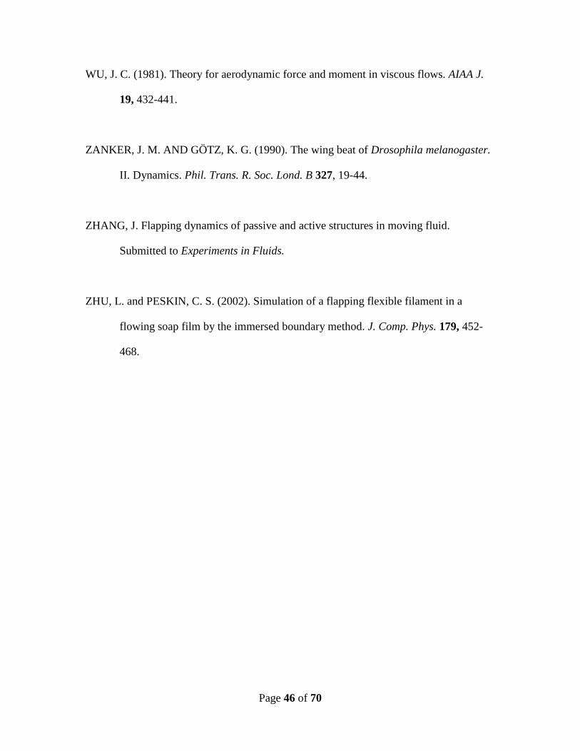
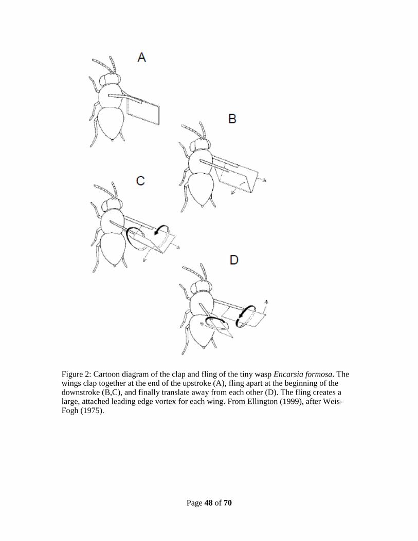
have been filmed to date appear to use ‘clap and fling’. Weis-Fogh (1973) first described
how the tiny wasp Encarsia formosa uses this motion and speculated that it augments the
lift forces generated by strengthening the bound vortex on each wing. The clap and fling
motion has also been reported in the greenhouse white-fly Trialeurodes vaporariorum
(Weis-Fogh, 1975) and Thrips physapus (Ellington, 1984a). The author has observed clap
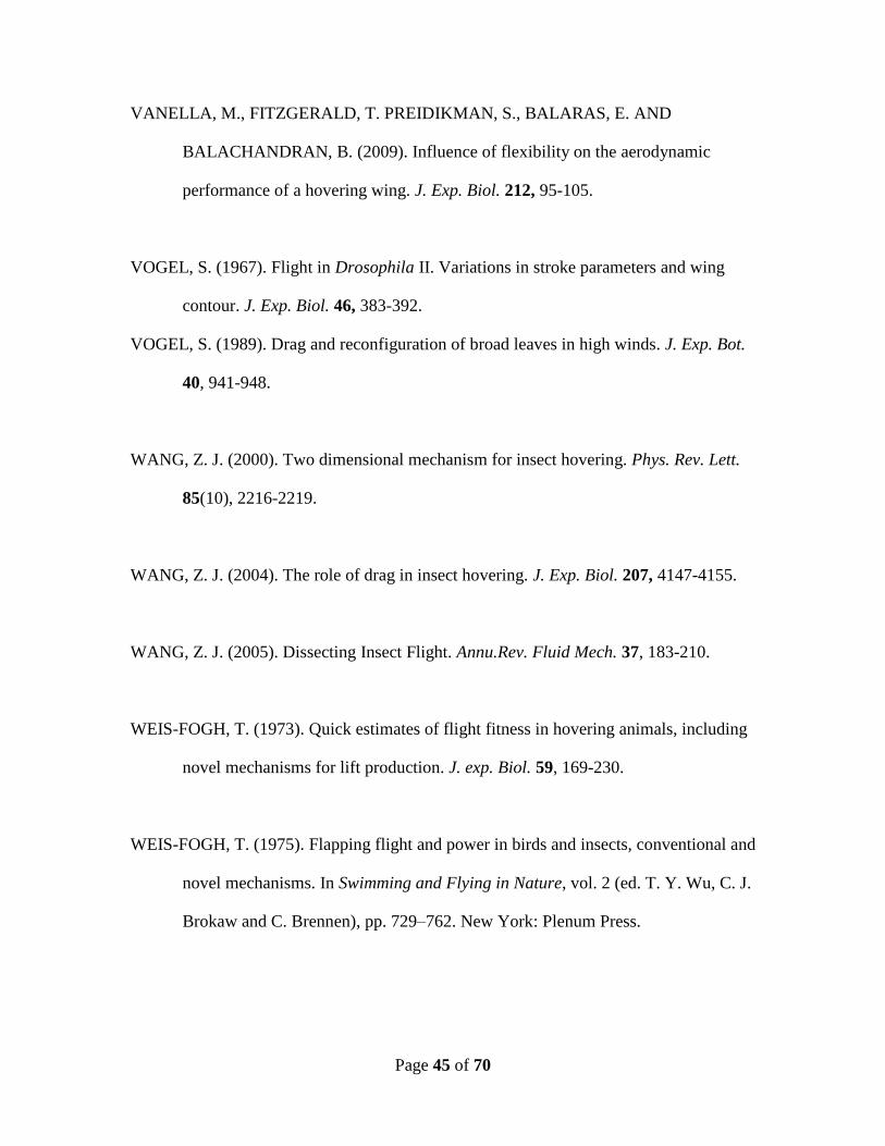
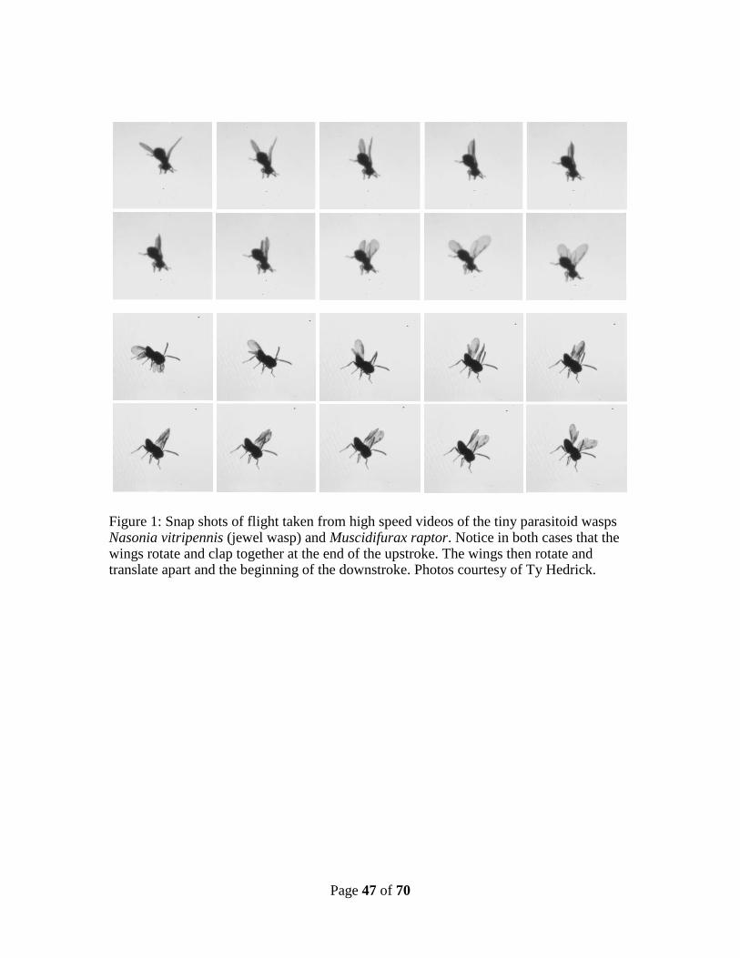
and fling kinematics in high speed videos of the tiny parasitoid wasps Muscidifurax
raptor and the jewel wasp Nasonia vitripennis (see Fig. 2). Fling has also been observed
Page 3 of 70
in a few medium and larger insects such as butterflies and moths (Marden, 1987) and the
tethered flight of Drosophila melanogaster (Vogel, 1967).
A combination of experimental, theoretical, and numerical work supports that insects
augment the lift forces generated during flight by the clap and fling mechanism
(Ellington, 1984a,b; Lehmann et al., 2005; Lehmann and Pick, 2007; Lighthill, 1973;
Miller and Peskin, 2005; Weis-Fogh, 1973). Lift is augmented during wing rotation
(fling) and subsequent translation by the formation of two large leading edge vortices
(Miller and Peskin, 2005; Sun and Xin, 2003). Much less attention has been given to the
total force required to actually clap the wings together and fling the wings apart. Miller
and Peskin (2005) found that relatively large forces are required to fling rigid wings apart
at Reynolds numbers below 20. Furthermore, the lift to drag ratios produced during clap
and fling are lower than the ratios for the corresponding one wing case, although the
absolute lift forces generated are larger. For the smallest insects, the forces required to
fling the wings are so large that it raises the question of why tiny insects clap and fling in
the first place.
One major assumption in previous clap and fling studies using physical models
(Lehmann et al., 2005; Lehmann and Pick, 2007; Maxworthy, 1979; Spedding and
Maxworthy, 1986; Sunada et al., 1993), mathematical models (Lighthill, 1973), and
numerical simulations (Chang and Sohn, 2006; Miller and Peskin, 2005; Sun and Xin,
2003) is that the wings are rigid. It seems likely that wing flexibility could allow the
wings to reconfigure to lower drag profiles during clap and fling. In this case, the fling
might appear more like a 'peel,' and the clap might be thought of as a reverse peel
Page 4 of 70
(Ellington, 1984a, 1984b). A number of studies support the idea that flexibility allows for
reconfiguration of biological structures, which results in reduced drag forces experienced
by the organisms (for example, Koehl, 1984; Vogel, 1989; Denny 1994; Etnier and
Vogel, 2000; Alben et al., 2002, 2004). The basic idea in these cases is that the force on
the body produced by the moving fluid causes the flexible body to bend or reconfigure
which, in turn, reduces the force felt by the body.
A number of recent computational and experimental studies have explored the role of
wing flexibility in augmenting aerodynamic performance in insects, but most of this work
has focused on single wings at ‘higher’ Reynolds numbers (>75). For example, Vanella et
al. (2009) explored the influence of flexibility on the lift to drag ratio for Reynolds
numbers ranging from 75 to 1000 using two-dimensional, two-link model of a single
wing. They found that aerodynamic performance was enhanced when the wing was
flapped at 1/3 of the natural frequency. Ishihara et al. (2009) studied passive pitching by
modeling a rigid wing that was free to pitch and were able to generate sinusoidal motions
that produced enough lift to support some Diptera. A number of other studies have
explored the role of wing flexibility in avian flight (Heathcote et al., 2008; Kim et al.,
2008) and thrust generation (Alben, 2008; Lauder et al., 2006; Mittal, 2006; Zhang,
submitted).
While flexibility will likely reduce the drag forces required for clap and fling, the wings
should not be so flexible that the lift forces produced are significantly diminished.
Ellington (1984b) suggested that a peel mechanism with flexible wings might actually
serve to augment lift forces relative to the rigid-fling case. In the case of peel, the wings
Page 5 of 70
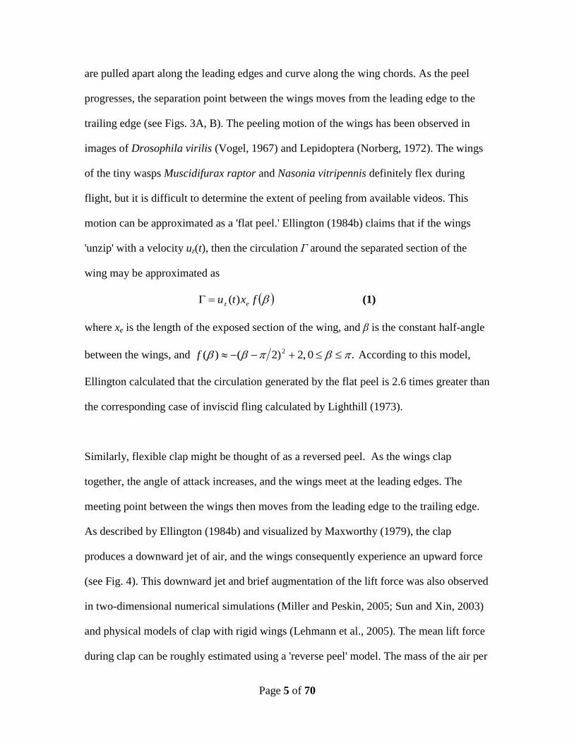
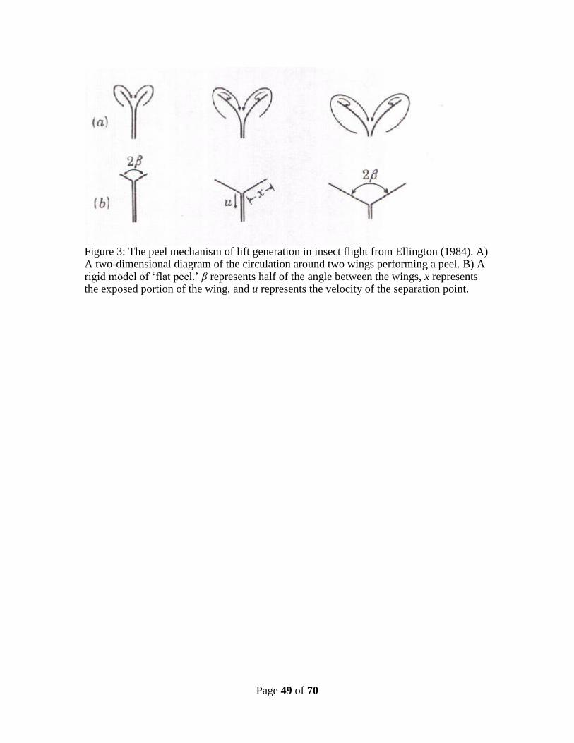
are pulled apart along the leading edges and curve along the wing chords. As the peel
progresses, the separation point between the wings moves from the leading edge to the
trailing edge (see Figs. 3A, B). The peeling motion of the wings has been observed in
images of Drosophila virilis (Vogel, 1967) and Lepidoptera (Norberg, 1972). The wings
of the tiny wasps Muscidifurax raptor and Nasonia vitripennis definitely flex during
flight, but it is difficult to determine the extent of peeling from available videos. This
motion can be approximated as a 'flat peel.' Ellington (1984b) claims that if the wings
'unzip' with a velocity uz(t), then the circulation Γ around the separated section of the
wing may be approximated as
(1) )( fxtu ez
where xe is the length of the exposed section of the wing, and β is the constant half-angle
between the wings, and .0 ,2)2()( 2 f According to this model,
Ellington calculated that the circulation generated by the flat peel is 2.6 times greater than
the corresponding case of inviscid fling calculated by Lighthill (1973).
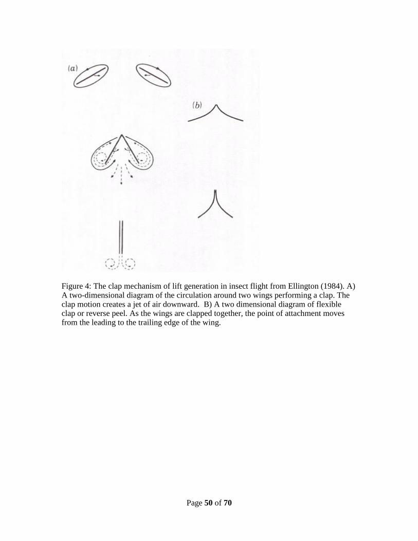
Similarly, flexible clap might be thought of as a reversed peel. As the wings clap
together, the angle of attack increases, and the wings meet at the leading edges. The
meeting point between the wings then moves from the leading edge to the trailing edge.
As described by Ellington (1984b) and visualized by Maxworthy (1979), the clap
produces a downward jet of air, and the wings consequently experience an upward force
(see Fig. 4). This downward jet and brief augmentation of the lift force was also observed
in two-dimensional numerical simulations (Miller and Peskin, 2005; Sun and Xin, 2003)
and physical models of clap with rigid wings (Lehmann et al., 2005). The mean lift force
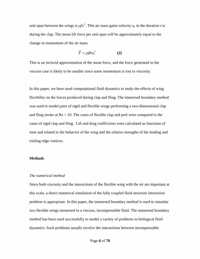
during clap can be roughly estimated using a 'reverse peel' model. The mass of the air per
Page 6 of 70
unit span between the wings is ρβc2. This air mass gains velocity uc in the duration c/u
during the clap. The mean lift force per unit span will be approximately equal to the
change in momentum of the air mass.
(2) 2
ccuF
This is an inviscid approximation of the mean force, and the force generated in the
viscous case is likely to be smaller since some momentum is lost to viscosity.
In this paper, we have used computational fluid dynamics to study the effects of wing
flexibility on the forces produced during clap and fling. The immersed boundary method
was used to model pairs of rigid and flexible wings performing a two-dimensional clap
and fling stroke at Re = 10. The cases of flexible clap and peel were compared to the
cases of rigid clap and fling. Lift and drag coefficients were calculated as functions of
time and related to the behavior of the wing and the relative strengths of the leading and
trailing edge vortices.
Methods
The numerical method
Since both viscosity and the interactions of the flexible wing with the air are important at
this scale, a direct numerical simulation of the fully coupled fluid-structure interaction
problem is appropriate. In this paper, the immersed boundary method is used to simulate
two flexible wings immersed in a viscous, incompressible fluid. The immersed boundary
method has been used successfully to model a variety of problems in biological fluid
dynamics. Such problems usually involve the interactions between incompressible
Page 7 of 70
viscous fluids and deformable elastic boundaries. Some examples of biological problems
that have been studied with the immersed boundary method include aquatic animal
locomotion (Fauci and Peskin, 1988; Fauci, 1990; Fauci and Fogelson, 1993), cardiac
blood flow (Kovacs, McQueen, and Peskin, 2001; McQueen and Peskin, 1997; McQueen
and Peskin, 2000; McQueen and Peskin, 2000), and ciliary driven flows (Grunbaum et
al., 1998).
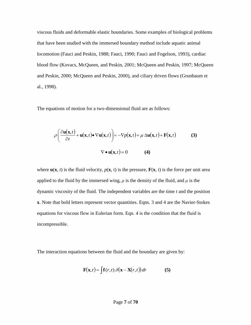
The equations of motion for a two-dimensional fluid are as follows:
(3)xFxuxxuxu
xu ,,,,,
,tttptt
t
t
(4) xu 0, t
where u(x, t) is the fluid velocity, p(x, t) is the pressure, F(x, t) is the force per unit area
applied to the fluid by the immersed wing, ρ is the density of the fluid, and μ is the
dynamic viscosity of the fluid. The independent variables are the time t and the position
x. Note that bold letters represent vector quantities. Eqns. 3 and 4 are the Navier-Stokes
equations for viscous flow in Eulerian form. Eqn. 4 is the condition that the fluid is
incompressible.
The interaction equations between the fluid and the boundary are given by:
(5) XxfxF ,),(, drtrtrt
Page 8 of 70
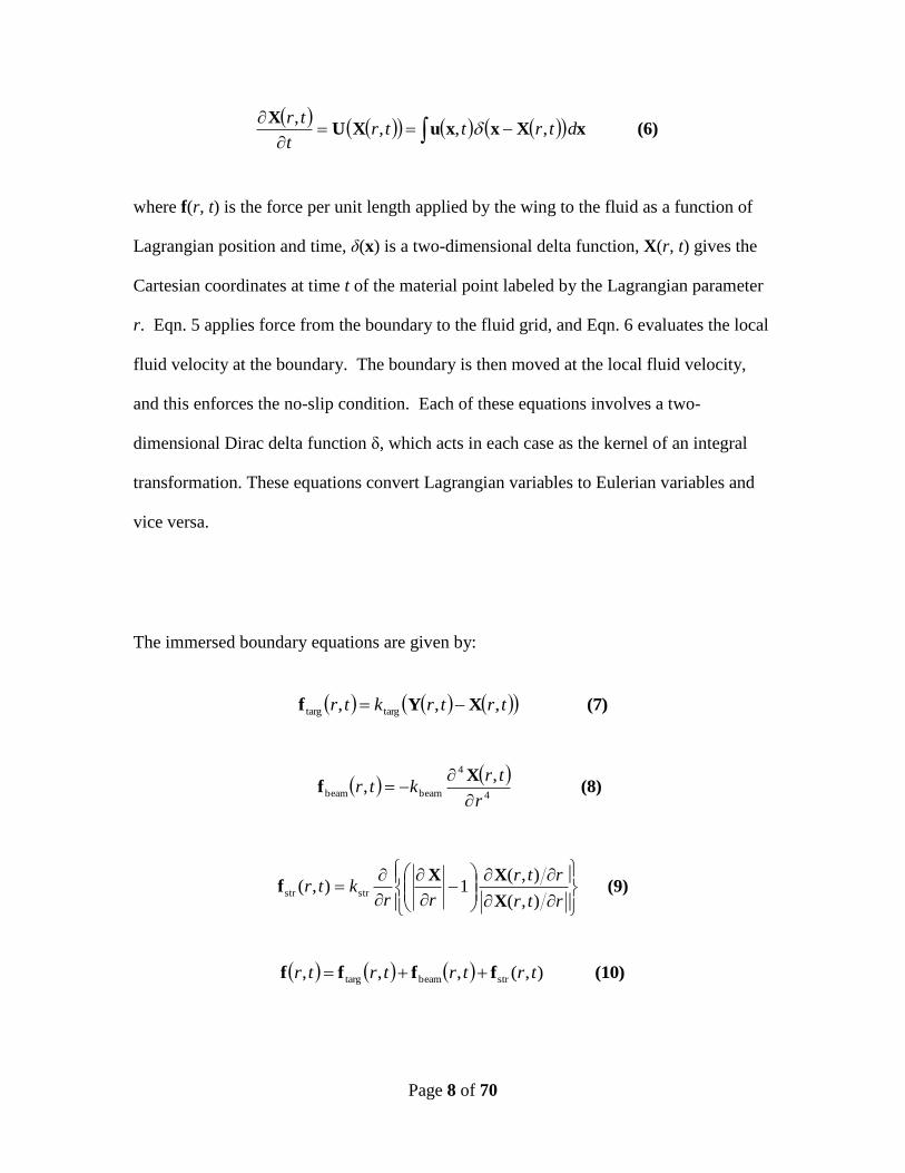
(6) xXxxuXU
X ,,,
,
dtrttr
t
tr
where f(r, t) is the force per unit length applied by the wing to the fluid as a function of
Lagrangian position and time, δ(x) is a two-dimensional delta function, X(r, t) gives the
Cartesian coordinates at time t of the material point labeled by the Lagrangian parameter
r. Eqn. 5 applies force from the boundary to the fluid grid, and Eqn. 6 evaluates the local
fluid velocity at the boundary. The boundary is then moved at the local fluid velocity,
and this enforces the no-slip condition. Each of these equations involves a two-
dimensional Dirac delta function δ, which acts in each case as the kernel of an integral
transformation. These equations convert Lagrangian variables to Eulerian variables and
vice versa.
The immersed boundary equations are given by:
(7) XYf ,,, targtarg trtrktr
(8) X
f ,
,4
4
beambeamr
trktr
(9)X
XXf
),(
),( 1),( strstr
rtr
rtr
rrktr
(10) ffff ),( ,,, strbeamtarg trtrtrtr
Page 9 of 70
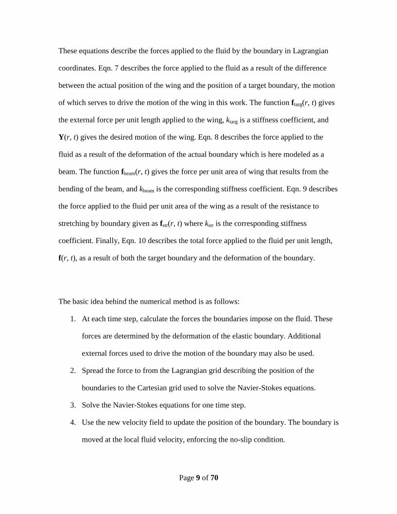
These equations describe the forces applied to the fluid by the boundary in Lagrangian
coordinates. Eqn. 7 describes the force applied to the fluid as a result of the difference
between the actual position of the wing and the position of a target boundary, the motion
of which serves to drive the motion of the wing in this work. The function ftarg(r, t) gives
the external force per unit length applied to the wing, ktarg is a stiffness coefficient, and
Y(r, t) gives the desired motion of the wing. Eqn. 8 describes the force applied to the
fluid as a result of the deformation of the actual boundary which is here modeled as a
beam. The function fbeam(r, t) gives the force per unit area of wing that results from the
bending of the beam, and kbeam is the corresponding stiffness coefficient. Eqn. 9 describes
the force applied to the fluid per unit area of the wing as a result of the resistance to
stretching by boundary given as fstr(r, t) where kstr is the corresponding stiffness
coefficient. Finally, Eqn. 10 describes the total force applied to the fluid per unit length,
f(r, t), as a result of both the target boundary and the deformation of the boundary.
The basic idea behind the numerical method is as follows:
1. At each time step, calculate the forces the boundaries impose on the fluid. These
forces are determined by the deformation of the elastic boundary. Additional
external forces used to drive the motion of the boundary may also be used.
2. Spread the force to from the Lagrangian grid describing the position of the
boundaries to the Cartesian grid used to solve the Navier-Stokes equations.
3. Solve the Navier-Stokes equations for one time step.
4. Use the new velocity field to update the position of the boundary. The boundary is
moved at the local fluid velocity, enforcing the no-slip condition.
Page 10 of 70
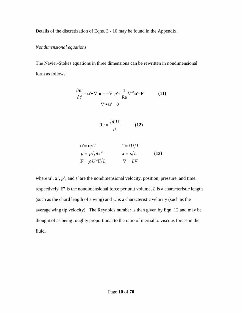
Details of the discretization of Eqns. 3 - 10 may be found in the Appendix.
Nondimensional equations
The Navier-Stokes equations in three dimensions can be rewritten in nondimensional
form as follows:
0u'
(11)Fuu'uu
'
'''Re
1''''
'
' 2pt
(12) Re
LU
LLU
LUpp
LUttU
' '
' '
' '
2
2
FF
(13)xx
uu
where u’, x’, p’, and t’ are the nondimensional velocity, position, pressure, and time,
respectively. F’ is the nondimensional force per unit volume, L is a characteristic length
(such as the chord length of a wing) and U is a characteristic velocity (such as the
average wing tip velocity). The Reynolds number is then given by Eqn. 12 and may be
thought of as being roughly proportional to the ratio of inertial to viscous forces in the
fluid.
Page 11 of 70
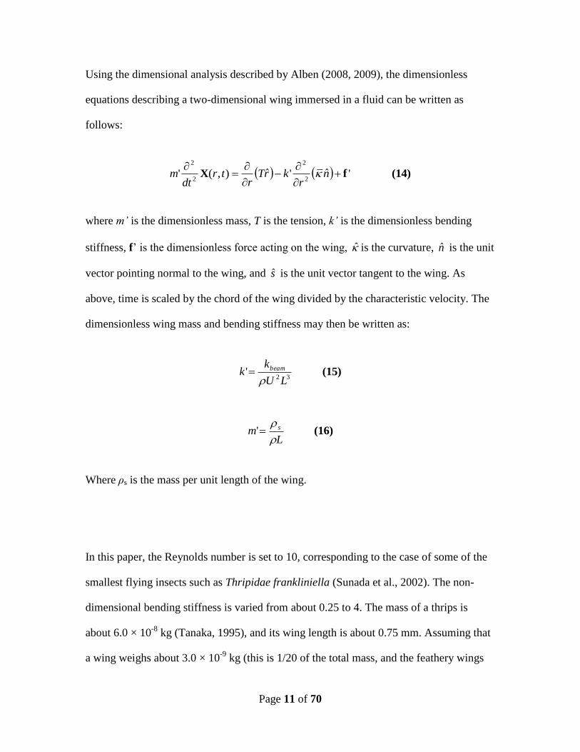
Using the dimensional analysis described by Alben (2008, 2009), the dimensionless
equations describing a two-dimensional wing immersed in a fluid can be written as
follows:
(14)fX 'ˆ'ˆ),('2
2
2
2
n
rkrT
rtr
dtm
where m’ is the dimensionless mass, T is the tension, k’ is the dimensionless bending
stiffness, f’ is the dimensionless force acting on the wing, is the curvature, n is the unit
vector pointing normal to the wing, and s is the unit vector tangent to the wing. As
above, time is scaled by the chord of the wing divided by the characteristic velocity. The
dimensionless wing mass and bending stiffness may then be written as:
(15) '32 LU
kk beam
(16) 'L
m s
Where ρs is the mass per unit length of the wing.
In this paper, the Reynolds number is set to 10, corresponding to the case of some of the
smallest flying insects such as Thripidae frankliniella (Sunada et al., 2002). The non-
dimensional bending stiffness is varied from about 0.25 to 4. The mass of a thrips is
about 6.0 × 10⁻⁸
kg (Tanaka, 1995), and its wing length is about 0.75 mm. Assuming that
a wing weighs about 3.0 × 10⁻⁹
kg (this is 1/20 of the total mass, and the feathery wings
Page 12 of 70
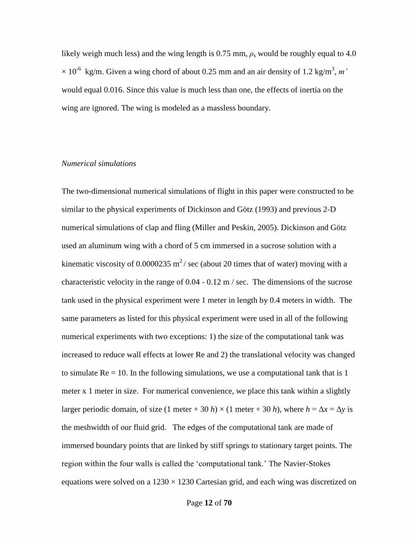
likely weigh much less) and the wing length is 0.75 mm, ρs would be roughly equal to 4.0
× 10-6
kg/m. Given a wing chord of about 0.25 mm and an air density of 1.2 kg/m3, m’
would equal 0.016. Since this value is much less than one, the effects of inertia on the
wing are ignored. The wing is modeled as a massless boundary.
Numerical simulations
The two-dimensional numerical simulations of flight in this paper were constructed to be
similar to the physical experiments of Dickinson and Götz (1993) and previous 2-D
numerical simulations of clap and fling (Miller and Peskin, 2005). Dickinson and Götz
used an aluminum wing with a chord of 5 cm immersed in a sucrose solution with a
kinematic viscosity of 0.0000235 m2
/ sec (about 20 times that of water) moving with a
characteristic velocity in the range of 0.04 - 0.12 m / sec. The dimensions of the sucrose
tank used in the physical experiment were 1 meter in length by 0.4 meters in width. The
same parameters as listed for this physical experiment were used in all of the following
numerical experiments with two exceptions: 1) the size of the computational tank was
increased to reduce wall effects at lower Re and 2) the translational velocity was changed
to simulate Re = 10. In the following simulations, we use a computational tank that is 1
meter x 1 meter in size. For numerical convenience, we place this tank within a slightly
larger periodic domain, of size (1 meter + 30 h) × (1 meter + 30 h), where h = Δx = Δy is
the meshwidth of our fluid grid. The edges of the computational tank are made of
immersed boundary points that are linked by stiff springs to stationary target points. The
region within the four walls is called the ‘computational tank.’ The Navier-Stokes
equations were solved on a 1230 × 1230 Cartesian grid, and each wing was discretized on
Page 13 of 70
a Lagrangian array of 60 points. Miller and Peskin (2005) presented a convergence
analysis that showed that this mesh size is within the range of convergence for the two
wing problem at Reynolds numbers below 100.
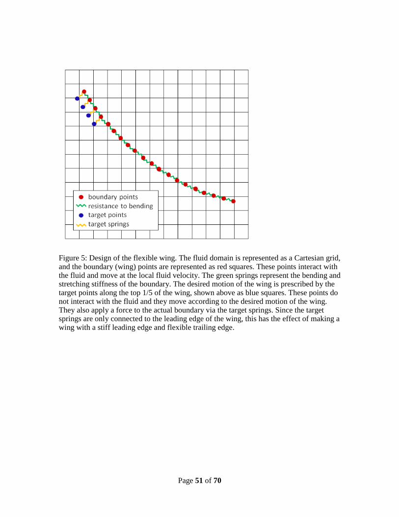
Unless otherwise stated, the motion of the flexible wings was prescribed by attaching
target points to the top fifth of the boundary along the leading edge of the wing with
springs (Fig. 5). The target points moved with the prescribed motion and applied a force
to the boundary proportional to the distance between the target and corresponding
boundary points. The bottom 4/5 of the wing (trailing edge) was free to bend. This has
the effect of modeling a flexible wing with a rigid leading edge. In the 'nearly-rigid' case,
springs were attached to target points along the entire length of the wing which prevented
any significant deformation. The stiffness coefficient of the springs that attach the
boundary points to the target points was ktarg = 1.44 105 kg / s
2, and the stiffness
coefficient for the tension or compression of the wing was also set to kstr = 1.44 105 kg /
s2. These values were chosen to prevent any significant stretching or deformation of the
wings in the rigid case.
The flexural or bending stiffness of the wing was varied from kbeam = 0.125 κ to 2 κ
2/ mN , where κ = 5.5459 610 2/ mN . As stated above, this range of bending stiffnesses
corresponds to nondimensional values ranging from 0.25 to 4. We chose this value of κ to
represent the case where deformations during translation are small, but bending does
occur when the wings are close. This range of values was found to produce deformations
that are qualitatively similar to those observed in flight videos.
Page 14 of 70
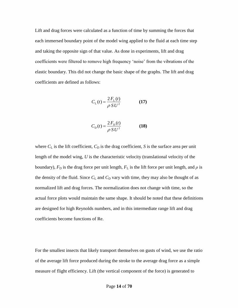
Lift and drag forces were calculated as a function of time by summing the forces that
each immersed boundary point of the model wing applied to the fluid at each time step
and taking the opposite sign of that value. As done in experiments, lift and drag
coefficients were filtered to remove high frequency ‘noise’ from the vibrations of the
elastic boundary. This did not change the basic shape of the graphs. The lift and drag
coefficients are defined as follows:
(17) )(2
)(2
LL
US
tFtC
(18) )(2
)(2
DD
US
tFtC
where CL is the lift coefficient, CD is the drag coefficient, S is the surface area per unit
length of the model wing, U is the characteristic velocity (translational velocity of the
boundary), FD is the drag force per unit length, FL is the lift force per unit length, and ρ is
the density of the fluid. Since CL and CD vary with time, they may also be thought of as
normalized lift and drag forces. The normalization does not change with time, so the
actual force plots would maintain the same shape. It should be noted that these definitions
are designed for high Reynolds numbers, and in this intermediate range lift and drag
coefficients become functions of Re.
For the smallest insects that likely transport themselves on gusts of wind, we use the ratio
of the average lift force produced during the stroke to the average drag force as a simple
measure of flight efficiency. Lift (the vertical component of the force) is generated to
Page 15 of 70
help keep the insects afloat while drag (the horizontal component of the force) is of less
importance since any thrust produced would likely be swamped by wind gusts. This
metric is particularly appropriate when the wings are close to each other since the
horizontal component of the force acting on each wing cancels. It is worthwhile to note
that many other measures of efficiency are used in the literature, many of which are likely
more appropriate for medium to large insects (see Wang, 2004, for example).
Kinematics of the clap and fling strokes
Quantitative descriptions of the wing beat kinematics of the smallest flying insects are
currently unavailable. This is partially due to the fact that these insects are extremely
difficult to film. Many of these insects may be as small as 0.25 mm in length and flap
their wings at frequencies of 200 Hz or greater (Dudley, 2000). The authors know of
several unpublished high speed videos of Thysanoptera, Muscidifurax raptor and
Nasonia vitripennis shot from a single camera, but quantitative reconstruction of the
wingbeat kinematics is not possible from one camera angle. The simplified flight
kinematics of clap and fling used in this paper are similar to those used by Lighthill
(1973), Bennett (1977), Maxworthy (1979), Spedding and Maxworthy (1986), Sun and
Xin (2003), Miller and Peskin (2005), and Chang and Sohn (2006) to investigate flight
aerodynamics using mathematical and physical models.
Either a single clap upstroke or a single fling downstroke was simulated. This
simplification was made since the influence of the wake produced by the previous stroke
Page 16 of 70
is small for Reynolds numbers of 10 and below. Chang and Sohn (2006) found changes
in the strength of the leading edge vortices at Reynolds numbers on the order of 100
when isolated clap and fling motions were compared to cyclical clap and fling motions,
but the overall aerodynamics and forces acting on the wings at Re = 10 were quite
similar.
At the end of the upstroke and the beginning of the downstroke, the wings were placed
1/10 chord lengths apart. This distance was chosen based on the analysis of Sun and Xin
(2003) who showed that the forces acting on the wings during clap and fling do not
change significantly for distances of 1/10 of the wing chord and lower. The kinematics of
the left wing during the clap strokes (upstrokes) are described here. The right wing (when
present) was the mirror image of the left wing at all times during its motion, and the
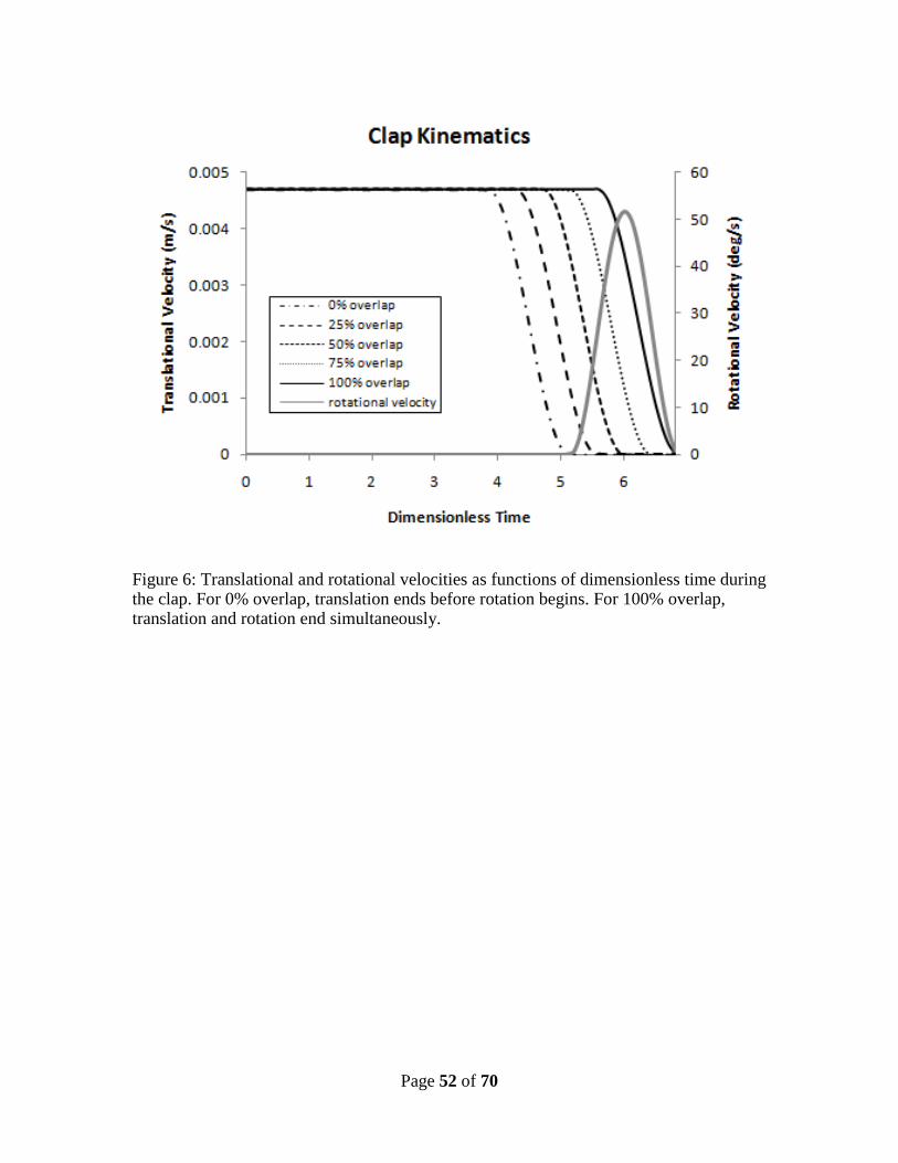
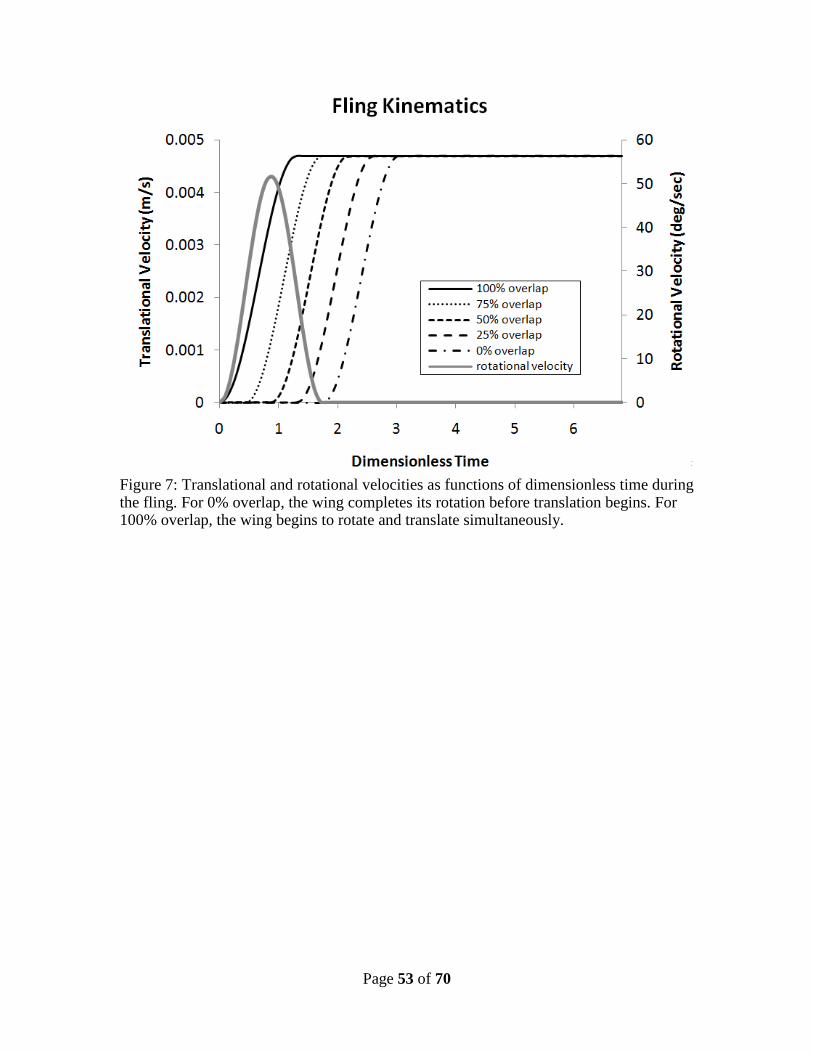
kinematics of the fling (downstroke) was symmetric to the upstroke. The translational
velocities during the clap stroke were constructed using a series of equations to describe
each part of the stroke. Plots of translational and angular velocities as functions of time
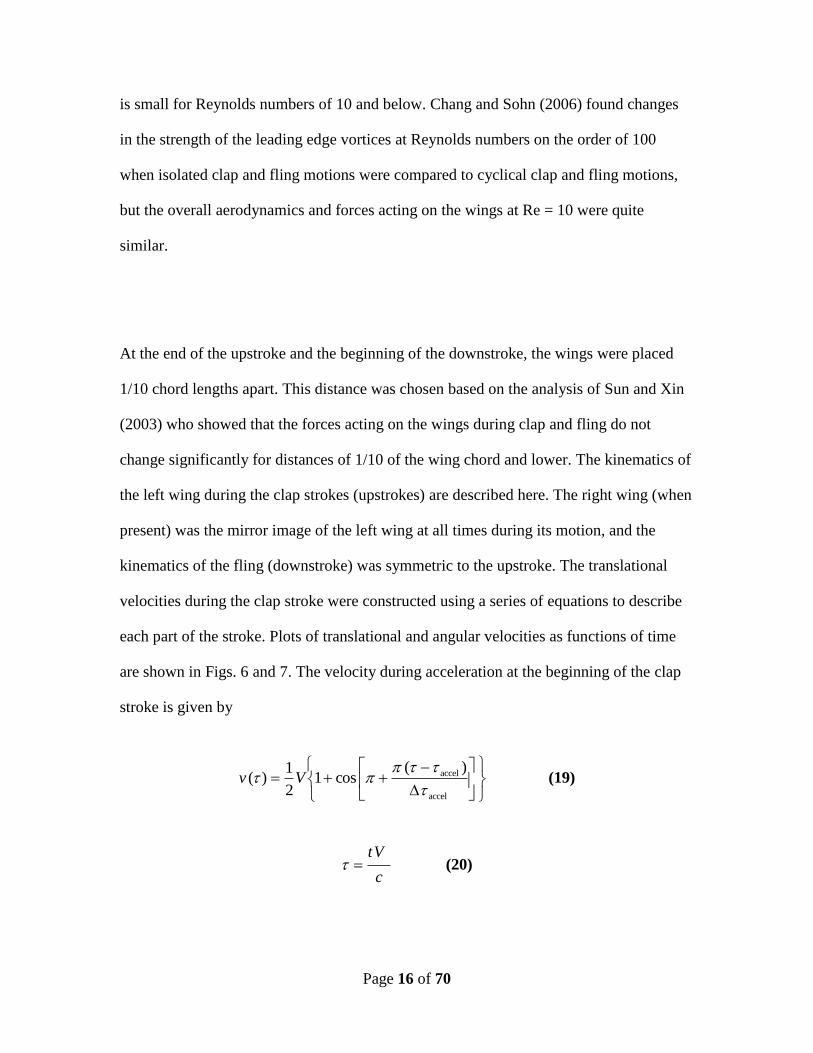
are shown in Figs. 6 and 7. The velocity during acceleration at the beginning of the clap
stroke is given by
(19) )(
cos12
1)(
accel
accel
Vv
(20) c
Vt
Page 17 of 70
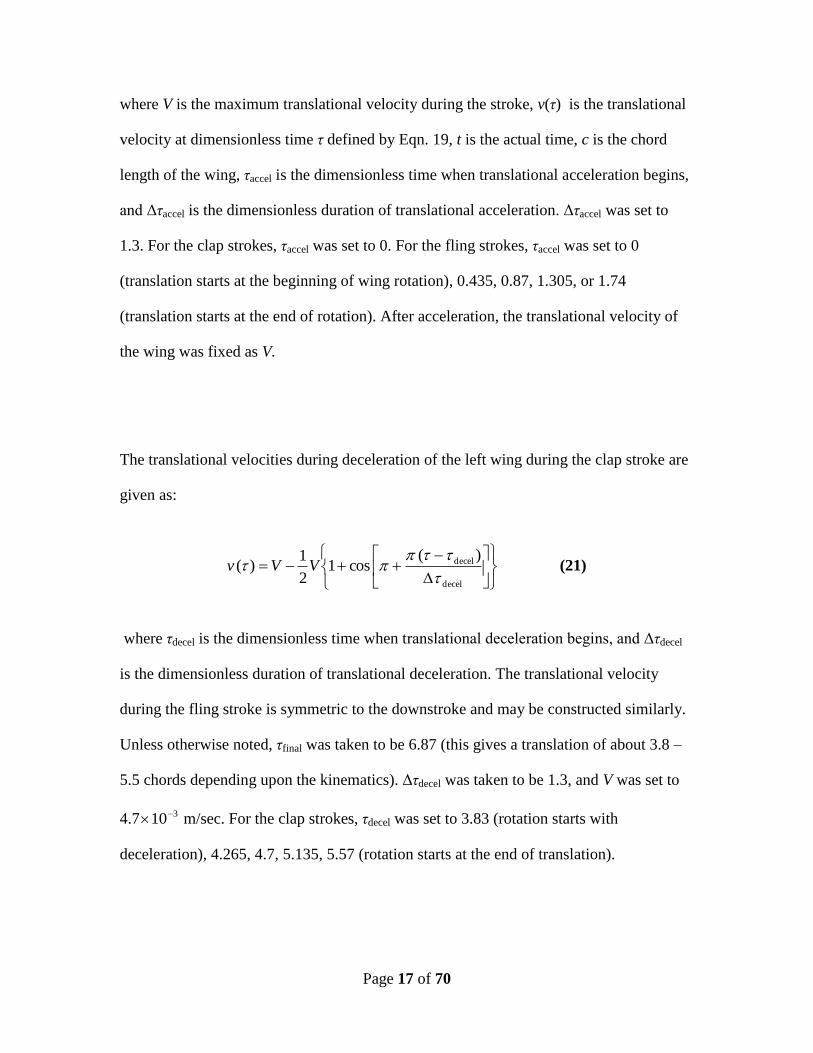
where V is the maximum translational velocity during the stroke, v(τ) is the translational
velocity at dimensionless time τ defined by Eqn. 19, t is the actual time, c is the chord
length of the wing, τaccel is the dimensionless time when translational acceleration begins,
and Δτaccel is the dimensionless duration of translational acceleration. Δτaccel was set to
1.3. For the clap strokes, τaccel was set to 0. For the fling strokes, τaccel was set to 0
(translation starts at the beginning of wing rotation), 0.435, 0.87, 1.305, or 1.74
(translation starts at the end of rotation). After acceleration, the translational velocity of
the wing was fixed as V.
The translational velocities during deceleration of the left wing during the clap stroke are
given as:
(21) )(
cos12
1)(
decel
decel
VVv
where τdecel is the dimensionless time when translational deceleration begins, and Δτdecel
is the dimensionless duration of translational deceleration. The translational velocity
during the fling stroke is symmetric to the downstroke and may be constructed similarly.
Unless otherwise noted, τfinal was taken to be 6.87 (this gives a translation of about 3.8 –
5.5 chords depending upon the kinematics). Δτdecel was taken to be 1.3, and V was set to
4.7 310 m/sec. For the clap strokes, τdecel was set to 3.83 (rotation starts with
deceleration), 4.265, 4.7, 5.135, 5.57 (rotation starts at the end of translation).
Page 18 of 70
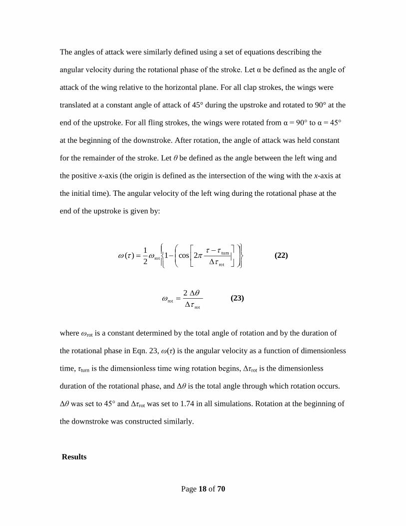
The angles of attack were similarly defined using a set of equations describing the
angular velocity during the rotational phase of the stroke. Let α be defined as the angle of
attack of the wing relative to the horizontal plane. For all clap strokes, the wings were
translated at a constant angle of attack of 45° during the upstroke and rotated to 90° at the
end of the upstroke. For all fling strokes, the wings were rotated from α = 90° to α = 45°
at the beginning of the downstroke. After rotation, the angle of attack was held constant
for the remainder of the stroke. Let θ be defined as the angle between the left wing and
the positive x-axis (the origin is defined as the intersection of the wing with the x-axis at
the initial time). The angular velocity of the left wing during the rotational phase at the
end of the upstroke is given by:
(22) 2cos12
1)(
rot
turn
rot
(23) 2
rot
rot
where ωrot is a constant determined by the total angle of rotation and by the duration of
the rotational phase in Eqn. 23, ω(τ) is the angular velocity as a function of dimensionless
time, τturn is the dimensionless time wing rotation begins, Δτrot is the dimensionless
duration of the rotational phase, and Δθ is the total angle through which rotation occurs.
Δθ was set to 45° and Δτrot was set to 1.74 in all simulations. Rotation at the beginning of
the downstroke was constructed similarly.
Results
Page 19 of 70
Translational/Rotational Overlap
For this set of simulations, we vary the translational-rotational overlap during wing
rotation for clap and fling strokes and considered nearly-rigid and flexible wings (kbeam =
κ). For the clap simulations, the wings come to rest at the beginning, first quarter, middle,
third quarter, or end of rotation. This corresponds to 0, 0.25, 0.5, 0.75, and 1.0 overlap
between rotation and translation (τdecel = 3.83, 4.265, 4.7, 5.135, and 5.57). For the fling
simulations, translation begins at the beginning, first quarter, middle, third quarter, or end
of rotation. Similarly, this corresponds to 1.0, 0.75, 0.5, 0.25, and 0 overlap between
rotation and translation (τaccel = 0, 0.435, 0.87, 1.305, or 1.74).
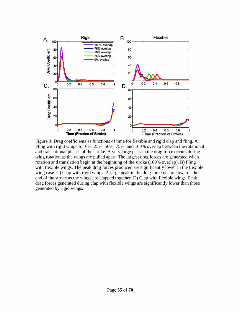
Lift coefficients and drag coefficients as functions of time (expressed as the fraction of
the stroke) for the four cases (rigid clap, rigid fling, flexible clap, and flexible fling) are
shown in Figs. 8 and 9. For the clap strokes, the first peak in the force coefficients
corresponds to the acceleration of the wing from rest. The force coefficients quickly
reach steady values until the wings begin to decelerate and rotate. The next peak in the
force coefficients corresponds to the rotation of the wings together (clap). Large lift and
drag forces are produced as the air between the wings is squeezed downward. Note that
lift coefficients produced during the rigid and flexible clap strokes are comparable, but
the maximum drag coefficients produced during the clap are significantly lower in the
flexible case.
For the fling strokes, the first peak in the force coefficients corresponds to the rotation of
the wings apart (fling). The peak lift forces in the flexible cases are higher than in the
Page 20 of 70
corresponding rigid cases. There are several possible explanations for this phenomenon.
Peel delays the formation of the trailing edge vortices, thereby maintaining vortical
asymmetry and augmenting lift for longer periods (Miller and Peskin, 2005). Similarly,
the suppression of the formation of the trailing edge vortex would also reduce the Wagner
effect at the beginning of translation (Weis-Fogh, 1973). Lift augmentation by ‘peel’
verses ‘fling’ was also predicted using simple analytic models of inviscid flows around
rigid wings (Ellington, 1984b). As the wings are peeled apart, the wings are deformed
and store elastic energy. As the wings translate apart, the wings ‘straighten’ and push
down on the fluid, causing an upwards lift force. Not only is the lift greater, but the drag
is also lower in the flexible case, thus further enhancing the advantage of a flexible wing.
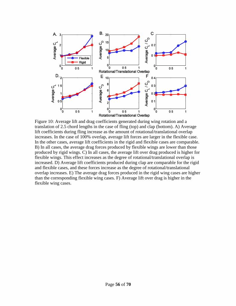
For a comparison of the average forces generated in each case, lift and drag coefficients
were averaged over wing rotation and 2.5 chord lengths of travel as shown in Fig. 10.
Please note that this is equivalent to take the ratio of the average lift force to the average
drag force produced. For the fling cases, average lift coefficients increase as the amount
of rotational/translational overlap increases. In the case of 100% overlap, average lift
forces are larger in the flexible case than in the rigid case. For other degrees of overlap,
average lift coefficients for rigid and flexible wings are comparable. For all overlaping
fling cases, the average drag coefficients produced by flexible wings are lower than those
produced by rigid wings. Moreover, the average ratio of lift to drag produced during fling
is higher for flexible wings than for rigid wings. This effect increases as the degree of
rotational/translational overlap is increased. For the clap cases, average lift coefficients
are comparable for rigid and flexible wings, and these forces increase as the degree of
rotational/translational overlap increases. The average drag forces produced in the rigid
Page 21 of 70
wing cases, however, are higher than the corresponding flexible wing cases. As a result,
average lift over drag is higher for flexible wings. In summary, these results suggest that
wing flexibility could improve the efficiency of hovering flight at low Re.
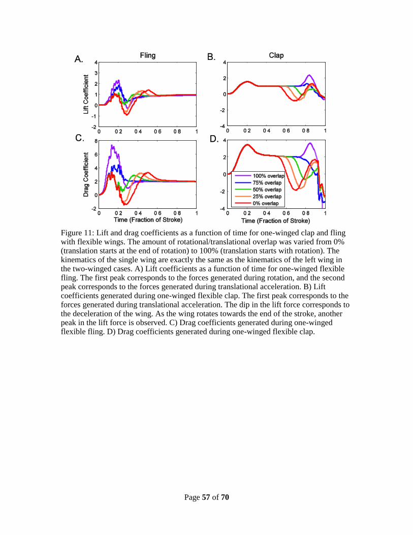
In order to answer the age-old question, what is the sound of one wing clapping, we now
consider a single wing moving according to the same kinematics as in the two-wing case.
The force coefficients as functions of time are shown in Fig. 11. During the fling motion,
the first peak in the force coefficients corresponds to the forces generated during rotation,
and the second peak corresponds to the forces generated during translational acceleration.
Wing deformation during one-winged clap and fling is minimal, and these force traces
are similar to the rigid wing case (data not shown). By comparing the scale bar between
Figs. 9 and 11, one can easily see the that maximum drag forces generated during two-
winged fling are 10 times higher than the maximum generated by one wing (either rigid
or flexible). During the clap motion, the first peak in the force coefficients corresponds to
the forces generated during translational acceleration. The first dip in the force
coefficients towards the end of the stroke corresponds to the deceleration of the wing. As
the wing rotates towards the end of the stroke, another peak in the lift and drag forces
force is observed. These forces quickly drop as the wing decelerates to rest. Force
coefficients for one-winged clap and fling averaged over rotation and 2.5 chord lengths of
translation are shown in Fig. 12.
Streamline plots of the fluid flow around wings performing a fling with 100% overlap
between the translational and rotational phases are shown in Fig. 13. The streamlines are
Page 22 of 70
curves which have the same direction as the instantaneous fluid velocity u(x, t) at each
point. They were drawn by making a contour map of the stream function since the stream
function is constant along streamlines. The stream function ψ(x, t) in 2-D is defined by
the following equations:
(24)x
xx
x ,
, ,
,x
ttv
y
ttu
where u(x, t) and v(x, t) are components of the fluid velocity u(x, t) = [u(x, t), v(x, t)].
The density of the streamlines is proportional to the speed of the flow. Color has been
added to the streamline plots to help the reader distinguish individual streamlines and
vortices. Regions of negative vorticity appear as warm colors and positive vorticity
appear as cool colors. Close up views of the deformation of the left wing for each case at
four points in time are shown in Fig. 14.
Two-winged fling with rigid wings is shown in Fig. 13A. During wing rotation, two large
leading edge vortices begin to form as the wings fling apart (i-ii). As translation begins, a
pair of trailing edge vortices forms and begins to grow in strength (ii – iv). Two-winged
fling with flexible wings (kbeam = κ) is shown in Fig. 13B. The wings move with the same
motion as in 13A (100% rotational/translational overlap). As the wings move apart, the
point of separation moves from the leading edge to the trailing edge of the wing (i-ii).
The formation of the trailing edge vortices occurs later in the stroke, and the trailing edge
vortices are relatively weaker than the rigid wing case (ii–iv). One flexible wing (kbeam =
κ) moving with the same fling motion as A and B is shown in Fig. 13C. Because of the
Page 23 of 70
smaller aerodynamic forces acting on the wing, its deformation is negligible and is very
close to the rigid wing case (Fig. 14).
Streamline plots of the flow around wings performing a clap with 100% overlap between
the translational and rotational phases are shown in Fig. 15. Two-winged clap with rigid
wings is shown in 15A. As the wings clap together, the fluid is pushed out between the
trailing edges causing an upwards lift force (i-iv). Two-winged clap with flexible wings
(kbeam = κ) using the same motion is shown in 15B. Towards the end of the stroke, the
wings bend as they are clapped together, reducing the peak drag forces generated (ii-iv).
In addition, the point of ‘attachment’ moves from the leading edge to the trailing edge of
the wing. One flexible wing (kbeam = κ) moving with the same clap motion is shown in
15C. Because of the smaller aerodynamic forces acting on the wing, its deformation is
negligible.
Varying wing flexibilities
In this set of simulations, the flexural stiffness of the wings was varied from 0.25 κ to 2 κ,
and the translational/rotational during clap and fling overlap was set to 100%. The lift
and drag coefficients for clap and fling cases are shown in Fig 16. Lift coefficients as
functions of dimensionless time during two-winged flexible fling are shown in 16A. The
largest lift forces are produced for the case where kbeam = 1.25κ. Lift coefficients decrease
as the bending stiffness of the wing increases or decreases from this value. Lift
coefficients generated during two-winged flexible clap are shown in 15B. The lift
coefficients are comparable for all five values of the bending stiffness. Drag coefficients
Page 24 of 70
generated during two-winged flexible fling are shown in 15C. For this range of values,
the drag coefficients increase with increasing bending stiffness. Drag coefficients
generated during two-winged flexible clap are shown in 15D. Drag coefficients also
increase with increasing bending stiffness for this range of values.
Average lift and drag during wing rotation and a 2.5 chord translation are shown in Fig.
16. Average lift coefficients for flexible clap and fling are shown in Fig. 16A. The
average lift coefficient generated during fling was greatest when the bending stiffness
was set to 1.25 κ. The average lift generated during clap was relatively constant for this
range of values. The average drag coefficients for flexible clap and fling are shown in
16B. For the both clap and fling, the average drag coefficients increase with increasing
bending stiffness. Average lift over drag ratios for flexible clap and fling are shown in
16C. Lift over drag increases with decreasing bending stiffness.
Varying the rigid section of the wing
To investigate the effect of wing stiffness asymmetries on the forces produced during
flight, the rigid section of the flexible wing (1/5 of the chord length) was moved from the
leading to the trailing edge of the wing in five steps. In all cases, the flexural stiffness of
the wings was set to 1.0κ. The rotational/translational overlap was set to 100%. Combes
and Daniels (2003) measured the flexural stiffness of Manduca sexta wings as a function
of distance along the chord and found that the bending stiffness decreases from the
leading to the trailing edge of the wing. A quick look at the wing morphology of most
insect wings suggests that this is true for many species, making the assumption that
flexural stiffness is proportional to wing thickness. There might be a few exceptions to
Page 25 of 70
this rule, however. For example, if the bristles of thrips’ wings are more flexible than the
solid portion, then there may be some variation in the location of the stiffest portion of
the wing as a function of distance from the leading to the trailing edge.
Lift coefficients and drag coefficients as functions of time (expressed as the fraction of
the stroke) for clap and fling with the various wing designs are shown in Fig. 18. In all
cases, the rotational/translational overlap was set to 100% and the flexural stiffness of the
wing was set to kbeam = κ. The rigid portion of the wing was also the location where the
external force used to move the wing was applied. Lift coefficients during flexible fling
are shown in 18A. The largest lift forces were produced in the case where the middle of
the wing was made rigid. The smallest lift forces where produced in the case where the
trailing edge of the wing was rigid. Lift coefficients generated during flexible clap are
shown in 18B. The lift forces produced for all wing designs are comparable. Drag
coefficients generated during flexible fling are shown in 18C. The largest drag forces
were produced when the middle portion of the wing was rigid. These forces are
significantly larger than all other cases. Drag coefficients generated during flexible clap
are shown in 18D. The smallest peak drag forces were produced when the leading edge of
the wing was rigid.
Average lift and drag coefficients during rotation and a 2.5 chord translation are shown in
Fig. 19. Average lift coefficients as a function of the wing design (location of the rigid
portion of the wing) for flexible clap and fling are shown in 19A.The average lift
coefficient generated during fling was greatest when the middle part of the wing was
rigid. The lowest lift forces were generated when the trailing edge of the wing was rigid.
Page 26 of 70
The average lift generated during clap was relatively constant for each wing design.
Average drag coefficients are shown in 19B. In the case of fling, the largest average drag
coefficients were generated when the middle part of the wing was rigid. These forces
dropped as the rigid part was moved to either the leading or trailing edge of the wing. In
the case of clap, the forces generated were relatively constant. Average lift over drag for
clap and fling as a function of the location of the rigid part of the wing are shown in 19C.
Average lift over drag increases as the rigid part is moved towards the leading edge of the
wing.
Streamline plots of the flow around wings during fling for three wing designs are shown
in Fig 20, and plots of the wing configurations at three points in time are shown in figure
21. The flow around two wings designed so that the rigid part of the wing is along the
leading edge is shown in 20A. Two large leading edge vortices begin to form as the
wings fling apart (i-ii). As translation begins, a pair of trailing edge vortices forms and
begins to grow in strength (ii–iv). The flow around two wings where the rigid part is in
the middle of the wing is shown in 20B. As the wings are pulled apart, large deformations
of the wings occur along the leading and trailing edges (Fig 21 ii). When the leading and
trailing edges separate, large leading edge vortices are formed (ii-iv). The flow around
two wings where the rigid part of the wing is along the trailing edge is shown in 20C. As
the wings move apart, the point of separation moves from the trailing to the leading edge
of the wing. Large trailing edge vortices are formed at the beginning of the stroke, and
the leading edge vortices are small.
Page 27 of 70
Streamline plots of the flow around wings performing clap with three different wing
designs are shown in Fig. 22. Flow around two wings where the rigid part of the wing is
along the leading edge is shown in 22A. Towards the end of the stroke, the wings bend as
they are clapped together, reducing the peak drag generated. Flow around two wings
where the rigid part of the wing is in the middle of the wing is shown in 22B. This case is
similar to the rigid wing case since wing deformations are minimal. Flow around two
wings where the rigid part of the wing is at the trailing edge is shown in 22C. This case is
also similar to the rigid wing case since wing deformations are minimal.
Discussion
The results of this study suggest that wing flexibility may be important for reducing drag
forces generated during clap and fling at low Reynolds numbers, and some lift
augmenting effects may also be produced. This is significant since the drag forces
generated during 2-wing fling may be as much as 10 times higher than those generated
for one wing moving with the same motion. For flexible wings, the fling part of the
stroke is more like a peel, and the clap part of the stroke is more like a reverse peel.
When wing translation begins with wing rotation (100% overlap), lift forces are higher
for flexible wings. As the wings peel apart, the point of separation travels from the
leading to the trailing edge of the wing. This delays the formation of the trailing edge
vortices, which reduces the Wagner effect and sustains vortical asymmetry (large leading
edge vortex and small trailing edge vortex) for a larger portion of the stroke (please see
the discussion below). Increased lift production by wing peel vs. fling was also predicted
by Ellington (1984b).
Page 28 of 70
Asymmetries in flexural stiffness along the wing chord also influence aerodynamic
performance. Wings that are more rigid along the trailing edge of the wing maximize the
average lift/drag forces produced during fling. Wings that are more rigid in the middle
maximize the average lift force produced during fling. This result suggests that
differences in wing design could reflect different performance parameters that an insect
has ‘maximized.’
Average lift forces were greatest during fling when the flexural stiffness of the wing was
set to kbeam = 1.25κ. Using this value for the flexural stiffness of the wings, deformations
during translation or single wing flapping are minimal, and the force coefficients
produced are comparable to the rigid wing case. These results agree with the qualitative
observations of Ellington (1980) who oscillated single thrips’ wings at the frequency and
amplitude characteristic of flight. Since the forces generated during the clap and fling
portion of the strokes are so much larger than the single wing case because of wing-wing
interactions, wing deformations in the numerical simulations presented in this paper are
significant and greatly influence the aerodynamics. Measurements of the actual flexural
stiffness of tiny insect wings and experimental work that considers wing-wing
interactions at low Re are needed to verify this effect.
Relating the wake to the forces generated
To understand the aerodynamic mechanisms of lift and drag generation, we apply the
general aerodynamic theory for viscous flows presented by Wu (1981). For the particular
case of fling shown in Fig 23, assume two wings were rotated apart along their trailing
Page 29 of 70
edges and are now translating away from each other along a horizontal plane. During
rotation, two large leading edge vortices (Rn1 and Rp1) of equal strength and opposite
sign were formed and remain attached to the wing. During translation, two small trailing
edge vortices of equal strength and opposite sign begin to form and grow in strength (Rn2
and Rp2). Let the rest of the fluid domain Rf be of negligible vorticity. Note that the
subscript n denotes regions of negative (clockwise) vorticity, and p denotes regions of
positive (counterclockwise) vorticity. In the following discussion, an Eulerian frame of
reference will be used. The total lift acting on both wings can then be defined as follows
(Miller and Peskin, 2005):
(25)f nnppR 2R1R2R1R
dydxx
dt
ddydxx
dt
ddydxx
dt
dFL
where is the absolute value of the vorticity. The vortices in each pair are convected in
opposite directions with each wing as the wings are translated apart. The vortices defined
by Rn1 and Rp2 move with negative velocity. The vortices defined by Rp1 and Rn2 move
with positive velocity. The equation for total lift in this case can be rewritten as follows:
(26)2R2R
1R1R
pn
pn
dydxxdt
ddydxx
dt
d
dydxxdt
ddydxx
dt
dFL
This equation basically states that the total lift on both wings is proportional to the
difference between the magnitude of the time rate of change of the first moment of
vorticity associated with the leading edge vorticity and the time rate of change of the first
moment of trailing edge vorticity. Therefore, suppression of the formation of the trailing
edge vortex from the motion of the peel should transiently enhance lift forces during
translation.
Page 30 of 70
To understand the aerodynamic mechanism of drag generation, consider the case of a
wing in translation as shown in Fig 24. Both wings are started from rest and are now
translating at a constant velocity. The Reynolds number of the wing in (A) is larger than
that of (B), but both wings translate at Re < 30 (this prevents the separation of the trailing
edge vortex). During translation, a leading edge vortex (Rn) and a trailing edge vortex
(Rp) of equal strength and opposite sign were formed and remain attached to the wing.
Let the rest of the fluid domain Rf be of negligible vorticity. As above, the subscript n
denotes regions of negative (clockwise) vorticity, and p denotes regions of positive
(counterclockwise) vorticity. The vortices formed are more diffuse for the lower
Reynolds number. The total drag force acting on both wings can then be defined as
follows:
f pnR RR
(27) dydxydt
ddydxy
dt
ddydxy
dt
dFD
This equation basically states that increasing the time rate of change of vorticity in the y-
direction increases the relative drag forces generated. In other words, larger vortices that
move away from the wing in the vertical direction generate larger drag forces than
compact vortices.
Limitations of the model
Although the lift forces generated for flexible clap and fling using the particular wing
kinematics described in this paper are in some cases larger than the corresponding lift
forces generated for the rigid wing, one cannot extend these results to flexible wings in
Page 31 of 70
general. In fact, a flexible single wing using the same motion generates lower lift than a
rigid wing. Since the wing kinematics studied in this paper do not represent the optimal
case, it is not necessarily true that the optimal flexible wing stroke would outperform the
optimal rigid wing stroke. What can be concluded from this work is that 1) the drag
forces generated from wing-wing interactions can be an order of magnitude larger than a
single wing, and 2) the addition of flexibility can reduce the drag, but the maximum and
average drag forces are still substantially larger than the single wing case.
Ideally, one would like to be able to explore a wide parameter space of wing beat
kinematics and find the optimal rigid and flexible wing strokes, similar to the studies
presented by Berman and Wang (2007) for rigid wings and Alben (2008) for flexible
appendages. Unfortunately, one cannot make the quasi steady or inviscid assumptions at
Re = 10 to make this sort of analysis feasible. It may be possible to determine optimal
rigid and flexible wing strokes with the use of physical models, but new custom
experimental systems will need to be designed to measure the small forces generated by
flapping appendages at this scale.
Implications for bristled wings
Although wing flexibility reduces the amount of force needed to clap the wings together
and fling them apart, these forces are still significantly larger than the forces generated
during single-wing translation. In addition, lift over drag ratios are lower for two-winged
clap and fling than for one-winged translation. It could be the case that tiny insects
sacrifice aerodynamic efficiency for increased lift. Another possibility for some tiny
insects is that wing fringing further reduces the force required to clap the wings together
Page 32 of 70
and fling the wings apart. During wing rotation in the clap and fling, there could be some
flow between the wings’ bristles which would reduce the aerodynamic forces generated.
If the spacing of the bristles and the Reynolds number is near the transition where the
bristled appendages act either as leaky rakes or solid paddles (Cheer and Koehl, 1987),
then it could be possible for the wings to act as solid plates during translation. This might
allow for lift to be preserved during flight.
Acknowledgements
The authors would like to thank Ty Hedrick for the snap shots of Muscidifurax raptor
and Nasonia vitripennis used in this paper. The work was funded by Miller’s Burroughs
Wellcome Fund Career Award at the Scientific Interface.
Appendix
The system of differentio-integral equations given by Eqns. 3 – 10 was solved on a
square grid with periodic boundary conditions. The Navier-Stokes equations were
discretized on a fixed Cartesian grid, and the wings were discretized on a moving
Lagrangian array of points. Consider the discretization of the equations that describe the
force applied to the fluid as a result of the deformation of the boundary (Eqns. 7 – 10).
Let Δt be the duration of the time step, let Δr be the length of a boundary spatial step, let
n be the time step index, and let r define the location of a boundary point in the
Lagrangian framework (r = mΔr, m is an integer). Also, let Xn(r) = X(r, nΔt), Y
n(r) =
Y(r, nΔt), un(x) = u(x, nΔt), and p
n(x) = p(x, nΔt). For any function (r), let (Dr )(r) be
defined by the following equation:
Page 33 of 70
(A.1) 22
r
rr
rr
rDr
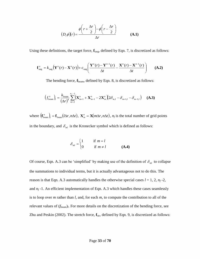
Using these definitions, the target force, ftarg, defined by Eqn. 7, is discretized as follows:
(A.2)XXYY
XYf )()()()(
)()(11
targtargtarg
t
rr
t
rrcrrk
nnnnnnn
The bending force, fbeam, defined by Eqn. 8, is discretized as follows:
(A.3)XXX 22 ,1,1,
1
2
114
beam
beam lmlmlm
n
m
n
m
n
m
n
ml
nf
r
kf
where tnrll
n ,beambeam ff , tnrmn
m ,XX , nf is the total number of grid points
in the boundary, and ml is the Kronecker symbol which is defined as follows:
(A.4) if 0
if 1
lm
lmml
Of course, Eqn. A.3 can be ‘simplified’ by making use of the definition of ml to collapse
the summations to individual terms, but it is actually advantageous not to do this. The
reason is that Eqn. A.3 automatically handles the otherwise special cases l = 1, 2, nf -2,
and nf -1. An efficient implementation of Eqn. A.3 which handles these cases seamlessly
is to loop over m rather than l, and, for each m, to compute the contribution to all of the
relevant values of (fbeam)l. For more details on the discretization of the bending force, see
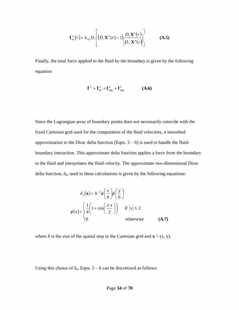
Zhu and Peskin (2002). The stretch force, fstr, defined by Eqn. 9, is discretized as follows:
Page 34 of 70
(A.5)
X
XXf 1)(strstr
rD
rDrDDkr
n
r
n
rn
rr
n
Finally, the total force applied to the fluid by the boundary is given by the following
equation:
(A.6) ffff targtargstr
nnnn
Since the Lagrangian array of boundary points does not necessarily coincide with the
fixed Cartesian grid used for the computation of the fluid velocities, a smoothed
approximation to the Dirac delta function (Eqns. 5 – 6) is used to handle the fluid-
boundary interaction. This approximate delta function applies a force from the boundary
to the fluid and interpolates the fluid velocity. The approximate two-dimensional Dirac
delta function, δh, used in these calculations is given by the following equations:
(A.7)
x
otherwise 0
2 if 2
cos14
1
2
ss
s
h
y
h
xhh
where h is the size of the spatial step in the Cartesian grid and x = (x, y).
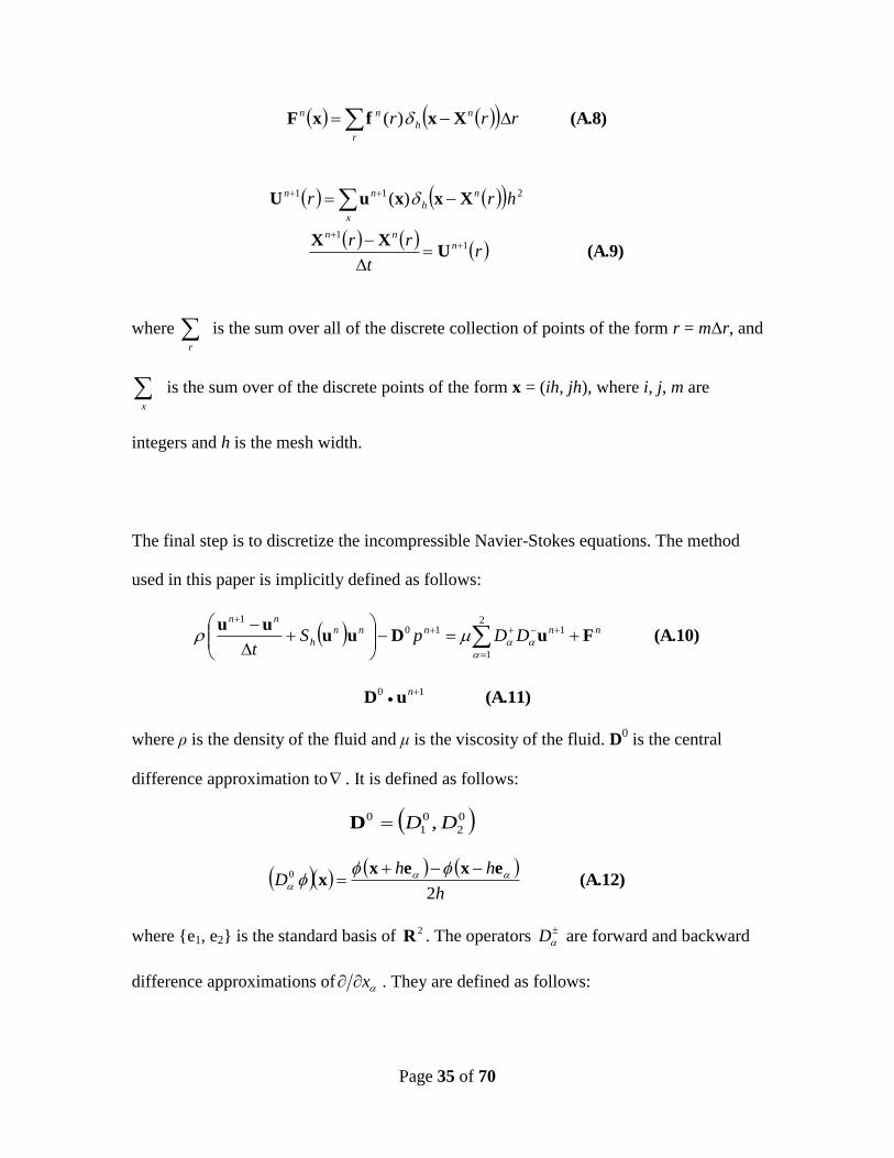
Using this choice of δh, Eqns. 5 – 6 can be discretized as follows:
Page 35 of 70
(A.8)XxfxF )( r
n
h
nn rrr
(A.9)U
XX
XxxuU
)(
11
211
rt
rr
hrr
nnn
x
n
h
nn
where r
is the sum over all of the discrete collection of points of the form r = mΔr, and
x
is the sum over of the discrete points of the form x = (ih, jh), where i, j, m are
integers and h is the mesh width.
The final step is to discretize the incompressible Navier-Stokes equations. The method
used in this paper is implicitly defined as follows:
(A.10) FuDuuuu
12
1
101
nnnnn
h
nn
DDpSt
(A.11) uD 10
n
where ρ is the density of the fluid and μ is the viscosity of the fluid. D0 is the central
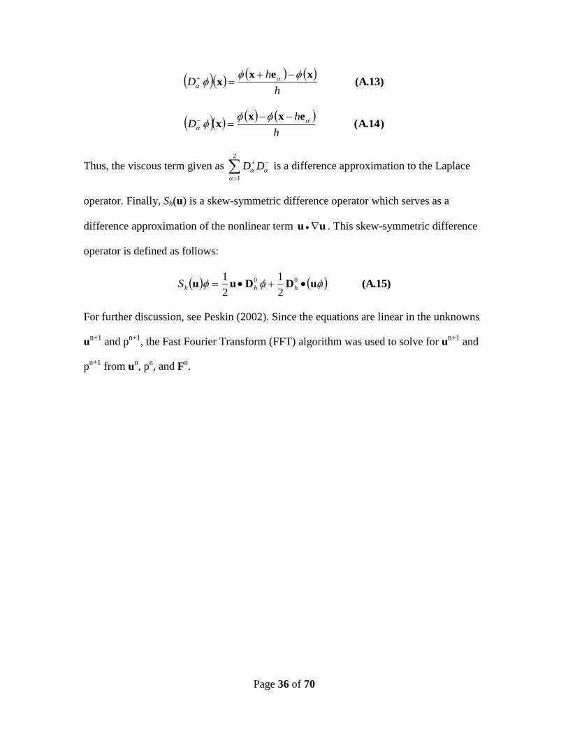
difference approximation to . It is defined as follows:
D , 0
2
0
1
0 DD
(A.12) exex
x 2
0
h
hhD
where {e1, e2} is the standard basis of 2R . The operators
D are forward and backward
difference approximations of x . They are defined as follows:
Page 36 of 70
(A.13) xex
x h
hD
)A.14( exx
x h
hD
Thus, the viscous term given as
DD2
1
is a difference approximation to the Laplace
operator. Finally, Sh(u) is a skew-symmetric difference operator which serves as a
difference approximation of the nonlinear term uu . This skew-symmetric difference
operator is defined as follows:
(A.15)uDDuu 2
1
2
1 00 hhhS
For further discussion, see Peskin (2002). Since the equations are linear in the unknowns
un+1
and pn+1
, the Fast Fourier Transform (FFT) algorithm was used to solve for un+1
and
pn+1
from un, p
n, and F
n.
Page 37 of 70
References
ALBEN, S. (2008). Optimal flexibility of a flapping appendage in an inviscid fluid. J.
Fluid Mech. 614, 355-380.
ALBEN, S. (2009). Simulating the dynamics of flexible bodies and vortex sheets. J.
Comp. Phys. 228, 2587-2603.
ALBEN, S., SHELLEY, M., AND ZHANG, J. (2002). Drag reduction through self-
similar bending of a flexible body. Nature. 420, 479-481.
ALBEN, S., SHELLEY, M., AND ZHANG, J. (2004). How flexibility induces
streamlining in a two-dimensional flow. Physics of Fluids 16(5): 1694-1713.
BENNETT, L. (1977) Clap and fling aerodynamics – an experimental evaluation. J. Exp.
Biol. 69, 261-272.
BERMAN, G. J. AND WANG, Z. J. (2007). Energy-minimizing kinematics in hovering
insect flight. J. Fluid Mech. 582, 153-168.
BIRCH, J. M., DICKSON, W. B., AND DICKINSON, M. H. (2004). Force production
and flow structure of the leading edge vortex on flapping wings at high and low
Reynolds numbers. J. Exp. Biol. 207, 1063-1072.
Page 38 of 70
CHANG, J. W. AND SOHN, M. H. (2006). Numerical flow visualization of first cycle
and cyclic motion of a rigid fling-clapping wing. J. Visualization 9(4), 1875-1897.
CHEER, A. Y. L. AND KOEHL, M. A. R. (1987). Paddles and rakes: Fluid flow through
bristled appendages of small organisms. J. Theor. Biol. 129, 17-39.
CLOUPEAU, M., DEVILLERS, J. F. AND DEVEZEAUX, D. (1979). Direct
measurements of instantaneous lift in desert locust: comparison with Jensen’s
experiments on detached wings. J. exp. Biol. 80, 1-15.
COMBES, S. A. AND DANIELS, T. L. (2003). Into thin air: contributions of
aerodynamic and inertial-elastic forces to wing bending in the hawkmoth
Manduca sexta. J. Exp. Biol. 206, 2999-3006.
DENNY, M. (1994). Extreme drag forces and the survival of wind-swept and water-
swept organisms. J. Exp. Biol. 194, 97-115.
DICKINSON, M. H. (1994). The effects of wing rotation on unsteady aerodynamic
performance at low Reynolds numbers. J. exp. Biol. 192, 179-206.
DICKINSON, M. H. and GÖTZ, K. G. (1993). Unsteady aerodynamic performance of
model wings at low Reynolds numbers. J. exp. Biol. 174, 174.
Page 39 of 70
DICKINSON, M. H., LEHMANN, F. -O., and SANE, S. P. (1999). Wing rotation and
the aerodynamic basis of insect flight. Science 284, 1954-1960.
DUDLEY, R. (2000). The biomechanics of insect flight: form, function, evolution.
Princeton: Princeton University Press.
ELLINGTON, C. P. (1980). Wing mechanics and take-off preparation of thrips
(Thysanoptera). J. Exp. Biol. 85, 129-136.
ELLINGTON, C. P. (1984a). The aerodynamics of hovering insect flight. III.
Kinematics. Phil. Trans. R. Soc. Lond. B 305, 41-78.
ELLINGTON, C. P. (1984b). The aerodynamics of hovering insect flight. IV.
Aerodynamic Mechanisms. Phil. Trans. R. Soc. Lond. B 305, 79-113.
ELLINGTON, C. P. (1999). The novel aerodynamics of insect flight: Applications to
micro-air vehicles. J. Exp. Biol. 202, 3439-3448.
ETNIER, S. A. AND VOGEL, S. (2000). Reorientation of daffodil (Narcissus:
Amaryllidaceae) flowers in wind: Drag reduction and torsional flexibility. Am. J.
Bot. 87(1), 29-32.
FAUCI, L. J. (1990). Interaction of oscillating filaments – A computational study. J.
Comput. Phys., 86, 294.
Page 40 of 70
FAUCI, L. J. AND FOGELSON, A. L. (1993). Truncated Newton methods and the
modeling of complex elastic structures. Comm. Pure Appl. Math., 46, 787.
FAUCI, L. J. AND PESKIN, C. S. A computational model of aquatic animal locomotion.
J. Comput. Phys. 77, 85.
GRUNBAUM, D. EYRE, D. AND FOGELSON, A. (1998). Functional geometry of
ciliated tentacular arrays in active suspension feeders. J. Exp. Biol., 201, 2575-
2589.
HAUSSLING, H. J. (1979). Boundary fitted coordinates for accurate numerical solution
of multibody flow problems. J. Comp. Phys. 30, 107 – 124.
HEATHCOTE, S., WANG, Z., AND GURSUL, I. (2007). Effect of spanwise flexibility
on flapping wing propulsion. J. Fluids Structures 24(2), 183-199.
HORRIDGE, G. A. (1956). The flight of very small insects. Nature 178, 1334-1335.
ISHIHARA, D., HORIE, T., AND DENDA, M. (2009). A two-dimensional
computational study on the fluid-structure interaction cause of wing pitch changes
in dipteran flapping flight. J. Exp. Biol. 212, 1-10.
Page 41 of 70
KIM, D.-K., KIM, H.-I., HAN, J.-H., AND KWON, K.-J. (2008). Experimental
investigation on the aerodynamic characteristics of a bio-mimetic flapping wing
with macro-fiber composites. J. Intel. Mat. Sys. and Struct. 19, 423.
KOEHL, M. A. R. (1984). How do benthic organisms withstand moving water? Am.
Zool. 24, 57-70.
KOEHL, M. A. R. (1995). Fluid flow through hair-bearing appendages: Feeding,
smelling, and swimming at low and intermediate Reynolds number. In C.P.
Ellington and T. J. Pedley [eds.], Biological Fluid Dynamics, Soc. Exp. Biol.
Symp. 49, 157-182.
LAI, M. -C. AND PESKIN (2000). An immersed boundary method with formal second
order accuracy and reduced numerical viscosity. Journal of Computational
Physics 160, 705-719.
LAUDER, G. V., MADDEN, P. G. A., MITTAL, R., DONG, H. AND BOZKURTTAS,
M. (2006). Locomotion with flexible propulsors: I. Experimental analysis of
pectoral fin swimming. Bioinspir. Biomim. 1, S25-S34.
LEHMANN, F.-O., SANE, S. P., AND DICKINSON, M. (2005). The aerodynamic
effects of wing-wing interaction in flapping insect wings. J. Exp. Biol., 208(16),
3075 - 3092.
Page 42 of 70
LEHMANN, F.-O. AND PICK, S. (2007). The aerodynamic benefit of wing–wing
interaction depends on stroke trajectory in flapping insect wings. J. Exp. Biol.
210, 1362-1377.
LIGHTHILL, M. J. (1973). On the Weis-Fogh mechanism of lift generation. J. Fluid
Mech. 60, 1-17.
MARDEN, J. H. (1987). Maximum lift production during takeoff in flying animals. J.
Exp. Biol. 130, 235-258.
MAXWORTHY, T. (1979). Experiments on the Weis-Fogh mechanism of lift generation
by insects in hovering flight. Part I. Dynamics of the ‘fling.’ J. Fluid Mech. 93,
47-63.
MCQUEEN, M. C. AND PESKIN, C. S. (1997). Shared-memory parallel vector
implementation of the immersed boundary method for the computation of blood
flow in the beating mammalian heart. The Journal of Supercomputing 11(3), 213-
236.
MC QUEEN, M. C. AND PESKIN, C. S. (2000a). A three-dimensional computer model
of the human heart for studying cardiac fluid dynamics. Computer Graphics. 34,
56.
Page 43 of 70
MCQUEEN, D. M. AND PESKIN, C. S. (2001). Heart simulation by an Immersed
Boundary Method with formal second-order accuracy and reduced numerical
viscosity. In: Mechanics for a New Millennium, Proceedings of the International
Conference on Theoretical and Applied Mechanics (ICTAM) 2000, (H. Aref and
J.W. Phillips, eds.) Kluwer Academic Publishers.
MILLER, L. A. and PESKIN, C. S. (2005). A computational fluid dynamics of `clap and
fling' in the smallest insects. J. Exp. Biol., 208(2): 195 - 212.
MITTAL, R. (2006). Locomotion with flexible propulsors: II. Computational modeling
of pectoral fin swimming in sunfish. Bioinspir. Biomim. 1, S35-S41.
NORBERG, R. A. (1972). Flight characteristics of two plume moths, Alucita
pentadactyla L. and Orneodes hexadactyla L. (Microlepidoptera). Zool. Scr. 1,
241-246.
OSBORNE, M. F. M. (1951). Aerodynamics of flapping flight with application to
insects. J. Exp. Biol. 28, 221-245.
PESKIN, C. S. (2002). The immersed boundary method. Acta Numerica, 11, 479-517.
PESKIN, C. S. (1977). Flow patterns around heart valves: A numerical method. J.
Comput. Phys. 25, 220.
Page 44 of 70
SANE, S. P. (2003). The aerodynamics of insect flight. J. Exp. Biol. 206, 4191-4208.
SANE, S. P. AND DICKINSON, M. H. (2002). The aerodynamic effects of wing rotation
and a revised quasi-steady model of flapping flight. J. exp. Biol. 205, 1087-1096.
SPEDDING, G. R. AND MAXWORTHY, T. (1986). The generation of circulation and
lift in a rigid two-dimensional fling. J. Fluid Mech. 165, 247-272.
SUN, M. AND XIN, Y. (2003). Flow around two airfoils performing fling and
subsequent translation and translation and subsequent flap. Acta Mechanica
Sinica 19, 103-117.
SUNADA, S., KAWACHI, K., WATANABE, I., AND AZUMA, A. (1993).
Fundamental Analysis of three-dimensional ‘near fling.’ J. Exp. Biol. 183, 217-
248.
SUNADA, S., TAKASHIMA, H., HATTORI, T., YASUDA, K., AND KAWACHI, K.
(2002). Fluid-dynamic characteristics of a bristled wing. J. Exp. Biol. 205, 2737-
2744.
TANAKA, S. (1995). Thrips’ flight. Part 1. In Symposia ‘95 of Exploratory Research for
Advanced Technology, Japan Science and Technology Corporation, Abstracts
(ed. K. Kawachi), pp. 27–34. Tokyo: Japan Science and Technology Corporation.
Page 45 of 70
VANELLA, M., FITZGERALD, T. PREIDIKMAN, S., BALARAS, E. AND
BALACHANDRAN, B. (2009). Influence of flexibility on the aerodynamic
performance of a hovering wing. J. Exp. Biol. 212, 95-105.
VOGEL, S. (1967). Flight in Drosophila II. Variations in stroke parameters and wing
contour. J. Exp. Biol. 46, 383-392.
VOGEL, S. (1989). Drag and reconfiguration of broad leaves in high winds. J. Exp. Bot.
40, 941-948.
WANG, Z. J. (2000). Two dimensional mechanism for insect hovering. Phys. Rev. Lett.
85(10), 2216-2219.
WANG, Z. J. (2004). The role of drag in insect hovering. J. Exp. Biol. 207, 4147-4155.
WANG, Z. J. (2005). Dissecting Insect Flight. Annu.Rev. Fluid Mech. 37, 183-210.
WEIS-FOGH, T. (1973). Quick estimates of flight fitness in hovering animals, including
novel mechanisms for lift production. J. exp. Biol. 59, 169-230.
WEIS-FOGH, T. (1975). Flapping flight and power in birds and insects, conventional and
novel mechanisms. In Swimming and Flying in Nature, vol. 2 (ed. T. Y. Wu, C. J.
Brokaw and C. Brennen), pp. 729–762. New York: Plenum Press.
Page 46 of 70
WU, J. C. (1981). Theory for aerodynamic force and moment in viscous flows. AIAA J.
19, 432-441.
ZANKER, J. M. AND GÖTZ, K. G. (1990). The wing beat of Drosophila melanogaster.
II. Dynamics. Phil. Trans. R. Soc. Lond. B 327, 19-44.
ZHANG, J. Flapping dynamics of passive and active structures in moving fluid.
Submitted to Experiments in Fluids.
ZHU, L. and PESKIN, C. S. (2002). Simulation of a flapping flexible filament in a
flowing soap film by the immersed boundary method. J. Comp. Phys. 179, 452-
468.
Page 47 of 70
Figure 1: Snap shots of flight taken from high speed videos of the tiny parasitoid wasps Nasonia vitripennis (jewel wasp) and Muscidifurax raptor. Notice in both cases that the wings rotate and clap together at the end of the upstroke. The wings then rotate and translate apart and the beginning of the downstroke. Photos courtesy of Ty Hedrick.
Page 48 of 70
Figure 2: Cartoon diagram of the clap and fling of the tiny wasp Encarsia formosa. The wings clap together at the end of the upstroke (A), fling apart at the beginning of the downstroke (B,C), and finally translate away from each other (D). The fling creates a large, attached leading edge vortex for each wing. From Ellington (1999), after Weis-Fogh (1975).
Page 49 of 70
Figure 3: The peel mechanism of lift generation in insect flight from Ellington (1984). A) A two-dimensional diagram of the circulation around two wings performing a peel. B) A rigid model of ‘flat peel.’ β represents half of the angle between the wings, x represents the exposed portion of the wing, and u represents the velocity of the separation point.
Page 50 of 70
Figure 4: The clap mechanism of lift generation in insect flight from Ellington (1984). A) A two-dimensional diagram of the circulation around two wings performing a clap. The clap motion creates a jet of air downward. B) A two dimensional diagram of flexible clap or reverse peel. As the wings are clapped together, the point of attachment moves from the leading to the trailing edge of the wing.
Page 51 of 70
Figure 5: Design of the flexible wing. The fluid domain is represented as a Cartesian grid, and the boundary (wing) points are represented as red squares. These points interact with the fluid and move at the local fluid velocity. The green springs represent the bending and stretching stiffness of the boundary. The desired motion of the wing is prescribed by the target points along the top 1/5 of the wing, shown above as blue squares. These points do not interact with the fluid and they move according to the desired motion of the wing. They also apply a force to the actual boundary via the target springs. Since the target springs are only connected to the leading edge of the wing, this has the effect of making a wing with a stiff leading edge and flexible trailing edge.
Page 52 of 70
Figure 6: Translational and rotational velocities as functions of dimensionless time during the clap. For 0% overlap, translation ends before rotation begins. For 100% overlap, translation and rotation end simultaneously.
Page 53 of 70
Figure 7: Translational and rotational velocities as functions of dimensionless time during the fling. For 0% overlap, the wing completes its rotation before translation begins. For 100% overlap, the wing begins to rotate and translate simultaneously.

Page 54 of 70
Figure 8: Lift coefficients as functions of time for flexible and rigid clap and fling. A) Fling with rigid wings for 0%, 25%, 50%, 75%, and 100% overlap between the rotational and translational phases of the stroke. The first peak occurs during wing rotation, and the second peak occurs during translational acceleration. The largest lift forces are generated when rotation and translation begin at the beginning of the stroke (100% overlap). B) Fling with flexible wings. Larger peak lift forces are produced due to the peel mechanism (see results) and elastic storage. C) Clap with rigid wings. The first peak in the lift force occurs during translational acceleration. The second peak occurs during wing rotation as the wings are clapped together. D) Clap with flexible wings. Lift forces generated during clap flexible wings are very similar to the forces generated with rigid wings.
Page 55 of 70
Figure 9: Drag coefficients as functions of time for flexible and rigid clap and fling. A) Fling with rigid wings for 0%, 25%, 50%, 75%, and 100% overlap between the rotational and translational phases of the stroke. A very large peak in the drag force occurs during wing rotation as the wings are pulled apart. The largest drag forces are generated when rotation and translation begin at the beginning of the stroke (100% overlap). B) Fling with flexible wings. The peak drag forces produced are significantly lower in the flexible wing case. C) Clap with rigid wings. A large peak in the drag force occurs towards the end of the stroke as the wings are clapped together. D) Clap with flexible wings. Peak drag forces generated during clap with flexible wings are significantly lower than those generated by rigid wings.
Page 56 of 70
Figure 10: Average lift and drag coefficients generated during wing rotation and a translation of 2.5 chord lengths in the case of fling (top) and clap (bottom). A) Average lift coefficients during fling increase as the amount of rotational/translational overlap increases. In the case of 100% overlap, average lift forces are larger in the flexible case. In the other cases, average lift coefficients in the rigid and flexible cases are comparable. B) In all cases, the average drag forces produced by flexible wings are lower than those produced by rigid wings. C) In all cases, the average lift over drag produced is higher for flexible wings. This effect increases as the degree of rotational/translational overlap is increased. D) Average lift coefficients produced during clap are comparable for the rigid and flexible cases, and these forces increase as the degree of rotational/translational overlap increases. E) The average drag forces produced in the rigid wing cases are higher than the corresponding flexible wing cases. F) Average lift over drag is higher in the flexible wing cases.
Page 57 of 70
Figure 11: Lift and drag coefficients as a function of time for one-winged clap and fling with flexible wings. The amount of rotational/translational overlap was varied from 0% (translation starts at the end of rotation) to 100% (translation starts with rotation). The kinematics of the single wing are exactly the same as the kinematics of the left wing in the two-winged cases. A) Lift coefficients as a function of time for one-winged flexible fling. The first peak corresponds to the forces generated during rotation, and the second peak corresponds to the forces generated during translational acceleration. B) Lift coefficients generated during one-winged flexible clap. The first peak corresponds to the forces generated during translational acceleration. The dip in the lift force corresponds to the deceleration of the wing. As the wing rotates towards the end of the stroke, another peak in the lift force is observed. C) Drag coefficients generated during one-winged flexible fling. D) Drag coefficients generated during one-winged flexible clap.
Page 58 of 70
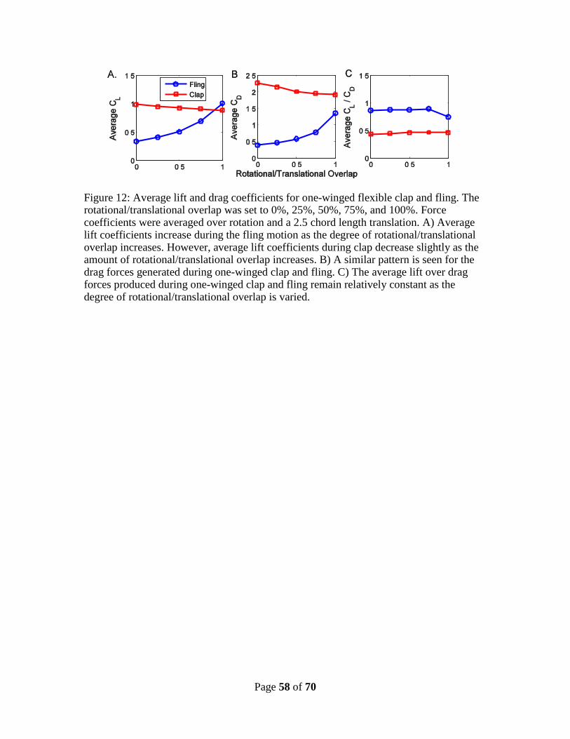
Figure 12: Average lift and drag coefficients for one-winged flexible clap and fling. The rotational/translational overlap was set to 0%, 25%, 50%, 75%, and 100%. Force coefficients were averaged over rotation and a 2.5 chord length translation. A) Average lift coefficients increase during the fling motion as the degree of rotational/translational overlap increases. However, average lift coefficients during clap decrease slightly as the amount of rotational/translational overlap increases. B) A similar pattern is seen for the drag forces generated during one-winged clap and fling. C) The average lift over drag forces produced during one-winged clap and fling remain relatively constant as the degree of rotational/translational overlap is varied.
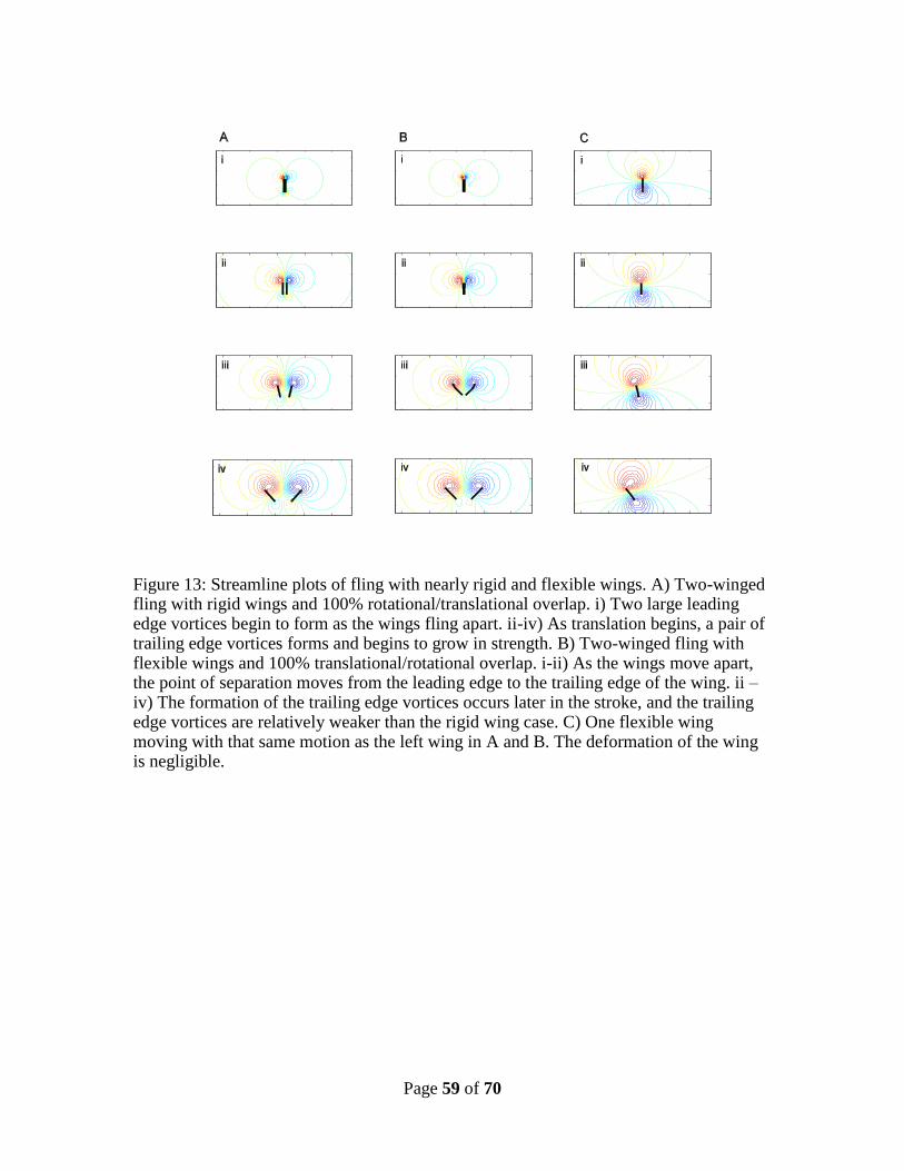
Page 59 of 70
Figure 13: Streamline plots of fling with nearly rigid and flexible wings. A) Two-winged fling with rigid wings and 100% rotational/translational overlap. i) Two large leading edge vortices begin to form as the wings fling apart. ii-iv) As translation begins, a pair of trailing edge vortices forms and begins to grow in strength. B) Two-winged fling with flexible wings and 100% translational/rotational overlap. i-ii) As the wings move apart, the point of separation moves from the leading edge to the trailing edge of the wing. ii – iv) The formation of the trailing edge vortices occurs later in the stroke, and the trailing edge vortices are relatively weaker than the rigid wing case. C) One flexible wing moving with that same motion as the left wing in A and B. The deformation of the wing is negligible.
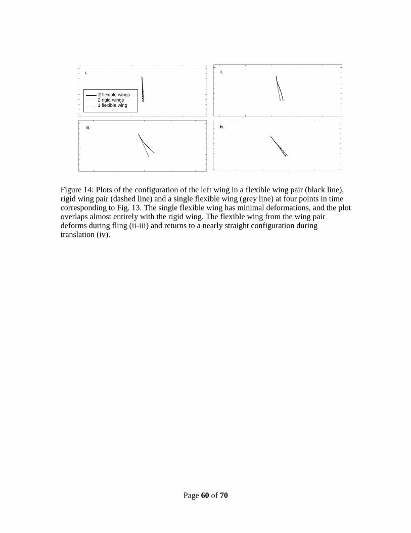
Page 60 of 70
Figure 14: Plots of the configuration of the left wing in a flexible wing pair (black line), rigid wing pair (dashed line) and a single flexible wing (grey line) at four points in time corresponding to Fig. 13. The single flexible wing has minimal deformations, and the plot overlaps almost entirely with the rigid wing. The flexible wing from the wing pair deforms during fling (ii-iii) and returns to a nearly straight configuration during translation (iv).
2 flexible wings 2 rigid wings 1 flexible wing
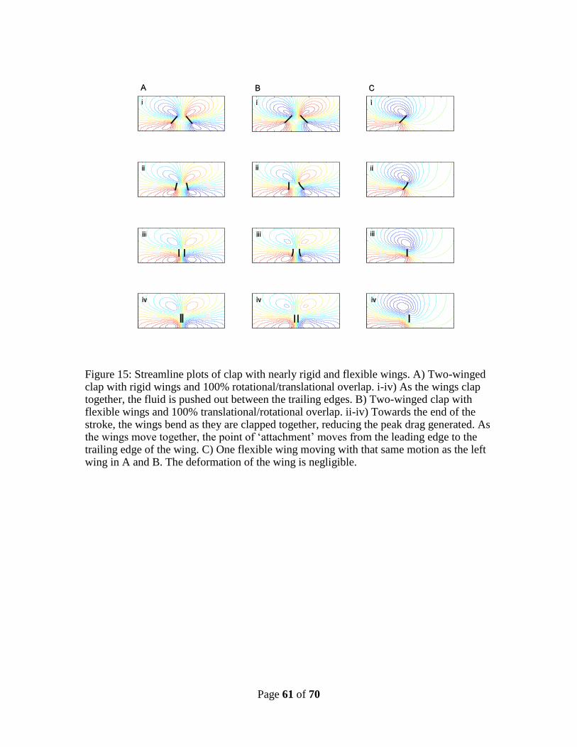
Page 61 of 70
Figure 15: Streamline plots of clap with nearly rigid and flexible wings. A) Two-winged clap with rigid wings and 100% rotational/translational overlap. i-iv) As the wings clap together, the fluid is pushed out between the trailing edges. B) Two-winged clap with flexible wings and 100% translational/rotational overlap. ii-iv) Towards the end of the stroke, the wings bend as they are clapped together, reducing the peak drag generated. As the wings move together, the point of ‘attachment’ moves from the leading edge to the trailing edge of the wing. C) One flexible wing moving with that same motion as the left wing in A and B. The deformation of the wing is negligible.
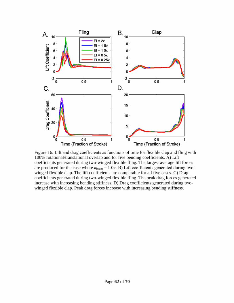
Page 62 of 70
Figure 16: Lift and drag coefficients as functions of time for flexible clap and fling with 100% rotational/translational overlap and for five bending coefficients. A) Lift coefficients generated during two-winged flexible fling. The largest average lift forces are produced for the case where kbeam = 1.0κ. B) Lift coefficients generated during two-winged flexible clap. The lift coefficients are comparable for all five cases. C) Drag coefficients generated during two-winged flexible fling. The peak drag forces generated increase with increasing bending stiffness. D) Drag coefficients generated during two-winged flexible clap. Peak drag forces increase with increasing bending stiffness.
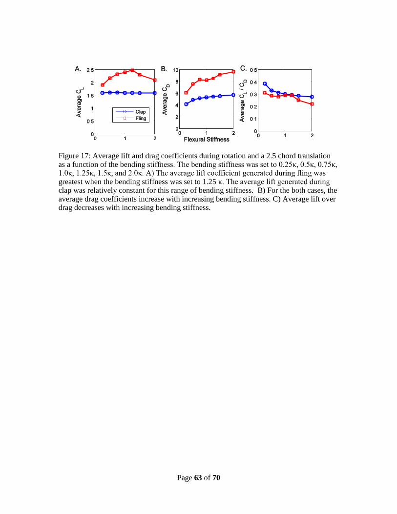
Page 63 of 70
Figure 17: Average lift and drag coefficients during rotation and a 2.5 chord translation as a function of the bending stiffness. The bending stiffness was set to 0.25κ, 0.5κ, 0.75κ, 1.0κ, 1.25κ, 1.5κ, and 2.0κ. A) The average lift coefficient generated during fling was greatest when the bending stiffness was set to 1.25 κ. The average lift generated during clap was relatively constant for this range of bending stiffness. B) For the both cases, the average drag coefficients increase with increasing bending stiffness. C) Average lift over drag decreases with increasing bending stiffness.
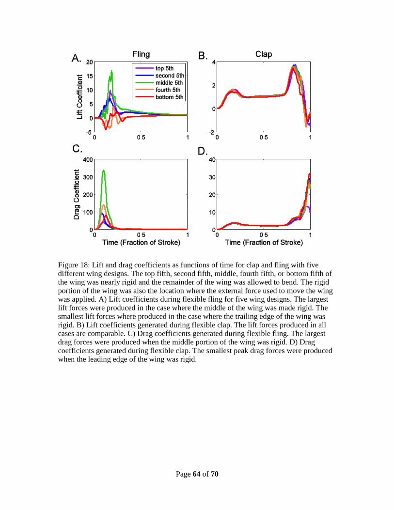
Page 64 of 70
Figure 18: Lift and drag coefficients as functions of time for clap and fling with five different wing designs. The top fifth, second fifth, middle, fourth fifth, or bottom fifth of the wing was nearly rigid and the remainder of the wing was allowed to bend. The rigid portion of the wing was also the location where the external force used to move the wing was applied. A) Lift coefficients during flexible fling for five wing designs. The largest lift forces were produced in the case where the middle of the wing was made rigid. The smallest lift forces where produced in the case where the trailing edge of the wing was rigid. B) Lift coefficients generated during flexible clap. The lift forces produced in all cases are comparable. C) Drag coefficients generated during flexible fling. The largest drag forces were produced when the middle portion of the wing was rigid. D) Drag coefficients generated during flexible clap. The smallest peak drag forces were produced when the leading edge of the wing was rigid.
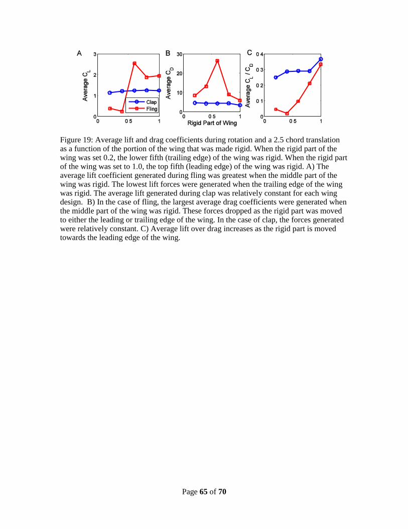
Page 65 of 70
Figure 19: Average lift and drag coefficients during rotation and a 2.5 chord translation as a function of the portion of the wing that was made rigid. When the rigid part of the wing was set 0.2, the lower fifth (trailing edge) of the wing was rigid. When the rigid part of the wing was set to 1.0, the top fifth (leading edge) of the wing was rigid. A) The average lift coefficient generated during fling was greatest when the middle part of the wing was rigid. The lowest lift forces were generated when the trailing edge of the wing was rigid. The average lift generated during clap was relatively constant for each wing design. B) In the case of fling, the largest average drag coefficients were generated when the middle part of the wing was rigid. These forces dropped as the rigid part was moved to either the leading or trailing edge of the wing. In the case of clap, the forces generated were relatively constant. C) Average lift over drag increases as the rigid part is moved towards the leading edge of the wing.
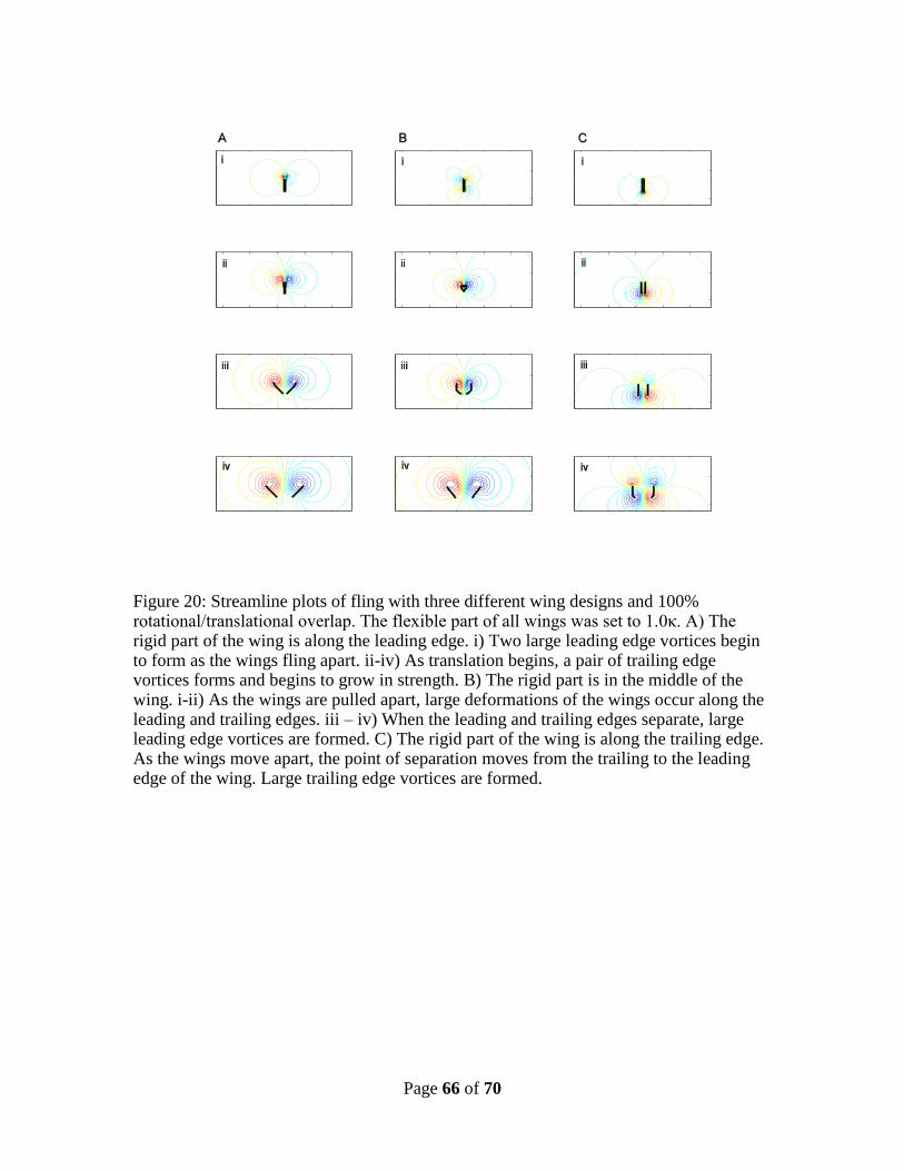
Page 66 of 70
Figure 20: Streamline plots of fling with three different wing designs and 100% rotational/translational overlap. The flexible part of all wings was set to 1.0κ. A) The rigid part of the wing is along the leading edge. i) Two large leading edge vortices begin to form as the wings fling apart. ii-iv) As translation begins, a pair of trailing edge vortices forms and begins to grow in strength. B) The rigid part is in the middle of the wing. i-ii) As the wings are pulled apart, large deformations of the wings occur along the leading and trailing edges. iii – iv) When the leading and trailing edges separate, large leading edge vortices are formed. C) The rigid part of the wing is along the trailing edge. As the wings move apart, the point of separation moves from the trailing to the leading edge of the wing. Large trailing edge vortices are formed.
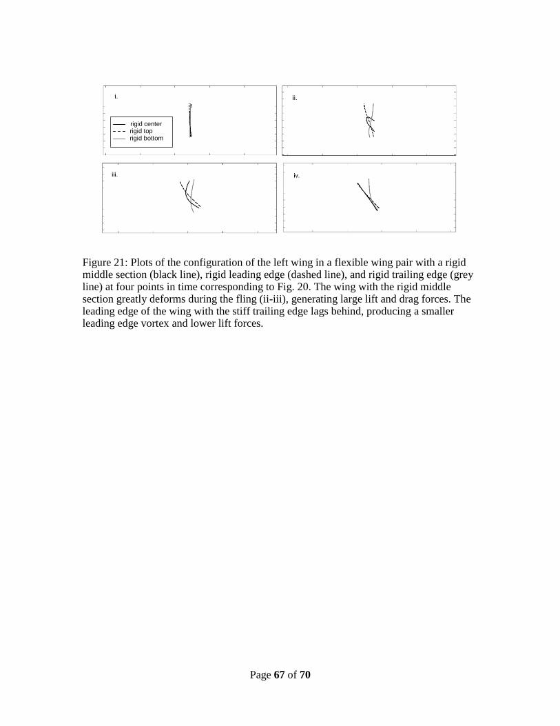
Page 67 of 70
Figure 21: Plots of the configuration of the left wing in a flexible wing pair with a rigid middle section (black line), rigid leading edge (dashed line), and rigid trailing edge (grey line) at four points in time corresponding to Fig. 20. The wing with the rigid middle section greatly deforms during the fling (ii-iii), generating large lift and drag forces. The leading edge of the wing with the stiff trailing edge lags behind, producing a smaller leading edge vortex and lower lift forces.
rigid center rigid top rigid bottom
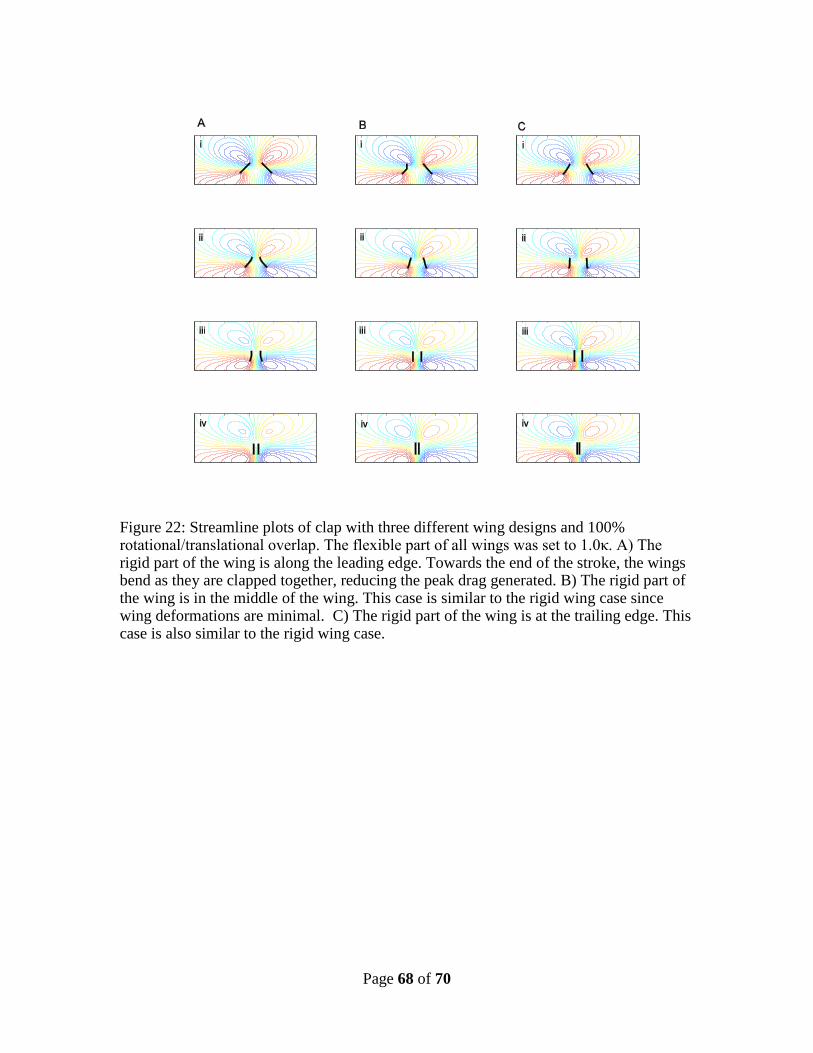
Page 68 of 70
Figure 22: Streamline plots of clap with three different wing designs and 100% rotational/translational overlap. The flexible part of all wings was set to 1.0κ. A) The rigid part of the wing is along the leading edge. Towards the end of the stroke, the wings bend as they are clapped together, reducing the peak drag generated. B) The rigid part of the wing is in the middle of the wing. This case is similar to the rigid wing case since wing deformations are minimal. C) The rigid part of the wing is at the trailing edge. This case is also similar to the rigid wing case.
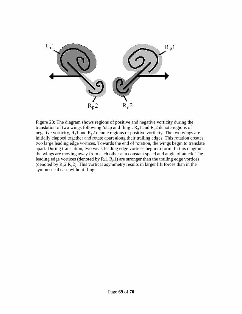
Page 69 of 70
Figure 23: The diagram shows regions of positive and negative vorticity during the translation of two wings following ‘clap and fling’. Rn1 and Rn2 denote regions of negative vorticity, Rp1 and Rp2 denote regions of positive vorticity. The two wings are initially clapped together and rotate apart along their trailing edges. This rotation creates two large leading edge vortices. Towards the end of rotation, the wings begin to translate apart. During translation, two weak leading edge vortices begin to form. In this diagram, the wings are moving away from each other at a constant speed and angle of attack. The leading edge vortices (denoted by Rn1 Rp1) are stronger than the trailing edge vortices (denoted by Rn2 Rp2). This vortical asymmetry results in larger lift forces than in the symmetrical case without fling.
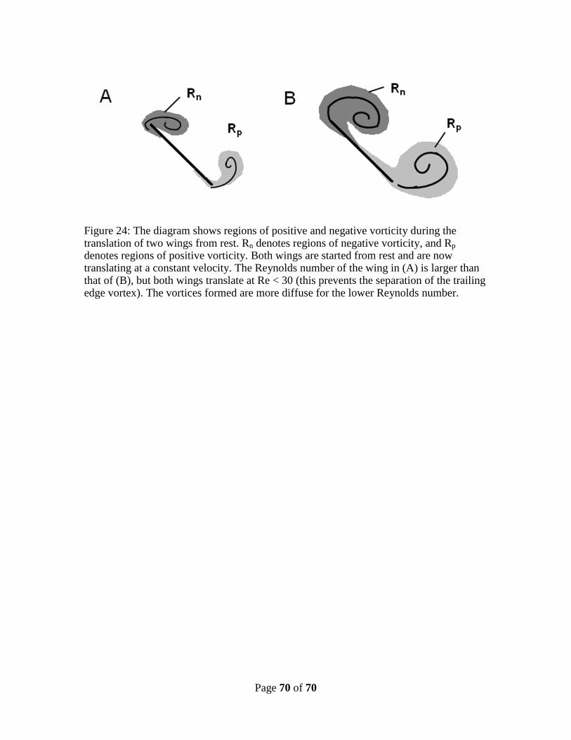
Page 70 of 70
Figure 24: The diagram shows regions of positive and negative vorticity during the translation of two wings from rest. Rn denotes regions of negative vorticity, and Rp denotes regions of positive vorticity. Both wings are started from rest and are now translating at a constant velocity. The Reynolds number of the wing in (A) is larger than that of (B), but both wings translate at Re < 30 (this prevents the separation of the trailing edge vortex). The vortices formed are more diffuse for the lower Reynolds number.