Authors:

Manuel Carmona

José María Gómez

José Bosch

Manel López

2

November/2013

Barcelona, Spain.

This work is licensed under a Creative Commons Attribution-NonCommercial-

NoDerivs 3.0 Unported License

http://creativecommons.org/licenses/by-nc-nd/3.0

3

Table of contents I. Introduction to GMSH .................................................................................................................. 4

II. Introduction to GMSH Commands ........................................................................................... 5

III. Commands for geometry generation ......................................................................................... 7

IV. Commands for meshing the geometry .................................................................................... 10

V. Examples ................................................................................................................................. 12

V.1. Example 1: Membrane ........................................................................................................ 12

V.2. Example 2: Red Blood Cell ................................................................................................. 14

VI. List of commands .................................................................................................................... 17

VII. GMSH graphics interface (GUI) ............................................................................................. 18

4

I. Introduction to GMSH

GMSH [1] is a freeware software distributed under the terms of the GNU General Public License

(GPL). It is mainly a mesh generator, provided with a CAD (Computer-Aided Design) engine and a

post-processor tool. Although having a graphical interface, one of its strong points is that it accepts

a parametric input script for the mesh generation. As an inconvenient, it is not good when trying to

define complicated geometries (for example, nowadays it is still no able to perform geometric

boolean operations, which are generally quite useful). Indeed, for complex geometries, the preferred

method is to use an external CAD software for generating the geometry and afterwards importing it

into GMSH.

As a general procedure for mesh generators (and also for GMSH), first we have to generate

geometrical entities (points, lines, areas and volumes; in this order). In GMSH there are also

physical groups, that are simply and basically a group of geometrical entities (points, lines, surfaces

or volumes). Once the geometry is defined, we have to specify (as far as possible) how the FEM

elements have to be generated. And finally, we order to mesh them (i.e., generation of the FE nodes

and elements). With GMSH we can generate some simple geometries. They are currently improving

this aspect, but at the time of this publication, only some limited geometry operations are possible.

FEM models can be generated graphically (through the GUI of GMSH), or by use of scripts (a file

containing the instructions for the mesh generation).

GMSH scripts have the extension '.geo'. In these scripts, we can define all the instructions than can

also be input graphically. The use of these scripts has many advantages:

We can re-use it for other models.

We can parameterize the model, in order to be able to change dimensions or properties

without the need to start from zero.

Portability is better. The script file occupies some kbytes, while a model can be quite large

to back it up. The only disadvantage is that it has to be re-run to get the model.

In this guide, it will be explained the language and options for creating scripts for GMSH. This

guide does not intend to substitute the GMSH guide provided with the software. It just intends to

explain the basics of GMSH scripts generation, illustrating them with examples for a better

understanding. The use of the GUI should be quite straightforward, once we know what every

option means. Moreover, the GUI interface will be better developed at lab sessions.

5

II. Introduction to GMSH Commands

First of all, we have to take into account that some of the syntax is similar to the C language (and

therefore, also to Java). This also means that, generally, commands are ended with a semicolon (';')

and that expressions are case sensitive.

Comments follow the same format than in the C language:

// for a line comment.

/* ... */ for a multiple-lines comment.

Regarding the types of variables, we can only find two different types: real and string. Their syntax

is also similar to the C language. We can highlight some keypoints:

#vector[] provides the number of elements in the vector (or list).

To ask the user for a value (and having also a default value), we can use the function

GetValue. Example:

lc = GetValue("Enter the characteristic length for the mesh: ", default_value);

We can also highlight:

The instruction Point {Point_id} provides the coordinates of a given point.

Point "*" provides the id's of all the point entities. The same for Line, Surface and Volume.

For obtaining the last number+1 associated to an entity, we can use the commands: newp

(point), newl (line), newc (curve), news (surface), newv (volumen), newll (line loop), newsl

(surface loop), newreg (any entities different than point).

Different expressions can be given separated by commas, and grouped by '{ }'.

There are some functions for strings: StrCat (concatenate two strings), Sprintf (creates a string like

'printf' would print in the C function), GetString (ask for a string to the user).

For printing in the text windows, we can use the command Printf, which have a similar format to C.

Example: Printf("Length: %g \nWidth: %g \nThickness: %g)", L,W,t);

Operators are like in C, with '^' for exponentiation. It allows the ternary operator ': ?' (reduced if).

Built-in functions are: Acos (returns a value between 0 and Pi), Asin, Atan ,Atan2, Ceil, Cos, Cosh,

Exp, Fabs, Fmod, Floor, Hypot, Log, Log10, Modulo, Rand, Sqrt, Sin, Sinh, Tan, Tanh.

We can define functions, but they are like macros, with no arguments. At the place where it is

called, it is literally substituted by the function definition. They are defined with:

Function name

Body of the function;

Return

These functions are called with the function Call: Call name;

6

':' is used to obtain a range of values with a specific increment (default to 1).

We can also build for-loops. There are two possible implementations:

For (expression : expression : expression): The last expression means the increment, and it

is optional.

For string In (expression : expression : expression): In this case, string gets the values of the

list after In.

Both for-loops finish with EndFor.

And finally, we can also build the conditional 'if': If (expression) ...... EndIf

There is no Else in GMSH.

To start a void list: string = {};

7

III. Commands for geometry generation

Geometries are generated by creating first points, then lines, afterwards surfaces and, finally

volumes. These are called elementary geometries. Each one has assigned an identifier (a number) at

the moment they are created.

Groups of elementary geometries can be formed. They are called physical entities. They have also

an identifier. Nevertheless, they cannot be modified by geometry commands.

For generating surfaces, first we have to generate what is called in GMSH 'line loops'. They are

simply a number of lines that form a closed path (and therefore, they delimitate an area).

Let's see examples of how these entities are generated.

Points:

Example: Point(1)={x,y,z,lc};

Point with id 1 is created at position x,y,z. lc is an optional parameter, indicating the size of the

elements near this point when these elements are generated.

Example for a group of points: Physical Point(5)={1,2,3,4};

Lines:

There are some different types of lines. The most basic is the straight line (Line).

Example: Line(1)={1,2};

A straight line with id 1 is created between points 1 and 2. A direction is also defined from

point 1 to point 2 in this case. This is considered the positive direction of the line.

For creating surfaces, we need to create previously a line loop.

Example: Line Loop(5)={1,2,-3,-4};

In this case a line loop with id 1 is created, and it is defined by lines with ids 1, 2, 3 and 4.

The line loop follows a direction that has to coincide with the indicated line directions. If

one line has opposite direction, a negative value for the line has to be indicated. This also

defines a direction of the surface.

Other commands for lines are: Circle, Ellipse, Spline, BSpline, Compound Line, Physical Line.

Areas (or Surfaces):

Example: Plane Surface(1)={2,3};

A plane surface with id 1 is created by using the line loops 2 and 3. The first line loop

defines the external boundaries of the surface. The rest of line loops define holes in this

area.

8

For creating volumes, we have to create surface loops. They have to define a closed volume

and with an appropriate orientation of the surfaces. Example: Surface Loop(1)={1,-2,3,-4,5,-6};

Other commands related with areas are: Ruled Surface, Compound Surface, Physical Surface.

Volumes:

Example: Volume(1)={1,2};

A volume with id 1 is created, based on surface loops 1 and 2. As in surfaces, the first

surface loop defines the external boundaries of the volume, and the rest of surface loops

define holes.

Other commands are: Compound Volume, Physical Volume.

Geometrical entities can also be generated from already existing entities. There are two of these

processes implemented in GMSH: extrusion and transformations:

Extrusion: This is a very useful method to create geometries and, at the same time, keep a "nice"

mesh.

By dragging an entity of lower level, we can generate an entity. For example, dragging a point

a certain distance in a certain direction defines a line, a line defines a surface and surface

defines a volume. This is valid not only for translations, but also for rotations. Moreover, we

can also generate at the same time the mesh of this new generated geometry.

Example: sout[]=Extrude{{tx,ty,tz},{rx,ry,rz},{px,py,pz},angle} {Line {1,2};};

The last expressions provides the entities that are going to be extruded; in this case, lines 1

and 2 (therefore, we are going to generate surfaces). {tx,ty,tz} indicates the translation

vector (direction and magnitude of translation), {rx,ry,rz} indicates the axis of rotation,

{px,py,pz} is a point in this axis of rotation and angle is the magnitude of rotation (in

radians). If we only want a translation, we only have to take the rest of parameters out of

the expression. The same reasoning is valid for only rotation.

This extrusion command returns a list (vector) of id's. The first element is the entity of the

same level than the original entity generated and the end of the extrusion. The second

element is the original entity that has been extruded. The other elements are the rest of

entities.

Transformations: There are some operations, like scaling, that can be also applied to existing

entities (or a copy of them ''Duplicata" command) for generating new ones. The operations that

we have in GMSH are:

Translate: We just need to provide the translation vector (which defines the direction and the

magnitude of translation) and the entities to be translated.

Example: Translate {-0.01, 0, 0} { Point{1}; }

9

Rotation: Like for extrusions, we have to provide a vector defining the rotation axis, a point on

the rotation axis and a rotation angle (in radians).

Example: Rotate { { 1,0,0 }, {0,0,0}, Pi/2 } {Surface {1,2,3};}

Symmetry: We just have to provide the coefficients of the equation defining the symmetry

plane ( ) and the entities to be used.

Example: Symmetry {1,0,0,0}{Duplicata{Surface{1};}};

This command generates symmetry copy of the surface 1 with respect to the YZ plane,

which passes through the point (0,0,0).

As a reminder, the coefficients A, B and C coincides with the components of a normal

vector to the plane. D can obtained with the coordinates of a point in the plane.

Dilatation: Dilatation (or compression) by homothetic transformation (like an image projection

from a light source). It requires the position of the transformation point (equivalent to the

position of the light source) and a factor (meaning how relatively far the projection is with

respect to the distance from object to the light source).

Example: Dilate { {0 ,0 ,0} , 5 }{ Duplicata { Surface {1,2}; } }

Creates an bigger version of surfaces 1 and 2, by using the point at (0,0,0) and

dilatation factor 5.

10

IV. Commands for meshing the geometry

After having defined a geometry, we should specify how the mesh has to be generated. We have

different tools for this purpose in GMSH.

First of all, GMSH has three meshing algorithms: MeshAdapt, Delaunay and Frontal. In principle

we do not have to worry on this, as GMSH uses a default algorithm depending on the geometry.

Nevertheless, we can force GMSH to use a specific algorithm. As a general rule, MeshAdapt is

good for complex surfaces, Frontal for obtaining good quality meshes and Delaunay is a fast

algorithm (also appropriate for large meshes).

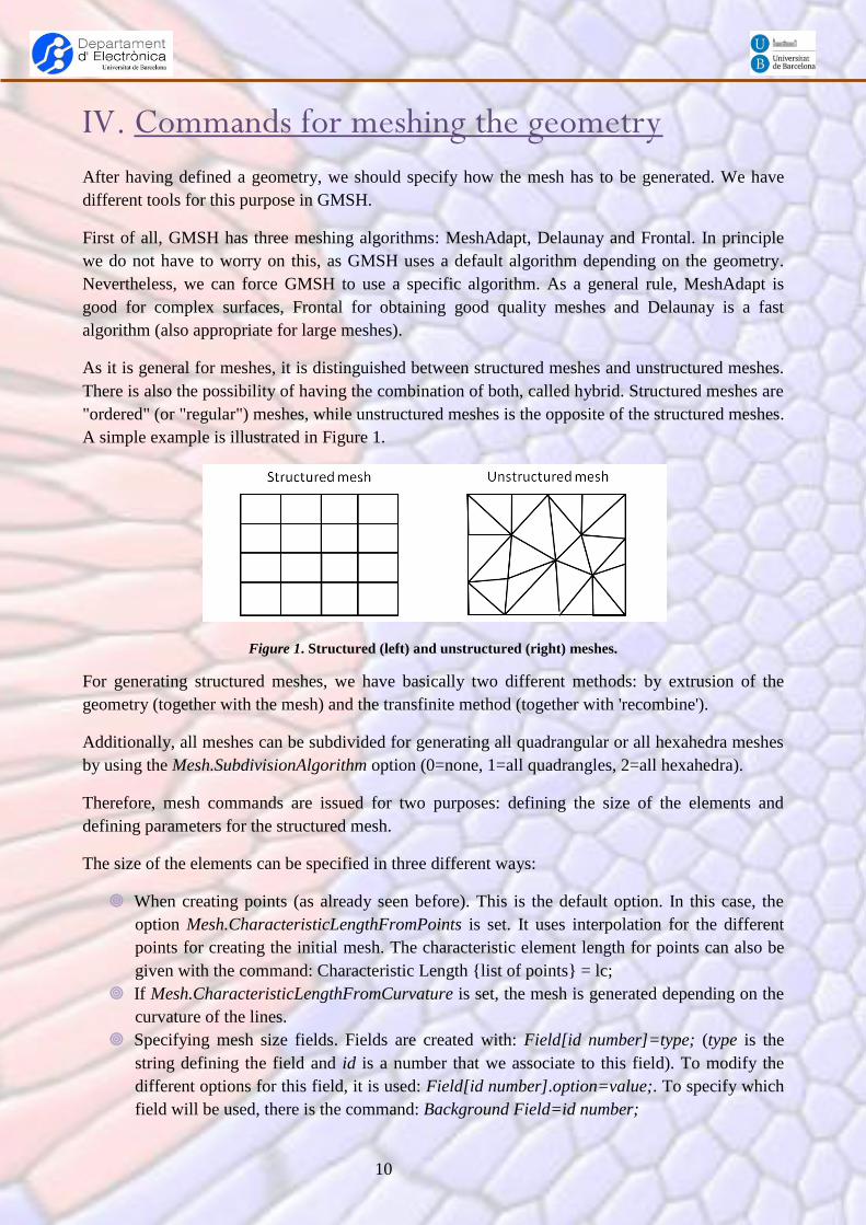
As it is general for meshes, it is distinguished between structured meshes and unstructured meshes.

There is also the possibility of having the combination of both, called hybrid. Structured meshes are

"ordered" (or "regular") meshes, while unstructured meshes is the opposite of the structured meshes.

A simple example is illustrated in Figure 1.

Figure 1. Structured (left) and unstructured (right) meshes.

For generating structured meshes, we have basically two different methods: by extrusion of the

geometry (together with the mesh) and the transfinite method (together with 'recombine').

Additionally, all meshes can be subdivided for generating all quadrangular or all hexahedra meshes

by using the Mesh.SubdivisionAlgorithm option (0=none, 1=all quadrangles, 2=all hexahedra).

Therefore, mesh commands are issued for two purposes: defining the size of the elements and

defining parameters for the structured mesh.

The size of the elements can be specified in three different ways:

When creating points (as already seen before). This is the default option. In this case, the

option Mesh.CharacteristicLengthFromPoints is set. It uses interpolation for the different

points for creating the initial mesh. The characteristic element length for points can also be

given with the command: Characteristic Length {list of points} = lc;

If Mesh.CharacteristicLengthFromCurvature is set, the mesh is generated depending on the

curvature of the lines.

Specifying mesh size fields. Fields are created with: Field[id number]=type; (type is the

string defining the field and id is a number that we associate to this field). To modify the

different options for this field, it is used: Field[id number].option=value;. To specify which

field will be used, there is the command: Background Field=id number;

11

Some of these fields are:

PostView: Specifies a background mesh, where the nodes will define the final

element sizes.

Box: Sizes in a parallelepipedic region.

Threshold: Sizes depending on the distance to an entity, which can be specified in the

Attractor field.

MathEval: Sizes depending on a mathematical function.

Min: Specifies the minimum value that can be computed with the different sizes

calculations.

Others: Max, BoundaryLayer, CenterLine, Gradient, Param, etc.

All three methods can be used at the same time. In this case, the minimum value (the most

restrictive) of them is used.

For defining structured meshes, we have:

Extrude: It works like for geometries, but additionally we have to specify, after the entities list

the command Layers or Recombine. Layers specify the number of elements to be generated

during the translation. More than one extrusions can be specified at the same time, but in this

case also a list of thicknesses for each layer has to be provided. The Recombine command

allows to generate quadrangles for 2D and prisms (or hexahedra or pyramids) in 3D.

Example: Extrude {0,0,1} {Surface{1}; Layers{ {4,1}, {0.5,0.25} }; }

Transfinite interpolation: This is used when a non-uniform distribution of element sizes are

wanted at the boundary entities. This interpolation adjust the element sizes depending on an

function depending on the coordinates.

Example for a line: Transfinite Line{1,-3}=10 Using Progression 2;

In this case, lines 1 and 3 will be meshed with 10 nodes and the nodes are distributed

spatially in a geometrical progression of 2 (following the direction of the line). We can also

use "Using Bump 2" in order to refine the mesh at both end points of the line.

It is similar for surfaces and volumes, but without the right expression for progression.

Additionally, we can also perform the following operations related to meshing:

In Surface: Embed points and lines in surfaces, so that the mesh of the surface will conform

to the mesh of the points and/or lines.

Periodical: Force the mesh of one line or surface to match the mesh on other line or surface.

Reverse Line: Change the direction of a line.

12

V. Examples

V.1. Example 1: Membrane

The first example shows one problem with many of the features that can be used in GMSH. This

example is a membrane, with different regular rectangular regions. The geo file has been generated

so that we can change the dimensions and the number of divisions without having to make again the

file. We only have to change the vectors xs and ys:

//****************

//** Parameters **

//****************

Lm=GetValue("Length of the membrane: ", 1e-3); //Membrane Length

Wm=GetValue("Width of the membrane: ", 0.5e-3); //Membrane Width

lc=Wm/15; //Default characteristic length

//Lists for the different rectangular positions on the membrane for direction x and y

xs[]={0,Lm/8,Lm/4,Lm/2,Lm};

ys[]={0,Wm/8,Wm/4,Wm/2,Wm};

nxs=#xs[]; //Number of elements in xs

nys=#ys[]; //Number of elements in ys

//**************

//** Geometry **

//**************

//Points for the membrane

p0=newp; //1

p=p0;

For indys In {0:nys-1}

For indxs In {0:nxs-1}

Point(p)={xs[indxs],ys[indys],0,lc};

p=newp; //p=p+1

EndFor

EndFor

//Horizontal lines

l0=newl; //1

l=l0;

For indys In {0:nys-1}

13

For indxs In {0:nxs-2}

Line(l)={p0+indys*nxs+indxs,p0+indys*nxs+indxs+1};

l=newl; //l=l+1

EndFor

EndFor

//Vertical lines

For indys In {0:nys-2}

For indxs In {0:nxs-1}

Line(l)={p0+indys*nxs+indxs,p0+(indys+1)*nxs+indxs};

l=newl;

EndFor

EndFor

//Line Loops

ll=newll; //1

For indys In {0:nys-2}

For indxs In {0:nxs-2}

Line Loop(ll)={l0+indxs+indys*(nxs-1),l0+(nxs-1)*nys+indys*nxs+indxs+1,-

(l0+indxs+(indys+1)*(nxs-1)),-(l0+(nxs-1)*nys+indys*nxs+indxs)};

Plane Surface(ll)={ll};

//Recombine Surface {ll};

ll=newll; //ll=ll+1

EndFor

EndFor

//**********

//** Mesh **

//**********

ss[] = Surface "*"; //All surfaces that have been generated

//Producing square elements mesh

Transfinite Surface {ss[]};

Recombine Surface {ss[]};

//Generate the volume of the membrane

Extrude {0,0,10e-6} {Surface {ss[]}; Layers {3}; Recombine;}

The resulting mesh for this case is shown in Figure 2 and Figure 3.

14

Figure 2. Mesh of the membrane.

Figure 3. Detailed view of the membrane thickness.

V.2. Example 2: Red Blood Cell

This example illustrates one possible option for generating a model of a 3D red blood cell (RBC). It

is also generated as a parametric model.

//****************

//** Parameters **

//****************

R=10e-6; // Radius of border of the RBC

Lcent=100e-6; // Length of the central part of the RBC

depr=R/4; //magnitude of the depression of central part of the RBC

th=R/5; //Thickness of the cell

lcm=R/8; //Characteristic length of the mesh

//**************

15

//** Geometry **

//**************

//First iteration for outer lines, second for inner lines

For inout In {0:1}

np=newp;

//Left circle

Point(np)={0,-R+inout*th,0,lcm};

Point(np+1)={0,0,0,lcm};

Point(np+2)={0,R-inout*th,0,lcm};

Point(np+3)={-(R-inout*th),0,0,lcm};

nl=newl;

Circle(nl)={3+(np-1),2+(np-1),4+(np-1)};

Circle(nl+1)={4+(np-1),2+(np-1),1+(np-1)};

//Top central line (with Spline)

Point(np+4)={Lcent/4,R-inout*th*0.7-depr,0,lcm};

Point(np+5)={Lcent/2,R-inout*th-depr,0,lcm};

Spline(nl+2)={3+(np-1),5+(np-1),6+(np-1)};

//Bottom central line

Point(np+6)={Lcent/4,-(R-inout*th*0.7-depr),0,lcm};

Point(np+7)={Lcent/2,-(R-inout*th-depr),0,lcm};

Spline(nl+3)={1+(np-1),7+(np-1),8+(np-1)};

EndFor

Line(nl+5)={6,np+5};

Line(nl+6)={np+7,8};

Line Loop(1)={-2,-1,3,nl+5,-(nl+2),nl,nl+1,nl+3,nl+6,-4};

Plane Surface(1)={1};

//**********

//** Mesh **

//**********

//Number of divisions on the circular lines

Transfinite Line {1,2}=Pi*R/(2*lcm);

Transfinite Line {nl,nl+1}=Pi*R/(2*lcm);

Recombine Surface {1};

//Extrussions by 90º each

ss[]=Extrude {{0,1,0},{Lcent/2,0,0},Pi/2} {Surface {1}; Layers{10}; Recombine;};

Printf("Generated first top area = %g", ss[0]);

ss1[]=Extrude {{0,1,0},{Lcent/2,0,0},Pi/2} {Surface {ss[0]}; Layers{10}; Recombine;};

Printf("Generated second top area = %g", ss1[0]);

ss2[]=Extrude {{0,1,0},{Lcent/2,0,0},Pi/2} {Surface {ss1[0]}; Layers{10}; Recombine;};

Printf("Generated third top area = %g", ss2[0]);

16

ss3[]=Extrude {{0,1,0},{Lcent/2,0,0},Pi/2} {Surface {ss2[0]}; Layers{10}; Recombine;};

Printf("Generated fourth top area = %g", ss3[0]);

The model generated by this script is shown in Figure 4 and Figure 5.

Figure 4. Mesh for the whole red blood cell.

Figure 5. Cross section view of the red blood cell.

17

VI. List of commands

Geometry: Mesh: Flux Control: Others: Point(id)={x,y,z,lc};

Line(id)={points ids};

Line Loop(id)={lines ids};

Plane Surface(id)={line loops ids};

Surface Loop(id)={surfaces ids};

Volume(id)={surface loops ids};

sout[]=Extrude{{tx,ty,tz},{rx,ry,rz},{px,py,pz},angle}

{entities; layers;};

Translate {vector} { entities}

Rotate{{vector},{point},angle}{entities};

Symmetry{A,B,C,D}{entities};

Dilate { {point coords} , factor }{ entities }

Duplicata{entities};

newp, newl, newc, news, newv, newll, newsl, newreg

Point "*"

Transfinite Line{lines ids}=#nodes;

Field[id number]=type;

Field[id number].option=value;

Function name

Body;

Return

Call name;

For (expression:expression:expression)

For var In (expression:expression:expression)

EndFor

If (expression)

EndIf

var=GetValue(string_to_show, default_value);

var=GetString(string_to_show, default_value);

Printf

Sprintf

#vec[]

//

/* */

18

VII. GMSH graphics interface (GUI)

In this chapter, we will show how the GMSH GUI works. We will use the last version of GMSH at

the moment where this publication was elaborated, i.e. version 2.8.3.

The first recommended action to perform is to indicate the name for the model that we will create.

This will define the name of the file where the commands will be saved as we are working in the

GUI creating the model. For doing this, just execute File New.

The main window of GMSH is shown in Figure 6.

Figure 6. Main window of GMSH.

The menu bar is used for opening/saving files, changing some GMSH options and setting some

graphics actions. The different submenus in this bar are shown in Figure 7.

Figure 7. Submenus in the menu bar.

We can highlight some of these options:

File Open: For opening/executing geo or msh files.

Graphics window

Menu window

Menu bar

Axis

Fast graphic commands

GMSH options

19

Tools Options: For setting all options of GMSH.

Tools Visibility: For viewing/hiding entities in the graphics window.

Tools Clipping: For viewing a cross-section of the geometry or the mesh. By holding

down left button in options A, B, C or D of the planes section and dragging the mouse, we

can change continuously the plane position or the orientation.

Tools Manipulator: For controlling precisely the orientation view in the graphics window

and the scales (zoom) in each direction independently.

At the bottom-left position there is a drop-down menu for changing some general options of

GMSH. At nearly the same position, located at the bottom bar, there is some graphics commands

for setting some view directions, rotate the view, or activating the mouse selection. The O option

allows us to set also more graphics settings (also reachable by double-left-clicking in the graphics

window). Finally, by left-clicking at the free space on this bottom bar we can view/hide the message

console.

The graphics windows is where the model and results are shown. With the mouse, we can change

continuously the orientation view: left button: rotate, right button: pan (translate), middle button:

zoom, Ctrl+left button: region zoom. All mouse and keyboard options can be obtained at the menu

bar Help KeyBoard and Mouse Usage.

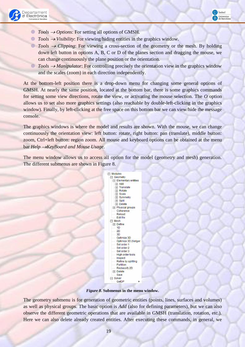
The menu window allows us to access all option for the model (geometry and mesh) generation.

The different submenus are shown in Figure 8.

Figure 8. Submenus in the menu window.

The geometry submenu is for generation of geometric entities (points, lines, surfaces and volumes)

as well as physical groups. The basic option is Add (also for defining parameters), but we can also

observe the different geometric operations that are available in GMSH (translation, rotation, etc.).

Here we can also delete already created entities. After executing these commands, in general, we

20

have the options of q for ending/aborting the addition of entities and 'e' for adding the defined

entity, but more options can appear, depending on the specific entity and operation.

The different options in this geometry menu are shown in Figure 9.

Figure 9. Options of the geometry submenu.

The mesh submenu allows to control how the mesh will be generated. The different options of this

submenu is shown in Figure 10.

Figure 10. Options of the mesh submenu.

Let's illustrate the GUI usage with one simple example. We will generate a 3D membrane, with

length lm (lm=1), width wm (wm=1) and a thickness th (th=0.2). We will define the element size

near points as lc (lc=0.1). First of all, we will define the parameters that we will use. We define

them in Geometry Elementary entities Add Parameter. We just have to click the add

button once we have defined the different fields of the parameter. The appearing windows is shown

in Figure 11, where it is illustrated the definition of the lc parameter.

21

Figure 11. Window for creating a parameter.

For creating the needed points (in our case, we only need to create four for creating also the four

boundary lines of the membrane) we can just click on the Point sheet on the same window, or just

click on Geometry Elementary entities Add Point. Points can be generated by clicking on

the graphics window where we want to place the point, or by writing the coordinates in the Point

window, that it is shown in Figure 12. Be careful not to place the mouse on the graphics windows

after you have filled the fields and before clicking the Add button because the coordinates of the

mouse will overwrite the values in the coordinate fields. If you want to do it by clicking on the

graphics window, use the Shift button to fix the coordinates in the windows even if we move the

mouse.

Figure 12. Window for creating a point.

After creating all four points (click q to end the point creation), as illustrated in Figure 13 (left), we

have to generate the lines. We have to click on Geometry Elementary entities Add Straight

line, and click on the two end points that will define the line. The line is created with a direction,

from the first point selected to the second one. We will end up with the four lines after this process,

as shown in Figure 13 (right). Click also q for finishing the creation of lines.

22

Figure 13. The four points (left) and the four lines (right) created for the membrane.

Now we will create the surface. In this case, we will create a ruled surface (i.e., a surface that can be

meshed using the transfinite interpolation). Therefore, we have to click on Geometry Elementary

entities Add Ruled Surface. In this case, we just have to click on one line, and GMSH will

find the rest (there is no other possibilities for creating a surface in our case). We have to press e to

finish the selection of lines for the surface (or q for aborting the line selection if we would have not

selected a right set of lines), and afterwards press q for definitely creating the surface. The surface

appears as shown in Figure 14. The dashed lines indicates that the surface has been created.

Figure 14. Created ruled surface of the membrane.

Before creating the volume, we will mesh the surface. In this way, when we create the volume (by

translation of this already created surface), we will also create simultaneously the volume mesh. For

this, we have to indicate two things:

We want to use transfinite interpolation for creating a regular mesh. This is done by clicking

on Mesh Define Transfinite Surface and selecting the surface (clicking on the

dashed lines). (we can select all related entities in an area by keeping pressed the Ctrl key,

while defining an area with the mouse).

We want to generate square elements and not rectangular. This is done with by clicking on

Mesh Define Recombine and selecting the same surface.

23

In order to check how the surface elements will be ,we can generate the mesh by clicking on Mesh

2D. The results should be like shown in with a mesh of 10x10 square elements. Clear them with

the bar menu option File Clear.

Figure 15. Meshed surface.

Now, let's create the volume. We will use the extrude option Geometry Elementary entities

Translate Extrude surface. We have to enter the value th value in the Z Component field.

Unfortunately, not all options are available in the GUI. For specifying the number of elements in the

extruded Z direction and indicating that we want cube-shaped elements, we will have to edit the geo

file and include Layers{3}; Recombine; inside the last field of the extrude command. The

instruction would be something like: Extrude {0, 0, th} { Surface{5}; Layers{3}; Recombine; }.

Save the file and run this file making File Open.

By generating the 3D mesh, clicking on Mesh 3D, we should obtain something similar to what is

shown in Figure 16.

Figure 16. Meshed volume.

24

Acronyms:

2D: Two-dimensional

3D: Three-dimensional

CAD: Computer Aided Design

FEM: Finite Element Method

GPL: General Public License.

RBC: Red Blood Cell

[1] http://geuz.org/gmsh/