author(s): john h. cochrane and lars peter hansen source
TRANSCRIPT

http://www.jstor.org
Asset Pricing Explorations for MacroeconomicsAuthor(s): John H. Cochrane and Lars Peter HansenSource: NBER Macroeconomics Annual, Vol. 7, (1992), pp. 115-165Published by: The University of Chicago PressStable URL: http://www.jstor.org/stable/3585001Accessed: 13/07/2008 12:16
Your use of the JSTOR archive indicates your acceptance of JSTOR's Terms and Conditions of Use, available at
http://www.jstor.org/page/info/about/policies/terms.jsp. JSTOR's Terms and Conditions of Use provides, in part, that unless
you have obtained prior permission, you may not download an entire issue of a journal or multiple copies of articles, and you
may use content in the JSTOR archive only for your personal, non-commercial use.
Please contact the publisher regarding any further use of this work. Publisher contact information may be obtained at
http://www.jstor.org/action/showPublisher?publisherCode=ucpress.
Each copy of any part of a JSTOR transmission must contain the same copyright notice that appears on the screen or printed
page of such transmission.
JSTOR is a not-for-profit organization founded in 1995 to build trusted digital archives for scholarship. We work with the
scholarly community to preserve their work and the materials they rely upon, and to build a common research platform that
promotes the discovery and use of these resources. For more information about JSTOR, please contact [email protected].

John H. Cochrane and Lars Peter Hansen UNIVERSITY OF CHICAGO, DEPARTMENT OF ECONOMICS AND NBER
Asset Pricing Explorations for Macroeconomics
1. Introduction and Overview Asset market data are often ignored in evaluating macroeconomic mod- els, and aggregate quantity data are often avoided in empirical investiga- tions of asset market returns. While there may be short-term benefits to proceeding along separate lines, we argue that security market data are among the most sensitive and, hence, attractive proving grounds for models of the aggregate economy.
An important strand of research on economic fluctuation uses models without frictions to explain the movements of aggregate quantities (e.g., Kydland and Prescott, 1982; Long and Plosser, 1983). Historically, asset market data have played little, if any, role in assessing the performance of these models. This habit is surprising. The models center on intertem-
poral decisions, and asset prices provide information about intertempo- ral marginal rates of substitution and transformation. Hence, asset market data should be valuable in assessing alternative model specifica- tions. Once the basic point that equilibrium models can explain particu- lar quantity correlations has been made, one would expect extensive use of price data in general and asset price data in particular to sort
among the many specifications of preferences and technology that give roughly similar predictions for quantity correlations.
It is sometimes argued that successful models connecting real quanti- ties to security market data may have to feature frictions, such as trans- actions costs, imperfect markets, liquidity or borrowing constraints, etc. (For an articulation of this view, see Mehra and Prescott, 1985). If, how- ever, marginal rates of substitution are disconnected from asset returns because of frictions, why should one still expect marginal rates of substi- tution to line up with marginal rates of transformation? If market fric-

116 * COCHRANE & HANSEN
tions are necessary to understand asset price data, they have potentially serious implications for the quantity predictions of business cycle models.
Perhaps the most convincing evidence for our view is that an array of researchers have studied new utility functions in an effort to address the dramatic failure of simple log or power utility models to account for basic features of asset pricing data. Although this research was not
explicitly motivated by an effort to match correlations among aggregate quantities, the proposed changes in utility functions might substantially alter important dynamic properties of the resulting models, including measures of the welfare effects of interventions or policy experiments.
Not only can security data be informative for macroeconomic model-
ing, but macroeconomic modeling should be also valuable in interpret- ing the cross-sectional and time-series behavior of asset returns. A large body of empirical work on asset pricing aims simply at reducing asset valuation to the pricing of a relatively small number of "factors," with- out explicit reference to the fundamental sources of risk. While these
dimensionality-reduction exercises can be quite useful in some contexts, it is difficult, if not impossible, to evaluate the significance of apparent asset-pricing anomalies without specifying an underlying valuation model that ties asset prices to fundamental features of the underlying economic environment, that is, without using some dynamic economic model. For example, the predictability of returns is only an anomaly given evidence that this predictability is at odds with the times series behavior of marginal rates of substitution or transformation. Clearly, documentation that expected returns on some assets vary over time "because" the expected return on the market or some factor portfolio varies over time fails to address this central issue.
As emphasized by Hansen and Richard (1987), stochastic discount fac- tors provide a convenient vehicle for summarizing the implications of
dynamic economic models for security market pricing. Alternative mod- els can imply differing stochastic discount factors. A primary aim of this
paper is to characterize the properties of the discount factors that are consistent with the behavior of asset market payoffs and prices. Such characterizations are useful for a variety of reasons. First, they provide a common set of diagnostics for a rich class of models, including new models that might be developed in the future. Second, they allow one to assess readily the information content of new financial data sets without recomputing a test of each candidate valuation model. Finally, they provide a general way of assessing the magnitude of asset-pricing puz- zles. As emphasized by Fama (1970, 1991), almost all of the empirical work in finance devoted to the documentation of apparently anomalous
Asset Pricing Explorations for Macroeconomics 117
behavior of security market payoffs and prices proceeds, implicitly or
explicitly, within the context of particular asset pricing models. Charac- terizations of stochastic discount factors that are consistent with poten- tially anomalous security market data provide a more flexible way of
understanding and interpreting the empirical findings. The remainder of this paper is organized as follows. We survey Han-
sen and Jagannathan's (1991) methods for finding feasible regions for means and standard deviations of stochastic discount factors. We then extend these characterizations by exploring additional features of dis- count factors implied by security market data. For instance, uncondi- tional volatility in discount factors can be attributed to either average conditional volatility or to variability in conditional means. We provide a characterization of this tradeoff as implied by security market data. We also quantify the sense in which candidate discount factors (implied by specific models) must be more volatile when they are less correlated with security market returns. We then apply these characterizations to reexamine a variety of stochastic discount factor models that have been
proposed in the literature. Taken together, these exercises constitute Sections 2 and 3 of our paper.
In Section 4 we follow He and Modest (1991) and Luttmer (1991) and
investigate the effects of market frictions on the implications of asset market data for analogs to stochastic discount factors. He and Modest (1991) and Luttmer (1991) have considered a variety of frictions such as short-sale constraints, bid/ask spreads or transactions costs, and bor-
rowing constraints. Not surprisingly, these market imperfections tend to loosen the link between asset returns and marginal rates of substitu- tion and transformation. However, they do not eliminate this link, and asset returns still provide useful information for dynamic economic models. We focus exclusively on borrowing constraints because of the attention these imperfections have received in the macroeconomics liter- ature and because of their potential importance in welfare analyses.
2. Interpreting Asset Market Data using the Frictionless Market Paradigm To assess the implications of asset market data for economic models and to discuss asset pricing anomalies, one needs some conceptual framework or paradigm. The frictionless market paradigm is by far the most commonly used framework, because it provides a conceptually simple and convenient benchmark. Of course, it is easy to be critical of frictionless markets. Several remarks come to mind under the heading, "the real world is complicated." Obviously, asset markets do not func-
118 * COCHRANE & HANSEN
tion exactly as described by this paradigm. At some level of inspection, market frictions such as transaction costs, short sale, and borrowing constraints must be important. Later in this essay, we will have more to say about market frictions. But a better understanding of the implica- tions of asset market data viewed through the frictionless markets para- digm is a valuable (and perhaps necessary) precursor to assessing the importance of financial market imperfections.
2.1 STOCHASTIC DISCOUNT FACTORS
Many frictionless-market empirical analyses are conducted with the ad- ditional straitjacket of tightly specified models, featuring consumers that aggregate to known, simple utility functions. Among other things, ag- gregation typically requires that consumers engage in a substantial de- gree of risk pooling. Decisive empirical evidence obtained within this straitjacket is easily misconstrued as evidence against the frictionless- market paradigm itself. The points of this subsection are: (1) to empha- size that, as long as there are no arbitrage opportunities, we can always interpret asset market data through the frictionless-market paradigm; and (2) to show that the observable implications of frictionless-market asset pricing models can be conveniently understood by characterizing the stochastic discount factors through which such models generate asset price predictions.
We begin by developing the frictionless-markets paradigm in a now and then economy.' Trading in securities markets takes place in the now time period, and payoffs to holding these securities are received in a subsequent then time period. A payoff to a security is a random variable or equivalently a bundle of contingent claims in the then time period. Consumers/investors in this economy can form portfolios of securities, without transactions costs, short sale constraints, or other impediments to trade.
The Principle of No-Arbitrage follows when consumers are not satiated in the then time period. Because consumers always want more of the numeraire good, any portfolio with a payoff that is always nonnegative and sometimes positive must have a positive price. Equivalently, any claim contingent on an event that might occur must have a positive price.
The Principle of No-Arbitrage implies that alternative ways of con- structing the same payoff must have the same cost or price, as long as there is a nontrivial, nonnegative portfolio payoff. Thus, the Principle
1. Our formulation closely follows the formulations of Ross (1976), Harrison and Kreps (1979), Kreps (1981), Hansen and Richard (1987), and Clark (1990).
Asset Pricing Explorations for Macroeconomics ? 119
of No-Arbitrage implies that each portfolio payoff must have a unique price, that is, we obtain the Law of One Price.
Consumers/investors can purchase a claim to a linear combination of
any two security market payoffs by simply purchasing the correspond- ing linear combination of the securities. The unique assignment of prices to portfolio payoffs must inherit this linearity. Thus, we can think of asset pricing in arbitrage-free frictionless-markets as a linear pricing func- tional that maps the space of asset payoffs (then) into prices (now) on the real line.
How can we think about testing the frictionless-market paradigm? We could look for two portfolios with the same payoffs, but different prices (i.e., we could test the Law of One Price), or we could look for a portfolio with a nonnegative and nontrivial payoff with a nonpositive price (i.e., test the Principle of No-Arbitrage). The detection of pure arbitrage oppor- tunities is seldom the aim of empirical work on asset prices, and conse-
quently empirical researchers typically look at security market data sets that do not imply direct violations of the Principle of No-Arbitrage. For such data sets, we can always use the frictionless markets paradigm as an interpretive device. Equivalently, we will be able to find a stochastic discount factor that will correctly price all of the observed portfolio payoffs.
As an example, suppose we use data on n primitive payoffs in an econometric analysis. For example, we may use data on the measured
one-period returns on n assets. Stack these payoffs into an n-dimen- sional random vector x with a finite second moment. A common space P of payoffs to use in econometric analyses of such assets consists of
constant-weighted portfolios of the primitive payoffs:
P = p: p = c x for some c E n}, (2.1)
where c is a vector of portfolio weights. Let the vector q denote the prices of the original payoff vector x. When all of the original security payoffs are converted into returns, q is a vector of ones. We can then construct a candidate price of a portfolio payoff, say c ? x, from prices of the original n payoffs via:
rr(C x) = c q. (2.2)
The Law of One Price is simply the implication that this price assign- ment depends only on the payoff c ? x itself and not necessarily on the choice of c used to construct this payoff. If E(xx') is nonsingular, there is only one portfolio weight that achieves any attainable payoff. Thus,
120 ? COCHRANE & HANSEN
the Law of One Price is trivially satisfied. Clearly, the use of formula (2.2) to assign prices to payoffs implies that the pricing functional Tr will be linear on P.
A stochastic discount factor is any random variable y that correctly repre- sents the prices of payoffs via the formula:
?r(p) = E(yp) for all p in P. (2.3)
The name is motivated by the fact that y is used to discount payoffs differently in alternative states of the world. Using the familiar covari- ance decomposition: cov(y, p) = E(yp) - E(y)E(p), equation (2.3) is equivalent to
Tr(p) = E(y)E(p) + cov(y, p). (2.4)
The first term on the right side of equation (2.4) uses E(y) to discount the mean payoff, and the second term adjusts for the riskiness of the payoff.
The Riesz Representation Theorem guarantees the existence of a sto- chastic discount factor as long as the Law of One Price is satisfied. For our example, it is easy to construct a stochastic discount factor y:
y* = x'E(xx')-lq. (2.5)
This is not the only discount factor, however. For instance, choose any random variable e for which E(ex) = 0. Then y* + e also is a stochastic discount factor. Define Q to be the family of all stochastic discount factors, that is, the family of all random variables with finite second moments that satisfy (2.3).
One theoretical device for generating a stochastic discount factor from an underlying model is to use the implied intertemporal marginal rate of substitution of consumers in the model economy. For instance, this is the device used in consumption-based or utility-based asset pricing theory. With a time-separable power utility function, the consumers' first-order conditions imply that equation (2.3) is satisfied for a "candi- date" stochastic discount factor given by the marginal rate of substitu- tion m:
u' (Cthen) m = p = P(Cthen/cnow)- (2.6)
U'(Cnow)

Asset Pricing Explorations for Macroeconomics ? 121
where u(c) = [cl' - 1]/(1 - -y) is the one-period power utility function, y - 0, and 3 > 0 is a subjective discount factor. Hence, if accurate
consumption data are available, the observable implications of this model specification are that m is in the set QJ of admissible stochastic discount factors.
Utility-based models typically generate strictly positive candidates for stochastic discount factors. For example, in equation (2.6), u'(Cnow) > 0 and u'(cthen) > 0 imply m > 0. More generally, Kreps (1981) and Clark (1990) show that under the Principle of No-Arbitrage, there will gener- ally exist a strictly positive stochastic discount factor. With this in mind, we let ` + + denote the subset of J consisting of all stochastic discount factors that are strictly positive. Any of these discount factors could be used to assign arbitrage-free prices to derivative claims formed from pay- offs in P or formed from other payoffs traded by consumers. Equiva- lently, they could be used to assign positive prices to any nontrivial
event-contingent claim in the then time period. Therefore, utility-based models often lead to a model-based way of constructing a strictly posi- tive candidate m in the set 9 + +.
The stochastic discount factor given in equation (2.5) might well be
negative with positive probability depending on the covariance struc- ture of the primitive payoffs and might not be in 09 + +. Similarly, incom- plete market models such as the familiar Capital Asset Pricing Model of Sharpe (1964), Lintner (1965), and Mossin (1968) and linear factor mod- els as suggested by Ross (1976) and Connor (1984) imply candidate stochastic discount factors that need not be strictly positive. The Capital Asset Pricing Model implies a candidate discount factor that is equal to a constant minus a scale multiple of the return on the wealth portfolio. More generally, exact linear factor pricing models imply stochastic dis- count factors that are linear combinations of the/an underlying collec- tion of "factors," but they do not restrict these linear combinations to be positive. Hence, whether `J or the smaller set 9 + is the relevant
family of stochastic discount factors depends on the economic models
being studied.
2.2 MOMENT IMPLICATIONS FOR DISCOUNT FACTORS
A large body of empirical work in asset pricing specifies and tests mod- els with candidate stochastic discount factors. Given a candidate m, a chi-square test is formed using the sample counterpart to the moment restriction:
E(mx - q) = 0. (2.7)
122 * COCHRANE & HANSEN
For models that imply a prespecified parametric family of such m's, one conducts the test by minimizing the hypothetical chi-square value and
adjusting the degrees of freedom according to the number of estimated
parameters (e.g., see Brown and Gibbons, 1985; Cochrane, 1992a; Ep- stein and Zin, 1991; Hansen, 1982; Hansen and Singleton, 1982; MacKin-
lay and Richardson, 1991). This approach has been partially successful to date. However, statisti-
cal measures of fit such as a chi-square test statistic may not provide the most useful guide to the modifications that will reduce pricing or other specification errors. At times, the parametric approach looks like a fishing expedition without a well-articulated strategy for finding the
promising fishing holes. Also, application of the minimum chi-square approach to estimation and inference sometimes focuses too much at- tention on whether a model is perfectly specified and not enough atten- tion on assessing model performance.
Hansen and Jagannathan (1991) suggested a complementary empiri- cal approach: Instead of proposing alternative parametric models and
testing them, begin first by characterizing the set (J or Q + + of stochastic discount factors consistent with asset pricing data and divorced from a
parametric specification. To review the simplest characterizations obtained by Hansen and Ja-
gannathan (1991), we study a regression of a discount factor y onto a constant and the vector x of asset payoffs observed by an econome- trician
y = a + x'b + e, (2.8)
where a is a constant term, b is a vector of slope coefficients, and e is the
regression error. The standard least-squares formula for the regression coefficients gives:
b [cov(x, x)]-lcov(x, y) (2.9)
a Ey - Ex'b.
Without direct data on the stochastic discount factor y, these regression coefficients cannot be estimated in the usual fashion. Instead, we can
exploit the fact that y must be a valid discount factor to infer them. The
pricing relation q = E(yx) implies
cov(x, y) = q - E(y)E(x). (2.10)

Asset Pricing Explorations for Macroeconomics ? 123
Substituting equation (2.10) into equation (2.9), we obtain
b = [cov(x, x)]-1 [q - E(y)E(x)]. (2.11)
Hence, asset information alone can be used to construct the regression coefficients b, given E(y).
Because the right-hand side variables of a regression are uncorrelated with residuals by construction,
var(y) = var(x'b) + var(e). (2.12)
It follows that var(x'b)1/2 gives a lower bound on the standard deviation of y. Thus, we have a lower bound on the standard deviation of all admissible stochastic discount factors y in J with the prespecified mean, Ey.
In our construction of a volatility bound, we considered the typical case in which no linear combination of the vector x of asset payoffs used in an econometric analysis is identically equal to one, i.e., there is no real risk-free interest rate. As a consequence, the price of a unit payoff is not known, and Ey cannot be inferred from the asset market data. Instead, we must calculate the lower bound on the standard deviation of y for each possible value of the mean. This computation leads to the lower envelope of the set of means and standard deviations of admissi- ble discount factors (in J), which we denote yS.
2.3 ASSET PRICING PUZZLES
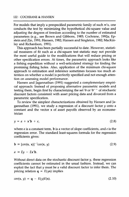
Feasible regions for mean-standard deviation pairs of stochastic dis- count factors can be used to summarize asset pricing anomalies. Figure 1 plots two such regions. The regions were constructed using quarterly data on the real value-weighted NYSE portfolio and the 3-month Trea- sury-bill returns, from 1947 to 1990. In computing the boundaries of these regions, we approximated population moments using their sam- ple counterparts. To justify this use of time series data to approximate population moments, we presume that the now-and-then economy is replicated in a stationary fashion, at least asymptotically (e.g., see Han- sen and Richard 1987).
The cup-shaped region in Figure 1 shows how much volatility in stochastic discount factors is implied by two returns often used in em- pirical analyses of the utility-based intertemporal asset pricing model. The minimum standard deviation of a discount factor y is about 0.25. Because the mean discount factor is near one, and because discount
124 * COCHRANE & HANSEN
Figure 1 BOUND ON THE STANDARD DEVIATION OF STOCHASTIC DISCOUNT FACTORS AND EQUITY PREMIUM PUZZLE
0.35 -
0.30 - 7=50
A
0.25 -
o y=40 .: A
>' 0.20 - a) -D y=30 'o A
0.15 -
0 .C.) y=20 () A
0.10 -
y=10
0.05 -
7=0 0.00 I A ,
0.85 0.90 0.95 1.00
Mean
Solid line: Minimum standard deviation of discount factors y that satisfy 1 = E(yx) for given E(y), where x = value-weighted NYSE return and Treasury Bill return. Quarterly data, 1947-1990.
Dashed line: Bound calculated from excess return, value-weighted NYSE return minus T-bill return.
Triangles: Mean and standard deviation of marginal rate of substitution generated by power utility, using quarterly nondurable and services consumption per capita,
mt+, = (Ct+l/Ct)-u -
factors have the units of inverse gross returns, this is a substantial stan- dard deviation. Figure 1 also shows us that the mean discount factor
(equal to the average of the inverse of the risk-free return if there is one) must be very near 0.998, unless we are willing to accept a dramati-
cally higher standard deviation of the discount factor. The boundary of the second region is depicted by the dashed line in
Figure 1. This boundary was computed using the excess return of stocks over bonds. Hence, it was constructed with a single security payoff with a zero price. To differentiate this region from the initial return region, we will refer to it as the Equity-Premium Region 3. In general, the bound-

Asset Pricing Explorations for Macroeconomics ? 125
ary of a feasible region for means and standard deviations constructed from a vector z of excess returns is a ray from the origin with slope [Ez'cov(z, z)-1Ez]"2 for positive values of Ey. This slope is just the "price of risk" or the asymptotic slope of the mean-standard deviation for the asset market returns used in an econometric analysis. When z is a scalar, as in our illustration, the formula for the slope collapses to the ratio of the absolute value of the mean excess return to its standard deviation. Of course, the Equity-Premium Region 2 always contains the original return region Y; however, as illustrated in Figure 1, the boundaries touch at one point.
It is not readily apparent that the region Y (or for that matter 2) is
"puzzling." Clearly, there exist stochastic discount factors that correctly price both securities on average. It only makes sense to use the term
puzzle once we have narrowed the class of asset valuation models. In other words, we cannot say that the volatility bounds for stochastic dis- count factors are excessively large without knowing how large the vola-
tility is of candidate discount factors implied by particular models. For a point of reference, and as a diagnostic for a commonly used
model, we computed sample means and standard deviations implied by representative consumer models with power utility functions. The
triangles in Figure 1 give the mean-standard deviation pair for a candi- date discount factor m constructed using formula (2.6) and aggregate quarterly per capita nondurable and services consumption data from 1947 to 1990. These calculations assume that B = 1 and the indicated range of the curvature coefficients y. Alternative choices of P can be inferred by making proportional shifts in the means and standard devia- tions.
Our statement of the Equity-Premium Puzzle is that curvature coeffi- cients y of at least 40 are required to generate the variance of discount factors implied by the equity-premium region 2 (for the triangles to lie over the dashed line). Furthermore, even if we are willing to admit curvature coefficients of 40 or more, the resulting mean-standard devia- tion pairs still do not lie in the cup because of their low means (the candidates have means Em < .85). Recall that Em is the predicted aver- age price of a unit payoff. When the riskless return is equal to this average, the riskfree rate is in excess of 17% per quarter. In effect, there is more than just an Equity-Premium Puzzle, but also a Riskfree-Rate Puzzle (see also Weil, 1989).2
2. Kocherlakota (1990) argued that increasing the subjective discount factor to values greater than one is not implausible and can be consistent with existence of equilibrium in a growing economy with infinitely lived consumers. Increasing 3 helps to "resolve" the Riskfree-Rate Puzzle but not the Equity-Premium Puzzle.

126 * COCHRANE & HANSEN
These statements of the puzzles do not involve the specific assump- tions of the Mehra and Prescott (1985) model, including a two-state Markov approximation to the distribution of consumption growth, an endowment economy, the identification of a stock index as a claim to
aggregate consumption, use of Treasury bills as a proxy for a real risk- free bond, etc. They are not specific to this particular set of assets,3 nor to postwar data. Thus, our formulation suggests that attempts to resolve the puzzle by allowing levered equity, accounting for the monetary mispricing of Treasury bills, or permitting a more general Markov struc- ture for the endowment shock are not likely to be productive.
2.4 STATISTICAL INFERENCES
In our discussion so far, we have treated sample moments as if they were equal to the underlying population moments. That is, we ab- stracted from sampling error. It is interesting to know whether the Equi- ty-Premium Puzzle and the Riskfree-Rate Puzzle still have content once we account for sampling error. To answer this question, we use statistical methods proposed by Hansen, Heaton, and Jagannathan (1992). In the
nonparametric spirit of this exercise, we use large sample central limit
approximations in making probability assessments. To test whether sampling error can account for the violation of the
volatility bounds, it is convenient to derive equivalent second moment bounds. Note that the orthogonality of the regression residual to the
right-hand side variables in the regression implies that the random vari- able a + b'x must satisfy the pricing formula (2.3) and, hence, is a stochastic discount factor in J. For a prespecified mean Ey, a + b'x also must assign a price Ey to a unit payoff. Combining these equations, we have that
E 1 [1x] a- Ey . (2.13) lX_ -b q
By premultiplying equation (2.13) by the row vector [a, b'], we obtain the following formula for the second moment of a + x'b:
E[(a + x'b)2] =[Eyq'] b (2.14)
3. Formally, one gets roughly similar bounds even if one does not use Treasury-bill data, because many other sets of assets imply about the same slope of the mean-standard deviation frontier.

Asset Pricing Explorations for Macroeconomics ? 127
This formula turns out to be quite useful for econometric inference, because it says that the second moment bound is just a linear combina- tion of the regression coefficients.
Given a candidate discount factor m, we combine relations (2.13) and (2.14) into a composite set of moment restrictions:
E{1 [ x] a
- } =0 (2.15)
E{[mq'] _m2 0.O
For instance, m might be constructed via the power utility formula (2.6). The first set of moment implications requires that a + x'b have mean Em and correctly price the payoffs q. The last moment inequality re-
quires that the candidate m satisfies the second moment bound associ- ated with Em. In contrast to the moment restrictions (2.7), the restrictions (2.15) do not require the candidate m to price assets correctly on average.
As is clear from our previous discussion, the parameters a and b can be identified and estimated using only the moment conditions in
equation (2.13). We use such estimates to approximate the asymptotic covariance matrix for the composite moment relations in (2.15) and to account for sampling variability when testing inequality (2.14).45 Be- cause of the one-sided nature of the restriction, the probability values of the resulting test statistics are one-half those of a chi-square random variable with one degree of freedom.
In Table 1 we present results for the Volatility Test just described. We
report test statistics obtained using the two original returns (value- weighted NYSE and Treasury bill) and using the single excess return. The first group of test statistics pertains to the original region YS, while
4. This strategy is very similar to one proposed by Burnside (1991) and Cecchetti, Lam, and Mark (1992).
5. From Hansen (1982) we know that the asymptotic covariance matrix can be interpreted as a spectral density matrix at frequency zero. In our empirical analysis, we followed Newey and West (1987) and used Bartlett weights to estimate this density matrix. To implement the volatility test, we transformed the sample counterparts to the moment conditions using a lower triangular decomposition of an estimate of the inverse of the asymptotic covariance matrix. The last transformed moment condition should hold with an inequality. We obtain our test statistic by minimizing the quadratic form in the transformed moment conditions by choice of a and b where the last moment condition only contributes to the sample criterion when the inequality is violated.

128 ? COCHRANE & HANSEN
Table 1 VOLATILITY TESTS USING T-BILL AND VALUE-WEIGHTED RETURNS
Returns Excess returns
y Statistic p-value Statistic p-value
1 2.19 .069 2.68 .051 5 4.93 .013 2.43 .060
10 4.90 .013 1.47 .113 15 4.76 .014 0.75 .193 20 4.61 .016 0.36 .274 30 4.30 .019 0.05 .412 40 3.99 .023 0.00 .500 50 3.66 .027 0.00 .500
The Volatility Test is a test of the moment conditions
E{[x] [1 lx [] L = and E{[m q'] [] - m2}
where m = (Cthen/C,ow)-y and x = value-weighted NYSE and T-bill returns. The asymptotic covariance matrix was estimated by weighting autocovariance j with the Bartlett weight (T- [j|)/T for Ijl < T and adding. The results reported are for T = 10.6
the second group pertains to the equity premium region 2. As is evident from Table 1, sampling error does not appear to be the explanation for the puzzles displayed in Figure 1.7 In comparing the two columns of test statistics in Table 1, recall that raising y increases volatility of the implied discount factors but has an adverse effect on the mean. The adverse mean effect is evident in test statistics based on the two returns but absent in the test statistics constructed using only the excess return.
Interestingly, the smallest probability value for the return-based tests occurs at y = 1.
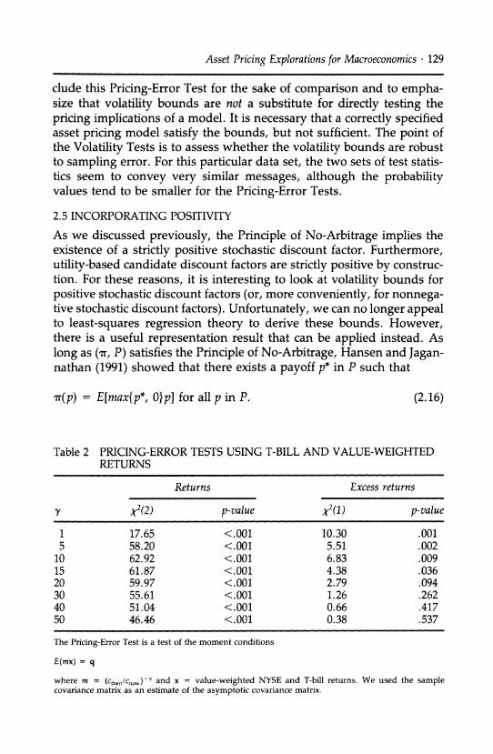
Table 2 reports a chi-square test of the pricing relation (2.7). We in-
6. The magnitude of the test statistics turned out to be sensitive to the choice of T. We also tried values of T = 5, 15, and 20. In the case of y = 1, the test statistics range from 1.63 to 2.72 when both returns were used and from 2.21 to 2.79 when the single excess return was used. In the case of y = 50, the test statistics ranged from 4.63 to 2.69 when both returns were used. Overall, the test based on both returns turned out to be more sensitive to the choice of T as might be expected because of the serial dependence in the real T-bill return.
7. When m is constant, the limiting distribution no longer applies because the only solu- tion to the moment conditions is a = m and b = 0. Hence, for m's with very low variation (values of y near zero), the performance of the volatility test statistic might be poor.
Asset Pricing Explorations for Macroeconomics . 129
clude this Pricing-Error Test for the sake of comparison and to empha- size that volatility bounds are not a substitute for directly testing the
pricing implications of a model. It is necessary that a correctly specified asset pricing model satisfy the bounds, but not sufficient. The point of the Volatility Tests is to assess whether the volatility bounds are robust to sampling error. For this particular data set, the two sets of test statis- tics seem to convey very similar messages, although the probability values tend to be smaller for the Pricing-Error Tests.
2.5 INCORPORATING POSITIVITY
As we discussed previously, the Principle of No-Arbitrage implies the existence of a strictly positive stochastic discount factor. Furthermore, utility-based candidate discount factors are strictly positive by construc- tion. For these reasons, it is interesting to look at volatility bounds for positive stochastic discount factors (or, more conveniently, for nonnega- tive stochastic discount factors). Unfortunately, we can no longer appeal to least-squares regression theory to derive these bounds. However, there is a useful representation result that can be applied instead. As
long as (rr, P) satisfies the Principle of No-Arbitrage, Hansen and Jagan- nathan (1991) showed that there exists a payoff p* in P such that
rT(p) = E[max{p*, O}p] for all p in P. (2.16)
Table 2 PRICING-ERROR TESTS USING T-BILL AND VALUE-WEIGHTED RETURNS
Returns Excess returns
X2(2) p-value X2(1) p-value
1 17.65 <.001 10.30 .001 5 58.20 <.001 5.51 .002
10 62.92 <.001 6.83 .009 15 61.87 <.001 4.38 .036 20 59.97 <.001 2.79 .094 30 55.61 <.001 1.26 .262 40 51.04 <.001 0.66 .417 50 46.46 <.001 0.38 .537
The Pricing-Error Test is a test of the moment conditions
E(mx) = q
where m = (cthen/now,)- and x = value-weighted NYSE and T-bill returns. We used the sample covariance matrix as an estimate of the asymptotic covariance matrix.

130 . COCHRANE & HANSEN
Thus, the pricing functional nT can always be represented using an op- tion on a payoff in P with a zero strike price. Clearly, max{p*, 0} is a nonnegative random variable. Hansen and Jagannathan (1991) verified that this also has the smallest second moment among nonnegative sto- chastic discount factors.
This representation leads to a characterization of the feasible region, 9y+, of mean-standard deviations for nonnegative discount factors. To apply it, we add a unit payoff to P and make up alternative prices for that payoff. Specifying a price for a unit payoff is equivalent to assigning a mean to y. This assignment is not arbitrary because the arbitrage bounds from the literature on options pricing impose limits on the range of possible prices of a unit payoff consistent with the absence of arbi- trage opportunities (see Hansen and Jagannathan, 1991, for details). For each price assignment within these bounds, we find the option on a payoff in the augmented space that satisfies the counterpart to equation (2.16). The lower envelope of 9 + is constructed by computing the stan- dard deviations of each such option.
Figure 2 gives a comparison of the boundaries of regions 9f and Y+, without and with positivity, constructed using the real value-weighted and T-bill returns as in Figure 2. Notice that the boundaries agree for ranges of Ey for which the volatility bounds are small. Once the volatil- ity bounds get larger than about 0.7, the boundaries start to depart. This pattern is easy to explain: as the standard deviation of y, whose mean is near one, rises past 0.7, the frontier y's in % are more likely to be negative in some states of the world and, hence, omitted from 9 + +. As one might therefore expect, this pattern is quite common across data sets on various assets. Hence, exploiting nonnegativity tends to be an important refinement when the original volatility bounds (for 0i) are already quite substantial.
The vertical lines in Figure 2 are used to denote the upper and lower arbitrage bounds on the mean of y. By eliminating discount factors that are negative in some states of the world, we gain considerably more information about the means of the remaining nonnegative discount factors. Where before we could only quantify a dramatic increase in the standard deviation of discount factors associated with mean discount factors far from 0.998, now we can rule out mean discount factors below about 0.98 or above 1.03. In this way, positivity makes the Riskfree-Rate Puzzle more dramatic.
Finally, for this particular data set, the corresponding excess return region S + coincides with the original excess return region 3. Conse- quently, positivity has no impact on the Equity-Premium Puzzle.

Asset Pricing Explorations for Macroeconomics ? 131
2.6 LENGTHENING THE INVESTMENT HORIZON
Next we explore the sensitivity of our findings to the "investment hori- zon" between the now and then periods. In the calculations reported so far, we used quarterly data with returns measured over the quarter. Hence, the investment horizon coincided with the sampling interval. We now expand the investment horizon to be 1 year, 2 years, and 5 years. We have (at least) three reasons for doing this. First, other empiri- cal investigations have focused on annual data to incorporate prewar data (e.g., see Grossman and Shiller, 1981; Hansen and Jagannathan, 1991; Mehra and Prescott, 1985). By including annual investment hori- zons, we will facilitate comparisons to that previous work. Second, us-
ing widely separated quarterly consumption data to measure a
long-horizon marginal rate of substitution may mitigate time-
Figure 2 VOLATILITY BOUND WITH POSITIVITY CD
i)
c 0
0
Q) -o
-c 0 -o c 0
c1r)
/ /
/ I
/
/
C4
0 1.03 0.97 0.98 0.99 1.00 1.01 1.02
Mean
Solid line: Volatility bound generated by real value-weighted NYSE and T-bill returns.
Dashed line: Bound on the standard deviation of nonnegative discount factors generated by real value- weighted NYSE and T-bill returns.
Dotted vertical lines: Arbitrage bounds on minimum and maximum mean discount factor.

132 ? COCHRANE & HANSEN
aggregation biases. Finally, to help think about solutions to asset pricing puzzles, it may be useful to assess whether these puzzles are less pro- nounced at longer horizons.
Figure 3 reports the regions for 1-, 2-, and 5-year horizons along with the previously reported quarterly horizon. The asset return data are compounded quarterly value-weighted NYSE and T-bill returns. All re- gions include the positivity restriction.
Discount factors at different investment horizons are different objects, so we expect the feasible regions for means and standard deviations to be altered as we change horizon. A two-period stochastic discount factor is a product of two consecutive one-period discount factors, so we might expect the mean of a two-period discount factor to be lower and its variance to be higher than that of a one-period discount factor. As seen in Figure 4, the bottom of the mean-standard deviation frontier shifts up and to the left as we increase the investment horizon. While the
volatility implications of the long-horizon returns are more dramatic,
Figure 3 VOLATILITY BOUNDS FOR LONG-HORIZON RETURNS o
C o
(0 1
/ -\ \ \ /
\
(D \ I
_ . \ I .
o\ Quarterly
0
_o -
- 5 Year
0o , , I
0.92 0.94 0.96 0.98 1.00 1.02 1.04
Mean
Each line gives the volatility bound on nonnegative discount factors generated by the real value- weighted NYSE and T-bill returns at the indicated horizon. Long-horizon returns are computed by
compounding quarterly returns.
o -\ / --- Quarterly
---. 2 Year
0 0.92 0.94 0.96 0.98 1.00 1.02 1.04
Mean
Each line gives the volatility bound on nonnegative discount factors generated by the real value- weighted NYSE and T-bill returns at the indicated horizon. Long-horizon returns are computed by compounding quarterly returns.

Asset Pricing Explorations for Macroeconomics . 133
there is less information about the mean of longer horizon discount factors, as reflected by the horizontal expansion of the regions.
In Figure 4 we report the two extreme boundaries (quarterly and five-year investment horizons) together with the mean-standard devia- tion pairs for the candidate discount factors constructed using power utility functions. Figure 4 extends the range of the power y beyond the values explored in Figure 1. Note that there now is a value of the power at which the quarterly candidates enter the region. However, the power is extreme, y - 210. One possible reason for entertaining large values of y follows from the work of Constantinides and Duffie (1991). They gave an illustration of a model with incomplete markets in which the
Figure 4 VOLATILITY BOUNDS AND LONG-HORIZON MARGINAL RATES OF SUBSTITUTION
Oin CA
0 O~
C3
o
._
a)
c:
'D. c 0 r> +,
4u
o
5
o 00.0 0.1 0.2 0.3 0.4 0.5 0.6 0.7 0.8 0.9 1.0 1.1 1.2
Mean
Solid lines: Volatility bounds calculated from one-quarter and 5-year real value-weighted NYSE and T-bill returns, as in Figure 3.
Lines with triangles: Mean and standard deviation of marginal rates of substitution generated by power utility,
mt+k = (Ct+k/ct)- ,
k = 1 (quarterly), k = 4 (1 year), k = 8 (2 year) and k = 20 (5 year). Symbols plotted at y increments of 10.
ul) d -
134 * COCHRANE & HANSEN
implied power for the aggregate intertemporal marginal rate of substitu- tion is a mongrel of the underlying preference parameter and the param- eters governing heterogeneity in the endowments across individuals. In their illustration, large values of y need not reflect high values of the curvature parameters in the individual preferences. (See also Mankiw, 1986, and Scheinkman, 1989, for similar observations.)
Raising consumption ratios to extremely large negative powers results in large measures of marginal rates of substitution when the consump- tion ratios are less than one. In effect, large values of y magnify the effect of "bad events" for the purposes of asset pricing (see also Rietz, 1988). The mean of the power utility candidates (triangles) starts to increase when these negative growth rate observations start to dominate the sample moments of m. Because the sample moments are dominated
by a few data points, the calculations for large values of y may reflect
very poor estimates of the population moments. For this reason, inter-
preting our large y results may be treacherous. As the investment horizon increases, the Equity-Premium and Risk-
free-Rate Puzzles do not vanish, but instead appear to be more pro- nounced. For instance, larger values of y are required to enter the feasible regions. This occurs because there are fewer and fewer con-
sumption growth observations less than one at longer horizons.8 In the extreme case of a 5-year investment horizon, the mean discount factor
always declines as y increases, and the standard deviation never ap- proaches the bounds. In this case, there are no 5-year consumption ratios that are less than one in our sample. Of course, the sample infor- mation for the longer investment horizons is likely to be quite weak.
In comparing 1-year investment horizon results to those of Hansen and Jagannathan (1991), the postwar data used in constructing Figure 5 looks more puzzling because of the absence of the depression data
points with pronounced negative consumption growth rates. These ex- tra prewar data points dramatically increase the standard deviation of the model-based candidate discount factors. The turning point for the 1-year "triangle" curve occurs at y = 15, and the 1-year discount factors enter the region at -y 30 when prewar data is included.
2.7 USING CONDITIONAL INFORMATION TO DECOMPOSE UNCONDITIONAL VARIATION
The predictability of returns is another apparent puzzle that has re- ceived a lot of attention in the finance literature (see Fama, 1991, for a review). For this reason, we follow Hansen and Richard (1987) by
8. The number of negative consumption growth rate observations in our sample is 33 for a one-quarter, 20 for a 1-year, 7 for a 2-year, and 0 for a 5-year horizon.
Asset Pricing Explorations for Macroeconomics . 135
introducing formally conditioning information into our setup. Let '6 de- note a conditioning information set available to economic agents and to econometricians in the now period, which naturally includes the prices of securities.9 Asset prices must obey
q = E(yxl|I). (2.17)
There are a variety of ways in which we can exploit conditioning information in W6. For instance, conditioning information can be used to
sharpen the unconditional volatility bounds. Alternatively, conditioning information can be used to split the unconditional variance into two
components: the average conditional variance and the variance of the conditional mean:
var(y) = E[var(yJl6)] + var[E(yj 6)]. (2.18)
If returns were unpredictable, all unconditional variance would be due to conditional variance, and none to variation in the conditional mean.
Knowledge of the split between the two components would help us to understand better the information in asset market data about condi- tional moments of the stochastic discount factors.
Asset market data turns out to contain information about how to make this split in variance. In light of relation (2.18), this split also has
implications for the unconditional variance of stochastic discount factors
implied by the conditional moments of asset returns. We describe briefly how to form feasible regions for the pair {E[var(y I6)], var[E(y l6)]}. More details are provided in Appendix 1. First, we use the fact that any y on the {E[var(yJlC)], var[E(yl1S)]} frontier must also be on the conditional (on '6) mean-standard deviation frontier for y. If not, one could lower conditional variance with no effect on conditional mean. Gallant, Han- sen, and Tauchen (1990) provided a two-(conditional) dimensional char- acterization of the latter frontier. Using their characterization, we find the frontier for {E[var(y I 6)], var[E(y l6)]} by solving a constrained mini- mization problem: choose a y on the conditional mean-standard devia- tion frontier to minimize E[var(y l')] given var[E(yl'6)].
To compute such frontiers, we need a model of the first and second conditional moments of asset returns and the candidates. Our model is formed from regressions of the log returns and log consumption ratios on the value-weighted dividend/price ratio, the lagged log T-bill return, and the term premium. For simplicity, we assume the conditional covar- iance matrix for log returns and log consumption growth is constant,
9. The analysis permits consumers to observe more information than econometricians.
136 * COCHRANE & HANSEN
and estimate it as the residual covariance matrix in the forecasting re-
gression. We then infer the first two conditional moments of the levels of consumption growth and returns assuming lognormality. (Incorpo- rating more sophisticated models of conditional heteroskedasticity or more flexible laws of motion might lead to valuable improvements on these calculations.)
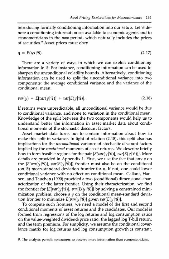
Figure 5 presents our results. Notice that most of the unconditional variance of discount factors comes from conditional variance; only a narrow range of variation in the conditional mean discount factor is consistent with the data. This makes sense, because the real return on
Treasury-bills is nearly riskless and is nearly constant over time. Also, notice that the unconditional standard deviation bound for discount
Figure 5 CONDITIONAL MOMENT BOUNDS
N c
N C4 b a_l LL
0;
u a)
0t
0
t_ c-
o c
0
E
0 0
o O
(D
c
=
0 1 2 3 4 5 6 7 8 10
Variation in conditional mean, 100xa(E(ylG)) (7. per quarter) Solid line: Bound on the root mean conditional variance versus standard deviation of conditional mean discount factor. Line with symbols: Marginal rates of substitution generated by power utility,
mt+l = (Ct+l/Ct)-'.
All calculations are based on regressions of the log value weighted return, log T-bill return and log consumption growth on the term premium, value weighted dividend/price ratio, and lagged log T-bill return.

Asset Pricing Explorations for Macroeconomics ? 137
factors is about .38, which is higher than the bound of about .24 that we encountered previously. The reason for the increase in the bound is that we have now incorporated conditioning information embedded in the conditional first and second moments of returns to sharpen the uncon- ditional volatility bounds as in Gallant, Hansen, and Tauchen (1990).
Figure 5 also includes the corresponding conditioning information
decomposition for power utility functions. For low values of the power y, the candidate discount factors have about the right predictability of conditional means, but only slight predictability is required (or allowed). However, these discount factors do not have enough conditional volatil-
ity on average. As the curvature rises, the conditional variation in- creases, but the unconditional volatility attributed to the conditional mean becomes too extreme. Thus, the models predict dramatically too much variation in the price of a unit payoff (the reciprocal of the riskfree return).
The solid square in Figure 5 gives the volatility split for the reciprocal of the value-weighted return on the NYSE. This candidate m can be
justified under an assumption of logarithmic utility where the value-
weighted return is used as a measure of the return on the wealth portfo- lio (see Rubinstein, 1976, and Epstein and Zin, 1991). This candidate also suffers from too much variation in the conditional mean and too little conditional variation (on average).
2.8 OTHER PUZZLES
Despite the widespread attention the Equity-Premium Puzzle has re- ceived, other data sets can imply much sharper restrictions on the family of feasible stochastic discount factors. Hansen and Jagannathan (1991) found dramatic bounds implied by quarterly holding-period returns on
Treasury-bills of varying maturity. Knez (1991) found a Default-Premium Puzzle, sharp bounds implied by a data set that includes corporate and
government bounds of similar maturity. In both cases, the apparent presence of near arbitrage opportunities-highly correlated returns with similar standard deviations and slightly different means-makes the bounds dramatic, especially when positivity is incorporated. Bekaert and Hodrick (1992) found sharp volatility bounds for stochastic discount factors implied by security payoffs and prices constructed from data on
foreign exchange and international equity markets. Cochrane (1992b) constructed volatility bounds implied by a linearized present value model. In addition, these techniques can elegantly address many empir- ical questions relating to traditional factor pricing models in finance. For
example, Snow (1991) recast the Small Firm Effect as set of implications for a variety of moments of stochastic discount factors.

138 * COCHRANE & HANSEN
3. Other Candidate Discount Factors The equity premium and related puzzles has given rise to an industry of "solutions." One class of "solutions" preserves the frictionless-markets framework, but modifies preferences or technology to produce the ap- propriate mean and standard deviation of discount factors. Space does not allow us a complete review of all the preferences that have been
proposed, but these may give some of the flavor.
3.1 HABIT PERSISTENCE
Constantinides (1990), Heaton (1991), and Ferson and Constantinides (1991) have looked at implications of models in which consumers' pref- erences display habit persistence. In these preference orderings, a high value of consumption yesterday raises the marginal utility of consump- tion today. For instance, the time t period utility function now depends on ct - Oct_1 instead of just ct where 0 is positive. As a result of the positive value of 0, a given series on consumption is transformed into a more volatile marginal rate of substitution series. The marginal rate of substitution for this utility function can be expressed as
m /t (Act)- (ACt+l - 0) 7 - _O(Act+l)-? Et+l (ACt+2 -- 0)-Y ?,. = PtAc,)- -
(3.1) (Act - O)-' - p0(ACt)-Y Et(ACt+1 - 0)-
(
where Act = ct/lct_ and Et is the expectation operator conditioned on time t information.
Notice that formula (3.1) requires the evaluation of some conditional expectations. To get a rough idea of how the resulting stochastic dis- count factor behaves, we made the simplifying assumption that con- sumption growth rates are independent and identically distributed over time. This allowed to us to approximate conditional expectations by their unconditional counterparts. For a more serious investigation of the properties of the implied stochastic discount factors, a reader should consult Gallant, Hansen, and Tauchen (1990) and Heaton (1991). Among other things, Heaton's analysis includes an explicit model of consumption growth at finer than quarterly frequencies and addresses the issue of time-aggregation biases.
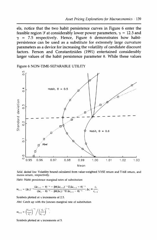
Figure 6 includes calculations of the mean and standard deviation of this candidate discount factor, using habit parameters 0 = 0.5 and 0 = 0.6. Figure 6 contains two curves indexed by the choice of 0. As Figure 6 shows, the effect of habit persistence is to raise both the mean and the standard deviation of the discount factor for a given power coefficient y. In comparing models with habit persistence to the time separable mod-
Asset Pricing Explorations for Macroeconomics * 139
els, notice that the two habit persistence curves in Figure 6 enter the feasible region Y at considerably lower power parameters, y = 12.5 and y = 7.5 respectively. Hence, Figure 6 demonstrates how habit-
persistence can be used as a substitute for extremely large curvature
parameters as a device for increasing the volatility of candidate discount factors. Ferson and Constantinides (1991) entertained considerably larger values of the habit persistence parameter 0. While these values
Figure 6 NON-TIME-SEPARABLE UTILITY
o o0
Habit. ? = 0.5
c
o
-)
k_:
0 -O C C
0
0
CN
0
0
r_'
Habit, 0 = 0.6 0,'
o.
Z' Abel
0.95 0.96 0.97 0.98 0.99 1.00 1.01 1.02 1.03
Mean
Solid, dashed line: Volatility bound calculated from value-weighted NYSE return and T-bill return, and excess return, respectively.
Habit: Habit persistence marginal rates of substitution
(Act+1 - 0)-Y - p(ACt+l)-' E(Act+2 - 0)-' c, m,,, = (AC,)-" AC, rmt+1 = (5Ct Y (Ac - 0)-Y- (0(Act)-YE(Act+l 0- ) ,ct
Symbols plotted at y increments of 2.5.
Abel: Catch up with the Joneses marginal rate of substitution
(Mt+l, C - / C_
-y
Symbols plotted at y increments of 5.
140 * COCHRANE & HANSEN
of 0 further increase the volatility of the candidate m, values of 0 close to one can lead to the consumers being "satiated" in numeraire con-
sumption good, i.e., the numerator and denominator terms of (3.1) can be negative (see Heaton, 1991, for some examples).
Abel (1990) argued for a form of habit persistence he calls "catch up with the Joneses" utility, in which the time t utility function of an indi- vidual consumer depends on the ratio ct/c_l and ct_ is aggregate con-
sumption in the previous time period. Individual consumers treat the aggregate parametrically, so they presume that their own consumption behavior cannot influence the aggregate. The idea is that you only care how well you do relative to everyone else. In the equilibrium c' = ct, this specification of preferences leads to a stochastic discount factor:
Ct+1 t1 mt+ (
/t (+ ) (3.2) ct / C\t-i/
Note that the conditional expectations that enter equation (3.1) are ab- sent from equation (3.2). The marginal rate of substitution enters the feasible region at a value of y around 40. Because Em now always in- creases with y, the difference between the equity-premium region 3 and the original return region y is less critical in assessing the model. In other words, while there still seems to be an Equity-Premium Puzzle, the Riskfree-Rate Puzzle is much less evident with this preference speci- fication.
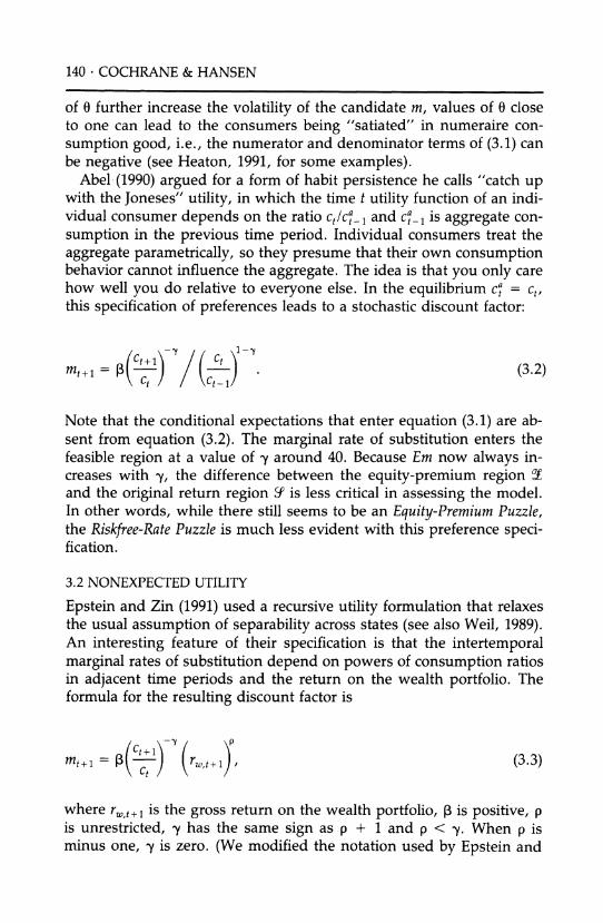
3.2 NONEXPECTED UTILITY
Epstein and Zin (1991) used a recursive utility formulation that relaxes the usual assumption of separability across states (see also Weil, 1989). An interesting feature of their specification is that the intertemporal marginal rates of substitution depend on powers of consumption ratios in adjacent time periods and the return on the wealth portfolio. The formula for the resulting discount factor is
+ =( - w,t+ (3.3)
where rw,+1 is the gross return on the wealth portfolio, P is positive, p is unrestricted, y has the same sign as p + 1 and p < y. When p is minus one, y is zero. (We modified the notation used by Epstein and
Asset Pricing Explorations for Macroeconomics ? 141
Zin so that distinct parameters are used to capture the separate contribu- tions of the consumption growth and the return on the wealth port- folio.) The reason that market-wealth return enters in equation (3.3) is that Epstein and Zin wanted an "observable" proxy for the innovation in the equilibrium utility index. They derived such a proxy by "in-
verting" the pricing formula for market-wealth return.
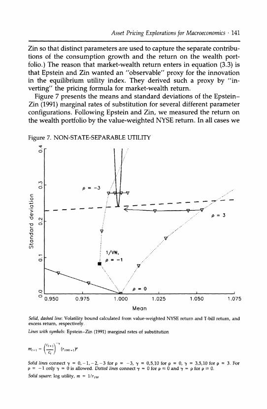
Figure 7 presents the means and standard deviations of the Epstein- Zin (1991) marginal rates of substitution for several different parameter configurations. Following Epstein and Zin, we measured the return on the wealth portfolio by the value-weighted NYSE return. In all cases we
Figure 7. NON-STATE-SEPARABLE UTILITY
0
o p = -3
C V v 7 V ,. - '
-o Cs * pc= n- o . ,
c;
1/VW,
p.,
o5 - p = -1 ..
o I I-'- .
0.950 0.975 1.000 1.025 1.050 1.075
Mean
Solid, dashed line: Volatility bound calculated from value-weighted NYSE return and T-bill return, and excess return, respectively. Lines with symbols: Epstein-Zin (1991) marginal rates of substitution
Mt+ = CJt) (rvwt+)P
Solid lines connect y = 0,-1,-2,-3 for p = -3, y = 0,5,10 for p = 0, y = 3,5,10 for p = 3. For p = -1 only y = 0 is allowed. Dotted lines connect y = 0 for p s 0 and y = p for p 2 0. Solid square: log utility, m = llrvw

142 . COCHRANE & HANSEN
set 3 = 1 as a benchmark. As before, it is easy to see how changes in 3 alter the mean-standard deviation pair. Figure 8 gives four curves
depicted by solid lines and indexed by four different values of p: p = - 3, -1, 0, and 3. Movements along each curve corresponds to changes in y. When p = -1, the curve is reduced to a single point, and the
resulting m is just the reciprocal of the return on the wealth portfolio. When p = 0, the curve becomes the power utility curve depicted in
previous figures. As is evident from this picture, variability in the candidate m is en-
hanced by increasing p1, that is, having the market enter with higher (absolute) powers. Changing y has a relatively greater impact on the mean discount factor than its standard deviation. Thus, most of the
ability of this model to generate volatile discount factors comes from the contribution of the proxy for the wealth return, rather than from the contribution of consumption.
3.3 PRODUCTION-BASED MODELS
One can also build models of stochastic discount factors by exploiting intertemporal production functions. To this end, Cochrane (1991, 1992a) and Braun (1991) showed how to construct a time series of the (mar- ginal) physical returns to investment from production data given a spec- ification of an intertemporal production function and its parameters. In a frictionless-markets setting, these investment returns should obey the same pricing relations as returns constructed from security market data. One could therefore check whether physical returns to investment are
priced compatibly with security market returns. However, our earlier comments about the flexibility of the frictionless-markets paradigm also
apply to this question of pricing compatibility. Thus, it does not seem to us to be fruitful to devise a formal "test" of pricing compatibility without narrowing the class of valuation models.
Investment returns can be used more judiciously in the context of
particular valuation models that express a stochastic discount factor as a function of investment returns. For instance, Cochrane (1991) con- structed and studied a broadly based measure of the aggregate return to investment derived from an adjustment cost model of the aggregate intertemporal production technology. Such a return might provide a more comprehensive measure of the return to the wealth portfolio than the value-weighted return on the NYSE. It could be used to replace the market return in a test of the Epstein and Zin (1991) model or in tests of the traditional linear capital asset pricing model.
Alternatively, Cochrane (1992a) constructed an exact factor pricing model using returns to residential and nonresidential fixed investments
Asset Pricing Explorations for Macroeconomics ? 143
as factors. By design factor models provide additional flexibility for satis-
fying pricing relations because of the freedom to select factor loadings. For instance, the factor loadings and technology parameters in Coch- rane's model can be chosen to exactly satisfy the sample moment condi- tions for the value-weighted NYSE and T-bill returns used in this section and, hence, to satisfy the volatility bounds. However, because of the selection of factor loadings, diagnostics focusing on only the first two moments of stochastic discount factors that we study in this section may not be particularly illuminating for assessing the performance of factor models.
3.4 CORRELATION OF DISCOUNT FACTORS WITH ASSET RETURNS
As we saw in Section 2, stochastic discount factors on the mean- standard deviation frontier (on the frontier of the region U) are linear combinations of the payoff vector x and a unit payoff. In terms of the least squares regression (2.8), they are given by a + b'x. Thus, the least volatile stochastic discount factors are perfectly correlated with a payoff of a portfolio of the assets used in an econometric analysis. In other words, the R2 obtained by regressing a frontier y onto x and a constant is one. Candidate discount factors implied by alternative economic models often produce regression R2 that are substantially less than one.
Rearranging the definition of R2, we obtain
var(y) = [var(x'b)]/R2. (3.4)
This formula can be used to construct iso-R2 contours that lie above the
boundary of S. These contours are obtained by magnifying the original standard deviation bounds by the square root of the reciprocal of the R2. If a candidate discount factor is not perfectly correlated with the asset payoff vector x, it must be more volatile than the bounds derived in Section 2.
Rather than report regression R2's for alternative candidate discount factors and trace out the corresponding iso-R2 contours, it is more conve- nient to study the volatility of the least squares projection of m onto x and a constant. It follows from the analysis in Section 2 that if a candi- date m is a valid discount factor, then so is its least-squares projection onto x and a constant. Hence, the mean and standard deviation of this projection should satisfy the original bounds derived in Section 2. Clearly the standard deviation of this projection can be low, even for highly volatile candidate discount factors, if the candidates are poorly correlated with asset returns.
Figure 8 presents results obtained by initially regressing a variety of

144 * COCHRANE & HANSEN
Figure 8. VOLATILITY BOUNDS, WITH STANDARD DEVIATION OF REGRESSIONS OF CANDIDATE DISCOUNT FACTORS ON EXCESS RETURN
Epstein-Zin, p=-3 W
Habit
Power
0.80 0.85 0.90 0.95 1,00 1.05 1.10 1.15
Mean
Dashed line: Bound calculated from value-weighted NYSE return and T-bill return, and excess return, respectively.
Lines with symbols: In each case, we run a regression
mt = a + bz, + et
where zt is the excess return, VWt - TBt. The lines with symbols report the standard deviation of fitted values. They should intersect the VW - TB bound. "Habit" reports 0 = 0.5, "Epstein-Zin" reports p = -3. Symbols are plotted at y increments of 10 for "Power" and "Abel," at y increments of 5 for "Habit," and at y increments of 1 for "Epstein and Zin."
candidate discount factors onto a constant and the excess return of stocks over bonds. Hence, the feasible region of interest is the excess return region 2. The figure reports the means and standard deviations of the fitted projections.10
As is evident from the figure, the power utility and habit persistence candidate discount factors are poorly correlated with the excess return
10. We could have regressed the candidates onto a constant and both returns. This would increase variability of the projection but shrink the feasible region. A version of Figure 8 constructed with two returns looks somewhat different than Figure 8. We present the excess return version because it was more "puzzling."
o
o
N 0 Co,
o c
0
-0 C
0 -0
a)
c
n
o
o o
o o
0.75 o 0.75

Asset Pricing Explorations for Macroeconomics * 145
and, hence, their volatility is substantially reduced by the initial regres- sion. In contrast, versions of the Epstein-Zin discount factor retain a
high degree of variability once correlation with the excess return is taken into account. This is not surprising because these discount factors are constructed using (a nonlinear function of) the value-weighted NYSE return to proxy for the return on the wealth portfolio. (We have not
attempted to account for sampling error. As before, we are not propos- ing these calculations as substitutes for formal statistical testing.)
The Epstein-Zin calculations are likely to be misleading because the
value-weighted return on the NYSE may behave quite differently than true wealth portfolio returns. For instance, the aggregate investment return constructed in Cochrane (1991) is less correlated with the excess return of stocks over bonds. Furthermore, recall that the market return enters the Epstein-Zin candidate discount factors as a proxy for the innovation in the recursive utility index valuated at the equilibrium con- sumption process. Hence, an alternative strategy to construct the im- plied stochastic discount factor is to use an estimated law of motion for consumption to infer the innovation. This approach would avoid the implicit assumption that consumption coincides with dividends, and it is also likely to result in lower correlation with the excess return."1
The inclusion of the R2 dimension to the stochastic discount factor characterization adds an extra challenge to proponents of market incom- pleteness as a source of discount rate variability. Incomplete markets
may still be frictionless. In this case, each consumer's marginal rate of substitution mi should still satisfy the asset pricing equation q = E(mix), so each consumer's marginal rate of substitution should satisfy the vola- tility bounds. Thus, incomplete market models must generate individ- ual consumption growth series that are not only highly volatile, but that are also better correlated with asset payoffs than is aggregate consump- tion growth. But a model whose main assumption is that individual incomes cannot be insured in formal security markets seems designed to generate individual consumption variability that is uncorrelated with
payoffs on traded assets.12
4. Implications for Models with Borrowing Constraints In this section we consider the implications of asset market data for models in which some consumers face borrowing constraints. Our dis-
11. This second approach could also be used to provide an information-based decomposi- tion of the unconditional volatility described in Section 2.7 applied to the Epstein-Zin (1991) model.
12. It is possible to create such models. For example, Constantinides and Duffie (1992) showed how to construct examples of incomplete market economies in which individ- ual intertemporal marginal rates of substitution are valid stochastic discount factors.

146 . COCHRANE & HANSEN
cussion illustrates how market frictions can loosen the link between asset markets and measured intertemporal marginal rates of substitution based on aggregate data. Of course, borrowing constraints are only one form of market friction that might be quantitatively important. Other frictions include incomplete markets, proportional transactions costs such as bid-ask spreads, and budget constraint kinks due to taxation. We have already commented on models with incomplete markets, and we will comment briefly on transactions costs in our concluding subsec- tion. One reason we focus on models with borrowing constraints is that, in contrast to some other forms of transactions costs, their quantitative impact is not likely to be confined to high-frequency movements in the time series data. Quite the contrary, borrowing constraints, if impor- tant, should distort the pricing links to intertemporal marginal rates of substitution at low frequencies as well.
4.1 ISSUES IN MODEL FORMULATION
It is straightforward to see how an individual's Euler equation is modified
by a borrowing constraint: The Euler equality is replaced by an Euler
inequality, reflecting the presence of nonnegative Kuhn-Tucker multi-
pliers on the constraints. More thought is required to relate asset prices to economic aggregates, because aggregate consumption sums over indi- viduals who are constrained and others who are not.
For this reason, we sketch a simple model with borrowing constraints. The setup is taken from Townsend (1980) and is a simple version of one used by Bewley (1980). There are two consumer types, A and B. Their endowments of a nonstorable good oscillate between chigh and clow. Con- sumers of type A begin with Chigh and B consumers begin with clow. There is no uncertainty and no variation in the aggregate endowment. Consumers have the same time-separable power utility function.
In the absence of impediments to communication, agents would bor- row and lend to achieve constant (Pareto optimal) consumption profiles. We suppose instead that consumers are not allowed to borrow. Town- send (1980) gave a "turnpike version" of this model to justify formally the imposition of borrowing constraints through a physical impediment to communication.
In the presence of borrowing constraints, there is no trade, and the
equilibrium interest rates are set so that the unconstrained consumers are content to consume their endowments. In other words, the price q of the riskless bond is given by
q = mu = P(Clow/high) - , (4.1)

Asset Pricing Explorations for Macroeconomics ? 147
where mu is the intertemporal marginal rate of substitution of the uncon- strained consumer. Clearly, mu is greater than the intertemporal mar-
ginal rate of substitution of the constrained consumer, that is, is greater than P(Chigh/Clow)-'
We want to know what happens when an econometrician uses aggre- gate data to measure the intertemporal marginal rate of substitution. In this simple illustration, there is no aggregate variation so that the mea- sured aggregate intertemporal marginal rate of substitution, denoted ma, is just p. Consequently, the econometrician constructs a candidate that is less than the discount factor:
mu > ma = p. (4.2)
This downward bias in ma is inherited from the distortion in the inter-
temporal marginal rate of substitution of the constrained consumers. The candidate stochastic discount factor based on aggregate data implies a lower price for a one-period bond and, hence, a higher interest rate. While this "incorrect" use of aggregate data leads to a "pricing error," the price is biased in a predictable direction.
Next we modify this setup by introducing in turn two alternative means for consumers to substitute consumption over time: valued-fiat
money and a storage technology. Consider first a version of this econ- omy with valued-fiat money. If the consumers with low endowments have money, they will exchange this money for goods as long as mu in (4.1) measured at the pretrade endowment position is greater than one. Townsend (1980) showed that in a setup with a constant (noninterven- tionist) money supply, the equilibrium consumption sequences of each
agent still oscillate and that nonnegativity constraints on money bind in alternating periods. A version of equations (4.1) and (4.2) still hold for this economy with the appropriate alterations. In particular, the
equilibrium q is one in Townsend's monetary economy because the real rate of return to holding money is zero, and clow and chigh now denote equilibrium rather than endowment consumption levels. The allocation associated with the monetary equilibrium Pareto dominates that of au-
tarky; however, because the real return to holding money is less than P-~, it is still not Pareto optimal.
A storage technology with zero depreciation leads to very similar
implications. In such an economy, the intertemporal marginal rate of transformation pins down the single-period asset return, so the real interest rate is zero. One can thus reinterpret Townsend's monetary economy as one in which the equilibrium consumption oscillates be- cause consumers' nonnegativity constraints on storage bind every other
148 ? COCHRANE & HANSEN
time period. Relations (4.1) and (4.2) continue to apply for q equal to the intertemporal marginal rate of transformation determined by the storage technology.
For reasons of empirical plausibility, we are interested in observable implications that can accommodate much more general endowment pat- terns than the ones specified by the previous illustrations. For instance, it is potentially important to accommodate stochastic endowments that grow over time and stochastic technologies for transferring consump- tion from one period to the next. (Bewley, 1980, allowed for stochastic endowments in his general setup and Deaton, 1991, incorporated en- dowment growth into a stochastic environment.) Nevertheless, the ex- ample economies we discussed illustrate the following related features that occur more generally: (1) some consumers are up against borrowing constraints in equilibrium, (2) the market discount factor for pricing assets equals the intertemporal marginal rate of substitution of uncon- strained consumers, and (3) an intertemporal marginal rate of substitu- tion measured using aggregate data is less than or equal to the market discount factor and the marginal rate of substitution of unconstrained consumers.
Feature (1) does not always emerge because consumers may save to avoid the borrowing constraint in some models. For instance, by making the storage technology in the previous example productive so that the stored good is interpreted as a capital stock, the zero interest rate impli- cation is avoided. If this technology is too productive (relative to - 1) or if the utility cost to being constrained is too severe, then the borrowing constraints may not bind in equilibrium (e.g., see Bewley, 1977; Deaton, 1991; Scheinkman and Weiss, 1986). On the other hand, Deaton (1991) emphasized that endowment growth may make borrowing constraints more likely to bind in equilibrium.
Feature (2) has led some empirical researchers to attempt to identify a sample of "unconstrained" consumers (e.g., see Hayashi, 1987; Man- kiw and Zeldes, 1991; Runkle, 1991; Zeldes, 1989) and examine asset pricing implications for these individuals. In line with the calculations reported in the previous sections, we are primarily interested in asset pricing implications for aggregate time series data on consumption. Fur- thermore, as is manifested in implication (3), the measured marginal rates of substitution using aggregate data should still be informative even though they are "contaminated" by the consumption of the con- strained consumers. Recall that this inequality implication results be- cause aggregate data combines the consumption of the constrained and unconstrained individuals.
Our empirical analysis in this section focuses on implication (3): the

Asset Pricing Explorations for Macroeconomics ? 149
downward distortion of the measured intertemporal marginal rate of substitution obtained using aggregate consumption data. Not surpris- ingly, this implication can be obtained for much more general specifica- tions of economies with borrowing constraints. However, once uncertainty is incorporated, there are alternative ways of formalizing the notion of a borrowing constraint (e.g., see Hindy, 1992; Zeldes, 1989), and we will investigate two such alternatives.
Suppose that an individual i faces a sequence of one-period budget constraints of the form:
ci + E(ypilj) = e1 (4.3)
where ci is consumption of person i in the current time period, y is the market-determined stochastic discount factor for pricing one-period securities, pi is the payoff in the subsequent time period of securities purchased in the current time period, and e1 is income including an exogenous endowment and the security market payoff in the current time period. Hence, E(ypil'S) is the market value of payoff p', and the budget constraint says that consumption plus the value of securities purchased must equal an endowment plus the payoffs of securities pre- viously purchased. In addition, we restrict the payoff p1 to be in an information set ~' available in the subsequent time period.
Following Luttmer (1991), one of the forms of a borrowing constraint we consider is referred to as a solvency constraint:13
pi1 0. (4.4)
That is, any contingent contract that includes debt in some states is prohibited. A solvency constraint can be motivated by the severe limits on communication in Townsend's (1980) turnpike setup when uncer- tainty is explicitly introduced.14
A second weaker notion of a borrowing constraint is a restriction that the current-period value of the portfolio payoff be nonnegative:
E(yp lC) - 0. (4.5)
13. Our use of the term solvency constraint is different from that of Hindy (1992). For Hindy (1992), a solvency constraint encompasses a broad class of borrowing con- straints including short-sale constraints and a market-wealth constraint as special cases.
14. Less severe impediments to communication have been explored by Townsend and Wallace (1987) and Manuelli and Sargent (1992). In their environments, private debt sometimes circulates in equilibrium.

150 ? COCHRANE & HANSEN
It states that the value of the consumer's portfolio today must be nonneg- ative, and we will refer to it as a market-wealth constraint. It does not
preclude p' from being negative in some states of the world. This restric- tion has been used by Zeldes (1989), He and Modest (1991), Hindy (1992), and Santos and Woodford (1992), among others, and is moti- vated by a restriction that a consumer is prohibited from borrowing against future endowments (or sometimes labor income) to support con-
sumption today.15 Because we are interested in arbitrage-free models, or equivalently,
models in which all nontrivial event contingent claims have strictly posi- tive prices (92Pry > 0} = 1), both versions of borrowing constraints eliminate pure debt-contingent contracts (nontrivial choices of pi that are less than or equal to zero). This is the sense in which both con- straints eliminate pure borrowing. The market-wealth constraint is less restrictive because it permits pt to be negative on some nontrivial event as long as pi is positive on other events so that its market value is
nonnegative. As we will see, because the solvency constraint represents a more severe limitation on portfolio choices, it leads to weaker empirical implications for marginal rates of substitution than the market-wealth constraint.
To ascertain which constraint is better justified would require a more serious modeling endeavor that examines what impediments to commu- nication underlie the constraints. The solvency constraint may be prob- lematic because of the potential difficulty in practice of establishing whether a complicated security market transaction does indeed result in a limited liability payoff. On the other hand, the market-wealth con- straint may be hard to justify because it does not eliminate consumers'
ability to engage in extreme short-selling strategies as a device for
smoothing consumption across states in subsequent time periods. In many setups, borrowing constraints are imposed simultaneously
with other forms of market incompleteness. For instance, if there is a small collection of underlying limited liability securities, an alternative more severe notion of a solvency constraint is a set of short sale con- straints on the individual securities. Similarly, the market wealth con- straint is often coupled with other forms of market incompleteness (e.g., see Bewley, 1977; Santos and Woodford, 1992; Scheinkman and Weiss, 1986).
15. Because constraint (4.5) is stated in terms of market wealth and, hence, permits pi to be negative with positive probability, we have implicitly ruled out security payoffs whose market value is ambiguous. That is, we have eliminated payoffs whose negative part has a market value - oc, even though it is offset by a positive part with a market value + o.

Asset Pricing Explorations for Macroeconomics ? 151
In our analysis, we will follow Luttmer (1991) and consider the case in which security markets are complete except for the borrowing con- straint. That is, consumers are permitted to write general contingent contracts that respect the borrowing constraint and are verifiable in the
subsequent time period (have payoffs in s'). Consequently, we do not consider the potentially interesting interaction between borrowing con- straints and market incompleteness.16 A benefit to permitting a rich
array of security market transactions is that we can apply an aggregation result of Luttmer (1991) to characterize the behavior of the intertemporal marginal rate of substitution constructed from aggregate time series data.
4.2 OBSERVABLE IMPLICATIONS
In the periodic endowment model discussed previously, we saw how a
simple model with a borrowing constraint led to the implication (3) that the measured intertemporal marginal rate of substitution using aggre- gate data is less than or equal to the market discount factor. Luttmer (1991) showed that the same relation applies in stochastic environments and with a solvency constraint.
To understand this restriction better, we briefly sketch the argument used by Luttmer (1991). Let C+ denote the cone of payoffs that can be obtained from one-period security market transactions consistent with the solvency constraint. The payoffs in C+ include all random variables that are nonnegative and in the set 1g' of information available in the subsequent then time period. The first-order conditions for consumer i facing a solvency constraint can be characterized conveniently as
E(miplI) c E(yplI6) for all p in C+. (4.6)
In effect, the usual Euler equality is replaced by an inequality because of the presence of a Kuhn-Tucker multiplier from the solvency constraint. Given the complete markets construction of the cone C+ and the fact that mi and y are in the cone, it follows that
mi y. (4.7)
Furthermore, Luttmer (1991) showed that, if all consumers have iden- tical power utility functions with a common subjective discount factor,
16. For instance, in the incomplete markets equilibrium of Scheinkman and Weiss' (1986) model, even though the borrowing constraints are slack, their presence has a nontriv- ial impact on the competitive equilibrium consumption allocation over time and across consumers.

152 . COCHRANE & HANSEN
the intertemporal marginal rate of substitution ma inherits the down- ward bias of the individual intertemporal marginal rate of substitution:
ma < y. (4.8)
Thus, implication (3) continues to hold in this more general stochastic setting.
Next we follow He and Modest (1991) in our consideration of the less restrictive market wealth constraint (4.5). Consumers can now form portfolio payoffs in addition to those in the cone C+. For instance, let Z denote the set of one-period security market payoffs with zero market prices, i.e., excess returns. Any payoff in Z clearly satisfies the market- wealth constraint. As emphasized by He and Modest (1991), for these portfolio payoffs we still obtain the usual Euler equality:
E(m'zlj) = E(yzlj') = 0 for all z in Z. (4.9)
Note that the payoff mi - yE(ymij')/E(y2Cfi) has a zero market price and, hence, is in Z. Using this payoff as z in equation (4.9), it follows that
m' = iy for ti _ E(ym'i l)/E(y21C ). (4.10)
Furthermore, equation (4.8) implies that 0 < i c 1. The random variable J/' captures the distortion in the marginal rate of substitution caused by the presence of the market-wealth constraint, and 1 - 'i can be viewed as the "shadow value" of the borrowing constraint in terms of consump- tion in the now time period. In summary, the less restrictive market- wealth constraint implies a more stringent implication that the intertemporal marginal rate of substitution is proportional to y (condi- tioned on '6).
Again, a version of Luttmer's aggregation result for power utility functions applies. The market-wealth constraint is related to an eco- nomic aggregate measure of the intertemporal marginal rate of substitu- tion via:
ma = iay. (4.11)
Mimicking the usual aggregation arguments for power utility functions, it is straightforward to show that
- -1/a
:a = ^ (T)a(cc) , Ca = > c', a = -1/I, (4.12) - i - i
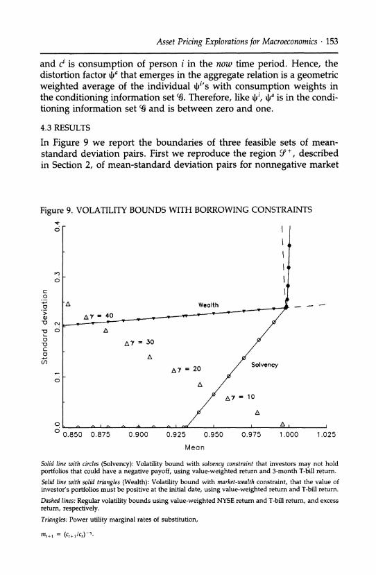
Asset Pricing Explorations for Macroeconomics ? 153
and ci is consumption of person i in the now time period. Hence, the distortion factor Ja that emerges in the aggregate relation is a geometric weighted average of the individual 4i's with consumption weights in the conditioning information set 3. Therefore, like 4i, qa is in the condi-
tioning information set J and is between zero and one.
4.3 RESULTS
In Figure 9 we report the boundaries of three feasible sets of mean- standard deviation pairs. First we reproduce the region S+, described in Section 2, of mean-standard deviation pairs for nonnegative market
Figure 9. VOLATILITY BOUNDS WITH BORROWING CONSTRAINTS
6
O
c) 0
0
a)
-0 0
0 -0 C
+t
0
Weolth = 40
A7 = 30
A
A7 = 20 Solvency
A
A
0.850 0.875 0.900 0.925 0.950
Mean
0.975 1.000 1.025
Solid line with circles (Solvency): Volatility bound with solvency constraint that investors may not hold portfolios that could have a negative payoff, using value-weighted return and 3-month T-bill return.
Solid line with solid triangles (Wealth): Volatility bound with market-wealth constraint, that the value of investor's portfolios must be positive at the initial date, using value-weighted return and T-bill return.
Dashed lines: Regular volatility bounds using value-weighted NYSE return and T-bill return, and excess return, respectively.
Triangles: Power utility marginal rates of substitution,
mt+1 = (ct+l/Ct)- .
154 COCHRANE & HANSEN
discount factors y. The second region, denoted 2 +, is the feasible set for the aggregate measures ma of intertemporal marginal rates of substi- tution that satisfy restriction (4.8) implied by the solvency constraint. The third region, denoted W +, is the feasible set for random variables ma that also satisfy the proportionality restriction (4.11). The regions are constructed using results from Luttmer (1991) and He and Modest (1991), and the mechanics underlying these constructions are provided in the next subsection. All three regions were constructed using the same quarterly value-weighted and T-bill return series used in many of our previous figures. Of course, both 3 + and M + are expanded ver- sions of the set Y +, and the feasible set W + is smaller than 3 + because it incorporates the additional proportionality restriction.
As before, we use triangles to record the mean-standard deviation pairs of aggregate measures of intertemporal marginal rates of substitu- tion for several choices of the power - y. Abstracting from sampling error, values of y in the vicinity of 40 are necessary to get into the more restrictive market-wealth region OW+, whereas values as low as 15 en- ter the solvency region 2. Reducing the subjective discount factor P to values less than one increases the range of y's that are inside the respective regions. Fairly sizable curvature values are still required to "resolve" the Equity-Premium Puzzle for either version of a borrowing constraint, especially for the market-wealth constraint. However, the Riskfree-Rate Puzzle now disappears.
In the case of the market-wealth constraint and say, y = 40, the distortion factor ECf required for (4.10) to be satisfied is on average about .87, which may seem implausibly large. Recall that 1 - 4i is shadow value of the market-wealth constraint for person i. Hence, 1 - Eqf is a (somewhat complicated) "average" shadow value where averaging takes place across consumers and over states of the world. When y = 40, this "average" shadow value is about 0.13 for quarterly data. Consequently, the presence of a market-wealth constraint elimi- nates the Riskfree-Rate Puzzle by presuming there is a high average shadow value for the constraint. Subsection 4.5 below includes a related reservation about the solvency constraint.
4.4 COMPUTATION
We now describe how to compute the boundaries of the solvency region + and market-wealth region W + reported in Figure 9. As indicated previously, Luttmer (1991) provided a general algorithm for calculating the lower envelope of 2 +. The algorithm is fairly easy to describe when there are only two original securities, each with a limited liability. Recall

Asset Pricing Explorations for Macroeconomics ? 155
in our application, we used the value-weighted and T-bill returns as our
payoffs, both of which we interpret as having limited liability. Let x denote a random vector formed by stacking these two returns,
and let P+ denote the cone of limited-liability payoffs that can be con- structed from constant-weighted portfolios:
P+ {p: p = c * x for c E R2, p 2 0}. (4.13)
Any ma that is less than or equal to y will assign a price to a payoff in P+ that is less than or equal to its market price:
E(map) ' E(yp) for all p in P+. (4.14)
Because portfolio payoffs outside of P+ are sometimes negative, the
price distortion for these payoffs is ambiguous in sign. Next, note that in exploring the ramifications of equation (4.14), it
suffices to look at the two edge portfolios, say, p, and P2. Any other payoff in P+ is a convex combination of these edges with nonnegative portfolio weights. Because the original two securities have nonnegative payoffs, each edge has a positive portfolio weight on one of these securi- ties and a nonpositive weight on the other.17 We normalize these edge payoffs so that their price is one, that is, they are returns, and we number them so that
Ep1 > Ep2. (4.15)
It turns out the boundary of ~ + has three segments. First, there is a horizontal segment at r(ma) = 0 from E(ma) = 0 to E(ma) = 1/Epl. This segment is present because for any constant ma between zero and 1/Epl, inequality (4.14) is satisfied for both p, and P2. Furthermore, as long as the constant is strictly less than 1/Ep1, the inequalities will be strict. When the constant is equal to 1/Ep1, (4.14) will hold with equality by construction for edge payoff pi. This is the point at which the second segment begins.
The second segment of the boundary of 3 + coincides with a segment
17. The payoffs we used are strictly positive for all dates in the sample. We approximated the edges by initially holding fixed the positive weight and adjusting the negative weight until the resulting portfolio payoff is zero at one sample point and positive at all other points. In practice, approximation of edges using the empirical distribution may be poor because upper and lower endpoints of these distributions may be hard to estimate.

156 . COCHRANE & HANSEN
of the boundary of feasible mean-standard deviation region YS for sto- chastic discount factors that correctly price p, (but not necessarily P2). The boundary of Yf touches the horizontal axis at the point (1/Ep1,O) because as was just mentioned, a constant discount factor 1/Ep1 prices p, correctly. Furthermore, any other frontier discount factor for YS will also be a frontier random variable for 2 + as long as (4.14) is satisfied for P2. Hence, to construct the second segment of the boundary of 2 +, we follow the right boundary of fi until we obtain a frontier discount factor that also just prices P2 correctly.
The third segment of the boundary of 3 + coincides with a segment of the boundary of the region S+, of stochastic discount factors that
price correctly all constant-weighted portfolios of value-weighted and T-bill returns. Such discount factors satisfy (4.14) with equality for all admissible payoffs.18
Consider next the boundary of W + . This construction follows He and Modest (1991) and is included here for completeness. Multiplying both sides of (4.11) by x, taking expectations (first conditioned on ' and then
unconditionally), we have
E(max) = (Eqf)q , where 0 < Efa ? 1. (4.16)
Consequently, for any ma satisfying equation (4.11), we can find a sto- chastic discount factor ma/Era that prices the payoffs in x correctly.
Because the means and standard deviations of scale multiples of ran- dom variables simply inherit the same scaling, the link between S + and W + is particularly simple. Scale all of the points in SD+ by arbitrary numbers between zero and one, that is, for any point in S+, the ray from the origin to this point is in W +. Notice from Figure 9 that the boundary of W + has two segments. One coincides with a portion of the boundary of S +, and the other coincides with a portion of the boundary of the analogous region constructed using the excess return of stocks over bonds.
4.5 USING AGGREGATES TO SHARPEN BOUNDS ON MARKET DISCOUNT FACTORS
There is a different way to use the information contained in the marginal rates of substitution based on aggregate data in the presence of bor- rowing constraints. Rather than weakening the volatility implications to
18. With more than two securities, one follows a natural generalization of the above procedure. One first locates the edges of the cone P+. Once they are located, one can use Luttmer's more general algorithm for computing the bounds with the short-sale constraints imposed on the edge payoffs.
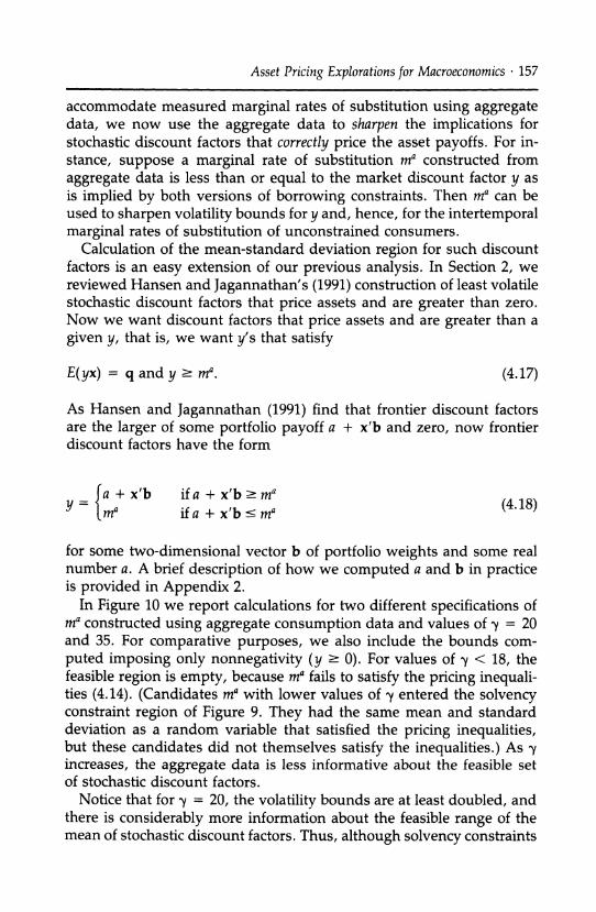
Asset Pricing Explorations for Macroeconomics * 157
accommodate measured marginal rates of substitution using aggregate data, we now use the aggregate data to sharpen the implications for stochastic discount factors that correctly price the asset payoffs. For in- stance, suppose a marginal rate of substitution ma constructed from
aggregate data is less than or equal to the market discount factor y as is implied by both versions of borrowing constraints. Then ma can be used to sharpen volatility bounds for y and, hence, for the intertemporal marginal rates of substitution of unconstrained consumers.
Calculation of the mean-standard deviation region for such discount factors is an easy extension of our previous analysis. In Section 2, we reviewed Hansen and Jagannathan's (1991) construction of least volatile stochastic discount factors that price assets and are greater than zero. Now we want discount factors that price assets and are greater than a given y, that is, we want y's that satisfy
E(yx) = q and y ma. (4.17)
As Hansen and Jagannathan (1991) find that frontier discount factors are the larger of some portfolio payoff a + x'b and zero, now frontier discount factors have the form
fa+x'b if a + x'b > ma y m if a + x'b ma (4.18)
for some two-dimensional vector b of portfolio weights and some real number a. A brief description of how we computed a and b in practice is provided in Appendix 2.
In Figure 10 we report calculations for two different specifications of ma constructed using aggregate consumption data and values of y = 20 and 35. For comparative purposes, we also include the bounds com- puted imposing only nonnegativity (y - 0). For values of y < 18, the feasible region is empty, because ma fails to satisfy the pricing inequali- ties (4.14). (Candidates ma with lower values of y entered the solvency constraint region of Figure 9. They had the same mean and standard deviation as a random variable that satisfied the pricing inequalities, but these candidates did not themselves satisfy the inequalities.) As y increases, the aggregate data is less informative about the feasible set of stochastic discount factors.
Notice that for y = 20, the volatility bounds are at least doubled, and there is considerably more information about the feasible range of the mean of stochastic discount factors. Thus, although solvency constraints
158 ? COCHRANE & HANSEN
loosen the implications of security market data for marginal rates of substitution computed from aggregate data, the data still pose a striking puzzle for the behavior of unconstrained consumers. Thus, even though models with solvency constraints weaken substantially the link between
aggregate consumption data and asset market returns, taken together the consumption and asset return data still imply rather startling impli- cations for the intertemporal marginal rates of substitution of the uncon- strained consumers.
4.6 EXTENSIONS
Recently, there has been a variety of work in asset pricing that seems well suited to guide empirical analyses of other market frictions. For instance, Prisman (1986), Jouni and Kallal (1991), and Luttmer (1991)
Figure 10 VOLATILITY BOUNDS FOR DISCOUNT FACTORS GREATER THAN A CANDIDATE
0
/
/ 7 = 20 / . 7 = 35
/
C 0
0 l
a) -0
L_ ~0 0Z c0 d 0
. /
cN
6
0.9950 0.9975 1.0000 1.0025
Mean
Solid line: Volatility bound using value-weighted NYSE and T-bill returns, for reference. Dashed and dotted lines: Minimum standard deviation of discount factors that (1) price the real value- weighted NYSE and T-bill returns (satisfy 1 = E(yx)), (2) are always greater than a candidate based on aggregate data, Yt+i 2 (Ct+l/c,)-Y; and (3) have the indicated mean.
" ..................."
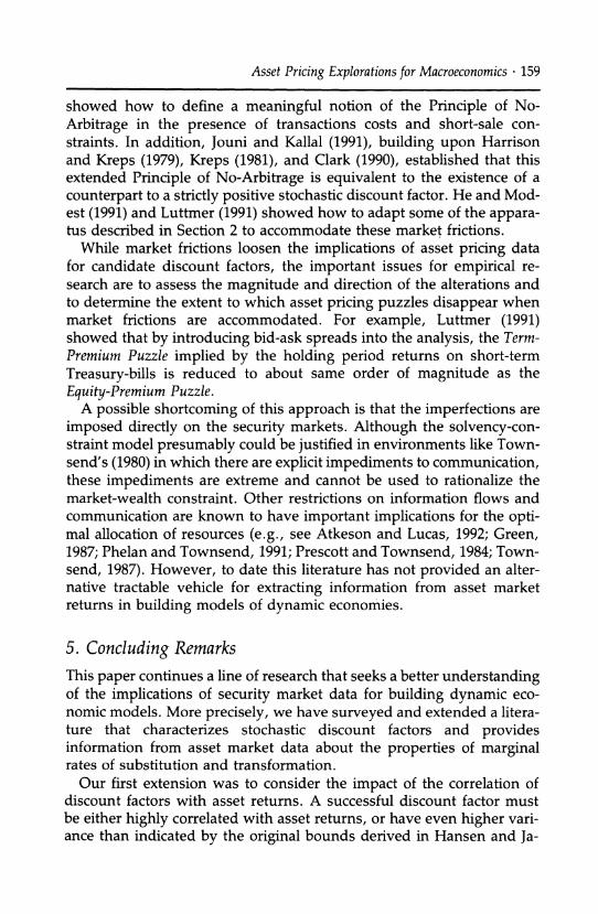
Asset Pricing Explorations for Macroeconomics ? 159
showed how to define a meaningful notion of the Principle of No-
Arbitrage in the presence of transactions costs and short-sale con- straints. In addition, Jouni and Kallal (1991), building upon Harrison and Kreps (1979), Kreps (1981), and Clark (1990), established that this extended Principle of No-Arbitrage is equivalent to the existence of a
counterpart to a strictly positive stochastic discount factor. He and Mod- est (1991) and Luttmer (1991) showed how to adapt some of the appara- tus described in Section 2 to accommodate these market frictions.
While market frictions loosen the implications of asset pricing data for candidate discount factors, the important issues for empirical re- search are to assess the magnitude and direction of the alterations and to determine the extent to which asset pricing puzzles disappear when market frictions are accommodated. For example, Luttmer (1991) showed that by introducing bid-ask spreads into the analysis, the Term- Premium Puzzle implied by the holding period returns on short-term
Treasury-bills is reduced to about same order of magnitude as the
Equity-Premium Puzzle. A possible shortcoming of this approach is that the imperfections are
imposed directly on the security markets. Although the solvency-con- straint model presumably could be justified in environments like Town- send's (1980) in which there are explicit impediments to communication, these impediments are extreme and cannot be used to rationalize the market-wealth constraint. Other restrictions on information flows and communication are known to have important implications for the opti- mal allocation of resources (e.g., see Atkeson and Lucas, 1992; Green, 1987; Phelan and Townsend, 1991; Prescott and Townsend, 1984; Town- send, 1987). However, to date this literature has not provided an alter- native tractable vehicle for extracting information from asset market returns in building models of dynamic economies.
5. Concluding Remarks This paper continues a line of research that seeks a better understanding of the implications of security market data for building dynamic eco- nomic models. More precisely, we have surveyed and extended a litera- ture that characterizes stochastic discount factors and provides information from asset market data about the properties of marginal rates of substitution and transformation.
Our first extension was to consider the impact of the correlation of discount factors with asset returns. A successful discount factor must be either highly correlated with asset returns, or have even higher vari- ance than indicated by the original bounds derived in Hansen and Ja-

160 . COCHRANE & HANSEN
gannathan (1991). Our second extension used conditioning information to split the unconditional variance of discount factors into two compo- nents: average conditional variance and variation in conditional means.
These two extensions refine previous characterizations of stochastic discount factors. Quarterly discount factors should be highly volatile (standard deviation at least .24 based on unconditional moments, .38 based on conditional moments), they should have a mean of about .998, they should be highly correlated with asset returns or have even higher variance, and most of their unconditional variation must be accounted for by average conditional variation rather than variation of conditional means. These characterizations may help in the further refinement of frictionless representative consumer models. Alternatively, we may be led to consider models with market frictions.
While market frictions loosen the implications of asset pricing data for candidate discount factors, the important issues for empirical re- search are to assess the magnitude and direction of the alterations and to determine the extent to which asset pricing puzzles disappear when market frictions are accommodated. Our analysis focused on two forms of frictions: solvency constraints and market-wealth constraints. These seemed to alleviate the puzzles to some extent. However, it appears that our estimated "average" shadow value of the market-wealth con- straint is implausibly high, and that the solvency constraint implies extreme volatility for the intertemporal marginal rates of substitution of the unconstrained consumers.
ACKNOWLEDGMENTS
In writing this paper we benefited greatly from conversations with John Campbell, Larry Epstein, John Heaton, Erzo Luttmer, Alex Taber, Grace Tsiang, Philippe Weil and Amir Yaron. Amir Yaron and Tim Conley provided expert research assistance. This research was partially supported by grants from the National Science Foundation.
REFERENCES
Abel, A. B. (1990). Asset prices under habit formation and catching up with the Joneses. American Economic Review 80:38-42.
Atkeson, A., and R. E. Lucas, Jr. (1992). On efficient distribution with private information. Review of Economic Studies 59:427-453.
Bekaert, G., and R. J. Hodrick (1992). Characterizing predictable components in excess returns on equity and foreign exchange markets. Journal of Finance 47:467-509.
Bewley, T. (1977). The permanent income hypothesis: A theoretical formulation. Journal of Economic Theory 16:252-292
.(1980). The optimum quantity of money. In Models of Monetary Economies. J. H. Kareken and N. Wallace (eds.), Federal Reserve Bank of Minneapolis, pp. 169-210.
Asset Pricing Explorations for Macroeconomics ? 161
Braun, P. (1991). Asset pricing and capital investment: Theory and evidence. Northwestern University manuscript.
Brown, D. P., and M. Gibbons. (1985). A simple econometric approach for utility-based asset pricing models. The Journal of Finance 40:359-381.
Burnside, C. (1991). Hansen-Jagannathan Bounds As Classical Tests of Asset Pricing Models. Queen's University manuscript.
Cecchetti, S. G., P. Lam, and N. C. Mark. (1992). Testing Volatility Restrictions on Intertemporal Marginal Rates of Substitution Implied by Euler Equations and Asset Returns. Ohio State University manuscript.
Clark, S. A. (1990). The valuation problem in arbitrage price theory. Journal of Mathematical Economics. Forthcoming.
Cochrane, J. H. (1991). Production-based asset pricing and the link between stock returns and economic fluctuations. Journal of Finance 46:207-234.
. (1992a). A cross-sectional test of a production-based asset pricing model. NBER Working Paper #4025.
. (1992b). Explaining the variance of price-dividend ratios. Review of Finan- cial Studies. 5:243-280.
Connor, G. (1984). A unified beta pricing theory. Journal of Economic Theory 34:13-31.
Constantinides, G. (1990). Habit formation: A resolution of the equity premium puzzle. Journal of Political Economy 98:519-543.
, and D. Duffie. (1991). Asset pricing with heterogeneous consumers: Good news and bad news. University of Chicago manuscript.
,and D. Duffie. (1992). Asset Pricing with Heterogeneous Consumers. University of Chicago manuscript.
Deaton, A. (1991). Saving and liquidity constraints. Econometrica 59:1221-1248. Epstein, L., and S. Zin. (1991). Substitution, risk aversion, and temporal behav-
ior of consumption and asset returns II: An empirical analysis. Journal of Politi- cal Economy 99:263-286.
Fama, E. F. (1970). Efficient capital markets: A review of theory and empirical work. Journal of Finance 25:383-417.
. (1991). Efficient capital markets: II. Journal of Finance 46:1575-1617. Ferson, W. E., and G. M. Constantinides. (1991). Habit persistence and durabil-
ity in aggregate consumption. Journal of Financial Economics 29:199-240. Gallant, R., L. P. Hansen, and G. Tauchen. (1990). Using conditional moments
of asset payoffs to infer the volatility of intertemporal marginal rates of substi- tution. Journal of Econometrics 45:141-179.
Green, E. (1987). Lending and the smoothing of uninsurable income. In Contrac- tual Arrangements for Intertemporal Trade. In E. C. Prescott and N. Wallace (eds.), Minneapolis: University of Minnesota Press.
Grossman, S. J., and R. J. Shiller. (1981). The determinants of the variability of stock market prices. American Economic Review 71:222-227.
Hansen, L. P. (1982). Large sample properties of generalized method of mo- ments estimators. Econometrica 50:1029-1054.
, J. Heaton, and R. Jagannathan. (1992). Econometric Evaluation of Inter- temporal Asset Pricing Models. Forthcoming.
,and R. Jagannathan. (1991). Implications of security market data for models of dynamic economies. Journal of Political Economy 99:225-262.
, and . (1992). Assessing specification errors in stochastic discount factor models. Manuscript.
162 * COCHRANE & HANSEN
,and S. F. Richard. (1987). The role of conditioning information in deduc- ing testable restrictions implied by dynamic asset pricing models. Econometrica 55:587-613.
, and K. J. Singleton. (1982). Generalized instrumental variables estima- tion of nonlinear rational expectations models. Econometrica 50:1269-1286.
Harrison, M. J., and D. M. Kreps. (1979). Martingales and arbitrage in multi- period securities markets. Journal of Economic Theory 20:381-408.
Hayashi, F. (1987). Tests for liquidity constraints: A critical survey and some new observations. Advances in Econometrics, Fifth World Congress 2:91-120.
He, H., and D. M. Modest. (1991). Market frictions and consumption-based asset pricing. Manuscript. University of California, Berkeley.
Heaton, J. (1991). An empirical investigation of asset pricing with temporally dependent preference specification, MIT Sloan School Working Paper #3245- 91-EFA.
Hindy, A. (1992). Viable prices in financial markets with solvency constraints. Stanford University manuscript.
Jouni, E., and H. Kallal (1991). Martingales, arbitrage and equilibrium in securi- ties markets with transaction costs. University of Chicago manuscript.
Knez, P. J. (1991). Pricing money market securities with stochastic discount factors. University of Wisconsin manuscript.
Kocherlakota, N. R. (1990). On the discount factor in growth economies. Journal of Monetary Economics 25:43-48.
Kreps, D. M. (1981). Arbitrage and equilibrium in economies with infinitely many commodities. Journal of Mathematical Economics 8:15-35.
Kydland, F. E., and E. C. Prescott. (1982). Time to build and aggregate fluctua- tions. Econometrica 50:1345-1370.
Lintner, J. (1965). Valuation of risk assets and the selection of risky invest- ments in stock portfolios and capital budgets. Review of Economics and Statistics 47:13-27.
Long, J. B., Jr., and C. I. Plosser. (1983). Real business cycles. Journal of Political Economy 91:39-69.
Luttmer, E. G. J. (1991). Asset pricing in economies with frictions. University of Chicago manuscript.
MacKinlay, A. C., and M. P. Richardson. (1991). Using generalized method of moments to test mean-variance efficiency. The Journal of Finance 46:511-527.
Mankiw, N. G. (1986). The equity premium and the concentration of aggregate shocks. Journal of Financial Economics 17:211-219.
, and S. P. Zeldes. (1991). The consumption of stockholders and non- stockholders. Journal of Financial Economics 29:97-112.
Manuelli, R., and T. J. Sargent (1992). Alternative monetary policies in a turn- pike economy. Manuscript.
Mehra, R., and E. C. Prescott (1985). The equity premium puzzle: A solution? Journal of Monetary Economics 22:133-136.
Mossin, J. (1968). Equilibrium in a capital asset market. Econometrica 34:768-783. Newey, W., and K. D. West. (1987). A simple positive semi-definite, hetero-
skedasticity and autocorrelation consistent covariance matrix. Econometrica 55:703-708.
Phelan, C., and R. Townsend. (1991). Computing multi-period, information constrained optima. Review of Economic Studies 58:853-881.
Prescott, E., and R. Townsend. (1984). Pareto optima and competitive equilibria with adverse selection and moral hazard. Econometrica 52:21-46.

Asset Pricing Explorations for Macroeconomics . 163
Prisman, E. Z. (1986). Valuation of risky assets in arbitrage free economies with frictions. The Journal of Finance 41:545-559.
Rietz, T. A. (1988). The equity risk premium: A solution. Journal of Monetary Economics 22:117-131.
Roll, R. (1977). A critique of the asset pricing theory's tests: Part I: On past and potential testability of the theory. Journal of Financial Economics 4:129-176.
Ross, S. A. (1976). The arbitrage theory of capital asset pricing. Journal of Eco- nomic Theory 13:321-360.
Rubinstein, M. (1976). The valuation of uncertain income streams and the pric- ing of options. Bell Journal of Economics 7:407-425.
Runkle, D. E. (1991). Liquidity constraints and the permanent income hypothe- sis: Evidence from panel data. Journal of Monetary Economics. Forthcoming.
Santos, M., and M. Woodford. (1992). Rational speculative bubbles. University of Chicago Manuscript.
Scheinkman, J. A. (1989). Market incompleteness and the equilibrium valuation of assets. In Financial Markets and Incomplete Information: Frontiers of Modern Financial Theory, Vol. 1, S. Bhattacharya and G. M. Constantinides (eds.). Totowa, NJ: Littlefield and Rowman Pub.
, and L. Weiss. (1986). Borrowing constraints and aggregate economic activity. Econometrica 54:23-46.
Sharpe, W. F. (1964). Capital asset prices: A theory of market equilibrium under conditions of risk. Journal of Finance 19:425-442.
Snow, K. N. (1991). Diagnosing asset pricing models using the distribution of asset returns. Journal of Finance 46:955-984.
Townsend, R. (1980). Models of money with spatially separated agents. In Mod- els of Monetary Economics, J. H. Kareken and N. Wallace (eds.), pp. 265-303, Federal Reserve Bank of Minneapolis.
. (1987). Arrow-Debreu programs as microfoundations of macroeconom- ics. In Advances in Economic Theory, Fifth World Congress, T. F. Bewley (ed.), Cambridge University Press, pp. 379-428.
, and N. Wallace. (1987). Circulating private debt: An example with a coordination problem. In Contractual Arrangements for Intertemporal Trade, Vol. 1, pp. 105-120. Minnesota Studies in Macroeconomics.
Weil, P. (1989). The equity premium puzzle and the risk free rate puzzle. Journal of Monetary Economics 24:401-421.
Zeldes, S. (1989). Consumption and liquidity constraints: An empirical investi- gation. Journal of Political Economy 97:305-346.
APPENDIX 1 In this appendix we provide more information about our method for
computing Figure 5. The aim is to minimize E[var(yl I)] subject to a constraint that var[E(ylqg)] = c for some valid positive number c. First, write the expected conditional variance of y as
E[var(y I)] = E(y2) - E{[E(y I)]2}, (A.1)
and the variance of E(ylIg) as

164 * COCHRANE & HANSEN
var[E(y lI)] = E[E(y| )2] - (Ey)2. (A.2)
Then the associated Lagrangian is given by
? = E(y2) - (1 + X)E{[E(y|S)]2} + X(Ey)2. (A.3)
Finally, as argued in the text, use the representation of the conditional mean-standard deviation frontier for stochastic discount factors given in Gallant, Hansen, and Tauchen (1990):
Yw = P* + we*, (A.4)
where w E ', p* is the minimum second moment stochastic discount factor and e* is the error in the conditional projection of a unit payoff onto the vector x of payoffs used in an econometric analysis. Explicit formulas are given in Gallant, Hansen, and Tauchen. In solving the constrained minimization problem it suffices to look at discount factors of the form (A.4). Hence, we only need to choose w.
To derive the first-order conditions, we follow the usual practice of perturbing the optimal w in any arbitrary direction in the conditioning information set 'S. The optimal (real) coefficient on that perturbation must be zero for all such directions. This results in the following first- order conditions for the optimization:
E(ywe*l6) - (1 + X)E(ywJI)E(e*I)) + X(Eyw)E(e*l6) = 0. (A.5)
Because e* is the conditional projection error of a unit payoff onto the vector x of payoffs, the corresponding projection is 1 - e*. Hence, e* is conditionally orthogonal to 1 - e*, and
E[(e*)2 | ] = E(e*I ). (A.6)
It follows from (A.4) and (A.6) that
E(ywe*l ) = wE[(e*)2 1] = wE(e*lI). (A.7)
Substituting equation (A.7) into equation (A.5) and dividing by E(e* IC) gives
w - (1 + X)E(ywl<) + X(Eyw) = 0 (A.8)
Solving equations (A.8) and (A.4) for w gives the solution to the problem.

Comment. 165
APPENDIX 2
In this appendix we briefly describe an algorithm that we used to con- struct the volatility bounds reported in Figure 10. The algorithm is very similar but not identical to one suggested by Hansen and Jagannathan (1992) for computing specification error bounds.
Step 1: Transform prices so that the new pricing formula is
E[(y - ma)x] = q where q - q - E(max).
Step 2: Find the arbitrage bounds for pricing unit payoff with the q prices.
Step 3: Augment x with a unit payoff and augment q with a corre- sponding ^ price of a unit payoff within the arbitrage bounds. Setting a ^ price for a unit payoff determines the mean of y via:
Ey = *r(1) + Ema.
Step 4: Find the arbitrage bounds for pricing ma using the augmented payoffs and prices. For each price, find the minimum norm nonnegative stochastic discount factor by solving the dual problem in Hansen and Jagannathan (1991). Note that
E(y2) = E[(y - ma)2] + 2E[(y - ma)ma] + E[(ma)2].
By fixing the price assignment to ma, we fix the middle term, and the third term is fixed by our measure of ma. Hence, we minimize the left side by minimizing the first term. The dual problem in Hansen and Jagannathan (1991) is designed to minimize E[(y - ma)2] by choice of a nonnegative value of (y - ma) subject to the pricing restriction. Finally, minimize E(y2) by choice of the price assignment to ma.
Notice that step 3 provides a mean and step 4 the corresponding second moment bound. Since the mean is fixed in step 4, we obtain a corresponding volatility bound. Steps 3 and 4 must be repeated for all A price assignments to a unit payoff within the arbitrage bounds.
Comment JOHN Y. CAMPBELL Princeton University and NBER
This paper has all the merits, and some of the disadvantages, of a sys- tematic methodology and a tight focus. It reminds me of a famous poem This paper has all the merits, and some of the disadvantages, of a sys- tematic methodology and a tight focus. It reminds me of a famous poem