australia’s carbon tax - institute for energy...
TRANSCRIPT

AN ECONOMIC EVALUATION | 1
Australia’s Carbon Tax: An Economic Evaluation
by Dr. Alex Robson, PhD
Department of Accounting, Finance and Economics
Griffith University, Brisbane, Australia
September 2013

AUSTRALIA’S CARBON TAX

AN ECONOMIC EVALUATION | 1
Table of Contents
Executive Summary ......................................................................................................................5
1. Introduction ..........................................................................................................................11
2. History of the Carbon Tax ....................................................................................................12
2.1. The Shergold Report (2007) ............................................................................................12
2.2. The Garnaut Report (2008) and the Carbon Pollution Reduction Scheme (CPRS) (2009) ..................................................................................14
2.3. Carbon Taxes versus Cap and Trade Schemes: The Standard Treatment in the Literature ........................................................................15
3. Policy Framework and Key Parameters..............................................................................18
3.1. Development of the Tax ................................................................................................18
3.2. Coverage: Who Pays?....................................................................................................18
3.3. Abatement Target and Sources of Abatement ..............................................................19
3.4. The Price Floor and Price Ceiling ..................................................................................19
3.5. Other Policies ................................................................................................................21
3.5.1. Complementary Emissions Reduction Policies..................................................21
3.5.2. Household Compensation..................................................................................22
3.5.3. Free Permits ......................................................................................................22
4. The Economic Costs of Australia’s Carbon Tax ................................................................23
4.1. The Carbon Tax and Australia’s Exports ........................................................................23
4.2. The Interaction Between the Carbon Tax and Other Policies ........................................25
4.2.1. Complementary Emissions Reduction Policies..................................................25
4.2.2. The Effects of Household Assistance and Income Tax Changes ......................25
4.3. International Linking and Restrictions on International Trade ........................................28
4.3.1. The Gains from International Trade in Permits ..................................................28
4.3.2. Constraints on Overseas Permit Purchases ......................................................29
AN ECONOMIC EVALUATION | 1

2 | AUSTRALIA’S CARBON TAX
4.4. Dynamic (In)efficiency ....................................................................................................31
5. Economic and Fiscal Effects................................................................................................32
5.1. Gross Domestic Product (GDP) Losses ........................................................................32
5.2. GDP Costs per Tonne of Abatement..............................................................................34
5.3. Business Costs, Profitability and Carbon Leakage........................................................35
5.4. Real Wages and Unemployment....................................................................................37
5.5. Consumer Prices............................................................................................................39
5.6. Fiscal Effects ..................................................................................................................41
5.7. Effect on CO2-e Emissions ............................................................................................43
5.7.1. Overall Emissions ..............................................................................................43
5.7.2. Electricity Sector Emissions ..............................................................................43
6. Conclusions: Policy Lessons from the Australian Experience ........................................47
References....................................................................................................................................50
Appendices ..................................................................................................................................51
Endnotes ......................................................................................................................................56

AN ECONOMIC EVALUATION | 3
List of Figures
Figure 2.1: Marginal Costs and Benefits of CO2-e Abatement ....................................................12
Figure 2.2: A Cap and Trade Scheme ..........................................................................................13
Figure 2.3: Transaction Costs in a Cap and Trade Scheme ..........................................................13
Figure 2.4: Summary of the Legislative History of the Carbon Tax ..............................................15
Figure 2.5: Efficiency Losses from a Carbon Tax and a Cap and Trade Scheme When Marginal Costs are Unexpectedly High ..............................................16
Figure 3.1: Sources of Cumulative Abatement Relative to Business as Usual Projections, 2013-2050 ................................................................................19
Figure 3.2: Baseline Permit Prices, Price Ceiling Path and Price Floor Path Under the Original CEF Policy ............................................................................20
Figure 3.3: Welfare Effects of a Price Floor and Price Ceiling ......................................................21
Figure 4.1: Peters and Hertwich (2008) Estimates of the Balance of Emissions in Trade ............24
Figure 4.2: The Costs of a Mandatory Renewable Energy Target ................................................25
Figure 4.3: The “Tax Interaction Effect”: The Welfare Effects of a Pigouvian Tax when there is a Pre-Existing Distortion in a Related Market ......................................26
Figure 4.4: International Trade in Emissions Permits ....................................................................29
Figure 4.5: Domestic Emissions and Abatement with Free Trade in Permits................................29
Figure 4.6: Domestic Emissions and Abatement Under Australia's CEF Policy to 2020..............30
Figure 4.7: Carbon Price Projections, 2012-13 to 2019-20 ..........................................................31
Figure 5.1: Present Value of Projected Economic Costs of Australia's Carbon Tax to 2050 ........33
Figure 5.2: Average and Incremental Costs of Abatement, Relative to Business as Usual Emissions....................................................................34
Figure 5.3: Sectoral Shares of Total Business Electricity Use, 2011-12 ......................................35
Figure 5.4: Carbon Leakage in an Import-Competing Industry ....................................................36
Figure 5.5: Annual Reduction in Real Wages Versus Annual Reduction in GDP Under the Carbon Tax, Relative to Baseline, 2013-2020................................37

4 | AUSTRALIA’S CARBON TAX
Figure 5.6: Unemployment in Australia, July 2012 to July 2013 ..................................................38
Figure 5.7: Inflation-Adjusted Household Electricity Prices, 1980 to 2013 ..................................40
Figure 5.8: Expected Cumulative Fiscal Impact of the Carbon Tax and Associated Policies, 2011-12 to 2014-15 ........................................42
Figure 5.9: Initial Estimates and Revisions of Carbon Tax Revenue, 2012-13 to 2016-17 ..........43
Figure 5.10: Government Projections of Australia's Domestic CO2-e Emissions Under the Carbon Tax, 2013-2050..............................................44
Figure 5.11: Australia’s Electricity CO2-e Emissions, 2002-2012 ................................................45
Figure 5.12: Australia's total CO2-e emissions, Seasonally Adjusted Weather Normalised, 2002-2013..............................................................................46
List of Tables
Table 3.1: Allocation of Free Permits to Emissions Intensive Trade Exposed Industries ............22
Table 4.1: New Statutory Income Tax Rates, Old EMTRS and New EMTRs ..............................28
Table 5.1: Estimated GDP Costs of Policy Commitments Under the Copenhagen Accord........32
Table 5.2: Estimated Effect of the Carbon Tax on Wholesale Electricity Prices to 2050 ............39
Table 5.3: Estimated Contribution of the Introduction of the Carbon Tax and Other Green Schemes to a Typical Annual Household Electricity Bill, Qld and NSW ........................................................41
July 2012Carbon tax beginsFebruary 2011
Governmentannounces proposedarchitecture ofcarbon tax
August 2010Governmentpromises not to introduce carbon tax
April 2010Governmentwithdraws cap and tradelegislation and commits not to introduce scheme before the end of 2012
May 2009Cap and tradelegislation introduced.Scheme to begin on July 1 2010
AN ECONOMIC EVALUATION | 5
Executive Summary
Australia has implemented a carbon tax, and it is failing to deliver any of its promised benefits. Its failures
have made the tax a highly politicized issue, and may provide lessons for other nations. The tax, which is
currently set at $24.151 is the central component of the Australian Government’s climate change policy.
The tax applies directly to around 370 Australian businesses2 and was originally designed as a precursor
to a “cap and trade” scheme, with the transition to a flexible price originally (and currently) scheduled to
take place on July 1, 2015.
This report, commissioned by the Institute for EnergyResearch, evaluates Australia’s carbon tax experienceand draws lessons for policymakers in the UnitedStates and other jurisdictions, who may beconsidering following the Australian example andimplementing their own carbon taxes or cap and tradeschemes. The analysis establishes a number of keypoints, which are summarised below.
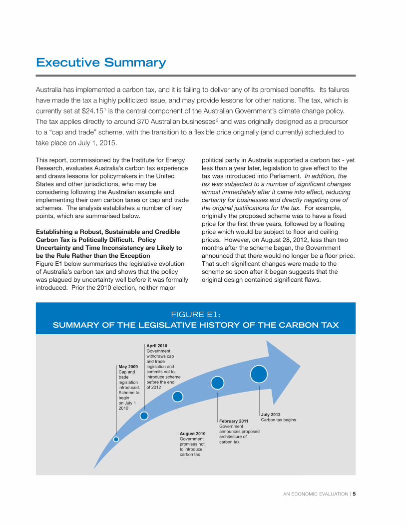
Establishing a Robust, Sustainable and CredibleCarbon Tax is Politically Difficult. PolicyUncertainty and Time Inconsistency are Likely tobe the Rule Rather than the ExceptionFigure E1 below summarises the legislative evolutionof Australia’s carbon tax and shows that the policywas plagued by uncertainty well before it was formallyintroduced. Prior the 2010 election, neither major
political party in Australia supported a carbon tax - yetless than a year later, legislation to give effect to thetax was introduced into Parliament. In addition, thetax was subjected to a number of significant changesalmost immediately after it came into effect, reducingcertainty for businesses and directly negating one ofthe original justifications for the tax. For example,originally the proposed scheme was to have a fixedprice for the first three years, followed by a floatingprice which would be subject to floor and ceilingprices. However, on August 28, 2012, less than twomonths after the scheme began, the Governmentannounced that there would no longer be a floor price.That such significant changes were made to thescheme so soon after it began suggests that theoriginal design contained significant flaws.
FIGURE E1:SUMMARY OF THE LEGISLATIVE HISTORY OF THE CARBON TAX

Sep1980
Sep1982
Sep1984
Sep1986
Sep1988
Sep1990
Sep1992
Sep1994
Sep1996
Quarter
Sep1998
Sep2000
Sep2002
Sep2004
Sep2006
Sep2008
Sep2010
Sep2012
Carbon TaxIntroduced
0
0.5
1
1.5
2
2.5
Inde
x of
Hou
seho
le E
lect
ricity
Pric
es (S
ep 1
980=
1)
6 | AUSTRALIA’S CARBON TAX
Despite the carbon tax passing both the House ofRepresentatives and the Senate and becoming law,political and popular support for the policy has beenweak. Recently the Australian Government hasproposed further major changes to the tax,announcing its desire to move earlier towards a capand trade scheme, with the new transition takingplace on July 1, 2014. However, legislation to giveeffect to this proposed change has not yet beenintroduced into Parliament; and in any case, it isunclear whether such legislation would actually bepassed.3
As a result, there is still a great deal of uncertaintysurrounding the future status of the carbon tax.Depending on the result of the forthcoming election,the tax may either remain in place and transition tocap and trade in 2015, or it may move to a cap andtrade scheme in 2014, or it may be abolishedcompletely.
In Assessing the Case for a Carbon Tax or Cap andTrade Scheme, the Incremental Net Benefits of AllFeasible Policy Options Were Not Estimated. One reason for the lack of robustness of the carbontax policy is that its development followed a flawedpolicy process. The role of climate change policy isnot to assess the possible damage of climate change,but rather to focus on the incremental net benefits ofpossible policy options. A central tenet of goodeconomic policymaking is that a full cost benefitanalysis (CBA) should be undertaken, weighing up thegains and losses across a wide range of policyalternatives so that political decision-makers can bebetter informed of the economic effects of variousoptions. Sensitivity analysis should be undertaken inorder to determine the extent to which the results ofsuch analysis depend on modelling assumptions andother inputs. If sensitivity analysis shows that aproposed policy’s estimated net benefits vary wildly
FIGURE E2: INFLATION-ADJUSTED HOUSEHOLD ELECTRICITY PRICES, 1980 TO 2013

720
700
680
660
640
620
600
580
560
540
Carbon Tax Introduced
Pers
ons
Une
mpl
oyed
(Tho
usan
ds)
July2011
Sep2011
Nov2011
Jan2012
Mar2012
May2012
July2012
Sep2012
Nov2012
Jan2013
Mar2013
May2013
July2013
Month
AN ECONOMIC EVALUATION | 7
with assumptions, the policy should be treated with agreat deal of care and probably rejected on thegrounds that it is unlikely to result in net benefits.
Whilst a number of Government-commissionedreports attempted to examine the economic costs ofcarbon taxes and emissions trading schemes, theincremental net benefits of the policy were neverassessed. In other words, costs and benefits werenever compared. Instead, Government-sponsoredreports purported to measure benefits by examiningthe possible future damage that may be caused byclimate change in Australia. But estimating thesecosts is not the same as estimating the benefits ofvarious policies. In particular, there was never anassessment of the incremental net benefits toAustralia of limiting emissions, versus other measuressuch as adaptation. The Australian debate has alwaysbeen framed as limiting emissions on the one hand,versus doing nothing on the other.
In addition, the Government’s quantitative modellingof the costs made a number of highly unrealisticassumptions and lacked transparency (Ergas andRobson, 2012). This made it impossible for neutralthird parties to replicate and evaluate the results, ormodify the assumptions to test the robustness of theresults.
The Cumulative Economic Costs of Carbon Taxesor Cap and Trade Schemes are Likely to beSubstantial Over the Long Term, with LowerDiscount Rates Resulting in Higher CumulativeCosts in Present Value Terms Under the carbon tax, most of the abatement thatAustralia will take credit for over the period to 2050will be undertaken overseas, with Australianbusinesses paying their foreign counterparts to reduceemissions. Nevertheless, the tax will have significanteconomic costs. So far the main economic effect ofthe tax has been to increase energy prices (particularly
FIGURE E3: UNEMPLOYMENT BEFORE AND AFTER THE INTRODUCTION OF THE CARBON TAX

Dec2002
Jun2003
Dec2003
Jun2004
Dec2004
Jun2005
Dec2005
Jun2006
Dec2006
Jun2007
Dec2007
Quarter
Jun2008
Dec2008
Jun2009
Dec2009
Jun2010
Dec2010
Jun2011
Dec2011
Jun2012
Dec2012
0
125
130
135
140
145
Emissions since the introduction of the carbon tax
Qua
rter
ly C
O2-
e Em
issi
ons
(Mt)
8 | AUSTRALIA’S CARBON TAX
electricity costs) for households and businesses (seeFigure E2). According to the Australian Industry Group(AIG), energy cost increases have averaged 14.5 percent for businesses as a result of the carbon tax,whilst TD Securities and the Melbourne Institute foundthat due to the introduction of the carbon tax, theprice of electricity for households rose by 14.9 percent. The increase in household electricity prices afterthe carbon tax was introduced was the highestquarterly increase on record.
The Government’s own modelling (which, as the reportdiscusses, are likely to have underestimated the costsof the tax) indicates that Australia’s Gross DomesticProduct (GDP) will be lower than it otherwise would befor every year that the tax is in place. Depending onthe discount rate used, the present value of these costscould be as high as 83 per cent of current AustralianGDP, or $1.25 trillion. The carbon tax has been
FIGURE E4: AUSTRALIA'S TOTAL CO2-E EMISSIONS, SEASONALLY ADJUSTED WEATHER NORMALISED, 2002-2013
directly linked to a number of business closures and joblosses, with overall unemployment rising significantlysince the tax was introduced (see Figure E3).
Furthermore, government data shows that the tax hasnot reduced the level of Australia’s domesticallyproduced CO2-e emissions (Figure E4). This is notsurprising, since under the carbon tax Australia’sdomestic emissions are not expected to fall belowcurrent levels until 2045.
Carbon Leakage is Likely and will Create EconomicCosts with no Offsetting Environmental BenefitOverall, Australia’s exports are relatively emissionsintensive. Hence a carbon tax is likely to increase thecost of exports, whose prices are largely determinedon world markets. There is little opportunity forAustralian export industries to pass on the increasesin costs that are due to the carbon tax. In other

35,000
30,000
25,000
20,000
15,000
10,000
5,000
0
-5,000
-10,000
$24,470 million
$3,300 million -$15,356 million
-$9,222 million
$-3,192 million
Revenue frompermit sales
Revenue from othermeasures
and fuel taxcredit
HouseholdAssistance
FreePermits
Overall Fiscal Impact-4,380 million
OtherPrograms
$ m
illio
n
Measure
AN ECONOMIC EVALUATION | 9
FIGURE E5: EXPECTED CUMULATIVE FISCAL IMPACT OF THE CARBON TAX AND ASSOCIATED POLICIES, 2011-12 TO 2014-15
words, the effect of the carbon tax on Australia’semissions-intensive, trade-exposed industries issimilar to a tax on exports or a tax on import-competing industries. Providing free permits to theseindustries does not alter marginal incentives.Domestic emissions in these industries may fall after acarbon tax is imposed, but that cannot be counted asan environmental gain if the ultimate effect is that thebusinesses shut down and emissions simply riseoverseas. The net effect will be a pure deadweightcost to the Australian economy.
Fiscal Impacts are Likely to be Uncertain, withboth Carbon Taxes and Cap and Trade SchemesAdding to Existing Revenue Volatility Due to the structure of the carbon tax andaccompanying policies, a sizeable fiscal gap hasopened up between the revenues generated by thetax on the one hand, and the increases in government
spending and tax cuts that accompanied the schemeon the other. A significant proportion of compensationpayments were “locked in”, whilst revenue from thetax is likely to be lower than originally anticipated.Hence the introduction of the tax, together with otherpolicies, is likely to worsen Australia’s budget bottomline going forward, leading to higher deficits andhigher public debt than would otherwise have beenthe case.
Attention Needs to be Paid to the Effects andCosts of “Complementary” Policies, Which AreLikely to Result in Efficiency Losses Rather thanEfficiency Gains, Compounding any NegativeEffects of a Carbon Tax or Cap and Trade SchemeTable E1 below shows that the carbon tax, togetherwith other green schemes, now account for asignificant portion of a typical Australian household’selectricity bills. Proponents of carbon taxes have

TABLE 2: INCREASED OUTPUT FROM OPENING FEDERAL LANDS($ MILLIONS ANNUALLY)
QLD (2012-13) NSW (2013-14)
RENEWABLE ENERGY TARGET $102 $107
SOLAR BONUS SCHEME/OTHER SCHEMES $67 $53
CARBON TAX $190 $172
TYPICAL HOUSEHOLD BILL $1900 $2073
GREEN SCHEMES/TOTAL 19 PER CENT 16 PER CENT
10 | AUSTRALIA’S CARBON TAX
pointed to several kinds of efficiency gains that mayaccompany such taxes. It is often claimed, forexample, that imposing a carbon tax allows policymakers to eliminate other, more costly“complementary” measures that are designed toreduce emissions, such as green subsidies (eg forsolar and wind power), renewable energy targets, andso on.
However, these efficiency gains are unlikely tomaterialise in Australia’s case: the complementarymeasures have remained in Australia after the carbontax was put in place. To make matters worse, newcomplementary measures have been introducedwhich will likely increase economic costs. Hence anyhypothetical efficiency gains that may have occurredas a result of eliminating other programs remain justthat: hypothetical.
TABLE E1: ESTIMATED CONTRIBUTION OF THE INTRODUCTION OF THE CARBON TAX AND OTHER GREEN SCHEMES TO A TYPICAL
ANNUAL HOUSEHOLD ELECTRICITY BILL, QLD AND NSW
The “Double Dividend” is Elusive in Theory andDifficult to Achieve in PracticeCarbon tax proponents also argue that carbon taxrevenue can be “recycled” and used to reducemarginal income tax rates, thus providing a “doubledividend.” The report also shows how the doubledividend hypothesis is a dubious proposition in theory,due to the interaction between the carbon tax and theexisting tax system (particularly personal income taxesand corporate taxes). In addition, as part of thehousehold compensation package for the carbon tax,the Australian Government lowered some averageincome tax rates but actually increased marginal taxrates for around 2 million taxpayers. This increase inmarginal tax rates is exactly the opposite policy ofwhat a Government would do if it were trying tocapture a “double dividend” from environmentaltaxation. In practice, therefore, there has been nodouble dividend from Australia’s carbon tax.
ConclusionPoor policy processes tend to lead to poor policyoutcomes. Australia’s carbon tax experience providesa number of important lessons in how not to go aboutimplementing sensible climate change policy.Although a number of Government reports examinedthe possible costs of the carbon tax, none of themassessed the incremental net benefits of the policy.For a variety of reasons, it is unlikely that Australia’scarbon tax will achieve “abatement at least cost.” Themost significant complementary climate changepolicies have remained in place after the introductionof the tax, and a range of new, costly measures wereintroduced to accompany the policy. These factorshave weakened—perhaps fatally—the economic casefor Australia’s carbon tax.
Overall, Australia’s exports are
relatively emissions intensive. Hence a
carbon tax is likely to increase the cost
of exports, whose prices are largely
determined on world markets.

AN ECONOMIC EVALUATION | 11
I. Introduction
Australia’s carbon tax, which came into effect on July 1, 2012 and is currently set at $24.15, covers a
broad range of industry sectors and categories of carbon dioxide equivalent (CO2-e) emissions. The tax is
a fixed price emissions permit system, and is legislated to move to a full “cap and trade” or flexible
emissions price scheme in 2015, with Australian firms permitted to buy permits from the European Union.
The stated purpose of the tax is to reduce Australia’s CO2-e emissions below projected “business as
usual” levels. Slightly less than half of the expected CO2-e abatement in the period to 2050 is expected to
occur as a result of domestic reductions in emissions, with the most abatement being sourced from
purchases of overseas permits.
Despite the carbon tax passing the House ofRepresentatives and the Senate and becoming law,political and popular support for the policy has beenweak. Recently the Australian Government hasproposed to move earlier towards an internationallylinked cap and trade scheme, in July 2014. However,legislation to give effect to this proposed change hasnot yet been introduced into Parliament. In any case,it is unclear whether such legislation—should it beintroduced—would even pass.4
As a result, there is a great deal of uncertaintysurrounding the future status of the tax. Dependingon the outcome of the forthcoming Australian election(which will be held on September 7), the tax mayeither (i) remain in place and transition to cap andtrade in 2015 (as originally planned); or (ii) it maymove earlier to a cap and trade scheme in 2014; or(iii) it may be abolished altogether.
This report evaluates the carbon tax in terms of policyprocess, policy design, and economic outcomes.The report is structured as follows. Section 2 outlinesthe policy history behind the carbon tax, and some ofthe legislative background to the current scheme, aswell as reviewing some of the basic economicarguments that have been made to justify theintroduction of the tax. Section 3 outlines the keyeconomic features of the scheme. Section 4examines the economic costs of the tax, and explainswhy it is unlikely that the Australian Government’spolicy will “achieve abatement at least cost.” Section5 examines the economic and fiscal effects of thecarbon tax. Section 6 concludes by outlining themain policy lessons from the Australian experience.
Despite the carbon tax passing the House of Representatives
and the Senate and becoming law, political and popular support for
the policy has been weak.

12 | AUSTRALIA’S CARBON TAX
2. History of the Carbon Tax
The political history of Australia’s carbon tax began with the Prime Ministerial Task Group on Emissions
Trading (more popularly known as the Shergold Report after its main author), which was released in mid
2007.5 This Task Group advised “on the nature and design of a workable global emissions trading system
in which Australia would be able to participate.” In response to the Shergold report, then Prime Minister
John Howard announced on July 17 that a “cap and trade” system would be introduced in Australia. The
scheme was planned to be operational possibly in 2011, and no later than 2012.6
The Shergold Report appealed to some standardanalysis and results from basic welfare economics tojustify its recommendation to introduce a cap andtrade scheme, arguing that emissions generateexternal costs and that the market supplies too large avolume of emissions relative to the efficient level.Consider, for example, Figure 2.1 below, which plotsthe aggregate marginal costs and benefits ofabatement in the case where there is completecertainty. Marginal costs here are the aggregateincremental social costs of reducing emissions,including lost output, lower living standards, the cost
of developing new technologies, the cost of geo- andbio-sequestration, and so on. Marginal benefits arethe marginal social benefits that might come about asa result of the effect that a lower stock of CO2-e in theatmosphere has on global temperatures.
In this diagram q* is the socially optimal quantity ofabatement—it maximises net social benefits. Thestandard analysis assumes that in the absence ofregulation no abatement would be produced. In suchcircumstances conventional economic theory arguesthat under a simple cap and trade scheme, theGovernment can issue an aggregate number ofemissions permits at the desired level of the cap, andthen allow firms to trade them so that the total costsof abatement can be minimised.
The basic idea is to create an artificial set of legalrights and obligations and allow those rights to betraded. To illustrate this idea, consider Figure 2.2below, which plots the marginal cost of abatement fortwo firms, A and B. In the absence of regulation, it isassumed that firms produce no abatement. Nowsuppose that the Government sets a target of QA+QBtonnes of abatement. It issues emissions permitsequal to the difference between the business as usualquantity of emissions and the desired abatement.Suppose that firm B is issued with a sufficiently highamount of emissions permits that it undertakes noabatement, whilst firm A is allocated no emissionspermits. In the absence of any trade, B wouldundertake no abatement, whilst firm A would beforced to reduce its emissions by QA+QB. Notice thatat this point, the marginal cost of abatement would behigher for A than for B.
Now suppose that A and B can trade these permits.At the point OB, the cost of abatement of the last unit
2.1. The Shergold Report (2007)
MC
MB
MB,MC
q*
t*
FIGURE 2.1: MARGINAL COSTS AND
BENEFITS OF CO2-E ABATEMENT

AN ECONOMIC EVALUATION | 13
MC
MC*
OverallAbatement
MC*
B
MCA
OA OB
QA
TCA TCB
QBOB
$/tonne ofabatement
$/tonne of abatement
FIGURE 2.2: A CAP AND TRADE SCHEME
of emissions in industry B is less than the same costin industry A. Thus B could offer to reduce emissionson A’s behalf, in return for A no longer having to do so.This is accomplished by B selling a permit to A at aprice less than MCA at the point OB. Firm A wouldwillingly pay B to do this, and B would willingly acceptsuch a payment in return for abating one tonne ofemissions. In other words, at this point there aregains from trade to be exploited. In the absence oftransaction costs, permit trades take place until theallocation QA QB is reached. At that point, theequilibrium permit price will be MC*.
Note that a potential problem with a cap and tradescheme in practice may be the existence of hightransactions costs in the permit market, which couldexist due to the cost of arranging and negotiatingtrades, the costs of verifying permits and monitoringabatement activity, and the costs of enforcing the law.For example, consider Figure 2.3 below. Supposethat the initial allocation of permits is at point z. Iftransactions costs are equal to TC or higher, then notrade will take place, because the price that B iswilling to accept plus transactions costs is equal tothe price that A is willing to pay at that point. Nogains from trade can be exploited because of theexistence of transactions costs, and a cap and tradescheme fails to minimise the costs of abatement. If a
firm has market power in the permit market then costswill also fail to be minimised, for similar reasons.
The possibility that high transaction costs or marketmay emerge as issues in a future Australian permitmarket have never been seriously considered byAustralian policymakers. Instead, the Shergold Reportargued that free trade in permits would minimise thetotal costs of abatement, but without asking what theappropriate level of abatement actually was. TheReport also argued that a cap and trade scheme waspreferable to a carbon tax, because cap and tradefocuses “on the ultimate environmental objective—namely, reducing emissions to a point that mitigatesthe effects of climate change” and that there would bemore opportunities to link with other markets under acap and trade scheme.7
MC
TC
B
MCA a
Z
OBOAq*
q*
t*
A q*B
FIGURE 2.3: TRANSACTION COSTS
IN A CAP AND TRADE SCHEME
14 | AUSTRALIA’S CARBON TAX
2.2. The Garnaut Report (2008) and the Carbon Pollution Reduction Scheme (CPRS) (2009)
Prior to the election of the new Labor Government inlate 2007 (whose policy platform included theintroduction of a cap and trade scheme), ProfessorRoss Garnaut of the University of Melbourne wascommissioned by the then Leader of the Opposition(and current Prime Minister), Mr Kevin Rudd, to reportto Australia’s Federal and State Governments on “thepossible ameliorating effects of international policyreform on climate change, and the costs and benefitsof various international and Australian policyinterventions on Australian economic activity.”8
Professor Garnaut’s report argued that “a well-designed emissions trading scheme has importantadvantages over other forms of policy intervention.”However, the report also argued that a carbon taxwould be “better than a heavily compromisedemissions trading scheme.”9 The Garnaut Reviewproposed a policy similar to the one that waseventually adopted: a cap and trade scheme with ashort transition phase in which emissions permitswould be sold by the Government at a fixed price,rather than being freely auctioned.
In July 2008 the Australian Government released agreen paper10 on a proposed “Carbon PollutionReduction Scheme” (CPRS), which outlined the majorissues surrounding the establishment of a cap andtrade system in Australia. The Government respondedin December 2008 with a white paper entitled“Australia’s Low Pollution Future” (ALPF).11 Thisreport committed the Australian Government to anunconditional reduction in CO2-e emissions of at least5 per cent below 2000 levels by 2020, as well as along-term emissions reduction target of 60 per centbelow 2000 levels by 2050. It also proposed a capand trade scheme for Australia, to begin on July 1,2010, and was accompanied by a summary of theresults of economic modeling by the TreasuryDepartment of some of the costs of such a scheme.12
Following this series of reports, the Governmentintroduced the Carbon Pollution Reduction Scheme(CPRS) Bill (2009) on May 14 2009. The CPRSproposal was for an initial fixed auction price (which iseffectively a carbon tax) of $10 per tonne beginning inJuly 2011, transitioning to a full cap and trade schemefrom July 2012. The CPRS passed the House ofRepresentatives on June 4, but failed to pass theSenate. A second CPRS Bill passed through the
House of Representatives on November 16, 2009, butagain failed to pass the Senate. Finally, a third CPRSBill was introduced on February 2, 2010 and againpassed the House of Representatives. However, onApril 26, 2010 Prime Minister Rudd announced thatthe Government would delay the introduction of anyscheme until the end of 2012, and the carbon taxmoved off the Government’s legislative agenda. The2010 Bill then lapsed in the Senate due to the callingof the 2010 Australian general election.
During the 2010 election campaign the Governmentpromised that should it win the election it would notintroduce a carbon tax in its next three year term.13
Instead, it proposed a number of alternative policiesincluding a “Citizens’ Assembly” which would spend12 months examining the evidence on climate change,the case for action and the consequences of putting aprice on CO2-e emissions.14 However, theGovernment soon reneged on this promise. Followingthe 2010 election the Australian Labor Party formed aminority government with the Greens and someindependents, and the Government established aMulti-Party Climate Change Committee to investigate“options for implementing a carbon price and to helpbuild consensus on how Australia will tackle climatechange.”15 The legislative and regulatory frameworkof the current tax, together with its design features,emerged from this committee.
Figure 2.4 summarises the legislative history of theCPRS scheme and how it evolved to take the form ofthe current tax.
The Australian public opposed the carbon tax at thetime of its introduction. For example, a Morgan Pollon July 19, 2011 found that:16
• A majority of Australians (62%) agreed that “Thecarbon tax will have no significant impact onreducing the total world-wide volume of carbondioxide put into the atmosphere” (34% disagreed).
• An overwhelming majority of Australians (75%)disagreed that “The $23 a tonne carbon priceshould be higher” while only 15% agreed that itshould be higher.
• A majority of Australians agreed that “We shouldnot have carbon tax until China and the USA have asimilar tax.”

AN ECONOMIC EVALUATION | 15
• A plurality of Australians (49 per cent) disagreedwith the statement that “The carbon tax is a goodfirst step towards a market-based price on carbon.”
2.3. Carbon Taxes versus Cap and Trade Schemes:The Standard Treatment in the Literature
As in earlier reports, the Government has appealed tosome basic economic principles to argue its case forthe carbon tax. Consider again Figure 2.2. If theGovernment has perfect information, a carbon tax of t* per tonne (which allows the market to determine thequantity of emissions) can in principle be used toachieve exactly the same outcome as a cap and tradescheme in which permits are auctioned (and themarket determines the price of a ton of emissions). Atthe point OB, for example, firm B it is not abating atall, and pays a tax of t* on all units of emissions. But ifB had abated one tonne of emissions, its tax billwould be reduced by the tax cost of one tonne. Sincethe marginal cost of abatement is less than the tax forthe first tonne, it has an economic incentive to abatethis first tonne. Such an abatement incentive remains
up until the point at which B reduces emissions by qB.The same argument applies to industry A. At a tax orcarbon price of t*, industry A has an incentive to abateexactly qA tonnes.
However, although with perfect information a carbontax can be equivalent to a cap and trade scheme, inreality of course policymakers do not have perfectinformation. Yet neither the Shergold Report norsubsequent reports discussed in any great detail whya cap and trade scheme might be preferable to acarbon tax (or vice versa), or whether either of these ispreferable to direct “command and control”mechanisms. Moreover, policymakers didn’t attemptto show that their recommended “solution” was betterthan the status quo, because they failed to conduct anaccurate assessment of the marginal benefits andcosts of their proposals relative to a plausible baselinein which Australian firms and households adapted topossible future climate change.
To see the importance of the (implicit) perfectinformation assumption, note that in Figure 2.2, if the
July 2012Carbon tax beginsFebruary 2011
Governmentannounces proposedarchitecture ofcarbon tax
August 2010Governmentpromises not to introduce carbon tax
April 2010Governmentwithdraws cap and tradelegislation and commits not to introduce scheme before the end of 2012
May 2009Cap and tradelegislation introduced.Scheme to begin on July 1 2010
FIGURE 2.4: SUMMARY OF THE LEGISLATIVE HISTORY OF THE CARBON TAX

16 | AUSTRALIA’S CARBON TAX
government has complete information and knows thatq* is efficient, direct command and control policies canachieve an identical outcome to a tax or a cap andtrade scheme. If the government knew what theindividual marginal cost curves looked like, it couldsimply force industry A to reduce its emissions by qAunits, and force industry B to reduce its emissions byqB units. In other words, under conditions ofcomplete policy certainty and perfect knowledge, anappropriately chosen carbon tax has the sameoutcome and welfare properties as both commandand control and a cap and trade scheme.
The textbook analytical case for preferring a carbontax or a cap and trade scheme over alternativestherefore rests on the superiority of those instrumentsin an environment in which policymakers haveimperfect information. However, in such anenvironment the optimal policy choice is far fromclear—information about the marginal benefits ofabatement is needed to make a full determination. Ina static setting, a cap and trade scheme may indeedminimise the costs of abatement for a give target ofemissions reduction, but those costs may still exceedthe benefits of achieving that target. Only a full costbenefit analysis can determine which policy isappropriate. Unfortunately, such an analysis hasnever been completed for Australia.
A standard result in the literature states that in theabsence of international permit trading, if the marginalcost of abatement curve is very steep and themarginal benefit of abatement curve is relatively flat,then a carbon tax or fixed price scheme is preferredon the grounds that it has a lower expecteddeadweight loss. The intuition behind this result is asfollows. Consider Figure 2.5, which is based onMcKibbin and Wilcoxen (2002) and which plots themarginal social costs and marginal social benefits ofabatement. Suppose that marginal benefits areknown but that marginal costs are unknown but arebelieved to be MCLow. Under this belief, the efficientquantity of abatement is Q0. Suppose that thegovernment has two choices: a cap and trade systemwhich either auctions Q0 emissions permits (orallocates them freely to firms); or a carbon tax of t.
If costs actually turn out to be MCLow, then bothpolicies are equivalent and are efficient. However, ifmarginal costs actually turn out to be high (MCHigh)then the efficient quantity ex post turns out to be Q1.But the cap and trade system—which fixes aggregate
emissions at Q0—results in a very high price and alarge welfare loss triangle of DWL1. The reason forthis welfare loss is simple: if marginal costs ofabatement turn out to be high then efficiency requiresthat less abatement actually takes place than whatwas initially planned—but that cannot occur under thecap and trade system in which the aggregate quantityis fixed.
On the other hand, a fixed emissions price or carbontax performs much better in this scenario. If marginalabatement costs turn out to be high, then the taxallows less abatement to occur, which is what isrequired. In Figure 2.5 if the tax is set at and marginalcosts turn out to be MCHigh instead of MCLow , thenthe aggregate emissions abatement is equal to Q2,which is lower than the efficient level. Despite this,the welfare loss is relatively small (it is equal to thesmall triangle marked DWL2) because large costs areavoided whilst only small benefits are foregone.Under a carbon tax it is very unlikely that a fixed targetwill be met—but not meeting a target is an advantage,not a disadvantage. The point is that under theseconditions, the economic consequences of notmeeting a target are relatively small, whereas theeconomic consequences of fixing a target and
Q2
Price
DWL2
DWL1
MCHigh
MB
MCLow
AbatementQ1 Q0
t
FIGURE 2.5: EFFICIENCY LOSSES FROM A CARBON TAX AND A CAP AND
TRADE SCHEME WHEN MARGINALCOSTS ARE UNEXPECTEDLY HIGH

AN ECONOMIC EVALUATION | 17
meeting it no matter what the cost could be quitesevere. If marginal costs are rising steeply and areuncertain, it makes little economic sense to try to hit aprecise target. Indeed, the more precise the target,the most costly the scheme is likely to be.
If the marginal benefit curve is steep, then the bestpolicy would be to implement a policy that mimicssuch a curve. An aggregate fixed abatement targetbasically looks like a vertical marginal benefit curveand so is a better instrument in this case. Underthose circumstances, hitting a target is desirable oneconomic grounds, not just because hitting a target isa good idea in itself.
Hence, the standard results in the literature are that:
• A carbon tax or cap and trade scheme with a priceceiling is preferred in circumstances where themarginal benefit curve is relatively flat and themarginal cost curve is relatively steep.
• A cap and trade scheme is preferred incircumstances where the marginal benefit curve isrelatively steep and the marginal cost curve isrelatively flat.
The basic lesson of this analysis is that the policy toolwhich more closely resembles the actual socialmarginal benefit curve will tend to work the best.Knowledge of the shape of the marginal benefit ofabatement curve is therefore crucial in being able todecide which instrument is optimal. Most of theliterature argues that the marginal benefit curve isrelatively flat, for the following reason. There areinfinitely many ways in which current emissions can bereduced over time to achieve some given future targetfor annual emissions. Any current and future benefitsof abatement are related to the stock of greenhousegases, whereas the current and future economic costsof abatement are related to flows of emissions (ormore precisely, how those flows are restricted). Thismeans that as a general proposition, current marginal
costs of abatement are likely to be sensitive to thecurrent rate of emissions reductions, whilst currentmarginal benefits are likely to be relatively insensitiveto current levels of reductions.
All of this means that missing a single annualemissions target has relatively low economic costs infuture climate change damages (i.e. low foregonebenefits). But the consequences of rigidly fixing a flowtarget that can then only be achieved by having a highmarginal cost of abatement (and therefore a high priceunder a cap and trade scheme) are potentially quitesevere. Therefore, a policy which focuses on the price(e.g. a tax, subsidy or cap and trade scheme with aprice ceiling) is likely to be preferable to a policy thatrigidly sticks to an aggregate quantity.
It is important to note, however, that the standardtextbook result depends on a critical assumption: thatthe tax or cap are chosen at their ex-ante efficientlevels (i.e. where expected marginal benefits equalexpected marginal costs). If the tax or cap differ fromthese levels, then the welfare ranking can be reversedwhen any comparison is made. Intuitively, if the tax isset above the point where expected marginal benefitsequal expected marginal costs—which could happen,for example, if the tax is retained for raising revenue,as opposed to climate damage mitigation—then therewill be an additional, systematic welfare loss that isnot caused by imperfect information or uncertainty,and this could offset any additional expected gain thatthe tax brings about.
As mentioned earlier, in Australia’s case there hasnever been a full assessment of costs and benefits ofa carbon tax or a cap and trade scheme, or indeedany demonstration that either policy is better than thestatus quo. In particular, there has been noassessment of the likely position or shape of themarginal benefit of abatement curve. Hence, even ifpolicymakers had accepted the standard result in theliterature regarding the ranking of the two policyinstruments, they lacked the information that wouldhave enabled them to make a judgement about whichpolicy was more desirable, or if either policy inpractice (with the attendant rent seeking and otherreal-world considerations such as the “tax interactioneffect,” discussed later in this paper) would be betterthan an alternative approach relying on adaptation.
Under a carbon tax it is very unlikely
that a fixed target will be met—but not
meeting a target is an advantage, not a
disadvantage.

18 | AUSTRALIA’S CARBON TAX
The legislation sets the initial level of the carbon tax,which commenced on July 1, 2012, at $23 per tonneCO2-e. The tax increased to $24.15 on July 1, 2013,which is nearly four times the current level of the EUpermit price.17 The tax is legislated to rise again to$25.40 on July 1, 2014. Under the initial policydesign, the tax was always designed to transition to aflexible price or cap and trade scheme in July 2015,with permit prices fluctuating with market conditions.18
During the fixed price period, permits cannot be tradedor banked for future use, but banking is permittedduring the flexible price period. The Governmentexpects the permit price to more than double by theend of the next decade, reaching $57.61 (in 2013dollars) by 2030. The use of international permits tomeet liabilities is not permitted in the fixed priceperiod. During the flexible price period firms may useinternational permits, subject to certain qualitative andquantitative restrictions. Importantly, until 2020, liableparties must meet at least 50 per cent of their annualliability with domestic permits. This restriction is dueto be reviewed by the Climate Change Authority in2016. The economic effect of the 50 per cent cap onoverseas permits during the cap and trade phase isanalysed in section 6 below.
In addition to establishing the initial level andcoverage of the carbon tax, the CEF legislationestablishes two new regulatory agencies:
• The Clean Energy Regulator (CER), whoseresponsibilities include overseeing theadministration of the carbon tax, monitoringcompliance and assessing the emissions ofindividual firms, enforcing payments of the tax, anddetermining eligibility for free permits, as well asoverseeing auctions of permits during the flexibleprice phase.
• The Climate Change Authority (CCA), whose primaryrole is to provide advice and recommendations to theGovernment on important aspects of the carbonpricing mechanism, including future emissions caps.The Clean Energy legislation contains a “poison pill”arrangement in the form of punitive default emissionscaps. These default caps are automatically activatedif Parliament fails to pass regulations specifying thecap.19 The CCA was also established to provideadvice on the role of the price floor and price ceilingbeyond the first three years of the flexible pricephase (see section 3.4 below). However, the pricefloor was abandoned less than two months after thecarbon tax became operational.
3.2. Coverage: Who Pays?
Australia’s carbon tax applies to emissions of carbondioxide, methane, nitrous oxide and perfluorocarbonsfrom aluminium smelting. A threshold of 25,000 tonnesof CO2-e applies for determining whether a productionfacility is covered by the tax. Liable firms which emit butwhich do not surrender a permit must pay an emissionscharge. The emissions charge in the flexible priceperiod will be double the average price of permits forthat year. In terms of sectoral coverage, the Australianscheme is very comprehensive, covering emissionsfrom stationary energy, industrial processes, fugitiveemissions (other than from decommissioned coal mines)and emissions from non-legacy waste. Agricultural and
3. Policy Framework and Key Parameters
The Government announced its “Clean Energy Future” (CEF) plan on July 10, 2011. The CEF policy
consists of a complex package of 18 different pieces of legislation. Despite popular opposition to the tax,
the CEF legislation was introduced into the Australian Parliament on September 13, 2011. The bills
passed the House of Representatives (with amendments) on October 12, 2011, and passed the Senate on
November 8, 2011. The package became law soon after, receiving Royal Assent on November 18, 2011.
3.1. Development of the Tax
Although the carbon tax only directly
affects around 370 businesses, the
economic incidence is far broader than
the narrow legal incidence.

AN ECONOMIC EVALUATION | 19
forestry emissions, as well as emissions from thecombustion of biofuels and biomass (including CO2-eemissions from combustion of methane from landfillfacilities) are not covered by the scheme.
Household transportation (i.e. fuel for personal vehicleuse) is not directly covered by the scheme.20 However,as part of the CEF package, the Government imposedan effective carbon tax in relation to off-road businessuse of diesel fuel by reducing the existing diesel fuel taxcredit.21 The carbon tax will be extended to the fuelused in trucks on July 1, 2014.
Although the carbon tax only directly affects around 370businesses, the economic incidence is far broader thanthe narrow legal incidence. As a general rule, theeconomic incidence of any tax depends on theelasticities of demand and supply in the affectedmarkets, with most of the economic incidence falling onthe less elastic side of the market (usually consumers inthe case of the carbon tax). If the tax affects the
production of exported goods where prices aredetermined by conditions in world markets (such ascoal-mining), then the incidence of the tax will fallentirely on domestic producers. The carbon tax willtherefore adversely affect consumer prices, real wages,investment, and GDP growth. These broader economiceffects are examined in section 5 below.
3.3. Abatement Target and Sources of Abatement
The CEF plan proposed a carbon tax for three yearsand aimed for a reduction in emissions of at least 5 percent compared with 2000 levels by 2020, and areduction of 80 per cent below 2000 levels by 2050. It is important to note that these emissions reductionstargets do not refer purely to domestic reductions orabatement which actually take place within Australia’sborders. Under the Government’s policy, Australia willonly reach its overall target if Australian firms canpurchase permits from overseas—in other words, ifAustralian firms pay businesses in other countries tofurther reduce their emissions. Under the policy,cumulative abatement relative to business as usual willbe 16.7 Gt CO2-e by 2050. However, 9.3 Gt or 55.7per cent of this total abatement is sourced fromoverseas jurisdictions, rather than domestically (seeFigure 3.1). In other words, a significant part of theCEF policy involves Australian taxpayers paying othercountries to reduce their emissions. As a result, alongthe price path that was originally projected by theGovernment, the purchase of foreign permits willinvolve a cumulative transfer of around $75 billion fromAustralian taxpayers to the rest of the world to 2050.
3.4. The Price Floor and Price Ceiling
For the first three years of the flexible price period, theGovernment’s original policy added two importantinstitutional features to the planned cap and trademechanism:
• A price ceiling of $20 above the expectedinternational price, rising annually by 5 per cent inreal terms. Domestic permit prices were notallowed to rise above this price ceiling; and
• A price floor of $15 rising annually by 4 per cent inreal terms. Domestic permit prices were notpermitted to fall below this price floor.
The originally anticipated price path, together with theexpected floor and ceiling prices, are shown in Figure
60%
50%
40%
30%
20%
10%
0%Domestic Abatement
OverseasAbatement
FIGURE 3.1: SOURCES OF CUMULATIVE ABATEMENT RELATIVE TO
BUSINESS AS USUAL PROJECTIONS, 2013-2050
SOURCE: SGLP, CHART 5.2

20 | AUSTRALIA’S CARBON TAX
3.2. The Government’s original intention was that theprice floor and ceiling were to be reviewed by theClimate Change Authority in 2017.
In principle, the introduction of a price cap and floorcan improve the expected outcome under a cap andtrade scheme. Consider Figure 3.3 which again plotsmarginal social costs and marginal social benefits ofabatement. In this figure the marginal cost ofabatement is uncertain. The Government introduces acap and trade scheme to equate expected marginalbenefits with expected marginal costs, and this targetis fixed at Q0. There is a price floor of P and a priceceiling of P. Under this system, if either the priceceiling or price floor bind, then firms abate up to thepoint where marginal costs equal the price. If coststurn out to be lower than expected at MCLow, thenQ4 is efficient. But without a price floor there will stillonly be abatement of Q0, and there is a welfare loss.If the price floor binds, then abatement of Q3 is
produced and there is a welfare gain of the lowershaded area, relative to the case where there is noprice floor.
Similarly, if costs turn out to be higher than expected,then Q1 is efficient and under a standard cap andtrade there would be a deadweight loss. However ifthere is a binding price ceiling in place, then lessabatement (Q2) is produced, and there is a welfaregain of the upper shaded area relative to the casewhere there is no price ceiling.
The Government’s position on the floor price hasnever been clear. In 2011 the Government stated that“the floor is designed to reduce the risk of sharpdownward movements in the price, which couldundermine long-term investment in cleantechnologies.”22 However, on August 28, 2012, lessthan two months after the carbon tax had taken effect,the Government announced that there would not be a
80
70
60
50
40
30
20
10
02012-13 2013-14 2014-15 2015-16
Year
$/to
nne
CO
2-e
Price Ceiling
2016-17 2017-18 2018-19 2019-20
Baseline Price Path
Price Floor
FIGURE 3.2: BASELINE PERMIT PRICES, PRICE CEILING PATH
AND PRICE FLOOR PATH UNDER THE ORIGINAL CEF POLICY
SOURCE: AUSTRALIAN GOVERNMENT, SECURING A CLEAN ENERGY FUTURE, PAGE 27

AN ECONOMIC EVALUATION | 21
price floor after 2015-16, and that there would insteadbe direct linking with the EU cap and trade scheme.The price ceiling remains in place but it is proposed toend before mid-2018. When the Governmentannounced that it was not proceeding with the floorprice and would instead link with the EU scheme, itstated that this would provide “investors with longterm certainty on the price of carbon pollution.” Inother words, establishing a floor price was supposedto lead to less risk, but not establishing a floor pricewas supposed to provide long term certainty.
3.5. Other Policies
3.5.1. Complementary Emissions Reduction Policies
There are a number of other policies at both theFederal and State level which accompany the carbontax. Most of these policies are intended to achievethe same or similar policy goals as the carbon tax (i.e.reductions in CO2-e emissions below business asusual levels). In addition to the large number ofsubsidies to alternative energy sources (such as solarand wind) that have remained in place after the taxwas introduced, the most important “complementary”policies are Australia’s Renewable Energy Target(RET), the Clean Energy Finance Corporation (CEFC),and the Australian Renewable Energy Agency
(ARENA). All of these complementary policies showthat the introduction of Australia’s carbon tax was notaccompanied by the phase-out of inefficient,command-and-control policies, but in fact ushered inmore of them.
The RET was implemented in August 2009 well beforethe carbon tax was introduced, and is an extension ofthe previous Mandatory Renewable Energy Target(MRET), which began under the previous governmentin 2001. The RET requires that by 2020, 20 per centof Australia’s electricity must come from renewablesources. As of December 2012, 11.36 per cent ofAustralia’s annual electricity output in the NationalElectricity Market23 is sourced from hydroelectricpower and other renewables.
The CEFC is a wholly government-owned entity thatwill siphon $10 billion taxpayer funds into renewableenergy projects, energy efficiency schemes, and newtechnologies. The purpose of the CEFC is to providedebt and equity financing to projects which wouldotherwise not be sufficiently commercial to borrow ontheir own.
ARENA, which has funding of around $3 billion,provides financial assistance for “research,development, demonstration, deployment andcommercialisation of renewable energy and relatedtechnologies”, as well as “storage and sharing ofknowledge and information about renewable energytechnologies.”24
The textbook analysis can be used to show that in thepresence of a renewable energy target, a carbon taxor a cap and trade scheme will not lead to abatementat least overall cost. Consider Figure 2.3 again, andsuppose that industry A is the renewable energyindustry, which due to the presence of a renewableenergy target must produce at least z tonnes ofabatement. Then the outcome under a cap and tradescheme will be that the renewable energy industry willproduce abatement exactly equal to z, and marginalcosts of abatement fail to equalise across sectors,meaning that the overall cost of abatement is notminimised. Thus, although a textbook case for an“optimal” carbon tax or cap and trade scheme may bemade, at least in the case of Australia, policymakersfailed to act according to the textbook. The economiceffect of these other policy instruments is discussedfurther in section 4.2 below.
Q1 Q2 Q0Q3Q4
PriceMCHigh
PHigh
PLow
PP
MCMed
MB
MCLow
Abatement
FIGURE 3.3: WELFARE EFFECTS OF A PRICE
FLOOR AND PRICE CEILING

22 | AUSTRALIA’S CARBON TAX
3.5.2. Household Compensation
In addition to these complementary measures, theAustralian Government made a number of changes toAustralia’s personal income tax system in an attemptto compensate households for increases in the cost ofliving caused by the carbon tax. The Government alsoincreased payments, including pensions and familytax benefits. Although this compensation schemeinvolved lowering marginal tax rates for sometaxpayers, to claw back revenue the Government hadto increase marginal rates for around 2 milliontaxpayers. Furthermore, income tax cuts that wereoriginally scheduled for 2015-16 were subsequentlyrescinded by the Government. Again, one of the chiefarguments in favour of a carbon tax—that its revenueswill be used to flatten and simplify the income taxsystem—did not come to fruition in the case ofAustralia’s carbon tax. The economics of theseincome tax changes is discussed further in section4.2.2 below.
3.5.3. Free Permits
The other major component of the carbon tax is theGovernment’s “Jobs and Competitiveness” program,which allocates free carbon permits to businessesinvolved in emissions-intensive, trade-exposedindustries (EITIs) such as aluminium production, steelmanufacturing, pulp and paper manufacturing, glassmaking, cement production and petroleum refining.
Under this program, the allocation of free permits isdetermined as follows:
• Step 1: Determine whether an entity is tradeexposed and emissions intensive
Under the carbon tax, the extent to which an industryis “trade-exposed” is determined by whether exportsor imports as a share of the value of domesticproduction was greater than 10 per cent in either2004-05, 2005-06, 2006-07 or 2007-08, or if there is a“demonstrated lack of capacity to pass-through costsdue to the potential for international competition.”“Emissions intensity” is determined by whether theindustry-wide weighted average emissions intensity ofan activity is above a threshold of either 1,000 tonnesCO2-e per million dollars of revenue or 3,000 tonnesCO2-e per million dollars of value added.
• Step 2: Determine an “allocative baseline” foreach firm.
Allocative baselines are determined by regulation, andtake into account historic emissions and productioninformation regarding emissions and production levelsin 2006-07 and 2007-08. Baselines will not beupdated over time as emissions intensities change.
• Step 3: Determine the share of the baselineeach firm will receive as free permits.
Under the carbon tax, free permits are allocatedaccording to Table 3.1.
These initial rates will be reduced by 1.3 per cent ayear, and are not adjusted for future emissions levels.The economic effect of free permits, effective carbonprices and carbon leakage is discussed in section 5.3below.
TABLE 3.1: ALLOCATION OF FREE PERMITS TO EMISSIONS INTENSIVE TRADE EXPOSED INDUSTRIES
EMISSIONS INTENSITY FREE PERMITS (% OF ALLOCATIVE BASELINE)
≥2,000 TONNES OF CO2-E/MILLION DOLLARS OF REVENUE OR ≥6,000 TONNES 94.5OF CO2 E/MILLION DOLLARS OF VALUE ADDED
1,000-1,999 TONNES CO2 E/MILLION DOLLARS OF REVENUE OR 3,000- 5,999 TONNES OF 66CO2 E/MILLION DOLLARS OF VALUE ADDED

AN ECONOMIC EVALUATION | 23
4. The Economic Costs of Australia’s Carbon Tax
The incremental costs to Australia per tonne of CO2-e abatement will likely exceed those of many other
advanced economies. One of the contributing factors to this higher cost burden is the fact that exports
account for a relatively high share of Australian’s GDP, and that these exports are relatively emissions
intensive.
To see how the emissions intensity of exports is likelyto affect overall costs, note that under standardproduction-based approaches to measuring emissionsreductions, CO2-e emissions that are produced withina country (rather than consumed within a country) arecounted as part of that country’s emissions targetunder international agreements. Hence, emissionsthat are created in the process of producing exportsare attributed to the exporting country, rather than theimporting country.
The consequences for the costs of emissionsreductions and trade are straightforward. Countriestend to export goods in which they have acomparative advantage. This means that countriesexport goods which can be produced at loweropportunity cost, and import goods which they canonly produce at relatively high opportunity cost. If acountry’s exports have a relatively high intensity ofemissions, this means that the country has acomparative advantage in production of goods whichare relatively carbon intensive.
It follows that in such a country, the opportunity cost ofproducing low emissions goods must be relatively high.Furthermore, reducing domestic emissions requiresreducing production of goods that are currentlyexported, and switching production to less CO2-eemissions intensive goods. The costs of such a switchare likely to be greater for Australia compared tocountries which enjoy a comparative advantage in theproduction of goods which are less emissions intensive.
There have been a number of recent empirical studiesof the carbon intensity of production, consumption,exports and imports. The literature has used twobasic methodologies:
• Emissions averaging approach: This approachtakes the emissions intensity of each economy
overall, then examines the exports of each countryand assumes that emissions intensity of exports isthe same as the rest of the economy. Similarly, thestudies examine the country-breakdown of importsfrom other countries and compute the emissionsintensity of those imports.
• Input-Output Analysis (IOA) approach: Thisapproach uses input-output analysis at the sectorallevel. Input-output analysis is a way of tracking theinputs used by various sectors in the production offinal goods, using fixed input coefficients. The IOAapproach uses this method to directly compute theinputs used in the production of exports, and thenapplies an assumed emissions intensity coefficientto those inputs. This estimate is then used toobtain estimates of the emission intensity ofexports (EEE), which is computed by dividing theemissions embodied in a country’s exports by totalemissions produced. The same is done forimports, to obtain the emissions embodied inimports (EEI), which is computed by dividing theemissions embodied in a country’s imports by totalemissions produced. Finally, the balance ofemissions embodied in trade (BEET) is defined asdifference between the EEE and the EEI.
Both approaches have advantages anddisadvantages. The emissions averaging approach isrelatively straightforward, but implicitly assumes that a
4.1. The Carbon Tax and Australia’s Exports
The consequences for the costs
of emissions reductions and trade are
straightforward. Countries tend to
export goods in which they have a
comparative advantage.

24 | AUSTRALIA’S CARBON TAX
country’s exports have the same emissions intensityas the rest of the economy, which is not the case ingeneral. The IOA approach is more rigorous anddetailed, and does not make the restrictiveassumption of the emissions averaging approach.However, it is a less transparent method, and is lessstraightforward to compute estimates using thisapproach.
Estimates of the emissions intensity of exports andimports using the emissions averaging approach havebeen published for some countries, but not forAustralia. On the other hand, there are some recentestimates in the literature of the emissions intensity of
exports and imports using the IOA approach. Figure 4.1 below, for example, reports estimates of theBEET computed by Peters and Hertwich (2008) for arange of countries. A positive BEET indicates that acountry’s exports are relatively more intensive than itsimports. In the Peters and Hertwich study, Australia’sBEET is measured as:
BEET = EEE – EEI = 31.4 – 14.9 = 16.5
Peters and Hertwich find that Australia has the highestBEET in the OECD (the next highest OECD country isPoland, with a BEET of 9.4).
50
40
30
20
10
0
-10
-20
-30
-40
-50
Sout
h A
fric
aR
ussi
an F
eder
atio
nVe
nezu
ela
Mal
aysi
aIn
done
sia
Chi
naA
ustr
alia
Cze
ch R
epub
licTh
aila
ndB
elar
us/U
krai
nePo
land
Finl
and
Indi
aTu
rkey
Taiw
anC
anad
aA
rgen
tina
Bra
zil
Mex
ico
Gre
ece
Uni
ted
Stat
esSp
ain
Kor
eaD
enm
ark
Port
ugal
Japa
nIta
lyG
erm
any
Fran
ceU
nite
d K
ingd
omN
ethe
rland
s Sw
eden
Bel
gium
Country
16.5
BA
LAN
CE
OF
EMIS
SIO
NS
EMB
OD
IED
IN T
RA
DE
FIGURE 4.1: PETERS AND HERTWICH (2008) ESTIMATES OF
THE BALANCE OF EMISSIONS IN TRADE
SOURCE: PETERS AND HERTWICH (2008), PAGE 1404.
AN ECONOMIC EVALUATION | 25
Peters and Hertwich (2008) use version 6 of the GTAPmodelling database to derive their estimates. Davisand Caldeira (2010) use similar methods and anupdated version of the GTAP database to deriveestimates for a larger group of countries, includingAustralia. They find a BEET of 2.1 for Australia,ranking Australia fifth in the OECD behind Poland(9.7), Estonia (8.9), Canada (4.3) and Slovakia (3.2), butwell ahead of larger OECD economies such as the US(-12.1), the UK (-45.6), Germany (-28.3), Japan (-21.6)and France (-43.4).
It is often claimed that Australia’s carbon tax will“achieve abatement at least cost.” The argument forthe superiority of a cap and trade scheme or carbontax over more direct abatement mechanisms in astatic setting relies on the theoretical analysispresented earlier. However, there has been no directevidence to demonstrate that this is the case. Inreality, there are a number of reasons why it is unlikelythat Australia’s carbon tax will achieve this objective.The remainder of this section examines these reasons.
4.2. The Interaction Between the Carbon Tax and Other Policies
4.2.1. Complementary Emissions Reduction Policies
As discussed in section 2.1 above, the main argumentfor a carbon tax or cap and trade scheme is that suchinstruments in principle allow the marginal costs ofabatement to be equalised across firms and acrosssectors, which means that overall abatement isachieved at least cost. Under a carbon tax, equality ofmarginal costs of abatement is achieved by levyingthe same tax on each tonne of emissions, no matterwhere it is produced. Under a cap and trade scheme,equality of marginal costs is achieved by permittingfree trade in permits.
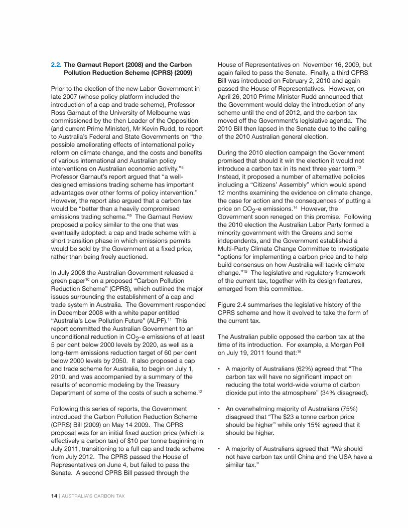
The presence of complementary measures such aswind and solar subsidies, the RET, and the CleanEnergy Finance Corporation means that achievingsuch equality of marginal costs is unlikely, if notimpossible. Consider, for example, the RET whichwas discussed in section 3.5.1 above. To understandthe costs of this scheme, consider Figure 4.2, whereabatement is plotted on the horizontal axis and can beproduced in two sectors, A and B. To reach theemissions target, QA+QB tonnes of abatement arerequired. Sector B is the renewable energy sector.Under an undistorted cap and trade scheme, permits
would be traded and the renewable energy sectorwould produce at the point where marginal abatementcosts are equalised. Under a mandatory renewableenergy target, however, sector B must produce QBtonnes of abatement. The marginal costs of achievingthe last unit of abatement in B exceed the marginalcosts of achieving the last unit in A. Hence themarginal costs of abatement are not equalised andabatement is not achieved at least cost. There is awelfare loss equal to the shaded triangle in thediagram. The only way such a scheme could achievea different outcome is if it either (i) achieved more thanQA+QB units of abatement, in which case the permitprice would be zero (and indeed there would be noneed for a cap and trade scheme) or (ii) if transactioncosts or some kind of market failure in the permitmarket prevented trade in permits from achieving theefficient outcome (in which case a cap and tradescheme may also not be desirable).25
4.2.2. The Effects of Household Assistance and Income Tax Changes
Another common argument for introducing a carbontax (or a cap and trade scheme in which permits areauctioned by the government) is that tax or permitrevenues can be used to reduce existing distortionarytaxes, such as personal income taxes. The “doubledividend hypothesis” refers to the idea that there may
Target for Sector B
MCA
MCA
MCB
QAOBOA QB
MCB
$/tonne ofabatement
$/tonne of abatement
FIGURE 4.2: THE COSTS OF A MANDATORYRENEWABLE ENERGY TARGET
26 | AUSTRALIA’S CARBON TAX
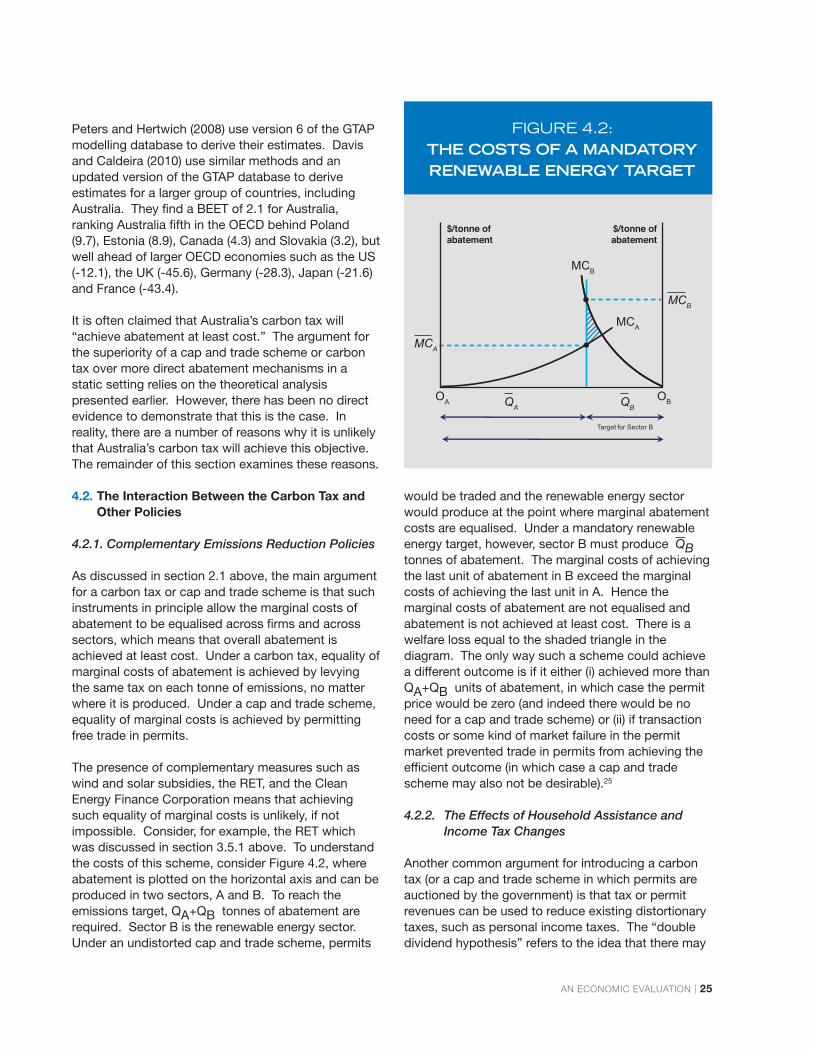
actually be two benefits from environmental taxation:the usual welfare gain that a Pigouvian tax bringsabout by reducing external costs, and an additionalgain which comes about from the reduction in thewelfare losses associated with existing taxes.However, it is unlikely that there is a double dividendin the case of Australia’s carbon tax for two reasons: a theoretical reason, and an empirical reason.
To understand why this is the case, we considerFigure 4.3, which models a simple situation in whichthere are two related markets, A and B, and assumedthat A and B are complements. There is an existingdistortionary tax of tAin market A, and consumption inmarket B causes a negative externality. Initialconsumption and production levels in each market areQ1
A and Q1B.
Now introduce a Pigouvian tax in market B. Since thegoods are complements, introducing this tax leads toa reduction in the consumption of both goods.Consumption and production fall to Q2
A and Q2B, and
the tax in B creates a benefit equal to the shaded areain B. However, it also exacerbates the negativewelfare effects of the existing tax in market A, leading
to a fall in welfare in that market equal to the shadedrectangle in market A. This is usually referred to in theliterature as the “tax interaction effect” and it canpartially (or even completely) offset any welfare gain inmarket B.
A reduction in the tax in market A will simply reducethis exacerbating effect, and so there is no sense inwhich there are “two” gains from introducing thePigouvian tax.
The analysis also shows that if there are existingdistortions in other markets and the goods arecomplements, then the optimal Pigouvian tax shouldbe set at a level that is lower than the marginalexternal harm. More formally, letting be thechange in welfare as a result of imposing thePigouvian tax tB, MSC be the marginal social cost ofactivity B, and letting be the initial price in B, wehave that the change in welfare in market B is:
BW
0Bp
PA0
QA2 QA
1
PA
PA
Market A
+ tA0
DA’DA
2 1
t
Begin at point “1” in
each panel. There is an
existing tax in market A,
and no tax in market B
But activity declines
in market A because
we lose some
revenue without reducing the tax. Overall welfare could even fall!
FIGURE 4.3: THE “TAX INTERACTION EFFECT”: THE WELFARE EFFECTS
OF A PIGOUVIAN TAX WHEN THERE IS A PRE-EXISTING DISTORTION IN A RELATED MARKET
PB0
QB1 QB
2 QB1
PB
PB
MSC
+ tB0 2
DB
1
Now levy a tax in market
B. We get the usual
welfare gain from a
Pigouvian tax in B.
Market A
( )0 BB B B
B
QW MSC p tt
= +
AN ECONOMIC EVALUATION | 27
where is the slope of the demand curve for good B.
On the other hand, the change in welfare in market Ais the change in revenue that occurs in that market,which is not offset by any gain in market A:
where is the shift in the demand for A when the
price of B rises.
The optimal (welfare maximising) Pigouvian tax is theone where the marginal welfare gain in market B justequals the marginal welfare loss in market A:
Rearranging this expression gives:
This expression tells us that:
• If there are no distortions in other markets, then theusual Pigouvian rule applies (set tax = marginalexternal harm);
• If there are existing distortions in other markets andthe goods are complements, then the optimalPigouvian tax should be set at a level that is lowerthan the marginal external harm; and
• If there are existing distortions in other markets andthe goods are substitutes, then the optimalPigouvian tax should be set at a level that is higherthan the marginal external harm.
For Australia’s carbon tax the case of complements isthe most empirically relevant one—the income tax isthe most significant pre-existing tax in the Australiantax system, and activities that the carbon tax effects(such as electricity, fuel, and so on) are
B
B
Qt
AA A
B
QW tt
=
A
B
Qt
( )0 B AABB
B B
Q QMSC p t tt t
+ =
0
External harm
Additional term
AA
BB B
B
B
Qttt MSC p Qt
=
complementary to labour. Hence the likely effect ofthe carbon tax is that it will decrease labour supply,exacerbating the distortionary effects of the existingincome tax system.
Whatever one thinks about the theory of the doubledividend hypothesis, actually implementing the idea inpractice requires marginal income tax rates to bereduced. As part of the carbon tax policy, theAustralian Government made a number of changes tothe personal income tax system to compensate forincreases in electricity prices and other householdcosts. However, as section 5.1 below shows, sincethe carbon tax will reduce GDP below the level itotherwise would have been in every year that it is inplace, full compensation for all taxpayers is notpossible. Hence average income tax rates remainedunchanged for a large number of taxpayers.
Table 4.1 below summarises the changes to statutoryand effective marginal tax rates for Australiantaxpayers as a result of the changes.26 As a result ofthe changes, effective marginal tax rates (EMTRs) fellfor those on incomes between $16,001 and $20,542(around 560,000 taxpayers), but increased for thoseon incomes between $20,543 and $30,000, as well asthose on incomes between $37,001 and $67,000 (atotal of around 2.2 million taxpayers). In other words,regardless of the textbook theory, in actual practicewhilst average income tax rates for many Australiansdeclined, more Australians saw their marginal incometax rates go up, rather than down, by a ratio of almost4-to-1.
As Williams (2011) explains, this increase in marginalrates was needed as part of the compensationpackage because of the revenue cost of theGovernment’s decision to increase the tax free
Since the efficiency costs of taxation
increase with the square of the tax rate,
these changes are likely to have led to
significant overall efficiency costs, even
taking into account the fact that
marginal rates were reduced for some
taxpayers.

28 | AUSTRALIA’S CARBON TAX
threshold, which reduced marginal rates for some lowincome earners. To claw back some of the foregonerevenue, marginal rates for those on higher incomeshad to be increased. Under the carbon tax policy,marginal income rates were increased for thosealready facing reasonably high tax rates. Since theefficiency costs of taxation increase with the square ofthe tax rate, these changes are likely to have led tosignificant overall efficiency costs, even taking intoaccount the fact that marginal rates were reduced forsome taxpayers.
The crucial point is that that this increase in effectivemarginal tax rates is the exact opposite of what thedouble dividend theory recommends. In other words,instead of using the tax system to offset some of thenegative welfare effects caused by the interactionbetween the carbon tax and the personal income taxsystem, the most likely effect of the AustralianGovernment’s income tax changes is that they haveactually made things worse and exacerbated thenegative effects of those interactions. Moreover, noneof these additional costs were taken into account inthe Government’s modelling of the effects of the tax.
TABLE 4.1: NEW STATUTORY INCOME TAX RATES, OLD EMTRS AND NEW EMTRS
APPROXIMATENEW CHANGE NUMBER OF
OLD STATUTORY NEW IN TAXPAYERSINCOME LEVEL EMTR RATE EMTR EMTR (MILLION)
$0-$16,000 0 0 0 NO CHANGE 0.28
$16,001-$18,201 0.15 0 0 FALL BY 0.15 0.28
$18,201- $20,542 0.15 0.19 0 FALL BY 0.15 0.28
$20,543-$30,000 0.15 0.19 0.19 RISE BY 0.04 1.38
$30,001- $37,000 0.19 0.19 0.19 NO CHANGE 1.19
$37,001- $67,001 0.34 0.325 0.34 NO CHANGE 3.58
$67,001- $80,000 0.3 0.325 0.325 RISE BY 0.025 0.83
$80,001- $180,000 0.37 0.37 0.37 NO CHANGE 1.19
>$180,001 0.45 0.45 0.45 NO CHANGE 0.18
SOURCE: WILLIAMS (2011).
4.3. International Linking and Restrictions on International Trade
4.3.1. The Gains from International Trade in Permits
The Australian Government has recently proposedmoving to a flexible price “cap and trade” scheme ayear earlier than originally intended, in 2014. Inprinciple, this may help to achieve abatement at lesscost. To see this, consider Figure 4.4 below, whichanalyses the economic effects of opening up theeconomy to trade in permits.
The figure plots the marginal private benefits andcosts of emissions. Before trade, the domestic tax is tD and domestic emissions are E. Now theeconomy is permitted to trade permits with the rest ofthe world, at the world price of tW < tD. The overallemissions target is still E, but at the world price of tWdomestic emissions now increase to ED. Domesticfirms purchase ED – E from the rest of the world.
Note that the external costs of emissions are irrelevanthere, due to the assumption that the target is fixedand so global emissions are the same before and afterthe economy opens up to trade. The economic effect

AN ECONOMIC EVALUATION | 29
is therefore similar to lowering an ordinary tax, takinginto account the fact that part of the revenue is nowtransferred to foreign firms. The domestic economygains the area a + b + c + d + e, which is the usualwelfare gain from lowering a tax. There is a transfer tothe rest of the world of b + d. Hence the overallwelfare effect is a gain of a + c + e. Note that bysimilar triangles, b + c = c + e, and so the welfare gain
is simply , which is
one half multiplied by the difference between thedomestic and foreign price, multiplied by the number offoreign permits purchased. Australia’s carbon tax in2014 is scheduled to be $25.40. In the Government’smodelling, there are 15 million tonnes of overseasabatement in 2014. At an EU price of $6, using theabove estimate we obtain a welfare gain from an earlymove to a link with the EU of $145.5 million, or less than0.01 per cent of Australia’s expected GDP in that year.
Any estimate of the gains from allowing internationaltrade in permits depends on the assumption that theEuropean Union keeps the same number of permits incirculation. If instead the EU meets the increase indemand for permits by increasing supply, then thewelfare gain for Australia would be much lower
because there would be less global abatement. If thatis the most likely scenario, the optimal policy is simplyto lower the carbon tax to the current EU price andnot bother linking. Domestic firms emit the sameamount as they would under the link to the EU, andglobal emissions would rise by the same amount asthey would if the EU issued more permits. But theAustralian government would earn additional revenue.
4.3.2. Constraints on Overseas Permit Purchases
Although there may be gains to Australia from linkingto the European scheme, there are a number ofreasons why such gains are likely to be smaller thanthose identified in the previous section. The primaryreason is that under the Government’s policy, liableentities must meet at least 50 per cent of their annualliability with domestic carbon units. This sectionexamines the effect of this constraint.
To understand the effects of this restriction, wesimplify Figure 4.4 in Figure 4.5 by assuming that themarginal private cost of emissions are zero. In thisdiagram, Dpermits is the Australian demand foremissions permits and is derived from the marginalcost of abatement curve. Throughout we assume thatthe world permit price is pW and that this is lower than
MPC+tW
a
bc
e
d
MPC
MB
MPC+tD
E EED
MC, P
FIGURE 4.4: INTERNATIONAL TRADE IN
EMISSIONS PERMITS
( )( )12 D D Wa b c E E t t+ + =
Price
Domestic Emissions
E1
pW
E0EW
Spermits
Dpermits
FIGURE 4.5: DOMESTIC EMISSIONS
AND ABATEMENT WITH FREETRADE IN PERMITS

30 | AUSTRALIA’S CARBON TAX
the domestic autarky price.
Suppose that Australia’s overall emissions target is E1.At a world price of pW, domestic firms want to emitEW i.e. they demand EW permits. The governmentissues E1 permits, and Australian firms pay overseasfirms to reduce their emissions at the world price ofpW. There is an income transfer from Australia tooverseas, equal to pW(EW- E1). Australia’s domesticabatement is E0-EW. Foreign abatement is EW- E1.The cost to Australia is the cost of abatement plus thecost of purchasing foreign permits.
Notice that in the above situation, more than 50 percent of aggregate emission liabilities are met bypurchasing foreign permits (EW is more than twiceE1). But this is not permitted under Australia’sscheme before 2020. Under the CEF policy, liableentities must meet at least 50 per cent of their annualliability with domestic carbon units. The aggregateeffect of this constraint is shown in Figure 4.6 below.In this scenario, the Australian government againissues E1 permits. But domestic firms are nowallowed to purchase at most EW’-E1 permits fromoverseas, with EW’ = 2E1. The remaining permitsmust be purchased domestically. This is akin toplacing a quota on foreign imports. The restrictionmeans that the supply curve is not flat at the worldprice, but takes the shape indicated in Figure 4.6.
Domestic firms now emit far less, 2E1 than they wouldhave if there was no restriction on the use of overseaspermits. To meet their obligations, they purchase E1at a world price of pW, and must purchase a furtherE1 from domestic sources. The marginal value of apermit at the point 2E1 is pDom. If domestic permitsare tradeable within Australia, then the price of thesepermits will be bid up until they reach pDom which,when the constraint on foreign permit purchasesbinds, must exceed the world price of pW.
Appendix B shows that the markup of the domesticpermit price over the world price will be equal to
, where is the elasticity
of domestic demand for permits evaluated at the levelof the target, EW is the level of domestic emissions atthe world price under free trade, and is the share ofannual liabilities that entities must meet with domesticcarbon units ( = 1/2 under the Australian Government’spolicy). The elasticity of demand for permits reflects
E
E
how rapidly marginal costs of abatement rise asabatement increases. The price of a domesticallyissued must therefore be equal to . Domesticabatement is now equal to E0-EW’> E0-EW. However,compared to a situation in which there are norestrictions on international permit purchases, there isan additional cost of “e” in Figure 4.6. The total costto Australia is e+f+g , which is the cost of abating E0-EW’) plus a payment of “d” to the rest of the world.Global emissions fall by E0-E1, which is identical tothe outcome that would be achieved in the absence ofrestrictions on international permit purchases. In otherwords, abatement in the Australian scheme is notachieved at least cost.
In fact, there may be an even less costly abatementoption. Consider what would happen if the AustralianGovernment directly purchased E0-E1 permits from therest of the world at the world price of pW, and simplywithdraws these permits from circulation (or destroyedthem). This has a cost to Australia of d+f+g+h, which issimply the income transfer to the rest of the world frombuying permits. Global emissions again fall by E0-E1,so there are no other costs or benefits to consider,apart from the costs of raising the revenue needed topurchase the required permits.
In theory, even if the taxes used to raise this revenuewere non-distortionary, this option would be morecostly than allowing domestic firms to reduce their
111 1 1W
EE
> 0<
Price
Domestic Emissions
E1 E’W(=2E1)
pDom
pW
E0EW
Dpermits
Spermits
hgfd
b
c
ae
FIGURE 4.6: DOMESTIC EMISSIONS AND
ABATEMENT UNDER AUSTRALIA’SCEF POLICY TO 2020

AN ECONOMIC EVALUATION | 31
emissions by E0-EW and then having them purchaseoverseas EW-E1 permits (the difference in costs of thetwo policies is the area “h” in the diagram). However,in practice that may not be the case. Indeed, usingthe Government’s estimate of GDP losses from thecurrent carbon tax over the period to 2020 (which areexplored in more detail in section 5.1 below), it ispossible to show that even if the marginal cost ofpublic funds27 is as high as 1.4, it would be cheaperfor Australia to abandon its carbon tax and insteaddirectly purchase emissions permits from the rest ofthe world and then withdrew those permits fromcirculation (i.e. destroy them).28 Since permits arewithdrawn from the EU market, global emissionswould fall by exactly the same amount as they wouldunder Australia’s current scheme - the only differenceis that Europe would be doing all of the abating ratherthan the effort being shared between Europe andAustralia. This analysis Australia’s carbon tax doesnot even pass a cost-effectiveness test, let alone amore stringent cost-benefit test.
4.4. Dynamic (In)efficiency
Another important reason why Australia’s carbon tax is
unlikely to achieve abatement at least cost is due tointertemporal considerations: if a carbon tax is set atan inappropriate level over time, then it can fail toachieve abatement at least cost in a dynamic setting.The Australian Government’s carbon tax modellinginitially assumed that the permit price would rise at thereal rate of interest, in accordance with a simpleversion of the Hotelling (1931) rule, which is derived inAppendix C. Intuitively, along an optimal abatementpath the present value of the marginal cost ofabatement should be constant, otherwise abatementcould be reallocated across time and a cost savingcould be made. Since competition in the permitmarket should force price down to marginal cost, thismeans that prices should grow at the real interest rate.
But despite earlier modelling which assumedotherwise, recently revised permit priceprojections in the Government Budget documents(shown in Figure 4.7) shows that Australia’s carbonprice is not expected to rise at the real rate of interest.Hence, according to the simple Hotelling rule, itcannot be the case that the carbon tax is minimisingthe cost of achieving a given fixed abatement target.In other words, there is no evidence that the carbontax will “achieve abatement at least cost” over time.
Car
bon
Pric
e (A
$ pe
r ton
ne C
O2-
e)
45
40
35
30
25
20
15
10
5
0
2012-2013 2013-2014 2014-2015 2015-2016 2016-2017 2017-2018 2018-2019 2019-2020
Revised Projected PricePath Initial Projected PricePath Current EU PriceMost Recent (2 August) Revised Projected Price Path
Year
FIGURE 4.7: CARBON PRICE PROJECTIONS, 2012-13 TO 2019-20
SOURCE: AUSTRALIAN GOVERNMENT BUDGET PAPERS PRE-ELECTION ECONOMIC AND FISCAL OUTLOOK; POINT CARBON.

32 | AUSTRALIA’S CARBON TAX
5. Economic and Fiscal Effects
Because the carbon tax has only been in place for just over 12 months, it is difficult to determine with any
great deal of precision the effect that it has had on macroeconomic outcomes such as GDP and
unemployment. Although there is mounting anecdotal evidence regarding the economic losses caused by
the tax (see section 5.3 below), and although the Australian Government has recently revised down its
official forecasts of economic growth over the near term, there is not enough data to undertake a formal
statistical analysis of the tax’s macroeconomic effects.
5.1. Gross Domestic Product (GDP) Losses
A number of earlier analyses of the tax suggest that itis likely to create significant economic costs. Forexample, McKibbin et al (2010) use the G-Cubedmodel to estimate the macroeconomic effects of thecommitments made under the Copenhagen Accord oflate 2009. The results, which are summarised in Table5.1 below, show that the annual costs to GDP forAustralia under the Copenhagen Accord will be 6.3per cent by 2020, which is much higher than the costsincurred by major economies included in the study,even though Australia’s Copenhagen commitment isrelatively modest by comparison.
The bulk of the costs of Australia’s carbon tax areexpected to be incurred over the medium to long termrather than in the short term. Modelling of theeconomic effects of the carbon tax by the Australian
TABLE 5.1: ESTIMATED GDP COSTS OF POLICY COMMITMENTS UNDER THE COPENHAGEN
COUNTRY/REGION POLICY COMMITMENT GDP LOSS IN 2020
UNITED STATES -15% ON 2000 LEVELS BY 2020 -2.7%JAPAN -37% ON 2000 LEVELS BY 2020 -5.1%AUSTRALIA -5% ON 2000 LEVELS BY 2020 -6.3%EUROPE -24% ON 2000 LEVELS BY 2020 -4.9%CHINA +350% ON 2000 LEVELS BY 2020 -3.7%OPEC +105% ON 2000 LEVELS BY 2020 -5.9%WORLD +70% ON 2001 LEVELS BY 2020 -3.2%
SOURCE: MCKIBBIN ET AL (2010)
Government suggests that the carbon tax willpermanently reduce GDP below what it otherwisewould have been in every year that it is in place, withthese costs growing over time. Although thereductions in annual growth appear to be relativelysmall when viewed in isolation, the value of the sum ofthese costs expressed in today’s dollars is likely to besignificant.
These Government modelling exercises, which havebeen examined in detail elsewhere,29 make a numberof unrealistic assumptions and as a result are likely tounderestimate the costs of Australia’s carbon tax. Themain reasons for this are as follows. First, thebaseline against which costs are measured assumethat the rest of the world takes similar action toAustralia. This is unrealistic for a number of reasons,

AN ECONOMIC EVALUATION | 33
not the least of which is that no other country currentlyhas an economy-wide carbon tax as high asAustralia’s. Second, the modelling also assumesaway a number of costs, such as those associatedwith the distortions caused by the income tax changesaccompanying the scheme (which are analysed insection 4.2.2 above), as well as the costs associatedwith carbon leakage, which are analysed in section 5.3below.
Nevertheless, the Australian Government’s modellingoutput can be used to indicate the rough magnitude ofthe GDP costs of introducing the carbon tax. Themodels estimate GDP over time with and without thecarbon tax, in various policy scenarios out to the year2050. Two scenarios are particularly relevant: thegovernment’s policy, and a “high price” scenario. Thegovernment policy scenario assumes a global targetof 550 CO2-e parts per million, with an Australianemission target of a 5 per cent cut on 2000 levels by
2020 and an 80 per cent cut by 2050. It also assumesa nominal domestic starting price of A$23 in 2012-13,rising at a real rate of 5 per cent per year, beforemoving to a flexible world price of $29 in 2015-16.The high price scenario, on the other hand, assumes aglobal target of 450 ppm, with an Australian emissiontarget of a 25 per cent cut on 2000 levels by 2020 andan 80 per cent cut by 2050. The starting price isassumed to be $30 in 2012-13, again rising at a realrate of 5 per cent, to be around $61 in 2015-16.
In each scenario GDP is estimated to be lower than itotherwise would have been. As is standard in cost-benefit analysis, the costs of the policy in eachscenario can be computed as the discounted presentvalue of the sum of the foregone GDP each year in thefuture.30 The results of these calculations are shown inFigure 5.1 for various discount rates, which are usedto convert the value of a dollar tomorrow to the valueof a dollar today so that consistent comparisons can
160%
140%
120%
100%
80%
60%
40%
20%
0%
Discount Rate
Pres
ent V
alue
of C
osts
as
a Sh
are
of C
urre
nt G
DP
0% 1% 2% 3% 4% 5% 6%
Government PolicyHigh Price Scenario
FIGURE 5.1: PRESENT VALUE OF PROJECTED ECONOMIC COSTS
OF AUSTRALIA’S CARBON TAX TO 2050
SOURCE: STRONG GROWTH, LOW POLLUTION; AUTHOR’S OWN CALCULATIONS.
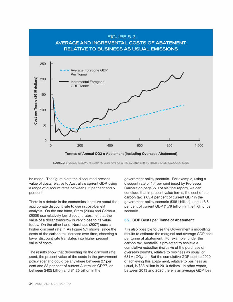
34 | AUSTRALIA’S CARBON TAX
be made. The figure plots the discounted presentvalue of costs relative to Australia’s current GDP, usinga range of discount rates between 0.5 per cent and 5per cent.
There is a debate in the economics literature about theappropriate discount rate to use in cost-benefitanalysis. On the one hand, Stern (2004) and Garnaut(2008) use relatively low discount rates, i.e. that thevalue of a dollar tomorrow is very close to its valuetoday. On the other hand, Nordhaus (2007) uses ahigher discount rate.31 As Figure 5.1 shows, since thecosts of the carbon tax increase over time, choosing alower discount rate translates into higher presentvalue of costs.
The results show that depending on the discount rateused, the present value of the costs in the governmentpolicy scenario could be anywhere between 27 percent and 83 per cent of current Australian GDP32, orbetween $405 billion and $1.25 trillion in the
government policy scenario. For example, using adiscount rate of 1.4 per cent (used by ProfessorGarnaut on page 270 of his final report), we canconclude that in present value terms, the cost of thecarbon tax is 65.4 per cent of current GDP in thegovernment policy scenario ($981 billion), and 118.5per cent of current GDP (1.78 trillion) in the high pricescenario.
5.2. GDP Costs per Tonne of Abatement
It is also possible to use the Government’s modellingresults to estimate the marginal and average GDP costper tonne of abatement. For example, under thecarbon tax, Australia is projected to achieve acumulative reduction (inclusive of the purchase ofoverseas permits, relative to business as usual) of681Mt CO2-e. But the cumulative GDP cost to 2020of achieving this abatement, relative to business asusual, is $33 billion in 2010 dollars. In other words,between 2013 and 2020 there is an average GDP loss
0 200 400 600 800 1,0000
50
100
150
200
250
Cos
t per
Ton
ne (2
010
dolla
rs)
Average Foregone GDPPer Tonne
Incremental ForegoneGDP Tonne
Tonnes of Annual CO2-e Abatement (Including Overseas Abatement)
FIGURE 5.2: AVERAGE AND INCREMENTAL COSTS OF ABATEMENT,
RELATIVE TO BUSINESS AS USUAL EMISSIONS
SOURCE: STRONG GROWTH, LOW POLLUTION, CHARTS 5.2 AND 5.13; AUTHOR’S OWN CALCULATIONS

AN ECONOMIC EVALUATION | 35
of $48 dollars for each tonne of abatement (more thanhalf of which is sourced from overseas), with costs ashigh as $142 per tonne in 2013. In other words, theeconomic cost of the carbon tax in terms of lost GDPper tonne far exceeds the headline carbon price.33
Figure 5.2 plots the average and incremental costs (interms of foregone GDP) of annual abatement, andshows that incremental costs rise rapidly asabatement rises.
It is important to note that the GDP costs of thecarbon tax examined in the previous section areinclusive of the compensation paid to households,which was examined in section 3.5.2. In other words,the compensation measures affect the distribution oflosses, but do not reduce the overall GDP losses (infact, as we argue above in section 4.2.2, thecompensation measures are likely to exacerbate theGDP losses).
As Appendix D shows, a pure matter of nationalincome accounting, the income that is foregone as aresult of the carbon tax must come broadly from eitherlabour income or business profits. Historically therelative shares of income flowing to labour and capitalin Australia have been around 60 per cent and 40 percent respectively. This suggests that the carbon taxwill lead to a larger proportional reduction in income tocapital than to labour income.
5.3. Business Costs, Profitability and Carbon Leakage
The main way in which business profits are likely to bedirectly affected under the carbon tax is via increasesin energy input costs. As Figure 5.3 shows, themanufacturing sector in Australia is the main user ofelectricity, followed by mining. The adverse effects ofthe carbon tax are therefore most likely to be directlyexperienced by electricity-intensive manufacturingactivities (such as refining, cement, aluminium, iron
50%
45%
40%
35%
30%
25%
20%
15%
10%
5%
0%
Sector
Shar
e of
Tot
al E
lect
ricity
Con
sum
ptio
n
FIGURE 5.3: SECTORAL SHARES OF TOTAL BUSINESS ELECTRICITY USE, 2011-12
SOURCE: ABS.

36 | AUSTRALIA’S CARBON TAX
and steel production) as well as certain types ofenergy-intensive mining activities (particularly coalmining, but also oil and gas mining).
Survey evidence suggests that many Australianbusinesses have been unable to pass on energy costincreases, which, according to the Australian IndustryGroup (AIG), have averaged 14.5 per cent forbusinesses as a result of the carbon tax. The AIG hasalso published the results of two business surveysdemonstrating how the carbon tax has affected inputcosts and profits.34 The survey found that of the threequarters of businesses that were able to estimate howmuch of their increased costs they were able to passon to their customers, 70 per cent said they had notbeen able to pass on any energy cost increases. Inother words, in these instances the economicincidence of the carbon tax fell on producers.
The most likely reason for the lack of pass-through ofthe carbon tax for these firms is that they are eitherproducing goods for export or are competing directlyagainst goods imported from overseas, and so face afixed world price for their output. In such cases thecarbon tax is likely to lead to carbon leakage ratherthan a reduction in global emissions.
Figure 5.4 provides a diagrammatic analysis of carbonleakage in a domestic import-competing industry. Inthe diagram, output and emissions are assumed to beproduced in constant proportions, and domestic firmsproduce in an industry in which there is a fixed worldprice of PW. At this price, domestic output andemissions are equal to E0 . Imports are initially E0 – E0 .
Now suppose that Australia introduces a carbon tax.Since domestic producers are price takers on theworld market, they cannot pass on any of the tax andso bear the entire economic incidence, receiving foreach unit of output. Domestic firms whose costsexceed this threshold are rendered unprofitable andare forced to exit the market.
Australia’s domestic output and emissions now fall toE1 . There is carbon leakage of E0 – E1 asthe rest of the world produces more output andemissions. Global emissions do not change, butAustralia’s imports now increase to E0 – E1 .Since there is no change in global emissions, there isno economic or environmental benefit and the tax issimply a tax on import competing firms. There is a
welfare loss equal to the shaded triangle in thediagram, with the incidence of the loss falling entirelyon domestic producers. The AIG survey evidencesummarised above suggests that the situationdescribed in Figure 5.4 is likely to be quite common. As discussed in section 3.5.2 above, under the carbontax’s “Jobs and Competitiveness Program”, certainemissions intensive trade exposed firms are issuedwith a declining amount of free permits. TheAustralian Government has argued that the “effective”carbon price for firms in emissions intensive tradeexposed industries is only $1.30, which is the permitprice multiplied by the share of permits that thesefirms receive for free. If true, this would mean thatfirms have little incentive to reduce emissions.However, this ignores the fact that firms makedecisions and respond to incentives at the margin.
Consider the following simple example of a profitmaximising firm whose output varies directly with itsemissions, so that its output (Y) is equal to itsemissions (E). The firm faces an output price of P andits cost function is C(E).
In the absence of a carbon tax, the firm’s output is:
Price
Output/Emissions
CarbonLeakage
CarbonTax
E0TotalE0
DomesticE1Domestic
S
D
PW
PW-t
FIGURE 5.4: CARBON LEAKAGE IN AN
IMPORT-COMPETING INDUSTRY
* arg max ( )E
E PE C E=

AN ECONOMIC EVALUATION | 37
If the firm faces a carbon tax of t, its output is:
Clearly E* < E**. In the presence of the carbon tax, thefirm will reduce its emissions and its profit will belower. Now suppose that the firm receives E freepermits. The firm’s output is now:
The firm reduces emissions by the same amount as itwould have if it did not receive free permits. The firmclearly prefers to receive free permits as this meansthat its profits are higher than they would be in theabsence of free permits. But at the margin the firmstill faces an “effective” carbon tax of t. The maineffect of allocating free permits to emissions intensive
trade exposed industries is that whilst marginal costsincrease by the amount of the tax, allocating freepermits means that average costs rise by less than thetax, and so average costs are lower than theyotherwise would be in the absence of free permits.Hence, if there are no barriers to exit, fewer firms mayexit the industry. However, as the number of freepermits is reduced over time, this effect will diminish.And irrespective of whether firms receive free permitsor not, the effect on global emissions is the same (i.e.there is no reduction).
5.4. Real Wages and Unemployment
None of the official Government reports discussed insection 2 above examined in detail the likely effects ofthe carbon tax on job losses and unemployment.Instead, the computable general equilibrium modelsthat were used in the modelling exercises typicallyassume that markets clear in the long run, so that any
** arg max ( )E
E PE C E tE=
( )***
**
arg max ( )
arg max ( )E
E
E PE C E t E E
PE C E tE tE E
=
= + =
0.00
-0.10
-0.20
-0.30
-0.40
-0.50
-0.60
-0.70
-0.80
-0.90
-1.002013 2014 2015 2016 2017 2018 2019 2020
Year
Leve
l Rel
ativ
e to
Bas
elin
e (p
er c
ent)
Real WagesGDP
FIGURE 5.5: ANNUAL REDUCTION IN REAL WAGES VERSUS ANNUAL REDUCTION IN GDP UNDER THE CARBON TAX, RELATIVE TO BASELINE, 2013-2020
SOURCE: SGLP

38 | AUSTRALIA’S CARBON TAX
labour market effects of the carbon tax mustultimately show up as reductions in real wages.Figure 5.5 shows that in percentage terms, even withcompensation in place, the Government expects thereduction in real wages relative to baseline to be muchlarger in relative terms than the overall reduction inGDP.
If labour market rigidities prevent real wages freelyadjusting in the manner suggested by Figure 5.5, thenthe introduction of the carbon tax means thatunemployment will be greater than would haveotherwise been the case. As Figure 5.6 shows, sinceJuly 2012 the number of unemployed workers inAustralia has risen by more than 10 per cent, from636,564 to 705,421, with the unemployment rate risingfrom 5.2 per cent to 5.7 per cent over the sameperiod.
There is mounting evidence that the carbon tax is
causing job losses in certain sectors, particularly inmanufacturing. Examples of job losses directlyattributable to the introduction of the carbon taxinclude the following:
• 22 May 2012: Norsk Hydro announced the closureof its aluminium smelter at Kurri Kurri in New SouthWales, resulting in the loss of jobs for around 350fulltime workers and 150 contractors. Thecompany had made at least one submission to theGovernment in 2009 highlighting that the carbontax “would put existing operation[s] at risk andrender an expansion unviable, stripping a potential$4 billion dollar investment and 3000 jobs from theAustralian economy.”
• 19 December 2012: Tamworth-based GrainProducts Australia announces the appointment ofvoluntary administrators amid concerns ofimpending insolvency, putting the future of 68
720
700
680
660
640
620
600
580
560
540
Carbon Tax Introduced
Pers
ons
Une
mpl
oyed
(Tho
usan
ds)
July2011
Sep2011
Nov2011
Jan2012
Mar2012
May2012
July2012
Sep2012
Nov2012
Jan2013
Mar2013
May2013
July2013
Month
FIGURE 5.6: UNEMPLOYMENT IN AUSTRALIA, JULY 2012 TO JULY 2013
SOURCE: ABS CAT. NO. 62XX, LABOUR FORCE, JULY 2013.

AN ECONOMIC EVALUATION | 39
employees at risk. The company’s directors cite a75 per cent rise in electricity costs over thepreceding three years as pivotal to the decision—and include reference to the carbon tax, saying thatthere has been no relief provided by the FederalGovernment and that “it is very hard formanufacturing in Australia to survive with these sortof increases.” Allied Mills ultimately agreed to buythe business in early 2013.
• 18 January 2013: Penrice Soda announces it willcease soda ash production at its Adelaide plant inJune, accounting for the loss of 60 jobs. Thecompany specifically cites the carbon tax, amongother factors, as having had a major bearing on itsdecision.
• 18 February 2013: Amcor announces that over 300jobs will be lost at its operations across Melbourneand Brisbane. The company stated that“significant cost increases including energy” wasone of the factors that “had a significant impact onour ability to remain competitive in the cartonboardmarket.”
• 11 March 2013: CSR announced a restructure ofits glass manufacturing business, Viridian, with theloss of 150 jobs overall at two sites—Ingleburn andWetherill Park. Rob Sindel, the Managing Director,confirmed that the carbon tax had added around$500,000 to the annual costs at its Ingleburnfacility.
As the carbon tax increases and further affectseconomic incentives, it should be expected to lead tofurther reductions in business profitability, job losses,and ultimately closures of certain businesses. Indeed,the whole purpose of the carbon tax is to reduce andeventually eliminate certain types of economicactivities, as well as the jobs that are created fromthese activities.
5.5. Consumer Prices
Part of the reduction in real wages relative to baseline(see Figure 5.5) brought about by the carbon taxoccurs as a result of a more rapid increase inconsumer prices than would otherwise be the case.The main direct effect on consumer prices has beenthrough electricity prices, as well as natural gasprices. These price increases are expected tocontinue over time as the carbon tax rises. Indeed,the Government’s modelling suggests that by 2050
the carbon tax will cause inflation adjusted wholesaleelectricity prices to be double what they otherwisewould be (see Table 5.2). This is expected to lead toan increase in retail electricity prices of around 32 percent above business-as-usual levels by 2050.35
The Australian Government stated that the carbon taxwould lead to “an average increase in householdelectricity prices of 10 per cent over the first five yearsof the scheme.” In most jurisdictions in Australia,retail electricity prices are subject to direct regulation.A number of estimates have indicated that the initialeffect of the tax on electricity prices have alreadyachieved the 10 per cent increase. The July 2012release of the TD Securities Melbourne InstituteMonthly Inflation Gauge stated that “due to theintroduction of the carbon tax from 1 July, the price ofelectricity rose by 14.9 per cent.”36 As Figure 5.7below shows, the increase in household electricityprices after the carbon tax was introduced was thehighest quarterly increase on record.
Table 5.3 shows that in the states of Queensland andNew South Wales, the carbon tax, together with other“green” electricity schemes (including the RETdiscussed in section 3.5 above) now account for up to19 per cent of a typical household electricity bill.
There has been some controversy in Australia over theissue of whether the carbon tax will reduce thequantity demanded of electricity when it isaccompanied by cash payments to households orpermanent tax cuts. As Appendix E shows, standardconsumer theory can be used to analyse this
TABLE 5.2: ESTIMATED EFFECT OF THE
CARBON TAX ON WHOLESALEELECTRICITY PRICES TO 2050
YEAR 2013 2030 2040 2050
ESTIMATED %INCREASE ABOVE 43.18 61.76 90.54 104.05BUSINESS AS USUAL
SOURCE: STRONG GROWTH, LOW POLLUTION, CHART 5.27.

40 | AUSTRALIA’S CARBON TAX
question. The quantity of electricity demanded by anindividual can actually increase under the carbon tax ifthere is enough overcompensation,37 when thepercentage increase in disposable income as a resultof cash payments and other tax changes exceeds thedifference between the expenditure share of the goodand the price change multiplied by the ratio of thecompensated elasticity to the income elasticity.
The main implication is that it is likely that the quantityof electricity demanded will fall in response to thecarbon tax—but for some individuals the fall is likely tobe less than would have occurred in the absence ofcompensation.
Whilst the direct effect of the carbon tax on electricityprices has been reasonably well documented, there
has been no attempt by Government agencies todirectly estimate the actual effect of the tax on theoverall price level since it has been in place. Beforethe tax was introduced, the Government estimatedthat the Consumer Price Index (CPI) would rise by 0.7per cent more than it would have in the absence of thetax. However, the accuracy of this forecast has notbeen verified ex-post. Indeed, on July 25, 2012 theAustralian Bureau of Statistics’ (ABS) Consumer PriceIndex release stated that:
“The ABS will not be able to quantify the impact ofcarbon pricing, compensation or other governmentincentives and will not be producing estimates ofprice change exclusive of the carbon price ormeasuring the impact of the carbon price.”
Sep1980
Sep1982
Sep1984
Sep1986
Sep1988
Sep1990
Sep1992
Sep1994
Sep1996
Quarter
Sep1998
Sep2000
Sep2002
Sep2004
Sep2006
Sep2008
Sep2010
Sep2012
Carbon TaxIntroduced
0
0.5
1
1.5
2
2.5
Inde
x of
Hou
seho
le E
lect
ricity
Pric
es (S
ep 1
980=
1)
FIGURE 5.7: INFLATION-ADJUSTED HOUSEHOLD ELECTRICITY PRICES,
1980 TO 2013
SOURCE: AUSTRALIAN BUREAU OF STATISTICS, CAT. NO. 6401.0 CONSUMER PRICE INDEX, AUSTRALIA, TABLE 7; AUTHOR’S CALCULATIONS.

AN ECONOMIC EVALUATION | 41
The ABS also stated that:
“The ABS is unable to measure the impact of thecarbon price. It is therefore not known if thechanges in prices are a one-off impact orcontinuing into future quarters.”
In February 2009 the Reserve Bank of Australia said inrelation to the carbon tax that it “should be able tolook through the initial increase in inflation” whenassessing the consequences for monetary policy.However, since no official estimates of the actualeffects of the carbon tax on the Consumer Price Indexexist, it is unclear how this has been achieved. Whilstinflation in Australia has remained low, the preciseeffect of the carbon tax on the overall price levelremains unknown.
5.6. Fiscal Effects
After several years of budget surpluses between 1996and 2007, Australia’s Federal Government has runbudget deficits in each year since 2008, with netgovernment debt increasing from negative $45 billion toan expected $219 billion in 2015-16. An importantfeature of Australia’s fiscal situation in recent years is thatrevenues from individual taxes, as well as aggregaterevenues, have become more difficult to predict.
The carbon tax will have two broad effects on theGovernment’s budgetary position. On the one hand,the carbon tax is expected to directly raise a
substantial amount of revenue.40 In addition, theexcise rebate reduction—which is an equivalentcarbon price applying to business transport emissionsfrom liquid fuels (rail and shipping) and non-transportemissions from businesses using liquid fuels—will alsoresult in higher revenue.
On the other side of the budget, the carbon tax policyinvolves additional spending and/or tax reductions tocompensate some households, selected tradeexposed industries, and billions of dollars in otheroutlays.41 The carbon tax may also lead to a reductionin company tax revenue and personal income taxrevenues below what they otherwise would havebeen, although this has not been quantified.
Despite raising a large amount of revenue, Figure 5.8shows, in its initial years the carbon tax was expectedto worsen Australia’s budget position, leading tohigher deficits and higher public debt than wouldotherwise have been the case. The cumulative fiscalshortfall was initially expected to be $4.4 billion overthe period 2011-12 to 2014-15.
TABLE 5.3:ESTIMATED CONTRIBUTION OF THE
INTRODUCTION OF THE CARBON TAX AND OTHER GREEN SCHEMES TO A TYPICAL ANNUAL HOUSEHOLD
ELECTRICITY BILL, QLD AND NSW
QLD (2012-13) NSW (2013-14)
RENEWABLE ENERGY TARGET $102 $107
SOLAR BONUS SCHEME/OTHER SCHEMES $67 $53
CARBON TAX $190 $172
TYPICAL HOUSEHOLD BILL $1900 $2073
GREEN SCHEMES/TOTAL 19 PER CENT 16 PER CENT
SOURCE: QLD - MINISTER FOR ENERGY AND WATER SUPPLY, MEDIA STATEMENT, 30 MAY 2013.38
NSW – INDEPENDENT PRICING AND REGULATORY TRIBUNAL, REVIEW OF REGULATED ELECTRICITY PRICES 2013-16, FINAL REPORT.39
There is mounting evidence that the
carbon tax is causing job losses in
certain sectors, particularly in
manufacturing.

42 | AUSTRALIA’S CARBON TAX
Figure 5.8 illustrates one of the most significantproblems with the design of the overall carbon taxpolicy: the mismatch between the tax’s revenueinflows and the outflows from compensationmeasures. The changes to the personal income taxsystem were introduced well before the tax came intoeffect, and were effectively “locked in” (althoughadditional tax cuts that were originally promised tocome into effect in 2015-16 have since beenrescinded). This means that a significant portion ofthe compensation for the carbon tax was based onassumptions about the uncertain future path of carbonprices. In practice, when the floating price periodbegins, the carbon tax rate will fluctuate substantially,as will the revenues that the tax raises.
In other words, the carbon tax has introduced anadditional source of uncertainty into the Government’sbudget projections: carbon tax revenues are likely tobe relatively volatile, whilst much of the outlays andcompensating tax reductions are difficult to change.As Figure 5.9 shows, the most recent estimates ofcarbon tax revenue for 2014-15 and 2015-16 are nowless than half the original revenue estimates. Shouldthe most recent projections eventuate, there will be agrowing negative gap between the revenuesgenerated by the tax and the increases in governmentspending that have accompanied the scheme.42
In the floating period, changes in the carbon tax willaffect both the revenue and expenditure side of theFederal Government’s Budget. The Departments ofTreasury and Finance have recently estimated a
35,000
30,000
25,000
20,000
15,000
10,000
5,000
0
-5,000
-10,000
$24,470 million
$3,300 million -$15,356 million
-$9,222 million
$-3,192 million
Revenue frompermit sales
Revenue from othermeasures
and fuel taxcredit
HouseholdAssistance
FreePermits
Overall Fiscal Impact-4,380 million
OtherPrograms
$ m
illio
n
Measure
FIGURE 5.8: EXPECTED CUMULATIVE FISCAL IMPACT OF THE CARBON TAX
AND ASSOCIATED POLICIES, 2011-12 TO 2014-15
SOURCE: SECURING A CLEAN ENERGY FUTURE: THE AUSTRALIAN GOVERNMENT’S CLIMATE CHANGE PLAN,TABLE 1 PAGE 131, AND TABLE 1 PAGE 135.

AN ECONOMIC EVALUATION | 43
simple rough “rule of thumb”, which states that a $1change in the carbon tax in any given year would be achange in the Budget bottom line (in underlying cashterms) balance of around $160 million in 2014-15 oraround $220 million in either 2015-16 or 2016-17.43
5.7. Effect on CO2-e Emissions
5.7.1. Overall Emissions
It is important to note that whilst emissions in theelectricity sector were expected to fall almostimmediately as a result of the carbon tax,44 thepurpose of the tax is not to reduce Australia’s overallemissions below current levels in the short to mediumterm. The main expected effect of the tax ondomestic emissions levels is to reduce them below
projected “business as usual” levels, rather thanreducing the absolute level of emissions. Indeed, theGovernment’s own modelling suggests that under thecarbon tax Australia’s domestic emissions are notexpected to stop increasing until 2027, and are notexpected to fall below current levels until 2043 (seeFigure 5.10).
5.7.2. Electricity Sector Emissions
As Figure 5.11 shows, electricity emissions in Australiahave been falling since 2008-09, due to both supplyside factors (mainly through the RET) and demandside factors (primarily increases in regulated retailprices for reasons unrelated to the carbon tax).Electricity demand fell by 5.5 per cent in response to a35 per cent real increase in retail electricity prices over
8,000
7,000
6,000
5,000
4,000
3,000
2,000
1,000
02012-13 2013-15 2014-15 2015-16
$ m
illio
n
Federal Budget 2012-13
Federal Budget 2013-14
MYEFO 2012-132nd August 2013 Economic Statement
FIGURE 5.9: INITIAL ESTIMATES AND REVISIONS OF CARBON TAX REVENUE,
2012-13 TO 2016-17
SOURCE: AUSTRALIAN GOVERNMENT BUDGET PAPERS AND STATEMENTS, VARIOUS ISSUES.

44 | AUSTRALIA’S CARBON TAX
the period, with electricity emissions falling by nearly12 per cent.
Despite this fall in emissions, data from the AustralianGovernment indicates that brown and black coal stillaccounted for around 79 per cent of total electricityproduction in Australia’s National Electricity Market inthe year to December 2011, before the carbon tax wasintroduced.
Standard producer theory can be used to examine thetheoretical long run change in the mix of electricityproduction in response to an increase in input pricesbrought about by a carbon tax. The total responsedepends on a substitution or supply-side effect, andan output or demand-side effect. To see this,
suppose that as a result of the carbon tax beingintroduced, the after tax price of an electricity input(for example, black coal), labelled j, rises. Then thechange in generators’ demand for alternative sourcesof energy is given by:45
where is the elasticity of demand for input i (analternative source of energy, for example, such aswind or solar) in response to an increase in wj, theafter tax price of the input subject to the carbon tax;
is the share of input j in total electricity productioncosts, is the (Allen) partial elasticity of substitutionbetween inputs i and j,46 < 0 is the consumer price
js
20132015
20172019
2021
Domestic emissions areprojected to peak in 2027
20232025
20272029
20312033
20352037
20392041
20432045
20472049
480
500
520
540
560
580
600
620
640
660
CO2-
e Em
issi
ons (
Mt)
Domestic emissions areprojected to fall below current
levels in 2043
Year
FIGURE 5.10: GOVERNMENT PROJECTIONS OF AUSTRALIA'S DOMESTIC
CO2-E EMISSIONS UNDER THE CARBON TAX, 2013-2050
SOURCE: STRONG GROWTH LOW POLLUTION, CHART 5.2
1
1
1/ (1 )1/ (1 )
ijijijjj
ms sm
+= =+
ij
ij

AN ECONOMIC EVALUATION | 45
elasticity of demand, and is a measure of returns toscale in electricity production. The parameter
is the markup of retail electricityprices over marginal costs. If the production functionfor electricity exhibits constant returns to scale thenwe have:
These expressions demonstrate that the theoreticaleffect of the carbon tax on the quantity supplied ofalternative sources of electricity inputs consists of twoconceptually separate effects. The first effect is that,holding output constant, the tax may cause electricityproducers to switch to alternatives, depending on theelasticity of substitution. The second effect is ademand-side effect: the tax will reduce consumerdemand for electricity as it becomes more expensive,and the quantity demanded falls. The latter twovariables are likely to be relatively small (particularly inthe medium term, as substitution possibilities are
limited on both the supply and demand sides), meaningthat a relatively large carbon tax would be needed toreduce emissions in the short to medium term.
The Australian Government expects the electricitysector to be the most significant source of domesticemission reductions under the carbon tax, deliveringover 40 per cent of total domestic abatement over theperiod to 2020. This equates to a 3.4 per centreduction in the absolute level of emissions generatedby the electricity sector on 2012 levels. Under thecarbon tax, around half of total electricity sectorabatement is expected to come from the demand sideof the electricity market.47
Given that inflation adjusted electricity prices rose by35 per cent in the four years prior to the carbon taxand that this produced a 5.5 per cent reduction inelectricity demand over the period, the extent to whichthe carbon tax will contribute to the expected demand
Dec02
Jun03
Dec03
Jun04
Dec04
Jun05
Dec05
Jun06
Dec06
Jun07
Dec07
Quarter
Jun08
Dec08
Jun09
Dec09
Jun10
Dec10
Jun11
Dec11
Jun12
Dec12
CO
2-e E
mis
sion
s (M
t)
44
46
48
50
52
54
56
Seasonally Adjusted
Trend
FIGURE 5.11: AUSTRALIA’S ELECTRICITY CO2-E EMISSIONS, 2002-2012
SOURCE: AUSTRALIAN GOVERNMENT, QUARTERLY UPDATE OF AUSTRALIA'S NATIONAL GREENHOUSE GAS INVENTORY, DECEMBER 2012
( )i j ij js= +
11/ (1 ) 1m = + >

46 | AUSTRALIA’S CARBON TAX
side effect remains unclear—particularly if the tax fallsto the current EU price of around $6, as theGovernment expects it will in 2014. The effect of thecarbon tax on actual electricity emissions has beendifficult to ascertain. In its recent report on the effectof the carbon tax on the National Electricity Market(NEM), the Australian Energy Market Operator (AEMO)found that “CO2-e intensity was largely unaffected inthe first quarter of carbon pricing.”48 It also found that
“The mix of fuels used to generate electricity in theNEM has changed since the start of carbon pricing,but not always to the extent anticipated before 1July 2012. Coal-fired generation reduced, but themajority of change to brown coal generationoccurred due to flooding in the Yallourn open-cutmine before the introduction of carbon pricing.”
As Figure 5.12 shows, official government data showsthat Australia’s overall emissions have risen relativelyrapidly since the introduction of the carbon tax. Giventhat a fall in the absolute level of Australia’s domesticemissions is not expected for another 15 years underthe carbon tax, this is not surprising.
Dec2002
Jun2003
Dec2003
Jun2004
Dec2004
Jun2005
Dec2005
Jun2006
Dec2006
Jun2007
Dec2007
Quarter
Jun2008
Dec2008
Jun2009
Dec2009
Jun2010
Dec2010
Jun2011
Dec2011
Jun2012
Dec2012
0
125
130
135
140
145
Emissions since the introduction of the carbon tax
Qua
rter
ly C
O2-
e Em
issi
ons
(Mt)
FIGURE 5.12: AUSTRALIA’S TOTAL CO2-E EMISSIONS, SEASONALLY ADJUSTED
WEATHER NORMALISED, 2002-2013
SOURCE: AUSTRALIAN GOVERNMENT, QUARTERLY UPDATE OF AUSTRALIA'S NATIONAL GREENHOUSE GAS INVENTORY, DECEMBER 2012.49

AN ECONOMIC EVALUATION | 47
6. Conclusions: Policy Lessons from the Australian Experience
There are a number of important lessons that policymakers around the world can draw from Australia’s
carbon tax experience.
Lesson 1: In Assessing the Case for a Carbon Tax or Cap and Trade Scheme, Estimate the
Incremental Net Benefits of All Feasible Policy Options, Rather than the Possible
Costs of Climate Change
The role of climate change policy is not to assess the possible damage of climate change, but ratherto focus on the incremental net benefits of possible policy options. This is the domain of cost-benefitanalysis. Whilst a number of Australian reports examined the expected economic costs of the carbontax, there was never a full cost-benefit analysis of various options. In particular, there was never anassessment of the incremental net benefits to Australia of limiting emissions, versus other measuressuch as adaptation. The debate has been framed as limiting emissions on the one hand, versus doingnothing on the other.
The most important feature of climate change policy isthat any policy (even the policy of doing nothing) ismade under conditions of uncertainty and ignorance.Policymakers are unlikely to know what individual oraggregate abatement costs look like—either in total orat the margin—or indeed what the aggregate marginalbenefits of abatement look like, either for individualcountries or the world as a whole. And no matterwhat targets and timetables are announced by variouscountries, policymakers cannot know for sure todaywhat other countries will actually do in the future – asopposed to what they say they will do.
Climate science may give us some idea of thepossible effects of abatement (i.e. the avoided effectsof climate change), but climate science cannot tell uswhat the economic difference is between (say)reducing emissions by 60 per cent of 2000 levels by2040, or 80 per cent of 2000 levels by 2050. Thesequestions are impossible to answer without aneconomic framework. But these and similar questionsabout economic tradeoffs are obviously very importantfor policymakers.
When policymakers are uncertain or ignorant aboutregarding the position of marginal costs and benefitcurves, no climate change policy will be perfect—all
policies will create welfare losses, unless they justhappen by chance to be right. Contrary to theAustralian Government’s approach, the relevantquestion for responsible economic policymakers is notwhether one policy instrument (such as a tax or a capand trade scheme) is more likely to achieve anenvironmental target, but which instrument creates thelowest welfare loss on average (i.e. the lowestexpected deadweight loss), taking into account allcosts and benefits. This involves careful,comprehensive and realistic assessment of:
(i) The likely effects of policy changes on economicand environmental variables (such as the globaltemperature), relative to a realistic baseline;
(ii) The likelihood of other countries undertakingsimilar policies, taking into account the very realrisk that countries may commit to take action butlater renege on such commitments;
(iii) The incremental costs and benefits of all feasiblepolicy changes, including adaptation;
(iv) The nature and magnitude of the uncertaintysurrounding estimates of costs and benefits ofvarious policies.

48 | AUSTRALIA’S CARBON TAX
Unfortunately, despite the Australian Governmentissuing a number of reports on climate change policy,such an analysis has never been undertaken. Thereports focused on estimates of the costs of climatechange rather than the costs that would actually beavoided by policies that were being considered.
Lesson 2: Do Not Ignore the Effects and Costs of “Complementary” Policies, Which Are Likely to Result in Efficiency Losses Rather than Efficiency Gains, Compounding any Negative Effects of a Carbon Tax or Cap and Trade Scheme
Proponents of carbon taxes argue that “marketmechanisms” - cap and trade schemes and carbontaxes - are superior to direct command and controlalternatives. The conventional economic argument isthat introducing a price will allow other more costlyschemes (such as renewable energy targets, greensubsidies, efficiency standards and other forms ofregulation) to be abolished. Proponents argue thatsince a cap and trade scheme achieves abatement atleast cost, once the emissions or abatement target isfixed under a cap and trade scheme, the existingschemes will not create further emissions reductions(unless the “cap” is in addition to emissionsreductions achieved by these other schemes).
Although this is intuitively appealing, there have beena number of practical difficulties with this argument inAustralia’s case. Firstly, the Australian Governmenthas never actually demonstrated that “marketmechanisms” are superior to non-market alternatives.Furthermore, many features of the policies thataccompany Australia’s carbon tax bear a strongresemblance to command and control policies. Mostnotably, Australia’s Renewable Energy Target hasremained in place. In addition, the carbon taxlegislation introduced new forms of intervention,including the Clean Energy Finance Corporation. In
practice, complementary policies have remained inAustralia, even after the carbon tax was put in place.Hence any hypothetical efficiency gains that may haveoccurred as a result of eliminating other programshave not materialised. The failure to remove existing“complementary” policies and the introduction of newinstruments has also weakened the intellectual casefor adopting so-called “market mechanisms.”
Lesson 3: Cumulative Economic Costs are Likely to be Substantial Over the Long Term, with Lower Discount Rates Resulting in Higher Cumulative Costs in Present Value Terms
The analysis in section 5 shows that although annualcosts appear to be small (a fact which proponents liketo emphasise), the cumulative costs of Australia’scarbon tax are likely to be high. The results show thatdepending on the discount rate used, the presentvalue of the costs in the government policy scenariocould be as high as 83 per cent of current AustralianGDP. These costs must ultimately manifestthemselves as lower incomes to capital or labour.
Lesson 4: Fiscal Impacts are Likely to be Uncertain, with both Carbon Taxes and Cap and Trade Schemes Adding to any Existing Revenue Volatility
By deliberate design, the Australian Government’shousehold compensation package was locked in overtime and was based on assumptions about the path ofcarbon prices and emissions. In practice, emissionsare uncertain, and after 2015-16 the price willfluctuate. This means that there is likely to be asizeable fiscal gap between the revenues generatedby the tax on the one hand, and the increases ingovernment spending and tax cuts that accompaniedthe scheme on the other. In other words, the carbontax has actually worsened Australia’s budget bottomline, leading to higher deficits and higher public debtthan would otherwise have been the case. Thecarbon tax has introduced an additional source ofvolatility into the Australian Government’s taxrevenues.
The most important feature of
climate change policy is that any policy
(even the policy of doing nothing) is
made under conditions of uncertainty
and ignorance.

AN ECONOMIC EVALUATION | 49
Lesson 5: Carefully Assess the Possibility and Costs of Carbon Leakage
The effect of a carbon tax on emissions-intensive,trade-exposed industries is similar to a tax on exportsor a tax on import-competing industries. Domesticemissions in these industries may fall after a carbontax is imposed, but that cannot be counted as anenvironmental gain if the ultimate effect is thatemissions simply rise overseas. The net effect is apure deadweight cost to the economy.
Lesson 6: The Double Dividend is Elusive
Carbon tax proponents often claim that carbon taxrevenue can be “recycled” and used to reducemarginal income tax rates, thus providing a “doubledividend.” This is a dubious proposition in theory dueto the interaction between the carbon tax and existingtaxes. These interactions were never taken intoaccount in the Government’s modelling.
In Australia’s case, as part of the compensationpackage for the carbon tax, the AustralianGovernment lowered some average income tax ratesbut actually increased marginal tax rates for around 2million taxpayers. Instead of mitigating the adverseeffects of the carbon tax on the labour market, thesechanges to the personal tax system have likelyexacerbated those effects. The increase in marginaltax rates is exactly the opposite policy of what aGovernment would do if it was trying to capture a“double dividend” from environmental taxation.
Lesson 7: Establishing a Robust, Sustainable and Credible Carbon Tax is Politically Difficult. Policy Uncertainty and Time Inconsistency are the Norm Rather thanthe Exception
The politics of carbon tax interacts with the economiceffects in important ways. During the 2010 electioncampaign the Australian Government promised thatshould it win the election it would not introduce acarbon tax in its next three year term. Despite thiscommitment, the Government introduced the tax afterthe election, even though the Australian publicopposed the policy, and political support for it hasbeen weak. Major changes were made to the taxalmost as soon as it took effect, and the Governmenthas recently announced further major changes. As aresult, there is a great deal of uncertainty surroundingthe future status and design features of the tax. Oneof the theoretical justifications for introducing a carbontax is that it provides a credible price signal andencourages future investment in alternative energysources. With so much uncertainty surroundingcurrent arrangements in Australia, it is doubtfulwhether the current price signal is very strong.
Major changes were made to the tax
almost as soon as it took effect, and the
Government has recently announced
further major changes. As a result,
there is a great deal of uncertainty
surrounding the future status and
design features of the tax.

50 | AUSTRALIA’S CARBON TAX
Ergas, H and Robson, A (2012) “Modelling as Agit-prop: The Treasury’s role in Australia’s carbon tax debate”, Agenda, vol. 19, no. 2,pp. 9-21.
Cahuc, P. and Zylberberg, A. (2001) Labor Economics, Cambridge, MA: MIT Press. Garnaut, R. (2008) Climate Change Review Draft Report, June. Harrison, M. (2010) Valuing the Future: The Social Discount Rate in Cost Benefit Analysis, Visiting Researcher Paper, Productivity
Commission, April. McKibbin. W. and P. Wilcoxen (2002) Climate Change Policy After Kyoto: Blueprint for a Realistic Approach, Washington DC:
Brookings. McKibbin, W. et al (2011) “Comparing Climate Commitments: A Model-Based Analysis of the Copenhagen Accord,” Climate Change
Economics, 2(2): 79-103. Nordhaus, W. (2007) “To Tax or Not to Tax: Alternative Approaches to Slowing Global Warming” Review of Environmental Economics
and Policy, 1(1): 26-44. Peters, G. and Hertwich, E. (2008). “CO2 Embodied in International Trade with Implications for Global Climate Policy.” Environmental
Science and Technology, 42(5): 1401–1407.Robson, A. (2007) “The Prime Ministerial Task Group’s Report on Emissions Trading: A Solution in Search of a Problem”, Agenda 14(3):
19–25.Robson, A. (2009) “ETS Forum: Why No Cost–Benefit Analysis?” Quadrant Online, 8 August, at:
http://www.quadrant.org.au/blogs/doomed-planet/2009/08/alex-robsonRobson, A. (2010), “What does the Government’s CPRS Modeling Tell Us?”, in A Moran (ed.), Climate Change: The Facts, Institute for
Public Affairs, Melbourne.Williams, M. (2011) “Why Increasing the Tax-Free Threshold is a Bad Idea”, IPA Review, 63(3): 27-28.
References

AN ECONOMIC EVALUATION | 51
Appendices
Appendix A: The Clean Energy Future Legislation
The 18 pieces of legislation are as follows:
The Carbon Pricing Architecture
• Clean Energy Act 2011
• Clean Energy (Consequential Amendments) Act 2011
Establishment of Statutory Bodies
• Climate Change Authority Act 2011
• Clean Energy Regulator Act 2011
Household Assistance Measures
• Clean Energy (Household Assistance Amendments) Act 2011
• Clean Energy (Tax Laws Amendments) Act 2011
• Clean Energy (Income Tax Rates Amendments) Act 2011
Changes to the Fuel Tax Rebate
• Clean Energy (Fuel Tax Legislation Amendment) Act 2011
• Clean Energy (Excise Tariff Legislation Amendment) Act 2011
• Clean Energy (Customs Tariff Amendment) Act 2011
Charges Associated with the Carbon Pricing Mechanism
• Clean Energy (Charges—Excise) Act 2011
• Clean Energy (Charges—Customs) Act 2011
• Clean Energy (Unit Issue Charge—Auctions) Act 2011
• Clean Energy (Unit Issue Charge—Fixed Charge) Act 2011
• Clean Energy (Unit Shortfall Charge—General) Act 2011
• Clean Energy (International Unit Surrender Charge) Act 2011
• Ozone Protection and Synthetic Greenhouse Gas (Manufacture Levy) Amendment Act 2011
• Ozone Protection and Synthetic Greenhouse Gas (Import Levy) Amendment Act 2011.
Further details of the Acts can be found on pages 23-25 of the Explanatory Memorandum50 to the legislation.

52 | AUSTRALIA’S CARBON TAX
Appendix B: The Price of Domestic Permits with Restrictions on Purchases of Overseas Permits
Section 4.3.2 argued that the price of domestic permits is likely to exceed the overseas price, and provided anexpression for the price markup. This section demonstrates how that expression is derived.
Consider the figure above, which is identical to Figure 4.6 in the main text. In the figure, the government issuesE1 domestic permits, but allows Between PDom and PW, the elasticity of the demand curve is approximatelyequal to:
So that:
Manipulating this equation gives:
Now is the share of annual liabilities that entities must meet with domestic carbon units.Hence the markup is:
This is the expression in the main text.
Price
Domestic Emissions
E1 E’W(=2E1)
pDom
pW
E0EW
Dpermits
Spermits
hgfd
b
c
ae
'W W
W
Dom W
W
E EE
p pp
=
'Dom W W W
W W
p p E Ep E
=
'11Dom W
W W
p Ep E
= +
'1 WE E= , where
111 1 1Dom
WW
p Ep E
= >

AN ECONOMIC EVALUATION | 53
Appendix C: The Hotelling Rule and Least Cost Abatement
This appendix derives the simple Hotelling rule for abatement at minimum cost across time. Suppose that aneconomy wishes to reduce its annual emissions from E0 today to E1 < E0 in the future. This can be achievedthrough costly abatement. Suppose further that the total cost of undertaking actions that permanently achieve
abatement of at in period t is c(at). To achieve the emissions target, total abatement must satisfy .
Suppose that the policy objective is to abate at least cost; that is, to minimise the present value of the total costs
of achieving this abatement, .
Let C(Et) be the present value of the cost beginning at time t of reaching the target ET, given that currentemissions are Et. The Bellman equation is:
subject to . The first order condition for this problem is:
and the envelope theorem gives:
So:
This states that to minimise the present value of the costs of achieving a given emissions reduction target, themarginal cost of abatement should grow at the rate of interest.
00
T
T tt
E E a=
=
( )( )0 1
Ttt
t
c ar= +
( ) 1 1( )( ) min1t
t tt t ta
C EC E c ar
+ += ++
( ) 1 1'( )'1t t
tC Ec a
r+ +=
+
1 1'( )'( )1t t
t tC EC E
r+ +=
+
( ) ( )11 1 ''( )'( )1 1
tt tt t t
c aC Ea C Er r
++ += = =+ +
1t t tE E a+ =

54 | AUSTRALIA’S CARBON TAX
Appendix D: Accounting for Reductions in GDP Relative to Baseline
This Appendix illustrates how the reduction in GDP relative to baseline will fall on labour income and capitalincome, as discussed in section xx in the text. Let Y(t) denote the level of GDP at time t. Then the incomedefinition of GDP states that:
where r(t) is the gross rate of return to the capital stock K(t), w(t) is the real wage rate, and L(t) is the level ofemployment in time t. Taking the derivative with respect to time and dividing by Y(t) on both sides yields:
where sK is the income share of capital and a dot over a variable indicates a derivative with respect to time. Thisexpression states that the percentage reduction in GDP relative to business as usual at time t is equal to theweighted average of the percentage reduction in returns to capital (i.e. profit rates), the productive capital stock,real wages and employment levels.
( ) ( ) ( ) ( ) ( )Y t r t K t w t L t= +
( )( ) ( ) ( ) ( ) ( )1( ) ( ) ( ) ( ) ( )KKY t r t K t w t L ts sY t r t K t w t L t
= + + +! ! !! !

AN ECONOMIC EVALUATION | 55
Appendix E: Electricity Prices, Household Compensation, and Household Electricity Demand
This appendix examines the effect of a price increase combined with compensation on the quantity of electricitydemanded by households. Consider the response of a consumer, indexed by i, to the imposition of a carbon taxwhich increases retail electricity prices, followed by a cash payment or reduction in average tax rates which mayor may not exactly compensate the household for the price increase. The standard Slutsky equation is:
Where xi is the ordinary demand for electricity, hi is the compensated demand, p is the retail price of electricity,and yi is the consumer’s level of income. In elasticity form, we can write this as:
where is the ordinary elasticity of demand for consumer i, is the compensated elasticity of demand, isthe income elasticity of demand, and is the individual’s expenditure share of consumption of electricity.
For small changes in prices and income, the change in demand for the good is:
So the change in quantity demanded will be positive if:
This expression states that the quantity of electricity demanded by an individual can actually increase under thecarbon tax if there is enough overcompensation,51 and the percentage increase in disposable income as a resultof cash payments and other tax changes exceeds the difference between the expenditure share of the good andthe price change multiplied by the ratio of the compensated elasticity to the income elasticity. For a consumerwho is compensated just enough to put them back on their original indifference curve, the change in ordinarydemand is by definition equal to the change in compensated demand (which is equal to the compensatedelasticity multiplied by the price change), and so we must have:
The main implication is that it is likely that the quantity of electricity demanded will fall in response to the carbontax – but the fall is likely to be less than would have occurred in the absence of compensation.
i i ii
i
x h h xp p y
=
yi i i i=
[ ]
y iii i
ii
y ii i i i
i
y ii i i
i
dx dydpx p y
dydpp y
dydpp y
= +
= +
= +
i ii y
i i
dy dpy p
>
ii
i
dyy
=
i iyi
i
56 | AUSTRALIA’S CARBON TAX
Endnotes
1 Unless otherwise indicated, all dollar figures used in this paper refer to Australian dollars. 2 An up to date database of entities that are directly liable to pay the carbon tax can be found at
http://www.cleanenergyregulator.gov.au/Carbon-Pricing-Mechanism/Liable-Entities-Public-Information-Database/LEPID-for-2012-13-Financial-year/Pages/default.aspx
3 Draft legislation for the new policy was released on July 25 2013. See:http://www.climatechange.gov.au/sites/climatechange/files/files/consultations/Explanatory%20paper-Moving%20to%20ETS.pdf
4 Draft legislation for the new policy was released on July 25 2013. See:http://www.climatechange.gov.au/sites/climatechange/files/files/consultations/Explanatory%20paper-Moving%20to%20ETS.pdf
5 See Robson (2007) for a detailed assessment of the Shergold Report. The Australian Labor Party, which was in Oppositionbetween 1996 and 2007 and is currently in Government, committed to a cap and trade scheme in 2004.
6 See http://pandora.nla.gov.au/pan/79623/20071127-1411/www.dpmc.gov.au/publications/climate_policy/docs/climate_policy_2007.pdf.
7 Shergold Report, page 48. 8 See the Garnaut Report’s Terms of Reference at http://www.garnautreview.org.au/ca25734e0016a131/pages/draft-report-draft-
report_-terms-of-reference.html 9 See http://www.garnautreview.org.au/chp13.htm10 See http://pandora.nla.gov.au/pan/86984/20080718-1535/www.greenhouse.gov.au/greenpaper/report/pubs/greenpaper.pdf11 See http://pandora.nla.gov.au/pan/99543/20090515-1610/www.climatechange.gov.au/whitepaper/report/index.html 12 See http://lowpollutionfuture.treasury.gov.au/lowpollutionfuture/default.asp 13 The former Prime Minister, Ms Gillard, stated that she would not introduce a carbon tax, instead offering to lead a “national debate
to reach a consensus about putting a cap on carbon pollution.” The full statement committing not to introduce a carbon tax canbe viewed at http://www.youtube.com/watch?v=-EyW7oFk6n8&feature=player_embedded. The Treasurer and Deputy PrimeMinister, Mr Wayne Swan, also stated that if the Government was returned in the election, there would be no carbon taxintroduced in its next three year term. See http://www.smh.com.au/federal-election/climate/gillard-rules-out-imposing-carbon-tax-20100816-1270b.html
14 See, for example, http://www.theage.com.au/federal-election/pm-pledges-peoples-assembly-on-climate-20100722-10myh.html 15 See http://www.climatechange.gov.au/climate-change/multi-party-climate-change-committee/overview 16 See http://www.roymorgan.com/findings/finding-4687-20130215004217 The EU price as at 9 August 2013 was €4.48, or $6.50 at current exchange rates. 18 Currently there is no market for emissions permits in Australia. 19 For example, under the new draft legislation released on July 25 2013, the default cap will be 25 million tonnes below total
covered emissions for 2012-13. 20 On the other hand, refineries are covered by the scheme, and hence petrol prices are indirectly affected by the scheme. 21 The purpose of the diesel fuel tax credit scheme is to remove the effect of fuel tax on off-road business inputs to ensure that
production decisions are not distorted either within an industry or across industries. 22 See http://www.cleanenergyfuture.gov.au/clean-energy-future/securing-a-clean-energy-future/chapter-3-putting-a-price-on-
carbon-pollution/23 The NEM covers the Australian States of Queensland, NSW, ACT, Victoria, South Australia and Tasmania. Western Australia and
the Northern Territory have separate arrangements. 24 See http://www.arena.gov.au/about/index.html25 Similar points were made by the Productivity Commission (2008) in its submission to the Garnaut Review. 26 As Williams (2011) explains, the effective marginal tax rate (EMTR) differs from the statutory rate because of the operation of
Australia’s low income tax offset (LITO). 27 The marginal cost of public funds (MCF) is the cost to the private sector of the government raising a dollar of revenue using
distorting taxes. The Australia’s Future Tax System Review estimated that the MCF of personal income taxation was 1.24. 28 For a discussion of this, see Robson, A. (2009) “Burning Carbon Permits,” The Australian, March 3 2009.
http://www.theaustralian.com.au/opinion/burning-carbon-permits/story-e6frg6zo-111111901159629 See, for example, Ergas and Robson (2012).

AN ECONOMIC EVALUATION | 57
30 This methodology is standard. For example, page 62 of the Australian Government’s Department of Finance Handbook of Cost-Benefit Analysis states that: “a project should be accepted if the sum of its discounted benefits exceeds the sum of its discountedcosts; that is, where its net present value exceeds zero.”
31 See Harrison (2010) for an excellent analysis of the issues surrounding the appropriate choice of the social discount rate. 32 Australia’s GDP in the year to March 2013 was $1.5 trillion. See Australian Bureau of Statistics, Cat. No. 5206.0, Australian
National Accounts. 33 Firms will abatet up to the point where the marginal cost of abatement is equal to the carbon price. Hence the estimates suggests
that the average cost of abatement curve is above the marginal cost curve for a certain range of abatement. See Figure 5.2 below. 34 The survey results can be found at
http://www.aigroup.com.au/portal/binary/com.epicentric.contentmanagement.servlet.ContentDeliveryServlet/LIVE_CONTENT/Publications/Reports/2013/Carbon_price_impacts_Jan_2013.pdf andhttp://www.aigroup.com.au/portal/binary/com.epicentric.contentmanagement.servlet.ContentDeliveryServlet/LIVE_CONTENT/Publications/Reports/2013/Carbon%2520Tax%2520report%2520FINAL.pdf
35 See Strong Growth, Low Pollution, Table 5.15. The Melbourne Institute has also found that the introduction of the carbon tax andthe effect on electricity prices also led to an increase in inflationary expectations. Seehttp://www.melbourneinstitute.com/downloads/media_release/2013/CIE/CIE_Media_Release_11July2013.pdf
36 See http://melbourneinstitute.com/downloads/media_release/2012/TDSec_MI/TD-MI_PR_Jul12.pdf37 The Government has argued that many consumers have been overcompensated for the adverse effects of the carbon tax. 38 http://statements.qld.gov.au/Statement/2013/5/30/green-costs-driving-up-electricity-prices39 http://www.ipart.nsw.gov.au/Home/Industries/Electricity/Reviews/Retail_Pricing/Review_of_regulated_electricity_retail_prices_
2013_to_2016/17_Jun_2013_-_Final_Report/Final_Report_-_Review_of_Regulated_Retail_Prices_for_Electricity_-_From_1_July_2013_to_30_June_2016
40 The Government’s recent 2013-14 Budget estimated that the tax will raise over $35 billion in the first five years of the scheme,which is around 2 per cent of anticipated tax revenues over the same period.
41 Under the original CEF package, assistance consisted of the following broad measures (total dollar amounts over the first 4 yearsof the scheme are shown in parentheses): Household Assistance Measures ($15.3 billion), Jobs and Competitiveness Program andOther Support for Jobs ($10.3 billion), Clean Energy Finance Corporation ($0.95 billion), Energy Security and Transformation ($3billion), Land and Biodiversity Measures ($1.2 billion), Governance ($0.38 billion), Coal Sector Jobs Package ($0.74 billion) and theSteel Transformation Plan ($0.19 billion).
42 Figure 5.9 shows that revenue projections for 2014-15 and 2015-16 are far below earlier projections. This is due to prices beingrevised downwards. The revised 2014-15 revenue reflects an assumption that Australia will allow international permit trading in2014-15, which is earlier than assumed in previous projections.
43 See pages55-56 of the 2013 Pre-Election Economic and Fiscal Outlook released on August 13.http://www.treasury.gov.au/~/media/Treasury/Publications%20and%20Media/Publications/2013/Pre%20Election%20Economic%20and%20Fiscal%20Outlook%202013/Downloads/PDF/PEFO_2013.ashx
44 See, for example, Strong Growth, Low Pollution, page 121, Chart 5.24. 45 For a derivation of this formula, see Cahuc and Zylberberg (2001), Chapter 4. 46 This is defined as , where C is total production cost, and ., and is the cross-price elasticity of the conditional demand for input i in
response to a change in the price of input j. 47 The Government expects that there will be 120 Mt CO2-e of abatement in the electricity sector to 2020, with 60 Mt CO2-e of this
accounted for by the demand side. In the first four years of the scheme the share of demand side abatement is much higher, ataround 60 per cent. See Chart 5.24 of SGLP.
48 http://www.aemo.com.au/Reports-and-Documents/Reports/~/media/Files/Other/reports/CarbonPrice_MarketReview.ashx49 See http://www.climatechange.gov.au/climate-change/greenhouse-gas-measurement-and-reporting/tracking-australias-
greenhouse-gas-emissio-0/quarterly-update-australias-national-greenhouse-gas-inventory-december-201250 The explanatory memorandum is available at: http://parlinfo.aph.gov.au/parlInfo/download/legislation/ems/r4653_ems_065eea50-
9f9d-46db-93be-cf3f5440a0c4/upload_pdf/11168rem.pdf;fileType=application%2Fpdf51 The Government has argued that many consumers have been overcompensated for the adverse effects of the carbon tax.

Institute for Energy Research1155 15th Street NW, Suite 900
Washington, DC 20005
Phone: 202.621.2950 | Email: [email protected]
www.instituteforenergyresearch.org