australian housing outlook 2014 – 2017 - qbe · pdf fileaustralian housing outlook 2014...
TRANSCRIPT

Australian Housing Outlook 2014 – 2017Prepared by BIS Shrapnel for QBEOctober 2014

DISCLAIMER: The information contained in this publication has been obtained from BIS Shrapnel Pty Limited and does not necessarily represent the views or opinions of QBE Insurance (Australia) Limited (QBE). This publication is provided for informational purposes only and is not intended to constitute legal, financial or other professional advice and has not been provided with regard to the investment objectives or circumstances of any particular reader. While based on information believed to be reliable, no guarantee is given that it is accurate or complete and no warranties are made by QBE as to the accuracy, completeness or usefulness of any of the information in this publication. The opinions, forecasts, assumptions, estimates, derived valuations and target price(s) (if any) contained in this material are as of the date indicated and are subject to change at any time without prior notice. The information referred to may not be suitable for specific investment objectives, financial situation or individual needs of recipients and should not be relied upon in substitution for the exercise of independent judgment. Recipients should obtain their own appropriate professional advice. Neither QBE nor other persons shall be liable for any direct, indirect, special, incidental, consequential, punitive or exemplary damages, including lost profits arising in any way from the information contained in this material. This material may not be reproduced, redistributed, or copied in whole or in part for any purpose without QBE’s prior expressed consent. QBE Insurance (Australia) Limited ABN 78 003 191 035 AFS Licence No. 239545

Table of Contents
Introduction 51. Executive summary 62. Economic outlook 73. Buyer activity 144. Rental markets 215. Yields 236. Housing affordability 247. Demand 268. Capital city overviews and price forecasts 319. Appendix 54

4 Australian Housing Outlook 2014-17

5October 2014
Introduction
With the housing market remaining a key part of the national focus, I’m delighted to share with you the latest Australian Housing Outlook report. The report, exclusively researched and compiled by BIS Shrapnel for QBE, analyses the drivers within the housing market and provides a forecast of trends over the next three years.
The Australian housing market continued its trend of growth in 2013/14. Despite moderate gross domestic product performance and a softening resource sector, domestic economic conditions (particularly interest rates) upheld the national appetite for property. BIS Shrapnel has forecast a continuation of growth within the housing market in 2014/15, though increases will be more balanced across state capitals than in the previous year. Housing stock deficiency is set to remain a key indicator of growth in 2014/15, especially in Brisbane (7.4%) and Sydney (7.2%). Moderate increases are projected for Melbourne (3.3%), Adelaide (2.8%), Perth (0.9%), Hobart (2.6%) and Darwin (1.5%), while Canberra (-0.9%) will experience a slight decline.
Market demand has been sustained with interest rates remaining at historically low levels. While we’re seeing new dwelling commencements currently exceeding average underlying demand in most states, it’s forecast that new supply will take some time to address tight vacancy rates and change the pattern of price rises. BIS Shrapnel is projecting that affordability at current interest rates can accommodate further price growth. Increasing market activity is most visible among non-first home buyers and in residential investment, with first home buyer demand affected by available state incentives.
We have been committed to the mortgage industry for over 45 years. Our Financial Institutions team continues to innovate and provide products and services to ensure lenders have the confidence they need to help Australians achieve the dream of home ownership as soon as practicable. Our sponsorship of the Australian Housing Outlook, for more than a decade, reflects our ongoing commitment to deliver insights into the trends in the mortgage industry. I hope you enjoy this year’s report and the insights it provides into some of the key changes and influencers driving our housing market into the future.
Jenny Boddington Chief Executive Officer QBE LMI

6 Australian Housing Outlook 2014-17
There was a mixed performance across the capital city residential markets over 2013/14, with low interest rates driving sizeable median house price growth in Sydney (+17%) and Melbourne (+20%), as well as strengthening price performances in Brisbane (+6%), Adelaide (+5%), Canberra (+6%) and Hobart (+9%). The rate of price growth slowed in Perth (+2%) and Darwin (+1%). Resource investment in these states appears to have peaked and economic growth is likely to weaken, thereby impacting on house prices.
Demand is largely being underpinned by upgraders and high levels of residential investment. Outside of Western Australia, South Australia and Tasmania, where recent downgrades of first home buyer incentives for established dwellings have created a temporary rush to beat the changes, first home buyer demand has contributed little to the other states’ growth/housing market in 2013/14.
With relatively solid price growth forecast in 2014/15, rising new dwelling construction and interest rates at stimulatory levels, the momentum is forecast to continue. However, the combination of further price growth, an easing of the dwelling deficiency and a forecast tightening in interest rate policy beyond the next 12 months will eventually cause price growth to slow in the residential market across most cities from 2015/16.
Median house price growth over the next three years is forecast to be strongest in Brisbane (+17%), where a supply deficiency is likely to remain in place for much of the period. Further growth is forecast in Sydney (+9%), Melbourne (+5%), Adelaide (+6%) and Hobart (+5%). However, these markets are forecast to experience either a decline in their dwelling deficiency or a rising oversupply through to 2016/17, while the rate of price growth is forecast to progressively slow, or even decline, as interest rates reach a forecast peak.
The weakest price performance is forecast for Perth (–2%), Canberra (+1%) and Darwin (+2%). Perth and Darwin will be influenced by the impact of declining resource sector investment on the state economies, while Canberra is expected to be affected by a combination of cuts to public sector employment and a sizeable oversupply.
In real terms, most capital cities are forecast to experience a decline in prices over the next three years, and this will help to set the pre-conditions for a stronger upturn in the next cycle following the end of the forecast period.
Table 1: Median house prices by capital city
Quarter ended June
Sydney Melbourne Brisbane Adelaide Perth Hobart Canberra Darwin
$’000 % Var $’000 % Var $’000 % Var $’000 % Var $’000 % Var $’000 % Var $’000 % Var $’000 % Var
2006 526.8 -0.2 371.1 3.1 326.0 3.5 287.0 4.4 400.0 35.6 277.0 6.5 380.1 7.8 350.0 25.1
2007 532.6 1.1 415.0 11.8 366.3 12.4 312.8 9.0 455.0 13.8 310.0 11.9 426.5 12.2 395.0 12.9
2008 546.0 2.5 450.0 8.4 420.0 14.7 370.0 18.3 445.0 -2.2 325.0 4.8 467.5 9.6 423.3 7.2
2009 551.2 1.0 442.0 -1.8 419.0 -0.2 360.0 -2.7 450.0 1.1 336.0 3.4 450.0 -3.7 469.9 11.0
2010 629.9 14.3 560.0 26.7 460.0 9.8 410.5 14.0 500.0 11.1 366.5 9.1 520.0 15.6 555.3 18.2
2011 649.0 3.0 565.1 0.9 435.0 -5.4 405.0 -1.3 480.0 -4.0 370.0 1.0 520.0 0.0 515.0 -7.3
2012 646.7 -0.4 525.0 -7.1 427.5 -1.7 395.0 -2.5 485.0 1.0 370.0 0.0 480.0 -7.7 570.0 10.7
2013 694.0 7.3 550.0 4.8 445.0 4.1 400.0 1.3 525.0 8.2 347.3 -6.1 505.0 5.2 612.0 7.4
2014 811.8 17.0 658.0 19.6 470.0 5.6 418.2 4.5 535.0 1.9 380.0 9.4 535.0 5.9 620.8 1.4
Forecast
2015 870.0 7.2 680.0 3.3 505.0 7.4 430.0 2.8 540.0 0.9 390.0 2.6 530.0 -0.9 630.0 1.5
2016 915.0 5.2 695.0 2.2 543.0 7.5 440.0 2.3 540.0 0.0 395.0 1.3 535.0 0.9 635.0 0.8
2017 885.0 -3.3 690.0 -0.7 550.0 1.3 445.0 1.1 525.0 -2.8 400.0 1.3 540.0 0.9 635.0 0.0
Total forecast growth 2014 to 2017 (%)
2014-2017 9.0 4.9 17.0 6.4 -1.9 5.3 0.9 2.3
Source: Real Estate Institute of Australia, Forecasts: BIS Shrapnel
1. Executive Summary

2.1 State of play
After recording 1.1% seasonally adjusted growth in the March quarter 2014, real gross domestic product (GDP) growth stepped down in the June quarter to 0.5%, bringing the annual growth rate to 2.9% in 2013/14. This is compared to an average of 3.5% per annum prior to the Global Financial Crisis (GFC). The muted performance is expected to continue over the next 12 months as the effects of a decline in mining investment come through. Partially offsetting this will be continued strong growth in exports (although the rate of export growth will ease from here) and residential investment.
Further declines in public, non-dwelling and infrastructure construction are anticipated over the next year, while recurrent government spending is also likely to remain subdued. In addition, consumer spending has fallen due to weakening consumer confidence following the release of the 2014/15 Federal Budget. At the same time businesses are focusing on cost cutting by deferring investment and discretionary expenditure to remain competitive, given the strength of the dollar.
As a result, the structural shift back towards broad-based growth is taking time to emerge due to the delayed recovery in non-mining business investment. The economy is expected to grow below its long-run average over the next 12 to 18 months.
Home building has been well below demographic demand across Australia for some time, which has resulted in an ongoing deficiency of housing stock. Low interest rates, combined with the chronic deficiency of stock, tight rental vacancies and rising rents have laid the foundations for a solid recovery in new dwelling construction. This is now building momentum and will be a key driver of growth in domestic demand.
As businesses’ demand for labour stays soft due to slower growth in output and subdued private business demand, employment growth is poised to remain weak into early 2015. The unemployment rate is forecast rise from 6.1% in August 2014, to a peak of 6.3% by the end of 2014 and into early 2015, with labour force growth expected to continue to outpace that of employment.
Retail sales have slowed in line with weakening consumer confidence, which declined sharply in May in response to the Federal Budget. According to the Westpac-Melbourne Institute Consumer Confidence Index, consumers were at their most pessimistic since mid-2011. Inflation is expected to be within the Reserve Bank of Australia (RBA)’s 2% to 3% target range through to the June 2015 quarter. With economic growth expected to be below trend over the same period, the RBA is expected to keep interest rates on hold through to at least the middle of 2015.
2. Economic outlook
October 2014 7

8 Australian Housing Outlook 2014-17
Emerging underlying inflation pressures are expected to prompt the RBA to start raising interest rates in late 2015 as economic growth strengthens and, with it, employment growth. Even with the limited growth expected in the short term, spare capacity in the economy should be progressively absorbed. The extended period of under-investment since the global financial crisis (GFC), should result in businesses needing to re-invest in additional and productivity-enhancing capacity. Public sector investment is also likely to rise as the Federal and State Governments’ next round of large infrastructure projects (including the North West Rail Link and extension of the M4 in Sydney, and the East-West Link in Melbourne) commence. The unemployment rate is forecast to begin to tighten from the middle of 2015. Steady and successive increases in interest rates are forecast to see the standard variable rate peak at 6.8% through 2016/17, temporarily curtailing the recovery in dwelling investment, slowing growth in household expenditure and producing a decline in business investment
Chart 1: Key economic indicators
2.0
3.0
4.0
5.0
6.0
7.0GDP Growth CPI GrowthEmployment Growth Unemployment Rate
Per cent
Forecast
-1.0
0.0
1.0
2007 2008 2009 2010 2011 2012 2013 2014 2015 2016 2017Year to June
Source: Australian Bureau of Statistics, Forecasts: BIS Shrapnel
Employment growth to August and unemployment rate as at August
9October 2014
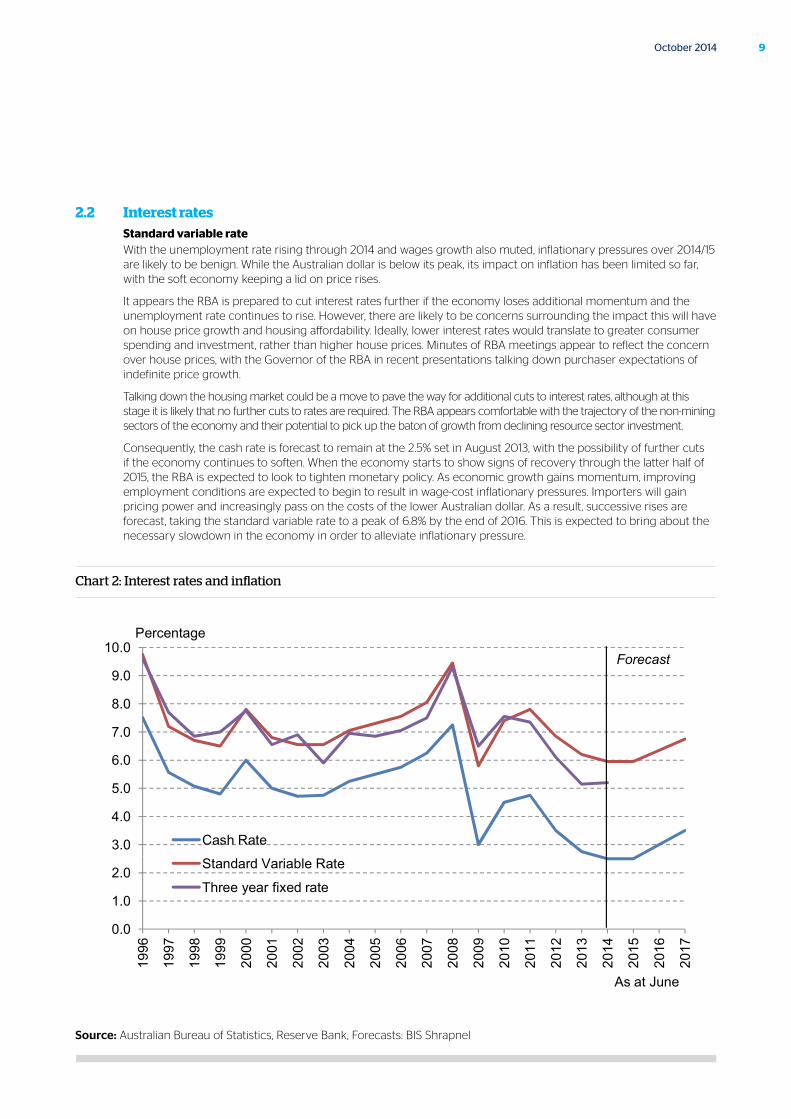
2.2 Interest rates Standard variable rate
With the unemployment rate rising through 2014 and wages growth also muted, inflationary pressures over 2014/15 are likely to be benign. While the Australian dollar is below its peak, its impact on inflation has been limited so far, with the soft economy keeping a lid on price rises.
It appears the RBA is prepared to cut interest rates further if the economy loses additional momentum and the unemployment rate continues to rise. However, there are likely to be concerns surrounding the impact this will have on house price growth and housing affordability. Ideally, lower interest rates would translate to greater consumer spending and investment, rather than higher house prices. Minutes of RBA meetings appear to reflect the concern over house prices, with the Governor of the RBA in recent presentations talking down purchaser expectations of indefinite price growth.
Talking down the housing market could be a move to pave the way for additional cuts to interest rates, although at this stage it is likely that no further cuts to rates are required. The RBA appears comfortable with the trajectory of the non-mining sectors of the economy and their potential to pick up the baton of growth from declining resource sector investment.
Consequently, the cash rate is forecast to remain at the 2.5% set in August 2013, with the possibility of further cuts if the economy continues to soften. When the economy starts to show signs of recovery through the latter half of 2015, the RBA is expected to look to tighten monetary policy. As economic growth gains momentum, improving employment conditions are expected to begin to result in wage-cost inflationary pressures. Importers will gain pricing power and increasingly pass on the costs of the lower Australian dollar. As a result, successive rises are forecast, taking the standard variable rate to a peak of 6.8% by the end of 2016. This is expected to bring about the necessary slowdown in the economy in order to alleviate inflationary pressure.
Chart 2: Interest rates and inflation
3.0
4.0
5.0
6.0
7.0
8.0
9.0
10.0
Cash Rate
Percentage
Forecast
0.0
1.0
2.0
1996
1997
1998
1999
2000
2001
2002
2003
2004
2005
2006
2007
2008
2009
2010
2011
2012
2013
2014
2015
2016
2017
Standard Variable Rate
Three year fixed rate
As at June
Source: Australian Bureau of Statistics, Reserve Bank, Forecasts: BIS Shrapnel
Other lending ratesMortgage interest rates are typically reported in terms of the standard variable rate. However, banks and other lenders also offer other lower interest rate options to borrowers, which in turn result in increased affordability (or greater purchasing power).
The gap between three-year fixed rates and the standard variable rate was at its maximum level at June 2013, with the three-year fixed rate being 101 basis points below the standard variable rate, or around 5.15% at June 2013. Three-year fixed rates are now factoring in an expected tightening in the interest rate cycle, with the margin below the standard variable rate narrowing to around 75 basis points by September 2014. At the same time, fixed rate loans fell from 19% of owner occupier lending at June 2013 to 14% in the three months to July 2014.
Banks also offer a discount to the standard variable rate to selected customers depending on size and characteristics of the loan. The RBA quotes an indicative discount of 85 basis points on the standard variable rate. However, this can exceed 100 basis points to selected mortgagors, taking the lending rate well below 5%.
These lower interest rates have increased the capacity of purchasers to pay, with Chart 3 showing affordability still at 2002 levels nationally for loans at the discounted variable rate. Moreover, given discounted rates are likely to apply to those in stable employment and on higher incomes, they will favour those purchasing dwellings in the middle to upper price ranges. This is typified by the price performance in the inner and middle suburbs of the capital cities (as highlighted in the capital cities section of this report).
10 Australian Housing Outlook 2014-17

Chart 3: Affordability*, standard variable rate and discounted variable rate, Australia
15.0
17.0
19.0
21.0
23.0
25.0
27.0
29.0
31.0
33.0
35.0
1991
1992
1993
1994
1995
1996
1997
1998
1999
2000
2001
2002
2003
2004
2005
2006
2007
2008
2009
2010
2011
2012
2013
2014
Discounted variable rate
Standard variable rate
Per cent
As at June quarter
Brief period of record low interest rates
Standard variable rate -affordabilty at 2003 levels
Discounted variable rate -affordabilty at 2002 levels
Source: Australian Bureau of Statistics, Reserve Bank, Forecasts: BIS Shrapnel
* based on mortgage repayments on 75% of the median house price as a percentage of household disposable income.
11October 2014

12 Australian Housing Outlook 2014-17
2.3 The rise of investors
The strength in many of Australia’s housing markets during the past 12 months has been characterised by the increased presence of investor purchasers in the market. The value of finance for residential investment has been steadily rising from just under 40% of total residential finance in the year to June 2011, to 45.2% in the year to June 2014 (Chart 4). The monthly share has consistently been in the 45% to 50% range since March 2014.
The low interest rate environment has narrowed the gap between rental income and mortgage outflows for investors, while recent price rises have encouraged the expectation of further capital growth. With low returns being offered by other investment classes such as fixed interest, current conditions have provided an attractive environment for investors.
While the rise in investor demand has generally been broad based, there are still noticeable differences in the strength of investor demand across the states. This is highlighted in Section 3.4.
Chart 4: Share of loans to residential purchasers by purchaser type, Australia
0.0
5.0
10.0
15.0
20.0
25.0
30.0
35.0
40.0
45.0
50.0
Jun-
03
Dec
-03
Jun-
04
Dec
-04
Jun-
05
Dec
-05
Jun-
06
Dec
-06
Jun-
07
Dec
-07
Jun-
08
Dec
-08
Jun-
09
Dec
-09
Jun-
10
Dec
-10
Jun-
11
Dec
-11
Jun-
12
Dec
-12
Jun-
13
Dec
-13
Jun-
14
First Home BuyersNon-First Home BuyersInvestors
Share of total residential loan value
Year ended month
Source: Australian Bureau of Statistics

13October 2014
14 Australian Housing Outlook 2014-17
3.1 Current trends
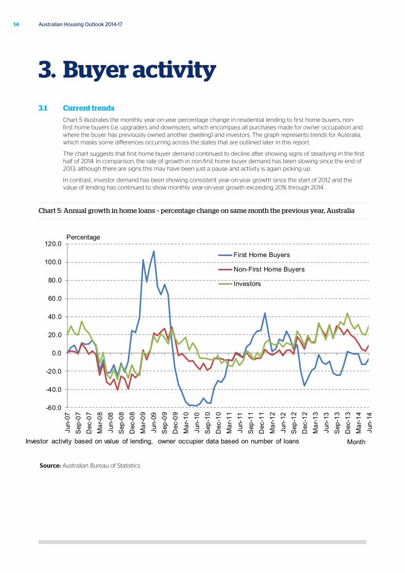
Chart 5 illustrates the monthly year-on-year percentage change in residential lending to first home buyers, non-first home buyers (i.e. upgraders and downsizers, which encompass all purchases made for owner occupation and where the buyer has previously owned another dwelling) and investors. The graph represents trends for Australia, which masks some differences occurring across the states that are outlined later in this report.
The chart suggests that first home buyer demand continued to decline after showing signs of steadying in the first half of 2014. In comparison, the rate of growth in non-first home buyer demand has been slowing since the end of 2013, although there are signs this may have been just a pause and activity is again picking up.
In contrast, investor demand has been showing consistent year-on-year growth since the start of 2012 and the value of lending has continued to show monthly year-on-year growth exceeding 20% through 2014.
Chart 5: Annual growth in home loans – percentage change on same month the previous year, Australia
-60.0
-40.0
-20.0
0.0
20.0
40.0
60.0
80.0
100.0
120.0
Jun-
07S
ep-0
7D
ec-0
7M
ar-0
8Ju
n-08
Sep
-08
Dec
-08
Mar
-09
Jun-
09S
ep-0
9D
ec-0
9M
ar-1
0Ju
n-10
Sep
-10
Dec
-10
Mar
-11
Jun-
11S
ep-1
1D
ec-1
1M
ar-1
2Ju
n-12
Sep
-12
Dec
-12
Mar
-13
Jun-
13S
ep-1
3D
ec-1
3M
ar-1
4Ju
n-14
First Home Buyers
Non-First Home Buyers
Investors
Percentage
MonthInvestor activity based on value of lending, owner occupier data based on number of loans
Source: Australian Bureau of Statistics
3. Buyer activity
15October 2014
3.2 First home buyers Incentives available
First home buyer demand is important as it creates demand for entry level properties, which then facilitates broader demand by encouraging current occupiers to upgrade through the value chain. As a result, governments have often used incentives to promote first home buyer demand during times of market weakness.
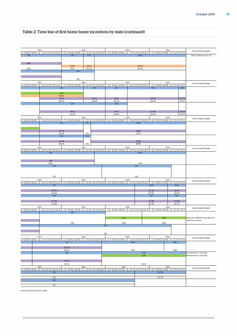
Table 2 shows the total State and Federal Government incentives offered to first home buyers since 2007. It refers to grants available specifically to first home buyers and not broader grants and incentives that first home buyers can also take advantage of. Where stamp duty concessions are offered, the maximum concession is indicated. Purchase price limits for grant eligibility have changed during this period and the incentives shown are for dwellings purchased below the price limit in place at the time.
Over the last three years there have been progressive changes in first home buyer incentives across all states and territories to favour purchasers of new homes over existing homes. The long-term impact will be a shift of some first home buyer demand that would have otherwise been for established homes into the new home market, thereby adding to supply.
However, there has been a short-term impact on the market as incentives for the purchase of established dwellings have been progressively removed:
• Future first home buyer demand has been brought forward to take advantage of the grants before they expire, leaving a vacuum of first home buyers in the established market immediately afterwards.
• There has been a delay in the next round of first home buyers who now have to accumulate a larger deposit to compensate for the lack of financial assistance.
The impact across the states has differed in line with the level of incentives being offered. An examination of Table 2 suggests the biggest losses in incentives for established homes from their recent peaks have been in New South Wales (total reduction of $25,000), Northern Territory (reduction of $21,700) and Queensland (reduction of $13,700). It is also these states that experienced the sharpest declines in loans to first home buyers from their previous peak (Chart 6).
Interestingly, Victoria has been experiencing sharp falls in first home buyer demand since the middle of 2013. This is despite the $7,000 First Home Owner’s Grant being replaced by a commensurate increase in the stamp duty concession. This would imply that a cash incentive has a greater impact than a similar sized non-cash incentive such as stamp duty savings. It may also explain the success of the First Home Owner’s Grant Boost Scheme in 2008.
In the Australian Capital Territory (ACT), removal of the $7,000 First Home Owner’s Grant in September 2013 has resulted in loans to first home buyers declining. Although more recent reductions to first home buyer incentives in Western Australia (WA), South Australia (SA) and Tasmania have seen activity initially rise, signs of a downturn in loans have emerged in the months following the reduction.

16 Australian Housing Outlook 2014-17
Table 2: Time line of first home buyer incentives by state
J F M A M J J A S O N D J F M A M J J A S O N D J F M A M J J A S O N D J F M A M J J A S O N D J F M A M J J A S O N D J F M A M J J A S O N D J F M A M J J A S OFirst Home Owner Grant $15K Falls to $10K from Jan '16First Home Owner Grant Boost SchemeNew Home Buyers SupplementFirst Home Plus SchemeFirst Home - New Home Scheme $20.2KTotal $35.2KFirst Home Owner GrantFirst Home Owner Grant Boost SchemeFirst Home Plus SchemeTotal
J F M A M J J A S O N D J F M A M J J A S O N D J F M A M J J A S O N D J F M A M J J A S O N D J F M A M J J A S O N D J F M A M J J A S O N D J F M A M J J A S OFirst Home Owner Grant $10K $10kFirst Home Owner Grant Boost SchemeFirst Home BonusFirst Home Owner Regional BonusStamp Duty Concessions $12.4K $15.5KTotal $22.4K $25.5kFirst Home Owner GrantFirst Home Owner Grant Boost SchemeFirst Home BonusStamp Duty Concessions $12.4K $15.5KTotal $12.4K $15.5k
J F M A M J J A S O N D J F M A M J J A S O N D J F M A M J J A S O N D J F M A M J J A S O N D J F M A M J J A S O N D J F M A M J J A S O N D J F M A M J J A S OFirst Home Owner Grant $15KFirst Home Owner Grant Boost SchemeRegional First Home Owner GrantStamp Duty Concessions $8.8KTotal $23KFirst Home Owner GrantFirst Home Owner Grant Boost SchemeStamp Duty ConcessionsTotal
J F M A M J J A S O N D J F M A M J J A S O N D J F M A M J J A S O N D J F M A M J J A S O N D J F M A M J J A S O N D J F M A M J J A S O N D J F M A M J J A S OFirst Home Owner Grant $15KFirst Home Owner Grant Boost SchemeFirst Home ConcessionFirst Home Bonus GrantTotal $15KFirst Home Owner Grant $5KFirst Home Owner Grant Boost SchemeFirst Home ConcessionFirst Home Bonus GrantTotal $5K
J F M A M J J A S O N D J F M A M J J A S O N D J F M A M J J A S O N D J F M A M J J A S O N D J F M A M J J A S O N D J F M A M J J A S O N D J F M A M J J A S OFirst Home Owner Grant $10K $10KFirst Home Owner Grant Boost SchemeStamp Duty Concessions $17.8K $14.4KTotal $27.8K $24.4KFirst Home Owner Grant $3K $3KFirst Home Owner Grant Boost SchemeStamp Duty Concessions $17.8K $14.4KTotal $21.8K $17.4K
J F M A M J J A S O N D J F M A M J J A S O N D J F M A M J J A S O N D J F M A M J J A S O N D J F M A M J J A S O N D J F M A M J J A S O N D J F M A M J J A S OFirst Home Owner GrantFirst Home Owner Grant Boost SchemeFirst Home Builder Boost $15K $30KStamp Duty ConcessionsTotal $15K $30KFirst Home Owner Grant $7KFirst Home Owner Grant Boost SchemeStamp Duty ConcessionsTotal $7K
J F M A M J J A S O N D J F M A M J J A S O N D J F M A M J J A S O N D J F M A M J J A S O N D J F M A M J J A S O N D J F M A M J J A S O N D J F M A M J J A S OFirst Home Owner Grant $25K $26KFirst Home Owner Grant Boost SchemeStamp Duty ConcessionsTotal $25K $26KFirst Home Owner Grant $12K Removed from 1 July 2015First Home Owner Grant - Non Urban Area $13K Removed from 1 July 2015First Home Owner Grant Boost SchemeStamp Duty Concessions
Total $25K
J F M A M J J A S O N D J F M A M J J A S O N D J F M A M J J A S O N D J F M A M J J A S O N D J F M A M J J A S O N D J F M A M J J A S O N D J F M A M J J A S OFirst Home Owner Grant $7k $12.5KFirst Home Owner Grant Boost SchemeTotal $7k $12.5KFirst Home Owner Grant $7kFirst Home Owner Grant Boost SchemeTotal $7k
Note: Grants included are those only available to first home buyers. Grants available to first home buyers and non-first home buyers are not includedNote: Stamp Duty Concessions refers to the saving on the highest threshold value where no stamp duty is applied. They are only indicative as for some states we were not able to assertain the highest threshold value or duty rate at a particular time to workout the exact saving
Reduced to $20K from Jan 2014 and $10k from Jul 2015
$15.4K $14K $10.5K$7K $3.5K
$7K $7K $7K$15.4K $21K $14K
2012 2013 Future Expiry/Changes
$15.5K $15.5K
$15.5K $15.5K
Future Expiry/Changes2008 2009 2010 2011
ACT
New$7K $7K $7K
2014
$14K $7K
Established
STATEDWELLING
TYPE GRANT2008 2009 2010 2011
Established
$7K $7K $7K $7K $7K $7K
$26.7K $26.7K
$22.5K $29.5K $26K $22.5K $33.7K $33.7K
$7K $3.5K$15.5K $15.5K
NT
New
$7K $7K $7K $7K $7K $7K
2014
$26.7K $26.7K$22.5K $36.5K $29.5K $22.5K $33.7K $43.7K
$14K $7K$15.5K $15.5K
STATEDWELLING
TYPE GRANT2012 2013
Established
$7K $7K $7K $7K$7K $3.5K
$4K $4K $4K $4K$11K $18K $14.5K $11K
$7K
$7K
2010 2011 2012
$4K $4K $4K $4K$11K $25K $18K $11K
$7K
$17.8K $17.8K $17.8K $17.8K
Future Expiry/Changes
TAS
New
$7K $7K $7K
$24.8K $31.8K $28.3K $24.8K
STATEDWELLING
TYPE GRANT2008 2009
Established
2013 2014
$7K$14K
WA
New
$7K $7K $7K $7K$14K
2014
$7K $3.5K$17.8K $17.8K $17.8K $17.8K
2013
$24.8K $38.8K $31.8K $24.8K$7K $7K $7K $7K
$7K
STATEDWELLING
TYPE GRANT2008 2009 2010 2011 2012 Future Expiry/Changes
Established
$7K $7K $7K $7K $7K $7K
$4K$9.1K $11K $18K $14.5K $11K
$7K $3.5K$2.1K
$4K $4K $4K$7K
2012
$4K $4K $4K $4K $8K$9.1K $11K $25K $18K $11K $15K
$8.8K $15.5K
Future Expiry/Changes
SA
New
$7K $7K $7K $7KSTATE
DWELLING TYPE GRANT
2008 2009 2010 2013 2014
$7K $7K$14K
Established
$7K$2.1K
2011
$7K
$15.8K $22.8K $19.3K $15.8K $22.5K $7K
$7K$7K $3.5K
$7K $7K $7K $7K $7K$15.8K $29.8K $22.8K $15.8K $19.8K $22.5K
$8.8K $8.8K $8.8K
2013 Future Expiry/Changes
QLD
New
$7K $7K $7K $7K $7K $7K $7K
2014
$8.8K$8.8K
$14K $7K$4K
$8.8K $8.8K $8.8K $8.8K $8.8K $15.5K
STATEDWELLING
TYPE GRANT2008 2009 2010 2011 2012
Established$9.3K
$12K $17K $16K $12.5K $9K $7K $13.2K $16.3K
$3K $3K $2K $2K $2K$6.2K
$7K $7K $7K$7K $7K$7K $7K $3.5K
$26.5K $32.7K $13.2K $16.3K$7K $7K $7K
$6.2k $6.2K $9.3K$12K $15K $29K $36.5K $29.5K $22.5K
$13K $13K$3K $3K $4.5K $4.5K $4.5K $6.5K $6.5K
$7K$14K $14K $7K
Future Expiry/Changes
VIC
New
$7K $7K $7K $7K $7K $7K
2013 2014
$5K $5K $5K $11K $11K $11K
$7K $7K $7K
$7K
STATEDWELLING
TYPE GRANT2008 2009 2010 2011 2012
Established
$7K $7K $7K $7K $7K$7K $3.5K
$25K $32K $28.5K $25K
$25K $42K $35K $28K $25K $25K
$18K $18K $18K $18K
$27.5K
$14K $7K
$18K$18K $20.2K
$3K $3K $3K
2011 2012 Future Expiry/Changes
NSW
New
$7K $7K $7K $7KSTATE
DWELLING TYPE GRANT
2008 2009 2010 20142013
$18K $18K $18K $18K
$7K $7K $7K
17October 2014
Table 2: Time line of first home buyer incentives by state (continued)
J F M A M J J A S O N D J F M A M J J A S O N D J F M A M J J A S O N D J F M A M J J A S O N D J F M A M J J A S O N D J F M A M J J A S O N D J F M A M J J A S OFirst Home Owner Grant $15K Falls to $10K from Jan '16First Home Owner Grant Boost SchemeNew Home Buyers SupplementFirst Home Plus SchemeFirst Home - New Home Scheme $20.2KTotal $35.2KFirst Home Owner GrantFirst Home Owner Grant Boost SchemeFirst Home Plus SchemeTotal
J F M A M J J A S O N D J F M A M J J A S O N D J F M A M J J A S O N D J F M A M J J A S O N D J F M A M J J A S O N D J F M A M J J A S O N D J F M A M J J A S OFirst Home Owner Grant $10K $10kFirst Home Owner Grant Boost SchemeFirst Home BonusFirst Home Owner Regional BonusStamp Duty Concessions $12.4K $15.5KTotal $22.4K $25.5kFirst Home Owner GrantFirst Home Owner Grant Boost SchemeFirst Home BonusStamp Duty Concessions $12.4K $15.5KTotal $12.4K $15.5k
J F M A M J J A S O N D J F M A M J J A S O N D J F M A M J J A S O N D J F M A M J J A S O N D J F M A M J J A S O N D J F M A M J J A S O N D J F M A M J J A S OFirst Home Owner Grant $15KFirst Home Owner Grant Boost SchemeRegional First Home Owner GrantStamp Duty Concessions $8.8KTotal $23KFirst Home Owner GrantFirst Home Owner Grant Boost SchemeStamp Duty ConcessionsTotal
J F M A M J J A S O N D J F M A M J J A S O N D J F M A M J J A S O N D J F M A M J J A S O N D J F M A M J J A S O N D J F M A M J J A S O N D J F M A M J J A S OFirst Home Owner Grant $15KFirst Home Owner Grant Boost SchemeFirst Home ConcessionFirst Home Bonus GrantTotal $15KFirst Home Owner Grant $5KFirst Home Owner Grant Boost SchemeFirst Home ConcessionFirst Home Bonus GrantTotal $5K
J F M A M J J A S O N D J F M A M J J A S O N D J F M A M J J A S O N D J F M A M J J A S O N D J F M A M J J A S O N D J F M A M J J A S O N D J F M A M J J A S OFirst Home Owner Grant $10K $10KFirst Home Owner Grant Boost SchemeStamp Duty Concessions $17.8K $14.4KTotal $27.8K $24.4KFirst Home Owner Grant $3K $3KFirst Home Owner Grant Boost SchemeStamp Duty Concessions $17.8K $14.4KTotal $21.8K $17.4K
J F M A M J J A S O N D J F M A M J J A S O N D J F M A M J J A S O N D J F M A M J J A S O N D J F M A M J J A S O N D J F M A M J J A S O N D J F M A M J J A S OFirst Home Owner GrantFirst Home Owner Grant Boost SchemeFirst Home Builder Boost $15K $30KStamp Duty ConcessionsTotal $15K $30KFirst Home Owner Grant $7KFirst Home Owner Grant Boost SchemeStamp Duty ConcessionsTotal $7K
J F M A M J J A S O N D J F M A M J J A S O N D J F M A M J J A S O N D J F M A M J J A S O N D J F M A M J J A S O N D J F M A M J J A S O N D J F M A M J J A S OFirst Home Owner Grant $25K $26KFirst Home Owner Grant Boost SchemeStamp Duty ConcessionsTotal $25K $26KFirst Home Owner Grant $12K Removed from 1 July 2015First Home Owner Grant - Non Urban Area $13K Removed from 1 July 2015First Home Owner Grant Boost SchemeStamp Duty Concessions
Total $25K
J F M A M J J A S O N D J F M A M J J A S O N D J F M A M J J A S O N D J F M A M J J A S O N D J F M A M J J A S O N D J F M A M J J A S O N D J F M A M J J A S OFirst Home Owner Grant $7k $12.5KFirst Home Owner Grant Boost SchemeTotal $7k $12.5KFirst Home Owner Grant $7kFirst Home Owner Grant Boost SchemeTotal $7k
Note: Grants included are those only available to first home buyers. Grants available to first home buyers and non-first home buyers are not includedNote: Stamp Duty Concessions refers to the saving on the highest threshold value where no stamp duty is applied. They are only indicative as for some states we were not able to assertain the highest threshold value or duty rate at a particular time to workout the exact saving
Reduced to $20K from Jan 2014 and $10k from Jul 2015
$15.4K $14K $10.5K$7K $3.5K
$7K $7K $7K$15.4K $21K $14K
2012 2013 Future Expiry/Changes
$15.5K $15.5K
$15.5K $15.5K
Future Expiry/Changes2008 2009 2010 2011
ACT
New$7K $7K $7K
2014
$14K $7K
Established
STATEDWELLING
TYPE GRANT2008 2009 2010 2011
Established
$7K $7K $7K $7K $7K $7K
$26.7K $26.7K
$22.5K $29.5K $26K $22.5K $33.7K $33.7K
$7K $3.5K$15.5K $15.5K
NT
New
$7K $7K $7K $7K $7K $7K
2014
$26.7K $26.7K$22.5K $36.5K $29.5K $22.5K $33.7K $43.7K
$14K $7K$15.5K $15.5K
STATEDWELLING
TYPE GRANT2012 2013
Established
$7K $7K $7K $7K$7K $3.5K
$4K $4K $4K $4K$11K $18K $14.5K $11K
$7K
$7K
2010 2011 2012
$4K $4K $4K $4K$11K $25K $18K $11K
$7K
$17.8K $17.8K $17.8K $17.8K
Future Expiry/Changes
TAS
New
$7K $7K $7K
$24.8K $31.8K $28.3K $24.8K
STATEDWELLING
TYPE GRANT2008 2009
Established
2013 2014
$7K$14K
WA
New
$7K $7K $7K $7K$14K
2014
$7K $3.5K$17.8K $17.8K $17.8K $17.8K
2013
$24.8K $38.8K $31.8K $24.8K$7K $7K $7K $7K
$7K
STATEDWELLING
TYPE GRANT2008 2009 2010 2011 2012 Future Expiry/Changes
Established
$7K $7K $7K $7K $7K $7K
$4K$9.1K $11K $18K $14.5K $11K
$7K $3.5K$2.1K
$4K $4K $4K$7K
2012
$4K $4K $4K $4K $8K$9.1K $11K $25K $18K $11K $15K
$8.8K $15.5K
Future Expiry/Changes
SA
New
$7K $7K $7K $7KSTATE
DWELLING TYPE GRANT
2008 2009 2010 2013 2014
$7K $7K$14K
Established
$7K$2.1K
2011
$7K
$15.8K $22.8K $19.3K $15.8K $22.5K $7K
$7K$7K $3.5K
$7K $7K $7K $7K $7K$15.8K $29.8K $22.8K $15.8K $19.8K $22.5K
$8.8K $8.8K $8.8K
2013 Future Expiry/Changes
QLD
New
$7K $7K $7K $7K $7K $7K $7K
2014
$8.8K$8.8K
$14K $7K$4K
$8.8K $8.8K $8.8K $8.8K $8.8K $15.5K
STATEDWELLING
TYPE GRANT2008 2009 2010 2011 2012
Established$9.3K
$12K $17K $16K $12.5K $9K $7K $13.2K $16.3K
$3K $3K $2K $2K $2K$6.2K
$7K $7K $7K$7K $7K$7K $7K $3.5K
$26.5K $32.7K $13.2K $16.3K$7K $7K $7K
$6.2k $6.2K $9.3K$12K $15K $29K $36.5K $29.5K $22.5K
$13K $13K$3K $3K $4.5K $4.5K $4.5K $6.5K $6.5K
$7K$14K $14K $7K
Future Expiry/Changes
VIC
New
$7K $7K $7K $7K $7K $7K
2013 2014
$5K $5K $5K $11K $11K $11K
$7K $7K $7K
$7K
STATEDWELLING
TYPE GRANT2008 2009 2010 2011 2012
Established
$7K $7K $7K $7K $7K$7K $3.5K
$25K $32K $28.5K $25K
$25K $42K $35K $28K $25K $25K
$18K $18K $18K $18K
$27.5K
$14K $7K
$18K$18K $20.2K
$3K $3K $3K
2011 2012 Future Expiry/Changes
NSW
New
$7K $7K $7K $7KSTATE
DWELLING TYPE GRANT
2008 2009 2010 20142013
$18K $18K $18K $18K
$7K $7K $7K

18 Australian Housing Outlook 2014-17
However, with first home owner demand being fixed (i.e. most households are a first home buyer at some stage), incentives do not create or diminish demand but rather serve to shift existing demand around over time. Once the impacts of the changes to incentives are worked through, first home buyer demand should return to long-term averages. With New South Wales (NSW), Queensland and, to a lesser extent, the Northern Territory (NT) being the first states to reduce incentives to first home buyers of established dwellings, this is evident in the emerging recovery in first home buyer demand in these markets.
The data on loans to first home buyers provided by the Australian Bureau of Statistics (ABS) are derived from returns submitted to the Australian Prudential Regulation Authority. First home buyers are defined as “a borrower entering the home ownership market for the first time”. Consequently, it encompasses all loans to first home buyers and not just those eligible for grants. It also excludes first home buyers who are investors as the data are provided in relation to loans for owner occupation.
Chart 6: Number of loans to first home buyers by state, moving annual totals
0
2,000
4,000
6,000
8,000
10,000
12,000
14,000
0
500
1,000
1,500
2,000
2,500
3,000
3,500
Jun-
07D
ec-0
7Ju
n-08
Dec
-08
Jun-
09D
ec-0
9Ju
n-10
Dec
-10
Jun-
11D
ec-1
1Ju
n-12
Dec
-12
Jun-
13D
ec-1
3Ju
n-14
TASNTACTSA (RHS)
FHOG Boost Scheme
Major policy changes
Source: Australian Bureau of Statistics
0
10,000
20,000
30,000
40,000
50,000
60,000
70,000
Jun-
07D
ec-0
7Ju
n-08
Dec
-08
Jun-
09D
ec-0
9Ju
n-10
Dec
-10
Jun-
11D
ec-1
1Ju
n-12
Dec
-12
Jun-
13D
ec-1
3Ju
n-14
NSWVICQLDWA
FHOG Boost Scheme
Major policy changes

19October 2014
3.3 Upgraders (and downsizers)
Upgraders and downsizers represent the largest component of residential demand, at around two to three times the size of the first home buyer market, and currently represent around 45% of total residential lending activity.
In particular, upgrader demand has been strengthening since bottoming out in 2011 or 2012 in all states. However, Victoria is the only state where the number of loans to upgraders is exceeding the pre-GFC levels of 2007, with NSW and the ACT the only other states reporting upgrader activity close to 2007 levels.
• The solid growth apparent in loans to upgraders in NSW, Victoria and the ACT in 2013/14 has been joined by healthy rises in Queensland, Tasmania and SA, although the latter states are still tracking at historically low levels of demand. Should this trend continue, the increase in activity is likely to translate to stronger price growth emerging in these markets.
• In contrast, loans to upgraders have only recorded more modest rises in WA and the NT. Despite strong price growth in both Perth and Darwin in 2013, it was investor activity in both states (and first home buyer activity in WA) that drove change. Price rises in both capital cities are now slowing over 2013/14.
Chart 7: Number of loans to upgraders and downsizers by state, moving annual totals
0
20,000
40,000
60,000
80,000
100,000
120,000
Jun-
07D
ec-0
7Ju
n-08
Dec
-08
Jun-
09D
ec-0
9Ju
n-10
Dec
-10
Jun-
11D
ec-1
1Ju
n-12
Dec
-12
Jun-
13D
ec-1
3Ju
n-14
NSW
VIC
QLD
WA
0
5,000
10,000
15,000
20,000
25,000
30,000
35,000
0
1,000
2,000
3,000
4,000
5,000
6,000
7,000
8,000
9,000
10,000
Jun-
07D
ec-0
7Ju
n-08
Dec
-08
Jun-
09D
ec-0
9Ju
n-10
Dec
-10
Jun-
11D
ec-1
1Ju
n-12
Dec
-12
Jun-
13D
ec-1
3Ju
n-14
TASNTACTSA (RHS)
Source: Australian Bureau of Statistics
20 Australian Housing Outlook 2014-17
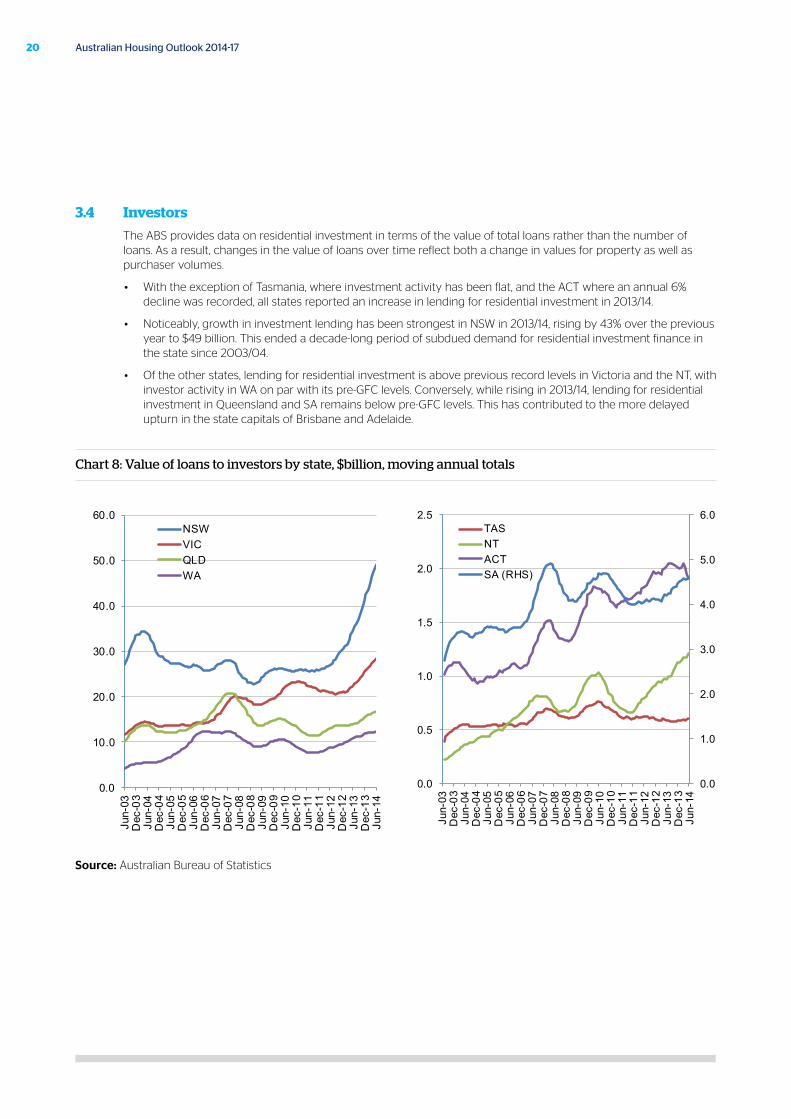
3.4 Investors
The ABS provides data on residential investment in terms of the value of total loans rather than the number of loans. As a result, changes in the value of loans over time reflect both a change in values for property as well as purchaser volumes.
• With the exception of Tasmania, where investment activity has been flat, and the ACT where an annual 6% decline was recorded, all states reported an increase in lending for residential investment in 2013/14.
• Noticeably, growth in investment lending has been strongest in NSW in 2013/14, rising by 43% over the previous year to $49 billion. This ended a decade-long period of subdued demand for residential investment finance in the state since 2003/04.
• Of the other states, lending for residential investment is above previous record levels in Victoria and the NT, with investor activity in WA on par with its pre-GFC levels. Conversely, while rising in 2013/14, lending for residential investment in Queensland and SA remains below pre-GFC levels. This has contributed to the more delayed upturn in the state capitals of Brisbane and Adelaide.
Chart 8: Value of loans to investors by state, $billion, moving annual totals
0.0
10.0
20.0
30.0
40.0
50.0
60.0
Jun-
03D
ec-0
3Ju
n-04
Dec
-04
Jun-
05D
ec-0
5Ju
n-06
Dec
-06
Jun-
07D
ec-0
7Ju
n-08
Dec
-08
Jun-
09D
ec-0
9Ju
n-10
Dec
-10
Jun-
11D
ec-1
1Ju
n-12
Dec
-12
Jun-
13D
ec-1
3Ju
n-14
NSWVICQLDWA
0.0
1.0
2.0
3.0
4.0
5.0
6.0
0.0
0.5
1.0
1.5
2.0
2.5
Jun-
03D
ec-0
3Ju
n-04
Dec
-04
Jun-
05D
ec-0
5Ju
n-06
Dec
-06
Jun-
07D
ec-0
7Ju
n-08
Dec
-08
Jun-
09D
ec-0
9Ju
n-10
Dec
-10
Jun-
11D
ec-1
1Ju
n-12
Dec
-12
Jun-
13D
ec-1
3Ju
n-14
TASNTACTSA (RHS)
Source: Australian Bureau of Statistics

21October 2014
4.1 Vacancy rates
The vacancy rate in each city reflects the level of rental oversupply or deficiency. A vacancy rate of 3% in a market is considered balanced, where rents on average will rise roughly in line with inflation.
• Although rising in the year to June 2014 to 2.4%, vacancy rates in Brisbane have been below 3% since 2011 and reflect a tight market. Vacancy rates in Sydney have also been consistently tight and below 3% since 2005. Interestingly, Melbourne’s vacancy rate has tightened from 3.4% at June 2013 to 2.8% at June 2014, reversing the steadily rising trend since 2008. This is despite the high level of new dwelling activity taking place. Migration (both overseas and interstate) into Victoria is very strong and working to offset the addition of new supply.
• Vacancy rates in Perth have followed cycles in both mining investment and supply, tightening from 4.3% at June 2010 to 1.9% in June 2012, before rising again to 4.2% at June 2014. While new dwelling completions have been rising, population numbers would suggest an overall dwelling deficiency is still in place. Consequently, the rise in vacancy rates could reflect the time taken to “back fill” rental stock. Strong first home buyer numbers in the State and falling migration levels are causing an exit from rental properties, and the pace of new rental tenants coming to the market may be failing to keep up. Alternatively, the nature of temporary overseas migration into WA may suggest these population flows haven’t necessarily translated into lasting demand for housing.
• Vacancy rates in Adelaide and Hobart have been tightening from levels well above 3% as at June 2012. The attractive incentives to first home buyers in both these states for new construction (and SA offers an additional incentive for new construction for all market segments) are contributing to a recovery in new dwelling activity. There is a risk that vacancy rates will trend upwards again over 2014/15 as these dwellings work their way through to completion.
• Canberra and Darwin’s rental vacancy rates have risen over the year to be above 4% at June 2014. Record levels of new apartment commencements in recent years are now translating to new rental supply, with the NT market estimated to be shifting from an estimated deficiency into oversupply over 2014/15. The ACT is estimated to be already experiencing a rising excess of dwelling stock.
Chart 9: Residential vacancy rates
0.0
0.5
1.0
1.5
2.0
2.5
3.0
3.5
4.0
4.5
5.0
2002
2003
2004
2005
2006
2007
2008
2009
2010
2011
2012
2013
2014
Sydney
Melbourne
Brisbane
Perth
Balancedmarket = 3%
Per cent
0.0
1.0
2.0
3.0
4.0
5.0
6.0
7.0
8.0
2002
2003
2004
2005
2006
2007
2008
2009
2010
2011
2012
2013
2014
Adelaide
Hobart
Canberra
Darwin
Balancedmarket = 3%
Per cent
Source: Real Estate Institute of Australia
4. Rental markets

22 Australian Housing Outlook 2014-17
4.2 Rental growth
Rental growth was strong in the latter half of the 2000s after a period of underperformance in the first half of the decade. In more recent years, rental growth has generally been more moderate, despite vacancy rates remaining tight in many capital cities. This suggests that there may be some rental affordability constraints preventing stronger rises.
• In particular, rental growth has slowed to around 2% in Melbourne, Brisbane, Adelaide and Hobart, which is below the level of inflation. In Melbourne, Adelaide and Hobart, this reflects vacancy rates at or around the balanced market rate of 3%, while in Brisbane it may be an indication of current economic and employment conditions. Rental growth in Sydney has also slowed, although not to the same extent, to 3.0% in 2013/14.
• Rental growth in both Perth and Darwin has slowed to 2.9% and 4.8% respectively in 2013/14 after both recording 7.5% increases in 2012/13. The strong growth occurred in response to low vacancy rates, a strong state economy and healthy employment conditions. However, supply is now rising in both states, while migration and underlying demand is slowing and resource sector investment is weakening. As a result, lower rates of rental growth are expected in 2014/15.
• Rents in Canberra have actually fallen by 0.8% in 2013/14, reflecting the high level of vacancy rates.
Chart 10: Annual rental growth
0.0
2.0
4.0
6.0
8.0
10.0
12.0
14.0
2002
2003
2004
2005
2006
2007
2008
2009
2010
2011
2012
2013
2014
Sydney
Melbourne
Brisbane
Perth
Per cent
-2.0
0.0
2.0
4.0
6.0
8.0
10.0
12.0
14.0
2002
2003
2004
2005
2006
2007
2008
2009
2010
2011
2012
2013
2014
AdelaideHobartCanberraDarwin
Per cent
Source: Australian Bureau of Statistics

23October 2014
5. YieldsChart 11 shows movement in indicative rental yields for houses by capital city. This figure is calculated by the median three-bedroom house rent divided by the median house price. The indicative yield slightly understates actual yields, as the median three-bedroom rent is calculated for investment houses, which would typically be priced below the median house price. Nevertheless, movement in the indicative yield should correspond with actual yields. A comparison is made with the standard variable interest rate to compare the rental return with the cost of financing.
• With the exception of Adelaide, where yields were steady, indicative yields have deteriorated across all other capital cities in 2013/14. However, the causes vary. Yields in Sydney, Melbourne and Brisbane fell due to solid price growth, while weaker rents contributed to lower yields in Perth, Hobart, Canberra and Darwin.
• In Sydney and Perth, yields still remain considerably higher than the levels of the early to mid 2000s. For Brisbane, yields have been relatively steady since their low point in 2004, although well below levels at the start of the decade. Indicative yields in Melbourne have fallen below 3% for the first time since at least 2002.
• Adelaide, Hobart, Canberra and Darwin typically have higher yields than Sydney or Melbourne. Like Brisbane, yields are generally lower than at the start of the 2000s, perhaps reflecting a sustained shift in these markets’ response to a lower interest rate environment. Being such a small and volatile market, Darwin has the highest indicative yields of the capital cities.
Despite the low indicative yields, low mortgage interest rates mean the gap between rental yields and interest rates in most capital cities remains narrow in a long term sense. In some instances, selected properties in individual markets are also likely to be positively geared, particularly where discounted mortgage rates are on offer. This narrowed gap, together with the emergence of capital growth in many capital cities in 2013/14, is expected to remain attractive to investors and drive further increases in investor demand across most states over 2014/15
Chart 11: Standard variable interest rate and indicative rental yields by capital city, houses
0.0
1.0
2.0
3.0
4.0
5.0
6.0
7.0
8.0
9.0
10.0
2000
2001
2002
2003
2004
2005
2006
2007
2008
2009
2010
2011
2012
2013
2014
SydneyMelbourneBrisbanePerthVariable rate
Per cent
0.0
1.0
2.0
3.0
4.0
5.0
6.0
7.0
8.0
9.0
10.0
2000
2001
2002
2003
2004
2005
2006
2007
2008
2009
2010
2011
2012
2013
2014
AdelaideHobartCanberraDarwinVariable rate
Per cent
Source: Real Estate Institute of Australia, Reserve Bank
24 Australian Housing Outlook 2014-17
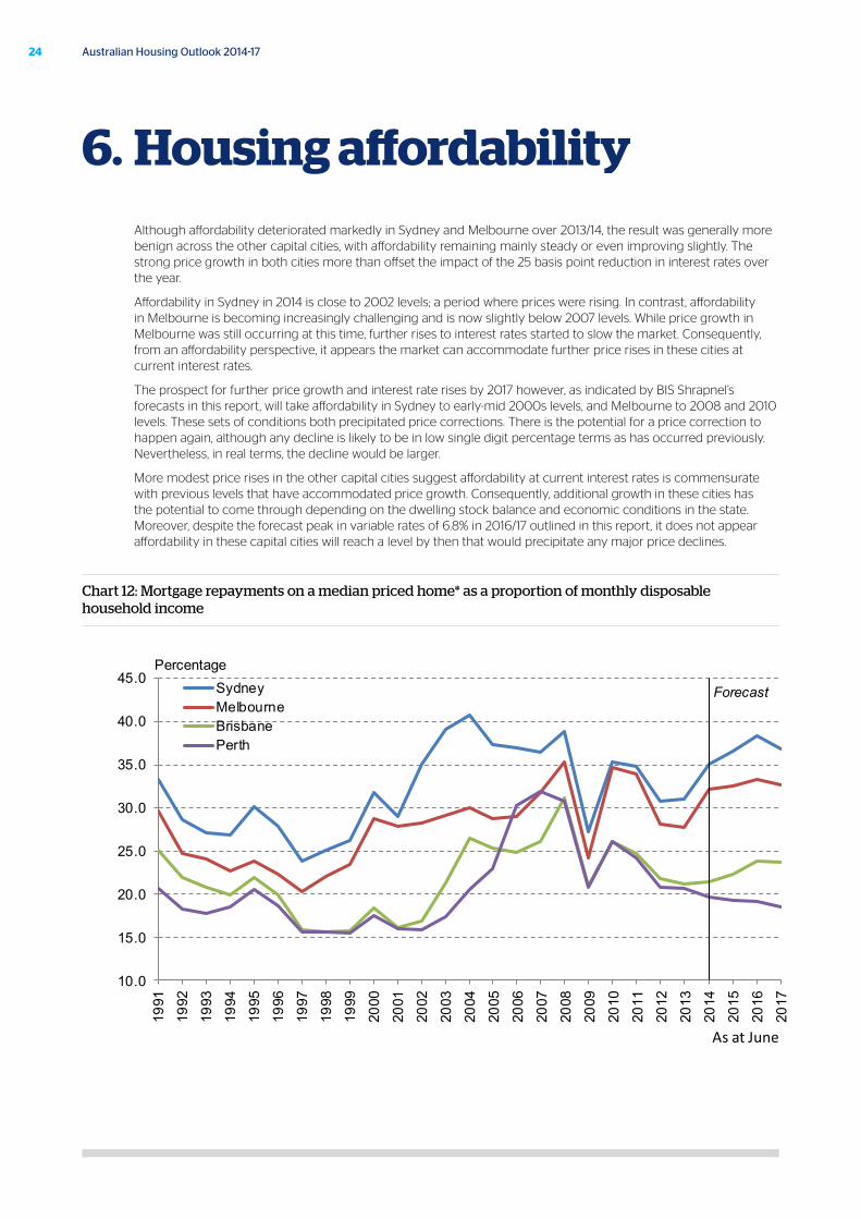
Although affordability deteriorated markedly in Sydney and Melbourne over 2013/14, the result was generally more benign across the other capital cities, with affordability remaining mainly steady or even improving slightly. The strong price growth in both cities more than offset the impact of the 25 basis point reduction in interest rates over the year.
Affordability in Sydney in 2014 is close to 2002 levels; a period where prices were rising. In contrast, affordability in Melbourne is becoming increasingly challenging and is now slightly below 2007 levels. While price growth in Melbourne was still occurring at this time, further rises to interest rates started to slow the market. Consequently, from an affordability perspective, it appears the market can accommodate further price rises in these cities at current interest rates.
The prospect for further price growth and interest rate rises by 2017 however, as indicated by BIS Shrapnel’s forecasts in this report, will take affordability in Sydney to early-mid 2000s levels, and Melbourne to 2008 and 2010 levels. These sets of conditions both precipitated price corrections. There is the potential for a price correction to happen again, although any decline is likely to be in low single digit percentage terms as has occurred previously. Nevertheless, in real terms, the decline would be larger.
More modest price rises in the other capital cities suggest affordability at current interest rates is commensurate with previous levels that have accommodated price growth. Consequently, additional growth in these cities has the potential to come through depending on the dwelling stock balance and economic conditions in the state. Moreover, despite the forecast peak in variable rates of 6.8% in 2016/17 outlined in this report, it does not appear affordability in these capital cities will reach a level by then that would precipitate any major price declines.
Chart 12: Mortgage repayments on a median priced home* as a proportion of monthly disposable household income
10.0
15.0
20.0
25.0
30.0
35.0
40.0
45.0
1991
1992
1993
1994
1995
1996
1997
1998
1999
2000
2001
2002
2003
2004
2005
2006
2007
2008
2009
2010
2011
2012
2013
2014
2015
2016
2017
SydneyMelbourneBrisbanePerth
Percentage
As at June
Forecast
6. Housing affordability

25October 2014
Chart 12 (cont.): Mortgage repayments on a median priced home* as a proportion of monthly disposable household income
10.0
15.0
20.0
25.0
30.0
35.0
40.0
45.0
1991
1992
1993
1994
1995
1996
1997
1998
1999
2000
2001
2002
2003
2004
2005
2006
2007
2008
2009
2010
2011
2012
2013
2014
2015
2016
2017
AdelaideHobartCanberraDarwin
Percentage
As at June
Forecast
Source: Australian Bureau of Statistics, Reserve Bank, Real Estate Institute of Australia, Forecasts: BIS Shrapnel
* Mortgage repayment based on 75% of the median house price

26 Australian Housing Outlook 2014-17
Underlying demand for new dwellings is driven primarily by population growth which, at the state level, comes from the combination of natural increase (births less deaths) and net overseas and net interstate migration flows. In particular, demand from net overseas and net interstate migration is more immediate as this group will require accommodation upon arrival, be it owner occupation or rental.
7.1 Overseas migration
Net overseas migration into Australia peaked at 315,000 in the year to December 2008. As well as permanent migration, the strong inflow was largely due to growth in temporary (although long-term) overseas migrants, predominantly those on student or skilled temporary (subclass 457) visas.
The correction through to 2010 (with national net overseas migration falling to 172,000 persons) was not only caused by the decline in arrivals resulting from weaker local economic conditions, but also rising long-term departures as temporary migrants that drove earlier record net overseas migration returned to their country of origin.
The recovery to a net overseas migration of 242,800 in 2012/13 was underpinned largely by a rebound in arrivals, which surpassed the previous peak. However, with arrivals now trending downwards as resource sector investment and the Australian economy slows, net overseas migration flows have weakened to 235,800 in the year to December 2013. This trend is forecast to accelerate over the next three years. Arrivals will slow and departures should increase due to the lack of opportunities for temporary migrants to extend their stay. As a result, it is forecast that net overseas migration is forecast to ease to 150,000 persons nationally by 2016/17. While well down since the peak in 2009, it is higher than all but one year prior to 2006/07
Chart 13: Arrivals and departures (movements) and net overseas migration (persons), moving annual totals, Australia
100
200
300
400
500
600
700
800
900
0
50
100
150
200
250
300
350
400
450
Jun-
00D
ec-0
0Ju
n-01
Dec
-01
Jun-
02D
ec-0
2Ju
n-03
Dec
-03
Jun-
04D
ec-0
4Ju
n-05
Dec
-05
Jun-
06D
ec-0
6Ju
n-07
Dec
-07
Jun-
08D
ec-0
8Ju
n-09
Dec
-09
Jun-
10D
ec-1
0Ju
n-11
Dec
-11
Jun-
12D
ec-1
2Ju
n-13
Dec
-13
Jun-
14Permanent and long term departuresNet Overseas MigrationPermanent and long term arrivals (RHS)
Persons ('000s)
Year EndingSource: Australian Bureau of Statistics, BIS Shrapnel
Persons ('000s)
7. Demand

27October 2014
With the most recent peak in net overseas migration in 2012/13 fuelled by the rise in subclass 457 visa entrants, the main beneficiaries have been WA and the NT. These states experienced the greatest skills shortages emerging from their high level of resource sector investment and also witnessed record net overseas migration in 2012/13.
While all states are forecast to experience a fall in net overseas migration inflows through to 2016/17, in line with the national total, the greatest declines will be felt in the resource sector states (WA, the NT and, to a lesser extent, Queensland). It is believed the high concentration of temporary migration will result in increased outflows as investment projects wind down and employment slows. In contrast, net overseas migration in the states that have benefited less from temporary migrants – including NSW, Victoria, SA, Tasmania and the ACT – should experience a softer decline.
Chart 14: Annual net overseas migration by state
0.0
10.0
20.0
30.0
40.0
50.0
60.0
70.0
80.0
90.0
100.0
1999
2000
2001
2002
2003
2004
2005
2006
2007
2008
2009
2010
2011
2012
2013
2014
e20
1520
1620
17
NSWVICQLDWA
Persons ('000s)
Year ended JuneSource: Australian Bureau of Statistics, BIS Shrapnel
Forecast
0.0
2.0
4.0
6.0
8.0
10.0
12.0
14.0
16.0
18.0
20.0
-0.5
0.0
0.5
1.0
1.5
2.0
2.5
3.0
3.5
4.0
1999
2000
2001
2002
2003
2004
2005
2006
2007
2008
2009
2010
2011
2012
2013
2014
e20
1520
1620
17
TASNTACTSA (RHS)
Persons ('000s)
Year ended JuneSource: Australian Bureau of Statistics, BIS Shrapnel
Forecast
Persons ('000s)

28 Australian Housing Outlook 2014-17
7.2 Interstate migration
The main drivers of migration between the states are relative housing affordability and economic conditions. Reduced interstate movement also generally occurs when economic conditions deteriorate overall, i.e. limited job prospects elsewhere encourage people to stay where they are.
• Queensland’s net interstate migration inflow has been at long-term lows in recent years, reflecting a period of both high relative house prices and weak economic performance. However, interstate migration is expected to begin to recover from 2014/15. This is in response to improved relative house price affordability following recent weak price growth in comparison to the stronger southern states.
• After falling markedly since peaking in 2003, the NSW net interstate outflow has improved but, as with 2003, rising house prices and deteriorating affordability in Sydney are likely to see the outflow increase. Victoria’s net inflow has also improved to record levels, estimated at 8,000 persons in 2013/14. However, with the State facing economic headwinds and a higher unemployment rate than the national level, the net inflow is likely to ease from 2014/15.
• Weakening employment conditions as resource sector investment winds down is forecast to see WA’s net interstate migration inflow revert to an outflow, while spending cuts to the public sector in the ACT is having the same effect there.
• The SA and Tasmanian net interstate migration outflows are likely to persist, though inflows into Tasmania may benefit from rising mainland house prices.
• The NT is currently experiencing a net interstate migration outflow despite the level of resource sector investment taking place. It could be that the high net overseas migration into the Territory has been accommodating the necessary skills requirements, leaving little demand for labour from interstate. Nevertheless, numbers have improved from a peak net outflow in 2010/11 and it is expected that the high level of investment activity will see this trend continue.
Chart 15: Annual net interstate migration by state
-40.0
-30.0
-20.0
-10.0
0.0
10.0
20.0
30.0
40.0
50.0
1999
2000
2001
2002
2003
2004
2005
2006
2007
2008
2009
2010
2011
2012
2013
2014
e20
1520
1620
17
NSW
VIC
QLD
WA
Persons ('000s)
Year ended JuneSource: Australian Bureau of Statistics, BIS Shrapnel
Forecast
-5.0
-4.0
-3.0
-2.0
-1.0
0.0
1.0
2.0
3.0
1999
2000
2001
2002
2003
2004
2005
2006
2007
2008
2009
2010
2011
2012
2013
2014
e20
1520
1620
17TAS
NT
ACT
SA
Persons ('000s)
Year ended JuneSource: Australian Bureau of Statistics, BIS Shrapnel
Forecast

29October 2014
7.3 Demand and supply
The underlying demand for new dwellings is driven largely by the formation of additional households, which in turn is largely underpinned by population growth. The balance between underlying demand and supply has an impact on vacancy rates, rents, prices and construction.
Chart 16 shows the forecast average underlying demand for additional dwellings by state over the next three years, compared with current supply, as indicated by total new dwelling commencements in 2013/14.
The upturn in new dwelling commencements in 2013/14 has taken new supply above average underlying demand in almost all states. The exception is Queensland. This should result in any deficiency in dwelling stock now beginning to be absorbed, or a rising excess in the states estimated to be in oversupply. The states where commencements are now highest relative to underlying demand are the ACT, WA, SA and the NT
Chart 16: Annual underlying demand and supply by state
0.0
10.0
20.0
30.0
40.0
50.0
60.0
NSW VIC QLD WA
Ave Ann Underlying Demand2014/15 to 2016/17Dwelling Commencements 2013/14
Dwellings ('000s)
0.0
2.0
4.0
6.0
8.0
10.0
12.0
SA TAS NT ACT
Ave Ann Underlying Demand2014/15 to 2016/17Dwelling Commencements 2013/14
Dwellings ('000s)
Source: Australian Bureau of Statistics, BIS Shrapnel, Forecasts: BIS Shrapnel
30 Australian Housing Outlook 2014-17
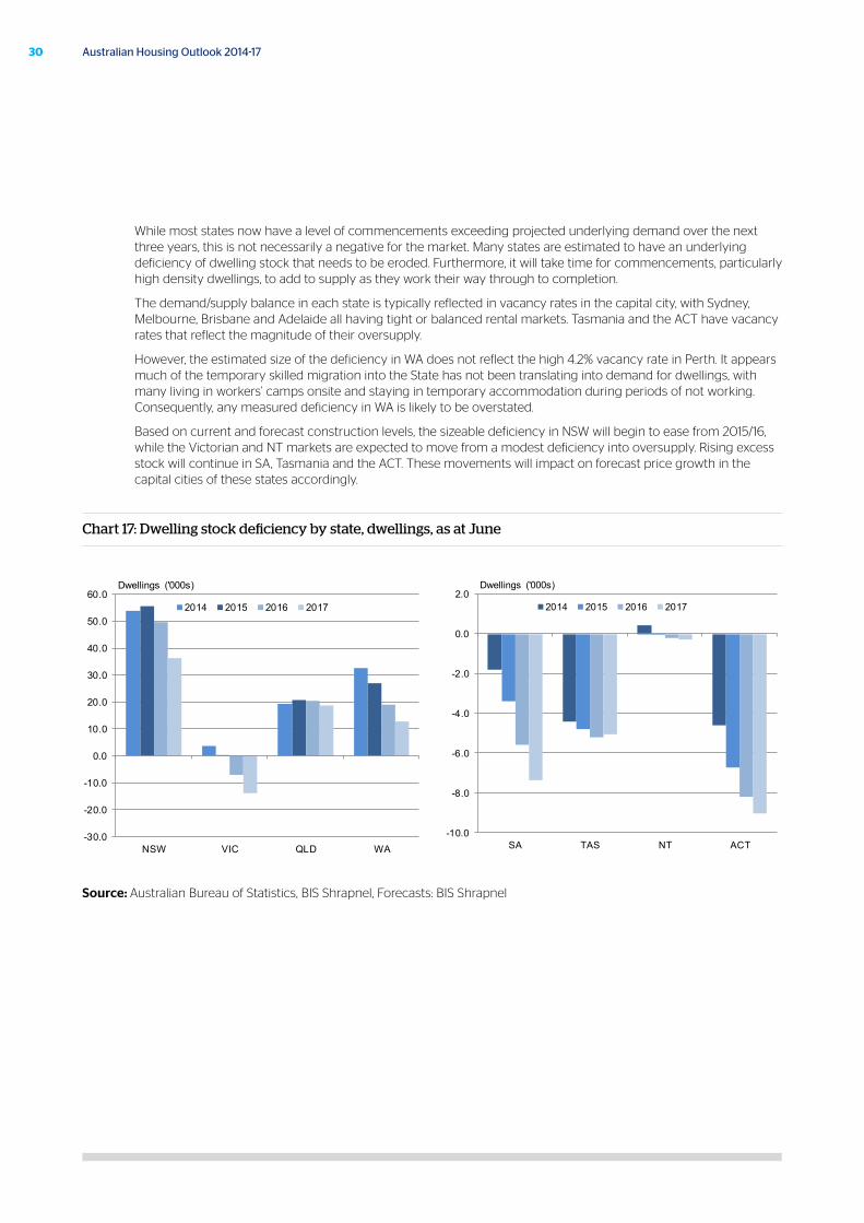
While most states now have a level of commencements exceeding projected underlying demand over the next three years, this is not necessarily a negative for the market. Many states are estimated to have an underlying deficiency of dwelling stock that needs to be eroded. Furthermore, it will take time for commencements, particularly high density dwellings, to add to supply as they work their way through to completion.
The demand/supply balance in each state is typically reflected in vacancy rates in the capital city, with Sydney, Melbourne, Brisbane and Adelaide all having tight or balanced rental markets. Tasmania and the ACT have vacancy rates that reflect the magnitude of their oversupply.
However, the estimated size of the deficiency in WA does not reflect the high 4.2% vacancy rate in Perth. It appears much of the temporary skilled migration into the State has not been translating into demand for dwellings, with many living in workers’ camps onsite and staying in temporary accommodation during periods of not working. Consequently, any measured deficiency in WA is likely to be overstated.
Based on current and forecast construction levels, the sizeable deficiency in NSW will begin to ease from 2015/16, while the Victorian and NT markets are expected to move from a modest deficiency into oversupply. Rising excess stock will continue in SA, Tasmania and the ACT. These movements will impact on forecast price growth in the capital cities of these states accordingly.
Chart 17: Dwelling stock deficiency by state, dwellings, as at June
-30.0
-20.0
-10.0
0.0
10.0
20.0
30.0
40.0
50.0
60.0
NSW VIC QLD WA
2014 2015 2016 2017
Dwellings ('000s)
-10.0
-8.0
-6.0
-4.0
-2.0
0.0
2.0
SA TAS NT ACT
2014 2015 2016 2017
Dwellings ('000s)
Source: Australian Bureau of Statistics, BIS Shrapnel, Forecasts: BIS Shrapnel
31October 2014
8. Capital city overviews and price forecasts

32 Australian Housing Outlook 2014-17
This section provides an overview of the residential markets of each of Australia’s state and territory capital cities and selected regional centres. An outlook is also provided, with the performance of the residential market measured by historical and forecast movement in the median house price.
In addition to the median house price, the report refers to the “real” median house price. This is the median house price after accounting for the impact of inflation. The real median house price allows for a better comparison of price growth over time as, during periods of high inflation, significant rises in the median house price may be underpinned by the inflation rate and not necessarily reflect a strong market.
8.1 Sydney
The increase in Sydney’s dwelling deficiency since the mid 2000s, and the easing in interest rate policy since the end of 2011, were the catalyst for the upturn in the Sydney residential market. After being largely flat over 2011/12, median house price growth in Sydney has accelerated from 7% in 2012/13 to 17% in 2013/14. While the first leg of the upturn emerged in inner Sydney over 2012/13, price growth became more broad based over 2013/14. Inner Sydney recorded the lowest rate of growth (+10.2%), with stronger growth now coming through in the middle (+17.3%) and outer-ring suburbs (+15.6%).
Median house price growth in Sydney by region, per cent, 2013/14
INNER MIDDLE OUTER MEDIAN
Annual % increase 10.2 17.3 15.6 17.0
Source: Real Estate Institute of Australia
With interest rates predicted to remain steady at their current levels over 2014/15, Sydney house price growth is forecast to continue, although at a slower rate than in 2013/14. There is still a sizeable dwelling deficiency in NSW and signs suggest first home buyer demand is beginning to strengthen. However, affordability has deteriorated, owner occupier demand appears to have topped out and more moderate growth in investor demand is expected from its current, very elevated, levels.
Price growth totalling 13% is forecast over 2014/15 and 2015/16, with some upside expected in the outer suburbs as demand shifts towards houses in more affordable locations. However, the rate of growth is expected to begin slowing through 2015/16. NSW’s stock deficiency is expected to begin to ease over 2015/16, while affordability constraints are also expected to come to the fore as interest rate policy is tightened and variable rates rise.
Consequently, Sydney’s median house price is forecast to peak at $915,000 by June 2016. Together with the forecast rise in variable rates to a peak of 6.8% by the end of 2016, affordability is expected to reach levels similar to the middle of last decade and a correction in the median house price of 3% is projected over 2016/17. This will take total growth to 9% over the three years to June 2017 and the median house price to $885,000. In real terms, Sydney’s median house price at June 2017 is forecast to be unchanged from June 2014 levels.

33October 2014
Chart 18: Sydney dwellings, prices and activity
+5+14
+4 +2 -6+7
+17+7
+5-3
+29
+22+7
+12-7
20
40
80
160
320
640
1,280
94 95 96 97 98 99 00 01 02 03 04 05 06 07 08 09 10 11 12 13 14 15 16 17
Year ended June Source: BIS Shrapnel, ABS & REIA data
Real house price Sydney ($'000)
House price Sydney ($'000)
Commencements ('000) New South Wales (Quarterly, MAT)
Average value of home loan ($'000)
Forecast
34 Australian Housing Outlook 2014-17
8.2 Regional NSW centres
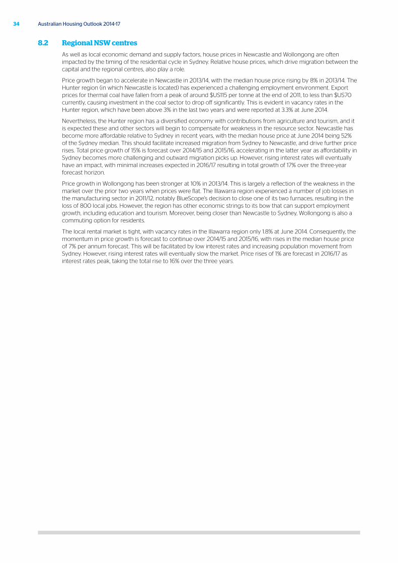
As well as local economic demand and supply factors, house prices in Newcastle and Wollongong are often impacted by the timing of the residential cycle in Sydney. Relative house prices, which drive migration between the capital and the regional centres, also play a role.
Price growth began to accelerate in Newcastle in 2013/14, with the median house price rising by 8% in 2013/14. The Hunter region (in which Newcastle is located) has experienced a challenging employment environment. Export prices for thermal coal have fallen from a peak of around $US115 per tonne at the end of 2011, to less than $US70 currently, causing investment in the coal sector to drop off significantly. This is evident in vacancy rates in the Hunter region, which have been above 3% in the last two years and were reported at 3.3% at June 2014.
Nevertheless, the Hunter region has a diversified economy with contributions from agriculture and tourism, and it is expected these and other sectors will begin to compensate for weakness in the resource sector. Newcastle has become more affordable relative to Sydney in recent years, with the median house price at June 2014 being 52% of the Sydney median. This should facilitate increased migration from Sydney to Newcastle, and drive further price rises. Total price growth of 15% is forecast over 2014/15 and 2015/16, accelerating in the latter year as affordability in Sydney becomes more challenging and outward migration picks up. However, rising interest rates will eventually have an impact, with minimal increases expected in 2016/17 resulting in total growth of 17% over the three-year forecast horizon.
Price growth in Wollongong has been stronger at 10% in 2013/14. This is largely a reflection of the weakness in the market over the prior two years when prices were flat. The Illawarra region experienced a number of job losses in the manufacturing sector in 2011/12, notably BlueScope’s decision to close one of its two furnaces, resulting in the loss of 800 local jobs. However, the region has other economic strings to its bow that can support employment growth, including education and tourism. Moreover, being closer than Newcastle to Sydney, Wollongong is also a commuting option for residents.
The local rental market is tight, with vacancy rates in the Illawarra region only 1.8% at June 2014. Consequently, the momentum in price growth is forecast to continue over 2014/15 and 2015/16, with rises in the median house price of 7% per annum forecast. This will be facilitated by low interest rates and increasing population movement from Sydney. However, rising interest rates will eventually slow the market. Price rises of 1% are forecast in 2016/17 as interest rates peak, taking the total rise to 16% over the three years.

35October 2014
Chart 19: Regional New South Wales, median house prices
-1+10
+7+7 +1
+4+8
+7+8 +1
20
40
80
160
320
640
94 95 96 97 98 99 00 01 02 03 04 05 06 07 08 09 10 11 12 13 14 15 16 17
Year ended June Source: BIS Shrapnel, ABS & REIA data
House price Wollongong ($'000)
House price Newcastle ($'000)
Forecast

36 Australian Housing Outlook 2014-17
8.3 Melbourne
After strengthening price growth of 4.8% in 2012/13, Melbourne’s median house price growth was a substantial 19.6% in 2013/14. However, it is likely this figure overstates the strength in the market; the median is also a function of the composition of sales that take place. Price growth has been strongest in inner and middle Melbourne (+12.1% and +15.8% respectively), with a more moderate increase occurring in outer Melbourne (+10.4%). A disproportionately higher volume of sales have also occurred in the high-value inner and middle suburbs, which in turn has placed the median into a higher price bracket.
Other sources that look to account for compositional changes to the sales sample, such as the ABS, suggest city-wide house price growth was still a healthy 9%–10% in 2013/14. Given the current low interest rate environment and a relatively balanced market, albeit where underlying demand has been rising, this level of growth appears to be generally in line with market conditions.
Median house price growth in Melbourne by region, per cent, 2013/14
INNER MIDDLE OUTER MEDIAN
Annual % increase 12.1 15.8 10.4 19.6
Source: Real Estate Institute of Australia
Migration has remained strong from both overseas and interstate, despite the weakness in the Victorian economy and an unemployment rate higher than the national level. This will help to support demand for housing. Further economic headwinds are expected with the manufacturing sector under pressure from a high Australian dollar. Moreover, a high level of new dwelling supply in the pipeline (mainly in the form of apartment completions) is likely to tip the market into oversupply from 2015/16, causing vacancy rates to rise.
As a result, price growth is forecast to slow considerably to 3% over 2014/15 and progressively weaken over the following two years as the excess dwelling stock expands and interest rate policy begins to tighten. With variable rates forecast to peak at 6.8% over 2016/17, this will take affordability in Melbourne close to 2008 and 2010 levels. These conditions have previously initiated a correction in prices. Consequently, a fall in house prices of 1% is forecast in 2016/17. This will take the median to $690,000 at June 2017 and result in total growth of 5% over the three-year forecast period, a 4% decline in real terms.

37October 2014
Chart 20: Melbourne dwellings, prices and activity
+2
+16 +1 -1 -4+5
+20 +3 +2-1
-1 +1 +3-7
-11
20
40
80
160
320
640
1,280
94 95 96 97 98 99 00 01 02 03 04 05 06 07 08 09 10 11 12 13 14 15 16 17
Year ended June
Real house price Melbourne ($'000)
House price Melbourne ($'000)
Commencements ('000) Victoria (Quarterly, MAT)
Average value of home loan ($'000)
Forecast
Source: BIS Shrapnel, ABS & REIA data

38 Australian Housing Outlook 2014-17
8.4 Regional Victorian centres
As well as local economic demand and supply factors, house prices in Geelong, Ballarat and Bendigo can be impacted by the timing of the residential cycle in Melbourne. New infrastructure, and the relative house prices which drive migration between the capital and regional centres, may also play a part.
All three regions are expected to benefit from the completion of the Regional Rail Link in 2014/15 which, while not necessarily resulting in a faster commute to Melbourne, should create more frequent and reliable services. The most affordable housing in Melbourne is increasingly being offered in the outer suburbs. There is the potential for some house purchasers to settle in a regional centre, where more services infrastructure may be in place and affordability and commute times are similar. These factors will potentially drive increased migration into these regional areas, creating both additional demand for dwellings and some upside to price growth.
The median house price growth experienced by Geelong was 7% in 2013/14. This level is below that of metropolitan Melbourne, although closer to that experienced by outer Melbourne. Vacancy rates were a relatively high 4.3% at June 2014, perhaps reflecting some of the economic setbacks recently experienced by the Geelong region, such as closure of the Ford engine plant and Alcoa aluminium smelter, and redundancies at Target’s head office. Nevertheless, other sectors such as education and tourism offer growth and the region is also commuting distance to Melbourne. Consequently, further price growth is expected, with Geelong’s affordability advantage over Melbourne expected to drive rises totalling 8% in the three years to 2016/17. Increases are expected to slow progressively as interest rates rise.
Median house price growth in Ballarat (+3.9%) has been below that of Geelong and Bendigo over 2013/14, which has been reflected in the weakness of new dwelling construction since 2010. With population growth on par with metropolitan Melbourne, at 2% per annum over the five years to 2013, recent vacancy rates were tight at 2.5% in June 2014. This should provide some upside to prices, which are forecast to rise by a total of 11% in the three years to 2016/17. The strongest growth will be concentrated at the start of the period when interest rates are at their lowest.
Vacancy rates in Bendigo are also relatively tight, at 2.3% in June 2014. The economic environment has been stronger, however, with the commencement of the $600 million Bendigo Hospital in 2013/14 benefiting employment levels, providing a short-term boost to house prices and the economy. Bendigo’s median house price rose by a solid 8% in 2013/14, with a relatively healthy increase of 6% forecast in 2014/15. However, price growth is then forecast to progressively slow over 2015/16 and 2016/17 as rising interest rates also have an impact. Total median house price growth over the three years to June 2017 of 10% is forecast.

39October 2014
Chart 21: Regional Victorian centres, median house prices
+1 +7+5 +3 0
+1+8
+6 +4 0
+3 +4+6
+5 0
20
40
80
160
320
640
94 95 96 97 98 99 00 01 02 03 04 05 06 07 08 09 10 11 12 13 14 15 16 17
Year ended June Source: BIS Shrapnel, ABS & REIA data
House price Bendigo ($'000)
House price Geelong ($'000)
House price Ballarat ($'000)
Forecast

40 Australian Housing Outlook 2014-17
8.5 Brisbane
After an extended period of weakness since 2010, prices in Brisbane appear to be strengthening, with growth in the median house price of 5.6% in 2013/14. However, this price growth masks a very uneven performance in the market. Median house price growth was healthy in inner (+16.8%) and middle (+8.2%) Brisbane suburbs, while the median house price declined by 1.4% in outer Brisbane.
Activity from upgraders/downsizers and investors is visible in price growth throughout the inner and middle Brisbane suburbs, although demand from these groups is still well below the previous peak in 2008. The Queensland market is estimated to be in deficiency, reflected by tight vacancy rates (2.2% in June 2014). At the current standard variable rate of 5.95%, affordability in Brisbane is at its best level since 2003.
The weakness in outer Brisbane is partly due to the fall in first home buyer demand following progressive changes to first home buyer incentives over 2012 and 2013, although there are signs in the first half of 2014 that demand is picking up. Soft state economic conditions are contributing, with the state unemployment rate of 6.6% in the three months to August 2014 exceeding the national rate of 6.1%. The population in the outer suburbs of Brisbane is also more likely to be in the employment sectors under pressure, including manufacturing, resource sector related construction and retail.
Median house price growth in Brisbane by region, per cent, 2013/14
INNER MIDDLE OUTER MEDIAN
Annual % increase 16.8 8.2 -1.4 5.6
Source: Real Estate Institute of Australia
Nevertheless, price growth is forecast to strengthen over 2014/15. Rising first home buyer demand, as well as the “ripple effect” of demand moving outwards as house prices in inner and middle Brisbane suburbs become less affordable, should contribute to positive growth in outer Brisbane. Low interest rates over the year will also assist demand.
Although declining resource sector investment will provide a drag on the State economy, many of the investment projects had a significant import component. This limited the upside impact to the state economy and will also limit the downside. Further reductions in the dollar will assist economic growth via tourism (both local and overseas) and education, while rising residential construction and potentially greater consumer spending will also contribute. As a result, slow but steady employment growth will see the unemployment rate fall.
The stock balance in Queensland will also play a part in price growth. An expected recovery in net interstate migration will match the anticipated increase in new dwelling activity, with the dwelling deficiency likely to stay relatively steady over the next three years. This will underpin stronger rises over 2014/15 (+7%) and 2015/16 (+8%), before forecast rising interest rates slow growth to 1% over 2016/17. This will take Brisbane’s median house price to a forecast $560,000 by June 2017; a rise of 17% on the June 2014 median, and a 7% increase in real terms.

41October 2014
Chart 22: Brisbane dwellings, prices and activity
+2 +3 +5 +4 -2+4+6
+7+8 +1
+3
+20+4
+6
-12
20
40
80
160
320
640
94 95 96 97 98 99 00 01 02 03 04 05 06 07 08 09 10 11 12 13 14 15 16 17
Year ended June
Real house price Brisbane ($'000)
House price Brisbane ($'000)
Commencements ('000) Queensland (Quarterly, MAT)
Average value of home loan ($'000)
Forecast
Source: BIS Shrapnel, ABS & REIA data

42 Australian Housing Outlook 2014-17
8.6 Regional Queensland centres
The regional Queensland markets of the Gold Coast, Sunshine Coast, Townsville and Cairns have all experienced generally flat prices since peaking in 2007/08. These markets were hampered by an oversupply of dwellings after the peak and generally weak local economic conditions, while other parts of regional Queensland enjoyed a boom in resource sector investment.
In the Gold Coast, the weakness in the market since 2007/08 has coincided with a severe downturn in supply. Total dwelling commencements are estimated to have declined from 7,300 in 2007/08 to a low of 2,400 in 2011/12 (–67%). As a result, rental vacancy rates have declined to a very tight 1.7% at June 2014. At June 2013 the Gold Coast’s median house price was down by 16% from its peak in real terms.
These factors coincided to drive median house price growth of 11% in 2013/14. Although new dwelling activity has been rising since the 2011/12 low, it will take some time for new stock to have a sizeable impact on the deficiency. The Gold Coast should also benefit from a pick up in the construction sector, not only the emerging recovery in residential construction, but also the expansion of the Pacific Fair shopping centre and Commonwealth Games-associated projects. As a result, further growth in the median house price of 7% is forecast in 2014/15, progressively slowing to 5% in 2015/16 and 2% in 2016/17 as forecast rises to interest rates have an impact. Total growth of 15% is forecast for the three years to 2016/17.
The Sunshine Coast is similarly undersupplied, with a vacancy rate of 1.1% reported in June 2014. After a period of weakness, the local economy is being fuelled by the commencement of the $950 million Sunshine Coast University Hospital in 2013/14 and associated works. Following a rise in the median house price of 8% in 2013/14, further healthy rises of 6% and 5% in 2014/15 and 2015/16 are forecast, slowing to 2% in 2016/17 as interest rates peak. A total rise of 14% is forecast over the period. Compared to Brisbane, population growth in both the Gold Coast and Sunshine Coast is more reliant on intra and interstate migration, which tends to increase during periods of rising prices in the eastern state capitals, which both pushes younger population into these lifestyle areas for affordability reasons, while also encouraging trade down activity from “sea changers”.
Notwithstanding flat house prices, the relatively diversified Townsville economy held up well compared to its fellow northern Queensland city of Cairns. However, conditions in the Townsville market have become more difficult in the last 12 months, with State and Federal Government fiscal consolidation impacting on administrative and defence jobs. At the same time, declining investment in the thermal coal sector has also impacted on fly-in-fly-out employment. This caused vacancy rates to rise to 5.4% by June 2014, while the median house price fell by 1% in the year. Conditions are expected to improve in line with the overall State economy, although price rises are likely to recover only slowly. Total growth of 10% is expected through to 2016/17.
In contrast, the Cairns market is now showing emerging signs of recovery. With new dwelling commencements in 2013/14 down by 73% on their 2007/08 peak, vacancy rates have tightened quickly to 2% at June 2014. This has helped to underpin growth of 10% in Cairns’ median house price. A strengthening international tourism sector and rising residential construction will help buoy the local economy and contribute to price growth. The Cairns median house price is forecast to rise by a total of 14% over the three years to 2016/17.

43October 2014
Chart 23: Regional Queensland centres, median house prices
+2+11
+7+5 +2
+3+8
+6+5 +2
-1 -1 +3 +4 +3+2+10
+5+5 +2
20
40
80
160
320
640
94 95 96 97 98 99 00 01 02 03 04 05 06 07 08 09 10 11 12 13 14 15 16 17
Year ended June Source: BIS Shrapnel, ABS & REIA data
House price Sunshine Coast
($'000)
House price Gold Coast
($'000)
House price Townsville ($'000)
Forecast
House price Cairns ($'000)

44 Australian Housing Outlook 2014-17
8.7 Adelaide
Adelaide’s median house price of $410,000 at December 2013 remained below the peak median of $410,000 at June 2010. In real terms this was a decline of 8%. Since then, there has been a pick up in price growth in Adelaide, with the median house price pushing past the $410,000 mark for the first time to be $418,200 at June 2014, representing a 5% rise for the year. Median house price growth was greatest in the inner suburbs of Adelaide (+6.7%) and weakest in outer Adelaide (1.5%).
However, the emerging recovery could be a false dawn. First home buyer activity increased ahead of the removal of the $5,000 First Home Owner’s Grant to purchasers of established dwellings after 30 June 2014. This boosted overall purchaser activity. First home buyers accounted for a disproportionately high 30% of the growth in owner occupier loans over 2013/14, which is also likely to have facilitated stronger “trade up” activity by providing demand for entry level dwellings. With future first home buyer demand having been brought forward to take advantage of the First Home Owner’s Grant before it expired, first home buyer demand is expected to weaken considerably, pressure on prices is expected to become more moderate.
Median house price growth in Adelaide by region, per cent, 2013/14
INNER MIDDLE OUTER MEDIAN
Annual % increase 6.7 5.6 1.5 4.5
Source: Real Estate Institute of Australia
Adelaide also faces headwinds in key industry sectors, with trade exposed industries, such as manufacturing, being weakened by a high Australian dollar. Automotive manufacturing will be discontinued with the closure of the Holden plant, which will impact on the businesses servicing the industry, such as automotive parts manufacture.
New dwelling activity has received a boost from the $8,500 Home Construction Grant (for all new buildings), as well as the increase in the First Home Owner’s Grant to $15,000 for purchasers of new dwellings. New dwelling commencements moved above underlying demand in 2013/14 which will result in the moderate excess expanding rather than contracting.
Nevertheless, it’s believed affordability in Adelaide is around 2002 levels and low interest rates should continue to support house price rises, albeit modest ones. Total median house price growth of 5% is forecast over the two years to 2015/16, before the combination of rising oversupply and interest rates slow price growth into 2016/17. Total price growth of 6% over the three-year forecast horizon is expected, taking the median house price to $445,000 by June 2017. This equates to a decline in real terms of 3%.

45October 2014
Chart 24: Adelaide dwellings, prices and activity
-1 +1 +0 -1 -2+1 +5 +3 +2 +1
-5
+19 +6-6 -3
5
10
20
40
80
160
320
640
94 95 96 97 98 99 00 01 02 03 04 05 06 07 08 09 10 11 12 13 14 15 16 17
Year ended June
Real house price Adelaide ($'000)
House price Adelaide ($'000)
Commencements ('000) South Australia (Quarterly, MAT)
Average value of home loan ($'000)
Forecast
Source: BIS Shrapnel, ABS & REIA data

46 Australian Housing Outlook 2014-17
8.8 Perth
An upturn emerged in the Perth market over 2012/13, with an 8% growth in the median house price. This trend was underpinned by record net overseas and interstate migration inflows, leading to tightening vacancy rates and considerable growth in rents. Demand was assisted by strong economic conditions and significantly improved affordability. In 2013/14, growth began to stall as vacancy rates rose and the economy began to slow, and an increase of 2% in the median was recorded.
Net overseas migration inflows are rapidly slowing, from 53,100 persons in 2012/13 to an estimated 37,400 in 2013/14. Across the same period, net interstate migration is likely to fall from 8,300 persons to 1,000 and eventually revert to a net outflow. This quick turnaround in population flows is likely to be one of the catalysts for the Perth vacancy rate rising to 4.2% at June 2014.
While median house price growth has been greater in inner Perth suburbs, activity has been greatest in outer Perth. This reflects the high level of first home buyer activity which, outside of the stimulus-induced levels of 2009, is at its highest level on record. The exit of first home buyers from the rental market may also be impacting on vacancy rates.
Median house price growth in Perth by region, per cent, 2013/14
INNER MIDDLE OUTER MEDIAN
Annual % increase 6.8 2.6 2.2 1.9
Source: Real Estate Institute of Australia
Although price growth has slowed, investor activity still remains solid, with the value of lending for residential investment at similar levels to the mid 2000s boom. The unemployment rate has edged upwards but remains relatively healthy at around 5% in the three months to August 2014, compared to the national figure of 6.1%.
However, the solid first home buyer and investor demand is not expected to be sufficient to drive further notable price growth. Resource sector investment has weakened and will fall considerably over the next two to three years, further impacting employment and migration. Weaker underlying demand will follow. With the current strong construction pipeline still working its way through to completion, any measured dwelling deficiency currently in the market is likely to be rapidly eroded.
As a result, the Perth residential market is forecast to weaken steadily. While low interest rates should support prices at current levels over 2014/15, and possibly 2015/16, the impact of both the slowing state economy and higher interest rates are likely to bring about price declines by 2016/17. Over the three years to June 2017, Perth’s median house price is forecast to be $525,000, or 2% below the June quarter 2014 level. In real terms, this represents a 10% decline.

47October 2014
Chart 25: Perth dwellings, prices and activity
+6 -1 -2 -3 -6
+8 +2 +1 0-3
+35
+20 -1
-15
-13
10
20
40
80
160
320
640
94 95 96 97 98 99 00 01 02 03 04 05 06 07 08 09 10 11 12 13 14 15 16 17
Year ended June
Real house price Perth ($'000)
House price Perth ($'000)
Commencements ('000) Western Australia (Quarterly, MAT)
Average value of home loan ($'000)
Forecast
Source: BIS Shrapnel, ABS & REIA data

48 Australian Housing Outlook 2014-17
8.9 Hobart
Hobart’s median house price rose by 9.4% in 2013/14 to $380,000 at June 2014. This is compared to a June quarter 2013 median of $347,300, which is likely to have understated the market given median prices in the preceding and succeeding quarters were higher. Price growth also appears to have been evenly spread across inner, middle and outer suburbs of Hobart.
The rise in the Hobart median house price in 2013/14 reflects the 23% rise in first home buyer demand over the year, and the 17% rise in lending to non-first home buyers (i.e. upgraders and downsizers). First home buyer activity has accelerated as buyers brought forward their purchase to take advantage of the $7,000 First Home Owner’s Grant before it expired on 30 June 2014. Demand for entry level properties by first home buyers helped drive an increase in demand from upgraders. However, with the grant now expired, purchaser activity is likely to slow.
Median house price growth in Hobart by region, per cent, 2013/14
INNER MIDDLE OUTER MEDIAN
Annual % increase 8.9 8.7 8.9 9.4
Source: Real Estate Institute of Australia
Despite an estimated excess dwelling stock, reflected in the vacancy rate of 3.9%, dwelling construction in Tasmania is rising. Buoyed by a $30,000 grant to first home buyers of new dwellings, the increased activity is likely to push the market further into oversupply.
The Hobart market remains very affordable at current interest rates. Tasmania’s net interstate outflow is improving from 2,600 persons in 2011/12 to an estimated 1,500 persons in 2013/14. Rising house prices in Melbourne and Sydney are likely to be encouraging some interstate migration into the more affordable Tasmanian cities. Net interstate migration is forecast to revert to balance by the end of the forecast period, or possibly sooner.
Nevertheless, the State lacks strong industry drivers to generate employment growth. With an excess dwelling stock in the market, price growth is likely to be modest and mainly underpinned by low interest rates. The median house price is forecast to rise by 1%–2% per annum, or a total 5%, to $400,000 by June 2017. This reflects a price decline of 4% in real terms, although there could be some upside to this forecast if net interstate migration strengthens more than expected.

49October 2014
Chart 26: Hobart dwellings, prices and activity
-8 +6 -0 -2 -2
-6+9 +3 +1 +1
-19 +4+8
-17-9
10
20
40
80
160
320
640
94 95 96 97 98 99 00 01 02 03 04 05 06 07 08 09 10 11 12 13 14 15 16 17
Year ended June
Real house price Hobart ($'000)
House price Hobart ($'000)
Commencements ('00) Tasmania (Quarterly, MAT)
Average value of home loan ($'000)
Forecast
Source: BIS Shrapnel, ABS & REIA data

50 Australian Housing Outlook 2014-17
8.10 Canberra
Canberra’s median house price rose above $530,000 in the first two quarters of 2014. It’s the first time the city has seen this level since peaking at $541,000 in December 2010. The median house price of $535,000 at June 2014 reflects a 5.9% rise over the previous 12 months.
This level of growth is contrary to many of the indicators in the ACT market. Record construction in recent years has resulted in an oversupply in the market, primarily in the apartment sector where building has boomed. Vacancy rates have risen to 4.2% at June 2014 and rents are declining, while the ACT now has a net interstate migration outflow after experiencing a net inflow in recent years.
The rise in the median house price appears to be a result of increased activity at the higher price points. First home buyer demand has steadily weakened over 2013/14 and lending to investors also begun to decrease in the first half of 2014. Conversely, the number of loans to non-first home buyers, who are most likely upgraders, has continued to rise through the year and is at its highest level since 2007. It appears the current low interest rate environment is driving occupiers to upgrade to a larger/higher priced home.
Median price growth in Canberra in 2013/14 has been strongest in the west and north (+10%), while in the inner and outer south price growth has been close to the Canberra median. In inner central Canberra, median prices have declined—although the relatively small volume of sales recorded in Canberra means these numbers can be quite volatile.
Median house price growth in Canberra by region, per cent, 2013/14
INNER CENTRAL INNER SOUTH WEST AND NORTH OUTER SOUTH MEDIAN
Annual % increase -4.0 4.2 10.0 5.2 5.9
Source: Real Estate Institute of Australia
The oversupply in the Canberra market is forecast to increasingly play on the residential property market over the next three years. At the same time, public sector employment is expected to continue to weaken. In the 2014 Federal Budget the Government announced a reduction in public sector employment of 16,500 persons over the following three years. As a result, vacancy rates will take some time to come down. These factors are likely to reduce the propensity for purchasers to bid up prices.
However, given the high incomes in Canberra, housing remains generally very affordable at current interest rates and there is unlikely to be too much downward pressure on prices. This should keep prices relatively flat over the next three years, with the forecast median house price of $540,000 at June 2017 only a marginal 1% up on the June 2014 median. In real terms, the Canberra median house price is forecast to decline by 8% in this period

51October 2014
Chart 27: Canberra dwellings, prices and activity
+3 +3 -4 -2 -2
+5 +6 -1 +1+1
-2 -4
-23
-19
-9
10
20
40
80
160
320
640
94 95 96 97 98 99 00 01 02 03 04 05 06 07 08 09 10 11 12 13 14 15 16 17
Year ended June
Real house price Canberra ($'000)
House price Canberra ($'000)
Commencements ('00) A.C.T. (Quarterly, MAT)
Average value of home loan ($'000)
Forecast
Source: BIS Shrapnel, ABS & REIA data
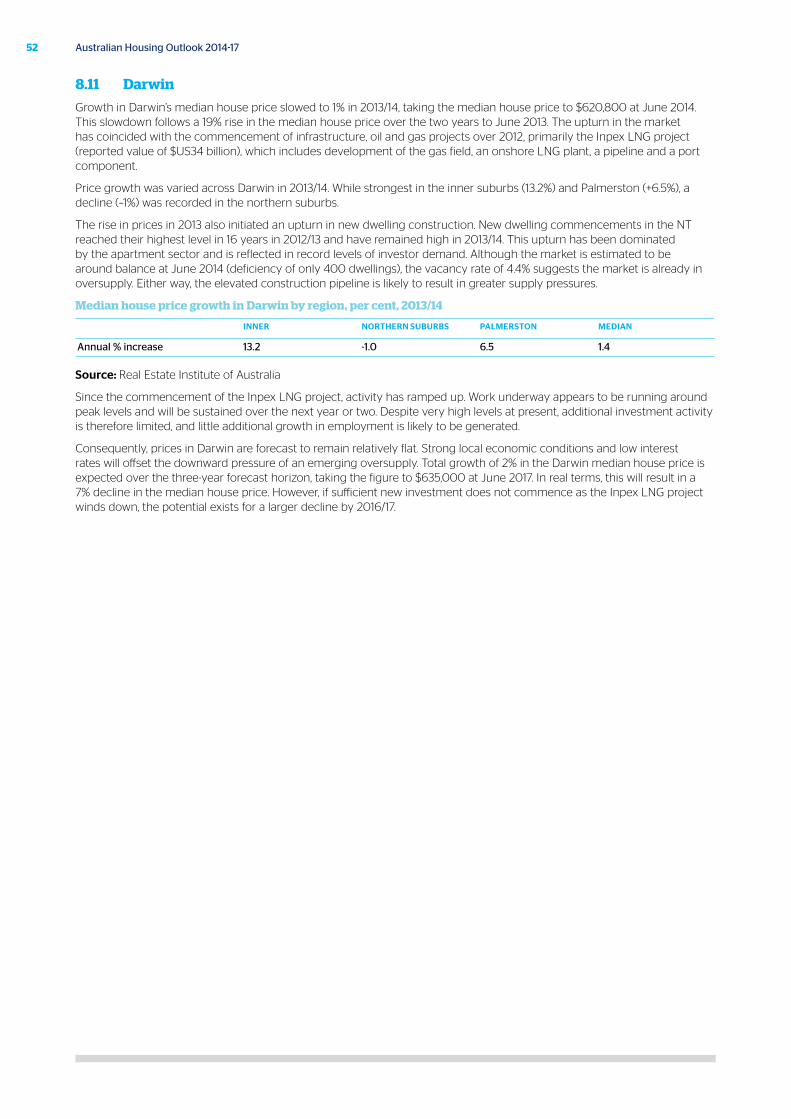
52 Australian Housing Outlook 2014-17
8.11 Darwin
Growth in Darwin’s median house price slowed to 1% in 2013/14, taking the median house price to $620,800 at June 2014. This slowdown follows a 19% rise in the median house price over the two years to June 2013. The upturn in the market has coincided with the commencement of infrastructure, oil and gas projects over 2012, primarily the Inpex LNG project (reported value of $US34 billion), which includes development of the gas field, an onshore LNG plant, a pipeline and a port component.
Price growth was varied across Darwin in 2013/14. While strongest in the inner suburbs (13.2%) and Palmerston (+6.5%), a decline (–1%) was recorded in the northern suburbs.
The rise in prices in 2013 also initiated an upturn in new dwelling construction. New dwelling commencements in the NT reached their highest level in 16 years in 2012/13 and have remained high in 2013/14. This upturn has been dominated by the apartment sector and is reflected in record levels of investor demand. Although the market is estimated to be around balance at June 2014 (deficiency of only 400 dwellings), the vacancy rate of 4.4% suggests the market is already in oversupply. Either way, the elevated construction pipeline is likely to result in greater supply pressures.
Median house price growth in Darwin by region, per cent, 2013/14
INNER NORTHERN SUBURBS PALMERSTON MEDIAN
Annual % increase 13.2 -1.0 6.5 1.4
Source: Real Estate Institute of Australia
Since the commencement of the Inpex LNG project, activity has ramped up. Work underway appears to be running around peak levels and will be sustained over the next year or two. Despite very high levels at present, additional investment activity is therefore limited, and little additional growth in employment is likely to be generated.
Consequently, prices in Darwin are forecast to remain relatively flat. Strong local economic conditions and low interest rates will offset the downward pressure of an emerging oversupply. Total growth of 2% in the Darwin median house price is expected over the three-year forecast horizon, taking the figure to $635,000 at June 2017. In real terms, this will result in a 7% decline in the median house price. However, if sufficient new investment does not commence as the Inpex LNG project winds down, the potential exists for a larger decline by 2016/17.

53October 2014
Chart 28: Darwin dwellings, prices and activity
+5-2 -1 -2
-3
+7 +1 +1 +1 0
+37
-17 0-14
-9
5
10
20
40
80
160
320
640
1,280
94 95 96 97 98 99 00 01 02 03 04 05 06 07 08 09 10 11 12 13 14 15 16 17
Year ended June
Real house price Darwin ($'000)
House price Darwin ($'000)
Commencements ('00) Northern Territory (Quarterly, MAT)
Average value of home loan ($'000)
Forecast
Source: BIS Shrapnel, ABS & REIA data

54 Australian Housing Outlook 2014-17
Median house price forecast comparison
Chart 29 shows the forecast record of the lmiHOUSING OUTLOOK™ (now known as the QBE Housing Outlook) since the inaugural 2002 report, comparing the forecast national median house price in each report over each of the three years of the forecast period with the actual movement in the national median house price. The national median is derived from a weighted median of each of our capital city forecasts.
The median house price forecasts have typically been more conservative than the actual median price rises over most three-year periods. Through the middle of the decade, the sharp rises in prices over 2007 and 2008 were not anticipated. The interest rate rises at the time were expected to have a greater dampening effect on price growth. Forecasts made over 2007 to 2009 were generally on track in terms of total growth over the three-year forecast period, despite the challenging economic conditions and negative expectations at the time that made forecasting difficult.
However, the forecasts of the national median house price in the 2010 edition of the lmiHOUSING OUTLOOK™ was more optimistic than eventual growth. The estimate of the national median house price was 12% above the June 2013 median of $520,000. Subsequent publication of Census data suggests household formation rates, and therefore underlying demand, had been lower than originally envisaged, leading to a lower dwelling deficiency in most areas and therefore less pressure on prices.
The 2011 edition forecast for 2014 was only 1% below the actual figure, while it appears the 2014 forecast in the 2012 report appears will undershoot the actual figure, after being largely on track in 2013. The forecasts published in the 2013 lmiHOUSING OUTLOOK™ have so far understated the growth that has occurred in 2014, largely due to an underestimation of the strength of the price rises in Sydney and Melbourne in the year.
Chart 29: Comparison between actual and three year forecasts, national weighted median house price
200.0
250.0
300.0
350.0
400.0
450.0
500.0
550.0
600.0
650.0
700.0
2000 2001 2002 2003 2004 2005 2006 2007 2008 2009 2010 2011 2012 2013 2014 2015 2016 2017
Actual
2002
2003
2004
2005
2006
2007
2008
2009
2010
2011
2012
2013
2014Quarter Ending June
Median House Price ($'000s)Forecast
Source: Australian Bureau of Statistics, Real Estate of Australia, Forecasts: BIS Shrapnel
9. Appendix

55October 2014
Chart 30: Comparison between actual and three year forecasts, Sydney median house price
300.0
400.0
500.0
600.0
700.0
800.0
900.0
1000.0
2000 2001 2002 2003 2004 2005 2006 2007 2008 2009 2010 2011 2012 2013 2014 2015 2016 2017
Actual
2002
2003
2004
2005
2006
2007
2008
2009
2010
2011
2012
2013
2014Quarter Ending June
Median House Price ($'000s)
Forecast
Source: Australian Bureau of Statistics, Real Estate of Australia, Forecasts: BIS Shrapnel
Chart 31: Comparison between actual and three year forecasts, Melbourne median house price
250.0
300.0
350.0
400.0
450.0
500.0
550.0
600.0
650.0
700.0
2000 2001 2002 2003 2004 2005 2006 2007 2008 2009 2010 2011 2012 2013 2014 2015 2016 2017
Actual
2002
2003
2004
2005
2006
2007
2008
2009
2010
2011
2012
2013
2014Quarter Ending June
Median House Price ($'000s)
Forecast
300.0
400.0
500.0
600.0
700.0
800.0
900.0
1000.0
2000 2001 2002 2003 2004 2005 2006 2007 2008 2009 2010 2011 2012 2013 2014 2015 2016 2017
Actual
2002
2003
2004
2005
2006
2007
2008
2009
2010
2011
2012
2013
2014Quarter Ending June
Median House Price ($'000s)
Forecast
Source: Australian Bureau of Statistics, Real Estate of Australia, Forecasts: BIS Shrapnel

56 Australian Housing Outlook 2014-17
Chart 32: Comparison between actual and three year forecasts, Brisbane median house price
150.0
200.0
250.0
300.0
350.0
400.0
450.0
500.0
550.0
2000 2001 2002 2003 2004 2005 2006 2007 2008 2009 2010 2011 2012 2013 2014 2015 2016 2017
Actual
2002
2003
2004
2005
2006
2007
2008
2009
2010
2011
2012
2013
2014Quarter Ending June
Median House Price ($'000s)Forecast
Source: Australian Bureau of Statistics, Real Estate of Australia, Forecasts: BIS Shrapnel
Chart 33: Comparison between actual and three year forecasts, Adelaide median house price
100.0
150.0
200.0
250.0
300.0
350.0
400.0
450.0
500.0
2000 2001 2002 2003 2004 2005 2006 2007 2008 2009 2010 2011 2012 2013 2014 2015 2016 2017
Actual
2002
2003
2004
2005
2006
2007
2008
2009
2010
2011
2012
2013
2014Quarter Ending June
Median House Price ($'000s)
Forecast
150.0
200.0
250.0
300.0
350.0
400.0
450.0
500.0
550.0
2000 2001 2002 2003 2004 2005 2006 2007 2008 2009 2010 2011 2012 2013 2014 2015 2016 2017
Actual
2002
2003
2004
2005
2006
2007
2008
2009
2010
2011
2012
2013
2014Quarter Ending June
Median House Price ($'000s)Forecast
Source: Australian Bureau of Statistics, Real Estate of Australia, Forecasts: BIS Shrapnel

57October 2014
Chart 34: Comparison between actual and three year forecasts, Perth median house price
150.0
200.0
250.0
300.0
350.0
400.0
450.0
500.0
550.0
600.0
650.0
2000 2001 2002 2003 2004 2005 2006 2007 2008 2009 2010 2011 2012 2013 2014 2015 2016 2017
Actual
2002
2003
2004
2005
2006
2007
2008
2009
2010
2011
2012
2013
2014Quarter Ending June
Median House Price ($'000s)
Forecast
150.0
200.0
250.0
300.0
350.0
400.0
450.0
500.0
550.0
2000 2001 2002 2003 2004 2005 2006 2007 2008 2009 2010 2011 2012 2013 2014 2015 2016 2017
Actual
2002
2003
2004
2005
2006
2007
2008
2009
2010
2011
2012
2013
2014Quarter Ending June
Median House Price ($'000s)Forecast
Source: Australian Bureau of Statistics, Real Estate of Australia, Forecasts: BIS Shrapnel
Chart 35: Comparison between actual and three year forecasts, Hobart median house price
100.0
150.0
200.0
250.0
300.0
350.0
400.0
450.0
2000 2001 2002 2003 2004 2005 2006 2007 2008 2009 2010 2011 2012 2013 2014 2015 2016 2017
Actual
2002
2003
2004
2005
2006
2007
2008
2009
2010
2011
2012
2013
2014Quarter Ending June
Median House Price ($'000s)
Forecast
100.0
150.0
200.0
250.0
300.0
350.0
400.0
450.0
500.0
2000 2001 2002 2003 2004 2005 2006 2007 2008 2009 2010 2011 2012 2013 2014 2015 2016 2017
Actual
2002
2003
2004
2005
2006
2007
2008
2009
2010
2011
2012
2013
2014Quarter Ending June
Median House Price ($'000s)
Forecast
150.0
200.0
250.0
300.0
350.0
400.0
450.0
500.0
550.0
2000 2001 2002 2003 2004 2005 2006 2007 2008 2009 2010 2011 2012 2013 2014 2015 2016 2017
Actual
2002
2003
2004
2005
2006
2007
2008
2009
2010
2011
2012
2013
2014Quarter Ending June
Median House Price ($'000s)Forecast
Source: Australian Bureau of Statistics, Real Estate of Australia, Forecasts: BIS Shrapnel

58 Australian Housing Outlook 2014-17
Chart 36: Comparison between actual and three year forecasts, Canberra median house price
150.0
200.0
250.0
300.0
350.0
400.0
450.0
500.0
550.0
600.0
2000 2001 2002 2003 2004 2005 2006 2007 2008 2009 2010 2011 2012 2013 2014 2015 2016 2017
Actual
2002
2003
2004
2005
2006
2007
2008
2009
2010
2011
2012
2013
2014Quarter Ending June
Median House Price ($'000s)Forecast
100.0
150.0
200.0
250.0
300.0
350.0
400.0
450.0
500.0
2000 2001 2002 2003 2004 2005 2006 2007 2008 2009 2010 2011 2012 2013 2014 2015 2016 2017
Actual
2002
2003
2004
2005
2006
2007
2008
2009
2010
2011
2012
2013
2014Quarter Ending June
Median House Price ($'000s)
Forecast
150.0
200.0
250.0
300.0
350.0
400.0
450.0
500.0
550.0
2000 2001 2002 2003 2004 2005 2006 2007 2008 2009 2010 2011 2012 2013 2014 2015 2016 2017
Actual
2002
2003
2004
2005
2006
2007
2008
2009
2010
2011
2012
2013
2014Quarter Ending June
Median House Price ($'000s)Forecast
Source: Australian Bureau of Statistics, Real Estate of Australia, Forecasts: BIS Shrapnel
Chart 37: Comparison between actual and three year forecasts, Darwin median house price
100.0
200.0
300.0
400.0
500.0
600.0
700.0
2000 2001 2002 2003 2004 2005 2006 2007 2008 2009 2010 2011 2012 2013 2014 2015 2016 2017
Actual
2002
2003
2004
2005
2006
2007
2008
2009
2010
2011
2012
2013
2014
Quarter Ending June
Median House Price ($'000s)Forecast
150.0
200.0
250.0
300.0
350.0
400.0
450.0
500.0
550.0
600.0
2000 2001 2002 2003 2004 2005 2006 2007 2008 2009 2010 2011 2012 2013 2014 2015 2016 2017
Actual
2002
2003
2004
2005
2006
2007
2008
2009
2010
2011
2012
2013
2014Quarter Ending June
Median House Price ($'000s)Forecast
100.0
150.0
200.0
250.0
300.0
350.0
400.0
450.0
500.0
2000 2001 2002 2003 2004 2005 2006 2007 2008 2009 2010 2011 2012 2013 2014 2015 2016 2017
Actual
2002
2003
2004
2005
2006
2007
2008
2009
2010
2011
2012
2013
2014Quarter Ending June
Median House Price ($'000s)
Forecast
150.0
200.0
250.0
300.0
350.0
400.0
450.0
500.0
550.0
2000 2001 2002 2003 2004 2005 2006 2007 2008 2009 2010 2011 2012 2013 2014 2015 2016 2017
Actual
2002
2003
2004
2005
2006
2007
2008
2009
2010
2011
2012
2013
2014Quarter Ending June
Median House Price ($'000s)Forecast
Source: Australian Bureau of Statistics, Real Estate of Australia, Forecasts: BIS Shrapnel


J5909
QBE Insurance (Australia) Limited
82 Pitt St, Sydney NSW 2000 Australia
t +61 2 9375 4444www.qbe.com.au