augmenting l1 adaptive control of piecewise constant type...

LUND UNIVERSITY

PO Box 117221 00 Lund+46 46-222 00 00

Augmenting L1 adaptive control of piecewise constant type to a fighter aircraft.Performance and robustness evaluation for rapid maneuvering

Pettersson, Anders; Åström, Karl Johan; Robertsson, Anders; Johansson, Rolf

Published in:AIAA Guidance, Navigation, and Control Conference, 13 - 16 August 2012

2012

Link to publication

Citation for published version (APA):Pettersson, A., Åström, K. J., Robertsson, A., & Johansson, R. (2012). Augmenting L1 adaptive control ofpiecewise constant type to a fighter aircraft. Performance and robustness evaluation for rapid maneuvering. InAIAA Guidance, Navigation, and Control Conference, 13 - 16 August 2012 American Institute of Aeronautics andAstronautics.

General rightsCopyright and moral rights for the publications made accessible in the public portal are retained by the authorsand/or other copyright owners and it is a condition of accessing publications that users recognise and abide by thelegal requirements associated with these rights.

• Users may download and print one copy of any publication from the public portal for the purpose of private studyor research. • You may not further distribute the material or use it for any profit-making activity or commercial gain • You may freely distribute the URL identifying the publication in the public portalTake down policyIf you believe that this document breaches copyright please contact us providing details, and we will removeaccess to the work immediately and investigate your claim.

https://portal.research.lu.se/portal/en/publications/augmenting-l1-adaptive-control-of-piecewise-constant-type-to-a-fighter-aircraft-performance-and-robustness-evaluation-for-rapid-maneuvering(f83b5f6d-d797-4ef5-8774-941efb4147cf).html

American Institute of Aeronautics and Astronautics

1

Augmenting L1 adaptive control of piecewise constant type to a fighter aircraft. Performance and robustness evaluation

for rapid maneuvering.

Anders Pettersson1 SAAB AB & Lund University, SE-58188 Linköping, Sweden

Karl J. Åström2, Anders Robertsson3, Rolf Johansson4 Lund University, SE-22100 Lund, Sweden

An L1 adaptive controller of piecewise constant type has been applied to a fighter aircraft by augmenting it to a linear state-feedback controller. Angle of attack and sideslip as well as velocity vector roll rate is demanded and controlled. It is relatively easy to design a controller augmentation this way; few parameters need to be tuned. To design an L1-controller for roll/pitch/yaw-motion of an aircraft, a five-state reference system with desired dynamics is created and three bandwidths of low-pass filters are chosen. The L1-controller activates when the aircraft aided by the feedback controller deviates from the reference dynamics. Load disturbance rejection is improved when the L1-controller is active. Results from simulations with different kinds of deviations from the nominal aircraft are presented. Special non-linear design elements need to be introduced if actuator dynamics, including rate limits, interfere with reference system dynamics. Since an L1 adaptive controller of piecewise constant type in its original form is linear time invariant, frequency domain analysis is presented, including comparisons to a typical linear state-feedback controller.

Nomenclature v = vehicle velocity vector, with vector elements u, v and w

= vehicle angular velocity vector, with vector elements p, q and r V = airspeed = angle of attack = angle of sideslip

m, Ii = mass and mass inertia F , M = force and moment acting on vehicle = density of air at the vehicle altitude

S, b, c = reference area and reference lengths, related to aerodynamic properties of the vehicle a, e, r = control surface deflections, aileron, elevator, rudder

Hm(s) = desired transfer function from plant input to output Kg = steady state inverse gain of desired transfer function from plant input to output L = state-feedback gain

I. Introduction adaptive control1 was developed with aerospace control in mind and has been found suitable for flying

vehicles in several applications2,16. Traditional adaptive schemes such as MRAC3 can give large transients and slow convergence4. In L1 adaptive control fast adaptation is achieved while robust stability to bounded plant parameter changes is claimed. Even though large adaptation gains create large and rapidly varying internal signals,

1 Systems Engineer & Doctoral Student, SAAB AB & Lund University, [email protected], AIAA Member 2 Professor Emeritus of Automatic Control, Department of Automatic Control, Lund University, [email protected] 3 Professor, Department of Automatic Control, Lund University, [email protected] 4 Professor, Department of Automatic Control, Lund University, [email protected]

L1


2

the L1 adaptive controller output is limited in amplitude and frequency, since a low-pass filter directly at the output, is used to make the controller act within the control channel bandwidth18.

There are two fundamentally different ways of controlling systems with dynamics that change over time: adaptive or robust control. The industrial baseline today is to use robust control, which caters for the effect of parametric uncertainties, although that baseline can come with an associated loss of performance. On the other hand, with an adaptive controller it is possible to boost the performance of the closed-loop system, but then the inherent robustness may be insufficient4. The ultimate goal is to address the question whether adaptive control can be used in flying vehicles that SAAB develops today or in the future.

In this application L1 adaptive controllers of piecewise constant type are applied to control a pitch-unstable fighter aircraft in angle of attack and sideslip together with angular velocity in three dimensions. Piecewise constant refers to that the controller is sampled; it internally operates in discrete time and produces parameter estimates that are piecewise constant. These controllers use the system state as controller input and can compensate for matched and unmatched disturbances1,2. Analysis and evaluation of L1-controllers are performed together with comparisons to a typical linear state-feedback control.

The main contribution of this work is use of linear system theory to the L1 adaptive controller of piecewise constant type together with a linearized fighter aircraft model. This makes it possible to analyze controller robustness in a well known framework. Frequency responses from “gang-of-six”11 transfer functions, singular value plots etc. are presented. This is done for an L1-controller and a linear state-feedback controller with integral action. Also the application of these types of controllers to a pitch-unstable fighter aircraft, including simulation results with various alterations such as parameter uncertainties and actuator failures, has a value for industries such as SAAB. Industry is also served by the insight that since L1-controllers of this type, in their original designs are linear time invariant, there are a lot of reputable methods that could end up with the same controller. It is also important to know that an L1-controller which estimates parameters and disturbances makes it possible to include non-linearities that will make the controller act on effects that can be compensated for and ignore others.

The paper is organized in the following way: Initially flight dynamics of a Gripen-like fighter are briefly derived. An L1 adaptive controller of piecewise constant type and a linear state-feedback are described and designed to the aircraft. Simulations are made in a Matlab Simulink implementation of the model. Results are presented and analyzed from a performance and robustness point of view. Linear analysis of the system in the frequency domain are presented and commented.

II. Nominal and desired dynamic motion of a flying vehicle States expressing the rigid-body-motion of a flying vehicle will be established, together with the time derivatives

of these states. This model will then be used both for deriving linear systems for design of control algorithms as well as for simulating the full environment, a well known procedure within aerospace engineering5.

A. State equation details Definitions of vectors and co-ordinates6

for creating motion equations are visualized in Figure 1. Motion around the body co-ordinate system x, y, and z-axis is defined as roll, pitch and yaw dynamics, respectively.

Expressing velocity derivatives according to Newton’s second law:

vFmv 1 and angular velocity derivatives according to the Euler equation:

)(1ii IMI

will give expressions5 in Eq. (1) for the time derivative of the system state x.

Figure 1 Body co-ordinate system xyz-axis, body velocity vector v and body angular velocity vector .

x

y z

v


3

qrIqpIprIpqIIMpqIprIqrIprIIMprIrqIpqIqrIIM

IIIIIIIII

prFFFmV

rpqFFmV

FFFm

rqp

V

x

xz2

xyyzyxz

yz22

xzxyxzy

xy22

yzxzzyx

zyzxz

yzyxy

xzxyx

zyx

zx

zyx

2

1

sincossinsincossincos1

tansincoscossincos1

cossinsincoscos1

(1)

where the velocity vector elements u, v and w are replaced by: 222 wvuV , uw /tan , 22/tan wuv . These full state equations will be used for simulations8, including non-linear aerodynamic

forces and moments depending on the missile state. When designing the controllers a linear approximation to Eq. (1) will be utilized. Using linear assumptions in

aerodynamics7 ‘Cxx’, an assumption of constant vehicle airspeed and defining dynamic pressure as 2/2Vqd , the following linearized pitch dynamics5 are achieved:

e

my

d

Nd

my

dm

y

d

Nd

Nd

epp

e

e

q

q

CIScq

CmV

Sq

qCVI

ScqC

IScq

CmV

ScqC

mVSq

Bq

Aq

2

21

2

2 (2)

The trim point5 is chosen at zero angle of attack. A pitch linear state-feedback gain (u=-Lx) will be found by solving Eq. (3) for Lp where the matrix Amp set the desired pitch dynamics:

2212

2111

lblblblb

ALBAA ppppmp (3)

After using linear approximations to Eq. (1), as was done for pitch dynamics, the following roll-yaw dynamics5 are derived:

r

a

lx

xzn

z

dl

x

xzn

z

d

Cd

Cd

nz

xzl

x

dn

z

xzl

x

d

lx

xzn

z

dl

x

xzn

z

dl

x

xzn

z

d

Cd

Cd

Cd

nz

xzl

x

dn

z

xzl

x

dn

z

xzl

x

d

r

ayy

rraa

ra

rraa

rrpp

rp

rrpp

CIIC

IScqC

IIC

ISbq

CmV

SqCmV

Sq

CIIC

ISbqC

IIC

ISbq

r

p

CIIC

VISbqC

IIC

ISbqC

IIC

VISbq

CmV

SbqCmV

SqCmV

Sbq

CIIC

VISbqC

IIC

ISbqC

IIC

VISbq

Br

pA

r

p

22

21

2

22

22

22

22

(4)

A roll-yaw linear state-feedback gain (u=-Lx) will be found by solving Eq. (5) for Ly where the matrix Amy set the desired dynamics:

yyymy LBAA (5)


4

Reference dynamics Amp and Amy are chosen based on the nominal aircraft dynamics so that desired/specified closed-loop response to demands are achieved. Eq. (3) and Eq. (5) are over-determined; a least-squares solution will produce good results. Control surfaces are manipulated by actuators which are modeled by second-order systems with rate and position limits. There is no feedback from actuator states in the control laws of this design.

III. Augmentation of an L1-controller to the system An L1 adaptive controller of piecewise constant type will be augmented (added) to the design. This is now the

plant defined by the open plant with a linear state-feedback law. The dynamics achieved by the open-loop plant controlled by the state-feedback will nominally have equal dynamics to the reference system dynamics that will be used in the L1-controller augmentation of Figure 2. In this application a piecewise constant type of L1-control is used as described in Ref. 1 Section 3.3.

Figure 2 Block diagram with reference feedforward FF, linear state-feedback L, L1-controller and Observer.

The feedforward block FF in Figure 2 creates a feedforward signals u and x using the reference r that make the plant act more linear to the controller than otherwise would be the case. In this application the feedforward will make the vehicle roll rotate around the velocity vector and compensate for mass inertia asymmetries. It will also compensate for gravity and trim the vehicle to the linearization point of Eq. (2) and Eq. (4). This will take workload off the controllers since the feedforward nominally will compensate for non-linear plant effects and bias. A state observer is used to produce estimates of plant states from measurements y. The observer also predicts state estimates forward in time (some 0.02s) to compensate for time delays in sensors models and in a simulated on-board computer.

A. Piecewise constant L1-controller design A piecewise constant L1 controller1 uses a state predictor, an adaptation law and a control law according to: State predictor

)(ˆ))(ˆ)(()(ˆ)(ˆ 21 tBttuBtxAtx ummm (6)

Adaptation law

))()(ˆ()())()(ˆ()(ˆ)(ˆ 11

2

1ss

TAsss iTxiTxeTBiTxiTxM

tt

sm )()( 1 IeAT

BBBsmTA

ms

umm (7)

Control law

)(ˆ)()()(ˆ)()()( 21

1 ssHsHssrKsCsu ummg

ummum

mmm

BAsICsHBAsICsH

1

1

)()(

)()( (8)

FF

r Plant L1

y

-L

u

-

u

x

+

+ Observer


5

System state x and state predictor x̂ are vectors of equal size. The state matrix Am sets the desired reference dynamics. A natural choice is Am = A-BmL where A is the nominal linearized plant dynamics and L corresponds to a linear state-feedback. The matrix C defines plant outputs, a linear combination of states Cxy that will be controlled to follow the equally sized, demand vector r. Bm is given by the plant input model, called the matched input matrix from control signal u which has the same size as y and r. Bum is created as the null-space of T

mB (solving the equation 0um

Tm BB ) while keeping the square matrix umm BB of full rank. This way an unmatched input

matrix Bum is created orthogonal to the direction of the matched input Bm. Time argument iTs of Eq. (7) effectuates zero order sample and hold at sampling time intervals Ts using index i, hence the name “piecewise constant”.

Hm(s) is the reference transfer function from the matched input, that is simply how the outputs are affected by the inputs. Hum(s) is the reference transfer function from unmatched inputs, which is how the outputs are affected in input directions that are orthogonal to the directions defined by Bm. This design of creating one term in the control signal u by taking the estimated unmatched error and feed it through the inverse of the matched transfer function

)(1 sH m and then the unmatched transfer function )(sHum , creates a way to compensate for unmatched disturbances. For each element in the control input u there is a matched element in ˆ , unmatched elements are added so that the size of ˆ matches the total number of states. This is not in any way unique for L1 control; the matched together with unmatched compensation could be used in other types of control designs.

The low pass filter is realized as )()()( 1 sKDsKDIsC . Bandwidth is set by KD(s) which in its simplest form is a diagonal matrix K and an integrator so D(s)=1/s. In the control law Kg is can be set to the steady state gain

11 )( mmg BCAK . This will, in steady state, couple one reference signal to one output signal by a unity gain. In this application for the pitch L1-controller, Kgp (a scalar) will be used to get correct nominal steady state gain from demanded to effectuated angle of attack. A matrix Kgy (2 by 2 elements) will be used for the roll-yaw L1-controller to cater for gains from demanded roll-rate and demanded angle of sideslip.

In Figure 3 a block diagram of a closed-loop system with an L1-controller is presented1.

Figure 3 Block diagram of system with L1-controller of piecewise constant type

For the pitch channel the L1-controller has two components in its estimate ˆ , one matched and one unmatched. The roll-yaw L1-controller is similar, the main difference being that it has three components in ˆ , two matched corresponding to the two input directions and one unmatched. Since control surface deflections in aerospace applications mainly produce moments which result in angular velocity, body rates p, q and r correspond to the matched directions. Unmatched directions correspond to angle of attack and angle of sideslip respectively.

An anti-aliasing filter where the state x enters the controller in Figure 3 should be considered. However since state measurements of x are sampled with the same or a lower frequency than the sample frequency in the L1-controller, it is assumed that the sensor has anti-aliasing filters that are tuned to the output rate. Also, it is common that the state x is estimated by an observer and then the state high-frequency content will be limited. Results presented here correspond to an implementation with estimates from a state observer.

C(s) x

ˆ

r u

Sample & Hold

x~ 1ˆ

2ˆ

-

M

BuBxAx mm ˆˆˆ

Plant

x̂ -

Kg

)()(1 sHsH umm

+

+

+


6

B. Piecewise constant L1-controller characteristics Consider the following system with non-linear state dependent input disturbances represented by matched and

unmatched functions f1 and f2:

)()(

)(,)(,)()()( 21

tCxtytxtfBtxtftuBtxAtx ummm (9)

The reference system16 used in this type of L1-control is:

)()(

)()()()()(

)(,)(,)()()(1

21

tCxty

sCxsHsrKsKDsu

txtfBtxtftuBtxAtx

refref

refmgref

refumrefrefmrefmref

111

1

)0(

)(

mmmg

mmm

BCAHK

BAsICsH (10)

The reference system will be stable if certain limits related to the norms of f1 and f2 and to the norm of KD(s) are fulfilled. It is proven in1 that if the control signal is chosen as in Eq. (6), (7) and (8), the controlled system will follow the reference system within the following limits:

)(

)(

2

1

sLref

sLref

Tuu

Txx

0)0(0)0(

2

1 (11)

The reference system follows an ideal, desired system:

)()()( srKsHsy gmid (12)

closer as the following sum of transfer function L1-norms is decreasing:

0

11)()( lsGsG

LumLm (13)

where the parameter l0 is a ratio expressing a relative maximum rate of change in f2 compared to f1 and where:

)()()()()(

)()()(1 sHCsHsCsHIsG

sCIsHsG

xummxmum

xmm

ummxum

mmxm

BAsIsH

BAsIsH

sKDsKDIsC

1

1

1

)(

)(

)()()( (14)

As the sampling period Ts goes to zero, the system in Eq. (9) will follow the reference system Eq. (10) arbitrarily closely. The reference system is unknown due to input disturbances f1 and f2, but it has a known response from these two unknown functions12,13. The functions 1 and 2 are of class , that is strictly increasing from zero1. The functions 1 and 2 become dependent on bounds on f1 and f2 and also on the L1-controller design parameters, Am, K and D(s).

This means that a reference system can be obtained that has stable but unknown responses from the reference signal r and from deviations entering via f1 and f2 to the output y. This reference system will be followed by the controlled system arbitrarily closely as gains that speed up the response to the parameter estimates are increased in the L1-controller. The reference system will follow ideal, desired system dynamics better as L1-norms (hence the name “L1”) of transfer functions Gm(s) and Gum(s) are decreased, by choosing desired dynamics set by the matrix Am and controller design parameters K and D(s).

It is an important observation that stability and performance guarantees are valid as long as the deviations fit into the f1 and f2 assumption in Eq. (9). Reducing the norms in Eq. (13) will make the robustness to deviations that do not fit into Eq. (9) smaller. As an example, a time delay does not fit into the f1 and f2 assumption at the same time as an increase of the bandwidth in C(s) reduces the norm in Eq. (13) and also reduces the time delay margin of the closed-


7

loop system. There is no known systematic way to allow a suitable portion of robustness to deviation outside f1 and f2, so manual tuning of low-pass filter parameters K and D(s) is needed.

C. Reference system dynamics design Desired dynamics for the pitch channel are set by a parameter 0p = 5 rad/s, which corresponds to closed-loop

reference response bandwidth. For the roll/yaw reference dynamics, parameters 1/ r = 6 rad/s and 0y = 4 rad/s set desired response bandwidths in this application. There are also two damping factors that place two pairs of complex-conjugated poles for the pitch and yaw channels. Both damping parameters are set to 0.9 in this design.

D. Low-pass filter bandwidth design The low-pass filters that are placed before the output of the L1-controller are first-order, discrete-time filters with

sampling period Ts in this design. Guidelines in1 for setting bandwidths in these filters are not to let frequencies beyond the control channel bandwidth18 through to the control signal.

A design is chosen which makes the unmatched low-pass parameter path having separately tuned filters from the matched, Eq. (15) and using two first-order cascaded filters. This setup was inspired by L1-controller design in14 for flying applications. Filtering the unmatched path twice will reduce high frequent noise fed through to the controller output by the unmatched parameter path. The first filter in the cascaded two-filter design uses a bandwidth that is a factor 1.2 lower than the second, also an idea from14. So in total, five low-pass filter parameters need tuning, one per state.

Low-pass filter bandwidths have been tuned the following way: simulations with random variations of vehicle parameters and characteristics have been run and evaluated for different values of low-pass filter bandwidths. Evaluation was done by calculating mean and peak deviations from desired responses in angle of attack/sideslip and roll rate together with the number of response sign shifts. Due to the fact that actuators are rate-saturated for noticeable periods in this application, generally lower values are suitable than in other L1-control applications2.

Low-pass filter bandwidths for matched pitch and yaw parameters have been related to the corresponding reference system bandwidth of section C. So diagonal values in matrix K was tuned to 2 0p for the matched pitch channel and 1.2 0y for matched yaw compensations. For roll the bandwidth 1/ r were set for matched parameter estimates. Unmatched parameter estimates, have low-pass filter bandwidths with a value of 1.2 0p and 1.8 0y for pitch and yaw respectively. These values for unmatched filters correspond to the faster of the two cascaded low-pass filters.

E. L1-controller sampling time design In a piecewise constant type of an L1-controller, the inverse of the sampling time Ts is equivalent to the adaptive

gain of a continuous time adaptive controller12. Guideline in1 for setting Ts is to choose it as low as possible, considering available computing power. In this application a sampling time of Ts=0.01 s was found suitable. A higher sampling rate than 100 Hz has not been found to add performance or robustness to the closed-loop system, grounded on simulation and linear frequency response analysis.

IV. Simulations Simulations have been carried out to display results of L1-control and state-feedback control. This is done in

order to test the controllers and system responses when different kinds of disturbance are applied.

A. Control laws to be compared To make comparisons simpler the reference signal for the L1-controller is fed directly to the aircraft actuator. It

is not passed through the low-pass filter as proposed in the original L1-controller design in1. This way the control signal for L1-control and state-feedback both uses the unfiltered term Kgr. The L1-controller augmented to a state-feedback uses the reference r and feedback from states x and estimates ˆ according to:

)(ˆ)()()()(ˆ)()()()( 21

1 ssHsHsCssCsLxsrKsu ummummg (15)

This design with an augmentation to a state-feedback is logical since the state-feedback will make the plant nominally behave like the reference system. If no state-feedback would be used and the open-loop aircraft deviates significantly from the reference system, pre-filtering of the reference r based on nominal and desired dynamics should be considered and the L1-controller would get a larger workload.


8

When the state-feedback controller is used without the augmented L1-controller, integral action is added, by use of reference systems according to mmm BAsICsH 1)()( and integrating control output error from these reference signals over time. The gain for the error integral state is chosen as the reference system steady state gain Kg. So the state-feedback controller with integral action uses the following gain from the reference r and feedback law from states x and output y:

)()()(1)()()( sysrKsHs

KsLxsrKsu gmgg (16)

Neither a gain-scheduled gain L in the state-feedback nor variable dynamics Am, Bm in the controllers were used in this controller implementation.

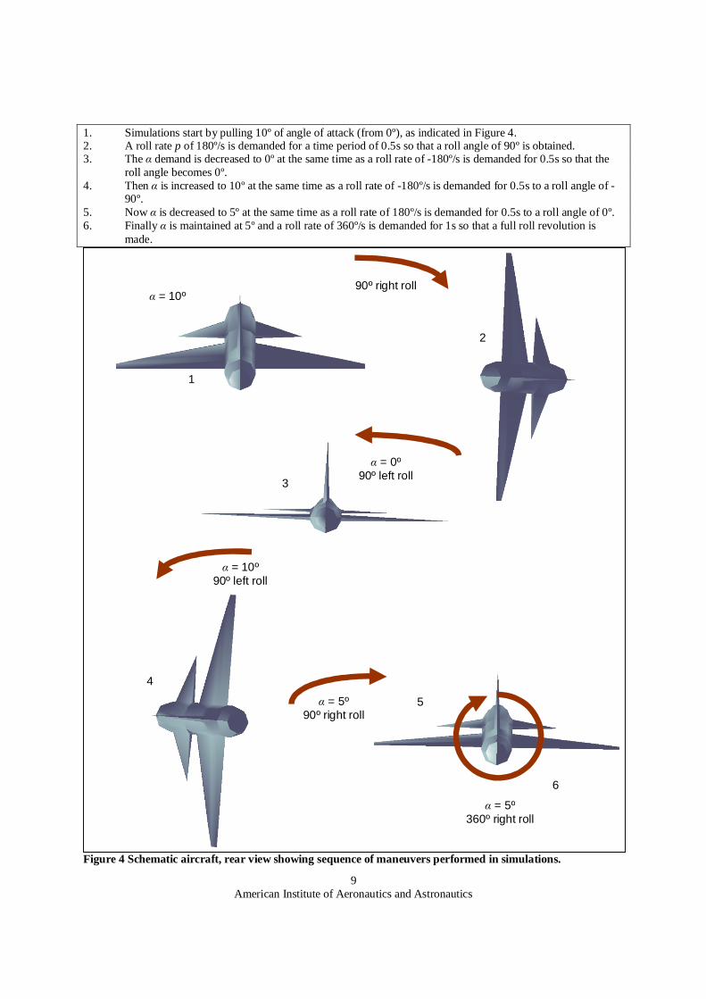
B. Scenario Demands will create changes in angle of attack and at the same time roll rotate the vehicle to different roll angles

as viewed in Figure 4. Angle of sideslip is demanded to zero throughout maneuvers. To keep and p at the demanded values while keeping small is the major task that the controller will work hard to accomplish in scenarios like these.

An altitude of about 1000m and an airspeed corresponding to M0.6 will be kept roughly constant throughout the maneuver sequence. This way changes during the simulation to dynamic pressure qd will not affect results to any large extent (however controller assumptions of altitude and airspeed are erroneous in runs with perturbations). Observed phenomena will be due to effects created by rapid maneuvering and sensor noise.


9

1. Simulations start by pulling 10º of angle of attack (from 0º), as indicated in Figure 4. 2. A roll rate p of 180º/s is demanded for a time period of 0.5s so that a roll angle of 90º is obtained. 3. The demand is decreased to 0º at the same time as a roll rate of -180º/s is demanded for 0.5s so that the

roll angle becomes 0º. 4. Then is increased to 10º at the same time as a roll rate of -180º/s is demanded for 0.5s to a roll angle of -

90º. 5. Now is decreased to 5º at the same time as a roll rate of 180º/s is demanded for 0.5s to a roll angle of 0º. 6. Finally is maintained at 5º and a roll rate of 360º/s is demanded for 1s so that a full roll revolution is

made.

Figure 4 Schematic aircraft, rear view showing sequence of maneuvers performed in simulations.

1

90º right roll

= 0º 90º left roll

2

3

4

= 10º

= 10º 90º left roll

= 5º 90º right roll

5

= 5º 360º right roll

6


10

Since roll rate demands are made open-loop with respect to achieved roll angle, they are just step functions of suitable time periods; a small roll addition is made to get roll angles that are even quarters of a turn.

C. Simulation settings and results Seven sets of parameter and noise settings in the model have been simulated: Nominal settings:

All parameters are nominal, which correspond to values that were assumed when a linearization was made to design controllers. Simulation is performed with a full 6DOF-model, including non-linear effects.

Measurement noise: Sensor noise is added to simulate a measurement procedure with sensors that produce a high level of noise. To angle of attack and angle of sideslip, normally distributed white noise with a 1 -value of 0.5° is added. To rates p, q and r normally distributed white noise with a 1 -value of 2°/s is added.

Parameter perturbations: Error in parameter assumptions are created by using normally distributed values. Pre-sampled parameter realizations are saved and used for simulations so that comparisons can be made between runs. These values are then used to perturb parameter settings relative nominal values. Start position and velocity are varied so that the 1 relative error becomes 10%. Atmospheric parameters are varied by 5%. Mass and mass inertia properties are varied by 5%. Aerodynamic parameters by 20%. Center of gravity position relative the wing cord is varied by 2% and actuator bandwidth, rate limit and damping by 10%. The parameter realization for which simulations are presented is a challenging one; it makes the needed control effort large. Feedforward compensations are still made with nominal parameter values, making this a valid check also for feedforward robustness to perturbations.

Control surface actuation failure: The right wing control surface deflection responds to an extent corresponding to half of the demand. This means that aerodynamic forces and moments created for demanded roll and pitch control surface deflection are reduced and it also creates a severe coupling between pitch and roll demands that the controller needs to compensate for, since an unforeseen right-left wing asymmetry is at hand. A challenging kind of load disturbance is created with this setup.

No feedforward applied: Feedforward signals are not added to the control signal of the plant. Controllers need to compensate for non-linear couplings without aid from feedforward based on reference signal inputs. One effect is that a demanded roll rate creates severe couplings between angle of attack and sideslip. Also effects of that the vehicle wants to rotate around its principal mass inertia axis, as well as gravity effects, will be left to controllers without aid from feedforward.

Flight at high altitude: The simulation is performed at an altitude of 7000m instead of the 1000m that controllers were designed for. Dynamic pressure will be about half of what was assumed due to lower air density. A low dynamic pressure makes the aircraft dynamics slower and the effects of control surface deflections are reduced.

No model of an actuator in L1-controller: In this setup, no actuator model is included in the state predictor of the L1-controller. There will be no knowledge in the L1-controller of actuator rate limitations.

For each of the seven different settings above, two simulations are made and presented one figure on top of the

other. One run is plotted for L1-control augmented to a state-feedback. One run is plotted for state-feedback acting on its own, including integral action.

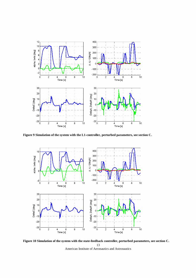
Four subplots are presented for each simulation in Figure 5 to Figure 17. Demands in angle of attack/sideslip and roll rate ( d, d and pd) are dashed lines, effectuated signals are solid lines: Subplot 1 (upper left): angle of attack (blue) and angle of sideslip (green). Subplot 2 (upper right): body rates p, q and r (blue, green and red). Subplot 3 (low left): demanded (dashed) and effectuated (solid) pitch control surface deflection e. Subplot 4 (low right): demanded and effectuated roll and yaw control demands a and r (blue and green).


11

Figure 5 Simulation of the system with the L1-controller, for nominal plant.

Figure 6 Simulation of the system with the state-feedback controller, for nominal plant.


12

Figure 7 Simulation of the system with the L1-controller, measurement noise added.

Figure 8 Simulation of the system with the state-feedback controller, measurement noise added.


13

Figure 9 Simulation of the system with the L1-controller, perturbed parameters, see section C.

Figure 10 Simulation of the system with the state-feedback controller, perturbed parameters, see section C.


14

Figure 11 Simulation of the system with the L1-controller, control surface actuation failure.

Figure 12 Simulation of the system with the state-feedback controller, control surface actuation failure.


15

Figure 13 Simulation of the system with the L1-controller, without feedforward from reference.

Figure 14 Simulation of the system with the state-feedback controller, without feedforward from reference.


16

Figure 15 Simulation of the system with the L1-controller, at a flight altitude of 7000m.

Figure 16 Simulation of the system with the state-feedback controller, at a flight altitude of 7000m.


17

Figure 17 Simulation of the system with L1-controller, no compensation of rate-limits in the L1-controller.

Figure 18 Parameter estimates 1ˆ and 2ˆ of Eq. (7) in L1-controller for case with perturbed parameters.


18

D. Comments on simulation results Overall the L1-controller augmented to a state-feedback is more robust to changes than the state-feedback with

integral action. This comes at the cost of higher noise throughput and need for special attention regarding time delay and effects of saturation.

Nominal settings Figure 5 & Figure 6: Results are similar for L1-control and state-feedback control with integral action. L1-control does a little better job at keeping and close to demanded values throughout the maneuver sequence. Peak-to-peak values for error are less than 1º throughout the simulation, a good result for both controller designs. Both controllers follow roll rate demands properly and have similar control signal amplitudes (actuator demands).

Measurement noise Figure 7 & Figure 8: Both controllers manage to keep and close to demanded values even though high noise levels were added (and the state observer was not optimized to reduce noise to the controller). L1-control is feeding more of the noise through to the control signal so that the controlled states become more excited. Peak to peak values for the pitch L1-control signal demand to elevator e was about 5º. For the state-feedback the corresponding value was about 3º. For noise to the control signal aileron a, the gain was low for both controllers. For the L1-controller this is due to that good robust performance is obtained, even though the corresponding low-pass filter had a relatively low bandwidth. For r the opposite is true, a high low-pass bandwidth is required to obtain robust performance, both in the matched and unmatched channel. This made the noise gain to r higher (peak to peak of about 8º). Overall noise levels to actuator demands are not very problematic in this application. However, the fact that the controlled state (e.g. angle of attack) is excited by sensor noise is undesired. An effort to reduce the noise by use of a tuned state observer would be necessary to increase ride quality in an aircraft application.

Parameter changes Figure 9 & Figure 10: Both controllers stabilizes the plant. The L1-controller manages to reduce effects of parameter changes to controlled states better. Other realizations of parameter values show the same thing, the L1-controller was more robust to changes than the state-feedback acting on its own. This was not accomplished with significantly higher control demands.

Control surface actuation failure Figure 11 & Figure 12: The L1-controller is less affected by this major change in matched input gains. It manages to keep , and p closer to demanded values. Control demands are not higher for the L1-controller; they are reacting faster.

No feedforward applied Figure 13 & Figure 14: Both controllers struggle to follow reference-values, large deviations occur. The L1-controller is however a bit less sensitive to this severe deviation from linear behavior in the plant dynamics.

Flight at high altitude Figure 15 & Figure 16: Demands are followed to lower degree for both controllers, the L1-controller made a little better. The performance was however not acceptable, the controllers that were designed for an altitude of 1000m can not be used for full performance missions at 7000m. This fact could be changed by Mach and altitude scheduling of the reference system, the linear state feedback and possibly the low pass filter in the L1-controller.

No model of an actuator in L1-controller Figure 17: This L1-controller design can not handle actuator rate-saturation. Without an internal model of the actuator, the controller tried to compensate for the rate-saturated actuator, which resulted in bad response and instability.

In the L1-controller an estimation of the input-load disturbance ˆ is done continuously. These matched and

unmatched parameter estimates shown in Figure 18 for the simulation in which parameters were randomly varied (corresponding to Figure 9). For pitch there are two signals, one solid for the matched load disturbance estimate and one dashed for the unmatched estimate. In roll-yaw there are two matched estimates in solid lines and one dashed unmatched estimate.

E. Estimating disturbances at different locations Special care is required if the actuator has dynamics that can not be neglected as was shown in simulations.

Estimating the disturbance at the input of the actuator would result in the controller trying to compensate for the actuator dynamics which is not possible because of actuator rate and position saturations. A better approach is presented in Figure 19 where the load disturbance is assumed to enter at the actuator output. This is the place where aerodynamic forces and moments act and also the place where control surfaces act. Therefore it is a better location for estimating and compensating input disturbances.


19

Figure 19 Block diagram of system with input disturbance estimation after actuator.

To be able to estimate a more adequate ˆ the L1-controller internal signals are interpreted physically and the state predictor is modified (the possibility is suggested in12) according to Figure 19, which is equivalent to having an actuator model including limits in rate and position at the input of the state predictor in Eq. (6). In the scenario used here, rate limits are reached frequently, position limits are seldom reached. Missiles generally have higher actuator rate limits than aircraft, even when related to the higher expected closed-loop bandwidth10, so actuator rate saturation is not as notable.

V. Frequency domain analysis of the system In the following sub-sections the L1-controller and the feedback controller, according to Eq. (15) and Eq. (16),

will be presented and commented regarding frequency characteristics, assuming that the controller and plant dynamics are linear (Eq. (2) and Eq. (4)). This will be done for the pitch channel in detail; the roll-yaw channel has similar frequency characteristics and will be included in singular value analysis. The L1-controller can be approximated by a linear time invariant system as long as the sampling time Ts is low, parameter projection bounds1 are inactive and actuator model rate/position are not saturated15. Linearized actuator dynamics and an actuator model according to Figure 19 are incorporated in this analysis. No state observer dynamics was included in this analysis, the observer that was tuned to this application only affect response at high frequencies.

A. Gang-of-Six transfer functions To investigate relevant transfer functions Figure 20 is used. Inputs are from reference r, load disturbance and

measurement noise n. Outputs are to control objective y and to control signal u.

Figure 20 Block diagram defining inputs and outputs in ”Gang-of-Six” analysis.

Controller

r

u

n

Plant y

+ +

C(s) y

ˆ

r u

- Plant

-

Actuator

Actuator model

Kg

Hm-1(s)

+

+

+


20

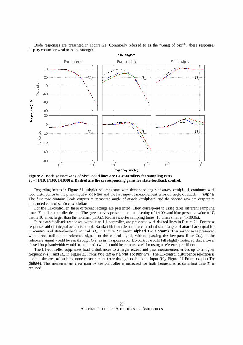
Bode responses are presented in Figure 21. Commonly referred to as the “Gang of Six”11, these responses display controller weakness and strength.

Figure 21 Bode gains ”Gang of Six”. Solid lines are L1-controllers for sampling rates Ts = [1/10, 1/100, 1/1000] s. Dashed are the corresponding gains for state-feedback control.

Regarding inputs in Figure 21, subplot columns start with demanded angle of attack r=alphad, continues with load disturbance to the plant input =ddeltae and the last input is measurement error on angle of attack n=nalpha. The first row contains Bode outputs to measured angle of attack y=alpham and the second row are outputs to demanded control surfaces u=deltae.

For the L1-controller, three different settings are presented. They correspond to using three different sampling times Ts in the controller design. The green curves present a nominal setting of 1/100s and blue present a value of Ts that is 10 times larger than the nominal (1/10s). Red are shorter sampling times, 10 times smaller (1/1000s).

Pure state-feedback responses, without an L1-controller, are presented with dashed lines in Figure 21. For these responses aid of integral action is added. Bandwidth from demand to controlled state (angle of attack) are equal for L1-control and state-feedback control (Hyr in Figure 21: From: alphad To: alpham). This response is presented with direct addition of reference signals to the control signal, without passing the low-pass filter C(s). If the reference signal would be run through C(s) as in1, responses for L1-control would fall slightly faster, so that a lower closed-loop bandwidth would be obtained. (which could be compensated for using a reference pre-filter)

The L1-controller suppresses load disturbances to a larger extent and pass measurement errors up to a higher frequency (H and Hyn in Figure 21 From: ddeltae & nalpha To: alpham). The L1-control disturbance rejection is done at the cost of pushing more measurement error through to the plant input (Hun Figure 21 From: nalpha To: deltae). This measurement error gain by the controller is increased for high frequencies as sampling time Ts is reduced.

Hyr H Hyn

Hur H Hun


21

Figure 22 Bode gains ”Gang-of-Six”. Solid lines are L1-controllers for various low-pass bandwidth parameters K = [0.1K0 , K0 , 10K0]. Dashed correspond to state-feedback control.

Figure 22 shows gains for difference low-pass settings in the L1-controller. If the bandwidth of the low-pass filters Cm(s) and Cum(s) are increased, which means that matrix K diagonal elements are increased, the input load rejection is improved (H in Figure 22), where red curves corresponds to a K ten times larger than the nominal K0 and blue curve is one tenth of the nominal. High noise gain is increased if bandwidths in low-pass filters are increased (Hyn and Hun in Figure 22), so there is a trade-off between load rejection and noise gain to be performed by choosing elements in K.

B. Open-loop controller dynamics

Open controller dynamics are presented Figure 23, corresponding to an L1-controller of Eq. (8). Responses are plotted from demanded angle of attack, alphad, from measured angle of attack, alpham, and finally from measured pitch angular rate, qm. Outputs are to demanded control surfaces deltae.

For the L1-controller, four curves are shown for different sampling times Ts. The green curves correspond to a nominal setting of 1/100s, blue present a sampling time

Hyr H Hyn

Hur H Hun

Figure 23 Bode gains for open-loop controllers. Solid lines are L1-controllers for sampling rates Ts = [1/10, 1/100, 1/1000, 1/10000] s. Dashed are the corresponding gains for state-feedback control.


22

10 times larger than the nominal (1/10s). Red and cyan present shorter sampling times of 1/1000s and 1/10000s respectively. State-feedback controller responses are dashed in Figure 23.

The augmented L1-controller path uses a higher gain from both reference signal and from measurement of the controlled state. High-frequency gains from measured angle of attack alpham for L1-control are increased as Ts is reduced. Feedback from pitch angular rate qm is reduced significantly as Ts is reduced.

This rate gain is remarkable; there will be practically no feedback from angular velocity q in the L1-controller design. If an L1-controller with unmatched compensation is implemented, this means that feedback will be done from states that are controlled, which corresponds to the signal y = Cx. So L1-methodology is stating that if there are unmatched errors, feedback should mainly use signals corresponding to the control objective. On the other hand there is derivation from alpham around 10rad/s (bode gain slope of +1), so the L1-controller is extracting pitch angular rate information from the angle of attack, instead of using rate information directly from qm. The low rate gain and alpha derivation effects are reduced if separate matched and unmatched low pass filters are tuned as in Eq. (15).

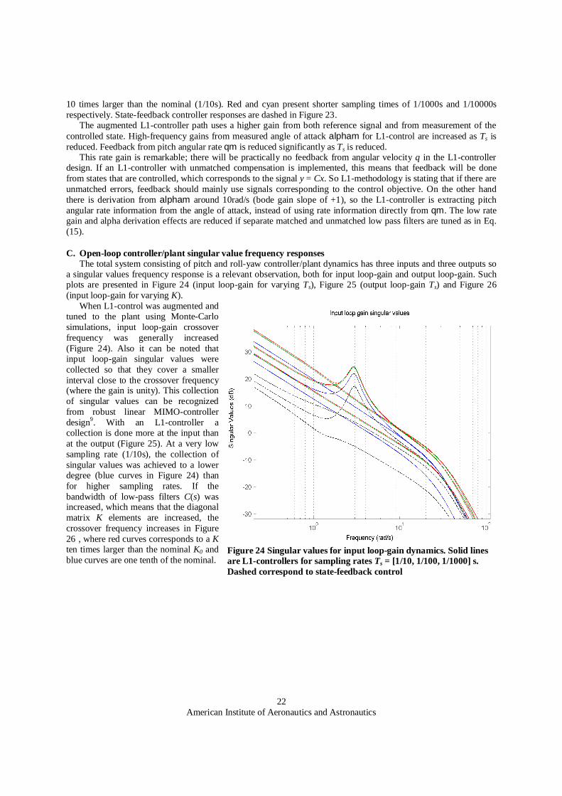
C. Open-loop controller/plant singular value frequency responses The total system consisting of pitch and roll-yaw controller/plant dynamics has three inputs and three outputs so

a singular values frequency response is a relevant observation, both for input loop-gain and output loop-gain. Such plots are presented in Figure 24 (input loop-gain for varying Ts), Figure 25 (output loop-gain Ts) and Figure 26 (input loop-gain for varying K).

When L1-control was augmented and tuned to the plant using Monte-Carlo simulations, input loop-gain crossover frequency was generally increased (Figure 24). Also it can be noted that input loop-gain singular values were collected so that they cover a smaller interval close to the crossover frequency (where the gain is unity). This collection of singular values can be recognized from robust linear MIMO-controller design9. With an L1-controller a collection is done more at the input than at the output (Figure 25). At a very low sampling rate (1/10s), the collection of singular values was achieved to a lower degree (blue curves in Figure 24) than for higher sampling rates. If the bandwidth of low-pass filters C(s) was increased, which means that the diagonal matrix K elements are increased, the crossover frequency increases in Figure 26 , where red curves corresponds to a K ten times larger than the nominal K0 and blue curves are one tenth of the nominal.

Figure 24 Singular values for input loop-gain dynamics. Solid lines are L1-controllers for sampling rates Ts = [1/10, 1/100, 1/1000] s. Dashed correspond to state-feedback control


23

D. Concluding comments on frequency responses Augmentation of an L1-controller reduces effects of input load disturbance. An L1-controller of this type that is

designed to compensate for unmatched disturbances, will feed back signals solely from the control objective (as opposed to the full state), as the adaptive gain is increased. After tuning low-pass filter parameters in the L1-controllers for this application, it can be noted that a collection of singular values were obtained for the input loop-gain frequency response at the crossover frequency. Output loop-gain singular values were not collected at the crossover frequency.

VI. Discussion Currently there is an on-going debate on the relationship among MRAC and L1 adaptive control. Robustness

issues related to the input low-pass filter of L1-controllers are controversial. In this work the focus is on application of an L1-controller to flying products. Results from linear analysis and

simulations performed in a detailed model are presented and analyzed in order to judge the suitability for aircraft and missiles. As an example, if L1-controllers should be considered as using fast adaptation or fast estimation is of less importance to industry. It is however crucial to know what to expect from L1-controllers in flying applications.

VII. Summary and conclusions An L1 adaptive controller of piecewise constant type was applied to a model of a fighter aircraft and results are

presented from an augmentation to a linear state-feedback controller. It is relatively straightforward to design an L1-controller, the desired closed-loop bandwidth is set by reference

system dynamics and then low-pass filters are tuned to balance performance and robustness. The idea of estimating input disturbances and using low-pass filtered versions of these disturbance estimates as the control signal is intuitive. In the design chosen for this application, once a five-state reference system has been chosen, five parameters for first-order low-pass filters remain to be tuned, for simultaneous roll/pitch/yaw control.

The augmentation of an L1-controller to the plant makes disturbance rejection better than for the state-feedback controller in this application. The L1-controller input disturbance estimation and compensation is suitable for flying vehicles. Forces and moments disturbing the desired vehicle motion will quickly be estimated and compensated for using counteracting control surface demands within the control channel bandwidth.

The L1-controller requires low-pass filters which have to be carefully tuned to balance performance and robustness. The final choice requires manual tuning1, systematic methods would be desirable. When a standard L1-

Figure 25 Singular values for output loop-gain dynamics. Solid lines are L1-controllers for sampling rates Ts = [1/10, 1/100, 1/1000] s. Dashed correspond to state-feedback control.

Figure 26 Singular values for input loop-gain dynamics. Solid lines are L1-controllers for low-pass bandwidth parameters K = [0.1K0 , K0 , 10K0]. Dashed correspond to state-feedback control.


24

controller is used to control a plant with long periods of rate-saturated actuators, it is hard to tune the controller. Including a model of the actuator, with rate limits, in the state predictor of the L1-controller makes tuning easier. Parameter estimates in the L1-controller can be interpreted physically since the state predictor is a model of the desired plant dynamics. Therefore it is possible to design non-linear internal models in the state predictor which will make the controller reduce effects that can be compensated for and leave other without control effort.

Compared to a state-feedback, the L1-controller augmentation increases the crossover frequency of the open-loop frequency response, thereby reducing robustness to time delays. Time delays are compensated for in this design by using prediction in a state observer. This prediction was found to be a suitable alternative to reducing bandwidths in controller low-pass filters or delaying input to the L1-controller state predictor. An L1-controller augmentation increase sensor noise gain to the control signal, in this application control signal noise levels are tolerable. Control objectives (angle of attack/sideslip) become excited by noise and since this is undesired, a state observer should be tuned to reduce this noise when used with an L1-controller.

This work used findings from2 and applied much of the same ideas. However the vehicle in this application is unstable in the pitch channel so the nominal dynamics is far from the desired, which motivates an L1-controller augmentation to a linear state feedback. It was noted in13 that L1-controllers that use output feedback are linear, here a similar discussion for full state feedback L1-controllers of piecewise constant type is made. Tuning of low-pass filter parameters was accomplished by evaluating roll/pitch/yaw channel Monte-Carlo-simulations as was done for a pitch channel implementation in14. Linear system analysis of L1-controllers was done in15 for a pitch channel; this work again does a similar thing for a roll/pitch/yaw system. In this application the actuator is rate-saturated for notable periods of time, so it was necessary to use a combination of ideas from12 and17 to be able to tune an L1-controller for this vehicle. In short; this work has used findings from previous L1-controller applications/analysis and put together a design and described results that are relevant when considering L1-control architectures for flying SAAB-products.

L1-controllers of piecewise constant type have been found to add value for control of a fighter aircraft. Augmentation to a linear state-feedback controller shows that nominal performance is maintained while improved robustness to plant perturbations is achieved. This comes at the cost of higher controller noise gain and the need for models of time delays and actuator rate-limits in the controller.

Acknowledgments This feasibility study of adaptive control for aircraft and missiles is financed by Vinnova, a Swedish

governmental agency for innovation, together with SAAB AB, a Swedish defense and security company.

References 1Hovakimyan Naira and Cao Chengyu, L1 adaptive control theory, SIAM, Philadelphia, 2010. 2Gregory I. M., Xargay E., Cao C., and Hovakimyan N., ”Flight test of L1 adaptive controller on the NASA AirSTAR flight

test vehicle”, in Proc. AIAA Guidance, Navigation and Control Conf., Toronto, AIAA-2010-8015, 2010. 3Åström K. J. and Wittenmark B., Adaptive control, Dover Publications, Inc., Mineola, 2008. 4Anderson B.D.O. and Dehghani A., ”Challenges of adaptive control – past, permanent and future”, Annual reviews in

control, 32(2) 2008 pp. 123-135. 5Nelson R. C., Flight stability and automatic control, McGraw Hill, New York, 1998. 6Stengel R. F., Flight dynamics, Princeton university press, Princeton, 2004. 7Etkin B., Dynamics of atmospheric flight, John Wiley & Sons, Inc., New York, 1972. 8Stevens B. L. and Lewis F. L., Aircraft control and simulation, John Wiley & Sons, Inc., New York, 2003. 9Bates D. and Postlethwaite I., “Robust Multivariable Control of Aerospace Systems”, DUP Science, Delft, 2002. 10Zarchan P., Tactical and strategic missile guidance, AIAA Inc., 2002. 11Åström K.J. and Hägglund T. Advanced PID Control, ISA Society, NC, 2006. 12Kharisov E., Kim K. K. K., Wang X. and Hovakimyan N., ”Limiting Behaviour of L1 Adaptive Controllers”, AIAA-2011-

6441 2011. 13van Heusden K. and Dumont G. A., “Analysis of L1 adaptive output feedback control; equivalent LTI controllers”, Sysid

2012. 14Xargai E., Hovakimyan N., Dobrokhodov V., Statnikov R.B., Kaminer I., Cao C., Gregory I. M., ”L1 Adaptive Flight

Control System Systematic Design and Verification and Validation of Control Metrics”, AIAA-2010-7773 2010. 15Seiler P., Dorobantu A and Balas G., ”Robustness Analysis of an L1 Adaptive Controller”, AIAA-2010-8407 2010. 16Hovakimyan N., Cao C, Kharisov E, Xargai E., Gregory I. M, ”L1 Adaptive Control for Safety-Critical Systems”, IEEE

Control Systems Magazine, October 2011. 17Griffin B. J., Burken J. J., Xargai E.,”L1 Adaptive Control Augmentation System with Application to X-29

Lateral/Directional Dynamics: A MIMO Approach”, AIAA GNC conference August 2010. 18Stein G., “Respect the unstable,” IEEE Control Systems Magazine, vol. 23, no. 4, Aug. 2003, pp. 12 – 25.

augmenting l1 adaptive control of piecewise constant type...

Documents