Finite Models forArithmetical Quantum Chaos

Audrey Terras

Math. Dept., U.C.S.D., San Diego, Ca 92093-0112

Abstract. Physicists have long studied spectra of Schrödinger operators andrandom matrices thanks to the implications for quantum mechanics. Analo-gously number theorists and geometers have investigated the statistics of spec-tra of Laplacians on Riemannian manifolds. This has been termed by Sarnak“arithmetic quantum chaos” when the manifolds are quotients of a symmet-ric space modulo an arithmetic group such as the modular group SL(2,Z).Equivalently one seeks the statistics of the zeros of Selberg zeta functions.Parallels with the statistics of the zeros of the Riemann zeta function havebeen evident to physicists for some time. Here we survey what may be called“finite quantum chaos” seeking connections with the continuous theory. Wewill also discuss discrete analogue of Selberg’s trace formula as well as Iharazeta functions of graphs.

Part 1

Lecture 1. Finite Models

1. Introduction

This is a story of a tree related to the spectral theory of operators on Hilbertspaces. The tree has three branches as in Figure 1. The left branch is that ofquantum physics: the statistics of energy levels of quantum mechanical systems;i.e. the eigenvalues of the Schrödinger operator Lφn = λnφn. The middle branchis that of geometry and number theory. In the middle we see the spectrum of theLaplace operator L = ∆ on a Riemannian manifold M such as the fundamentaldomain of the modular group SL(2,Z) of 2×2 integer matrices with determinant 1.This is an example of what Peter Sarnak has called “arithmetic quantum chaos.”The right branch is that of graph theory: the statistics of the spectrum of L =the adjacency operator (or combinatorial Laplacian) of a Cayley graph of a finitematrix group. We call this subject “finite quantum chaos.”

What about the roots of the tree? These roots represent zeta functions andtrace formulas. On the left is the Gutzwiller trace formula. In the middle is theSelberg trace formula and the Selberg zeta function. On the right is the Ihara zetafunction of a finite graph and discrete analogues of the Selberg trace formula. Thezeros of the zeta functions correspond sometimes mysteriously to the eigenvalues ofthe operators at the top of the tree.

Here we will emphasize the right branch and root of the tree. But we willdiscuss the connections with the other tree parts. The articles [84], [85], [86] areclosely related to these lectures. A good website for quantum chaos is that ofMatthew W. Watkins www.maths.ex.ac.uk/~mwatkins.

We quote Oriol Bohigas and Marie-Joya Gionnoni [11], p. 14: “The questionnow is to discover the stochastic laws governing sequences having very differentorigins, as illustrated in ... [Figure 2]. There are displayed six spectra, each con-taining 50 levels ...” Note that the spectra have been rescaled to the same verticalaxis from 0 to 49.

In Figure 2, column (a) represents a Poisson spectrum, meaning that of arandom variable with spacings of probability density e−x. Column (b) representsprimes between 7791097 and 7791877. Column (c) represents the resonance energiesof the compound nucleus observed in the reaction n+166Er. Column (d) comes fromeigenvalues corresponding to transverse vibrations of a membrane whose boundaryis the Sinai billiard which is a square with a circular hole cut out centered at thecenter of the square. Column (e) is from the positive imaginary parts of zero’sof the Riemann zeta function (from the 1551th to the 1600th zero). Column (f)is equally spaced - the picket fence or uniform distribution. Column (g) comesfrom Sarnak [67] and corresponds to eigenvalues of the Poincaré Laplacian on thefundamental domain of the modular group SL(2,Z) consisting of 2 × 2 integermatrices of determinant 1. From the point of view of randomness, columns (g) and(h) should be moved to lie next to column (b). Column (h) is the spectrum of afinite upper half plane graph for p=53 (a = δ = 2), without multiplicity.

Exercise 1. Produce your own versions of as many columns of Figure 2 as pos-sible. Also make a column for level spacings of lengths of primitive closed geodesicsin SL(2,Z)\H. See pages 277-280 of Terras [83], Vol. I.

Given some favorite operator L acting on some Hilbert space L2(M), as in thefirst paragraph of this section, one has favorite questions in quantum chaos theory

1. INTRODUCTION 5

Figure 1. The Tree of Quantum Chaos

(see Sarnak [67] or Hejhal et al [37] or the talks given in the spring, 1999 randommatrix theory workshop at the web site http://www.msri.org).

Examples of Questions of Interest• 1) Does the spectrum of L determine M? Can you hear the shape of M?• 2) Give bounds on the spectrum of L.• 3) Is the histogram of the spectrum of L given by the Wigner semi-circledistribution [91]?

6

Figure 2. Columns (a)-(f) are from Bohigas and Giannoni [11]and column (g) is from Sarnak [67]. Segments of “spectra,” eachcontaining 50 levels. The “arrowheads” mark the occurrence ofpairs of levels with spacings smaller than 1/4. The labels are ex-plained in the text. Column (h) contains finite upper half planegraph eigenvalues (without multiplicity) for the prime 53, withδ = a = 2 .

• 4) Arrange the spectrum of L so that λn ≤ λn+1. Consider the levelspacings |λn+1 − λn| normalized to have mean 1. What is the histogramfor the level spacings?

• 5) Behavior of the nodal lines (φn = 0) of eigenfunctions of L as n→∞.Note that when M is finite, we will consider a sequence Mj such that mj =

|Mj | → ∞ as j → ∞ and we seek limiting distributions of spectra and levelspacings as j → ∞. Now the φn = (f

(n)1 , ..., f

(n)m ) are eigenvectors of the matrix

Lj acting on the finite dimensional Hilbert space Cmj ∼= L2(Mj) and we study thelimiting behavior of the set of indices j for which f

(n)j = 0.

The trace formula is the main tool in answering such questions. We will com-pare three sorts of trace formulas in Lecture 2.

I would like to thank Stefan Erickson and Derek Newland for help with theproof reading of this article.

2. Quantum Mechanics.

Quantum mechanics says the energy levels E of a physical system are theeigenvalues of a Schrödinger equation Hφ = Eφ, where H is the Hamiltonian (adifferential operator), φ is the state function (eigenfunction of H), and E is theenergy level (eigenvalue of H). For complicated systems, physicists decided thatit would usually be impossible to know all the energy levels. So they investigatethe statistical theory of these energy levels. This sort of thing happens in ordinary

2. QUANTUM MECHANICS. 7

Figure 3. Histogram of the spectra of 200 random real 50x50symmetric matrices created using Matlab.

statistical mechanics as well. Of course symmetry groups (i.e., groups of motionscommuting with H) have a big effect on the energy levels.

In the 1950’s, Wigner (see [91]) said why not model H with a large real sym-metric n×n matrices whose entries are independent Gaussian random variables. Hefound that the histogram of the eigenvalues looks like a semi-circle (or, more pre-cisely, a semi-ellipse). For example, he considered the eigenvalues of 197 “random”real symmetric 20x20 matrices. Figure 3 below shows the results of an analogueof Wigner’s experiment using Matlab. We take 200 random real symmetric 50x50matrices with entries that are chosen according to the normal distribution. Wignernotes on p. 5: “What is distressing about this distribution is that it shows nosimilarity to the observed distribution in spectra.” However, we will find the semi-circle distribution is a very common one in number theory and graph theory. SeeFigures 7 and 9, for example. In fact, number theorists have a different name for it- the Sato-Tate distribution. It appears as the limiting distribution of the spectraof k-regular graphs as the number of vertices approaches infinity under certainhypotheses (see McKay [58]).

Exercise 2. Repeat the experiment that produced Figure 1 using uniformlydistributed matrices rather than normally distributed ones. This is a problem bestdone with Matlab which has commands rand(50) and randn(50) giving a randomand a normal random 50× 50 matrix, respectively.

So physicists have devoted more attention to histograms of level spacings ratherthan levels. This means that you arrange the energy levels (eigenvalues) Ei indecreasing order:

E1 ≥ E2 ≥ · · · ≥ En.

Assume that the eigenvalues are normalized so that the mean of the level spacings|Ei−Ei+1| is 1. Then one can ask for the shape of the histogram of the normalizedlevel spacings. There are (see Sarnak [67]) two main sorts of answers to this ques-tion: Poisson, meaning e−x, and GOE (see Mehta [59]) which is more complicated

8

Figure 4. (from Bohigas, Haq, and Pandey [12]) Level spacinghistogram for (a) 166Er and (b) a nuclear data ensemble.

to describe exactly but looks like π2xe−πx2

4 (the Wigner surmise). Wigner (see [91])conjectured in 1957 that the level spacing histogram for levels having the same val-

ues of all quantum numbers is given by π2xe−πx2

4 if the mean spacing is 1. In 1960,Gaudin and Mehta found the correct distribution function which is surprisinglyclose to Wigner’s conjecture but different. The correct graph is labeled GOE inFigure 4. Note the level repulsion indicated by the vanishing of the function at theorigin. Also in figure 4, we see the Poisson density which is e−x.

See the next section for more information on the Gaudin-Mehta distribution.You can find a Mathematica program to compute this function at the website in[30]. Sarnak [67], p. 160 says: “It is now believed that for integrable systemsthe eigenvalues follow the Poisson behavior while for chaotic systems they followthe GOE distribution.” Here GOE stands for Gaussian Orthogonal Ensemble - theeigenvalues of a random n × n symmetric real matrix as n goes to infinity. AndGUE stands for the Gaussian Unitary Ensemble (the eigenvalues of a random n×nHermitian matrix).

There are many experimental studies comparing GOE prediction and nucleardata. Work on atomic spectra and spectra of molecules also exists. In Figure 4, wereprint a figure of Bohigas, Haq, and Pandey [12] giving a comparison of histogramsof level spacings for (a) 166Er and (b) a nuclear data ensemble (or NDE) consistingof about 1700 energy levels corresponding to 36 sequences of 32 different nuclei.Bohigas et al say: “The criterion for inclusion in the NDE is that the individualsequences be in general agreement with GOE.”

More references for quantum chaos are F. Haake [33] and Z. Rudnick [65].

3. ARITHMETIC QUANTUM CHAOS. 9

3. Arithmetic Quantum Chaos.

Here we give a sketch of the subject termed “arithmetic quantum chaos”by Sarnak [67]. A more detailed treatment can be found in Katz and Sarnak[44], [45], Sarnak [67]. See Cipra [22], pp. 20-35 for a very accessible intro-duction. Another reference is the volume [37]. The MSRI website (net address:http://www.msri.org/) has movies and transparencies of many talks from 1999 onthe subject. See, for example, the talks of Sarnak from Spring, 1999. Cipra, loc.cit., p. 25 says: “Roughly speaking, quantum chaos is concerned with the spectrumof a quantum system when the classical version of the system is chaotic.” The arith-metic version of the subject involves objects of interest to number theorists whichmay or may not be known to be related to eigenvalues of operators. The first suchobjects are zeros of zeta functions. The second are eigenvalues of Laplacians onquotients of arithmetic groups.

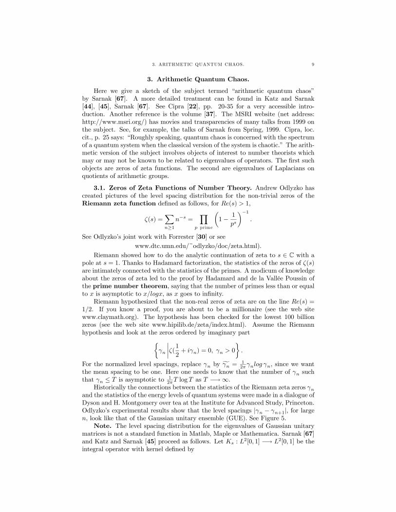
3.1. Zeros of Zeta Functions of Number Theory. Andrew Odlyzko hascreated pictures of the level spacing distribution for the non-trivial zeros of theRiemann zeta function defined as follows, for Re(s) > 1,

ζ(s) =Xn≥1

n−s =Y

p prime

µ1− 1

ps

¶−1.

See Odlyzko’s joint work with Forrester [30] or seewww.dtc.umn.edu/~odlyzko/doc/zeta.html).

Riemann showed how to do the analytic continuation of zeta to s ∈ C with apole at s = 1. Thanks to Hadamard factorization, the statistics of the zeros of ζ(s)are intimately connected with the statistics of the primes. A modicum of knowledgeabout the zeros of zeta led to the proof by Hadamard and de la Vallée Poussin ofthe prime number theorem, saying that the number of primes less than or equalto x is asymptotic to x/logx, as x goes to infinity.

Riemann hypothesized that the non-real zeros of zeta are on the line Re(s) =1/2. If you know a proof, you are about to be a millionaire (see the web sitewww.claymath.org). The hypothesis has been checked for the lowest 100 billionzeros (see the web site www.hipilib.de/zeta/index.html). Assume the Riemannhypothesis and look at the zeros ordered by imaginary part½

γn

¯ζ(1

2+ iγn) = 0, γn > 0

¾.

For the normalized level spacings, replace γn by fγn = 12πγnlog γn, since we want

the mean spacing to be one. Here one needs to know that the number of γn suchthat γn ≤ T is asymptotic to 1

2πT log T as T −→∞.Historically the connections between the statistics of the Riemann zeta zeros γn

and the statistics of the energy levels of quantum systems were made in a dialogue ofDyson and H. Montgomery over tea at the Institute for Advanced Study, Princeton.Odlyzko’s experimental results show that the level spacings |γn − γn+1|, for largen, look like that of the Gaussian unitary ensemble (GUE). See Figure 5.

Note. The level spacing distribution for the eigenvalues of Gaussian unitarymatrices is not a standard function in Matlab, Maple or Mathematica. Sarnak [67]and Katz and Sarnak [45] proceed as follows. Let Ks : L

2[0, 1] −→ L2[0, 1] be theintegral operator with kernel defined by

10

Figure 5. From Cipra [22]. Odlyzko’s comparison of level spacingof zeros of the Riemann zeta function and that for GUE (Gaussianunitary ensemble). See Odlyzko and Forrester [30]. The fit is goodfor the 1,041,000 zeros near the 2× 1020 zero.

hs(x, y) =sin

³πs(x−y)

2

´π(x−y)

2

, for s ≥ 0.

Approximations to this kernel have been investigated in connection with the un-certainty principle (see Terras [83], Vol. I, p. 51). The eigenfunctions are spher-oidal wave functions. Let E(s) be the Fredholm determinant det(I −Ks) and letp(s) = E00(s). Then p(s) ≥ 0 and R∞

0p(s)ds = 1. The Gaudin-Mehta distribution

ν is defined in the GUE case by ν(I) =RIp(s)ds. For the GOE case the kernel hs

is replaced by {hs(x, y) + hs(−x, y)}/2. See also Mehta [59].Katz and Sarnak [44], [45] have investigated many zeta and L-functions of

number theory and have found that “the distribution of the high zeroes of anyL-function follow the universal GUE Laws, while the distribution of the low-lyingzeros of certain families follow the laws dictated by symmetries associated withthe family. The function field analogues of these phenomena can be established...”More precisely, they show that “the zeta functions of almost all curves C [over afinite field Fq] satisfy the Montgomery-Odlyzko law [GUE] as q and g [the genus]go to infinity.” However, not a single example of a curve with GUE zeta zeros hasever been found.

These statistical phenomena are as yet unproved for most of the zeta functionsof number theory; e.g., Riemann’s. But the experimental evidence of Rubinstein

3. ARITHMETIC QUANTUM CHAOS. 11

[64] and Strömbergsson [79] and others is strong. Figures 3 and 4 of Katz andSarnak [45] show the level spacings for the zeros of the L-function correspond-ing to the modular form ∆ and the L-function corresponding to a certain ellipticcurve. Strömbergsson’s web site has similar pictures for L-functions correspond-ing to Maass wave forms (http://www.math.uu.se/~andreas/zeros.html). All thesepictures look GUE.

3.2. Eigenvalues of the Laplacian on Riemannian Manifolds M . Ref-erences for this subject include [16], [37], [66], [67], [83]. Suppose for concretenessthat M = Γ\H, where H denotes the Poincaré upper half plane and Γ is a dis-crete group of fractional linear transformations z −→ az+b

cz+d , for a, b, c, d real withad−bc = 1. Then one is interested in the square-integrable functions φ onM whichare eigenfunctions of the Poincaré Laplacian; i.e.,

(3.1) ∆φ = y2µ∂2φ

∂x2+

∂2φ

∂y2

¶= λφ.

The most familiar example of an arithmetic group is SL(2,Z), themodular groupof 2 × 2 integer matrices of determinant one. A function φ which is Γ-invariant,satisfies (3.1), and is square integrable on M is a Maass cusp form. The λ0sform the discrete spectrum of ∆. Studies have been made of level spacings of theeigenvalues λ. The zeta function that is involved is the Selberg zeta function (definedin Table 3 of Lecture 2). Its non-trivial zeros correspond to these eigenvalues.

Because M is not compact for the modular group, there is also a continuousspectrum (the Eisenstein series). This makes it far more difficult to do numericalcomputations of the discrete spectrum. See Terras [83], Vol. I, p. 224, for somehistory of early numerical blunders. Other references are Elstrodt [25] and Hejhal[36]. Equivalently one can replace the Poincaré upper half plane with the Poincaréunit disk.

I like to say that an arithmetic group is one in which the integers are lurkingaround in its definition. Perhaps a number theorist ought to be able to smell them.

If you really must be precise about it, you should look at the articles of Borel[14], p. 20. First you need to know that 2 subgroups A,B of a group C are said tobe commensurable iff A∩B has finite index in both A and B. Then suppose Γ isa subgroup an algebraic group G over the rationals as in Borel [14], p. 3. One saysthat Γ is arithmetic if there is a faithful rational representation (see Borel [14],p. 6) ρ : G→ GL(n), the general linear group of n×n non-singular matrices, suchthat ρ is defined over Q and such that ρ(Γ) is commensurable with ρ(Γ)∩GL(n,Z).Arithmetic and non-arithmetic subgroups of SL(2,C) are discussed by Elstrodt,Grunewald, and Mennicke in [26], Chapter 10.

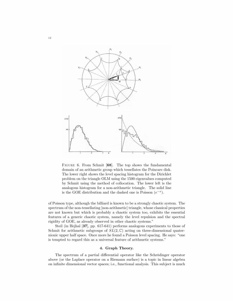
The top of Figure 6 shows the fundamental domain of an arithmetic group inthe unit disk. Note that the upper half plane can be identified with the unit discvia the map sending z in H to z−i

z+i . C. Schmit [68] found 1500 eigenvalues forthe Dirichlet problem of the Poincaré Laplacian on the triangle OLM with anglesπ/8, π/2, π/3. The histogram of level spacings for this problem is the lower rightpart of Figure 6. Schmit also considered the Dirichlet problem for a non-arithmetictriangle with angles π/8, π/2, 67π/200. The level spacing histogram for this non-arithmetic triangle is given in the lower left of Figure 6. Schmit concludes: “Thespectrum of the tessellating [arithmetic] triangle exhibits neither level repulsion norspectral rigidity and there are strong evidences that asymptotically the spectrum is

12

Figure 6. From Schmit [68]. The top shows the fundamentaldomain of an arithmetic group which tessellates the Poincare disk.The lower right shows the level spacing histogram for the Dirichletproblem on the triangle OLM using the 1500 eigenvalues computedby Schmit using the method of collocation. The lower left is theanalogous histogram for a non-arithmetic triangle. The solid lineis the GOE distribution and the dashed one is Poisson (e−x).

of Poisson type, although the billiard is known to be a strongly chaotic system. Thespectrum of the non-tessellating [non-arithmetic] triangle, whose classical propertiesare not known but which is probably a chaotic system too, exhibits the essentialfeatures of a generic chaotic system, namely the level repulsion and the spectralrigidity of GOE, as already observed in other chaotic systems.”

Steil (in Hejhal [37], pp. 617-641) performs analogous experiments to those ofSchmit for arithmetic subgroups of SL(2,C) acting on three-dimensional quater-nionic upper half space. Once more he found a Poisson level spacing. He says: “oneis tempted to regard this as a universal feature of arithmetic systems.”

4. Graph Theory.

The spectrum of a partial differential operator like the Schrödinger operatorabove (or the Laplace operator on a Riemann surface) is a topic in linear algebraon infinite dimensional vector spaces; i.e., functional analysis. This subject is much

4. GRAPH THEORY. 13

harder than the finite dimensional version. So, like S. Wolfram with his cellularautomata, let us replace the continuous, calculus-oriented subject, with a finitecomputer-friendly subject. It is clearly much easier to experiment with the finitequantum chaos statistics. One does not need a supercomputer!

So we replace the differential operator with a finite analogue - the adjacencymatrix/operator of a graph. Think of a graph as a system of masses connected bysprings or rubber bands. This is a reasonable model for a molecule. See Starzak[77]. Here we consider only Cayley graphs of groups for which we understand therepresentations. This will be a big help in computing the eigenvalues/energy levelssince by a result in the first chapter or so of a book on group representations, theadjacency operation of a Cayley graph of a group G is block diagonalized by theFourier transform on G. See [82], pp. 256-7, 284.

The spectral theory of graphs has a long history in its own right. See Biggs [10]and Cvetkovic, Doob and Sachs [23] as well as the more recent book of Fan Chung[20]. Much of the motivation comes from quantum chemistry as well as physics,mechanical engineering, and computer science. One would also expect that thereshould be more applications in areas such as numerical analysis for problems withsymmetry. Hückel’s theory in chemistry seeks to study such things as the stabilityof a molecule by computing a constant from the eigenvalues of A for the graphassociated to the molecule. One very interesting example was provided recentlyby the work of Chung and Sternberg [21] on the application of the representationtheory of the icosahedral group to explain the spectral lines of the buckyball C60.They find that the stability constant for the buckyball is greater than that forbenzene. See also Chung [20] and Sternberg [78].

Most of spectral graph theory is not really concerned with finding histogramssuch as Figures 7 and 8, but instead with more basic questions such as 2b) below.I will assume that our graph X is connected finite and k-regular with adjacencymatrix A. Here "k-regular" means that each vertex has k edges coming out.

Now we can re-interpret the 5 questions at the end of section 1 when M is afinite connected regular graph. As we said, for most questions below, we will needan infinite sequence of graphs Xj with |Xj | → ∞, as j → ∞. We assume Xj hasadjacency matrix Aj . In question 2b) a graph X is "bipartite" if X = A∪B, whereA ∩B = ∅ such that any edge connects a vertex in A to a vertex in B.

Basic Questions about Spectra of Finite Connected k-Regular Graphs• 1) Can non-isomorphic graphs have the same spectrum? Can you hearthe shape of a graph?

• 2) a) What are bounds on the spectrum of A? Note that k is always aneigenvalue of multiplicity 1. And −k is an eigenvalue iff X is bipartite.Are there gaps in the spectrum or does it approach the interval [−k, k] asthe number of vertices of the graph goes to infinity? Is 0 an eigenvalue ofA?

b) What does the size of the second largest eigenvalue of A in absolutevalue have to do with graph-theoretic constants such as diameter, girth,chromatic number, expansion constants?

• 3) Does the histogram of the spectrum of Aj (the adjacency matrix of Xj)approach the Wigner semi-circle distribution for a sequence of graphs Xj ,with |Xj |→∞, as j →∞?

14

• 4) Arrange the spectrum {λn}of Aj so that λn ≤ λn+1. Consider the levelspacings |λn+1 − λn| normalized to have mean 1. What is the limitinghistogram for the level spacings as j →∞?

• 5) What can be said about the behavior of the eigenfunctions (eigenvec-tors) of A?

Here we will discuss some of these questions for some special types of graphs.

Exercise 3. Show that for a connected k-regular graph X, the degree k isalways an eigenvalue of multiplicity 1. Prove that −k is an eigenvalue iff X isbipartite. Figure out the definitions of diameter, girth, chromatic number, expansionconstant of a graph and explore the connections with bounds on the second largesteigenvalue of A in absolute value. References are: Biggs [10] , Bollobas [13],Terras [82].

It was shown by Alon and Boppana (see Lubotzky [52], p. 57 or Feng and Li[28] for a generalization to hypergraphs) that for connected k-regular graphs X, ifλ(X) denotes the second largest eigenvalue of A in absolute value, then

lim inf λ(X) ≥ 2(k − 1)1/2, as |X| −→∞.

Following Lubotzky, Phillips and Sarnak [53], we call a k-regular graph X Ra-manujan iff

(4.1) λ(X) ≤ 2(k − 1)1/2.Thus Ramanujan graphs are the connected k-regular graphs with the smallest pos-sible asymptotic bound on their eigenvalues. Such graphs are good expanders and(when the graph is not bipartite) the standard random walk on X converges ex-tremely rapidly to uniform. This means that Ramanujan graphs make efficientcommunications networks. See Lubotzky [52], Sarnak [66], and Terras [82]. Fi-nally Ramanujan graphs are those for which the Ihara zeta function satisfies theanalogue of the Riemann hypothesis. See Exercise 9 in Lecture 2.

Remark 1. The name “Ramanujan” was attached to these graphs by Lubotzky,Phillips and Sarnak [53] because they needed to use the (now proved) Ramanujanconjecture on the size of Fourier coefficients of modular forms such as ∆ in orderto show that the graphs they created did satisfy the inequality (4.1).

Margulis as well as Lubotzky, Phillips and Sarnak [53] construct examples ofinfinite families of Ramanujan graphs of fixed degree. See also Morgenstern [61].There are also examples such as the graphs of Winnie Li [49] and the Euclideanand finite upper half plane graphs in Terras [81] and [82] (see the discussion ofFigures 7, 8 and 9 below) which are Ramanujan but the degree increases as thenumber of vertices increases. Jakobson et al (in [37], pages 317-327) studied theeigenvalues of adjacency matrices of generic k-regular graphs and found the levelspacing distribution looks GOE as the number of vertices goes to infinity. Theirresults are purely experimental.

Since Lubotzky, Phillips and Sarnak [53] or even earlier, it has been of interestto look at Cayley graphs associated with groups like GL(2, F ), the general lineargroup of 2 × 2 invertible matrices with entries in F , where F is a finite field orring. Subgroups like SL(2, F ), the special linear group of determinant 1 matrices inGL(2, F ), are also important. These groups are useful thanks to the connection with

4. GRAPH THEORY. 15

modular forms - making it possible to use some highly non-trivial number theoryto prove that the graphs of interest are Ramanujan, for example. See Lubotzky[52] and Sarnak [66]. Other references are Chung [20], Friedman [31], and Li [49].

A Cayley graph of a finite group G with edge set S ⊂ G will be denotedX = X(G,S). X has as vertex set the elements of G and edges connect x ∈ G toxs for all s ∈ S. Normally we assume that S is "symmetric" meaning that s ∈ Simplies s−1 ∈ S. This allows us to consider X to be an undirected graph. If Sgenerates G then X is connected. Usually we assume the identity element of G isnot in S so that X will not have loops.

If G is the cyclic group Z/nZ, it is easy to see that a complete orthogonal set ofeigenfunctions of A are the characters of G. The characters are χa(x) = e2πiax/n,for a ∈ Z/nZ. The corresponding eigenvalues are λa =

Xs∈S

χa(s). The same formula

works for any finite abelian group. When the group is not abelian, things becomemore complicated. See Terras [82].

Histograms of spectra or of level spacings were not considered until later, butLafferty and Rockmore [48] (and in [31], pp. 63-73) consider spectral plots thatshow spectral gaps. In [37], pp. 373-386, Lafferty and Rockmore investigate levelspacing histograms. They found on page 379, for example, that the cumulativedistribution for the level spacings of ten 4-regular graphs on 2,000 vertices generatedby running a Markov chain for 108 steps looks remarkably close to the cumulative

distribution function for the Wigner surmise 1− exp³−πx24

´. And in Lafferty and

Rockmore in [37], p. 380, they found that the cumulative distribution functionfor eigenvalue spacings of the Cayley Graph X(SL(2,Z/157Z), {t, t−1, w,w−1}),excluding the first and second largest eigenvalues, setting

t =

µ14 144101 153

¶and w =

µ114 129140 124

¶,

looks extremely close to the Poisson cumulative distribution 1− e−x.

4.1. Finite Euclidean Space. Along with some colleagues at U.C.S.D. wehave looked at histograms of various Cayley graphs. Some of this is discussed inmore detail in my book [82]. In the following discussion p is always an odd primeto make life simpler. We begin with finite analogues of Euclidean space.

We want to replace real symmetric spaces such as the plane R2 with finiteanalogues like F2p, where Fp denotes the field with p elements. We can define a

finite “distance” on vectors x =µ

x1x2

¶∈ F2p by

(4.2) d(x, y) = (x1 − y1)2 + (x2 − y2)

2.

This distance is not a metric but it is invariant under translation and a finiteanalogue of rotation and thus under a finite analogue of the Euclidean motiongroup.

Define the finite Euclidean plane graph to be the Cayley graph X(F2p, S),where S = S(a, p) consists of solutions x = (x1, x2) ∈ F2p of the congruence

x21 + x22 ≡ a (modp).

16

The points in S form a finite circle. It turns out (Exercise 4) that the eigenvaluesof the adjacency matrices for these graphs are essentially Kloosterman sums, forcolumn vectors b ∈ F2p :

(4.3) λb =Xx∈S

e2πitbx/p.

Here tb =transpose of b and thus tbx = b1x1 + b2x2. Kloosterman sums are finiteanalogues of Bessel functions just as Gauss sums are finite analogues of gammafunctions. See Terras [82]. pp. 76, 90.

Exercise 4. Prove that for odd primes p the eigenvalues in (4.3) are given by

λ2c =G21pK(a, d(c, 0)),

where d(x, y) is as in (4.2), G1 is the Gauss sum

G1 =

p−1Xt=0

ε(t)e2πit/p,

with ε(t) =³tp

´= the Legendre symbol; i.e.,

ε(t) =

0, if p divides t1, if t is a square mod p−1, otherwise.

Finally the Kloosterman sum is

(4.4) K(a, b) =

p−1Xt=1

exp

µ2πi(at+ b/t)

p

¶.

See p. 95 of my book [82] for hints.

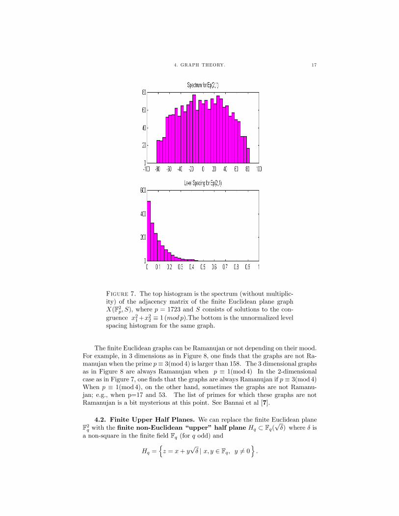
André Weil ([90], Vol. I, pp. 386-9) estimated the Kloosterman sum (4.4)which implies that the finite Euclidean graphs are Ramanujan when p ≡ 3(mod 4).In the case p ≡ 1(mod 4), the graphs may fail to be exactly Ramanujan but they areasymptotically Ramanujan as p −→∞. Katz [43] has proved that the distributionof the Kloosterman sums becomes semi-circle in the limit for large p. The top partof Figure 7 gives the histogram for the spectrum of one of the finite Euclidean planegraphs. The bottom part of Figure 7 gives the level spacing for the same Cayleygraph, which does indeed look to be Poisson.

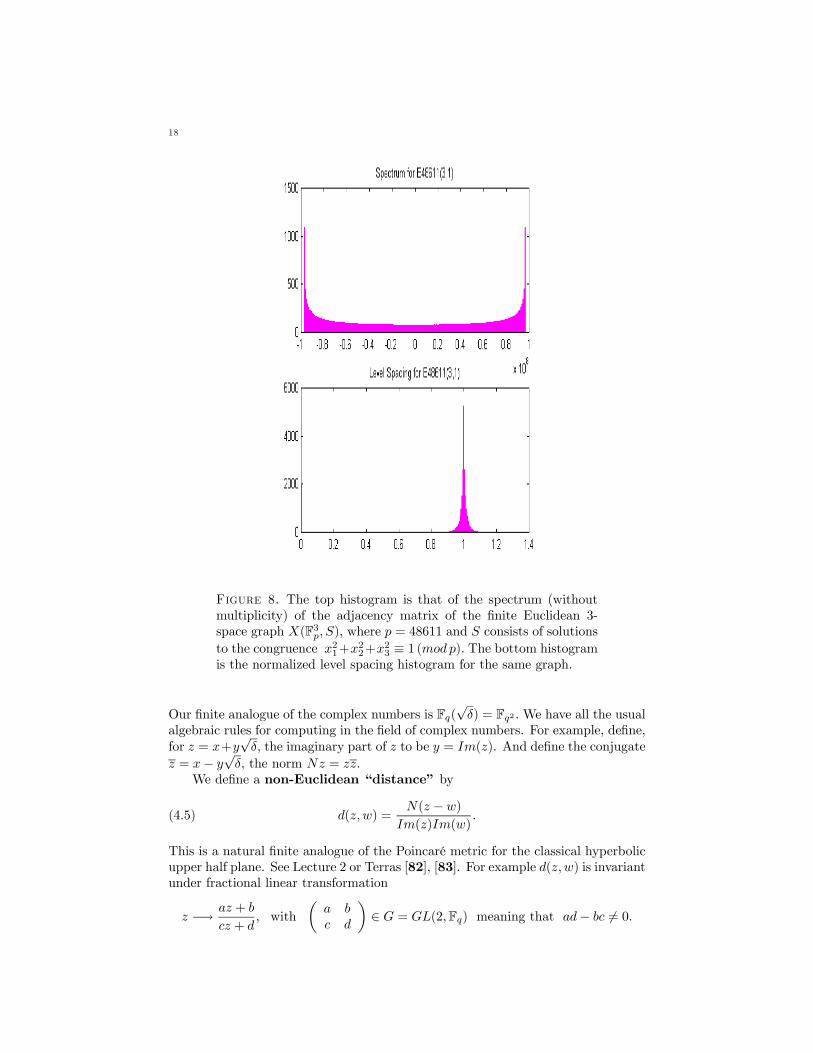
However when one replaces the 2-dimensional Euclidean graphs with three-dimensional analogues, the Kloosterman sums can be evaluated as sines or cosines.If we throw out the half of the eigenvalues of E48611(3, 1) that are 0, we obtain thehistogram in the top of Figure 8 which is definitely not the semi-circle distribution.If we had kept the 0 eigenvalues, there would also be a peak at the origin. Thenormalized level spacing histogram for E48611(3, 1) is in the bottom of Figure 8.And the bottom does not appear to be Poisson either. See Terras [82] for moreinformation. Bannai et al [7] have generalized these Euclidean graphs to associationschemes for finite orthogonal groups.

4. GRAPH THEORY. 17

Figure 7. The top histogram is the spectrum (without multiplic-ity) of the adjacency matrix of the finite Euclidean plane graphX(F2p, S), where p = 1723 and S consists of solutions to the con-gruence x21+x22 ≡ 1 (modp).The bottom is the unnormalized levelspacing histogram for the same graph.

The finite Euclidean graphs can be Ramanujan or not depending on their mood.For example, in 3 dimensions as in Figure 8, one finds that the graphs are not Ra-manujan when the prime p≡ 3(mod 4) is larger than 158. The 3 dimensional graphsas in Figure 8 are always Ramanujan when p ≡ 1(mod 4) In the 2-dimensionalcase as in Figure 7, one finds that the graphs are always Ramanujan if p ≡ 3(mod 4)When p ≡ 1(mod 4), on the other hand, sometimes the graphs are not Ramanu-jan; e.g., when p=17 and 53. The list of primes for which these graphs are notRamanujan is a bit mysterious at this point. See Bannai et al [7].

4.2. Finite Upper Half Planes. We can replace the finite Euclidean planeF2q with the finite non-Euclidean “upper” half plane Hq ⊂ Fq(

√δ) where δ is

a non-square in the finite field Fq (for q odd) and

Hq =nz = x+ y

√δ | x, y ∈ Fq, y 6= 0

o.

18

Figure 8. The top histogram is that of the spectrum (withoutmultiplicity) of the adjacency matrix of the finite Euclidean 3-space graph X(F3p, S), where p = 48611 and S consists of solutionsto the congruence x21+x

22+x

23 ≡ 1 (mod p). The bottom histogram

is the normalized level spacing histogram for the same graph.

Our finite analogue of the complex numbers is Fq(√δ) = Fq2 .We have all the usual

algebraic rules for computing in the field of complex numbers. For example, define,for z = x+y

√δ, the imaginary part of z to be y = Im(z). And define the conjugate

z = x− y√δ, the norm Nz = zz.

We define a non-Euclidean “distance” by

(4.5) d(z, w) =N(z − w)

Im(z)Im(w).

This is a natural finite analogue of the Poincaré metric for the classical hyperbolicupper half plane. See Lecture 2 or Terras [82], [83]. For example d(z,w) is invariantunder fractional linear transformation

z −→ az + b

cz + d, with

µa bc d

¶∈ G = GL(2,Fq) meaning that ad− bc 6= 0.

4. GRAPH THEORY. 19

Fix an element a ∈ Fq with a 6= 0, 4δ. Define the vertices of the finite upperhalf plane graph Pq(δ, a) to be the elements of Hq. Connect vertex z to vertexw iff d(z,w) = a. See the Figure 14 in Lecture 2 for examples of such graphs.

Exercise 5. Show that the octahedron is the finite upper half plane graphP3(−1, 1).

It turns out (see Terras [82]) that simultaneous eigenfunctions for the adjacencymatrices of these graphs, for fixed δ as a varies over Fq, are spherical functions forthe symmetric space G/K, where K is the subgroup fixing

√δ. Thus K is a finite

analogue of the group of real rotation matrices O(2,R). We will say more aboutsymmetric spaces in the last section of this set of lectures. In particular, see Table2 in Lecture 2 for a comparison of spherical functions on our 3 favorite symmetricspaces.

A spherical function (see [82], Chapter 20) h : G −→ C is defined to bea K bi-invariant eigenfunction of all the convolution operators by K- bi-invariantfunctions; it is normalized to have the value 1 at the identity. Here K- bi-invariantmeans f(kxh) = f(x), for all k, h ∈ K,x ∈ G and convolution means f ∗h, where(4.6) (f ∗ h) (x) =

Xy∈G

f(y)h(y−1x).

These are generalizations of Laplace spherical harmonics (see Terras [83], Vol.I, Chapter 2). Equivalently h is a spherical function means h is an eigenfunctionfor the adjacency matrices of all the graphs Pq(δ, a), as a varies over Fq. One canshow ([82], p. 347) that any spherical function has the form

(4.7) h(x) =1

|K|Xk∈K

χ(kx), where χ is a character of G = GL(2,Fq).

Here χ is an irreducible character appearing in the induced representation of thetrivial representation of K induced up to G. In this situation (when G/K is asymmetric space or (G,K) a Gelfand pair) eigenvalues = eigenfunctions. SeeStanton [72] and Terras [82], p. 344. Thus our eigenvalues are finite analogues ofLegendre polynomials.

One can also view the eigenvalues of the finite upper half plane graphs as entriesin the character table of an association scheme. See Bannai [6]. And this wholesubject can be reinterpreted in the language of Hecke algebras. See Krieg [47].

Soto-Andrade [71] managed to rewrite the sum (4.7) for the case G/K ∼= Hq

as an explicit exponential sum which is easy to compute (see [82], p. 355 and Ch.21). Thus we can call the eigenvalues of the finite upper half plane graphs Soto-Andrade sums. Katz [42] estimated these sums to show that the finite upper halfplane graphs are indeed Ramanujan. Winnie Li [49] gives a different proof.

The spectral histograms for the finite upper half plane graphs for fairly large qlook like Figure 9. The spectra appear to resemble the semi-circle distribution andthe level spacings appear to be Poisson. Recently Ching-Li Chai and Wen-ChingWinnie Li [18] have proved that the spectra of finite upper half plane graphs doapproach the semi-circle distribution as q goes to infinity. They use the Jacquet-Langlands correspondence for GL(2) over function fields and the connection WinnieLi has made between the finite upper half plane graphs and Morgenstern’s functionfield analogues (see [61]) of the Lubotzky, Phillips and Sarnak graphs. See Li’sarticle in [37] pp. 387-403. Note that the result of Chai and Li does not follow

20

from the work of McKay [58] because the degrees of the finite upper half planegraphs approach infinity with q. The Poisson behavior of the level spacings forfinite upper half planes is still only conjectural.

However if you replace the finite field Fq with a finite ring like Z/qZ, for q =pr, p =prime, r > 1, the spectral histograms change to those in Figure 10 whichdo not resemble the semi-circle at all.

Here we view finite upper half planes as providing a "toy" symmetric space.But an application has been found (see Tiu and Wallace [88] ).

Figure 9. Histograms of Spectra of Finite Upper Half PlaneGraphs (without multiplicity) P353(3, 3). In our program to com-pute Soto-Andrade sums we needed to know that a generator of themultiplicative group of F353(

√3) is 1 + 5

√3. The top histogram

is for the spectrum and the lower one is for the unnormalized levelspacing.

Exercise 6. Define finite upper half plane graphs over the finite fields of char-acteristic 2. The spectra of these graphs have been considered in Angel [3] andEvans [27]. Using a result of Katz, the non-trivial graphs have also been proved tobe Ramanujan.

4. GRAPH THEORY. 21

Figure 10. Histograms of Spectra (without multiplicity) of FiniteUpper Half Plane Graphs over the Ring Z/169Z with d = 2 anda = 17. The top histogram is that for the spectrum and the bottomone is that for the unnormalized level spacing. Data was computedby B. Shook using Matlab. See Angel et al [4].

4.3. Dreams of "Larger" Groups and Butterflies. What happens if youconsider “larger” matrix groups such as GL(3, F )? What happens if you replacegraphs with hypergraphs or buildings? Do new phenomena appear in the spectra?See Fan Chung’s article in Friedman [31] as well as K. Feng and Winnie Li [28]and Li and P. Solé [51] for hypergraphs. In [56] María Martínez constructs somehypergraphs analogues of the symmetric space for GL(n,Fq) using n-point invari-ants and shows that some of these hypergraphs are Ramanujan in the sense of Fengand Li. See also [57]. Recently Cristina Ballantine [5] and Winnie Li [50] havefound an analogue of the Lubotzky, Phillips and Sarnak examples of Ramanujan

22

graphs for GL(n) using the theory of buildings, which are higher dimensional ana-logues of trees. See also the Ph.D. thesis of Alireza Sarveniazi at the UniversitätGöttingen. Nancy Allen [2] and F. J. Marquez [55] have considered Cayley graphs

for 3x3-matrix analogues of the affine group of matricesµ

y x0 1

¶, with distances

analogous to that for the finite upper half plane graphs.An important subgroup of GL(3) corresponding to the s-coordinates in the fi-

nite upper half plane is the Heisenberg group H(F ) over a ring or field F. H(F )

consists of matrices

1 x z0 1 y0 0 1

, with x, y, z ∈ F . When F is the field of real

numbers, this group is important in quantum physics, in particular, when consider-ing the uncertainty principle. It is also important in signal processing, in particular,for the theory of radar. See Terras [82], Chapter 18. When the ring F = Z, the ringof integers, there are degree 4 and 6 infinite Cayley graphs associated toH(Z) whosespectra have been much studied, starting with D. R. Hofstadter’s work on energylevels of Bloch electrons, which includes a diagram known as Hofstadter’s butterfly.This subject also goes under the name of the spectrum of the almost Mathieu oper-ator or the Harper operator. Or one can just consider the finite difference equationcorresponding to Matthieu’s differential equation y00 − 2θ cos(2x)y = −ay. M. P.Lamoureux’s website (www.math.ucalgary.ca/~mikel/mathieu.html) has a pictureand references. For results on the Cantor-set like structure of the spectrum, see M.D. Choi, G. A. Elliott, and Noriko Yui [19]. Other references are Béguin, Valette,and Zuk [9] or Motoko Kotani and T. Sunada [46].

In Terras [82], Chapter 18, you can find the representations of H(Fq), alongwith some applications. The analogue with the finite field Fq replaced with a finitering Z/qZ is in [24] along with applications to the spectra of Cayley graphs forthe Heisenberg group H(Z/qZ). One generating set that we considered is the 4element set S = {A,A−1, B,B−1}, when AB 6= BA (mod p). When p is an oddprime all such graphs are isomorphic. When p = 2 there are only 2 isomorphismclasses of these graphs. The histogram for the spectrum of the adjacency matrixfor pn = 64 is given in Figure 11 below. All the eigenvalue histograms we haveproduced for these degree 4 Heisenberg graphs look the same. Perhaps this isnot surprising because setting Xn = X(H(Z/pnZ), {A,A−1, B,B−1}) then Xn+1

covers Xn. This implies, for example, that the spectrum of the adjacency operatoron Xn is contained in that for Xn+1. See Stark and Terras [73].

M. Minei [60] has noticed that one can draw very different pictures of the spec-tra (see Hofstadter’s butterfly in Figure 12) for these graphs by using Hofstadter’sidea which leads to separating the spectra corresponding to the q-dimensional rep-resentations of the Heisenberg group H(Z/qZ). We defined these representationsπr, r = 1, ..., q − 1 in [24]. Plot the part of the spectrum of the Cayley graphcorresponding to πr as points in the plane with y-coordinate r

q and x-coordinatesgiven by the eigenvalues λ of the matrix

Mr =Xs∈S

πr(s).

Of course λ must lie in the interval [−4, 4]. Hofstadter was interested in matricesanalogous to those from graphs for the Heisenberg group over Z itself which is thelimiting picture.

4. GRAPH THEORY. 23

Figure 11. Histogram of the Eigenvalues of the Adjacency Oper-ator for the degree 4 Cayley Graph of the Heisenberg groupHeis(64).

Figure 12. Hofstadter’s Butterfly for the Highest DimensionalPart of the Spectrum of the Cayley Graph H(169). The figure isobtained as described in the text.

The moral of Figure 12 is that there could be more useful ways of representingspectra than just histograms. But one needs a certain structure of the representa-tions of the symmetry group in order to be able to see butterflies.

Part 2

Lecture 2. Three Symmetric Spaces

5. Zeta Functions of Graphs

First let us consider the graph theoretic analogue of Selberg’s zeta function.This function was first considered by Ihara [40] in a paper that considers p-adicgroups rather than graphs. Then Serre [70] explained the connection with graphs.Later authors extended Ihara’s results to non-regular graphs and zeta functions ofmany variables. References are Bass [8], Hashimoto [34], Stark and Terras [73],[74], [75], [76], Sunada [80], Venkov and Nikitin [89].

LetX be a connected finite (not necessarily regular) graph with undirected edgeset E. For examples look at Figure 14. We orient the edges of X arbitrarily andlabel them e1, e2, ..., e|E|, e|E|+1 = e−11 , ..., e2|E| = e−1|E|. Here the inverse of an edge isthe edge taken with the opposite orientation. A prime [C] in X is an equivalenceclass of tailless backtrackless primitive paths in X. Here write C = a1a2 · · · as,where aj is an oriented edge of X. The length ν(C) = s. Backtrackless meansthat ai+1 6= a−1i , for all i. Tailless means that as 6= a−11 . The equivalence class ofC is [C] = {a1a2 · · · as , a2 · · · asa1 , ..., asa1a2 · · · as−1} ; i.e., the same path withall possible starting points. We call the equivalence class primitive if C 6= Dm ,for all integers m ≥ 2, and all paths D in X.

Definition 1. The Ihara zeta function of X is defined for u ∈ C with |u|sufficiently small by

ζX(u) =Y

[C] primein X

(1− uν(C))−1.

Theorem 1. (Ihara). If A denotes the adjacency matrix of X and Q thediagonal matrix with jth entry qj = (degree of the jth vertex - 1), then

ζX(u)−1 = (1− u2)r−1 det(I −Au+Qu2).

Here r denotes the rank of the fundamental group of X. That is, r = |E|− |V |+1.For regular graphs, when Q = qI is a scalar matrix, you can prove this theorem

using the Selberg trace formula (discussed below) for the (q + 1)-regular tree T .See Terras [82] or Venkov and Nikitin [89]. Here X = T/Γ, where Γ denotes thefundamental group of X. In the general case there are many proofs. See Stark andTerras [73], [74] for some elementary ones. A survey with lots of references is tobe found in Hurt [39].Example. The Ihara zeta function of the tetrahedron.

ζK4(u)−1 = (1− u2)2(1− u)(1− 2u)(1 + u+ 2u2)3.

Exercise 7. a) For a regular graph show that r − 1 = |V |(q − 1)/2, where|V | is the number of vertices, r is the rank of the fundamental group, q + 1 is thedegree.

b) Compute the Ihara zeta function of the finite upper half plane graph over thefield with 3 elements.

c) For a (q + 1)-regular graph, find a functional equation relating the valuesζX(u) and ζX(1/(qu)).

Note that since the Ihara zeta function is the reciprocal of a polynomial, it hasno zeros. Thus when discussing the Riemann hypothesis we consider only poles.When X is a finite connected (q + 1)-regular graph, there are many analogues of

5. ZETA FUNCTIONS OF GRAPHS 27

the facts about the other zeta functions. For any unramified graph covering Y ofX (not necessarily normal, or even involving regular graphs) it is easy to show thatthe reciprocal of the zeta function of X divides that of Y (see Stark and Terras[73]). The analogue of this for Dedekind zeta functions of extensions of numberfields is still unproved. Analogously to the Dedekind zeta function of a numberfield, special values of the Ihara zeta function give graph theoretic constants suchas the number of spanning trees. See Exercise 8. There is also an analogue of theChebotarev density theorem (see Hashimoto [35]).

Exercise 8. Show that defining the "complexity" of the graph κ(X) = thenumber of spanning trees of X, we have the formula

(−1)r+1r2rκ(X) = dr(ζX)−1

dur(1).

There are hints on the last page of [82].

When X is a finite connected (q + 1)-regular graph, we say that ζX(q−s) sat-

isfies the Riemann hypothesis iff

(5.1) for 0 < Re s < 1, ζX(q−s)−1 = 0⇐⇒ Re s =

1

2.

Exercise 9. Show that the Riemann hypothesis (5.1) is equivalent to sayingthat X is a Ramanujan graph in the sense of Lubotzky, Phillips, and Sarnak[53]. This means that when λ is an eigenvalue of the adjacency matrix of X suchthat |λ| 6= q + 1, then |λ| ≤ 2

√q.

Remark 2. Lubotzky [54] has defined what it means for a finite irregular graphY covered by an infinite graph X to be X-Ramanujan. It would be useful to reinter-pret this in terms of the poles of the Ihara zeta function of the graph. It would alsobe nice to know if there is a functional equation for the Ihara zeta of an irregulargraph.

Table 1 below is a zoo of zetas, comparing three types of zeta functions: numberfield zetas (or Dedekind zetas), zetas for function fields over finite fields, and finallythe Ihara zeta function of a graph. Thus it adds a new column to Table 2 in Katzand Sarnak [45]. In Table 1 it is assumed that our graphs are finite, connectedand regular. Here “GUE” means that the spacing between pairs of zeros/poles isthat of the eigenvalues of a random Hermitian matrix. Columns 1-3 are essentiallytaken from Katz and Sarnak. Column 4 is ours. One should also make a columnfor Selberg zeta and L-functions of Riemannian manifolds. We have omitted thelast row of the Katz and Sarnak table. It concerns the monodromy or symmetrygroup of the family of zeta functions. See Katz and Sarnak [44] for an explanationof that row.

Hashimoto [34], p. 255, shows that the congruence zeta function of the modularcurve X0( ) over a finite field Fp is essentially the Ihara zeta function of a certaingraph X attached to the curve. And he finds that the number of Fp rational pointsof the Jacobian variety of X0( ) is the class number of the function field of themodular curve (p 6= ) and is related to the complexity of X. Thus in some casesour 4th column is the same as the function field zeta column in [45].

28

type of ζ or L-function number field function fieldfunctional equation yes yesspectral interpretation

of 0’s/poles ? yesRH expect it yes

level spacing of high yes forzeros/poles GUE expect it almost all curves

(regular) graph theoreticyes, many

yesiff graph Ramanujan

?Table 1. The Zoo of Zetas - A New Column for Table 2 in Katz and Sarnak

[45].

6. Comparisons of the Three Types of Symmetric Spaces

We arrange our comparisons of symmetric spaces G/K in a series of figures andtables. The goal is to compare the Selberg trace formula in the 3 spaces. Figure13 shows the three spaces with the Poincaré upper half plane on the upper left,the 3-regular tree on bottom, and the finite upper half space over the field with 3elements on the upper right. Of course, we cannot draw all of the infinite spaces Hand T . In Table 2, the first column belongs to the Poincaré upper half plane, thesecond column to the (q+1)-regular tree, the third column to the finite upper halfplane over Fq. Note that we split the table into two parts, with part 1 containingthe first 2 columns and part 2 containing the 3rd column. Here Fq denotes a finitefield with an odd number q of elements. Table 2 can be viewed as a dictionary forthe 3 languages.

Symmetric spaces G/K can be described in terms of Gelfand pairs (G,K) ofgroup G and subgroup K. This means that the convolution algebra of functionson G which are K bi-invariant is a commutative algebra. Here convolution offunctions f, g : G −→ C is given by formula (4.6) for discrete G Replace the sumin (4.6) by an integral with respect to Haar measure on continuous G

For the Poincaré upper half plane the group G is the special linear groupSL(2,R) which consists of 2 × 2 real matrices of determinant 1 acting on H byfractional linear transformation. In the case of the finite upper half plane the groupis the general linear group G = GL(2,Fq) which consists of 2 × 2 matrices withentries in the finite field and non-0 determinant.

For the second column, we will emphasize the graph theory rather than thegroup theory as that would involve p-adic groups which would require more back-ground of the reader and not even include the most general degree graphs. See Li[49] or Nagoshi [63] for the p-adic point of view. Thus for the (q+1)-regular treewe view the group G as a group of graph automorphisms, meaning 1-1, onto mapsfrom T to T preserving adjacency. There are 3 types of such automorphisms of T .See Figá-Talamanca and Nebbia [29] for a proof.

6. COMPARISONS OF THE THREE TYPES OF SYMMETRIC SPACES 29

Figure 13. The 3 Symmetric Spaces. The Poincaré upper halfplaneH is on the upper left. The 3-regular tree T is on the bottom,and the finite upper half plane H3 over the field with 3 elementsis on the upper right.

AUTOMORPHISMS OF THE TREE T

• rotations fix a vertex;• inversions fix an edge and exchange endpoints;• hyperbolic elements ρ fix a geodesic {xn|n ∈ Z} and ρ(xn) = xn+s. Thatis, ρ shifts along the geodesic by s = ν(ρ). We define "geodesic" below.One is pictured in Figure 15.

The subgroup K of g ∈ G = SL(2,R) such that gi = i is easily seen to be

the special orthogonal group SO(2,R) of 2 × 2 rotation matrices. The analoguefor G = GL(2,Fq) consists of elements fixing the origin

√δ in the finite upper half

plane Hq and it is the subgroup K of matrices of the form ka,b =

µa bδb a

¶. It

is easily seen that the map sending ka,b to a+ b√δ provides a group isomorphism

from K to the multiplicative group of Fq(√δ).

In Figure 14 we show the finite upper half plane graph for q = 3 (the octahe-dron) and one of the 3 different finite upper half plane graphs for q = 5 (drawn ona dodecahedron).

In Figures 15 and 16, we illustrate some of the geometry of the symmetricspaces. Geodesics in the Poincaré upper half plane are curves which minimize thePoincaré distance ds from Table 2. It is not hard to see that the points in H onthe y-axis form a geodesic and thus so do the images of this curve under fractionallinear transformations from G = SL(2,R) since ds is G-invariant. These are semi-circles and half-lines orthogonal to the real axis. These are the straight lines of anon-Euclidean geometry.

30

Figure 14. Some finite upper half plane graphs for q = 3 and 5.The graph for q = 5 is shown on a dodecahedron whose edges areindicated by dotted lines while the edges of the graph X5(2, 1) aregiven by solid lines.

Geodesics in the tree are paths {xn |n ∈ Z} which are infinite in both di-rections (i.e., xn is connected to xn+1 by an edge). We define geodesics in thefinite upper half plane to be images of the analogue of the y-axis under fractionallinear transformation by elements of GL(2,Fq). The three types of geodesics areillustrated in Figure 15.

Horocycles are curves orthogonal to the geodesics. The horocycles are pic-tured in Figure 16. In the Poincaré upper half plane they are lines parallel to thex-axis and their images by fractional linear transformation from SL(2,R). For thefinite upper half plane we make the analogous definition of horocycles.

In the tree, horocycles are obtained by fixing a half geodesic or chain C =[O,∞] = {xn | n ∈ Z, n ≥ 0}. Then the chain connecting a point x in the tree toinfinity along C is called [x,∞]. If x and y are points of T , then [x,∞] ∩ [y,∞] =[z,∞]. We say x and y are equivalent if d(x, z) = d(y, z). Horocycles with respectto C are the equivalence classes for this equivalence relation.

Next we consider spherical functions on the symmetric spaces. These areK-invariant eigenfunctions of the Laplacian(s) which are normalized to have thevalue 1 at the origin. Since the power function ys = Im(z)s is an eigenfunctionof the Laplacian on H corresponding to the eigenvalue s(s − 1), we can build upspherical functions from the power function by integration over K. Here dk denotes

the Haar measure given by dθ, if k =µ

cos θ sin θ− sin θ cos θ

¶. See Terras [83] for more

information on spherical functions for continuous symmetric spaces.A similar method works for the tree except that the analogue of the power

function ps(x) = q−sd(x,O) is not quite an eigenfunction for the adjacency operator

6. COMPARISONS OF THE THREE TYPES OF SYMMETRIC SPACES 31

Figure 15. Geodesics in the 3 Symmetric Spaces H,T , and H3.

Figure 16. Horocycles in the 3 Symmetric Spaces H,T , and H3.For the tree, points in the nth horocycle are labeled n.

on T with eigenvalue λ = qs + q1−s. This is fixed by writing hs(x) = c(s)ps(x) +c(1− s)p1−s(x), with

(6.1) c(s) =qs−1 − q1−s

(q + 1)(qs−1 − q−s), if q2s−1 6= 1.

32

Take limits when q2s−1 = 1. More information on spherical functions on trees canbe found in references [15], [17], [29], [82], [87].

For the finite upper half plane one can build up spherical functions from char-acters of inequivalent irreducible unitary representations π of G = GL(2,Fq) oc-curring in the left regular representation of G on functions in L2(G/K). This is thesame thing as saying that π occurs in the induced representation IndGK1. See Terras[82], Ch. 16, for the definition of induced representation. We use bGK to denote theset of π occurring in IndGK1. Then the spherical function hπ corresponding to π isobtained by averaging the character χπ = Trace(π) over K as in formula (4.7) inLecture 1. See Terras [82] for more information on these finite spherical functionsand the representations of GL(2,Fq).

The spherical transform of a function f in L2(K\G/K); i.e., aK-bi-invariantfunction on G, is obtained by integrating (summing) f times the spherical functionover the symmetric space G/K. These transforms are invertible in all 3 cases.

6. COMPARISONS OF THE THREE TYPES OF SYMMETRIC SPACES 33

Poincaré Upper Half Plane (q + 1)-regular Treespace = H = space = T ={z = x+ iy |x, y ∈ R, y > 0} (q + 1)-regular connected graph

with no circuitsgroup G = SL(2,R) group G =½µ

a bc d

¶¯ad− bc = 1

¾graph automorphisms of T

rotations, inversions, shiftsgroup action gz = az+b

cz+d , z ∈ H group action gx

origin = i origin = any point Osubgroup K fixing origin subgroup K fixing origin

SO(2,R) = {g ∈ G|tgg = I} rotations about OH ∼= G/K T ∼= G/K

arc length ds2 = dx2+dy2

y2 graph distance=# edges in pathjoining 2 points x, y ∈ T

Laplacian ∆ = y2³

∂∂x2 +

∂∂y2

´∆ = A− (q + 1)I,

A=adjacency operator for T

spherical function spherical functionhs(z) =

RK(Im(ka))sdk, ps(x) = q−sd(x,O), with c(s) as in (6.1)

∆hs = s(s− 1)hs hs(x) = c(s)ps(x) + c(1− s)p1−s(x)spherical transform spherical transform

of f : K\G/K −→ C of f : K\G/K −→ Cbf(s) = RHf(z)hs(z)

dxdyy2

bf(s) =Px∈T f(x)hs(x)

inversion f(z) = inversion f(x) =

14π

RRbf( 12 + it)h 1

2+it(z)t tanhπt dt

2√qR

−2√qbf(12 + it)h 1

2+it(x)

√4q−t2

(q+1)2−t2 dt

horocycle transform horocycle transformh = horocycle on T

F (y) = y−1/2RR f(x+ iy)dx F (h) =

Px∈h f(x)

invertible invertibleTable 2. Part 1. Basic geometry of the Poincaré upper half plane and the

(q+1)-regular tree.

34

Finite Upper Half Planespace = Hq =

{z = x+√δy | x, y ∈ Fq, y 6= 0}

where δ 6= a2, for any a ∈ Fqgroup G = GL(2,Fq)½µ

a bc d

¶¯ad− bc 6= 0

¾group action gz = az+b

cz+d , z ∈ Hq

origin =√δ

subgroup K fixing origin =

K =

½µa bδb a

¶∈ G

¾∼=Fq(

√δ)∗

H ∼= G/K

pseudo-distance d(z, w) = N(z−w)Im z Imw ,

Im(x+ y√δ) = y,Nz = (x2 − y2δ)

Xa = Xq(δ, a), graph - vertices z ∈ Hq

edge between z and w if d(z, w) = a∆ = Aa − (q + 1)I, if a 6= 0 or 4δAa = adjacency operator for Xa

spherical functionhπ(z) =

1|K|P

K χπ (kz), π ∈ bGK ,

i.e., π occurs in IndGK1, dπ = deg πspherical transform

of f : K\G/K −→ Cbf(π) =Pz∈Hqf(z)hπ (z)

inversionf(z) = 1

|G|P

π∈ bGK dπ bf(π)hπ (z)horocycle transform

F (y) =P

x∈Fq f(x+ y√δ)

not invertibleTable 2. Part 2. Basic geometry of the finite upper half plane.

The horocycle transform of f is obtained by integrating or summing f overa horocycle in the symmetric space. These horocycle transforms are invertible in 2out of 3 cases.

The Selberg trace formula involves another subgroup Γ of G. This subgroupshould be discrete and for ease of discussion have compact quotient Γ\G/K. ForG = SL(2,R), this sadly rules out the modular group Γ = SL(2,Z). For examples ofsuch Γ ⊂ SL(2,R), see Svetlana Katok’s book [41]. In Table 3 we give a dictionaryof trace formulas for the 3 types of symmetric spaces considered here.

Fundamental domains D for Γ\G/K in the various symmetric spaces G/K aredepicted in Figure 17. Interactive fundamental domain drawers can be found onHelena Verrill’s webpage (http:hverrill.net).

Tessellations of G/K by the action of copies of these fundamental domainsare quite beautiful. Instead of drawing tessellations in Figures 18, 19, 20 we

6. COMPARISONS OF THE THREE TYPES OF SYMMETRIC SPACES 35

give contour maps of various functions. Tessellations of H by the modular groupgiven by contour maps of modular forms are to be found on Frank Faris’s website(ricci.scu.edu/~ffaris).

Γ discrete subgroup of G Γ ⊂ G, fundamental group of Xwith Γ\H compact, X = Γ\T finiteno fixed points (q + 1)-regular connected graph

conjugacy classes in Γ conjugacy classes in Γ{γ} = {xγx−1|x ∈ Γ}

center {±I} identity

hyperbolic γ v ±µ

t 00 t−1

¶, hyperbolic γ fixes geodesic C

t > 1, t 6= t−1 shifts along C by ν(γ)centralizer Γγ = {x ∈ Γ|xγ = γx} Γγ = {x ∈ Γ|xγ = γx}

=cyclic=< γ0 > =< γ0 >γ0 primitive hyperbolic γ0 primitive hyperbolicSpectrum ∆ on L2(Γ\G/K) Aϕn = λnϕn, λn = qsn + q1−sn∆ϕn = λnϕn, n = 0, 1, 2, ..., |λn| 6= q + 1 =⇒ 0 < Re (sn) < 1

λn = sn(1− sn) ≤ 0 X Ramanujan⇐⇒ for |λn| 6= q + 1,Re (sn) =

12

Selberg trace formula Selberg trace formulaf(x) = f(d(x,O))P

λn=sn(1−sn)bf(sn) = area(Γ\H)f(i)

|X|Pi=1

bf(si) = f(0)|X|

+P

{γ} hyperboliclogNγ0

Nγ12−Nγ−

12F (Nγ) +

P{ρ} hyperbolic

ν(ρ)Pe≥1

Hf(eν(ρ))

F (hn) = cnHf(n),

cn =

½2n, n > 01, n ≤ 0

Hf(n) = f(|n|)+(q − 1) P

j≥1qj−1f(|n|+ 2j)

Selberg zeta function Ihara zeta functionZ(s) =

Q{γ0}

Qj≥0(1−Nγ−s−j0 ) ζX(s) =

Q{ρ0}

(1− uν(ρ))−1, u = q−s

non-trivial zeros correspond ζX(s)−1 =

to spectrum ∆ on L2(Γ\G/K) (1− u2)r−1 det(I −Au+ qu2I)

except for finite # of zeros r = rank Γ, r − 1 = |X|(q−1)2

Riemann Hypothesis (R.H.) ζX(s) satisfies R.H.s ∈ (0, 1),Re(s) = 1

2 ⇐⇒ X is RamanujanTable 3. Part 1. Trace formulas for the the continuous and discrete symmetric

spaces.

36

Γ ⊂ G; Γ = GL(2,Fp)

conjugacy classes in Γ

centralµ

a 00 a

¶, a ∈ F∗p

hyperbolicµ

a 00 b

¶,

a 6= b ∈ F∗pparabolic

µa 10 a

¶, a ∈ F∗p

ellipticµ

a bξb a

¶a, b ∈ Fp, b 6= 0,ξ 6= u2, u ∈ Fp

Selberg trace formula(q = p2)P

π∈ bGK

bf(π)mult(π, IndGΓ 1)

= |Γ\G|(p− 1)f(pδ)

+ (q+1)(q−1)22(p−1)

Pc∈F∗pc6=1

F (c)

+ q(q2−1)p {F (1)− F (

√δ)}

+ q2−12

Pa,b∈Fpb6=0

F (a+bηa−bη ),

where η2 = ξ, η ∈ Fq

Unknown if there is an analogue of Selberg zeta function

Table 3. Part 2. Trace formula for the the finite symmetric spaces.

In column 1 of Table 3, note that there are only two types of conjugacy classesin Γ. The hyperbolic conjugacy classes {γ} correspond to γ with diagonal Jordanform with distinct diagonal entries t and 1/t having t > 1. The norm of such anelement is Nγ = t2. The centralizer Γγ of γ is a cyclic group with generator theprimitive hyperbolic element γ0. The numbers logNγ0 represent lengths of closedgeodesics in the fundamental domain Γ\H. The set of these numbers is the "lengthspectrum". The length spectrum can be viewed as analogous to the set of primesin Z.

6. COMPARISONS OF THE THREE TYPES OF SYMMETRIC SPACES 37

The spectrum of the Laplacian on the fundamental domain Γ\H consists ofa sequence of negative numbers λn with |λn| −→ ∞. And λ0 = 0 correspondsto the constant eigenfunction. We write λn = sn(1 − sn). The eigenfunction ϕncorresponding to λn is called a cuspidal Maass wave form. They are much likeclassical holomorphic automorphic forms. The Selberg trace formula given in Table3 column 1 involves the spherical transform of a function f in L2(K\G/K) as wellas the horocycle transform of f . Since there are only two types of conjugacy classesin Γ when the fundamental domain is compact and Γ acts without fixed points,there are only two sorts of terms on the right-hand side of the formula. For a Γ likeSL(2,Z) there will also be elliptic and parabolic conjugacy classes.

The Selberg trace formula provides a correspondence between the length spec-trum and the Laplacian spectrum. It thus gives analogues of many of the explicitformulas in analytic number theory. There are many applications; e.g. to prove theWeyl law for the number of |λn| ≤ x as x −→∞. TheWeyl law says

# {λn | |λn| ≤ x} ∼ area(Γ\H)x4π

, as x→∞.

The Weyl law implies that cuspidal Maass wave forms exist when Γ\H is compact.This can also be proved when Γ is arithmetic. See Terras [83], for more information.In general it has been conjectured by Sarnak that such cuspidal Maass wave formsneed not exist.

One can also deduce the prime geodesic theorem from the trace formula. Herewe only mention the application to the Selberg zeta function defined in Table 3.The trace formula can be used to show that the Selberg zeta function has manyof the properties of the Riemann zeta function and moreover for it one has theRiemann hypothesis saying that its non-trivial zeros are on the line Re (s) = 1

2 .Column 2 of Table 3 gives the graph theoretic analogue of all of this. Here Γ is

the fundamental group of the finite connected (q+1)-regular graph X = Γ\T. Andthe tree T is the universal covering graph of X. The non-central conjugacy classesin Γ are hyperbolic. Again the hyperbolic γ fixes a geodesic in T and operates byshifting along the geodesic by ν(γ)

The spectrum of the adjacency operator onX consists of eigenvalues λn = qsn+q1−sn . If |λn| 6= q + 1, then 0 < Re (sn) < 1. Recall that the graph X is defined byLubotzky, Phillips and Sarnak [53] to be Ramanujan if |λn| 6= q+1 =⇒ |λn| ≤ 2√q.This is equivalent to saying Re(sn) = 1

2 by Exercise 9.Again the Selberg trace formula in the second column of Table 3 involves the

spherical transform of a function f in L2(Γ\T ) as well as the horocycle transform.These transforms are defined in Table 2. The Selberg trace formula for the firsttwo columns of Table 3 has only two sorts of terms because again there are onlytwo sorts of conjugacy classes in Γ - central and hyperbolic. The table gives therelationship between the horocycle transform defined in the last rows of Table 2and that appearing in the trace formula for trees.

Once more, there is an application to zeta functions. In this case it is the Iharazeta function of the finite graph X. That function was defined at the beginningof this lecture and in column 2 of Table 3 as a product over primitive hyperbolicelements of Γ. This product can also be viewed as one over closed primitive back-trackless, tailless paths in X. The trace formula gives an explicit formula for thefunction as the reciprocal of a polynomial. There are also direct combinatorialproofs of this fact that work more generally for irregular graphs. This suggests that

38

Figure 17. Fundamental domains for some discrete subgroups.That for SL(2,Z)\H is on the left. That for the 3-regular treemod the fundamental group of K4 is in the center. That forSL(2,F3)\H9 is on the right.

there exists some more general version of the Selberg trace formula for irregulargraphs.

It is possible to use this work to prove the graph theoretic analogue of theprime number/geodesic theorem among other things. See Terras and Wallace [87].Another proof comes from theorem 1. For this theorem yields an exact formularelating prime cycles in X and poles of the Ihara zeta function.

Finally, column 3 of Table 3 concerns the trace formula for finite upper halfplanes. Here it is not clear what sort of subgroups Γ one should consider. We lookmainly at the case G = GL(2,Fq) and Γ = GL(2,Fp), where q = pr. There are 4types of conjugacy classes {γ} in Γ, according to the Jordan form of γ. These arelisted in the third column of Table 3. Then we give the trace formula only in thecase that q = p2. The general case can be found in Terras [82].

Once more the left hand side of the trace formula is a sum of spherical trans-forms of f this time over representations appearing in the induced representationIndGΓ 1. The right hand side involves horocycle transforms of f and now there are4 types of terms because there are 4 types of conjugacy classes. The parabolicterms are not so hard to deal with as in the continuous case since there can beno divergent integrals. The elliptic terms are a bit annoying because they behavedifferently depending on whether q is an even or odd power of p.

We could not fill in the last rows of the third column of table 3 because wehave not found an analogue of the Selberg zeta function for finite upper half planegraphs. We have worked out a number of examples of the formula in [82].

One might question our definition of elliptic and hyperbolic here. In theclassical case of SL(2,R), hyperbolic means eigenvalues real and distinct whileelliptic means eigenvalues complex.

Next we consider Γ−Tessellations of the 3 Symmetric spaces. The first(in Figure 18) is that of the Poincaré upper half plane given by using Mathematicato give us a density plot of y6 times the absolute value of the cusp form of weight 12known as ∆(x+ iy), the discriminant. The next (in Figure 19) is the tessellation

6. COMPARISONS OF THE THREE TYPES OF SYMMETRIC SPACES 39

of the 3-regular tree obtained by defining a function which has values 1,2,3,4 on the4 vertices of K4. The last (in Figure 20) is a density plot for an SL(2,F7) invariantfunction on H49.

Figure 18. Tessellation of the Poincaré upper half plane corre-sponding to the absolute value of the modular form delta timesy6

Exercise 10. a) Make columns for Tables 2 and 3 for the Euclidean spacesRn and Fnq .

b) Draw the Euclidean analogues of Figures 13-17.

Exercise 11. Compute the fundamental domain for GL(2,F5) acting on H25.

Exercise 12. Show that if Z(u) is the Selberg zeta function in column 1 ofTable 3, then Z(s+1)/Z(s) has the same sort of product formula as the Ihara zetafunction in column 2 of the same table.

If you would like to read more about trace formulas on continuous symmetricspaces, some references are: Buser [16], Elstrodt [25], Elstrodt, Grunewald andMennicke [26], Hejhal [36], Selberg [69] and Terras [83]. References for the traceformula on trees are: Ahumada [1], Nagoshi [63], Terras [82] and Venkov andNikitin [89]. A reference for the trace formula on finite upper half planes is Terras[82].

40

Figure 19. Tessellation of the 3-regular tree from K4

Figure 20. Tessellation of H49 from GL(2,F7)

7. Pictures of Eigenfunctions

We will make only a few remarks here about the studies quantum chaoticistsmake of eigenfunctions of their favorite operators. The main problem here con-cerns the behavior of level curves of eigenfunctions. This question is a mathe-matical analogue of physicists’ questions. The nodal lines (ϕn = 0) can be seenby putting dust on a vibrating drum. One question quantum physicists ask is:Do the nodal lines of eigenfunctions ϕn "scar" (accumulate) on geodesics as theeigenvalue approaches infinity? The answer in the arithmetical quantum chaoticsituation appears to be "No" thanks to work of Sarnak et al [67]. You can see

7. PICTURES OF EIGENFUNCTIONS 41

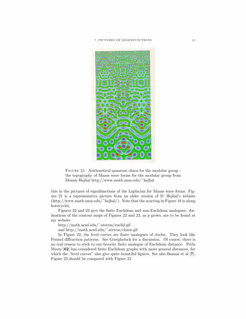
Figure 21. Arithmetical quantum chaos for the modular group -the topography of Maass wave forms for the modular group fromDennis Hejhal http://www.math.umn.edu/~hejhal

this in the pictures of eigenfunctions of the Laplacian for Maass wave forms. Fig-ure 21 is a representative picture from an older version of D. Hejhal’s website(http://www.math.umn.edu/~hejhal/). Note that the scarring in Figure 18 is alonghorocycles.

Figures 22 and 23 give the finite Euclidean and non-Euclidean analogues. An-imations of the contour maps of Figures 22 and 23, as p grows, are to be found atmy website

http://math.ucsd.edu/~aterras/euclid.gifand http://math.ucsd.edu/~aterras/chaos.gif.In Figure 22, the level curves are finite analogues of circles. They look like

Fresnel diffraction patterns. See Goetgheluck for a discussion. Of course, there isno real reason to stick to our favorite finite analogue of Euclidean distance. PerlaMyers [62] has considered finite Euclidean graphs with more general distances, forwhich the “level curves” also give quite beautiful figures. See also Bannai et al [7].Figure 23 should be compared with Figure 21.

42

Figure 22. Level "curves" for eigenfunctions of the adjacency ma-trix for finite Euclidean space with p = 163.

Figure 23. Level "curves" for eigenfunctions of the adjacency ma-trix for the finite upper half plane mod 163.

Bibliography

[1] G. Ahumada, Fonctions periodiques et formule des traces de Selberg sur les arbres, C. R.Acad. Sci. Paris, 305 (1987), 709-712.

[2] N. Allen, On the spectra of certain graphs arising from finite fields, Finite Fields Applics., 4(1998), 393-440.

[3] J. Angel, Finite upper half planes over finite fields, Finite Fields Applics., 2 (1996), 62-86.[4] J. Angel, B. Shook, A. Terras, C. Trimble, Graph spectra for finite upper half planes over

rings, Linear Algebra and its Applications, 226-228 (1995), 423-457.[5] C. Ballantine, Ramanujan type buildings, Canad. J. Math., 52 (2000), 1121-1148.[6] E. Bannai, Character tables of commutative association schemes, in Finite Geometries, Build-

ings, and Related Topics, (W. M. Kantor, et al, Eds.), Clarendon Press, Oxford, 1990, pp.105-128.

[7] E. Bannai, O. Shimabukuro, and H. Tanaka, Finite euclidean graphs and Ramanujan graphs,preprint.

[8] H. Bass, The Ihara-Selberg zeta function of a tree lattice, Internatl. J. Math., 3 (1992),717-797.

[9] C. Béguin, A. Valette, and A. Zuk, On the spectrum of a random walk on the discreteHeisenberg group and the norm of Harper’s operator, J. of Geometry and Physics, 21 (1997),337-356.

[10] N. Biggs, Algebraic Graph Theory, Cambridge U. Press, Cambridge, 1974.[11] O. Bohigas and M.-J. Giannoni, Chaotic motion and random matrix theories, Lecture Notes

in Physics, 209, Springer-Verlag, Berlin, 1984, pp. 1-99.[12] O. Bohigas, R.U. Haq, and A. Pandey, Fluctuation properties of nuclear energy levels and

widths: comparison of theory with experiment, in K.H. Böckhoff (Ed.), Nuclear Data forScience and Technology, Reidel, Dordrecht, 1983, pp. 809-813.

[13] B. Bollobas, Modern Graph Theory, Springer-Verlag, N.Y., 1998.[14] A. Borel and G. D. Mostow, Algebraic Groups and Discontinuous Subgroups, Proc. Symp.

Pure Math., IX, Amer. Math. Soc., Providence, 1966.[15] R. Brooks, The spectral geometry of k-regular graphs, J. d’Analyse, 57 (1991), 120-151.[16] P. Buser, Geometry and Spectra of Compact Riemann Surfaces, Birkhäuser, Boston, 1992.[17] P. Cartier, Harmonic analysis on trees, Proc. Symp. Pure Math., 26, Amer. Math. Soc.,

Providence, 1973, pp. 419-423.[18] C.-L. Chai and W.-C. W. Li, Character sums and automorphic forms, preprint.[19] M. D. Choi, G.A. Elliott, and N. Yui, Gauss polynomials and the rotation algebra, Inventiones

Math., 99 (1990), 225-246.[20] F. R. Chung, Spectral Graph Theory, Amer. Math. Soc., Providence, 1997.[21] F. Chung and S. Sternberg, Mathematics and the buckyball, American Scientist, 81 (1993),

56-71.[22] B. Cipra, What’s Happening in the Mathematical Sciences, 1998-1999, Amer. Math. Soc.,

Providence, RI, 1999.[23] D.M. Cvetkovic, M. Doob, and H. Sachs, Spectra of Graphs: Theory and Application, Acad-

emic, N.Y., 1979.[24] M. DeDeo, M. Martinez, A. Medrano, M. Minei, H. Stark, and A. Terras, Spectra of Heisen-

berg graphs over finite rings: histograms, zeta functions and butterflies, preprint (on the webat http://math.ucsd.edu/~aterras/heis.pdf).

[25] J. Elstrodt, Die Selbergsche Spurformel für kompakte Riemannsche Flächen, Jber. d. Dt.Math.-Verein., 83 (1981), 45-77.

43

44 BIBLIOGRAPHY

[26] J. Elstrodt, F. Grunewald, and J. Mennicke, Groups acting on Hyperbolic Space, Springer-Verlag, Berlin, 1998.

[27] R. Evans, Spherical functions for finite upper half planes with characteristic 2, Finite FieldsApplics, 3 (1995), 376-394.

[28] K. Feng and W. Li, Spectra of hypergraphs and applications, J. Number Theory, 60 (1996),1-22.

[29] A. Figá-Talamanca and C. Nebbia, Harmonic Analysis and Representation Theory forGroups acting on Homogeneous Trees, Cambridge U. Press, Cambridge, 1991.

[30] P. J. Forrester and A. Odlyzko, A nonlinear equation and its application to near-est neighbor spacings for zeros of the zeta function and eigenvalues of random ma-trices, in Proceedings of the Organic Math. Workshop, Invited Articles, located athttp://www.cecm.sfu.ca/~pborwein/

[31] J. Friedman (Ed.), Expanding Graphs, DIMACS Series in Disc. Math. and Th. Comp. Sci.,10, Amer. Math. Soc., Providence, 1993.

[32] P. Goetgheluck, Fresnel zones on the screen, Experimental Math., 2 (1993), 301-309.[33] F. Haake, Quantum Signatures of Chaos, Springer-Verlag, Berlin, 1992.[34] K. Hashimoto, Zeta functions of finite graphs and representations of p-adic groups, Adv.

Stud. Pure Math., 15, Academic, N.Y., 1989, pp. 211-280.[35] K. Hashimoto, Artin-type L-functions and the density theorem for prime cycles on finite

graphs, Internatl. J. Math., 3 (1992), 809-826.[36] D. A. Hejhal, The Selberg trace formula and the Riemann zeta function, Duke Math. J., 43

(1976), 441-482.[37] D.A. Hejhal, J. Friedman, M.C. Gutzwiller and A. M. Odlyzko (Eds.), Emerging Applications

of Number Theory, IMA Volumes in Math. and its Applications, 109, Springer-Verlag, N.Y.,1999.

[38] D. R. Hofstadter, Energy levels and wave functions of Bloch electrons in rational and irra-tional magnetic fields, Phys. Rev. B, 14 (1976), 2239-2249.

[39] N. Hurt, Finite volume graphs, Selberg conjectures, and mesoscopic systems: A review,preprint, 1998.

[40] Y. Ihara, On discrete subgroups of the two by two projective linear group over a p-adic field,J. Math. Soc. Japan,18 (1966), 219-235.

[41] S. Katok, Fuchsian Groups, Univ. of Chicago Press, Chicago, 1992.[42] N. Katz, Estimates for Soto-Andrade sums, J. Reine Angew. Math., 438 (1993), 143-161.[43] N. Katz, Gauss Sums, Kloosterman Sums, and Monodromy Groups, Princeton Univ. Press,

Princeton, N.J., 1988.[44] N. Katz and P. Sarnak, Random Matrices, Frobenius Eigenvalues and Monodromy, Amer.

Math. Soc., Providence, RI, 1999.[45] N. Katz and P. Sarnak, Zeroes of zeta functions and symmetry, Bull. Amer. Math. Soc., 36,

No. 1 (1999), 1-26.[46] M. Kotani and T. Sunada, Spectral geometry of crystal lattices, preprint.[47] A. Krieg, Hecke Algebras, Memoirs of Amer. Math. Soc., 435, Providence, 1990.[48] J.D. Lafferty and D. Rockmore, Fast Fourier analysis for SL2 over a finite field and related

numerical experiments, Experimental Math., 1 (1992), 115-139.[49] W. Li, Number Theory with Applications, World Scientific, Singapore, 1996.[50] W. Li, Ramanujan graphs and Ramanujan hypergraphs, Park City Lectures, 2002.[51] W. Li and P. Solé, Spectra of regular graphs and hypergraphs and orthogonal polynomials,

Europ. J. Combinatorics, 17 (1996), 461-477.[52] A. Lubotzky, Discrete Groups, Expanding Graphs, and Invariant Measures, Birkhäuser,

Boston, 1994.[53] A. Lubotzky, R. Phillips, and P. Sarnak, Ramanujan graphs, Combinatorica, 8 (1988), 261-

277.[54] A. Lubotzky, Cayley graphs, eigenvalues, expanders and random walks, Surveys in Combi-

natorics, 1995, Ed. P. Rowlinson, Cambridge U. Press, Cambridge, 1995, pp. 155-189.[55] F. J. Marquez, Ph. D. thesis, U.C.S.D., 2000.[56] M. G. Martínez, The finite upper half space and related hypergraphs, J. Number Theory, 84

(2000), 342-360.[57] M. G. Martínez, H. M. Stark, and A. Terras, Some Ramanujan hypergraphs associated to

GL(n,Fq), Proc. Amer. Math. Soc., 129 (2000), 1623-1629.

BIBLIOGRAPHY 45

[58] B. McKay, The expected eigenvalue distribution of a large regular graph, J. Lin. Alg. Appl.,40 (1981), 203-216.

[59] M. L. Mehta, Random Matrices and the Statistical Theory of Energy Levels, Academic, N.Y.,1990.

[60] M. Minei, Ph.D. Thesis, U.C.S.D., 2000.[61] M. Morgenstern, Ramanujan diagrams, S.I.A.M. J. Discrete Math., 7 (1994), 560-570.[62] P. Myers, Ph.D. Thesis, U.C.S.D., 1995.[63] H. Nagoshi, On arithmetic infinite graphs, Proc. Japan Acad., 76, Ser. A (2000), 22-25.[64] M. Rubinstein, Evidence for a spectral interpretation of zeros of L-functions, Ph.D. Thesis,

Princeton, 1998.[65] Z. Rudnick, Some problems in "quantum chaos" or statistics of spectra, Park City Lectures,

2002.[66] P. Sarnak, Some Applications of Modular Forms, Cambridge U. Press, Cambridge, 1990.[67] P. Sarnak, Arithmetic quantum chaos, Israel Math. Conf. Proc., 8 (1995), 183-236 (published

by the Amer. Math. Soc.).[68] C. Schmit, Quantum and classical properties of some billiards on the hyperbolic plane, in

Chaos and Quantum Physics, Eds. M.- J. Giannoni et al, Elsevier, N.Y., 1991, pp. 333-369.[69] A. Selberg, Harmonic analysis and discontinuous groups in weakly symmetric Riemannian

spaces with applications to Dirichlet series, J. Ind. Math. Soc., 20 (1954), 47-87.[70] J.-P. Serre, Trees, Springer-Verlag, N.Y., 1980.[71] J. Soto-Andrade, Geometrical Gel’fand models, tensor quotients, and Weil representations,

Proc. Symp. Pure Math., 47, Amer. Math. Soc., Providence, 1987, pp. 305-316.[72] D. Stanton, An introduction to group representations and orthogonal polynomials, Orthog-

onal Polynomials: Theory and Practice, Edited by P. Nevai and M. E. H. Ismail, Kluwer,Dordrecht, 1990, 419-433.

[73] H.M. Stark and A. Terras, Zeta functions of finite graphs and coverings, Advances in Math.,121 (1996), 124-165.

[74] H.M. Stark and A. Terras, Zeta functions of finite graphs and coverings, Part II, Advancesin Math., 154 (2000), 132-195.

[75] H. M. Stark and A. Terras, Artin L-functions of graph coverings, Proceedings of the Con-ference on Dynamical, Spectral and Arithmetic Zeta Functions, Contemporary Math., 290(2001), 181-195.

[76] H. M. Stark and A. Terras, Zeta functions of graph coverings, Proc. DIMACS Workshop onUnusual Applications of Number Theory, ed. Melvyn B. Nathanson, in press.

[77] M. E. Starzak, Mathematical Methods in Chemistry and Physics, Plenum, N.Y., 1989.[78] S. Sternberg, Group Theory and Physics, Cambridge U. Press, Cambridge, 1994.[79] A. Strömbergsson, On the zeros of L-functions associated to Maass waveforms, International

Math. Res. Notices, 15 (1999), 839-851.[80] T. Sunada, Fundamental groups and Laplacians, Lecture Notes in Math., 1339, Springer-

Verlag, N.Y., 1987, p. 248-277.[81] A. Terras, Survey of spectra of Laplacians on finite symmetric spaces, Experimental Math.,

5 (1996), 15-32.[82] A. Terras, Fourier Analysis on Finite Groups and Applications, Cambridge Univ. Press,

Cambridge, U.K., 1999.[83] A. Terras, Harmonic Analysis on Symmetric Spaces and Applications, I,II, Springer-Verlag,

N.Y., 1985, 1988.[84] A. Terras, Statistics of graph spectra for some finite matrix groups: Finite Quantum Chaos,

Proc. International Workshop on Special Functions, June, 1999, C. Dunkl et al, Eds., WorldScientific, Singapore, 2000, pp. 351-374.

[85] A. Terras, Comparison of Selberg’s trace formula with its discrete analogues, Proc. DIMACSWorkshop on Unusual Applications of Number Theory, ed. Melvyn B. Nathanson, in press.

[86] A. Terras, Finite Quantum Chaos, American Math. Monthly, 109 (2002), 121-139.[87] A. Terras and D. Wallace, Selberg’s Trace Formula on the k-Regular Tree and Applications,

International J. of Math. and Math. Sciences, 2003, No. 8 (Feb., 2003), 501-526.[88] P. D. Tiu and D. Wallace, Norm quadratic residue codes, IEEE Trans. Inform. Theory, 40

(3), (1994), 946-949.[89] A. B. Venkov and A. M. Nikitin, The Selberg trace formula, Ramanujan graphs and some

problems of mathematical physics, Petersburg Math. J., 5 (3), (1994), 419-484.

46 BIBLIOGRAPHY

[90] A. Weil, Collected Papers, Vols. I-III, Springer-Verlag, Berlin, 1979.[91] E. P. Wigner, Random matrices in physics, S.I.A.M. Review, 9, No. 1 (1967), 1-23.