Audits or Distortions: The Optimal Scheme to Enforce

Self-Employment Income Taxes∗

Eduardo Zilberman

Department of Economics

New York University

July 2010

Abstract

I investigate the optimal auditing mechanism for a net revenue maximizer tax collec-

tion agency that in addition to reported profits, it also observes the level of employment

at each firm. Each firm is managed and owned by a single entrepreneur. Firms’ pro-

ductivity is heterogeneous as managerial ability is random. Since auditing probabilities

depend on employment, labor decisions are distorted. The optimal auditing scheme

and corresponding labor schedule are discontinuous and non-monotone in ability. In

intermediate audit costs, the less productive entrepreneurs face auditing probabilities

that increase with their managerial ability, whereas the ablest ones are not audited. A

quantitative exploration suggests that if the optimal auditing scheme was adopted in

practice, net revenue would increase by at least 59%.

Keywords: optimal auditing, tax evasion, entrepreneurship, mechanism design.

JEL Classification: D21, H26.

∗E-mail: eduardo.zilberman@nyu.edu. I thank Ennio Stachetti for insightful guidance. I also thank TiagoBerriel, Ryan Booth, Bernardo da Silveira, Raquel Fernandez, Vivian Figer, Sean Flynn, Renato Gomes,Pedro Hemsley, Boyan Jovanovic, Alessandro Lizzeri, Thomas Mertens, Nicola Persico, Nikita Roketskiy,Tomasz Sadzik, Daniel Xu, Joyce Wong, and participants at seminars for helpful comments and discussions.I am especially indebted to Saki Bigio, whose comments and discussions were invaluable. All errors are mine.

1

1 Introduction

The optimal income tax enforcement literature1 has mostly focused on individual taxpayers

whose income is either exogenous or solely remunerates labor supply.2 However, Slemrod

[2007] reports that in the U.S., due to third-party reporting, only 1 percent of wages and

salaries are underreported to the tax collection agency (henceforth the IRS). In contrast,

43 percent of individual business income, which is mostly self-reported, is underreported.3

Hence, given that wages taxes are practically enforced, the number of workers at each firm

seems to be easily observable by the IRS. This paper asks the following: given that, in

addition to reported income, employment at each firm is also observable, how should a net

revenue maximizer IRS monitor heterogeneous entrepreneurs?4 In particular, the source of

heterogeneity is a random managerial ability.

By conditioning its monitoring strategy on employment, the IRS also indirectly distorts

labor input to enforce taxes. As a result, employment is distorted in almost every firm.

Moreover, if the cost to audit is not too high, the less productive entrepreneurs face auditing

probabilities that increase with their managerial ability, whereas the ablest ones are not

audited. At some threshold level of ability, the monitoring strategy discontinuously drops.

Hence, the optimal auditing scheme and labor schedule are not monotone in ability.

In Section 2, I introduce a variant of Bigio and Zilberman [forthcoming]’s two stage game

to study optimal self-employment income tax enforcement. A self-employed is a risk-neutral

entrepreneur who owns and manages a single firm. In particular, an entrepreneur experiences

a random managerial ability, also her privately observed type, that enhances productivity in

a plant exhibiting decreasing returns to scale. Production is carried out by a team of workers.

Entrepreneurs can underreport income, that is the profits generated by their own firms, in

order to evade taxes. If a firm is audited, true income is uncovered, and the entrepreneur

1 The seminal paper is Reinganum and Wilde [1985], which is inspired by the costly state verificationmodel of Townsend [1979]. Notable contributions are Border and Sobel [1987], Mookherjee and Png [1989],Cremer et al. [1990], Sanchez and Sobel [1993], Cremer and Gahvari [1996], Macho-Stadler and Perez-Castrillo [1997], Chander and Wilde [1998], and Bassetto and Phelan [2008]. The first theoretical workon tax noncompliance is Allingham and Sandmo [1972], which builds on the work of Becker [1968] on theeconomics of crime. Recent surveys are Andreoni et al. [1998], Slemrod and Yitzhaki [2002], and Sandmo[2005].

2A recent exception is Parker [2010], who introduces entrepreneurship and dynamic incentives in a two-period model. Armenter and Mertens [2010] and Ravikumar and Zhang [2010] also study the role of auditsin a dynamic environment.

3These figures account for 10 and 109 billion dollars, respectively. Kleven et al. [2010], for instance,define the tax evasion rate as the share of reported income that is underreported. Using data from Denmark,they estimate it as being 8.1% for self-employment income, 0.4% for earnings, 0.3% for third-party reportedincome, and 37% for self-reported income.

4In this paper, firms and entrepreneurs make up a single unit. Henceforth, I use both terms interchange-ably.

2

who owns this firm must pay a penalty.

In the first stage, given the managerial ability distribution, the IRS commits to a costly

monitoring strategy dependent on both reported income and labor input, assumed to be

costlessly observable. In the second stage, firms take into account this monitoring strategy

and choose labor input and reported income. Hence, labor is not only a factor input, but

also a signal of the true income. At a production cost, labor can be strategically distorted

to signal a lower income to the IRS.

To solve this model, I follow a mechanism design approach, in which the choice of labor

and reported income are delegated to the IRS. Due to the revelation principle, it is enough

to focus within the class of direct mechanisms that respect incentive compatibility and

individual rationality. That is, an agent reports her type (i.e., her managerial ability) and is

then assigned a labor input to employ, an amount to report as profits, and a probability she

is audited with. The mechanism is designed such that agents report truthfully their types,

and derive at least their reservation values.

Since an entrepreneur can always declare her true profits and pay the right amount of

taxes, her reservation value is the post-tax truthfully declared profits, which is increasing

in the managerial ability. This type-dependent reservation value generates countervailing

incentives. That is, on the one hand, an entrepreneur is willing to understate her type in

order to pay less taxes. On the other hand, she is willing to overstate her type in order

to be assigned a higher reservation value. In this specific environment, the incentives to

understate (overstate) are stronger for high-ability (low-ability) types. Therefore, as audits

are also designed to deter type misreport, countervailing incentives are one of the driving

forces that make the optimal auditing scheme not monotone in ability.

The other driving force is the joint condition of the monitoring strategy on both reported

income and labor input. If it depends only on reported income, a non-increasing monitoring

strategy is necessary to verify incentive compatibility. If it is also conditioned on labor input,

this requirement is relaxed. In Sections 3 and 4.1, I discuss this result in details.

If employment at each firm is unobservable, the model presented in this paper collapses

to a variant of the one in Sanchez and Sobel [1993]. In this context, the optimal monitoring

strategy is a cut-off rule. Every entrepreneur below a certain threshold type is audited with

constant intensity, whereas those above it are not monitored at all. In equilibrium, only

low-ability entrepreneurs report income honestly, while high-ability entrepreneurs report the

income of the threshold type. Consequently, the richest entrepreneurs evade proportionally

more, introducing a regressive bias in the effective tax rate.

If labor input is observable, on top of audits, the IRS can also use labor distortions

to provide incentives and enforce taxes. The solution to this problem has the following

3

properties: (1) as in a standard mechanism design problem, the top-type is not distorted;

(2) in the top range of the type distribution, audits are never used, and labor is distorted

downwards to prevent high-ability entrepreneurs from understating their types; (3) below

some threshold type, stronger incentives for entrepreneurs to overstate their types, and be

assigned a higher reservation value, limit the further use of distortions to provide incentives.

Individual rationality binds in this region; (4) if the audit cost is too high, only labor

distortions are used to provide incentives; (5) if the audit cost is not too high, audits and

labor distortions are optimally combined to enforce taxes. In the bottom range of the

type distribution, both the optimal monitoring strategy and labor schedule are increasing

in ability. At the threshold type, they drop discontinuously; (6) every entrepreneur reports

dishonestly; Finally, (7) the effective tax rate is higher in the middle of the type distribution,

thus the overall regressive (or progressive) bias that arises from evasion is unknown.

The role of costly audits as a tool to maximize government revenue is twofold: First,

it enforces taxes from those that are audited; Second, it provides incentives by preventing

misreport from other types, which allows the IRS to require higher income declarations from

them. Similarly, labor distortions can be used to provide incentives, but only at a production

cost that diminishes revenue collection. The optimal mechanism balances the use of these

two tools in a way that preserves incentive compatibility and individual rationality, and also

maximizes net revenue collection.

In Section 4, I present an example that summarizes the intuition behind these results,

which are analytically derived in Section 5. In Section 6, I discuss some generalizations to

the model.

On the technical side, this paper solves a mechanism design problem with two choice vari-

ables that goes beyond quasi-linearity, and features type-dependent individual constraints.

Moreover, the solution method accounts for the presence of discontinuities.

In Section 7, I explore quantitatively the implications of this mechanism. In particular, I

establish a lower bound to the net revenue increase if the mechanism developed in this paper

was counterfactually adopted. Under the assumption that the U.S. is a “relatively free-

distortion” competitive economy,5 I use data on employment and entrepreneurship from the

Survey of Consumer Finance to impose some discipline on the managerial ability distribution.

Results suggest that once adopted, the optimal mechanism can substantially increase

revenue and reduce evasion in comparison with the U.S. data. In particular, among nonfarm

sole-proprietors, for a conservative choice of parameters, revenue collection increases by at

least 59%, and the fraction of reported income is at least 86%, as opposed to 43% documented

5By relatively free-distortion, I mean an economy in which policies do not target the firm size. Bycompetitive, I mean an economy in which entrepreneurs take prices as given and maximize expected profits.

4

in Slemrod [2007]. Section 8 concludes.

2 Model

I consider a two-stage game in which entrepreneurs remit taxes to the IRS. Taxes may be

potentially evaded. In the first stage, the IRS commits to a monitoring strategy that depends

both on observable labor input and reported income. In the second stage, firms take into

account the monitoring strategy, and choose labor input and reported income.

There is a continuum of firms of measure one. Each firm is owned and managed by a

single entrepreneur, who experiences a random managerial ability z, which is her privately

observed type. I assume z is independently and identically distributed according to G, with

density g = G′ uniformly bounded away from zero, and compact support [z, z] with z ≥ 0.

I also assume g is continuously differentiable.

There is a single good produced with a single observable input, labor n.6 The production

technology is znα, with α ∈ (0, 1) common to all firms. Let wages be the numeraire, and p

be the price of the good, thus pre-tax profits are π(n, z) = pznα−n. Notice that the efficient

level of employment is n∗(z) = (αpz)1

1−α .

Decreasing returns to scale are important to generate positive profits in a competitive

environment, otherwise the posed question would be trivial. This specific functional form

is chosen for tractability. I discuss the consequences of adopting a more general production

function in Section 6.1. In particular, I show that the production technology can be gener-

alized to znα0∏I

i=1 kαii , with α0 +

∑Ii=1 αi ∈ (0, 1) and αi ≥ 0 for i = 0, .., I, as long as only

n is observable. This generalization is important because it extends the scope in which the

model can be applied. For example, even if unskilled labor can be hidden, the IRS might

still observe skilled labor or any other input.

A profit tax rate, τ , is imposed exogenously by the government. After observing her own

type z, the entrepreneur decides how much labor to hire and income to report to the IRS. I

denote reported profits by x ≥ 0, so τx is the amount paid out as taxes, and τ(π(n, z)− x)

is the amount evaded by the entrepreneur. The IRS (the principal) costlessly observes labor

n and reported income x. However, it is able to observe ability z, and hence actual income,

only if it audits the firm at a constant cost c > 0. If an entrepreneur is audited, she is

assessed by maxµτ(π(n, z)−x), 0, where µ > 1 is a linear penalty on the amount evaded.7

6In some contexts, labor might not be readily observable. However, n can be any other observable inputfactor, such as the physical capital of a plant, for example.

7Implicitly, I assume all penalties are enforced even if µτ(π(n, z) − x) > π(n, z) − τx, that is, penaltiesare higher than post-tax profits. If limited liability is a concern, I could assume that µ ∈ (1, 1

τ ], which isenough to guarantee penalties are payable only with post-tax profits.

5

Penalties are assumed to be linear for tractability, otherwise I would not be able to rewrite

the IRS problem in terms of expected informational rents, a trick that simplifies the solution.

Note that the IRS does not reward overreporting. Hence, without loss of generality,

I restrict the set of reported income to be [0, π(n, z)], and set maxµτ(π(n, z) − x), 0 =

µτ(π(n, z)− x).

In this paper, the IRS is an agency responsible only for auditing and collecting taxes.

Choosing tax rates and penalties is beyond its scope.8 In particular, taxes would be fully

enforced without cost if penalties were arbitrarily large, that is µ → ∞. However, many

authors argue that an abusive use of penalties is limited by other reasons, such as a common

ethical norm,9 or more economically, to restrain the power of corruptible self-interested

enforcers.10

The IRS knows the distribution of firms, G. In the first stage, in order to maximize

expected net revenue, given G, the IRS commits to a monitoring strategy, which is an audit

probability function, ϕ(n, x), that depends both on employment and reported income.

As Andreoni et al. [1998] argue, assuming that the IRS objective is to maximize expected

net revenue, instead of a welfare criteria, seems a reasonable positive description of how many

tax agencies behave in practice. However, most tax agencies do not explicitly commit to a

monitoring strategy that depends on available information. Hence, I justify this assumption

on a normative ground. If net revenue collection is the main concern, as in periods of high

budget deficits, the best the IRS can do is to commit to a monitoring strategy that depends

on all costlessly observable variables.11

In the second stage, given ϕ, the entrepreneur’s problem is to maximize her expected

profits:

maxn≥0,x∈[0,π(n,z)]

π(n, z)− τx− ϕ(n, x)µτ(π(n, z)− x).

Notice that labor is not only a factor input, but also a signal of the true income. Hence, at

a production cost, labor input can be strategically distorted to signal a lower income to the

IRS.

Before proceeding with the analysis, I solve for the full-information case, that is, when

z is observable. Let the monitoring strategy, also a function of z in this case, be denoted

8These variables are usually chosen by other government spheres like the Treasury or Congress. Forexample, in August 2007, the U.S. Government Accountability Office (U.S. GAO) published a report(http://www.gao.gov/new.items/d071062.pdf) suggesting the Congress to require IRS to periodically ad-just penalties for inflation.

9Rosen [2005], for example, argues that “existing penalty systems try to incorporate just retribution.Contrary to the assumptions of the utilitarian framework, society cares not only about the end result (gettingrid of the cheaters) but also the processes by which the result is achieved.”

10See Polinsky and Shavell [2000] for a survey.11See Erard and Feinstein [1994] for a model in which the IRS does not commit to a monitoring strategy.

6

by ϕ∗(n, x, z). In the second stage, a firm z weakly prefers to declare its true profits π(n, z)

rather than underreport x < π(n, z) whenever ϕ∗(n, x, z) ≥ 1µ. Indeed, by comparing ex-

pected profits,

(1− τ)π(n, z) ≥ π(n, z)− τx− ϕ∗(n, x, z)µτ(π(n, z)− x) ⇐⇒ ϕ∗(n, x, z) ≥ 1

µ.

Similarly, the IRS weakly prefers that an entrepreneur z declares her true profits π(n, z)

rather than underreports x < π(n, z) whenever it chooses ϕ∗(n, x, z) ≤ 1µ

in the first stage.

Indeed, by comparing expected revenue,

τπ(n, z) ≥ τx+ ϕ∗(n, x, z)µτ(π(n, z)− x) ⇐⇒ ϕ∗(n, x, z) ≤ 1

µ.

Hence, the best the IRS can do is to induce every entrepreneur z to produce efficiently

and report her true profits π(n∗(z), z), without spending resources. This is achieved by the

following monitoring strategy:

ϕ∗(n, x, z) =

1µ

if x 6= π(n∗(z), z) or n 6= n∗(z)

0 otherwise.

I use the superscript ∗ to denote the full-information solution in order to highlight that it in-

duces the efficient employment per firm. This mechanism works only through off-equilibrium

threats. As long as the IRS commits to this monitoring technology, it enforces all taxes at

no cost.

If the IRS does not observe z, an adverse selection problem arises. In order to increase

her expected profits, an entrepreneur may distort her labor decision and report less income.

To solve this problem, I follow a mechanism design approach. By the revelation principle,

it is enough to restrict attention to the class of direct mechanisms that respect incentive

compatibility and individual rationality. That is, an agent reports her type, say z, and is

then assigned n(z), x(z), and φ(z), where φ is the direct monitoring strategy, defined on

[z, z]. In particular, the mechanism is designed such that an entrepreneur reports truthfully

her type, that is z = z, and derives at least her reservation value. I assume that n, x, and φ

are piecewise continuously differentiable functions of z.

The idea is to solve for the optimal direct mechanism n(z), x(z), φ(z)z, and then con-

struct a mapping between φ and ϕ in the following way:

ϕ(n, x) =

φ(z) if there exists z s.t. (n, x) = (n(z), x(z))

ϕ(n, x) otherwise,

7

where ϕ(n, x) is a high enough off-equilibrium threat to deter any deviation to such (n, x).12

Let a type z entrepreneur’s expected profits be

Π(n, x, φ, z) = π(n, z)− τx− φµτ(π(n, z)− x).

Given G, the IRS problem is to

maxn(z),x(z),φ(z)z

∫ z

z

τx(z) + φ(z)[µτ(π(n(z), z)− x(z))− c] dG(z)

s.t.

(F) φ(z) ∈ [0, 1] , x(z) ∈ [0, π(n(z), z)], n(z) ≥ 0,∀z ∈ [z, z]

(IR) Π(n(z), x(z), φ(z), z) ≥ (1− τ)π(n∗(z), z),∀z ∈ [z, z]

(IC) Π(n(z), x(z), φ(z), z) ≥ Π(n(z), x(z), φ(z), z),∀z, z ∈ [z, z]× [z, z].

Feasibility (F) requires that the set of offered menus corresponds to feasible probabilities,

income declarations, and labor input.

Incentive compatibility (IC) requires that entrepreneurs do not have incentives to choose

a different allocation from the one designed by the mechanism for them.

The set of individual rationality (IR) constraints merits some digression. As opposed to

other mechanism design applications, such as monopoly screening, the “supply” of agent’s

choice variables (n and x, in this paper) is not controlled by the principal. Thus an agent

can also deviate to an off-scheduled pair (n, x). In particular, a type z entrepreneur can

always declare her true profits, x = π(n, z), and pay the right amount of taxes. If this is the

case, her post-tax profits are (1 − τ)π(n, z), and thus any mechanism must assign at least

(1− τ)π(n∗(z), z) to the entrepreneur.13

In principle, entrepreneurs could also deviate to other off-scheduled allocations. However,

given that any mechanism must assign at least (1− τ)π(n∗(z), z) to each entrepreneur, this

problem is circumvented by setting ϕ(n, x) = 1/µ for all off-scheduled (n, x). Indeed, if

ϕ(n, x) = 1/µ, entrepreneurs prefer to declare their true profits instead of x.14 Consequently,

(IR) deters off-scheduled deviations, and thus it also plays a role to guarantee that incentives

are compatible.

Figure 1 illustrates the role (IR) is playing in the model. Suppose the curve depicted

in the left (n, x)-plan represents the optimal mechanism. That is, each point in this curve

12Incentive compatibility guarantees that for all z1 6= z2 such that (n(z1), x(z1)) = (n(z2), x(z2)), thenφ(z1) = φ(z2).

13Recall that n∗(z) is the efficient labor, and it maximizes (1− τ)π(n, z).14Recall that (1− τ)π(n, z) ≥ π(n, z)− τx− ϕ(n, x)µτ(π(n, z)− x) if and only if ϕ(n, x) ≥ 1/µ.

8

is associated with a single type, and thus with an audit probability φ(z). If any pair (n, x)

outside this curve is audited with intensity 1/µ, (IR) ensures that entrepreneurs stick to the

curve. In other words, through off-equilibrium threats, the IRS can indirectly implement the

optimal allocation.

Figure 1: Implementation.

However, in practice, it is not a sensible recommendation for policy to audit intensively

whoever reports much more than expected. The right plot of Figure 1 shows an alternative

way to implement the optimal mechanism. Those that report a lower income than expected

are audited with a high intensity. Those that report above some threshold curve, the dashed

line, are not audited. In the shadow region, between the dashed- and the full-line, auditing

intensities are set in a way to deter off-schedule deviations, but not necessarily equal to 1/µ.

Using Lewis and Sappington [1989] terminology, this model displays countervailing in-

centives. On the one hand, a firm has incentives to underreport z and pay less taxes. On the

other hand, since the reservation value, (1−τ)π(n∗(z), z), is increasing in z, an entrepreneur

is also tempted to overstate z and be assigned a higher value. Therefore, the solution is not

necessarily characterized by the full informational rent extraction of the lowest type, and

standard tricks in the literature are not readily applicable here.

Sanchez and Sobel [1993] and Bigio and Zilberman [forthcoming] also consider a similar

environment to study optimal enforcement policies. The former paper assumes that income

is exogenous, thus auditing probabilities can not be conditioned on employment. The latter

conditions the monitoring strategy only on labor input. In these papers, the IRS is assigned

a fixed budget, which is exhausted in order to maximize revenue.15 Moreover, Sanchez and

15Operationally, both environments are similar since a budget constraint of the form∫φ(z)cdG(z) ≤ C,

where C is the assigned budget, can be cast in the principal’s problem using a Lagrange multiplier, sayξ ≥ 0. Hence, a revenue maximizer IRS optimizes

∫τx(z) + φ(z)[µτ(π(n(z), z)− x(z))− ξc] dG(z) + ξC

subject to (F), (IR), and (IC).

9

Sobel [1993] consider a more general tax schedule, while Bigio and Zilberman [forthcoming]

consider more general production and audit cost functions. For simplicity, I specify functional

forms for these primitives, although in Section 6, I discuss to what extent they can be relaxed.

Finally, I refer these papers for further discussions on most of the assumptions used here.

3 Implementability

Let U denote the informational rent an agent gets. Hence,

U(z) = maxz∈[z,z]

π(n(z), z)− τx(z)− φ(z)µτ(π(n(z), z)− x(z))− (1− τ)π(n∗(z), z) . (1)

The following lemma is standard and states necessary and sufficient conditions for the

incentive compatibility constraint be globally satisfied.

Lemma 1. Incentive compatibility is verified if and only if

(LIC) :dU

dz(z) = (1− φ(z)µτ)pn(z)α − (1− τ)pn∗(z)α, a.e.

(M) : n(z)α(1− φ(z)µτ) is non-decreasing,

and that U is absolutely continuous.

These two conditions are crucial to understand the results in this paper. The local incen-

tive compatibility (LIC) follows from applying the envelope theorem to (1), and evaluating

the resulting equation at z = z. It specifies the required slope of the informational rent,

U(z), to induce truthtelling. Notice that (LIC) provides a clear interpretation of counter-

vailing incentives. Indeed, the first term captures the incentives to understate z, and declare

less profits, whereas the second term captures the temptation to overstate z, and thus be

assigned a higher reservation value.

(M) is a variant of the monotonicity condition present in the mechanism design literature.

If, for example, on-equilibrium audits are ruled out from the problem, that is φ(z) = 0 for

all z, then (M) collapses to n(z) being non-decreasing. Intuitively, by setting high enough

off-equilibrium auditing intensities, the IRS can always shape reported income x to work as if

it were compensatory transfers, as in a textbook mechanism design problem (e.g., Fudenberg

and Tirole [1991]). Hence, a non-decreasing labor schedule is sufficient for implementability.

On the other hand, if the monitoring strategy did not depend on n, then labor distortions

could not be used to provide incentives. Hence, (M) would be equivalent to φ(z) being non-

10

increasing. This is a standard property in the optimal tax enforcement literature.16 It

prevents higher-types from mimicking a low-type in order to pay less taxes. Following the

steps in Bigio and Zilberman [forthcoming], one can show that if labor is unobservable, then

the next proposition, originally from Sanchez and Sobel [1993], holds.

Let the superscript x denote the optimal solution when the monitoring strategy is con-

ditioned only on reported income.

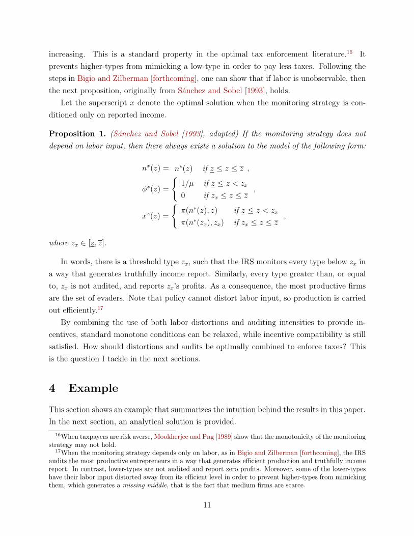
Proposition 1. (Sanchez and Sobel [1993], adapted) If the monitoring strategy does not

depend on labor input, then there always exists a solution to the model of the following form:

nx(z) = n∗(z) if z ≤ z ≤ z ,

φx(z) =

1/µ if z ≤ z < zx

0 if zx ≤ z ≤ z,

xx(z) =

π(n∗(z), z) if z ≤ z < zx

π(n∗(zx), zx) if zx ≤ z ≤ z,

where zx ∈ [z, z].

In words, there is a threshold type zx, such that the IRS monitors every type below zx in

a way that generates truthfully income report. Similarly, every type greater than, or equal

to, zx is not audited, and reports zx’s profits. As a consequence, the most productive firms

are the set of evaders. Note that policy cannot distort labor input, so production is carried

out efficiently.17

By combining the use of both labor distortions and auditing intensities to provide in-

centives, standard monotone conditions can be relaxed, while incentive compatibility is still

satisfied. How should distortions and audits be optimally combined to enforce taxes? This

is the question I tackle in the next sections.

4 Example

This section shows an example that summarizes the intuition behind the results in this paper.

In the next section, an analytical solution is provided.

16When taxpayers are risk averse, Mookherjee and Png [1989] show that the monotonicity of the monitoringstrategy may not hold.

17When the monitoring strategy depends only on labor, as in Bigio and Zilberman [forthcoming], the IRSaudits the most productive entrepreneurs in a way that generates efficient production and truthfully incomereport. In contrast, lower-types are not audited and report zero profits. Moreover, some of the lower-typeshave their labor input distorted away from its efficient level in order to prevent higher-types from mimickingthem, which generates a missing middle, that is the fact that medium firms are scarce.

11

In this example, I assume z follows a uniform distribution with support [2, 3], α = 1/2,

p = 1, µτ = 1, and τ = 0.25.18

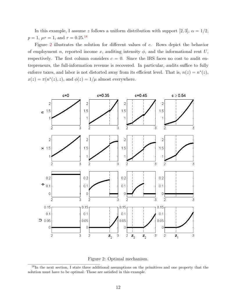
Figure 2 illustrates the solution for different values of c. Rows depict the behavior

of employment n, reported income x, auditing intensity φ, and the informational rent U ,

respectively. The first column considers c = 0. Since the IRS faces no cost to audit en-

trepreneurs, the full-information revenue is recovered. In particular, audits suffice to fully

enforce taxes, and labor is not distorted away from its efficient level. That is, n(z) = n∗(z),

x(z) = π(n∗(z), z), and φ(z) = 1/µ almost everywhere.

Figure 2: Optimal mechanism.

18In the next section, I state three additional assumptions on the primitives and one property that thesolution must have to be optimal. Those are satisfied in this example.

12

On the other hand, if c is high enough as in the forth column,19 it is too costly to

use auditing probabilities in equilibrium. Therefore, only labor distortions are used. As

in a standard mechanism design problem, the top-type is not distorted away from the full-

information case, that is n(z) = n∗(z) and φ(z) = 0, while labor is distorted downwards

to provide incentives. Below a threshold type, call it z1, depicted by the dashed-line, the

individual rationality binds, which places a limit on the further use of distortions to provide

incentives. In particular, employment has to be adjusted to keep U(z) = 0 for z ≤ z1. As

opposed to problems without countervailing incentives, the individual rationality can bind

at intermediate types.

The most interesting case is when c assumes intermediate values, as in the second and

third columns, for c = 0.35 and c = 0.45, respectively.

Similarly, the “non-distortion at the top” result also holds here, and labor is distorted

downwards up to a threshold type, call it z2, which is the (right) dashed-line in the second

(third) column. In this region, only distortions are used.

Below z2, up to another threshold, call it z3, which is the left dashed-line in the second

column,20 the IRS combines both distortions and audits to enforce taxes. In particular, for

z ∈ [z3, z2), both φ(z) and n(z) are increasing. Moreover, at z = z2, both the labor input

and the auditing intensity drop discontinuously (this discontinuity might not be visible in

Figure 2, so I reproduce the plots for c = 0.35 in Figure 3). In this region, the individual

rationality binds.

To understand the intuition behind the jump, notice that, in order to increase net revenue,

the use of audits are twofold: (1) it enforces taxes from those that are audited; (2) it

prevents deviations from other types, allowing the IRS to require higher income declarations

from them. In the top range of the type distribution, entrepreneurs have strong incentives

to understate their type, and then pay less taxes. Hence, monitoring those at the top is

effective to enforce their taxes, but ineffective to prevent deviations from other types. The

jump of the monitoring strategy at z2 balances these two goals. It allows the IRS to audit

and enforce taxes from a somewhat set of productive types, at the same time that establishes

a lower bound on the income reported by the highest types.

If the monitoring strategy depended only on reported income, as in Proposition 1, the

same reasoning would justify a discontinuously drop of the monitoring strategy. However,

the ablest entrepreneurs do not report, or bunch at, the threshold type income anymore.

Intuitively, by continuously distorting labor downwards to provide incentives, the IRS can

separate the equilibrium and design an increasing reported income schedule. The jump in

19In this particular example, for c ≥ 0.54.20In this example, for all c > 0.375, z3 > z. If c ≤ 0.375, z3 = z.

13

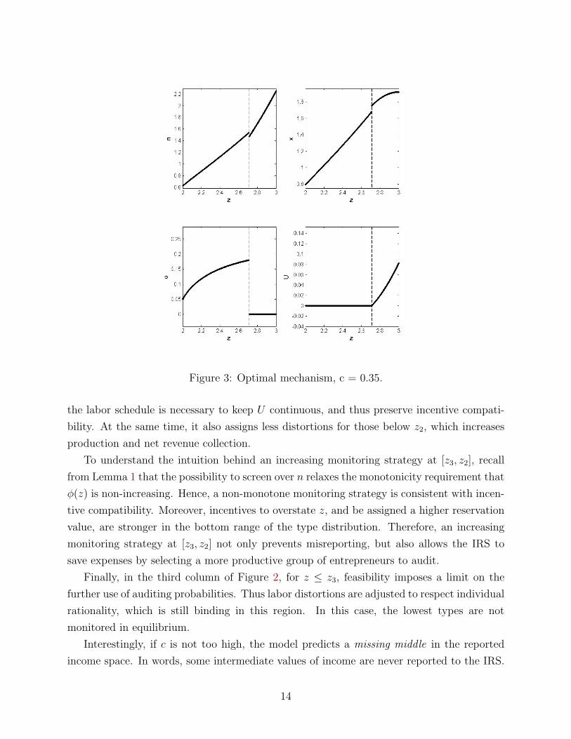
Figure 3: Optimal mechanism, c = 0.35.

the labor schedule is necessary to keep U continuous, and thus preserve incentive compati-

bility. At the same time, it also assigns less distortions for those below z2, which increases

production and net revenue collection.

To understand the intuition behind an increasing monitoring strategy at [z3, z2], recall

from Lemma 1 that the possibility to screen over n relaxes the monotonicity requirement that

φ(z) is non-increasing. Hence, a non-monotone monitoring strategy is consistent with incen-

tive compatibility. Moreover, incentives to overstate z, and be assigned a higher reservation

value, are stronger in the bottom range of the type distribution. Therefore, an increasing

monitoring strategy at [z3, z2] not only prevents misreporting, but also allows the IRS to

save expenses by selecting a more productive group of entrepreneurs to audit.

Finally, in the third column of Figure 2, for z ≤ z3, feasibility imposes a limit on the

further use of auditing probabilities. Thus labor distortions are adjusted to respect individual

rationality, which is still binding in this region. In this case, the lowest types are not

monitored in equilibrium.

Interestingly, if c is not too high, the model predicts a missing middle in the reported

income space. In words, some intermediate values of income are never reported to the IRS.

14

Moreover, two different types might be assigned the same labor input.

In the next three subsections, I use this example to discuss further insights from the

model. Namely, I discuss the case in which τ = 1, the implications of the optimal mechanism,

and the potential net revenue gain and efficiency loss from adopting this mechanism.

4.1 τ = 1

τ = 1 describes a context in which the principal aims to fully appropriate the agent’s profits.

This action can be legitimate, as the example of a holding company requiring reports on

the profitability of its subsidiaries. But it can also be illegitimate, as the example of a local

mafia extorting business owners.

If τ = 1, the monitoring strategy becomes the standard cut-off rule. That is, every z

below a threshold type is audited with intensity 1/µ, while every z above it is not monitored.

Intuitively, the reservation value, (1 − τ)π(n∗(z), z), ceases to be type-dependent, and thus

countervailing incentives are ruled out. (LIC) and (M) become

(LICτ=1) :dU

dz(z) = (1− φ(z)µ)pn(z)α, a.e.

(Mτ=1) : n(z)α(1− φ(z)µ) is non-decreasing,

respectively. Interestingly, a non-monotone monitoring strategy could be implementable,

although it is not optimal.

Therefore, a type-dependent reservation value is necessary to break the monotonicity

result that φ(z) is non-increasing. But is it sufficient? No, if labor input is not observable,

Proposition 1 follows and the optimal monitoring strategy is the cut-off rule. Assume τ < 1,

so (LIC) and (M) become

(LICx) :dU

dz(z) = (1− φ(z)µτ)pn∗(z)α − (1− τ)pn∗(z)α, a.e.

(Mx) : φ(z) is non-increasing,

respectively. The IRS can not implement a non-monotone monitoring strategy.

Consequently, countervailing incentives and the possibility to screen over labor are the

driving forces behind the results in this paper.

4.2 Implications

In a risk-neutral environment, in which the IRS can credibly commit to a monitoring strategy

that depends only on reported income, the cut-off audit rule derived in Proposition 1 is a

15

remarkable robust result. However, its policy implications are unsatisfactory for two reasons.

First, the amount underreported as a fraction of income increases with income, introducing

a regressive bias on effective taxes. Second, only those that declare income honestly will

be audited, which are precisely the poorest taxpayers. In this section, I show how these

implications change once the monitoring strategy also depends on labor.

4.2.1 Underreported income

Let underreported income as a fraction of true income be 1 − x(z)/π(n(z), z). Figure 4

plots this variable for different values of c. The full-line represents the optimal mechanism

when the monitoring strategy depends on both reported profits and labor input, while the

dashed-line conditions the monitoring strategy only on the former.21

Figure 4: Underreported income as a fraction of true income.

In contrast with the previous literature, every taxpayer evades in the model. More

interestingly, the relationship between the fraction of income that is underreported and

income is non-monotone and discontinuous. In particular, those in the bottom and top

underreport proportionally more than those in the middle range of the type distribution.

4.2.2 Effective tax rate: regressive or progressive bias?

If the IRS screens only over reported income, effective taxes are regressive, since the set

of evaders is the most productive firms. Once the monitoring strategy is conditioned on a

21Following the steps in Sanchez and Sobel [1993], zx (from Proposition 1) is the unique root in [2, 3] thatsolves c = µτ 1−G(s)

g(s) pn∗(s) = (3− s)s/2 in s, given c ∈ [0, 1]. That is, zx = 3+√

9−8c2 . For c > 1, such a root

does not exist, thus zx = z = 2.

16

signal of the true income, this regressive bias could be mitigated.22

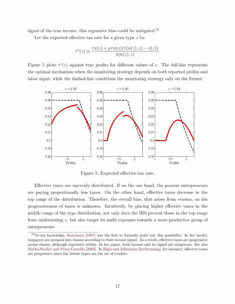
Let the expected effective tax rate for a given type z be

τ e(z) ≡ τx(z) + µτφ(z)(π(n(z), z)− x(z))

π(n(z), z).

Figure 5 plots τ e(z) against true profits for different values of c. The full-line represents

the optimal mechanism when the monitoring strategy depends on both reported profits and

labor input, while the dashed-line conditions the monitoring strategy only on the former.

Figure 5: Expected effective tax rate.

Effective taxes are unevenly distributed. If on the one hand, the poorest entrepreneurs

are paying proportionally less taxes. On the other hand, effective taxes decrease in the

top range of the distribution. Therefore, the overall bias, that arises from evasion, on the

progressiveness of taxes is unknown. Intuitively, by placing higher effective taxes in the

middle range of the type distribution, not only does the IRS prevent those in the top range

from understating z, but also target its audit expenses towards a more productive group of

entrepreneurs.

22To my knowledge, Scotchmer [1987] was the first to formally point out this possibility. In her model,taxpayers are grouped into classes according to their income signal. As a result, effective taxes are progressiveacross classes, although regressive within. In her paper, both income and its signal are exogenous. See alsoMacho-Stadler and Perez-Castrillo [2002]. In Bigio and Zilberman [forthcoming], for instance, effective taxesare progressive since the lowest types are the set of evaders.

17

4.2.3 Outcomes of audits

Once the IRS commits to the cut-off audit rule described in Proposition 1, all audited

taxpayers are known to have reported honestly. This case is depicted in the first plot of

Figure 6, where the thick red line is the optimal monitoring strategy, while the black thin

line is the amount evaded, that is τ(π(n(z), z) − x(z)). Ex-post, audits do not generate

revenue for the government. Hence, the IRS is tempted to deviate from its announced

monitoring strategy and audit the ablest entrepreneurs.

Figure 6: Outcomes of audits, φ(z) vs. τ(π(n(z), z)− x(z)), (c=0.45).

Once the audit rule also depends on n, as in the second plot, audits generate some gross

revenue, but not necessarily positive net revenue. More importantly, audits are not targeting

honest taxpayers anymore. Hence, although there still exists ex-post profitable deviations,

a stronger case for the IRS ability to commit can be made.

Finally, the richest taxpayers are never audited in both mechanisms. However, in con-

trast with the cut-off audit rule, the poorest taxpayers might also not be audited once the

monitoring strategy is conditioned on n.

4.3 Net revenue collection

It is the possibility to set off-equilibrium threats that makes audits a powerful tool to enforce

taxes. As Figure 1 and the second row of Figure 2 illustrate, for any value of c, the reported

income schedule is positive, which translates into a positive lower bound on the net revenue

18

collected.23

However, by conditioning the monitoring strategy on labor, net revenue increases at an

efficiency loss due to distortions imposed almost everywhere. Figure 7 illustrates this trade-

off. The left panel plots net revenue collection as function of the audit cost, ranging from zero

to one. The full-line accounts for a monitoring strategy that depends on both reported profits

and labor input, while the dashed-line considers a monitoring strategy conditioned only on

the former. Finally, the dot-line considers the case in which every entrepreneur is audited

with intensity 1/µ, which ensures truthful income report and efficient employment.24 The

right panel plots the net revenue collection as a fraction of the aggregate product.25 Notice

that, for some values of c, as c decreases, the distortions imposed by policy is high enough

to reduce net revenue collection as a fraction of aggregate product.

Figure 7: Net revenue collection.

23Similarly, when labor is not observable and c becomes arbitrarily large, taxpayers declare the lowest-typeincome (see Proposition 1).

24For c ≤ 1, this is precisely the optimal strategy when the monitoring strategy depends only on employ-ment. Indeed, going through the steps in Bigio and Zilberman [forthcoming], a type z is monitored withintensity 1/µ whenever τπ(n∗(z), z) ≥ c/µ. Hence, since π(n∗(z), z) = 1 ≥ c in this example, all types aremonitored with intensity 1/µ.

25By aggregate product, I mean∫zn(z)αdG(z), which varies with the distortions induced by policy.

19

5 Solution

Given the characterization of (IC) in Lemma 1, the IRS problem is to solve

maxn(z),U(z),φ(z)z

∫ z

z

[π(n(z), z)− U(z)− cφ(z)] dG(z)− Ω

s.t.

(F) φ(z) ≥ 0,∀z ∈ [z, z]

(IR) U(z) ≥ 0,∀z ∈ [z, z]

(LIC)dU

dz(z) = (1− φ(z)µτ)pn(z)α − (1− τ)pn∗(z)α, a.e.,

where Ω =∫ zz

(1− τ)π(n∗(z), z)dG(z).

To solve this problem I ignore (M), φ(z) ≤ 1, n(z) ≥ 0, x(z) ≥ 0, and x(z) ≤ π(n(z), z),

for all z, from the set of constraints. Notice that x(z) ≤ π(n(z), z) is implied by (IR),26

and that φ(z) ≤ 1 never binds in equilibrium.27 The remaining ignored constraints must be

verified in equilibrium.

Let λ be the costate variable associated with the state variable U . The Halmitonian is

H(U, n, φ, λ, z) = [pznα − n− U − cφ]g(z) + λ[(1− φµτ)pnα − (1− τ)pn∗(z)α]. (2)

For a given type z, let ω(z) and θ(z) be the Lagrange multipliers associated with φ(z) ≥ 0

and U(z) ≥ 0, respectively. The Lagrangian is

L(U, n, φ, λ, z) = H(U, n, φ, λ, z) + θU + ωφ.

Let the superscript o denote the optimum solution to the optimization problem stated

above. Following Seierstad and Sydsæter [1987] (Theorem 2, page 361), given that H is

concave in φ, the following set of conditions is sufficient for a global maximum.

1.[z + (1− µτφo(z))λ(z)

g(z)

]αpno(z)α−1 = 1;

2. cg(z) + λ(z)µτpno(z)α = ω(z);

3. dλdz

(z) = g(z)− θ(z);

4. dUo

dz(z) = (1− µτφo(z))pno(z)α − (1− τ)pn∗(z)α;

26Indeed, x(z) ≤ π(n(z), z) if and only if U(z) ≥ (1− τ)[π(n(z), z)− π(n∗(z), z)].27Recall from Section 2 that φ(z) = 1/µ suffices to generate truthful income report and to provide incen-

tives. Since monitoring is costly, φ(z) ≤ 1/µ in equilibrium.

20

5. ω(z) ≥ 0; φo(z) ≥ 0; ω(z)φo(z) = 0;

6. θ(z) ≥ 0; U o(z) ≥ 0; θ(z)U o(z) = 0;

7. λ(z)U o(z) = 0;λ(z) ≤ 0;λ(z)U o(z) = 0;λ(z) ≥ 0;

8. λ(z−) ≥ λ(z+); [λ(z−)− λ(z+)]U o(z) = 0;

9. −λ(z) ≤ zg(z)(1−µτφo(z)) .

1. and 2. are the first order conditions with respect to n and φ, respectively. 3. is

the costate law of motion. 4. is the local incentive compatibility constraint. 5. and 6.

are the complementary slackness conditions that ensure feasibility and individual rationality

respectively. 7. is the set of transversality conditions. 8. needs to be satisfied if the costate

λ is allowed to be discontinuous.28 Finally, 9. guarantees that the Hamiltonian is concave

in n. Notice that 9. can be ignored since it is implied by 1. and φo(z) ≤ 1/µ.

The proof consists of a guess and verify method. The trick is to conjecture the subsets

of the type space [z, z], in which the inequalities U o ≥ 0 and φo ≥ 0 are binding. In other

words, to set the appropriate values for the Lagrange multipliers θ and ω along the interval

[z, z].29

First, note that if the solution is continuously differentiable at the top-type z, then

no(z) = n∗(z), φo(z) = 0, and U o(z) > 0. Moreover, λ(z) = 0, ω(z) > 0 and θ(z) = 0.30

This is a variant of the “non-distortion at the top” kind of result, in which the top-type is

not distorted away from the full-information case, and gets positive informational rent.

By continuity, U o(z) > 0 and ω(z) > 0, which implies θ(z) = 0 and φo(z) = 0, for all

z < z in a small neighborhood of z. Moreover, by solving the differential equation 3. with

boundary λ(z) = 0, one gets λ(z) = G(z) − 1. From 1., no(z) =(αp[z − 1−G(z)

g(z)

]) 11−α

in

this neighborhood.

To proceed with the analysis, I assume one restriction on the distribution of types. Define

h ≡ 1−Gg

, that is one over the hazard rate, and γ ≡ [1− (1− τ)1−αα ] ∈ (0, 1).

28Throughout the paper I use the following notation: h(z−) is the left limit of h at z, h(z+) is the rightlimit of h at z, d−h

dz (z) is the left derivative of h at z, and d+hdz (z) is the right derivative of h at z.

29This strategy is partially inspired by Maggi and Rodrıguez-Clare [1995] analysis of a mechanism designproblem that features a type-dependent participation constraint. However, since this setup is different, themap from this paper to theirs is not perfect. In particular, here, the agent’s objective is not quasi-linearand there are two decision variables. Moreover, for a certain range of values for c, the optimal mechanism isdiscontinuous. See Jullien [2000] for an alternative treatment of type-dependent participation constraints.

30Indeed, from 7., λ(z) ≥ 0. Hence, since c > 0, then ω(z) > 0 (from 2.) and φ(z) = 0 (from 5.). Moreover,no(z) ≥ n∗(z) (from 1.), which implies d−Uo

dz (z) > 0 (from 4.). If by contradiction Uo(z) = 0, then thereexists z < z such that Uo(z) < 0, which violates 6. Hence, Uo(z) > 0, which implies λ(z) = 0 (from 7.),θ(z) = 0 (from 6.), and no(z) = n∗(z) (from 1.).

21

Assumption 1. γz − h(z) is non-decreasing.

This assumption is a weaker version of the monotone hazard rate condition, commonly

assumed in the literature. Indeed, if h(z) is non-increasing then Assumption 1 holds. The

role of this assumption is twofold: first, it ensures that (M) is satisfied without the addi-

tional expositional cost of dealing with bunching; second, it guarantees that the individual

rationality constraints are not violated.

The task, now, is to find a region in the type space, such that either φo(z) ≥ 0 or θ(z) ≥ 0

ceases to hold with equality. Notice that for all z in a small neighborhood of z, both

dU o

dz(z) = p (αp [z − h(z)])

α1−α − (1− τ)p(αpz)

α1−α > 0 (from 4.) (3)

and

cg(z) + λ(z)µτpno(z)α = g(z)[c− h(z)µτp (αp [z − h(z)])

α1−α

]> 0 (from 2.) (4)

hold by continuity. I conjecture that φo(z) ≥ 0 or θ(z) ≥ 0 or both ceases to hold with

equality whenever one of the inequalities in (3) or (4) is strictly reversed. Interestingly, the

solution displays the property that U o(z) = 0 if and only if d−Uo

dz(z) = 0

Formally, define A(z) ≡ γz − h(z),31 which is non-decreasing by Assumption 1, and let

z1 = sups∈[z,z]

A(s) ≤ 0. (5)

The term in curly brackets in equation (5) is obtained from reverting the inequality in (3).

Recall that sups∈[z,z] ∅ = z. By construction, if s ∈ [z, z] : A(s) ≤ 0 is not empty,

Assumption 1 implies that z1 is the highest root that solves A(s) = 0, and that dUo

dz(z) > 0

for all z > z1.

Similarly, define B(z) ≡ h(z)µτp (αp [z − h(z)])α

1−α , and let

z2 = sups∈[z,z]

B(s) > c. (6)

The term in curly brackets in equation (6) is obtained from strictly reverting the inequality

in (4). By construction, if s ∈ [z, z] : B(s) > c is not empty, then B(z2) = c.

In words, analyzing from the right, if z1 ≥ z2, then the differential equation in 4. would

be equalized to zero before conditions 2. and 5. are violated. On the other hand, if z2 > z1,

φ(z) = 0 for some z < z2 would violate conditions 2. and 5. before the differential equation

31Recall that γ ≡ [1− (1− τ)1−αα ] ∈ (0, 1).

22

in 4. is equalized to zero. In particular, I show that for z ≤ maxz1, z2, θ(z) ≥ 0 or

φo(z) ≥ 0 or both cease to hold with equality.

First, consider the case z1 ≥ z2, or equivalently c ≥ maxs∈[z1,z] B(s). The next proposition

studies the case depicted in the forth column in Figure 2, in which c is too high.

Proposition 2. If z1 ≥ z2 (that is, c ≥ maxs∈[z1,z] B(s)), then

no(z) =

(1− τ)

1α (αpz)

11−α if z ≤ z < z1

(αp [z − h(z)])1

1−α if z1 ≤ z ≤ z,

φo(z) = 0 if z ≤ z ≤ z ,

U o(z) =

0 if z ≤ z < z1

p∫ zz1

[(αp [s− h(s)])

α1−α − (1− τ)(αps)

α1−α

]ds if z1 ≤ z ≤ z

,

λ(z) =

−γzg(z) if z ≤ z < z1

G(z)− 1 if z1 ≤ z ≤ z.

Moreover, the solution is continuous.

Proof. For z ≥ z1, the proof is outlined in the text. Hence, if z1 = z the result follows.

Assume z1 > z. For z < z1, set φo(z) = 0, and solve 1. and 4. (equalized to zero) in

no(z) and λ(z). Hence, λ(z) = −γzg(z) and no(z) = (1 − τ)1α (αpz)

11−α . By construction,

λ(z) is continuous, so 8. is satisfied.

Note that Assumption 1 implies that −[γg(z) + g′(z)h(z)] ≤ g(z). From 3. and 6.,

θ(z) = g(z) − dλdz

(z) ≥ 0 is equivalent to −γ[g(z) + zg′(z)] ≤ g(z), which is satisfied if

g(z) + zg′(z) ≥ 0. If g(z) + zg′(z) ≤ 0, which implies that g′(z) < 0, it is enough to show

that −γ[g(z)+zg′(z)] ≤ −[γg(z)+g′(z)h(z)], or equivalently, γz ≤ h(z) for all z ≤ z1, which

follows from z1’s definition. Hence, λ(z) < 0 and U o(z) = 0 are consistent with condition 6.,

the differential equation in 4. equalized to zero, and condition 7.

It remains to show that conditions 2. and 5. hold, that is ω(z) = cg(z)+λ(z)µτp(no(z))α ≥0. In fact, by plugging λ(z) and no(z) into this expression, one obtains γzµτp(1−τ)(αpz)

α1−α ≤

c. Hence, it is enough to show that γz1µτp(1− τ)(αpz1)α

1−α ≤ c. Recalling the definition of

z1, this requirement collapses to B(z1) ≤ c, which follows from z1 ≥ z2.

Finally, it is straightforward to verify that dno

dz(z) ≥ 0, dφo

dz(z) = 0, dxo

dz(z) ≥ 0, whenever

these derivatives exist, and no(z) ≥ 0 and xo(z) ≥ 0. Hence, the omitted constraints are

satisfied.

Consider z2 > z1 instead. Hence, ω(z2) = 0 and d+Uo

dz(z2) > 0. One attempt to solve this

case is to keep λ(z) = G(z)− 1 in a small neighborhood of z2, and for z < z2, let both no(z)

23

and φo(z) jointly solve conditions 1. and 2. (with ω(z) = 0) in this neighborhood. However,

the solution to this system implies that φo(z) < 0 for some z < z2 in any neighborhood

of z2.32 Hence, this approach does not work. To make further progress, λ(z) needs to be

changed for z < z2, and from conditions 3., 7. and 8., it follows that U o(z2) = 0.

Consequently, a natural candidate for the optimal mechanism when z < z2 and z2 > z1

is the solution to the following system of three equations in three unknowns (φ, n and λ).

[g(z)z + (1− µτφ)λ]αpnα−1 − g(z) = 0

cg(z) + λµτpnα = 0 (7)

(1− µτφ)nα − (1− τ)(αpz)α

1−α = 0.

These equations are conditions 1., 2. (with ω = 0), and the differential equation in 4.

equalized to zero. The following assumption guarantees that if a solution exists, it is unique.

Assumption 2. τ ≤ 1−(

2α1+α

) α1−α .

If the tax rate is 25%, any α ≥ 0.22 satisfies this assumption. Similar, if α = 2/3, then it

is satisfied for any τ ≤ 0.36. Therefore, Assumption 2 holds for empirically plausible values

of τ and α. However, if τ > 0.4, this assumption is violated for any value of α.

Note that the derivative of the reservation value with respect to z, (1 − τ)pn∗(z)α, is

decreasing in τ . Therefore, this assumption ensures that countervailing incentives are strong

enough.

The following lemma states sufficient conditions for existence and uniqueness of a solution

to the system in (7).

Lemma 2. For φ ∈ [0, 1/µ] and n ≥ 0:

If c > µτα

[(1− τ)− (1− τ)1α ](αpz)

11−α , then the system of equations in (7) does not have

a solution.

If c ≤ µτα

[(1− τ)− (1− τ)1α ](αpz)

11−α , it has a unique solution.

The proof is in the Appendix. This system might not have a solution for some small

values of z. Define z3 ∈ [0,∞) as being the unique root that solves the following equation

in s.µτ

α[(1− τ)− (1− τ)

1α ](αps)

11−α = c

32Indeed, fix z < z2 in a small neighborhood of z2 such that B(z) > c. By solving condition 2. (withω(z) = 0) at n(z) and using c < B(z), one obtains no(z) < (αp[z − h(z)])

11−α . An inspection of condition 1.

shows that this inequality is true if and only if φo(z) < 0.

24

If z3 < z, redefine z3 = z. Therefore, for all z ∈ [z3, z2), the system in (7) has a unique

solution. Let it be denoted by n(z), φ(z), λ(z)z∈[z3,z2).

The following lemma states some properties this solution has.

Lemma 3. n(z), φ(z), λ(z)z∈[z3,z2) has the following properties:

1. n(z) ∈ [(1− τ)n∗(z), n∗(z)]; φ(z) ∈ [0, 1/µ]; λ(z) < 0;

2. if z3 ∈ (z, z2), then n(z3) = (1−τ)1α (αpz3)

11−α ; φ(z3) = 0; λ(z3) = [(1−τ)

1−αα −1]z3g(z3);

3. dndz

(z) ≥ 0 and dφdz

(z) ≥ 0;

4. n(z) and φ(z) are independent of the distribution of types;

5. (1− µτφ(z))n(z)α = (1− τ)(αpz)α

1−α .

This lemma is proved in the Appendix. The first and second properties state that the

candidate for the optimal mechanism is feasible and continuous at z3 if z3 ∈ (z, z2), respec-

tively. The third and forth properties say that the labor input and auditing probabilities,

that solve (7), are increasing in z, and do not depend on G, although z2 depends. Finally, the

fifth is simply the last equation of the system in (7), which guarantees that (M) is satisfied.

At this degree of generality, it is not possible to characterize closed-form solutions to

n(z), φ(z), λ(z)z∈[z3,z2) for all possible values of α.33 Hence, to proceed with the analysis,

I state a property that this solution might or might not have.

Property 1. For all z ∈ [z3, z2), dλdz

(z) ≤ g(z).

If Property 1 holds, it is possible to characterize the optimal mechanism. This property

is needed to ensure that θ(z) ≥ 0 for all z ∈ [z3, z2), which guarantees that the individual

rationality is satisfied (see conditions 3. and 6.).

The following lemma gives a sufficient condition to ensure that Property 1 holds. Define

ρ ≡ 1+αα

(1− τ)1−αα − 2, and note that ρ ≥ 0 from Assumption 2.

Lemma 4. If γ ≤ ρ+ z g′(z)g(z)

γρ for z ∈ [z3, z2), then Property 1 holds.

The proof is in the Appendix. This sufficient condition imposes a joint restriction on

α, τ , and G. Although not readily interpreted, it can be useful to check if Property 1 is

satisfied. If z follows a uniform distribution, for example, this condition holds if and only if

33If α = 1/2, for example, the system of equations in (7) has a closed-form solution. However, the formulasare too convoluted, since it requires to solve a third degree polynomial equation. Hence, I solve this systemnumerically in Section 4.

25

τ ≤ 1 −(

3α2α+1

) α1−α .34 Notice that even if this condition is violated, Property 1 still can be

attained.

Finally, one last assumption is needed to characterize the optimal mechanism.

Assumption 3. If B(z1) < c then z1 ≥ z2.

Provided that z2 > z1, Assumption 3 guarantees that z3 ≤ z1,35 which is sufficient

to characterize the optimal allocation for z ≤ z3. In particular, for z ≤ z3, the optimal

allocation has the same closed-form as the solution in Proposition 2 for z ≤ z1. Importantly,

this assumption is far from being restrictive. A sufficient condition, for example, is that B(z)

single crosses c.

The cases depicted in the second and third column of Figure 2 illustrate the following

proposition.

Proposition 3. If z2 > z1 (that is, c < maxs∈[z1,z] B(s)) and Property 1 is satisfied, then

no(z) =

(1− τ)

1α (αpz)

11−α if z ≤ z < z3

n(z) if z3 ≤ z < z2

(αp [z − h(z)])1

1−α if z2 ≤ z ≤ z

,

φo(z) =

0 if z ≤ z < z3

φ(z) if z3 ≤ z < z2

0 if z2 ≤ z ≤ z

,

U o(z) =

0 if z ≤ z < z2

p∫ zz2

[(αp [s− h(s)])

α1−α − (1− τ)(αps)

α1−α

]ds if z2 ≤ z ≤ z

,

λ(z) =

−γzg(z) if z ≤ z < z3

λ(z) if z3 ≤ z < z2

G(z)− 1 if z2 ≤ z ≤ z

.

The solution is discontinuous at z = z2. In particular, no(z−2 ) > no(z+2 ), and φo(z−2 ) >

φo(z+2 ) = 0.

The proof is in the Appendix. The next corollary assumes that c→ 0, which is depicted

in the first column of Figure 2.

Corollary 1. If c→ 0, then

no(z), φo(z), U o(z)z → n∗(z), 1/µ, 0z<z ∪ n

∗(z), 0, 0z=z34If α = 1/2, as in Section 4, then any τ ≤ 1/4 ensures that Property 1 is satisfied.35Indeed, assume by contradiction that z3 > z1. Hence, using the definition of z1 and z3, one obtains

B(z1) < c, which implies that z1 ≥ z2.

26

Proof. At c = 0, φ(z) = 1/µ, n(z) = n∗(z), λ(z) = 0, for all z, z2 = z, and z3 = z.

Finally, I also consider τ = 1, which describes a context in which the principal aims to

fully appropriate the agent’s profits. If τ = 1, Assumption 2 is violated, and thus Lemmas

2, 3, and 4, and Proposition 3 are not valid. However, I rely on Property 1 to prove the

following proposition.

Proposition 4. If τ = 1, then

no(z) =

n∗(z) if z ≤ z < z2

(αp [z − h(z)])1

1−α if z2 ≤ z ≤ z,

φo(z) =

1/µ if z ≤ z < z2

0 if z2 ≤ z ≤ z,

U o(z) =

0 if z ≤ z < z2

p∫ zz2

[(αp [s− h(s)])

α1−α − (1− τ)(αps)

α1−α

]ds if z2 ≤ z ≤ z

.

The solution is discontinuous at z = z2. In particular, no(z−2 ) > no(z+2 ) and φo(z−2 ) >

φo(z+2 ) = 0.

Proof. Since τ = 1, z2 ≥ z1. For z ≥ z2, the proof is outlined in the text. If z2 = z, the

result follows. Assume z2 > z. For z < z2, the unique solution of the system of equations in

(7) is φ(z) = 1/µ, n(z) = n∗(z), and λ(z) = −cg(z)/µpn∗(z)α. Since no(z−2 ) > no(z+2 ), then

λ(z−2 ) > λ(z+2 ) and 8. is satisfied. The remaining conditions follow from Property 1 that

implies θ(z) ≥ 0 and U(z) = 0.36

This is the case discussed in Section 4.1.

6 Extensions

To solve the problem, I specify functional forms for five objects: (1) the production technol-

ogy, F (z, n,K) = znα, where K is a vector of other inputs; (2) the utility function, u(y) = y,

where y is income, or equivalently, consumption in a static environment; (3) the penalty func-

tion, M(e) = µe, where e is the amount evaded; (4) the tax schedule, T (x) = τx; and (5)

the audit cost function, C(z, n) = c. In this section, I argue whether these assumptions can

be modified without substantially changing the results.

36In this case, Property 1 implies the following assumption on the distribution of types: g′(z) ≥[1z

α1−α −

µp(αpz)α

1−α

c

]g(z), for all z ≤ z2. In the example, in Section 4, this inequality verifies if and

only if c ≤ 8.

27

6.1 Production technology

In this section, I discuss two possible generalizations for the production technology. First, I

consider a general function of the form zf(n). Second, I show how to extend the model to

accommodate multiple inputs, given that only one is costlessly observable.

6.1.1 General functional form

Recall that Assumptions 1, 2 and 3, which are crucial to prove the results in this paper,

depend on the technological parameter α. Consequently, in order to validate Propositions 2

and 3 under a more general production technology, it is necessary to adapt these assumptions.

Assume, for instance, that the production technology takes the form zf(n), where f ′ > 0,

f ′′ < 0, and f(0) = 0. By applying the solution method developed in Section 5, one can

derive the same qualitative results, but at an expositional cost, as ad-hoc, and somewhat

convoluted, restrictions on f , and its derivatives, would be imposed. It is challenging to

characterize the optimal mechanism when these restrictions are violated.37 Instead, I opt to

explore the Cobb-Douglas case in this paper.

More importantly, although realistic, Assumption 2 restricts the set of values α can take

for a given τ . Therefore, even for the Cobb-Douglas case, the optimal mechanism is not fully

characterized. Before pursuing generalizations for the production technology, it is important

to understand how the optimal mechanism behaves if this assumption is relaxed. Proposition

4 is a small step towards this direction. I leave the characterization of the mechanism when

Assumption 2 is violated as an open question for further research.

6.1.2 Multiple inputs

In this section, I show how the production technology can be generalized to multiple inputs,

as long as only one is costlessly observable by the IRS. Let F (z, n, k1, ..., kI) = znα0∏I

i=1 kαii ,

where kiIi=1 are the inputs that are not observable by the IRS. Assume that F displays

decreasing returns to scale, so∑I

i=0 αi < 1, and αi ≥ 0 for i = 0, .., I. Finally, let ri be the

price of input ki, which is bought in a competitive market.

In the Appendix, given that kiIi=1 are chosen in the second stage of the game, I show

that pre-tax profits can be written as

π(n, z) = ζ(z; p, ri, αi)nα − n, (8)

37For the specific case of Proposition 2, in which c is high enough and φ(z) = 0 for all z, the problem isisomorphic to a standard mechanism design problem with type-dependent reservation value. Jullien [2000]provides a comprehensive characterization of the optimal mechanism for this case.

28

where α = α0/(

1−∑I

i=1 αi

)∈ (0, 1), and ζ is a function of αiIi=1, riIi=1, p, and z.

Consequently, the distribution of z, G, induces a distribution of ζ, say G, and the mechanism

developed above can be applied directly to ζ. However, Assumptions 1 and 3, and Property

1 need to be restated in terms of ζ and G. It is important to keep in mind that, although

pre-tax profits are ζnα − n, the output produced is not ζnα.

This extension is useful in Section 7, where I pursue an empirical evaluation of the

mechanism developed in this paper, for two reasons. First, it accounts for a more realistic

production technology. Second, if z is either log-normally or paretian distributed, which are

commonly assumed in the literature, then also ζ is.

6.2 Audit cost

Without compelling empirical evidence, it is hard to inspect the shape of the audit cost,

C(z, n). It can be argued, for instance, that large firms take longer to monitor than smaller

firms, which justifies ∂C∂n≥ 0. On the other hand, there may be a visibility effect that reduces

the informational cost associated with monitoring larger firms, hence it is also plausible that∂C∂n≤ 0.

Similarly, for a high-ability entrepreneur, it could be easier to circumvent the law, and

hide her income, making ∂C∂z≥ 0. On the other hand, if high-ability translates into more

complex business operations, the need to use of accounting books could make ∂C∂z≤ 0. On

this line, as Kleven et al. [2009] argue, if these books are known to many employees, because

of whistleblowing rewards, the firm is less likely to hide them successfully from the IRS, so∂C∂n∂z≤ 0.

Consequently, I adopt an agnostic view about the audit cost. In particular, I look for

restrictions on its partial derivatives that are sufficient to support the qualitative results

from the previous section.

For simplicity, I assume that the concavity of the Hamiltonian with respect to n is

preserved.38 Hence, from the set of sufficient conditions for an optimum, only items 1. and

2. change.

1′.

[z + (1− µτφo(z))

λ(z)

g(z)

]αpno(z)α−1 = 1 +

∂C

∂n(z, no(z))φ(z)

2′. C(z, no(z))g(z) + λ(z)µτpno(z)α = ω(z)

Note that the definition of z1 does not change, but z2 needs to be redefined.39

38A sufficient condition is ∂2C∂n2 ≥ 0.

39In particular, z2 = sups∈[z,z]B(s) < C(s, (αp[s− h(s)])1

1−α ).

29

It is easy to verify that Proposition 2, which assumes z1 ≥ z2, would still be valid

whenever the LHS of 2′. is greater than or equal to zero for all z ≤ z1. A sufficient condition

for this is

z∂C

∂n(z, no(z))

dno

dz(z) + z

∂C

∂z(z, no(z)) ≤ 1

1− αµτ

αγ(1− τ)(αpz)

11−α .

If z2 ≥ z1, for z ∈ [z3, z2], the optimal mechanism solves the system of equations in

(7). To account for a general audit cost, the first and second equations in (7) need to be

substituted for 1′. and 2′. (with ω(z) = 0). A close inspection of the Appendix, especially

the proofs of Lemmas 2 and 3, reveals that the extra term ∂C∂n

(z, no(z))φ(z) in 1′. complicates

the characterization of the mechanism. Hence, I set ∂C∂n

= 0, and study the case in which the

audit cost C depends only on z. Note that z3 also needs to be redefined.40

Under the additional assumption that zC ′(z) ≤ 11−αC(z), one can follow the steps in

Section 5, and verify that the characterization of the mechanism is qualitatively the same.

Note that this assumption can accommodate a non-monotone audit cost.

If zC ′(z) > 11−αC(z) at some range , the characterization of the mechanism would be

more complicated. Intuitively, if the cost to audit increases at a high rate, the IRS might

prefer to save audits expenses by following a non-monotone monitoring strategy on [z3, z2].

6.3 Tax schedule

By imposing a tax schedule of the form T (x) = τx, I rule out possible interactions between

the progressiveness of the tax system and the optimal monitoring strategy. The simplest

way to introduce progressiveness in the model, without changing the characterization of the

optimal mechanism, is to assume that T (x) = τo + τx, with τo < 0. The only difference,

from the original formulation, is that net revenue collection is increasing on τo.

Consider a general tax schedule T , twice continuous differentiable. In particular, T ′ ∈[0, 1) and T ′′ > 0. For simplicity, I assume that the concavity of the Hamiltonian with

respect to n is preserved. From the set of sufficient conditions for an optimum, the first

order condition with respect to n become[z + (1− µT ′o(z)φo(z))

λ(z)

g(z)

]αpno(z)α−1 = 1 + µTo

′′(z)φo(z)λ(z)

g(z)

[αpzno(z)α−1 − 1

]pno(z)α,

where Ti(z) = T (π(ni(z), z)), T ′i (z) = T ′(π(ni(z), z)), and T ′′i (z) = T ′′(π(ni(z), z)), for

i = o, ∗. Unfortunately, no enters this expression in a convoluted way, jeopardizing any

40In particular, z3 = sups∈[z,z]µτα γ(1− τ)(αps)

11−α < C(s).

30

attempt to extend the analytical results in Proposition 3 for a general tax schedule.

However, if c is high enough, such that φo(z) = 0 for all z, an analogous proposition to

Proposition 2, in which T ′∗(z) plays the role of τ , can be derived. In this case, z1 can be defined

in a similar way, and for z ≤ z1, λ(z) = −γ(z)zg(z), where γ(z) = [1− (1− T ′∗(z))α

1−α ]. The

crucial step is to show that dλdz

(z) ≤ g(z), which is true under the assumptions that T ′ ∈ [0, 1),

T ′′ > 0, and h(z) is non-increasing.

6.4 Penalty and utility functions

Linear penalties and risk neutrality are the hardest assumptions to relax. Consider linear

penalties, for instance. Under the assumption that the penalty function, M , is differentiable,

the local incentive compatibility constraint can be rewritten as

dU

dz(z) = (1− φ(z)M ′(e(z))τ)pn(z)α − (1− τ)pn∗(z)α, a.e.,

where e(z) = τ(π(n(z), z) − x(z)). If M ′(e) depended on e, the IRS problem could not be

rewritten in terms of the informational rents U , since x would still pop out in the Hamil-

tonian. However, this trick substantially facilitates the use of optimal control techniques in

order to solve the problem. A similar argument can be developed for risk neutrality.41

7 A quantitative exploration

The message of this paper is that the IRS can increase net revenue if it is willing to impose

distortions almost everywhere. Hence, in order to inform policy, it is desirable to quantify

this trade-off.

Ideally, one would like to embed the IRS actual practiced monitoring strategy into a

general model, and use data on reported profits, actual profits, inputs, and audits to pin

down the distribution of managerial ability, and the parameters of the model, such as the

audit cost c or the penalty µ. Thus, it would be possible to counterfactually assess the

implications of the mechanism developed in this paper.

However, this approach poses two challenges. First, in most countries, including the

U.S., the audit scheme is strictly guarded or too obscure.42 Hence, it cannot be used as a

41In a standard mechanism design problem, the principal’s objective is usually written in terms of infor-mational rents, instead of compensatory transfers. Consequently, transfers can not pop out in the set oflocal incentive compatibility constraints. This is obtained under the commonly used assumption that utilityis quasi-linear in transfers. In this paper, both linear penalties and risk neutrality allow reported income toplay a similar role to transfers.

42Andreoni et al. [1998] describe how audit policy is conducted in the U.S. for individual income tax

31

benchmark. Second, even in countries where the tax collection agency commits to a publicly

known monitoring strategy, such as in Italy,43 the lack of public data limits this approach.

Hence, in order to provide some assessment on the trade-off between revenue collection

and efficiency, I follow an alternative approach. In particular, I focus on the potential revenue

gains from adopting the optimal mechanism. Let Ro be the revenue collection generated by

the optimal mechanism, and Ra be the actual revenue collected by the U.S. IRS from some

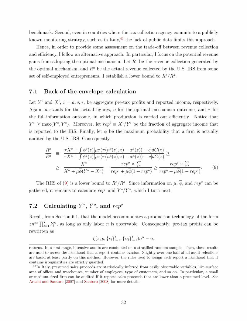
set of self-employed entrepreneurs. I establish a lower bound to Ro/Ra.

7.1 Back-of-the-envelope calculation

Let Y i and X i, i = a, o, ∗, be aggregate pre-tax profits and reported income, respectively.

Again, a stands for the actual figures, o for the optimal mechanism outcome, and ∗ for

the full-information outcome, in which production is carried out efficiently. Notice that

Y ∗ ≥ maxY a, Y o. Moreover, let repi ≡ X i/Y i be the fraction of aggregate income that

is reported to the IRS. Finally, let φ be the maximum probability that a firm is actually

audited by the U.S. IRS. Consequently,

Ro

Ra≡

τXo +∫φo(z)[µτ(π(no(z), z)− xo(z))− c]dG(z)

τXa +∫φa(z)[µτ(π(na(z), z)− xa(z))− c]dG(z)

≥

≥ Xo

Xa + µφ(Y a −Xa)=

repo × Y o

Y a

repa + µφ(1− repa)≥

repo × Y o

Y ∗

repa + µφ(1− repa). (9)

The RHS of (9) is a lower bound to Ro/Ra. Since information on µ, φ, and repa can be

gathered, it remains to calculate repo and Y o/Y ∗, which I turn next.

7.2 Calculating Y ∗, Y o, and repo

Recall, from Section 6.1, that the model accommodates a production technology of the form

znα0∏I

i=1 kαii , as long as only labor n is observable. Consequently, pre-tax profits can be

rewritten as

ζ(z; p, riIi=1, αiIi=1)nα − n,

returns. In a first stage, intensive audits are conducted on a stratified random sample. Then, these resultsare used to assess the likelihood that a report contains evasion. Slightly over one-half of all audit selectionsare based at least partly on this method. However, the rules used to assign each report a likelihood that itcontains irregularities are strictly guarded.

43In Italy, presumed sales proceeds are statistically inferred from easily observable variables, like surfacearea of offices and warehouses, number of employees, type of customers, and so on. In particular, a smallor medium sized firm can be audited if it reports sales proceeds that are lower than a presumed level. SeeArachi and Santoro [2007] and Santoro [2008] for more details.

32

where α = α0/(

1−∑I

i=1 αi

)∈ (0, 1), and ζ is a function of the prices, the technological

parameters, and the managerial ability. Importantly, if z follows a truncated Pareto distri-

bution, which is assumed from now on, also ζ does. Let β be the shape parameter of ζ’s

underlying distribution, which has support [ζ, ζ].

To calculate Y ∗, Y o, and repo, I follow a similar approach to Guner et al. [2008] analysis

of policies that depend on the firm size. In particular, I assume that the U.S. is a “relatively

free-distortion” competitive economy, and use employment data to impose some discipline

on the distribution of managerial ability. By relatively free-distortion, I mean an economy

in which policies do not target the firm size. By competitive, I mean an economy in which

entrepreneurs take prices as given and maximize expected profits. Hence,

n∗(ζ) = (αζ)1

1−α . (10)

Note that distortions that do not target the firm size, such as an input tax, are innocuous.

Indeed, on top of prices, technological parameters, and managerial ability, ζ would also

absorb these distortions.

Importantly, I am implicitly assuming that either the actual monitoring strategy does

not depend on labor input (or any other proxy for the firm size), or entrepreneurs do not

internalize it whenever they take decisions. Although it is likely that the IRS use information

on the business size to select audits, many authors have argued that taxpayers have a poor

knowledge of the audit function. In particular, they tend to overestimate the probability of

an IRS audit. See, for example, Andreoni et al. [1998].

Define η ≡ 1 −∑I

i=0 αi, which is the share of output that goes to the entrepreneur as

pre-tax profits, so α = α0/(α0 + η). By calibrating η, α0, ζ, ζ, and β, I can combine data on

employment at each firm with equation (10) to back out empirically the distribution of ζ, say

G, and then calculate the full-information aggregate profits, Y ∗ ≡∫

[ζn∗(ζ)α − n∗(ζ)]dG(ζ).

To calculate Y o and repo, and thus generate the counterfactual, I make three additional

assumptions. First, I rule out general equilibrium effects through prices, that is I assume p

and riIi=1 are fixed. Second, I assume the distribution of occupations is fixed, such that

entrepreneurs are not allowed to become workers, and vice-versa. Finally, I assume c is high

enough, such that firms are not monitored in equilibrium, and thus the optimal mechanism

is the one derived in Proposition 2.

The first and second assumptions make the distribution of ζ, G, invariant to policy.

Hence, the optimal mechanism can be directly applied to G, which was backed out from

employment data in a previous step.

If the demand for inputs in the corporate sector is relatively large, once compared with

33

the set of firms considered in this exercise, general equilibrium effects trough prices is a minor

issue. Moreover, given prices are fixed and, due to withholding or third-party report, labor

taxes are fully enforced without cost, then the possibility to move across occupations would

further increase net revenue. Indeed, once adopted, the optimal mechanism reduces profits

in entrepreneurial sector. Hence, a standard occupational choice model would predict more

workers fully complying with taxes, and less entrepreneurs managing firms.

The third assumption allows me to calculate the optimal mechanism without specifying

values for the audit cost c and the linear penalty µ. Moreover, by setting a high enough c,

since only labor distortions are used in equilibrium, this assumption underestimate the net

revenue gains from adopting the optimal mechanism.

Consequently, these three assumptions reinforce the aim of this exercise in providing and

lower bound to Ro/Ra.

7.3 Calibration

Following Guner et al. [2008], I set η = 0.2, and α0 = (1− η)× 0.6.

To calibrate ζ, ζ, and β, I use data on employment and entrepreneurship from the 2001

Survey of Consumer Finance (SCF). In particular, I restrict the sample to families, in which

one member actively manages and owns only one business, as in the theory presented above,

and employs at least one worker. I consider only nonfarm sole-proprietors. This procedure

leads to 825 observations.

Table 1 shows some descriptive statistics for the number of workers at each firm.

Mean St. dev. Min Max Obs# workers 6.92 26.68 1 299 825

Table 1: Descriptive statistics (weighted). Source: SCF 2001.

I set ζ = 1.42 and ζ = 7.58, which implies n∗(ζ) = 1 and n∗(ζ) = 299, as in the sample.

Similarly, β = 3.07 generates the average employment per firm in the data. Table 2 shows

that this simple strategy matches reasonably well the firm size distribution observed in the

data.

# workers [0,5) [5,10) [10,20) [20,100) [100,299]Data 80.0% 13.1% 2.9% 2.5% 1.4%

Model 77.1% 10.9% 5.9% 5.2% 1.0%

Table 2: Firm size distribution in data (weighted) and in the model. Source: SCF 2001.

34

Efficient aggregate profits, Y ∗, is 14.4, which is reasonable once wages are the numeraire.

Under the assumptions stated above, to calculate Y o and repo, I need to specify a value for

τ , and then use the formulas from Proposition 2.44

Piketty and Saez [2007] documents that the average federal individual income tax rate

was 11.5% in 2004. If payroll taxes are added, the tax rate increases to 20.8%. Since this

figure ignores both local and state taxes, I generate results for τ ranging from 0.15 to 0.35.

I turn to the choice of µ and φ. According to the U.S. code, title 26,6663, “if any part

of any underpayment of tax required to be shown on a return is due to fraud, there shall be

added to the tax an amount equal to 75 percent of the portion of the underpayment which

is attributable to fraud.” However, typically, penalties are assessed at a rate of 20 percent

of the amount underpaid (Andreoni et al. [1998]).

Similarly, the IRS does not seem to rely on an intensive use of audits to enforce taxes.

Indeed, according to the 2001 IRS Data Book, less than 2% of the schedule C returns were

audited.45 Hence, setting µφ = 0.1 seems a conservative choice, although I also generate

results for µφ ranging from 0.05 to 0.25.46

It is worth mention that if non-pecuniary penalties, such as the possibility of impris-

onment, were properly accounted for in the model, Ro/Ra would increase even more. The

same argument is valid for other types of cost, such as the financial cost of hiring professional

assistance or the moral cost of being an outlaw.

Finally, following Slemrod [2007], I set repa = 0.43, which is the fraction of nonfarm

sole-proprietor income that is reported to the IRS in 2001. This figure is provided by

the IRS, which combines information from a program of random intensive audits, ongoing

enforcement activities, and other special studies about particular sources of income (such as

cash earnings) that is unlikely to be uncover even in an intensive audit. Alternatively, I also

generate results for repa = 0.65, which is estimated by Feldman and Slemrod [2007] using

unaudited tax returns data for 1999 in the U.S. Under the assumption that charity donations

are unrelated to the source of income, these authors adapt the econometric approach in

Pissarides and Weber [1989] to estimate self-employment income underreporting.47

44Given the values chosen for the parameters, the truncated Pareto distribution does not satisfy Assump-tion 1. However, for the purpose of this empirical exercise, an inspection of the proof of Proposition 2 revealsthat this assumption can be relaxed as follows: 1. z−h(z) is non-decreasing for z ≥ z1; 2. γz−h(z) ≤ 0 forz ≤ z1; and 3. −γ[g(z) + zg′(z)] ≤ g(z) for z ≤ z1. These properties are satisfied in this section.

45Schedule C returns are those filled by nonfarm self-employed.46Even if some taxpayers face high probabilities of being audited, by plugging a smaller value for φ, it is

still likely that the inequality in (9) is satisfied, especially if these taxpayers represent a small fraction of thepopulation.

47In their original approach, Pissarides and Weber [1989] assume that food consumption, instead of charitydonations, is unrelated to the source of income. These authors estimate that income underreporting forBritish self-employed was approximately 35% in 1982.

35

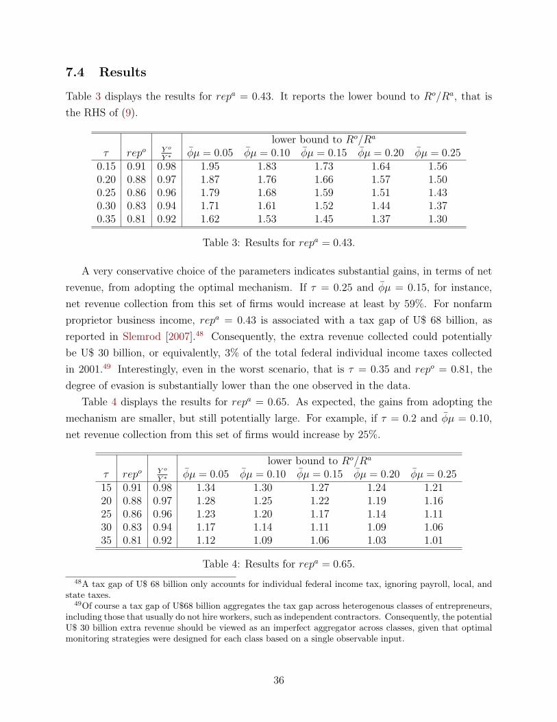
7.4 Results

Table 3 displays the results for repa = 0.43. It reports the lower bound to Ro/Ra, that is

the RHS of (9).

lower bound to Ro/Ra

τ repo Y o

Y ∗φµ = 0.05 φµ = 0.10 φµ = 0.15 φµ = 0.20 φµ = 0.25

0.15 0.91 0.98 1.95 1.83 1.73 1.64 1.560.20 0.88 0.97 1.87 1.76 1.66 1.57 1.500.25 0.86 0.96 1.79 1.68 1.59 1.51 1.430.30 0.83 0.94 1.71 1.61 1.52 1.44 1.370.35 0.81 0.92 1.62 1.53 1.45 1.37 1.30

Table 3: Results for repa = 0.43.

A very conservative choice of the parameters indicates substantial gains, in terms of net

revenue, from adopting the optimal mechanism. If τ = 0.25 and φµ = 0.15, for instance,

net revenue collection from this set of firms would increase at least by 59%. For nonfarm

proprietor business income, repa = 0.43 is associated with a tax gap of U$ 68 billion, as

reported in Slemrod [2007].48 Consequently, the extra revenue collected could potentially

be U$ 30 billion, or equivalently, 3% of the total federal individual income taxes collected

in 2001.49 Interestingly, even in the worst scenario, that is τ = 0.35 and repo = 0.81, the

degree of evasion is substantially lower than the one observed in the data.

Table 4 displays the results for repa = 0.65. As expected, the gains from adopting the

mechanism are smaller, but still potentially large. For example, if τ = 0.2 and φµ = 0.10,

net revenue collection from this set of firms would increase by 25%.

lower bound to Ro/Ra

τ repo Y o

Y ∗φµ = 0.05 φµ = 0.10 φµ = 0.15 φµ = 0.20 φµ = 0.25

15 0.91 0.98 1.34 1.30 1.27 1.24 1.2120 0.88 0.97 1.28 1.25 1.22 1.19 1.1625 0.86 0.96 1.23 1.20 1.17 1.14 1.1130 0.83 0.94 1.17 1.14 1.11 1.09 1.0635 0.81 0.92 1.12 1.09 1.06 1.03 1.01

Table 4: Results for repa = 0.65.

48A tax gap of U$ 68 billion only accounts for individual federal income tax, ignoring payroll, local, andstate taxes.

49Of course a tax gap of U$68 billion aggregates the tax gap across heterogenous classes of entrepreneurs,including those that usually do not hire workers, such as independent contractors. Consequently, the potentialU$ 30 billion extra revenue should be viewed as an imperfect aggregator across classes, given that optimalmonitoring strategies were designed for each class based on a single observable input.

36

In the Appendix, I do some sensitivity analysis. In particular, I vary both β and α.

Results are remarkably robust to variations of β, but net revenue collected would increase

even more for higher values of α.

Leaving aside explanations based on moral, psychological, or social reasonings, the dis-

crepancy between the model and the data highlights the inability of the IRS to deter evasion

trough audits. In particular, given that in the U.S., the IRS strategy to select audits is

strictly guarded, these results suggest that the IRS can substantially fight evasion, and thus

increase revenue collection, by committing to an optimal monitoring strategy that depends

on proxies for the business size. Recall that this exercise assumes that c is high enough, such

that in equilibrium, φo(z) = 0 for all z, and thus these results do not rely on an abusive use

of audits, which is consistent with the IRS actual practices.

The adoption of such rule raises other issues, such as the distortions it imposes almost

everywhere, or its implications for horizontal equity. From an ethical point o view, it would

be questionable an IRS behavior that not only tolerates, but also explicitly induces evasion.

Of course this exercise is somewhat limited, as general equilibrium and occupational

choice effects are ruled out, and the assumption that policies do not target firm size might not

be the right benchmark. Moreover, non-linearities on the tax schedule have implications for

both the optimal mechanism, and the actual revenue collected by the U.S. IRS. Nonetheless,

this exercise provides a first assessment on the potential gains from optimally conditioning

the monitoring strategy on employment.

8 Conclusion

The relevance of the theory presented in this paper hinges on the plausibility of two assump-

tions. First, employment at each firm is easily observable by the IRS. Second, audits are

relevant to explain self-employed income tax evasion.

At least in developed countries, to a first approximation, there is empirical evidence

suggesting that labor is readily available information to the IRS. In particular, only 1 percent

of wages and salaries are not reported to the IRS in the U.S. (Slemrod [2007]), and even less

in Denmark (Kleven et al. [2010]). If income taxes are subject to third-party report, as in

the case of employers withholding wage taxes, it is unlikely that the parties involved would

collude to evade taxes.50 Moreover, as long as wages are partially declared, the IRS still

has information about the employee and the firm for which she works.51 Even if unskilled

50In the U.S., for instance, firms issue W-2 forms, one for each worker, detailing her identity and theamount of wages paid. Each form is sent to the IRS and the relevant employee. The latter uses the W-2form to file her income tax return. See Logue and Slemrod [2009] for more details.

51In particular, a computer program that matches reports from both workers and firms is enough. Hence,

37

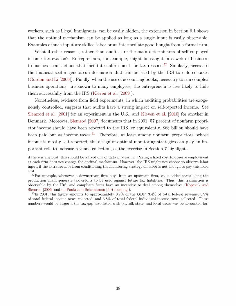
workers, such as illegal immigrants, can be easily hidden, the extension in Section 6.1 shows

that the optimal mechanism can be applied as long as a single input is easily observable.

Examples of such input are skilled labor or an intermediate good bought from a formal firm.

What if other reasons, rather than audits, are the main determinants of self-employed

income tax evasion? Entrepreneurs, for example, might be caught in a web of business-

to-business transactions that facilitate enforcement for tax reasons.52 Similarly, access to

the financial sector generates information that can be used by the IRS to enforce taxes

(Gordon and Li [2009]). Finally, when the use of accounting books, necessary to run complex

business operations, are known to many employees, the entrepreneur is less likely to hide

them successfully from the IRS (Kleven et al. [2009]).

Nonetheless, evidence from field experiments, in which auditing probabilities are exoge-

nously controlled, suggests that audits have a strong impact on self-reported income. See

Slemrod et al. [2001] for an experiment in the U.S., and Kleven et al. [2010] for another in

Denmark. Moreover, Slemrod [2007] documents that in 2001, 57 percent of nonfarm propri-

etor income should have been reported to the IRS, or equivalently, $68 billion should have

been paid out as income taxes.53 Therefore, at least among nonfarm proprietors, whose

income is mostly self-reported, the design of optimal monitoring strategies can play an im-

portant role to increase revenue collection, as the exercise in Section 7 highlights.

if there is any cost, this should be a fixed one of data processing. Paying a fixed cost to observe employmentat each firm does not change the optimal mechanism. However, the IRS might not choose to observe laborinput, if the extra revenue from conditioning the monitoring strategy on labor is not enough to pay this fixedcost.

52For example, whenever a downstream firm buys from an upstream firm, value-added taxes along theproduction chain generate tax credits to be used against future tax liabilities. Thus, this transaction isobservable by the IRS, and compliant firms have an incentive to deal among themselves (Kopczuk andSlemrod [2006] and de Paula and Scheinkman [forthcoming]).

53In 2001, this figure amounts to approximately 0.7% of the GDP, 3.4% of total federal revenue, 5.9%of total federal income taxes collected, and 6.8% of total federal individual income taxes collected. Thesenumbers would be larger if the tax gap associated with payroll, state, and local taxes was be accounted for.

38

A Proofs

The following proofs involve a change of variables that reduces the number of equations in

(7). Define Φ ≡ 1− µτφ and N ≡ nα. Using the first and the second equations to eliminate

λ from the problem, one reaches the following system of two equations in two unknowns (Φ

and N).

Φ =µτ

αc

[αpzN −N

1α

](11)

Φ =(1− τ)[αpz]

α1−α

N

Moreover, φ ∈ [0, 1/µ] implies that Φ ∈ [1− τ, 1].

Let Φ1(N) = µταc

[αpzN − N 1α ], Φ2(N) = (1−τ)(αpz)

α1−α

N, and define N∗ ≡ (αpz)

α1−α . Since

Φ2 is strictly decreasing, then any solution to this system implies that N ∈ [(1− τ)N∗, N∗].

A.1 Proof of Lemma 2

Notice that Φ1 is strictly concave, and Φ2 is strictly convex. Therefore, Φ1 = Φ2 at most

at two values of N . Moreover, Φ1(N∗) = 0 < (1 − τ) = Φ2(N∗), thus this system has one

solution if Φ1((1− τ)N∗) > Φ2((1− τ)N∗) = 1. A little algebra shows that this requirement

holds if and only if c < µτα

[(1− τ)− (1− τ)1α ](αpz)

11−α .

This system does not have a solution if and only if Φ1(N) < Φ2(N) for all N ∈ [(1 −τ)N∗, N∗]. Note that Φ1(N) < Φ2(N) if and only if

µτ [αpzN2 −N 1+αα ]

α(1− τ)(αpz)α

1−α< c

Taking the first order condition of the LHS with respect to N , one gets N =(2 α

1+ααpz

) α1−α .

But Assumption 2 implies that N ≤ (1 − τ)N∗. Hence, there are two possible candidates

for a maximum: (1− τ)N∗ and N∗. Plugging them into the LHS, and choosing the one that

yields the highest value, one concludes that this system does not have a solution if and only

if µτα

[(1− τ)− (1− τ)1α ](αpz)

11−α < c.

Finally, when c = µτα

[(1− τ)− (1− τ)1α ](αpz)

11−α , N = (1− τ)N∗ and Φ = 1 is the only

solution to the system of equations above.

39

A.2 Proof of Lemma 3

Items 1., 4. and 5. are immediate. Item 2. follows from the fact that c = µτα

[(1− τ)− (1−τ)

1α ](αpz3)

11−α , thus N(z3) = (1 − τ)N∗(z3) and Φ(z3) = 1. It remains to show 3., that is

dNdz≥ 0 and dΦ

dz≤ 0.

Equalizing both equations in (11), one obtains

αpzN2 −N1+αα =

αc

µτ(1− τ)(αpz)

α1−α .

Differentiating it with respect to N and z leads to

dN

dz=

(1− τ)αcµτ

α1−α

(αpz)α

1−α

z− αpN2

αpz2N − 1+ααN

1α

.

For dNdz≥ 0, it is enough to show that both the denominator and the numerator are negative.

Indeed, the numerator is smaller then zero if and only if

(1− τ)αc

µτ

α

1− α(αpz)

α1−α

z− αpN2 < 0.

Therefore, by plugging the smallest possible value for N , (1− τ)N∗, and after some manip-

ulations,

c <1− αα

(1− τ)µτ

α(αpz)

11−α .

Since c ≤ µτα

[(1− τ)− (1− τ)1α ](αpz)

11−α , it is enough to show that

1− (1− τ)1−αα <

1− αα

,

which follows from Assumption 2.

The denominator is smaller then zero if and only if

αpz2N − 1 + α

αN

1α ≤ 0 ⇐⇒ αpz2

α

1 + α≤ N

1−αα .

Hence, it is enough to plug the smallest possible value for N , (1− τ)N∗, into this inequality,

and check that it holds. Indeed,

2α

1 + α≤ (1− τ)

1−αα

is true by Assumption 2.

40

Similarly, from (11),

Φ =µτ

αc

[(1− τ)

(αpz)1

1−α

Φ− (1− τ)

1α

(αpz)1

1−α

Φ1α

]

Differentiating it with respect to Φ and z, and after some manipulation, leads to

dΦ

dz=

(1− τ)µταc

11−α

(αpz)1

1−α

z

[Φ

1−αα − (1− τ)

1−αα

]1+αα

Φ1α − µτ

αc(1− τ)(αpz)

11−α 1−α

αΦ

1α−2

.

Therefore, given Φ ≥ (1− τ), for dΦdz≤ 0, it is enough to show that the denominator of the

previous equation is negative. That is,

1 + α

αΦ

1α − µτ

αc(1− τ)(αpz)

11−α

1− αα

Φ1α−2 ≤ 0 ⇐⇒ c ≤ µτ

α(1− τ)(αpz)

11−α

1− α1 + α

Φ−2

Since c ≤ µτα

[(1− τ)− (1− τ)1α ](αpz)

11−α , it is enough to show that

1− (1− τ)1−αα ≤ 1− α

1 + α,

which follows from Assumption 2.

A.3 Proof of Lemma 4

Notice that λ(z) = − cg(z)µτpN(z)

. Taking derivatives and reorganizing the terms, one obtains

dλ

dz(z) =

1

N(z)

c

µτp

[N ′(z)

N(z)g(z)− g′(z)

],

If N′(z)

N(z)g(z)−g′(z) ≤ 0, then the assertion is trivial. On the other hand, if N

′(z)N(z)

g(z)−g′(z) > 0,

dλ

dz(z) ≤ z

N(z)[(1− τ)− (1− τ)

1α ](αpz)

α1−α

[N ′(z)

N(z)g(z)− g′(z)

]≤ (12)

≤ γ

[N ′(z)

N(z)zg(z)− zg′(z)

],

where the first inequality follows from c ≤ µτα

[(1− τ)− (1− τ)1α ](αpz)

11−α for all z ∈ [z3, z2),

while the second follows from N(z) ∈ [(1− τ)N∗, N∗] for all z ∈ [z3, z2).54

54Recall that γ ≡ 1− (1− τ)1−αα .

41

Note that

zN ′(z)

N(z)=

αpzN(z)− (1− τ)αcµτ

α1−α(αpz)

α1−α 1

N(z)

1+ααN(z)

1α − 2αpzN(z)

< (13)

<αpz

1+ααN(z)

1−αα − 2αpz

≤ 11+αα

(1− τ)1−αα − 2

=1

ρ.

Consequently, by plugging (13) into (12), it is straightforward to verify that

γ ≤ ρ+ zg′(z)

g(z)γρ⇒ dλ

dz(z) ≤ g(z).

A.4 Proof of Proposition 3

For z ≥ z2, the proof is outlined in the text. Hence, if z2 = z, the result follows. Assume

z2 > z. For z ∈ [z3, z2), set φo(z) = φ(z), no(z) = n(z), and λo(z) = λ(z), which satisfy

conditions 1., 2., and 5. Moreover, Property 1 and condition 3. imply θ(z) ≥ 0, thus from

6., I set U(z) = 0, which agrees with the differential equation in 4. equalized to zero, given

U(z3) = 0 is the boundary condition. If z3 = z, since λ(z3) < 0, condition 7. is satisfied.

It remains to show that 8. is satisfied. Note that at z = z2, both conditions 1. and 2.

(with ω = 0) hold with equality, but 0 = d−Uo

dz(z2) < d+Uo

dz(z2). Hence, at z = z2, no(z) and

φo(z) are discontinuous.

If the domain of N and Φ are extended to [0, N∗] and [1−τ,∞), respectively, by following

similar steps to the ones in the proof of Lemma 2, one can verify that this system has always

two solutions if 0 < c < µτα

[(1 − τ) − (1 − τ)1−αα ](αpz)

11−α . Index these solutions by l and

h. At z = z2 , it is easy to verify that, without lost of generality, nl(z2) < no(z−2 ) < nh(z2),

φl(z2) < φo(z−2 ) < φh(z2), and λl(z2) < λ(z−2 ) < λh(z2). By restricting the domain of N and

Φ to be between [(1 − τ)N∗, N∗], and [(1 − τ), 1], respectively, the solution indexed by l is

lost. Consequently, 8. is satisfied.

Finally, for z < z3, given that z3 > z, the proof is similar to the one in Proposition 2

provided that Assumption 3 implies that z3 ≤ z1.

A.5 Working out equation (8)

If F (z, n, k1, ..., kI) = znα0∏I

i=1 kαii , expected profits are

pznα0

I∏i=1

kαii − n−I∑i=1

riki − τx− µτϕ(n, x)

(pznα0

I∏i=1

kαii − n−I∑i=1

riki − x

), (14)

42

By taking the first order condition of (14) with respect to kI , which is chosen in the last

stage of the game, one obtains

kI =

(αIrIpznα0

I−1∏i=1

kαii

) 11−αI

.

By plugging it back to (14), expected profits can be rewritten as

ζ(z; p, rI , αI)nαo

I−1∏i=1

kαii −n−I−1∑i=1

riki−τx−µτϕ(n, x)

(ζ(z; p, rI , αI)n

αo

I−1∏i=1

kαii − n−I−1∑i=1

riki − x

),

where αi = αi1−αI

, and ζ(z; p, rI , αI) =

[(αIrI

) αI1−αI − rI

(1rI

) αI1−αI

](pz)

αI1−αI

Proceeding iteratively, one reaches (8). Moreover, if z is either log-normally or paretian

distributed, then also ζ is.

43

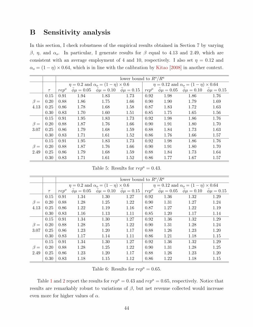
B Sensitivity analysis

In this section, I check robustness of the empirical results obtained in Section 7 by varying

β, η, and αo. In particular, I generate results for β equal to 4.13 and 2.49, which are

consistent with an average employment of 4 and 10, respectively. I also set η = 0.12 and

αo = (1− η)× 0.64, which is in line with the calibration by Kitao [2008] in another context.

lower bound to Ro/Ra

η = 0.2 and αo = (1− η)× 0.6 η = 0.12 and αo = (1− η)× 0.64τ repo φµ = 0.05 φµ = 0.10 φµ = 0.15 repo φµ = 0.05 φµ = 0.10 φµ = 0.15

0.15 0.91 1.94 1.83 1.73 0.92 1.98 1.86 1.76β = 0.20 0.88 1.86 1.75 1.66 0.90 1.90 1.79 1.694.13 0.25 0.86 1.78 1.68 1.58 0.87 1.83 1.72 1.63

0.30 0.83 1.70 1.60 1.51 0.85 1.75 1.65 1.560.15 0.91 1.95 1.83 1.73 0.92 1.98 1.86 1.76

β = 0.20 0.88 1.87 1.76 1.66 0.90 1.91 1.80 1.703.07 0.25 0.86 1.79 1.68 1.59 0.88 1.84 1.73 1.63

0.30 0.83 1.71 1.61 1.52 0.86 1.76 1.66 1.570.15 0.91 1.95 1.83 1.73 0.92 1.98 1.86 1.76

β = 0.20 0.88 1.87 1.76 1.66 0.90 1.91 1.80 1.702.49 0.25 0.86 1.79 1.68 1.59 0.88 1.84 1.73 1.64

0.30 0.83 1.71 1.61 1.52 0.86 1.77 1.67 1.57

Table 5: Results for repa = 0.43.

lower bound to Ro/Ra

η = 0.2 and αo = (1− η)× 0.6 η = 0.12 and αo = (1− η)× 0.64τ repo φµ = 0.05 φµ = 0.10 φµ = 0.15 repo φµ = 0.05 φµ = 0.10 φµ = 0.15

0.15 0.91 1.34 1.30 1.27 0.92 1.36 1.32 1.29β = 0.20 0.88 1.28 1.25 1.22 0.90 1.31 1.27 1.244.13 0.25 0.86 1.22 1.19 1.16 0.87 1.27 1.22 1.19

0.30 0.83 1.16 1.13 1.11 0.85 1.20 1.17 1.140.15 0.91 1.34 1.30 1.27 0.92 1.36 1.32 1.29

β = 0.20 0.88 1.28 1.25 1.22 0.90 1.31 1.28 1.243.07 0.25 0.86 1.23 1.20 1.17 0.88 1.26 1.23 1.20

0.30 0.83 1.17 1.14 1.11 0.86 1.21 1.18 1.150.15 0.91 1.34 1.30 1.27 0.92 1.36 1.32 1.29

β = 0.20 0.88 1.28 1.25 1.22 0.90 1.31 1.28 1.252.49 0.25 0.86 1.23 1.20 1.17 0.88 1.26 1.23 1.20

0.30 0.83 1.18 1.15 1.12 0.86 1.22 1.18 1.15

Table 6: Results for repa = 0.65.

Table 1 and 2 report the results for repa = 0.43 and repa = 0.65, respectively. Notice that

results are remarkably robust to variations of β, but net revenue collected would increase

even more for higher values of α.

44

References

M. G. Allingham and A. Sandmo. Income tax evasion: A theoretical analysis. Journal of

Public Economics, 1(3-4):323–338, November 1972. 2

J. Andreoni, B. Erard, and J. Feinstein. Tax compliance. Journal of Economic Literature,

36(2):818–860, June 1998. 2, 6, 31, 33, 35

G. Arachi and A. Santoro. Tax enforcement for smes: Lessons from the italian experience?

eJournal of Tax Research, 5(2):225–243, 2007. 32

R. Armenter and T. M. Mertens. Fraud deterrence in dynamic mirrleesian economies. FRB

of Philadelphia Working Paper No. 10-7, 2010. 2

M. Bassetto and C. Phelan. Tax riots. Review of Economic Studies, 75(3):649–669, July

2008. 2

G. S. Becker. Crime and punishment: An economic approach. Journal of Political Economy,

76(2):169–217, March/April 1968. 2

S. Bigio and E. Zilberman. Optimal self-employment income tax enforcement. Journal of

Public Economics, forthcoming. 2, 9, 10, 11, 17, 19

K. C. Border and J. Sobel. Samurai accountant: A theory of auditing and plunder. Review

of Economic Studies, 54(4):525–540, October 1987. 2

P. Chander and L. L. Wilde. General characterization of optimal income tax enforcement.

Review of Economic Studies, 65(1):165–183, January 1998. 2

H. Cremer and F. Gahvari. Tax evasion and the general income tax. Journal of Public

Economics, 60(2):235–249, May 1996. 2

H. Cremer, M. Marchand, and P. Pestieau. Evading, auditing and taxing: The equity-

compliance tradeoff. Journal of Public Economics, 43(1):67–92, October 1990. 2

A. de Paula and J. A. Scheinkman. Value added taxes, chain effects and informality. Amer-

ican Economic Journal: Macroeconomics, forthcoming. 38

B. Erard and J. Feinstein. Honesty and evasion in the tax compliance game. Rand Journal

of Economics, 25(1):1–19, Spring 1994. 6

N. E. Feldman and J. Slemrod. Estimating tax noncompliance with evidence from unaudited

tax returns. Economic Journal, 117(518):327–352, March 2007. 35

45

D. Fudenberg and J. Tirole. Game Theory. MIT Press, 1991. 10

R. Gordon and W. Li. Tax structures in developing countries: Many puzzles and a possible

explanation. Journal of Public Economics, 93(7-8):855–866, August 2009. 38

N. Guner, G. Ventura, and Y. Xu. Macroeconomic implications of size-dependent policies.

Review of Economic Dynamics, 11(4):721–744, October 2008. 33, 34

B. Jullien. Participation constraints in adverse selection models. Journal of Economic

Theory, 93(1):1–47, July 2000. 21, 28

S. Kitao. Entrepreneurship, taxation and capital investment. Review of Economic Dynamics,

11(1):44–69, January 2008. 44

H. J. Kleven, C. T. Kreiner, and E. Saez. Why can modern governments tax so much? an

agency model of firms as fiscal intermediaries. NBER Working Paper 15218, 2009. 29, 38

H. J. Kleven, M. B. Knudsen, C. T. Kreiner, S. Pedersen, and E. Saez. Unwilling or unable

to cheat? evidence from a randomized tax audit experiment in denmark. NBER Working

Paper 15769, 2010. 2, 37, 38

W. Kopczuk and J. Slemrod. Putting firms into optimal tax theory. American Economic

Review Papers and Proceedings, 96(2):130–134, May 2006. 38

T. R. Lewis and D. E. M. Sappington. Countervailing incentives in agency problems. Journal

of Economic Theory, 49(2):294–313, December 1989. 9

K. D. Logue and J. Slemrod. Of coase, calabresi, and optimal tax liability. John M. Olin

Center for Law & Economics Working Paper 96, 2009. 37

I. Macho-Stadler and J. D. Perez-Castrillo. Audting with signals. Economica, 69(273):1–20,

February 2002. 17

I. Macho-Stadler and J. D. Perez-Castrillo. Optimal auditing with heteregeneous income

sources. International Economic Review, 38(4):951–968, November 1997. 2

G. Maggi and A. Rodrıguez-Clare. On countervailing incentives. Journal of Economic

Theory, 66(1):238–263, June 1995. 21

D. Mookherjee and I. Png. Optimal auditing, insurance, and redistribution. Quarterly

Journal of Economics, 104(2):399–415, May 1989. 2, 11

46

S. C. Parker. Entrepreneurial growth and dynamic tax evasion incentives. Working Paper,

2010. 2

T. Piketty and E. Saez. How progressive is the u.s. federal tax system? a historical and

international perspective. Journal of Economic Perspectives, 21(1):3–24, Winter 2007. 35

C. A. Pissarides and G. Weber. An expenditure-based estimate of britain’s black economy.

Journal of Public Economics, 39(1):17–32, June 1989. 35

A. M. Polinsky and S. Shavell. The economic theory of public enforcement of law. Journal

of Economic Literature, 38(1):45–76, March 2000. 6

B. Ravikumar and Y. Zhang. Optimal auditing in a dynamic model of tax compliance.

Working Paper, 2010. 2

J. F. Reinganum and L. L. Wilde. Income tax compliance in a principal-agent framework.

Journal of Public Economics, 26(1):1–18, February 1985. 2

H. S. Rosen. Public Finance. McGraw-Hill, 2005. 6

I. Sanchez and J. Sobel. Hierarchical design and enforcement income tax policies. Journal

of Public Economics, 50(3):345–369, March 1993. 2, 3, 9, 11, 16

A. Sandmo. The theory of tax evasion: A retrospective view. National Tax Journal, 58(4):

643–663, December 2005. 2

A. Santoro. Taxpayer’s choices under studi di settore: What do we know and how we can

interpret it? Giornale degli Economisti e Annali di Economia, 67(2):161–184, July 2008.

32

S. Scotchmer. Audit classes and tax enforcement policy. American Economic Review Papers

and Proceedings, 77(2):229–233, May 1987. 17

A. Seierstad and K. Sydsæter. Optimal Control Theory with Economic Applications. North-

Holland, 1987. 20

J. Slemrod. Cheating ourselves: The economics of tax evasion. Journal of Economic Per-

spectives, 21(1):25–48, Winter 2007. 2, 5, 35, 36, 37, 38

J. Slemrod and S. Yitzhaki. Tax avoidance, evasion and administration. In A. J. Auerbach

and M. Feldstein, editors, Handbook of Public Economics, volume 3, chapter 22, pages

1423–1470. Elsevier B.V., 2002. 2

47

J. Slemrod, M. Blumenthal, and C. Christian. Taxpayer response to an increased proba-

bility of audit: Evidence from a controlled experiment in minnesota. Journal of Public

Economics, 79(3):455–483, March 2001. 38

R. M. Townsend. Optimal contracts and competitive markets with costly state verification.

Journal of Economic Theory, 21(2):265–293, October 1979. 2

48