audio waveform - recordingologyrecordingology.com/.../soundfx_ch01_audiowaveform.pdfsound fx...

Audio Waveform 1

“Catch a waveand you’re sittin’ on top of the world.” — “CATCH A WAVE,” THE BEACH BOYS, SURFER GIRL (CAPITAL RECORDS, 1963)

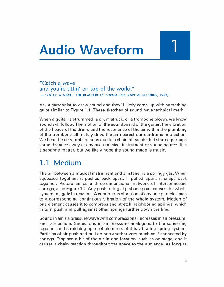
Ask a cartoonist to draw sound and they’ll likely come up with something quite similar to Figure 1.1. These sketches of sound have technical merit.

When a guitar is strummed, a drum struck, or a trombone blown, we know sound will follow. The motion of the soundboard of the guitar, the vibration of the heads of the drum, and the resonance of the air within the plumbing of the trombone ultimately drive the air nearest our eardrums into action. We hear the air vibrate near us due to a chain of events that started perhaps some distance away at any such musical instrument or sound source. It is a separate matter, but we likely hope the sound made is music.

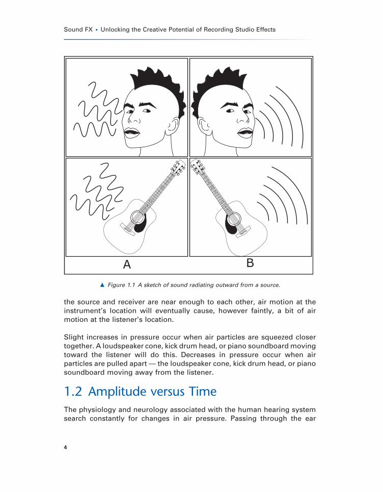
1.1 MediumThe air between a musical instrument and a listener is a springy gas. When squeezed together, it pushes back apart. If pulled apart, it snaps back together. Picture air as a three-dimensional network of interconnected springs, as in Figure 1.2. Any push or tug at just one point causes the whole system to jiggle in reaction. A continuous vibration of any one particle leads to a corresponding continuous vibration of the whole system. Motion of one element causes it to compress and stretch neighboring springs, which in turn push and pull against other springs further down the line.

Sound in air is a pressure wave with compressions (increases in air pressure) and rarefactions (reductions in air pressure) analogous to the squeezing together and stretching apart of elements of this vibrating spring system. Particles of air push and pull on one another very much as if connected by springs. Displace a bit of the air in one location, such as on-stage, and it causes a chain reaction throughout the space to the audience. As long as

3

Ch001-K52032.indd 3Ch001-K52032.indd 3 5/30/2007 10:27:13 AM5/30/2007 10:27:13 AM

Sound FX � Unlocking the Creative Potential of Recording Studio Effects

4

the source and receiver are near enough to each other, air motion at the instrument’s location will eventually cause, however faintly, a bit of air motion at the listener’s location.

Slight increases in pressure occur when air particles are squeezed closer together. A loudspeaker cone, kick drum head, or piano soundboard moving toward the listener will do this. Decreases in pressure occur when air particles are pulled apart — the loudspeaker cone, kick drum head, or piano soundboard moving away from the listener.

1.2 Amplitude versus TimeThe physiology and neurology associated with the human hearing system search constantly for changes in air pressure. Passing through the ear

� Figure 1.1 A sketch of sound radiating outward from a source.


Chapter 1 � Audio Waveform

5

canal, changes in sound pressure push and pull on the ear drum, triggering a chain reaction that ultimately leads to the perception of sound. The pressure of a sound wave is the same type of air pressure associated with pumping air into a tire: PSI (pounds per square inch) in the some parts of the world, or kPa (kilopascals) elsewhere. Micropascals (µPa) is the preferred order-of-magnitude expression of air pressure for sound that humans can healthily hear.

A common way to graph sound plots air pressure as the vertical axis and time as the horizontal axis. Such a graph describes sound at a single, fi xed location in space. As sound occurs, the air pressure at that point increases and decreases several times per second. The familiar plots of sound, in textbooks and comic books, accurately portray this concept.

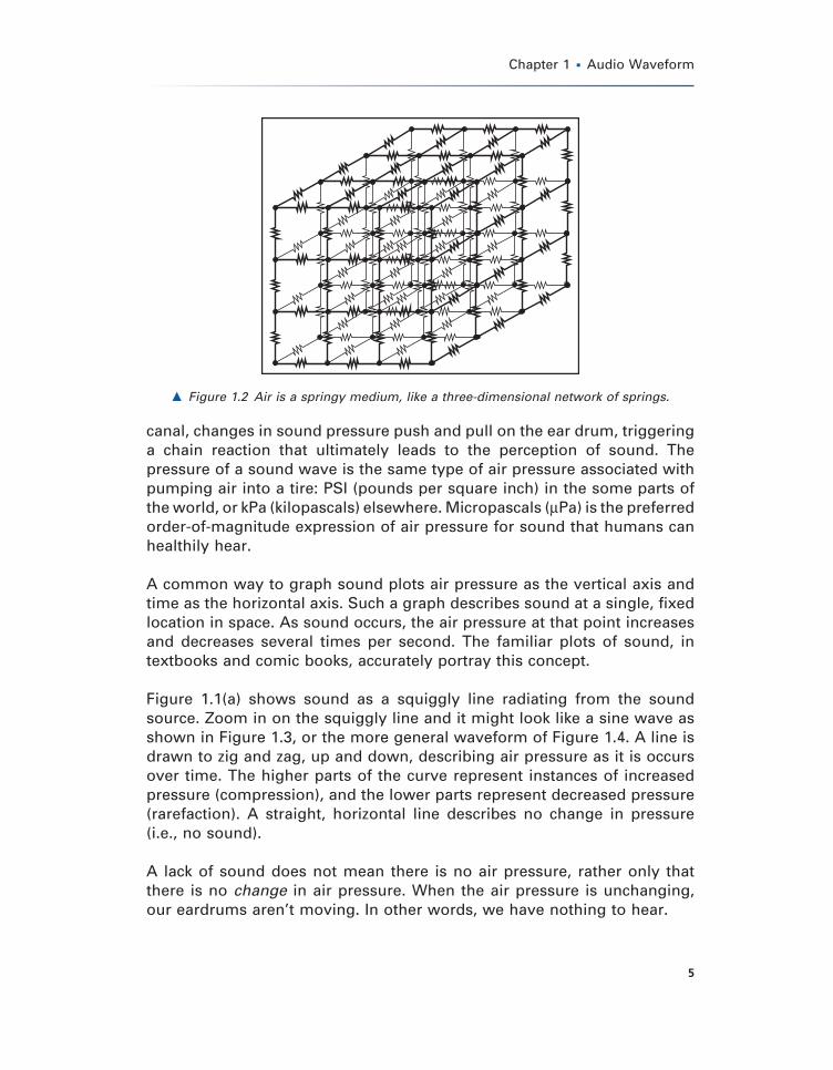
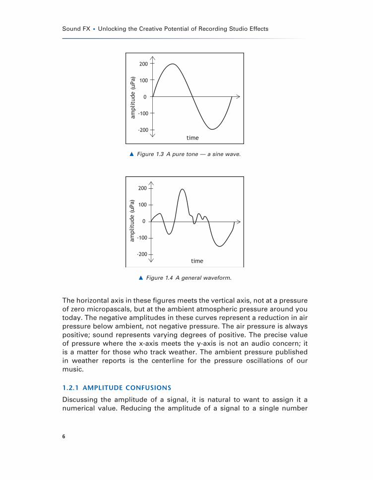
Figure 1.1(a) shows sound as a squiggly line radiating from the sound source. Zoom in on the squiggly line and it might look like a sine wave as shown in Figure 1.3, or the more general waveform of Figure 1.4. A line is drawn to zig and zag, up and down, describing air pressure as it is occurs over time. The higher parts of the curve represent instances of increased pressure (compression), and the lower parts represent decreased pressure (rarefaction). A straight, horizontal line describes no change in pressure (i.e., no sound).

A lack of sound does not mean there is no air pressure, rather only that there is no change in air pressure. When the air pressure is unchanging, our eardrums aren’t moving. In other words, we have nothing to hear.

� Figure 1.2 Air is a springy medium, like a three-dimensional network of springs.



6

The horizontal axis in these fi gures meets the vertical axis, not at a pressure of zero micropascals, but at the ambient atmospheric pressure around you today. The negative amplitudes in these curves represent a reduction in air pressure below ambient, not negative pressure. The air pressure is always positive; sound represents varying degrees of positive. The precise value of pressure where the x-axis meets the y-axis is not an audio concern; it is a matter for those who track weather. The ambient pressure published in weather reports is the centerline for the pressure oscillations of our music.

1.2.1 AMPLITUDE CONFUSIONS

Discussing the amplitude of a signal, it is natural to want to assign it a numerical value. Reducing the amplitude of a signal to a single number

� Figure 1.3 A pure tone — a sine wave.

� Figure 1.4 A general waveform.



7

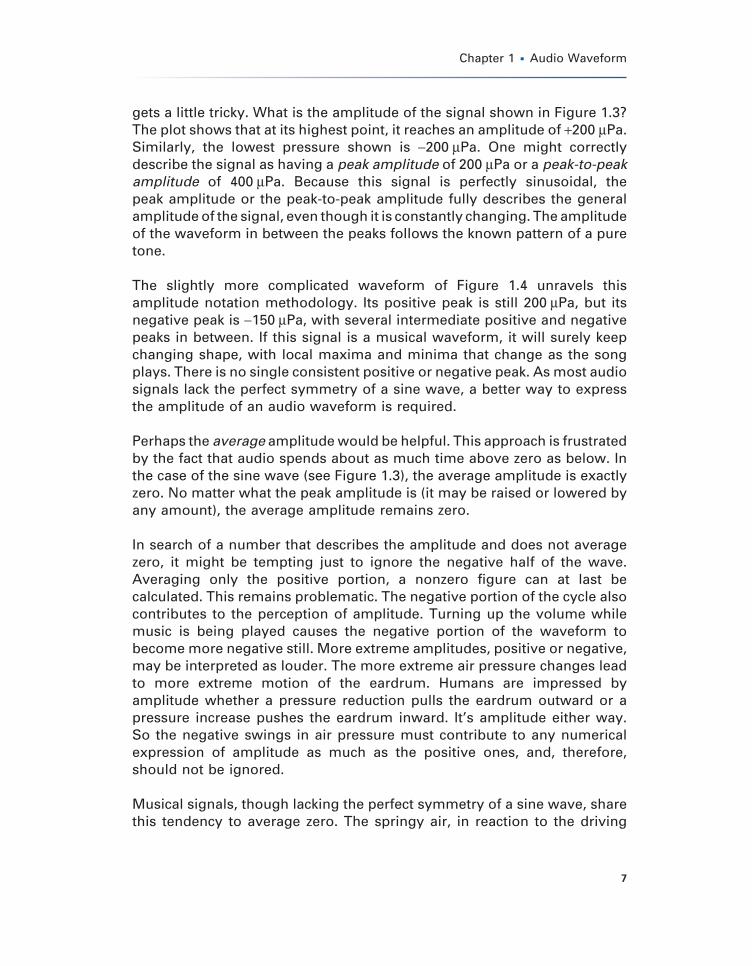
gets a little tricky. What is the amplitude of the signal shown in Figure 1.3? The plot shows that at its highest point, it reaches an amplitude of +200 µPa. Similarly, the lowest pressure shown is −200 µPa. One might correctly describe the signal as having a peak amplitude of 200 µPa or a peak-to-peak amplitude of 400 µPa. Because this signal is perfectly sinusoidal, the peak amplitude or the peak-to-peak amplitude fully describes the general amplitude of the signal, even though it is constantly changing. The amplitude of the waveform in between the peaks follows the known pattern of a pure tone.

The slightly more complicated waveform of Figure 1.4 unravels this amplitude notation methodology. Its positive peak is still 200 µPa, but its negative peak is −150 µPa, with several intermediate positive and negative peaks in between. If this signal is a musical waveform, it will surely keep changing shape, with local maxima and minima that change as the song plays. There is no single consistent positive or negative peak. As most audio signals lack the perfect symmetry of a sine wave, a better way to express the amplitude of an audio waveform is required.

Perhaps the average amplitude would be helpful. This approach is frustrated by the fact that audio spends about as much time above zero as below. In the case of the sine wave (see Figure 1.3), the average amplitude is exactly zero. No matter what the peak amplitude is (it may be raised or lowered by any amount), the average amplitude remains zero.

In search of a number that describes the amplitude and does not average zero, it might be tempting just to ignore the negative half of the wave. Averaging only the positive portion, a nonzero fi gure can at last be calculated. This remains problematic. The negative portion of the cycle also contributes to the perception of amplitude. Turning up the volume while music is being played causes the negative portion of the waveform to become more negative still. More extreme amplitudes, positive or negative, may be interpreted as louder. The more extreme air pressure changes lead to more extreme motion of the eardrum. Humans are impressed by amplitude whether a pressure reduction pulls the eardrum outward or a pressure increase pushes the eardrum inward. It’s amplitude either way. So the negative swings in air pressure must contribute to any numerical expression of amplitude as much as the positive ones, and, therefore, should not be ignored.

Musical signals, though lacking the perfect symmetry of a sine wave, share this tendency to average zero. The springy air, in reaction to the driving



8

action of a loudspeaker, compresses and stretches. Each pressure increase is followed by a pressure decrease. At the end of the song, the air returns to ambient pressure, the loudspeaker cone returns to its original position, and the eardrum returns to its starting point.

One way to allow the negative portion of the oscillating wave to contribute to the amplitude calculation is to average the absolute value of the amplitude. Make all negative amplitudes positive, keep all positive values positive, and fi nd the running average. The resulting expression for amplitude can track the perception of amplitude reasonably well. VU meters do exactly this, averaging the absolute value of the amplitude observed over the preceding 300 milliseconds.

There is further room for improvement: root mean square (RMS). Measuring RMS amplitude properly allows both negative and positive parts of the wave to infl uence the resulting number for amplitude. RMS might best be understood by working through the acronym in reverse. Square the amplitudes to be measured, so that a positive value always results. Take the mean (a.k.a. average) value of the amplitudes observed. Finally take the square root of the result to undo the fact that the contributing amplitudes were all squared before being averaged.

RMS amplitude is more convenient for scientists and equipment designers, as it is this type of average amplitude that must be used in calculations of energy, power, heat, etc. Audio engineering rarely needs such precision. The simpler absolute value average of the VU meter is almost always a suffi cient indicator of amplitude.

1.2.2 TIME IMPLICATIONS

The amplitude versus time plot reveals fundamental information about audio waveforms. A pure-tone sine wave (see Figure 1.3) consists of a simple, never-changing pattern of oscillation. Measure the length of time associated with each cycle to determine the waveform’s period. Count the number of times it cycles each second for a determination of its frequency. Period is the time it takes for exactly one cycle to occur, with units of seconds per dimensionless cycle, or simply seconds. Frequency describes the number of cycles that occur in exactly one second, with units of dimensionless cycles per second. Therefore, units for frequency live entirely in the denominator (per second, or /s) and have been given the alternative unit of hertz (Hz).



9

Note that counting the number of cycles per second (frequency) is the opposite of counting the number of seconds per cycle (period). Mathematically, they are reciprocals:

fT

= 1 (1.1)

and

Tf

= 1 (1.2)

where f = frequency, and T = period.

1.3 Amplitude versus DistanceThe springiness of air ensures that any localized changes in air pressure near a sound source will cause a chain reaction of air pressure changes, above and below the current air pressure, all around that source. Even a slight disturbance of air pressure will ripple outward. In order to describe the state of air pressure along some distance, a different pair of axes is needed: air pressure versus location or air pressure versus distance.

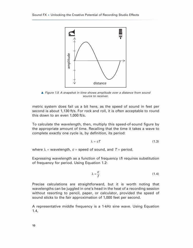
At a fi xed instant in time, a plot is made of the air pressure as a function of its location in space. Figure 1.5 shows such a snapshot. Returning to Figure 1.1(a), where an illustrator strategically failed to label any axes, one can conclude that the curves radiating outward from the sound source might be amplitude versus time or amplitude versus distance. The rings of Figure 1.1(b) present sound in a slightly different way. This familiar sketch of sound is a snapshot of amplitude versus distance, showing just the positive peaks of a propagating wave, or just the negative excursions, or just the zero crossings. Called isobars, the rings of sound radiating outward from the sound source indicate the spatial distribution of points of equi-valent pressure. This is a helpful image for audio engineers; it works in comics too.

The amplitude versus distance expression of sound leads to another fundamental property of waveforms: wavelength, which is the distance traveled during exactly one cycle. Drive 55 miles per hour for one hour, and the distance covered is exactly 55 miles. Distance traveled can be calculated through the multiplication of speed by time. The speed of sound in air (under normal temperature and pressure) is 344 m/s. The always-friendly



10

metric system does fail us a bit here, as the speed of sound in feet per second is about 1,130 ft/s. For rock and roll, it is often acceptable to round this down to an even 1,000 ft/s.

To calculate the wavelength, then, multiply this speed-of-sound fi gure by the appropriate amount of time. Recalling that the time it takes a wave to complete exactly one cycle is, by defi nition, its period:

λ = cT (1.3)

where λ = wavelength, c = speed of sound, and T = period.

Expressing wavelength as a function of frequency (f) requires substitution of frequency for period. Using Equation 1.2:

λ = cf

(1.4)

Precise calculations are straightforward, but it is worth noting that wavelengths can be juggled in one’s head in the heat of a recording session without resorting to pencil, paper, or calculator, provided the speed of sound sticks to the fair approximation of 1,000 feet per second.

A representative middle frequency is a 1-kHz sine wave. Using Equation 1.4,

� Figure 1.5 A snapshot in time shows amplitude over a distance from sound source to receiver.



11

λ

λ

=

=

cf

1 0001 0001 000

,,,

ft sHz

(1.5)

Recalling the units underlying hertz are cycles per second (/s),

λ1 000

1 0001 000

,,,

= ft ss

(1.6)

which leads to the fi nal result for the convenient, approximate wavelength for a 1,000-Hz sine wave:

λ1,000 = 1 ft (1.7)

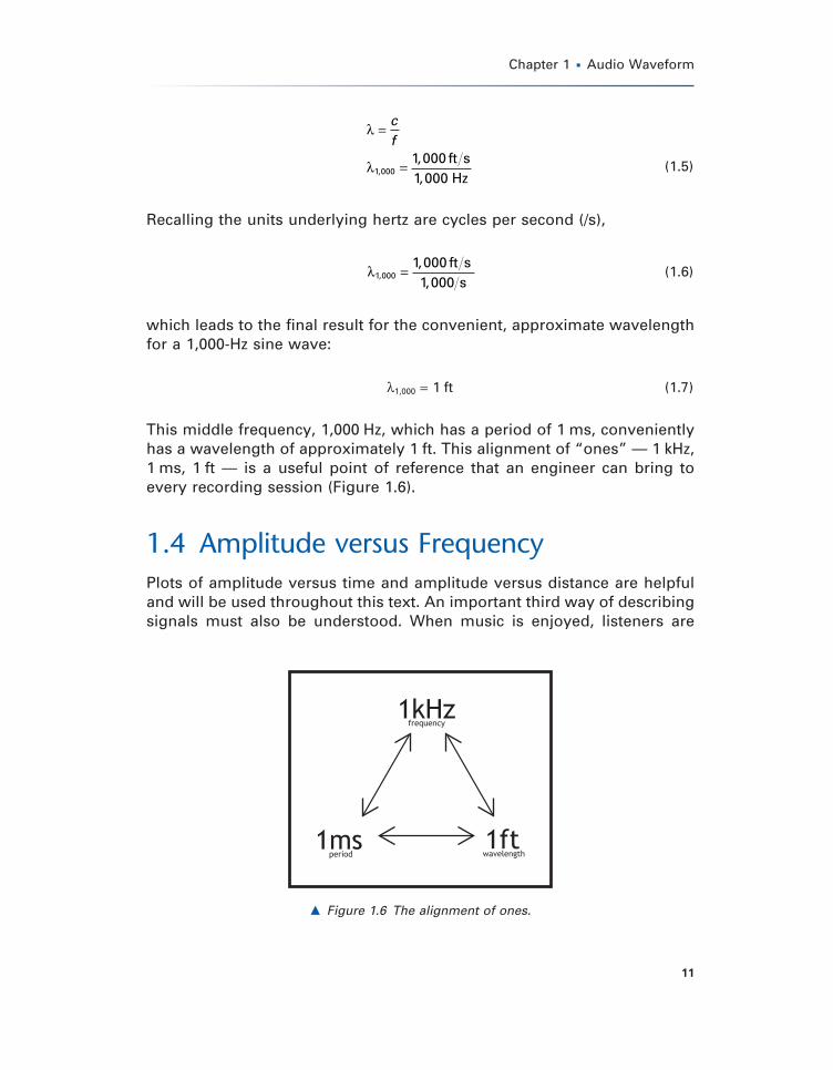
This middle frequency, 1,000 Hz, which has a period of 1 ms, conveniently has a wavelength of approximately 1 ft. This alignment of “ones” — 1 kHz, 1 ms, 1 ft — is a useful point of reference that an engineer can bring to every recording session (Figure 1.6).

1.4 Amplitude versus FrequencyPlots of amplitude versus time and amplitude versus distance are helpful and will be used throughout this text. An important third way of describing signals must also be understood. When music is enjoyed, listeners are

� Figure 1.6 The alignment of ones.



12

certainly aware that there are changes in amplitude over time at whatever location they currently occupy. Without a computer screen in front of them offering the information visually, listeners don’t consciously pay attention to the fi ne details shown in the amplitude versus time plots.

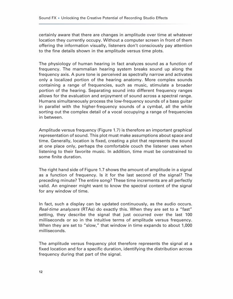
The physiology of human hearing in fact analyzes sound as a function of frequency. The mammalian hearing system breaks sound up along the frequency axis. A pure tone is perceived as spectrally narrow and activates only a localized portion of the hearing anatomy. More complex sounds containing a range of frequencies, such as music, stimulate a broader portion of the hearing. Separating sound into different frequency ranges allows for the evaluation and enjoyment of sound across a spectral range. Humans simultaneously process the low-frequency sounds of a bass guitar in parallel with the higher-frequency sounds of a cymbal, all the while sorting out the complex detail of a vocal occupying a range of frequencies in between.

Amplitude versus frequency (Figure 1.7) is therefore an important graphical representation of sound. This plot must make assumptions about space and time. Generally, location is fi xed, creating a plot that represents the sound at one place only, perhaps the comfortable couch the listener uses when listening to their favorite music. In addition, time must be constrained to some fi nite duration.

The right hand side of Figure 1.7 shows the amount of amplitude in a signal as a function of frequency. Is it for the last second of the signal? The preceding minute? The entire song? These time increments are all perfectly valid. An engineer might want to know the spectral content of the signal for any window of time.

In fact, such a display can be updated continuously, as the audio occurs. Real-time analyzers (RTAs) do exactly this. When they are set to a “fast” setting, they describe the signal that just occurred over the last 100 milliseconds or so in the intuitive terms of amplitude versus frequency. When they are set to “slow,” that window in time expands to about 1,000 milliseconds.

The amplitude versus frequency plot therefore represents the signal at a fi xed location and for a specifi c duration, identifying the distribution across frequency during that part of the signal.



13

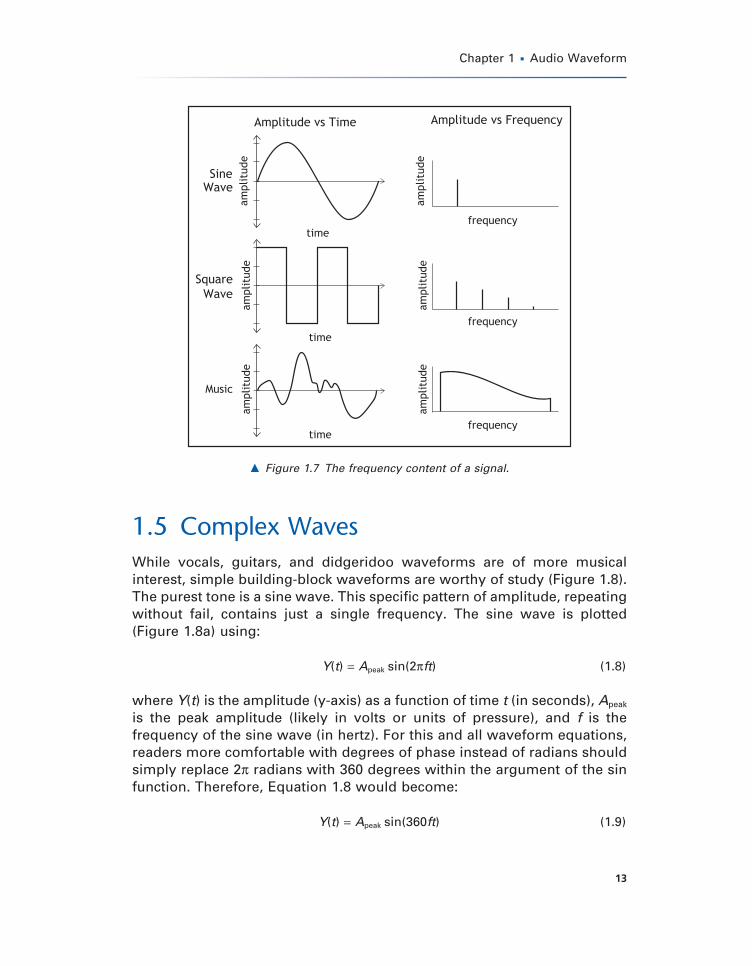
1.5 Complex WavesWhile vocals, guitars, and didgeridoo waveforms are of more musical interest, simple building-block waveforms are worthy of study (Figure 1.8). The purest tone is a sine wave. This specifi c pattern of amplitude, repeating without fail, contains just a single frequency. The sine wave is plotted (Figure 1.8a) using:

Y(t) = Apeak sin(2πft) (1.8)

where Y(t) is the amplitude (y-axis) as a function of time t (in seconds), Apeak is the peak amplitude (likely in volts or units of pressure), and f is the frequency of the sine wave (in hertz). For this and all waveform equations, readers more comfortable with degrees of phase instead of radians should simply replace 2π radians with 360 degrees within the argument of the sin function. Therefore, Equation 1.8 would become:

Y(t) = Apeak sin(360ft) (1.9)

� Figure 1.7 The frequency content of a signal.



14

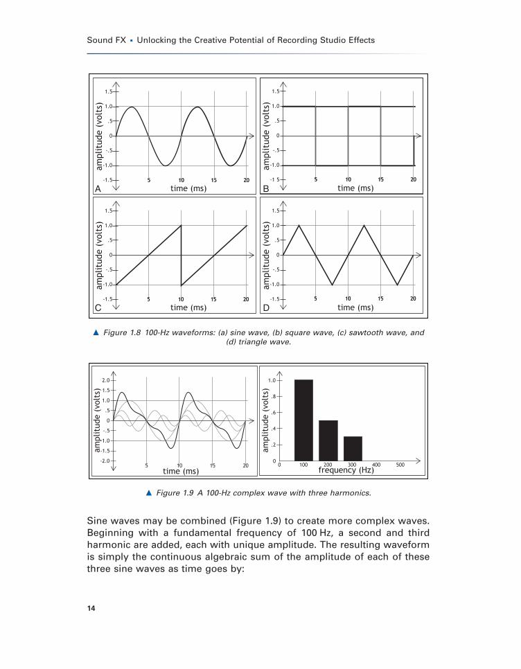
Sine waves may be combined (Figure 1.9) to create more complex waves. Beginning with a fundamental frequency of 100 Hz, a second and third harmonic are added, each with unique amplitude. The resulting waveform is simply the continuous algebraic sum of the amplitude of each of these three sine waves as time goes by:

� Figure 1.8 100-Hz waveforms: (a) sine wave, (b) square wave, (c) sawtooth wave, and (d) triangle wave.

� Figure 1.9 A 100-Hz complex wave with three harmonics.

A B

C D



15

Y(t) = A1 sin(2πft) + A2 sin(2π2ft) + A3 sin(2π3ft) (1.10)

where An is the amplitude of the nth harmonic. In Figure 1.9,

Y(t) = sin(2πft) + 0.5 sin(2π2ft) + 0.25 sin(2π3ft) (1.11)

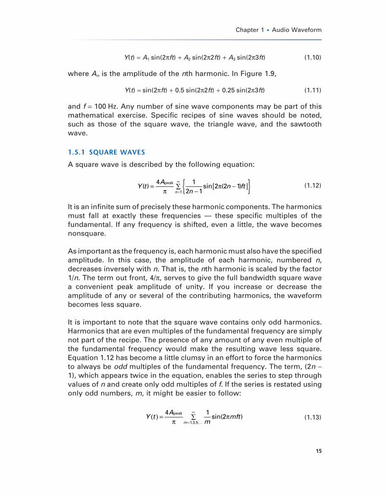
and f = 100 Hz. Any number of sine wave components may be part of this mathematical exercise. Specifi c recipes of sine waves should be noted, such as those of the square wave, the triangle wave, and the sawtooth wave.

1.5.1 SQUARE WAVES

A square wave is described by the following equation:

Y tA

nn ft

n( ) ( )=

−−[ ]{ }∑

=

∞4 12 1

2 2 11

peaksin

ππ (1.12)

It is an infi nite sum of precisely these harmonic components. The harmonics must fall at exactly these frequencies — these specifi c multiples of the fundamental. If any frequency is shifted, even a little, the wave becomes nonsquare.

As important as the frequency is, each harmonic must also have the specifi ed amplitude. In this case, the amplitude of each harmonic, numbered n, decreases inversely with n. That is, the nth harmonic is scaled by the factor 1/n. The term out front, 4/π, serves to give the full bandwidth square wave a convenient peak amplitude of unity. If you increase or decrease the amplitude of any or several of the contributing harmonics, the waveform becomes less square.

It is important to note that the square wave contains only odd harmonics. Harmonics that are even multiples of the fundamental frequency are simply not part of the recipe. The presence of any amount of any even multiple of the fundamental frequency would make the resulting wave less square. Equation 1.12 has become a little clumsy in an effort to force the harmonics to always be odd multiples of the fundamental frequency. The term, (2n − 1), which appears twice in the equation, enables the series to step through values of n and create only odd multiples of f. If the series is restated using only odd numbers, m, it might be easier to follow:

Y t

Am

mftm

( ), , , . .

= ∑=

∞4 12

1 3 5

peaksin( )

ππ (1.13)



16

� Figure 1.10 100-Hz square wave through the addition of harmonics up to (a) 500 Hz (3 harmonics), (b) 1,000 Hz (5 harmonics), (c) 2,500 Hz (13 harmonics), and 5,000 Hz

(25 harmonics).



17

A square wave with a fundamental frequency of 100 Hz and a peak amplitude of 1 volt (Figure 1.8b) uses Equation 1.12 or 1.13 to create:

Y t t t t1004

2 10013

15

2 50017

( ) = + +

+π

π π πsin( ) sin(2 300 ) sin( ) sin(( )2 700π t +

. . . (1.14)

The signifi cance of the harmonics is shown in Figure 1.10. The contribution of evermore upper harmonics, in strict adherence to the amplitudes and frequencies specifi ed, is clear through visual inspection. The waveform becomes increasingly more square as the bandwidth reaches upward and the number of harmonics included in the summation grows.

This makes clear the need for wide-bandwidth audio systems when square waves (think MIDI, SMPTE, and digital audio) are to be recorded and transmitted. A cable that rolls off the high frequencies of the signal within will attenuate the necessary harmonics that make up a square wave, in effect making a square wave less square. A perfectly square wave is achieved only through the rather impractical inclusion of an infi nite number of the prescribed harmonics.

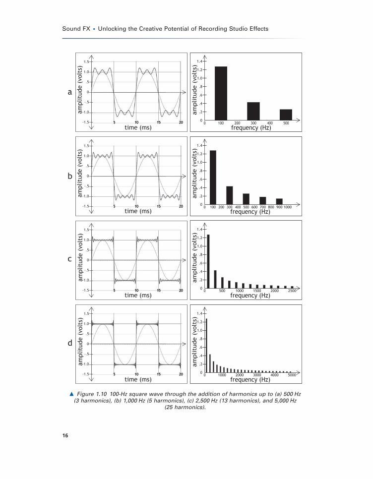
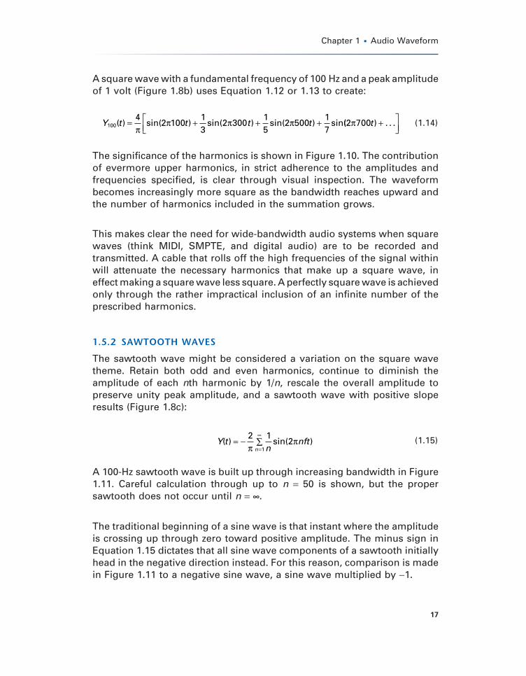
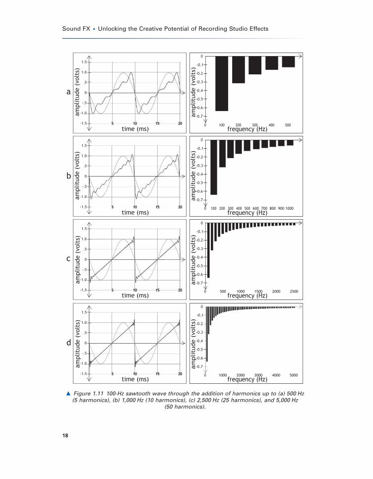
1.5.2 SAWTOOTH WAVES

The sawtooth wave might be considered a variation on the square wave theme. Retain both odd and even harmonics, continue to diminish the amplitude of each nth harmonic by 1/n, rescale the overall amplitude to preserve unity peak amplitude, and a sawtooth wave with positive slope results (Figure 1.8c):

Y tn

nftn

( ) = − ∑=

∞2 11π

πsin(2 ) (1.15)

A 100-Hz sawtooth wave is built up through increasing bandwidth in Figure 1.11. Careful calculation through up to n = 50 is shown, but the proper sawtooth does not occur until n = •.

The traditional beginning of a sine wave is that instant where the amplitude is crossing up through zero toward positive amplitude. The minus sign in Equation 1.15 dictates that all sine wave components of a sawtooth initially head in the negative direction instead. For this reason, comparison is made in Figure 1.11 to a negative sine wave, a sine wave multiplied by −1.



18

� Figure 1.11 100-Hz sawtooth wave through the addition of harmonics up to (a) 500 Hz (5 harmonics), (b) 1,000 Hz (10 harmonics), (c) 2,500 Hz (25 harmonics), and 5,000 Hz

(50 harmonics).



19

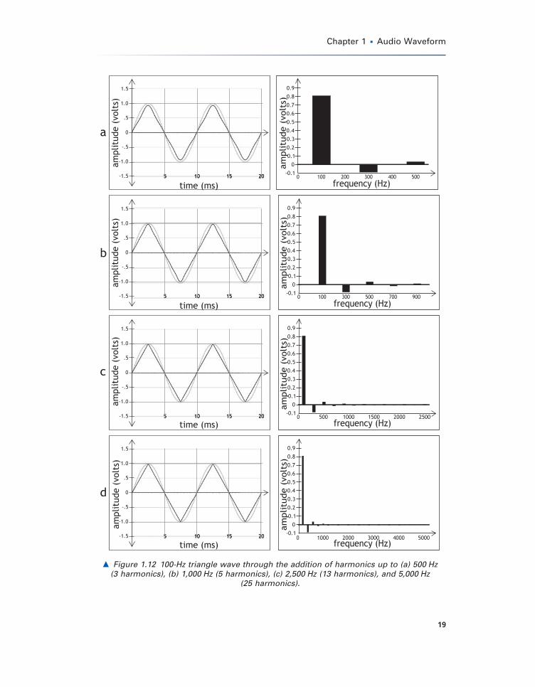
� Figure 1.12 100-Hz triangle wave through the addition of harmonics up to (a) 500 Hz (3 harmonics), (b) 1,000 Hz (5 harmonics), (c) 2,500 Hz (13 harmonics), and 5,000 Hz

(25 harmonics).



20

The sum of all sine waves in the equation (an infi nite number of precisely scaled multiples of fundamental frequency f ) causes the net wave to leap to −1 before steadily rising toward +1. The instant when the saw-tooth wave reaches +1 is also the fortuitous instant when each and every component harmonic happens to be beginning a negative cycle anew. This symphony of sine waves crossing upward through zero but multiplied by −1 causes the net amplitude to snap to −1 again. The pattern repeats.

1.5.3 TRIANGLE WAVES

The triangle wave (Figure 1.8d) comes from a different set of carefully scaled odd harmonics:

Y tA

nn ft

n

n( )

( )( )

( )

= −−

−[ ]∑−

=

∞8 12 1

2 2 12

1

21

peak

ππ (1.16)

In addition to the requisite scaling to achieve unity peak amplitude and the use of the term (2n − 1) to generate odd harmonics, notice the additional need for an alternating polarity among the harmonic components. The term, −1(n−1) causes the harmonics to switch sign with each increment of n. The polarity of every other harmonic is positive, while the polarity of each harmonic in between is negative. The summation of these particular components, some adding to the total while others subtract, leads to a triangle wave.

Figure 1.12 demonstrates the signifi cance of adding additional harmonics to the fundamental sine wave. As the amplitude of successive harmonics falls proportional to 1/n2, this complex wave is more dependent on lower harmonics than the square and sawtooth waves. This is evident in two ways. Note the towering signifi cance of the lower harmonics on the right-hand side of Figure 1.12. Note also how the wave obtains its characteristic sharpness and comes quite close to resembling the full bandwidth shape with just 13 harmonics.

Very much as multitrack music is built from a mix of component production elements such as drums, bass, keys, and vocals, individual pitched waveforms that make up each multitrack element are themselves made up of a specifi c mix of sinusoidal components. It is our job to make art from these humble ingredients.



21

1.6 DecibelIt is diffi cult to do anything in audio and not encounter the decibel. As discussed below, the decibel offers a precise calculation that quantifi es properties of an audio signal in a very useful form. The fact is one may never trouble to dig out these equations and perform a decibel calculation during the course of a recording session. But the hardware designers and software code jockeys who create the effects processors and recording devices that fi ll the studio certainly do. If an audio engineer is to speak comfortably and accurately about decibels, it helps to know a little of the math that makes it possible. Those who are bored or frustrated by the math should at least know that someone went to a lot of trouble to fi nd a way to express the level of the signal in a way analogous to the expression of pitch. The decibel offers a perceptually meaningful description of amplitude, one that the ears and brain can make sense of.

The decibel appears in some form on almost every faceplate and every user interface of every signal processor in the recording studio. Understanding the meaning of quantities in decibels is essential to understanding sound effects. There is an equation that absolutely defi nes the decibel (dB):

dB logpowerpower

10A

B

= ×

10 (1.17)

The English translation of that equation goes something like, “The decibel is ten times the logarithm of the ratio of two powers.” This straightforward statement is rich with meaning.

The equation for the decibel has two features built-in. First is the logarithm. The mathematical properties of this function are considered in detail shortly, but it is important to understand the motivation for digging up the logarithmic, or log, function in the fi rst place. The log is part of the decibel equation to make the math more convenient. It makes the vast range of amplitudes typical of audio much easier to deal with.

The second key element of the decibel equation is the ratio of powers within parentheses. The decibel equation uses a ratio so as to be consistent with the human perception of power and related quantities. The equation attempts to create a number that describes the amplitude of a musical waveform. For the decibel to be useful, the resulting number needs



22

to have some connection to the human perception of this property of sound.

These two feature — log and ratio — make the decibel a versatile and useful way to express the amplitude of our musical waveforms.

1.6.1 LOGARITHM

The log represents nothing more than a reshuffl ing of how the numbers are expressed. The two following equations are both true and say very nearly the same thing:

10y = X (1.18)

log10X = y (1.19)

Equation 1.18 is relatively straightforward. Ten raised to the power y gives the result X. For example:

103 = 10 ¥ 10 ¥ 10 = 1,000 (1.20)

The logarithm enables us to undo the calculation mathematically. Starting with the answer from above, 1,000, the log function leads back to 3.

log10(1,000) = 3 (1.21)

Said another way, Equation 1.19 answers the question, “What power of 10 will give us this number, X?” To take the log of 1,000 as in Equation 1.21 is to ask, “What power of 10 gives us 1,000?” The answer is 3: 103 = 1,000, so log10(1,000) = 3.

What power of 10 will give us 1,000,000? With an eye for powers of 10, or perhaps with the help of a calculator, it is easily confi rmed that the log10(1,000,000) = 6. Ten raised to the sixth power gives us one million, as Equation 1.9 would describe it. Now calculate the power of 10 that gives 100 trillion: log10(100,000,000,000,000) = 14.

Herein lies the motivation for logarithms in audio. They make big numbers — potentially very big numbers — much smaller: 100,000,000,000,000 becomes 14. It converts governmental budgets into football scores.

The log function is an acquired taste. Those with little or no exposure to them will likely fi nd the logarithm awkward at fi rst.



23

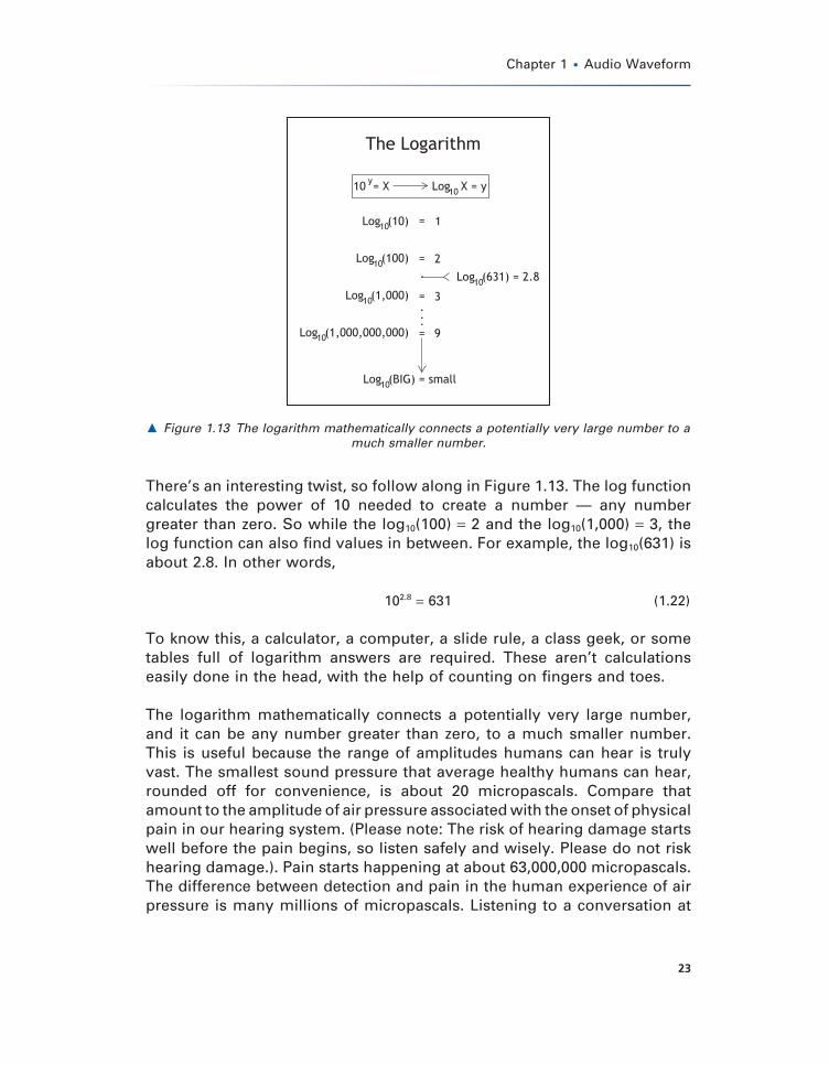
There’s an interesting twist, so follow along in Figure 1.13. The log function calculates the power of 10 needed to create a number — any number greater than zero. So while the log10(100) = 2 and the log10(1,000) = 3, the log function can also fi nd values in between. For example, the log10(631) is about 2.8. In other words,

102.8 = 631 (1.22)

To know this, a calculator, a computer, a slide rule, a class geek, or some tables full of logarithm answers are required. These aren’t calculations easily done in the head, with the help of counting on fi ngers and toes.

The logarithm mathematically connects a potentially very large number, and it can be any number greater than zero, to a much smaller number. This is useful because the range of amplitudes humans can hear is truly vast. The smallest sound pressure that average healthy humans can hear, rounded off for convenience, is about 20 micropascals. Compare that amount to the amplitude of air pressure associated with the onset of physical pain in our hearing system. (Please note: The risk of hearing damage starts well before the pain begins, so listen safely and wisely. Please do not risk hearing damage.). Pain starts happening at about 63,000,000 micropascals. The difference between detection and pain in the human experience of air pressure is many millions of micropascals. Listening to a conversation at

� Figure 1.13 The logarithm mathematically connects a potentially very large number to a much smaller number.



24

normal levels might occur with amplitudes of around 20,000 micropascals. It is reasonable to monitor a pop mix at about 630,000 micropascals. One might occasionally crank it to more than 6,000,000 micropascals. Even at this level, the neighbors aren’t complaining, the drummer wants it louder, and, if it doesn’t go on for too long, there isn’t much risk of hearing damage yet. Jet engines and power plants are much, much louder still, on the order of hundreds of millions of micropascals.

The problem with these numbers is clear: they are too big to be useful in the studio. “Yeah, let me push the snare up about 84, pull the strings down about 6,117, and see if the mix sits right at 1,792,000.” This is too awkward; the decibel to the rescue. The mathematical log function exhibits the following helpful property:

log10(BIG) = small (1.23)

The log of a big number results in a much smaller number. Human hearing is capable of interpreting a vast range of amplitudes. The numbers used to describe amplitude become unwieldy if not routinely subjected to the logarithm, so it is a fundamental part of the decibel equation.

1.6.2 RATIOS

Also built into the decibel equation is a ratio (consult again Equation 1.17). Mathematically, a ratio strategically reduces two numbers to a single, informative number.

Consider pitch. Musical harmony is built on ratios. The octave, for example, represents a doubling of pitch, a ratio of 2 : 1. The orchestra tunes (generally) to A440. Also identifi ed as A4, this is the fi rst A above middle C. A440 is a musical note whose fundamental frequency is exactly 440 Hz. Double that frequency to 880 Hz to create a note exactly one octave higher. To lower the pitch by exactly one octave, reverse the ratio (e.g., 1 : 2, or mathematically, 1/2 = 0.5). That is, cut the frequency in half. An octave below A440 has a fundamental frequency of 220 Hz.

All the musical intervals represent ratios. The numerical value of the ratio represents a scaling factor that, when multiplied by the starting frequency, fi nds the new frequency needed to reach the desired musical interval. As the intervals deviate from the octave, the ratios are no longer built on simple whole numbers, and the exact ratios depend on the type of tuning used. For example, a perfect fi fth is a ratio of 3 : 2 (3/2 = 1.5) in just intonation.



25

In equal-tempered tuning, a perfect fi fth is achieved by multiplying by about 1.498. A perfect fourth represents the ratio of 4 : 3 (4/3 = 1.3333) in just intonation, but the slightly different 1.3348 for equal temperament. No matter which form of tuning is selected, it is always a ratio that rules. In order to create a note that is a specifi ed musical interval away, multiply the starting pitch by the value of the appropriate ratio.

It doesn’t make musical sense to think in terms of the actual number of hertz between two notes. A big band arranger won’t ask the trumpet player to play 217 Hz above the tenor sax. Instead, ratios are used. Score the horn a minor third above, or an octave above, and the trumpeter can oblige.

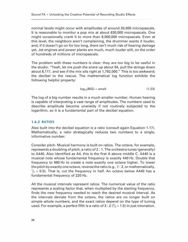
Looking at Figure 1.14, consider each note’s fundamental pitches mathe-matically, not musically. Start two E’s below middle C, labeled E2. It has a fundamental frequency of about 821/2 Hz — a meaningless observation for the performing musician, perhaps, but an important one for the recording musician. Up one octave, the pitch is exactly twice the starting pitch. That’s the very defi nition of an octave. One octave up leads to E3, with a fundamental pitch of about 165 Hz (2 ¥ 82.5). One more octave up is E4, the fi rst E above middle C. E4 has a fundamental pitch of about 330 Hz. E5 is yet another octave above and has a pitch of about 660 Hz. Four pitches, one musical value. They are all labeled “E,” and they all sound very similar, musically speaking. In harmony, E at any octave performs very nearly identical functions.

What’s the difference between one E natural and the next E up? An octave. But there’s a subtle illusion going on here. Using Figure 1.14, watch as the absolute numbers fail and the ratio takes over. The “distance” (as measured in hertz) from E2 to E3 is 82 Hz. This 82-Hz difference has meaning to the human hearing system; it’s an octave. Starting at E3 and going up to E4 traverses an octave again. However, measured in hertz, this octave represents a difference of 165 Hz. E4 to E5 is an octave, worth 330 Hz.

� Figure 1.14 Frequency changes of the octave.



26

An octave equals 82 Hz in one instance, 165 Hz in another situation, and then 330 Hz in the third case. The octave cannot be expressed in hertz unless the starting pitch is known. It can always be expressed as a ratio: 2 : 1.

The musical signifi cance of the octave is well known, offering the most consonant (i.e., least dissonant) pairing of two notes of different pitches. Experienced musicians also attach specifi c sensory meaning to many (probably all) of the other intervals: the buzz of the perfect fi fth, the warmth of the major third, and the bittersweet mood of the minor seventh. Such complex, advanced human feelings about the pitch differences between two notes reduce almost insultingly to some pretty straightforward math. To go up an octave, multiply by 2. Done. It doesn’t matter what the starting pitch is.

Minor headache: Beyond the octave, the numbers aren’t so neat. To go up a perfect fi fth in the most common form of tuning in pop music, equal temperament, simply multiply by about 1.49830708. To go up a major third (in equal-tempered tuning) multiply by the unwieldy (and rounded off) 1.25992105. The numbers are rather unappealing. But the fundamental principle is comfortingly straightforward. Don’t add a certain number of hertz to go up by a certain musical amount. Instead, multiply by the numerical value of the appropriate ratio.

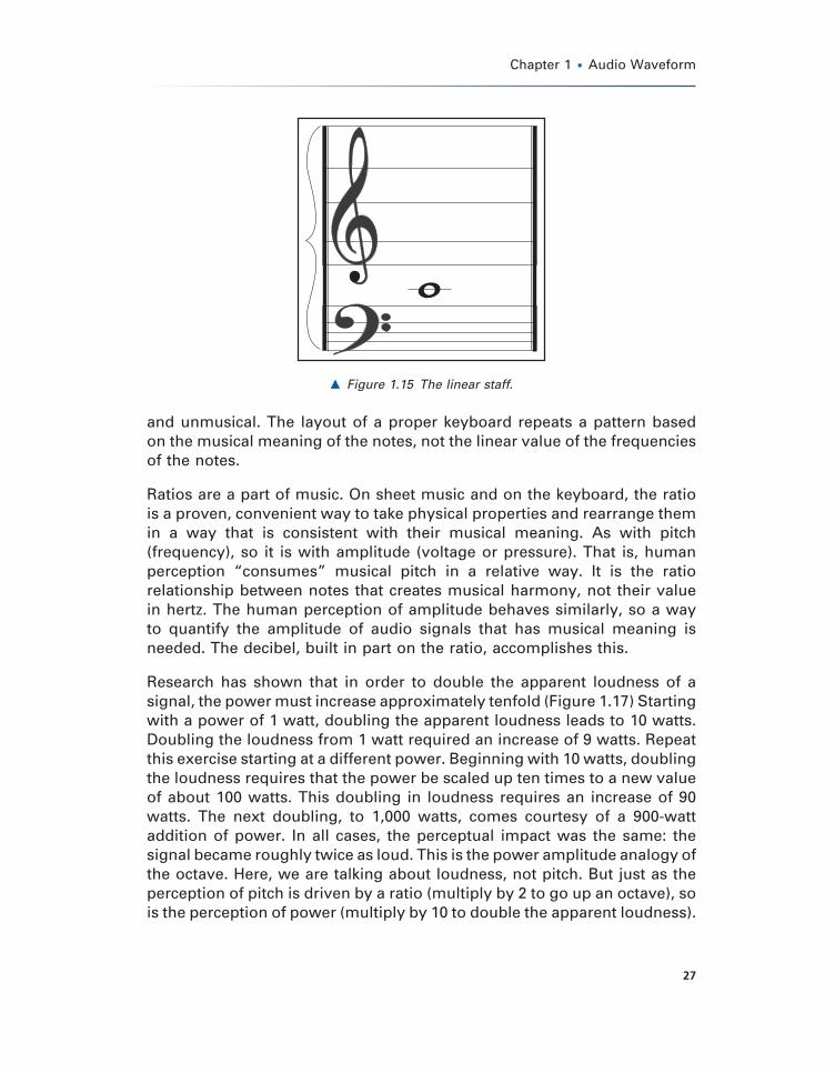
The idea of the ratio is built into our musical pitch-labeling scheme. Notes are described on the familiar musical staff and labeled with the familiar short, repeating alphabet from A to G. Peek at the numbers and something peculiar is revealed. If we plot the musical staff using linear mathematics, in which all the lines and spaces of our traditional notation system are spaced an equal number of hertz apart rather than simply an equal distance apart, we get the rather strange looking staff shown in Figure 1.15. The traditional notation scheme masks the actual quantities involved — for good reason. The musical relevance of the notes is captured in the notation system. The relationship between C and G is always the same: it’s a perfect fi fth at any octave at any location on the staff. Therefore, it is shown that way on paper. It isn’t musically important how many hertz apart two notes are, but it is certainly important how many lines and spaces apart they are, as arrangers well know.

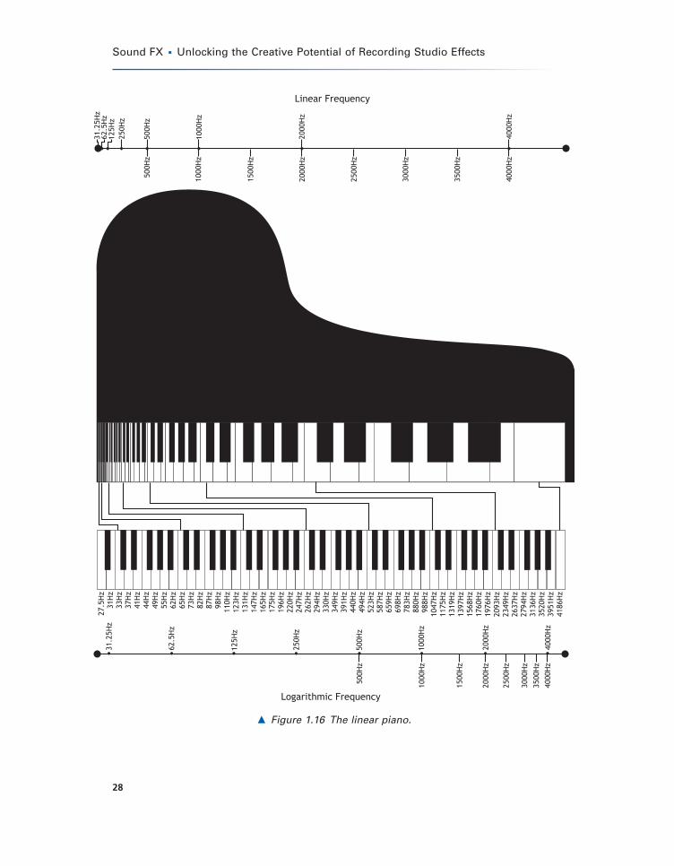
The keyboard of the piano presents the same illusion, physically. Figure 1.16 shows a piano in which the number of hertz between the notes determines the physical size and location of the keys, which are unplayable



27

and unmusical. The layout of a proper keyboard repeats a pattern based on the musical meaning of the notes, not the linear value of the frequencies of the notes.

Ratios are a part of music. On sheet music and on the keyboard, the ratio is a proven, convenient way to take physical properties and rearrange them in a way that is consistent with their musical meaning. As with pitch (frequency), so it is with amplitude (voltage or pressure). That is, human perception “consumes” musical pitch in a relative way. It is the ratio relationship between notes that creates musical harmony, not their value in hertz. The human perception of amplitude behaves similarly, so a way to quantify the amplitude of audio signals that has musical meaning is needed. The decibel, built in part on the ratio, accomplishes this.

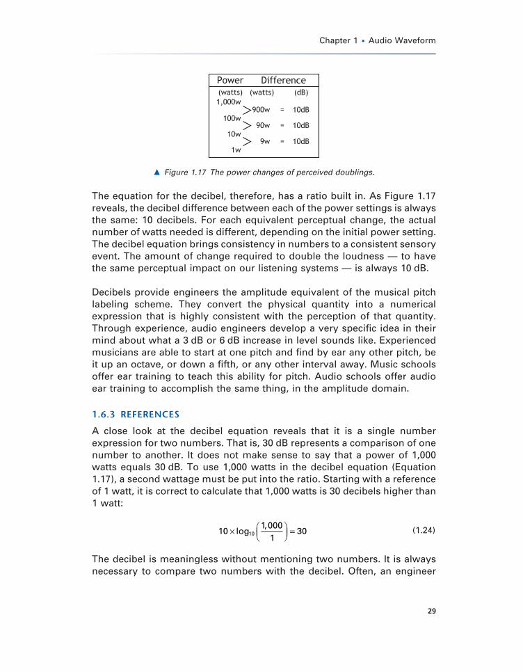
Research has shown that in order to double the apparent loudness of a signal, the power must increase approximately tenfold (Figure 1.17) Starting with a power of 1 watt, doubling the apparent loudness leads to 10 watts. Doubling the loudness from 1 watt required an increase of 9 watts. Repeat this exercise starting at a different power. Beginning with 10 watts, doubling the loudness requires that the power be scaled up ten times to a new value of about 100 watts. This doubling in loudness requires an increase of 90 watts. The next doubling, to 1,000 watts, comes courtesy of a 900-watt addition of power. In all cases, the perceptual impact was the same: the signal became roughly twice as loud. This is the power amplitude analogy of the octave. Here, we are talking about loudness, not pitch. But just as the perception of pitch is driven by a ratio (multiply by 2 to go up an octave), so is the perception of power (multiply by 10 to double the apparent loudness).

� Figure 1.15 The linear staff.



28

� Figure 1.16 The linear piano.



29

The equation for the decibel, therefore, has a ratio built in. As Figure 1.17 reveals, the decibel difference between each of the power settings is always the same: 10 decibels. For each equivalent perceptual change, the actual number of watts needed is different, depending on the initial power setting. The decibel equation brings consistency in numbers to a consistent sensory event. The amount of change required to double the loudness — to have the same perceptual impact on our listening systems — is always 10 dB.

Decibels provide engineers the amplitude equivalent of the musical pitch labeling scheme. They convert the physical quantity into a numerical expression that is highly consistent with the perception of that quantity. Through experience, audio engineers develop a very specifi c idea in their mind about what a 3 dB or 6 dB increase in level sounds like. Experienced musicians are able to start at one pitch and fi nd by ear any other pitch, be it up an octave, or down a fi fth, or any other interval away. Music schools offer ear training to teach this ability for pitch. Audio schools offer audio ear training to accomplish the same thing, in the amplitude domain.

1.6.3 REFERENCES

A close look at the decibel equation reveals that it is a single number expression for two numbers. That is, 30 dB represents a comparison of one number to another. It does not make sense to say that a power of 1,000 watts equals 30 dB. To use 1,000 watts in the decibel equation (Equation 1.17), a second wattage must be put into the ratio. Starting with a reference of 1 watt, it is correct to calculate that 1,000 watts is 30 decibels higher than 1 watt:

101 000

130×

=log10

, (1.24)

The decibel is meaningless without mentioning two numbers. It is always necessary to compare two numbers with the decibel. Often, an engineer

� Figure 1.17 The power changes of perceived doublings.



30

wishes to make statements that compare amplitude to the current value, as in, “Turn the snare up 3 dB.” That is shorthand for, “Make the amplitude of the snare 3 decibels louder than the current amplitude.” If one were to resort to the equation, the current amplitude is used in the bottom of the ratio (the denominator), and the top of the ratio (the numerator) gets the amplitude of the new, louder snare that is desired. Of course, this equation is never used during a session. The faders on a computer screen or on a mixer are labeled in decibels already. Someone else already did the calculations for us.

If a signal isn’t being compared to its current value, then it is compared to some reference value. A good starting point might be a reference of 1 watt; 10 watts is 10 dB above this reference, and 100 watts is 20 dB above the same reference. So the correct way to express decibels here is something like, “100 watts is 20 decibels above the reference of 1 watt.”

It gets tiring, always expressing a value in decibels above or below some reference value. Here’s the time saver: If the reference is 1 watt, express it as dBW (pronounced, “dee bee double you”). The “W” tacked on to the end identifi es the reference as exactly 1 watt. This shortens the statement to, “100 watts is 20 dBW.” Done. The reference, which is required for the decibel statement to be meaningful, is attached to the dB abbreviation.

Note that the statement is not, “100 watts is 20 dB.” That is incorrect. A single number is not expressible as a decibel. There must be some value stated as a point of comparison. Using “dBW” instead of just “dB” is the subtle addition that gives these statements meaning.

So while Equation 1.17 is the general equation for the decibel, a more specifi c equation using a reference of 1 watt is helpful:

dBW logpower1watt

10= ×

10 (1.25)

Other subequations exist, with different reference values. For example, sometimes 1 watt is too big to be a useful reference power. Use the much smaller milliwatt (0.001 watt) instead. If the power reference is one milliwatt, the suffi x attached to dB is a lower case “m,” for milli:

dBm logpower

watt10= ×

100 001.

(1.26)



31

A little physics lets us leave the power domain and create expressions based on the quantities we see more often in the studio: sound pressure and voltage. Sound pressure decibel expressions use the threshold of hearing (20 micropascals) as the reference pressure, and we tack on the suffi x “SPL” to express sound pressure level in terms that have perceptual meaning:

dBSPL logpressure

Pa10= ×

2020 µ

(1.27)

Note that the equation changes a little. Instead of multiplying the logarithm by 10, sound pressure statements require multiplication by 20. This is a result of the physical relationship between acoustic power and sound pressure. Power is proportional to pressure squared. The sound power terms within Equation 1.17 become sound pressure squared instead. It is a property of logarithms that this power of two within the logarithm may be converted to multiplication by two outside the logarithm. Hence the 10 becomes 20 for decibel calculations related to pressure. Likewise, we can use decibels to describe the voltage in our gear. Electrical power is proportional to voltage squared, so again we use a 20 instead of a 10 in the decibel calculations for voltage.

In the voltage domain, a few references must be dealt with:

dBu logvoltage

volt10= ×

200 775. (1.28)

dBV logvoltage

volt10= ×

201 (1.29)

It is a quirk of history that the unwieldy reference of 0.775 volt was chosen. The interested reader can use Ohm’s Law to apply a standard 1 milliwatt of power across a load of 600 ohms (which was a standard in the early telecommunications industry, not audio). A voltage of 0.775 V results. Even as the idea of a 600-ohm load lost its signifi cance in the modern professional audio industry, the quirky standard voltage remains. Someone, tired of the clumsiness of that number, chose an easier to remember reference: 1 volt. Good idea. Confusing result. Too many standards. It sort of misses the point of a “standard,” doesn’t it? The output voltages specifi ed in the back of the manual for any signal-processing device might be expressed in dBu, for example, +4 dBu. Or it might show up in dBV, like −10 dBV. In both cases, the manual is just indicating the nominal output level, relative to a chosen industry reference voltage.



32

1.6.4 ZERO DECIBELS

The meaning of zero decibels must be considered. When a meter of a signal processor reports a value of 0 dB, it does not mean that no signal is present. It in fact means that the amplitude is identical to the reference.

Working in dBu, consider an input that is 0.775 volt. Expressing this input in dBu using Equation 1.28, we get:

dBu log0.775

0.775 10= ×

20

0 775. (1.30)

dBu0.775 = 20 × log10(1) (1.31)

Importantly,

log10(1) = 0 (1.32)

Therefore, the special case of having an input identical to the reference voltage leads to:

dBu0.775 = 20 × 0 (1.33)

dBu0.775 = 0 dBu (1.34)

When the signal hits zero, be it 0 dBu, 0 dBV, or any other decibel reference, the amplitude equals the reference.

1.6.5 NEGATIVE DECIBELS

The log of one is zero (see Equation 1.32). The log of a value greater than unity is a positive number; it’s greater than zero. The log of a value less than unity is a negative number; it is less than zero.

So when a signal is greater than the reference value being used (0.775 volt, using dBu for example), the decibel calculation produces a positive result. Any positive expression of decibels indicates a signal is higher in amplitude than the reference.

When a signal is less than the reference, the decibel calculation gives a negative result: +3 dBu indicates a signal that is 3 decibels greater than 0.775 volt, and −3 dBu indicates a signal that is 3 decibels less than 0.775 volt.



33

Discussing amplitude with units of micropascals or volts, while technically correct and quantitatively useful, is not productive in the recording studio. A different expression of amplitude is preferred. The decibel gives audio engineers a way to communicate matters related to amplitude that is perceptually meaningful and musically useful. So don’t turn it up 2 volts, turn it up 6 dB!

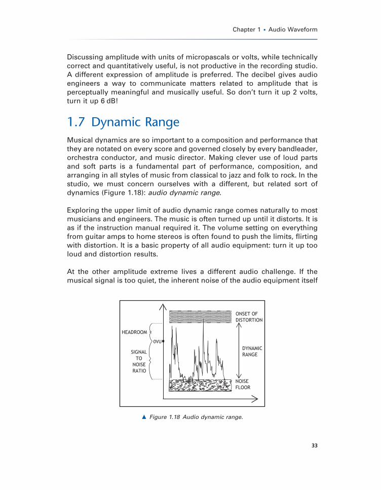
1.7 Dynamic RangeMusical dynamics are so important to a composition and performance that they are notated on every score and governed closely by every bandleader, orchestra conductor, and music director. Making clever use of loud parts and soft parts is a fundamental part of performance, composition, and arranging in all styles of music from classical to jazz and folk to rock. In the studio, we must concern ourselves with a different, but related sort of dynamics (Figure 1.18): audio dynamic range.

Exploring the upper limit of audio dynamic range comes naturally to most musicians and engineers. The music is often turned up until it distorts. It is as if the instruction manual required it. The volume setting on everything from guitar amps to home stereos is often found to push the limits, fl irting with distortion. It is a basic property of all audio equipment: turn it up too loud and distortion results.

At the other amplitude extreme lives a different audio challenge. If the musical signal is too quiet, the inherent noise of the audio equipment itself

� Figure 1.18 Audio dynamic range.



34

becomes audible and possibly distracting. Cassette tapes with their characteristic hiss and LPs with their crackles and rumble demonstrate the challenge that a noise fl oor presents. In fact, all audio equipment has a noise fl oor — equalizers, compressors, microphones, and even patch cables. Yes, even a cable made of pure gold, manufactured in zero gravity during the winter solstice of a leap year, costing half a year’s salary, will still have a noise fl oor, however faint.

A constant part of the recording craft then is using all these pieces of audio equipment in that safe amplitude zone, above the noise fl oor but below the point at which distortion begins. That safe zone is, in fact, the audio dynamic range. It defi nes and, using decibels, quantifi es the range of usable am-plitude between the noise a piece of gear makes and the level at which the piece of equipment starts to distort.

The target in between these two extremes is typically labeled zero VU. 0 VU is a nominal level for a signal through a piece of equipment. At 0 VU, the music gets through well above the self-noise of the equipment, but safely under the point where it starts to distort.

If we recorded pure sine waves for a living, we would raise the signal amplitude up just to the point of distortion, back off a smidge in level, and hit record. Thankfully, musical waveforms are nothing like sine waves. The amplitude of a musical waveform races wildly up and down due to both the character of the particular musical instrument and the way it is being played. Musical instruments lack the amplitude predictability of a sinusoid.

Some signals are more predictable than others. Electric guitars amps cranked to the limit have very little dynamic range. Many guitar sessions fi nd the engineer recording the way Nigel does, with the amp set to 11. Many (but not all) guitar amps sound best when they are cranked to within inches of their lives. This leaves no room for audio peaks to get through at a higher level. The meters on the mixing console and the multitrack recorder simply zip up to 0 VU at the downbeat, and then barely move until the end of the song. Chugga chugga crunch Ch-Chugga. Chugga chugga crunch Ch-Chugga. The meters do not budge until the guitarist stops playing. Crunchy rhythm rock-and-roll guitars are a case study in limited dynamic range.

Percussion, on the other hand, can be a complicated pattern of hard hits and delicate taps. Such an instrument is a challenge to record well, presenting extremely wide and diffi cult to predict dynamic range.



35

Every instrument offers its own complicated dynamics. The musical dynamic range of the instrument must somehow be made to fi t within the audio dynamic range of the studio’s equipment. Otherwise, the listeners are going to hear distortion, noise, or both.

Accommodating the unpredictability of all musical events, we record at a level well below the point where distortion begins. The amplitude “distance” (expressed in decibels) between the target operating level and the onset of distortion is called headroom. This provides the engineer a safety cushion, absorbing the musical dynamics of the instrument recorded without exceeding the audio dynamic range of the gear used to capture the recording.

The relative level of the noise fl oor compared to 0 VU, again expressed in decibels, is the signal-to-noise ratio. It quantifi es the level of the noise, relative to the nominal signal level. The trick, of course, is to send the audio signal through at a level well above the noise fl oor so that listeners will not even hear that hiss, hum, grit, and gunk that might be lurking low in the piece of equipment.

Making effective use of dynamic range infl uences how audio engineers record to any format, from analog tape to digital hard disk. It also governs the levels used when sending audio through a compressor, delay, reverb, or any other type of audio equipment. It is a constant tradeoff of noise at low amplitudes versus distortion at high amplitudes.

1.8 Sound MisconceptionsWith a more thorough understanding of the audio waveform, common errors in understanding and judgment can be avoided.

1.8.1 MISTAKING THE MESSAGE FOR THE MEDIUM

The transmission of sound from a source to a receiver does not require the delivery of air particles from the sound-making object to the listener. Sound waves propagate from the source to the receiver. The actual carrying medium — the air — does not. The springiness of air ensures that as the sound source drives the air, its infl uence spreads outward. The infl uence of air should not be confused with actual one-way motion of air. When a loudspeaker cone sends music towards a listener, it does not do so by sending a steady breeze of air into the person’s face. The pressure wave propagates; the air essentially stays put.



36

During the sound event, the air molecules stay in the same general space, moving about in a cloud as molecules are wont to do. As the pressure wave passes, these constantly moving gas particles are squeezed together and pulled apart slightly by the approach and retreat of neighboring air molecules or the vibration of the sound-producing instrument. After the sound wave has departed, the air molecules return to their original approximate locations.

Humans listen to the message carried by air. There is no reason to be particularly interested in any specifi c air particles themselves.

1.8.2 DON’T PICTURE THESE SKETCHES

The actual motion of the air particles associated with sound is in the same direction as the propagating sound wave itself. A wave propagating left to right causes the brief, organized jiggle, left and right, of air particles as the compression/rarefaction cycle occurs.

When the motion of the particles is in the same direction as the propagation of the wave, it is classifi ed a longitudinal wave. Sound does not belong to the slightly more intuitive family of waves known as transverse waves. Transverse waves have particle motion perpendicular to the wave motion. Making waves in water or snapping a rope demonstrates transverse waves. Toss the proverbial pebble in the allegorical still pond, and the vertical disruption of water ripples horizontally outward. Up and down motion of the end of a rope triggers a wave of up and down motion that is transmitted through the length of the rope. This seemingly insignifi cant fact — sound waves are longitudinal — causes some headaches when describing sound and has lead many an audio enthusiast into confusion.

Consider sound propagating from a loudspeaker toward a listener. Is the sound curving back and forth, up and down, as it heads horizontally from the speaker to the ears? No, it most defi nitely is not. For the sound heading from a loudspeaker to a listener in the same horizontal plane, there is nothing up and down about it. When sound propagates horizontally, the most interesting motion of the air particles is horizontal too. It might be sketched as a wave curving up and down, but the air particles in fact move only side to side.

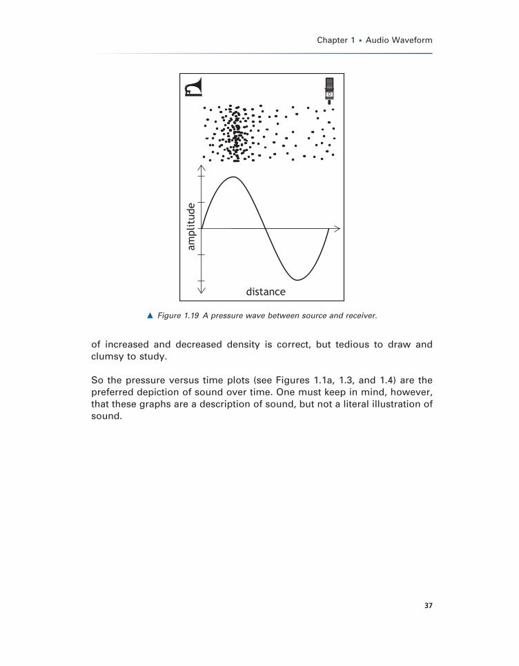
We resort to drawing up and down lines because it is too diffi cult to draw it literally (Figure 1.19). The clouds of air particles gathering into patterns



37

of increased and decreased density is correct, but tedious to draw and clumsy to study.

So the pressure versus time plots (see Figures 1.1a, 1.3, and 1.4) are the preferred depiction of sound over time. One must keep in mind, however, that these graphs are a description of sound, but not a literal illustration of sound.

� Figure 1.19 A pressure wave between source and receiver.


audio waveform - recordingologyrecordingology.com/.../soundfx_ch01_audiowaveform.pdfsound fx...

Documents