Submitted 28 January 2016Accepted 21 May 2016Published 27 June 2016

Corresponding authorGiovany Vega,aleph.omega@gmail.com

Academic editorAbhishek Kumar

Additional Information andDeclarations can be found onpage 19

DOI 10.7717/peerj-cs.70

Copyright2016 Vega et al.

Distributed underCreative Commons CC-BY 4.0

OPEN ACCESS

Audio segmentation using Flattened LocalTrimmed Range for ecological acousticspace analysisGiovany Vega1, Carlos J. Corrada-Bravo2 and T. Mitchell Aide3

1Department of Mathematics, University of Puerto Rico-Rio Piedras, San Juan, Puerto Rico, United States2Department of Computer Science, University of Puerto Rico-Rio Piedras, San Juan, Puerto Rico, United States3Department of Biology, University of Puerto Rico-Rio Piedras, San Juan, Puerto Rico, United States

ABSTRACTThe acoustic space in a given environment is filled with footprints arising from threeprocesses: biophony, geophony and anthrophony. Bioacoustic research using passiveacoustic sensors can result in thousands of recordings. An important componentof processing these recordings is to automate signal detection. In this paper, wedescribe a new spectrogram-based approach for extracting individual audio events.Spectrogram-based audio event detection (AED) relies on separating the spectrograminto background (i.e., noise) and foreground (i.e., signal) classes using a thresholdsuch as a global threshold, a per-band threshold, or one given by a classifier. Thesemethods are either too sensitive to noise, designed for an individual species, or requireprior training data. Our goal is to develop an algorithm that is not sensitive to noise,does not need any prior training data and works with any type of audio event. To dothis, we propose: (1) a spectrogram filtering method, the Flattened Local TrimmedRange (FLTR) method, which models the spectrogram as a mixture of stationary andnon-stationary energy processes and mitigates the effect of the stationary processes,and (2) an unsupervised algorithm that uses the filter to detect audio events. Wemeasured the performance of the algorithm using a set of six thoroughly validatedaudio recordings and obtained a sensitivity of 94% and a positive predictive valueof 89%. These sensitivity and positive predictive values are very high, given that thevalidated recordings are diverse and obtained from field conditions. The algorithm wasthen used to extract audio events in three datasets. Features of these audio events wereplotted and showed the unique aspects of the three acoustic communities.

Subjects Bioinformatics, Computational BiologyKeywords Audio event detection, Flattened Local Trimmed Range, Bioacoustic

INTRODUCTIONThe acoustic space in a given environment is filled with footprints of activity. Thesefootprints arise as events in the acoustic space from three processes: biophony, or thesound species make (e.g., calls, stridulation); geophony, or the sound made by differentearth processes (e.g., rain, wind); and anthrophony, or the sounds that arise from humanactivity (e.g., automobile or airplane traffic) (Krause, 2008). The field of Soundscape Ecologyis tasked with understanding and measuring the relation between these processes and theiracoustic footprints, as well as the total composition of this acoustic space (Pijanowski et al.,2011). Acoustic environment research depends more and more on data acquired through

How to cite this article Vega et al. (2016), Audio segmentation using Flattened Local Trimmed Range for ecological acoustic space analy-sis. PeerJ Comput. Sci. 2:e70; DOI 10.7717/peerj-cs.70

passive sensors (Blumstein et al., 2011; Aide et al., 2013) because recorders can acquiremore data than is possible manually (Parker III, 1991; Catchpole & Slater, 2003; Remsen,1994), and these data provide better results than traditional methods (Celis-Murillo, Deppe& Ward, 2012; Marques et al., 2013).

Currently, most soundscape analysis focus on computing indices for each recordingin a given dataset (Towsey et al., 2014), or on plotting and aggregating the raw acousticenergy (Gage & Axel, 2014). An alternative approach is to use each individual acousticevent as the base data and aggregate features computed from these events, but up untilnow, it has been difficult to accurately extract individual acoustic events from recordings.

We define an acoustic event as a perceptual difference in the audio signal that is indicativeof some activity. While being a subjective definition, this perceptual difference can bereflected in transformations of the signal (e.g., a dark spot in a recording’s spectrogram).

Normally, to use individual acoustic events as base data, a manual acoustic eventextraction is performed (Acevedo et al., 2009). This is usually done as a first step to buildspecies classifiers, and can be made very accurately. By using an audio visualization andannotation tool, an expert is able to draw a boundary around an acoustic event; however,this method is very time-consuming, is specific to a set of acoustic events and it is not easilyscalable for large datasets (e.g., >1000 minutes of recorded audio), thus an automateddetection method could be very useful.

Acoustic event detection (AED) has been used as a first step to build species classifiersfor whales, birds and amphibians (Popescu et al., 2013; Neal et al., 2011; Aide et al., 2013).Most AED approaches rely on using some sort of thresholding to binarize the spectrograminto background (i.e., noise) and foreground (i.e., signal) classes. Foreground spectrogramcells satisfying some contiguity constraint are then joined into a single acoustic event. Somemethods use a global threshold (Popescu et al., 2013), or a per-band threshold (Brandes,Naskrecki & Figueroa, 2006; Aide et al., 2013), while others train a species-specific classifierto perform the thresholding (Neal et al., 2011; Briggs, Raich & Fern, 2009). In Towsey etal. (2012) the authors reduce the noise in the spectrogram by using a 2D Wiener filterand removing modal intensity on each frequency band before applying a global threshold,but the threshold and parameters used in the AED tended to be species specific. Ratherthan using a threshold approach, Briggs et al. (2012) trained a classifier to label each cellin the spectrogram as sound or noise. These methods are either too sensitive to noise, arespecialized to specific species, require prior training data or require prior knowledge fromthe user. What is needed is an algorithm that works for any recording, is not targeted toa specific type of acoustic event, does not need any prior training data, is not sensitive tonoise, is fast and requires as little user intervention as possible.

In this article we propose a spectrogram filtering method, the Flattened Local TrimmedRange (FLTR) method, and an unsupervised algorithm that uses this filter for detectingacoustic events. Thismethod filters the spectrogrambymodeling it as amixture of stationaryand non-stationary energy processes, and mitigates the effect of the stationary processes.The detection algorithm applies FLTR to the spectrogram and proceeds to threshold itglobally. Afterward, each contiguous region above the threshold line is considered anindividual acoustic event.

Vega et al. (2016), PeerJ Comput. Sci., DOI 10.7717/peerj-cs.70 2/21

Figure 1 Flow diagram showing the workflow followed in this article. Recordings are filtered usingFLTR, then thresholded. Contiguous cells form each acoustic event. In step 1, we validate the extractedevents. In step 2, we compute features for each event and plot them. Acoustic events from one of the plot-ted regions are then sampled and cataloged.

We are interested in detecting automatically all acoustic events in a set of recordings. Assuch, this method tries to remove all specificity by design. Because of this, this method canwork as a form of data reduction. As a first step, this transforms the acoustic data into aset of events that can later feed further analysis.

The presentation of the article follows the workflow in Fig. 1: given a set of recordings,we compute the spectrogram for each one, then the FLTR is computed, a global thresholdis applied and, finally, we proceed to extract the acoustic events. These acoustic events arecompared with manually labeled acoustic events to determine the precision and accuracyof the automated process. We then applied the AEDmethodology to recordings from threedifferent sites. Features of the events were calculated and plotted to determine uniqueaspects of each site. Finally, events within a region of high acoustic activity were sampledto determine the sources of these sounds.

THEORYAudio spectrogramThe spectrogram of an audio recording separates the power in the signal into frequencycomponents in a short time window along a much longer time dimension (Fig. 2A). Thespectrogram is defined as the magnitude component of a Short Time Fourier Transform(STFT) on the audio data and it can be viewed as a time-frequency representation of themagnitude of the acoustic energy. This energy gets spread over distinct frequency bins as it

Vega et al. (2016), PeerJ Comput. Sci., DOI 10.7717/peerj-cs.70 3/21

Figure 2 FLTR steps. (A) An audio spectrogram. Color scale is in dB. (B) A band flattened spectrogram.(C) Local Trimmed Range (20× 20 window). (D) Thresholded image.

changes over time. Thus, providing a way of analyzing audio not just as a linear sequenceof samples, but as an evolving distribution, where each acoustic event is rendered as highenergy magnitudes in both time and frequency.

We represent a given spectrogram as a function S(t ,f ), where 0≤ t <τ and 0≤ t <ηare the time and frequency coordinates, bounded by τ , the number of audio frames givenby the STFT and η, the number of frequency bins in the transform.

Vega et al. (2016), PeerJ Comput. Sci., DOI 10.7717/peerj-cs.70 4/21

The Flattened Local Trimmed RangeThe first step in detecting acoustic events in the spectrogram requires creating the FlattenedLocal Trimmed Range (FLTR) image. Once we have the spectrogram, creating the FLTRrequires two steps: (1) flattening the spectrogram and (2) computing the local trimmedrange (Figs. 2B–2C). This image is produced by modeling the spectrogram as a sum ofdifferent energetic processes, along with some assumptions on the distributions of theacoustic events, and a proposed solution that takes advantage of the model to separate theenergetic processes.

Modeling the spectrogramWe model the spectrogram Sdb(t ,f ) as a sum of different energetic processes:

Sdb(t ,f )= b(f )+ε(t ,f )+n∑

i=1

Ri(t ,f )Ii(t ,f ), (1)

where b(f ) is a frequency-dependent process that is taken as constant in time, while ε(t ,f )is a process that is stationary in time and frequency with 0-mean, 0-median, and somescale parameter, and Ri(t ,f ) is a set of non-zero-mean localized energy processes thatare bounded by their support functions Ii

(t ,f), for 1≤ i≤ n. An interpretation for these

energetic processes is that b(f ) corresponds to a frequency-dependent near-constant noise,ε(t ,f ) corresponds to a global noise process with a symmetric distribution and the Ri(t ,f )are our acoustic events, of which there are n.

In this model, we assume that the set of localized energy processes has four properties:A1 The localized energy processes are mutually exclusive and are not adjacent. That is, no

two localized energy processes share in the same (t ,f ) coordinate, nor do they haveadjacent coordinates. Thus, ∀1≤ i,j ≤ n,i 6= j,0≤ t <τ,0≤ f <η, we have:

Ii(t ,f)Ij(t ,f)= 0

Ii(t+1,f

)Ij(t ,f)= 0

Ii(t−1,f

)Ij(t ,f)= 0

Ii(t ,f +1

)Ij(t ,f)= 0

Ii(t ,f −1

)Ij(t ,f)= 0.

This can be done without loss of generality. If two such localized processes existed, wecan just consider their union as one.

A2 The regions of localized energy processes dominate the energy distribution in thespectrogram on each given band. That is, ∀0≤ t1,t2<τ , 0≤ f <η, we have:

ε(t1,f )+b(f )≤ ε(t2,f )+b(f )+n∑

i=1

Ii(t2,f

)Ri(t2,f ).

A3 The proportion of samples within a localized energy processes in a given frequencyband, denoted as ρ(f ), is less than half the samples in the entire frequency band. That

Vega et al. (2016), PeerJ Comput. Sci., DOI 10.7717/peerj-cs.70 5/21

is, ∀0≤ f <η, we have:

ρ(f )=1τ

τ∑t=0

n∑i=1

Ii(t ,f)< .5.

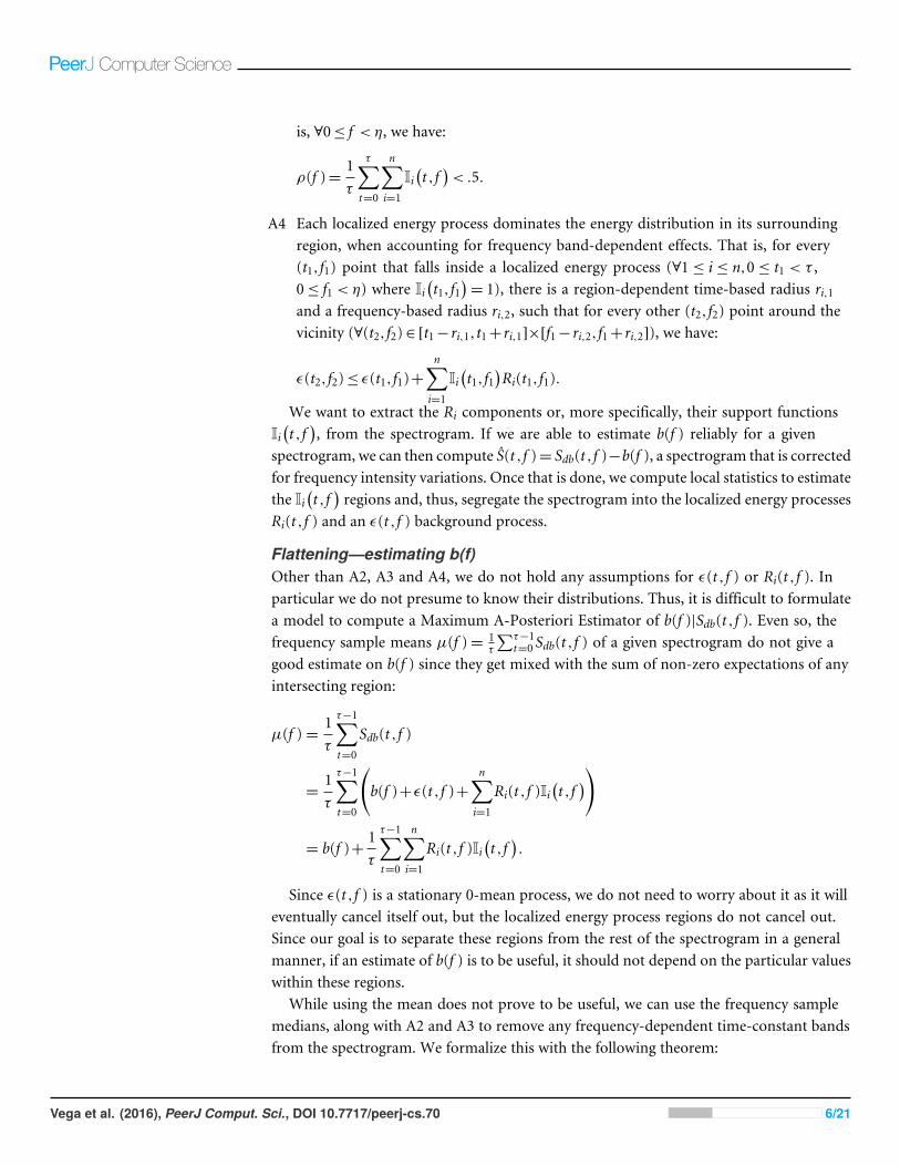
A4 Each localized energy process dominates the energy distribution in its surroundingregion, when accounting for frequency band-dependent effects. That is, for every(t1,f1) point that falls inside a localized energy process (∀1 ≤ i ≤ n,0 ≤ t1 < τ ,0≤ f1 < η) where Ii

(t1,f1

)= 1), there is a region-dependent time-based radius ri,1

and a frequency-based radius ri,2, such that for every other (t2,f2) point around thevicinity (∀(t2,f2)∈ [t1− ri,1,t1+ ri,1]×[f1− ri,2,f1+ ri,2]), we have:

ε(t2,f2)≤ ε(t1,f1)+n∑

i=1

Ii(t1,f1

)Ri(t1,f1).

We want to extract the Ri components or, more specifically, their support functionsIi(t ,f), from the spectrogram. If we are able to estimate b(f ) reliably for a given

spectrogram, we can then compute S(t ,f )= Sdb(t ,f )−b(f ), a spectrogram that is correctedfor frequency intensity variations. Once that is done, we compute local statistics to estimatethe Ii

(t ,f)regions and, thus, segregate the spectrogram into the localized energy processes

Ri(t ,f ) and an ε(t ,f ) background process.

Flattening—estimating b(f)Other than A2, A3 and A4, we do not hold any assumptions for ε(t ,f ) or Ri(t ,f ). Inparticular we do not presume to know their distributions. Thus, it is difficult to formulatea model to compute a Maximum A-Posteriori Estimator of b(f )|Sdb(t ,f ). Even so, thefrequency sample means µ(f )= 1

τ

∑τ−1t=0 Sdb(t ,f ) of a given spectrogram do not give a

good estimate on b(f ) since they get mixed with the sum of non-zero expectations of anyintersecting region:

µ(f )=1τ

τ−1∑t=0

Sdb(t ,f )

=1τ

τ−1∑t=0

(b(f )+ε(t ,f )+

n∑i=1

Ri(t ,f )Ii(t ,f))

= b(f )+1τ

τ−1∑t=0

n∑i=1

Ri(t ,f )Ii(t ,f).

Since ε(t ,f ) is a stationary 0-mean process, we do not need to worry about it as it willeventually cancel itself out, but the localized energy process regions do not cancel out.Since our goal is to separate these regions from the rest of the spectrogram in a generalmanner, if an estimate of b(f ) is to be useful, it should not depend on the particular valueswithin these regions.

While using the mean does not prove to be useful, we can use the frequency samplemedians, along with A2 and A3 to remove any frequency-dependent time-constant bandsfrom the spectrogram. We formalize this with the following theorem:

Vega et al. (2016), PeerJ Comput. Sci., DOI 10.7717/peerj-cs.70 6/21

Theorem 1. Let 0≤ f ≤ η be a frequency band in the spectrogram, with a proportion oflocalized energy processes given as ρ(f )= 1

τ

∑τt=0∑n

i=0Ii(t ,f), and a median m(f ). Assume

A2 and that ρ(f )< .5, then m(f ) depends only in the ε process and does not depend on anyof the localized energy processes Ri(t ,f ).

Proof. ρ(f ) is the proportion of energy samples in a given frequency band f that participatein a localized energy process. Then, ρ(f )< .5 implies that less than 50% of the energysamples do so. This means that a 1−ρ(f )> .5 proportion of the samples in band f aredescribed by the equation Sdb(t ,f )= b(f )+ε(t ,f ). A2 implies that the lower half of thepopulation is within this 1−ρ(f ) proportion, along with the frequency band medianm(f ).Thus m(f ) does not depend on the localized energy processes Ri(t ,f ). �

Thus, assuming A2 and A3, m(f ) gives an estimator whose bias is limited by the rangeof the ε process and is completely unaffected by the Ri processes. Furthermore, as ρ(f )approaches 0, m(f ) approaches b(f ).

We use the term band flattening to refer to the process of subtracting the b(f ) componentfrom Sdb(t ,f ). Thus we call S(t ,f )= Sdb(t ,f )−m(f ) the band flattened spectrogramestimate of Sdb(t ,f ). Figure 2B shows the output from this flattening procedure. As canbe seen, this procedure removes any frequency-dependent time-constant bands in thespectrogram.

Estimating Ii (t,f )We can use the band flattened spectrogram S(t ,f ) to further estimate the Ii

(t ,f)regions,

since:

S(t ,f )≈ Sdb(t ,f )−b(f )

= ε(t ,f )+n∑

i=1

Ri(t ,f )Ii(t ,f).

We do this by computing the local α-trimmed range Raα{S}. That is, given some0≤α < 50, and some r > 0, for each (t ,f ) pair, we compute:

Raα{S}(t ,f )= P100−α(Sner (t ,f ))−Pα(Sner (t ,f )),

where Pα(·) is the α percentile statistic, and Sner (t ,f ) is the band flattened spectrogram, withits domain restricted to a square neighborhood of range r (in time and frequency) aroundthe point (t ,f ).

Assuming A4, the estimator would give small values for neighborhoods without localizedenergy processes, but would peak around the borders of any such process. This statisticcould then be thresholded to compute estimates of these borders and an estimate ofthe support functions Ii

(t ,f). Figure 2C shows the local trimmed range of a flattened

spectrogram image. As can be seen, areas with acoustic events have a higher local trimmedrange, while empty areas have a lower one.

Vega et al. (2016), PeerJ Comput. Sci., DOI 10.7717/peerj-cs.70 7/21

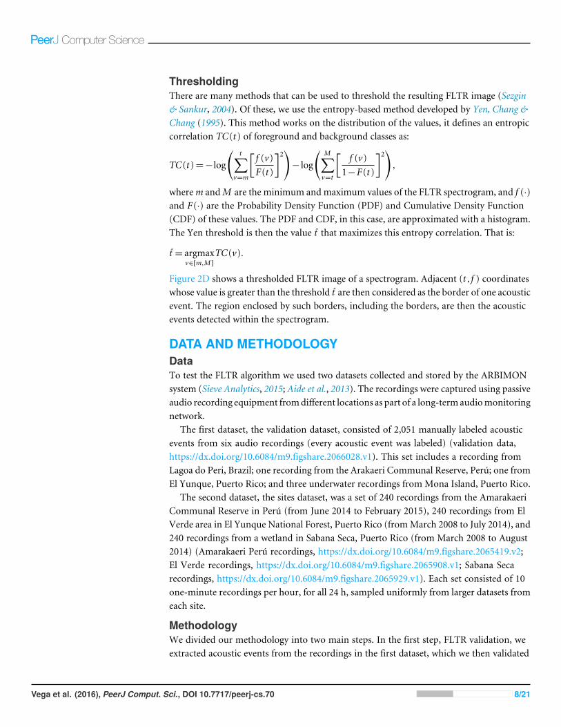
ThresholdingThere are many methods that can be used to threshold the resulting FLTR image (Sezgin& Sankur, 2004). Of these, we use the entropy-based method developed by Yen, Chang &Chang (1995). This method works on the distribution of the values, it defines an entropiccorrelation TC(t ) of foreground and background classes as:

TC(t )=−log

( t∑v=m

[f (v)F(t )

]2)− log

( M∑v=t

[f (v)

1−F(t )

]2),

wherem andM are the minimum andmaximum values of the FLTR spectrogram, and f (·)and F(·) are the Probability Density Function (PDF) and Cumulative Density Function(CDF) of these values. The PDF and CDF, in this case, are approximated with a histogram.The Yen threshold is then the value t that maximizes this entropy correlation. That is:

t = argmaxv∈[m,M ]

TC(v).

Figure 2D shows a thresholded FLTR image of a spectrogram. Adjacent (t ,f ) coordinateswhose value is greater than the threshold t are then considered as the border of one acousticevent. The region enclosed by such borders, including the borders, are then the acousticevents detected within the spectrogram.

DATA AND METHODOLOGYDataTo test the FLTR algorithm we used two datasets collected and stored by the ARBIMONsystem (Sieve Analytics, 2015; Aide et al., 2013). The recordings were captured using passiveaudio recording equipment fromdifferent locations as part of a long-termaudiomonitoringnetwork.

The first dataset, the validation dataset, consisted of 2,051 manually labeled acousticevents from six audio recordings (every acoustic event was labeled) (validation data,https://dx.doi.org/10.6084/m9.figshare.2066028.v1). This set includes a recording fromLagoa do Peri, Brazil; one recording from the Arakaeri Communal Reserve, Perú; one fromEl Yunque, Puerto Rico; and three underwater recordings from Mona Island, Puerto Rico.

The second dataset, the sites dataset, was a set of 240 recordings from the AmarakaeriCommunal Reserve in Perú (from June 2014 to February 2015), 240 recordings from ElVerde area in El Yunque National Forest, Puerto Rico (fromMarch 2008 to July 2014), and240 recordings from a wetland in Sabana Seca, Puerto Rico (from March 2008 to August2014) (Amarakaeri Perú recordings, https://dx.doi.org/10.6084/m9.figshare.2065419.v2;El Verde recordings, https://dx.doi.org/10.6084/m9.figshare.2065908.v1; Sabana Secarecordings, https://dx.doi.org/10.6084/m9.figshare.2065929.v1). Each set consisted of 10one-minute recordings per hour, for all 24 h, sampled uniformly from larger datasets fromeach site.

MethodologyWe divided our methodology into two main steps. In the first step, FLTR validation, weextracted acoustic events from the recordings in the first dataset, which we then validated

Vega et al. (2016), PeerJ Comput. Sci., DOI 10.7717/peerj-cs.70 8/21

against the manually labeled acoustic events. In the second step, site acoustic eventvisualization, we extracted the acoustic events from the second dataset, computed featurevectors for each event and plotted them. The recording spectrograms were computed usinga Hann window function of 512 audio samples and an overlap of 256 samples.

FLTR validationWe used the FLTR algorithm with a 21 × 21 window and α= 5 to extract the acousticevents and compared them with the manually labeled acoustic events.

For the validation, we used two comparison methods, the first is based on a basicintersection test between the automatically detected and the manually labeled events’bounds, and the second one is based on an overlap percent. For each manual label anddetection event pair, we defined the computed overlap percent as the ratio of the area oftheir intersection and the area of their union:

O(L,D)=A(L∩D)A(L∪D)

,

where L is a manually labeled event, D is a automatically detected event area, and A(L∩D)and A(L∪D) are the area of the intersection and the union of their respective bounds.

On the first comparison method, for each acoustic event whose bounds intersected thebounds of a manually labeled acoustic event, we registered it as a detected acoustic event.For each detected event whose bounds did not intersect any manually labeled acousticevents, we registered it as detected, but without an acoustic event. On the other hand, themanually labeled acoustic events that did not intersect any detected acoustic event wereregistered as undetected acoustic events.

The secondmethod followed a similar path as the first, but it requires an overlap percentof at least 25%. For each acoustic event whose overlap percent with a manually labeledacoustic event was greater than or equal to 25%, we registered it as a detected acousticevent. For each detected event that did not have any manually labeled acoustic events withan overlap percent of at least 25%, we registered it as detected, but without an acousticevent. On the other hand, the manually labeled acoustic events that did not have an overlappercent of at least 25% with any detected acoustic event were registered as undetectedacoustic events.

These data were used to create a confusion matrix to compute the FLTR algorithm’ssensitivity and positive predictive value for each method. The sensitivity is computed as theratio of the number of manually labeled acoustic events that were automatically detected(true positives) over the total count of manually labeled acoustic events (true positives andfalse negatives).

Sensitivity=True Positives

True Positives+False Negatives.

This measurement reflects the percent of detected acoustic events that were present in therecording.

The positive predictive value is computed as the ratio of the number of manually labeledacoustic events that were automatically detected (true positives) over the total count of

Vega et al. (2016), PeerJ Comput. Sci., DOI 10.7717/peerj-cs.70 9/21

detected acoustic events (true positives and false positives).

Positive Predictive Value=True Positives

True Positives+False Positives.

This measurement reflects the percent of real acoustic events among the set of detectedacoustic events.

FLTR applicationAs with the FLTR validation step, we used the FLTR algorithm with a 21×21 window andα= 5 to extract the acoustic events in each of the recording samples in the second dataset,which we then converted into feature vectors.

The variables computed for each extracted acoustic event Ri were:

tod Time of Day. Hour in which the recording from this acoustic event was taken.bw Bandwidth. Length of the acoustic event in Hertz. That is, given Fi={f |∃t ,Ii

(t ,f)=

1}, the bandwidth is defined as:

bwi=max(Fi)−min(Fi). (2)

dur Duration. Length of the acoustic event in seconds. That is, given Ti={t |∃f ,Ii(t ,f)=

1}, the duration is defined as:

duri=max(Ti)−min(Ti). (3)

y_max Dominant Frequency. The frequency at which the acoustic event attains itsmaximum power:

y_maxi= arg maxf

(maxt

Ii(t ,f)S(t ,f )

). (4)

cov Coverage Ratio. The ratio between the area covered by the detected acoustic eventand the area detected by the bounds:

covi=

∑t ,f Ii

(t ,f)

duribwi. (5)

Using these features, we generate a log-density plot matrix for all pairwise combinationsof the features for each site. The plots in the diagonal are log histograms of the columnfeature.

We measured the information content of each feature pair by computing their jointentropy H :

H =1

N1N2

N1∑i=1

N2∑j=1

hi,j log2hi,j,

where log2 is the base 2 logarithm, hi,j is the number of events in the (i,j)th bin of thejoint histogram, and N1 and N2 are the number of bins of each variable in the histogram.A higher value of H means a higher information content.

Vega et al. (2016), PeerJ Comput. Sci., DOI 10.7717/peerj-cs.70 10/21

Table 1 Validation dataset confusionmatrix under simple intersection test. Confusion matrix basedon the FLTR results of the six recordings from the validation dataset using the simple intersection test.Notice that the algorithm only produces detection events. We do not provide a result for true negatives asany arbitrary number of true negative examples could be made, thus skewing the data.

Acoustic event No acoustic event Total

Detected 1,922 245 2,167Not detected 129 – 129Total 2,051 245 2,296

Sensitivity 1,922/2,051 94%Positive predictive value 1,922/2,167 89%

We also focused our attention on areas with a high and medium count of detectedacoustic events (log of detected events greater than 6 and 3.5, respectively). As an example,we selected an area of interest in the feature space of the Sabana Seca dataset (i.e., a visualcluster in the bw vs. y_max plot). We sampled 50 detected acoustic events from the areaand categorized them manually.

RESULTSFLTR validationUnder the simple intersection test, out of 2,051 manually labeled acoustic events, 1,922were detected (true positives), and 129 were not (Table 1). Of the 2,167 detected acousticevents, 1,922 were associated with manually labeled acoustic events (true positives), and245 were not (false negatives). This resulted in a sensitivity of 94% and a positive predictivevalue of 89%.

Under the overlap percentage test, out of 2,051 manually labeled acoustic events, 1,744were detected (true positives), and 307 were not (Table 2). Of the 2,167 detected acousticevents, 1,744 were associated with manually labeled acoustic events (true positives), and423 were not (false negatives). This resulted in a sensitivity of 85% and a positive predictivevalue of 80%.

Figure 3 shows the spectrograms of a sample of six acoustic events from the validationstep, alongwith their FLTR images. Figures 3A–3D aremanually labeled acoustic events thatwere detected. Figures 3E–3H are manually labeled acoustic events that were not detected.Figures 3I–3L are detected acoustic events that were not labeled. The FLTR images showhow the surrounding background gets filtered and the acoustic event stands above it.Figures 3F shows lower than threshold FLTR values, possibly due to the spectrogramflattening. FLTR values in Fig. 3H is too low to cross the threshold as well and Fig. 3I showsa detection of some low-frequency short lived audio noise.

FLTR applicationThe feature pairs with highest joint entropy in the plots of the Perú recordings are cov vs.y_max, y_max vs. tod and cov vs. tod with values of 9.37, 9.25 and 8.81 respectively (Fig. 4).The cov vs. y_max plot shows three areas of high event detection count at 2.4–4.6 kHz with

Vega et al. (2016), PeerJ Comput. Sci., DOI 10.7717/peerj-cs.70 11/21

Figure 3 Sample of the intersections of 6 acoustic events along with their FLTR image. (A–D) are man-ually labeled and detected, (E–H) are manually labeled but not detected detected, and (I–L) are detectedbut not manually labeled.

Table 2 Validation dataset confusionmatrix under overlap percentage test. Confusion matrix based onthe FLTR results of the six recordings from the validation dataset using the overlap percentage test. Noticethat the algorithm only produces detection events. We do not provide a result for true negatives as any ar-bitrary number of true negative examples could be made, thus skewing the data.

Acoustic event No acoustic event Total

Detected 1,744 423 2,167Not detected 307 — 307Total 2,051 423 2,296

Sensitivity 1,744/2,051 85%Positive predictive value 1,744/2,167 80%

Vega et al. (2016), PeerJ Comput. Sci., DOI 10.7717/peerj-cs.70 12/21

Figure 4 Amarakaeri, Perú, log density plot matrix of acoustic events extracted from 240 samplerecordings.Variables shown are time of day (tod), bandwidth (bw), duration (dur), dominant frequency(y_max) and coverage (cov). Note high H values for cov vs. y_max (9.37), y_max vs. tod (9.25) and cov vs.tod(8.81) .

84–100% coverage, 7.0–7.4 kHz with 88–100% coverage and 8.4–8.8 kHz with 84–100%coverage. Three areas of medium event detection count can be found at 12.8–14.9 kHzwith 68–90% coverage, 18.5–20.4 kHz with 59–90% coverage and one spanning the whole90–100% coverage band. The y_max vs. tod plot shows two areas of high event detectioncount from 5pm to 5am at 2.9–5.9 kHz and from 7pm to 4am at 9.6–10 kHz. Three areas ofmedium event detection count can be found at from 6pm to 5am at 17.6–20.9 kHz, from5pm to 5am at 15.7–10.5 kHz and one spanning the entire day at 7.5–10.5 kHz. The covvs. tod plot shows one area of high event detection count from 6pm to 5am with 84–100%coverage and another area of medium event detection count throughout the entire daywith 60–84% coverage from 6pm to 5am and with 77–100% coverage from 6am to 5pm.

The feature pairs with highest joint entropy in the plots of the El Verde recordings arecov vs. y_max, y_max vs. tod and cov vs. tod with values of 9.06, 9.03 and 8.84 respectively(Fig. 5). The cov vs. y_max plot shows two areas of high event detection count at 3.3–1.9 kHz

Vega et al. (2016), PeerJ Comput. Sci., DOI 10.7717/peerj-cs.70 13/21

Figure 5 El Verde, Puerto Rico, log density plot matrix of acoustic events extracted from 240 samplerecordings.Variables shown are time of day (tod), bandwidth (bw), duration (dur), dominant frequency(y_max) and coverage (cov). Note high Hn values for tod (0.98), cov (0.84) and y_max (0.83).

with 67–100% coverage and 1.4–0.8 kHz with 82–100% coverage. Three areas of mediumevent detection count can be found at 7.1–9.8 kHz with 59–98% coverage, 20.1–20.8 kHzwith 65–98% coverage and one spanning the whole 98–100% coverage band. The y_max vs.tod plot shows three areas of high event detection count from 6pm to 7am at 1.9–2.9 kHz,from 7pm to 6am at 1.0–1.4 kHz and one spanning the entire day at 0–0.5 kHz. Two areasof medium event detection count span the whole day, one at 3.5–5.1 kHz and anotherone at 6.1–9.9 kHz. Vertical bands of medium event detection count areas can be foundat 12am–5am, 7am, 10am–12pm, 3pm and 8pm. The cov vs. tod plot shows an area ofmedium event detection count spanning the entire day with 46–100% coverage, changingto 75–100% coverage from 1pm to 5pm. There seems to be a downward trending densityline on the upper left corner of the plot in y_max vs. bw.

The feature pairs with highest joint entropy in the plots of the Sabana Seca recordings arecov vs. y_max, y_max vs. tod and cov vs. tod with values of 8.71, 8.78 and 8.36 respectively(Fig. 6). The cov vs. y_max plot shows four areas of high event detection count at 0–0.2 kHz

Vega et al. (2016), PeerJ Comput. Sci., DOI 10.7717/peerj-cs.70 14/21

Figure 6 Sabana Seca, Puerto Rico, log density plot matrix of audio events extracted from 240 samplerecordings.Variables shown are time of day (tod), bandwidth (bw), duration (dur), dominant frequency(y_max) and coverage (cov). Note high Hn values for tod (0.96), cov (0.81) and y_max (0.8).

with 83–100% coverage, 1.3–1.8 kHz with 87–100% coverage, 4.6–5.5 kHz with 79–100%coverage and 7.0–7.9 kHz with 74–100% coverage. Areas of medium event detection countcan be found surrounding the areas of high event detection count. The y_max vs. tod plotshows four areas of high event detection count from 3pm to 7am at 6.8–8.1 kHz, from4pm to 7am at 4.5–5.5 kHz, from 5pm to 11pm at 1.3–4.1 kHz and from 8am to 9pm at0–0.4 kHz. Two areas of medium event detection count can be found from 1am to 7am at1.4–4.4 kHz and from 8am to 2pm at 3.7–9.4 kHz span the whole day, one at 3.5–5.1 kHzand another one at 6.1–9.9 kHz. The cov vs. tod plot shows an area of medium eventdetection count spanning the entire day with 69–100% coverage, changing to 47–100%coverage at 4pm–1am and 5am–6am.

Sampled areas of interestIn the Sabana Seca bw vs. y_max plot, there are five high event detection count areas(Fig. 7). We focus on the region with bandwidth between 700 Hz and 1,900 Hz, anddominant frequency between 2,650 Hz and 3,550 Hz.

Vega et al. (2016), PeerJ Comput. Sci., DOI 10.7717/peerj-cs.70 15/21

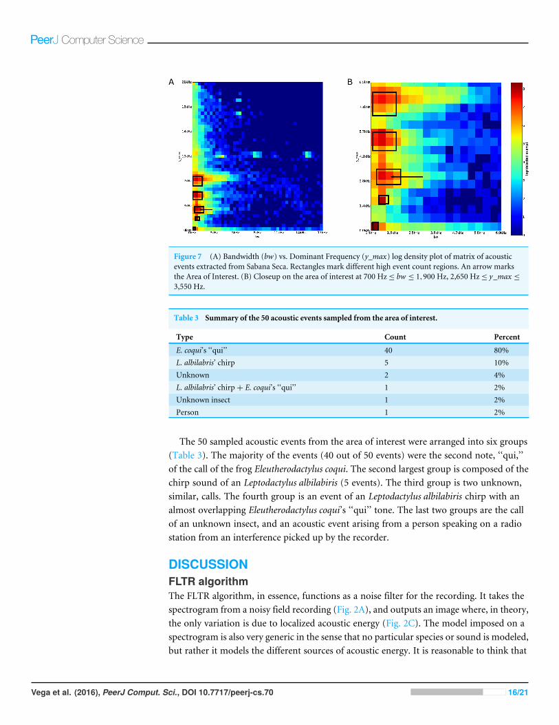
Figure 7 (A) Bandwidth (bw) vs. Dominant Frequency (y_max) log density plot of matrix of acousticevents extracted from Sabana Seca. Rectangles mark different high event count regions. An arrow marksthe Area of Interest. (B) Closeup on the area of interest at 700 Hz≤ bw ≤ 1,900 Hz, 2,650 Hz≤ y_max ≤3,550 Hz.

Table 3 Summary of the 50 acoustic events sampled from the area of interest.

Type Count Percent

E. coqui’s ‘‘qui’’ 40 80%L. albilabris’ chirp 5 10%Unknown 2 4%L. albilabris’ chirp+ E. coqui’s ‘‘qui’’ 1 2%Unknown insect 1 2%Person 1 2%

The 50 sampled acoustic events from the area of interest were arranged into six groups(Table 3). The majority of the events (40 out of 50 events) were the second note, ‘‘qui,’’of the call of the frog Eleutherodactylus coqui. The second largest group is composed of thechirp sound of an Leptodactylus albilabiris (5 events). The third group is two unknown,similar, calls. The fourth group is an event of an Leptodactylus albilabiris chirp with analmost overlapping Eleutherodactylus coqui’s ‘‘qui’’ tone. The last two groups are the callof an unknown insect, and an acoustic event arising from a person speaking on a radiostation from an interference picked up by the recorder.

DISCUSSIONFLTR algorithmThe FLTR algorithm, in essence, functions as a noise filter for the recording. It takes thespectrogram from a noisy field recording (Fig. 2A), and outputs an image where, in theory,the only variation is due to localized acoustic energy (Fig. 2C). The model imposed on aspectrogram is also very generic in the sense that no particular species or sound is modeled,but rather it models the different sources of acoustic energy. It is reasonable to think that

Vega et al. (2016), PeerJ Comput. Sci., DOI 10.7717/peerj-cs.70 16/21

any spectrogram is composed of these three components without a loss of generality: (1) afrequency-based noise level, (2) some diffuse energy jitter, and (3) specific, localized events.

The end product of the flattening step is a spectrogram with no frequency-basedcomponents (Fig. 2B). By using the frequency band medians we are able to stay ignorant ofthe nature of the short-term dynamics in the spectrogram while being able to remove anylong-term nuisance effects, such as (constant) background noise or a specific audio sensor’sfrequency response. Thus, we end up with a spectrogram that is akin to a flat landscapewith two components: (1) a roughness element (i.e., grass leaves) in the landscape and (2)a series of mounds, each corresponding to a given acoustic event. Due to this roughnesselement, a global threshold at this stage is ineffective. The local trimmed range however isable to enhance the contrast between the flat terrain and the mounds (Fig. 2C), enough todetect the mounds by using a simple global threshold (Fig. 2C). By using a Yen threshold,we maximize the entropy of both the background and foreground classes (Fig. 2D). In theend, the FLTR algorithm has the advantage of not trying to guess the distribution of theacoustic energy within the spectrogram, but rather it exploits robust statistics that workfor any distribution to separate these three modeled components.

From the simple intersection test, a sensitivity of 94% assures us that most of the acousticevents in a given recording will be extracted by the FLTR segmentation algorithm, while apositive predictive value of 89% assures us that if something is detected in the recording,it is most likely an acoustic event. Thus, this algorithm can confidently extract acousticevents from a given set of recordings.

From the coverage percentage test, a sensitivity of 85% assures us that most of theacoustic events in a given recording will be extracted by the FLTR segmentation algorithm,while a positive predictive value of 80% assures us that if something is detected in therecording, it is most likely an acoustic event. Thus, this algorithm can confidently extractacoustic events from a given set of recordings.

These performance statistics are obtained from a dataset of only six recordings. Becauseof this small recording size, biases that may occur due to correlations between acousticevents within a recording cannot be addressed. We tried to reduce this bias by selectingrecordings from very different environments. This limitation arises from the fact thatmanually annotating the acoustic events in a recording is very time consuming. Thus, alimiting factor on the sample size in the validation dataset is that the number of extractedacoustic events for each recording averages to 340 per recording (i.e., for six recordings,we have 2,051 manually labeled acoustic events in total).

The 21 × 21 window parameter was selected in an ad-hoc manner and corresponds toa square neighborhood of a maximum of 10 spectrogram cells around the central cell inthe local trimmed range computation step. This allows us to compare each value in thespectrogram to a local neighborhood of about 122 ms and 1.8 kHz in size (assuming asampling rate of 44,100, or 500 ms and 410 Hz for sampling rate of 10,000 Hz). The α= 5percentile was also selected ad-hoc. It corresponds to the local trimmed range computingthe difference between the 95% and 5% percentiles. This allows the window to containat least 5% percent of its content as low-valued outliers, and another 5% as high-valuedoutliers. While these parameter values provided good results, it is not know how optimal

Vega et al. (2016), PeerJ Comput. Sci., DOI 10.7717/peerj-cs.70 17/21

they are, nor how the sensitivity and positive predictive value would change if otherparameter values were used.

A3 implies that a recording needs to have unsaturated frequency bands (ρ(f )< .5) forthemethod towork efficiently. This assumption implies that Theorem 1 holds for frequencybands without intense constant chorus (ρ(f )≤ .5). However, as ρ(f ) approaches 1, thefrequency band median approaches the median of the aggregate localized energy processeson the frequency band. Thus, at least 50% of the values, more notably the highest values inthe aggregate localized energy processes, will always be above b(f ). Depending on factors,such as their size and remaining intensity, they could very well be detected. The degradationof the detection algorithm in relation to these assumptions, however, is still to be studied.

FLTR applicationIn all three sites, the plots with the most joint entropy were cov vs. y_max, y_max vs. todand cov vs. tod. cov measures how well a detection fits within a bounding box and canserve as a measure of the complexity of the event. This value changing across tod andy_max implies that the complexity of the detected event change across these features. Thehigh joint entropy of y_max vs. tod is expected, since each variable amounts to beinga location estimate: (tod is a location estimate in time while y_max in frequency) and,thus, subject to the randomness of when (in time) and where (in frequency) an acousticevent occurs. Interestingly, rather than being uniformly distributed, the acoustic eventsare non-randomly distributed, presumably reflecting the variation in acoustic activitythroughout the day. These tod vs. y_max plots present a temporal soundscape, whichprovide us with insights into how the acoustic space is partitioned in time and frequencyin each ecosystem. For example, in the Sabana Seca and El Verde plots, there is a cleardifference in acoustic event density between day time and night time. This correlateswith the activity of amphibian vocalizations during the night in these sites (Ríos-López &Villanueva-Rivera, 2013; Villanueva-Rivera, 2014).

An interesting artifact is a downward trending density line that appears on the upper leftcorner of the plot in y_max vs. bw in Fig. 5. A least squares fit to this line gives the equation−0.93X+21.5 kHz, which is close to the maximum frequency of the recordings from ElVerde site (these recordings have a sampling rate of 44,100). This artifact seems to arisebecause the upper boundary of a detected event and bw are constrained to be below thismaximum frequency and, for low bw values, y_max is to be close to the upper boundaryof the detected event.

Another useful application of the FLTR methodology is to sample specific regions ofactivity to determine the source of the sounds. In the sampled area of interest from SabanaSeca, approximately 80% of the sampled of the events were a single note of a call of E. coqui(40 events), and around 10% were the chirp of L. albilabris (5 events). This demonstrateshow the methodology can be used to annotate regions of peak activity in a soundscape.

Using the confusion matrix in Table 1 as a ruler, we could estimate that around 94% ofthe acoustic events were detected and that they conform around 89% of the total amountof detected events.

Vega et al. (2016), PeerJ Comput. Sci., DOI 10.7717/peerj-cs.70 18/21

CONCLUSIONThe FLTR algorithm uses a sound spectrogram model. Using robust statistics, it is ableto exploit the spectrogram model without assuming any specific energy distributions.Coupled with the Yen threshold, we are able to extract acoustic events from recordingswith high levels of sensitivity and precision.

Using this algorithm, we are able to explore the acoustic environment using acousticevents as base data. This provides us with an excellent vantage point where any featurecomputed from these acoustic events can be explored, for example the time of day vs.dominant frequency distribution of an acoustic environment (i.e., a temporal soundscape)down to the level of the individual acoustic events composing it. As a tool, the FLTRalgorithm, or any improvements thereof, have the potential of shifting the paradigm fromusing recordings to acoustic events as base data for ecological acoustic research.

ADDITIONAL INFORMATION AND DECLARATIONS

FundingThe authors received no funding for this work.

Competing InterestsThe authors declare there are no competing interests.

Author Contributions• Giovany Vega conceived and designed the experiments, performed the experiments,analyzed the data, contributed reagents/materials/analysis tools, wrote the paper,prepared figures and/or tables, performed the computation work, reviewed draftsof the paper.• Carlos J. Corrada-Bravo and T. Mitchell Aide conceived and designed the experiments,analyzed the data, contributed reagents/materials/analysis tools, reviewed drafts of thepaper.

Data AvailabilityThe following information was supplied regarding data availability:

Figures:https://dx.doi.org/10.6084/m9.figshare.2063871https://dx.doi.org/10.6084/m9.figshare.2063877https://dx.doi.org/10.6084/m9.figshare.2063880https://dx.doi.org/10.6084/m9.figshare.2063883https://dx.doi.org/10.6084/m9.figshare.2063895https://dx.doi.org/10.6084/m9.figshare.2063901Validation data:https://dx.doi.org/10.6084/m9.figshare.2066028Other data:https://dx.doi.org/10.6084/m9.figshare.2065419

Vega et al. (2016), PeerJ Comput. Sci., DOI 10.7717/peerj-cs.70 19/21

https://dx.doi.org/10.6084/m9.figshare.2065908https://dx.doi.org/10.6084/m9.figshare.2065929Implementation:https://github.com/g-i-o-/fltrlib.git.

REFERENCESAcevedoMA, Corrada-Bravo CJ, Corrada-Bravo H, Villanueva-Rivera LJ, Aide

TM. 2009. Automated classification of bird and amphibian calls using machinelearning: a comparison of methods. Ecological Informatic 4(4):206–214DOI 10.1016/j.ecoinf.2009.06.005.

Aide TM, Corrada-Bravo C, Campos-Cerqueira M, Milan C, Vega G, Alvarez R. 2013.Real-time bioacoustics monitoring and automated species identification. PeerJ1:e103 DOI 10.7717/peerj.103.

Blumstein DT, Mennill DJ, Clemins P, Girod L, Yao K, Patricelli G, Deppe JL, KrakauerAH, Clark C, Cortopassi KA, Hanser SF, McCowan B, Ali AM, Kirschel ANG.2011. Acoustic monitoring in terrestrial environments using microphone arrays:applications, technological considerations and prospectus. Journal of Applied Ecology48(3):758–767 DOI 10.1111/j.1365-2664.2011.01993.x.

Brandes TS, Naskrecki P, Figueroa HK. 2006. Using image processing to detect andclassify narrow-band cricket and frog calls. The Journal of the Acoustical Society ofAmerica 120(5):2950–2957 DOI 10.1121/1.2355479.

Briggs F, Lakshminarayanan B, Neal L, Fern XZ, Raich R, Hadley SJ, Hadley SJ, HadleyAS, Betts MG. 2012. Acoustic classification of multiple simultaneous bird species: amulti-instance multi-label approach. The Journal of the Acoustical Society of America131(6):4640–4650 DOI 10.1121/1.4707424.

Briggs F, Raich R, Fern XZ. 2009. Audio classification of bird species: a statistical mani-fold approach. In: Ninth IEEE International Conference on Data Mining (ICDM’09).Piscataway: IEEE, 51–60.

Catchpole CK, Slater PJ. 2003. Bird song: biological themes and variations. Cambridge:Cambridge University Press.

Celis-Murillo A, Deppe JL, WardMP. 2012. Effectiveness and utility of acousticrecordings for surveying tropical birds. Journal of Field Ornithology 83(2):166–179DOI 10.1111/j.1557-9263.2012.00366.x.

Gage SH, Axel AC. 2014. Visualization of temporal change in soundscape power ofa Michigan lake habitat over a 4-year period. Ecological Informatics 21:100–109DOI 10.1016/j.ecoinf.2013.11.004.

Krause B. 2008. Anatomy of the soundscape: evolving perspectives. Journal of the AudioEngineering Society 56(1/2):73–80.

Marques TA, Thomas L, Martin SW,Mellinger DK,Ward JA, Moretti DJ, Harris D,Tyack PL. 2013. Estimating animal population density using passive acoustics.Biological Reviews 88(2):287–309 DOI 10.1111/brv.12001.

Vega et al. (2016), PeerJ Comput. Sci., DOI 10.7717/peerj-cs.70 20/21

Neal L, Briggs F, Raich R, Fern XZ. 2011. Time-frequency segmentation of bird song innoisy acoustic environments. In: IEEE International Conference on Acoustics, Speechand Signal Processing (ICASSP). Piscataway: IEEE, 2012–2015.

Parker III TA. 1991. On the use of tape recorders in avifaunal surveys. The Auk108(2):443–444.

Pijanowski BC, Villanueva-Rivera LJ, Dumyahn SL, Farina A, Krause BL, NapoletanoBM, Gage SH, Pieretti N. 2011. Soundscape ecology: the science of sound in thelandscape. BioScience 61(3):203–216 DOI 10.1525/bio.2011.61.3.6.

PopescuM, Dugan PJ, PourhomayounM, Risch D, Lewis III HW, Clark CW. 2013.Bioacoustical periodic pulse train signal detection and classification using spectro-gram intensity binarization and energy projection. ArXiv preprint. arXiv:1305.3250.

Remsen J. 1994. Use and misuse of bird lists in community ecology and conservation.The Auk 111(1):225–227 DOI 10.2307/4088531.

Ríos-López N, Villanueva-Rivera LJ. 2013. Acoustic characteristics of a native anuran(Amphibia) assemblage in a palustrine herbaceous wetland from Puerto Rico. Life:The Excitement of Biology 1:118–135.

SezginM, Sankur B. 2004. Survey over image thresholding techniques and quantitativeperformance evaluation. Journal of Electronic Imaging 13(1):146–168DOI 10.1117/1.1631315.

Sieve Analytics. 2015. Arbimon—automated remote biodiversity monitoring network.Available at http://www.sieve-analytics.com/#!arbimon/ cjg9 (accessed 25 November2015).

TowseyM, Planitz B, Nantes A,Wimmer J, Roe P. 2012. A toolbox for animal callrecognition. Bioacoustics 21(2):107–125 DOI 10.1080/09524622.2011.648753.

TowseyM,Wimmer J, Williamson J, Roe P. 2014. The use of acoustic indices todetermine avian species richness in audio-recordings of the environment. EcologicalInformatics 21:110–119 DOI 10.1016/j.ecoinf.2013.11.007.

Villanueva-Rivera LJ. 2014. Eleutherodactylus frogs show frequency but no temporalpartitioning: implications for the acoustic niche hypothesis. PeerJ 2:e496DOI 10.7717/peerj.496.

Yen J-C, Chang F-J, Chang S. 1995. A new criterion for automatic multilevelthresholding. Image Processing, IEEE Transactions on 4(3):370–378DOI 10.1109/83.366472.

Vega et al. (2016), PeerJ Comput. Sci., DOI 10.7717/peerj-cs.70 21/21