Auctions

• Introduction of Hendricks and Porter. To sell interest in the

subject, they argue

— auctions are prevalent

— data better than the typical data set in industrial organi-

zation

— auction game is relatively simple, well-specified rules.

—Highest Bid Second highest

Dutch English FPSB SPSB (Vikrey)

— “Auctions offer close conection between theory and empir-

ical work..”

∗ Question: How are the bidders behaving

∗ Question: what is the best auction mechanism (rev-

enues, total surplus, etc.)

Milgrom and Weber

• Random variables upper case, realizations lower case

• bidders indexed by , each observes a signal . Here is

private information. Plus some random variable influences

value

• (1 ) drawn from joint distribution , with density

• − = (1 −1 +1 )

• Bidders payoff = (−) (assume increasing in eachargument)

• reserve price

• Primitives , and {}=1. Common knowledge

• Definition: random variables = (1 ) joint density

are affiliated if for all and then (f)(g) ≥ ()()

(implies nonnegatively correlated)

• Assume

— symmetric in signals

— symmetric in signals

— (1 /) are affiliated random variables

• Let 1 −1 be ordering of largest through smallest signalsfrom (2 ). From Theorem 2 of Milgrom and Weber,

(1 1 −1) are affiliated

• Let’s discuss restrictions. (Asymmetry...)

• A bidding (pure) strategy for bidder is a correspondence

: → +. Empirical work: relies on being strictly

increasing and therefore invertible.

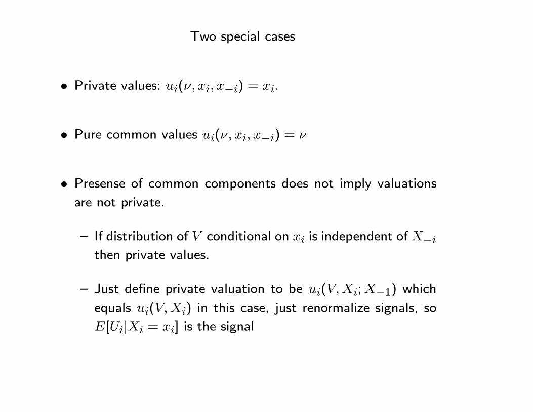
Two special cases

• Private values: ( −) = .

• Pure common values ( −) =

• Presense of common components does not imply valuationsare not private.

— If distribution of conditional on is independent of−then private values.

— Just define private valuation to be (;−1) whichequals () in this case, just renormalize signals, so

[| = ] is the signal

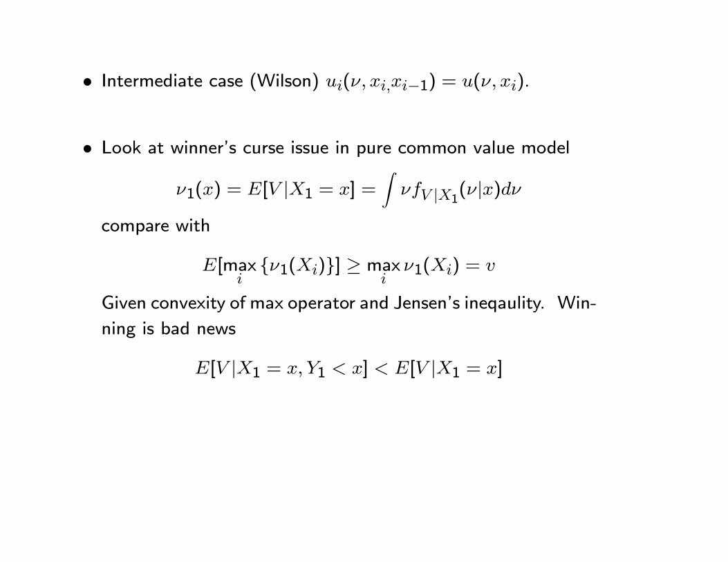
• Intermediate case (Wilson) ( −1) = ( ).

• Look at winner’s curse issue in pure common value model

1() = [ |1 = ] =Z |1(|)

compare with

[max{1()}] ≥ max

1() =

Given convexity of max operator and Jensen’s ineqaulity. Win-

ning is bad news

[ |1 = 1 ] [ |1 = ]

Section 3: Structual analysis of 2nd Price Auctions

• 2nd price are easier to model. But price also doesn’t do as

much work (no competition effect in choice of bid)

• 3.1 Theory English auction (let’s do the “button” auction)

( ) = (( )|1 = 1 = ]

• For button, bidding strategy is (using affiliation in argument)

() = [( )|1 = 1 = ] = ( )

Suppose bidding has reached = () (all else playing there),

payoff positive if and negative if .

• Reserve price

∗() = inf {|[( 1)|1 = 1 ] ≥ }

• Suppose Private values. Then equilibrim is unique (don’t

need to assume independence, very general. See Vickry).

• Common Values: not unique. Wallet game ∈ [0 ] bidfor the pot (money in both wallets, 2nd price). Equilibrium

parameterized by

1(1) = (1 + )1, 2(2) =µ1 +

1

¶2.

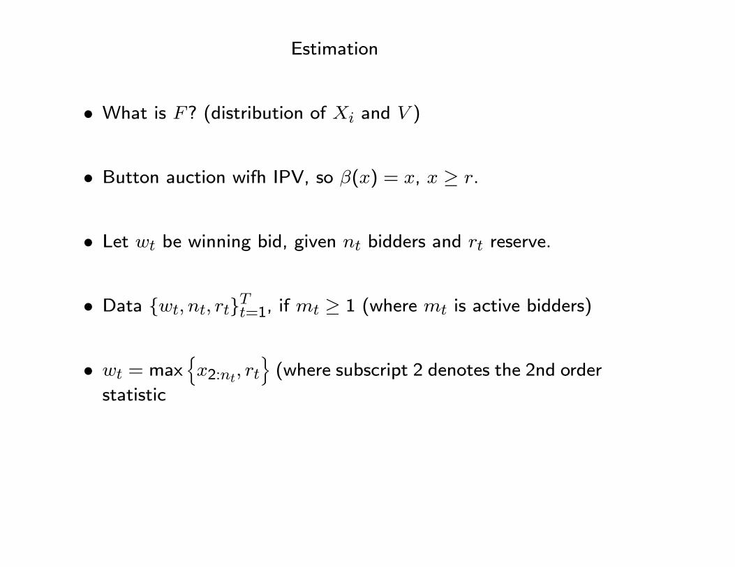
Estimation

• What is ? (distribution of and )

• Button auction wifh IPV, so () = , ≥ .

• Let be winning bid, given bidders and reserve.

• Data { }=1, if ≥ 1 (where is active bidders)

• = maxn2:

o(where subscript 2 denotes the 2nd order

statistic

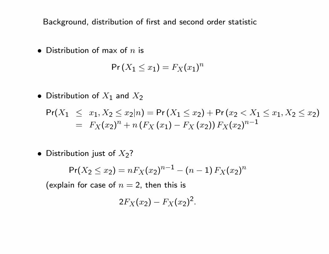
Background, distribution of first and second order statistic

• Distribution of max of is

Pr (1 ≤ 1) = (1)

• Distribution of 1 and 2

Pr(1 ≤ 1 2 ≤ 2|) = Pr (1 ≤ 2) + Pr (2 1 ≤ 12 ≤ 2)

= (2) + ( (1)− (2))(2)

−1

• Distribution just of 2?

Pr(2 ≤ 2) = (2)−1 − (− 1)(2)

(explain for case of = 2, then this is

2(2)− (2)2.

Take set where first draw less than 2 plus events where sec-

ond draw less then 2. These include all cases where second

highest is less then 2. However, there is double counting,

(events where both are less than 2 are counted twice. Then

density function for the distribution of the second order sta-

tistics is

2() = 2()− 2()()

Donald and Paarsch (1996) (Parametric approach, IPV)

• = 0, Pr( = 0) = ()

• = 1. = and Pr( = 1) = ()−1 (1− ())

• 1, then ∼ () = (1 − 1)()−2(1 −

()]() (reduces to formula above for = 2)

• Define = 1, if = 1, = 0, if 1

• Likelihood function

=Y

⎡⎣()1− Pr { = 1}

(1− Pr { = 0})

⎤⎦

• Pick to maximize given (·|). With the answer can

solve question of maximizing reserve

= 0()+()

−1 [1− ()]+Z

(−1)()−2 (1− (

with solution

= 0 +1− ()

()

which is indepdent of .

Nonparametric Approachs

• Take independent private values. Let’s take simplest case

with no reservation price. We see 2:

• What next? Athey and Haile do statistics. Not surprising

that can you back out an underlying distribution if see second

highest of draws (obviously in great shape if you see all the

bids!) Nonparametric approaches are straightforward here.

• Suppose private values by correlated. Then not in good shape.

• Suppose independent but common values. Have multiple

equilibria issue.

• What about correlation? How does this affect reservation

prices? (See Aradillas-Lopez, Gandhi, and Quint)

Symmetric First-Price Auctions (Hendricks and Porter Handbook

Chapter)

• Assume bidders, using a common bid function with inverse. Then bidder 1’s profits from bidding given a signal are

( ) =Z ()

[( )− ]1|1(|)

Differentiating w.r.t.

[( ())− ]1|1(()|)

−Z ()

1|1(|) = 0

and imposing symmetry and = () and = 1

0() yields

[( )− ()]1|1(|)

− 0()1|1(|) = 0

The equilibrium bid solves this differential equation, subject to

the boundary condition (∗) = (where ∗() is the lowest

signal such that the expected value conditional on winning isat least the reserve price. The solution is

() = (∗|) +Z

∗( )(|)

where

(|) = exp

⎧⎨⎩−Z

1|1(|)1|1(|)

⎫⎬⎭• The symmetric equilibruim exists under fairly weak regularityconditions on . (Assumption of a binding reserve priceensure that there is a unique symmetric equilibrium

• Special case of affiliated private values, the equilibrium bidfunction reduces to

() = −R 1|1(|)1|1(|)

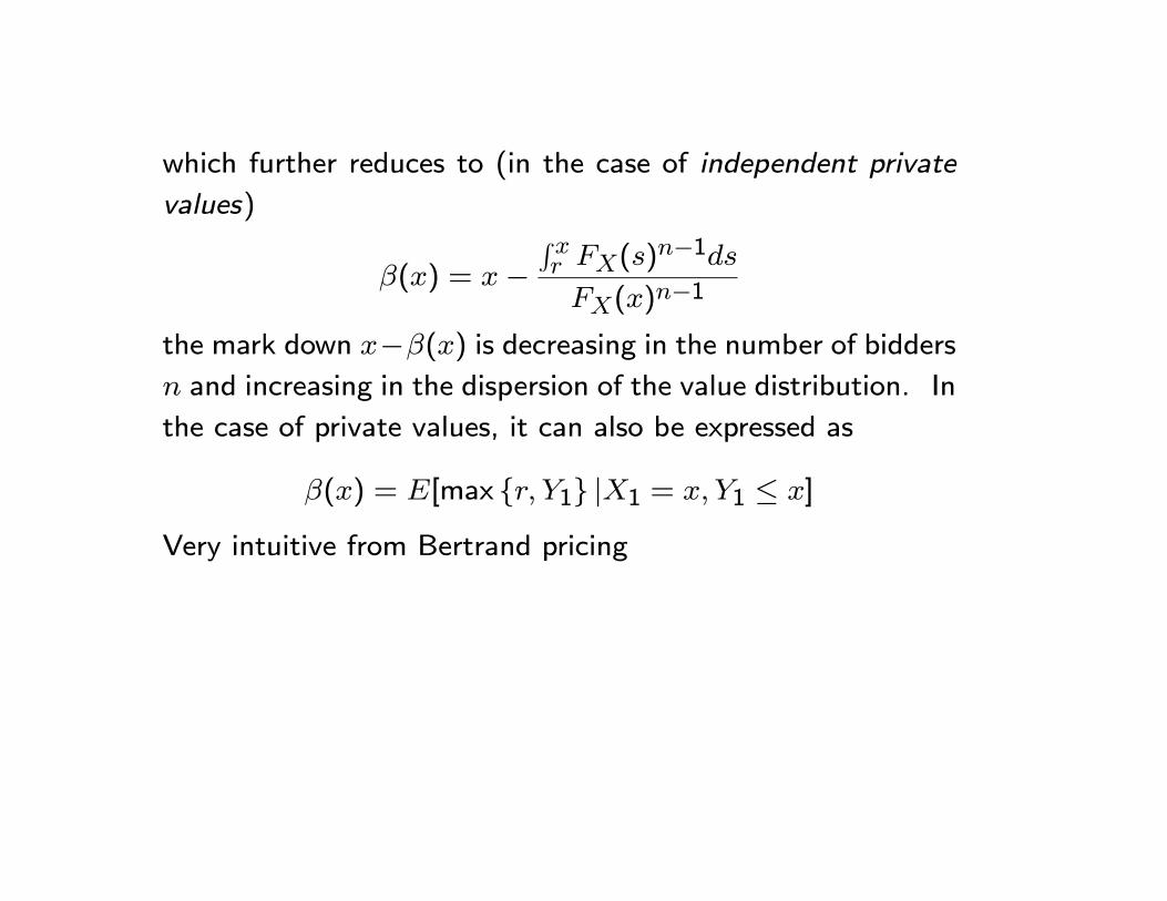
which further reduces to (in the case of independent private

values)

() = −R ()

−1()−1

the mark down −() is decreasing in the number of bidders and increasing in the dispersion of the value distribution. In

the case of private values, it can also be expressed as

() = [max { 1} |1 = 1 ≤ ]

Very intuitive from Bertrand pricing

Estimation

• Discuss MLE approach of Paarsch. Winning bid is observedif and only if 1: ≥ . Probability of no one winning is

(). The probability distribution function of is

() = (())−1(())

0() =

(())

( − 1) (()− )

• Can construct a likelihood function. (Then after estimation

can calculate optimal reserve price, for example

Nonparametric Approach (Elyakime, Laffont, Loisel, Vuong

(1994)+Gueere, Perrigne, and Vuong (2000))

• Data on bidsn{}

=1 o=1

• Recall in symmetric equilibrium

(()− )1|1(()|()0()− 1|1(() ()) = 0

• Define 1 = (1) as the maximum bid of bidder 1’s rivals

and let conditional distribution of 1 given bidder 1’s bid

1 be denoted 1|1(·|·) and density given by 1|1(·|·).Montonicity of and implies that for any ∈ ( ()),

1|1(|) = 1|1(()|())

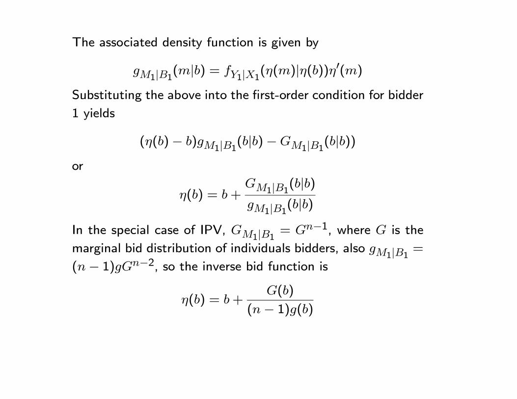
The associated density function is given by

1|1(|) = 1|1(()|())0()

Substituting the above into the first-order condition for bidder

1 yields

(()− )1|1(|)−1|1(|))

or

() = +1|1(|)1|1(|)

In the special case of IPV, 1|1 = −1, where is the

marginal bid distribution of individuals bidders, also 1|1 =(− 1)−2, so the inverse bid function is

() = +()

(− 1)()

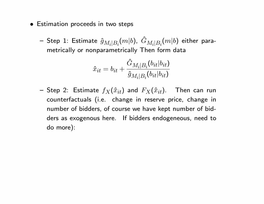
• Estimation proceeds in two steps

— Step 1: Estimate |(|), |

(|) either para-metrically or nonparametrically Then form data

= +|

(|)|

(|)

— Step 2: Estimate () and (). Then can run

counterfactuals (i.e. change in reserve price, change in

number of bidders, of course we have kept number of bid-

ders as exogenous here. If bidders endogeneous, need to

do more):

Putting these ideas to work. Hortacsu and Kastl

• Study auction of 3month and 12 month treasury bill in Canada

• Dealers submit bids for themselves, as well as customers. Sosee what customers do. What do dealers get out of the

additional information (what is value)

— And what is this info? Fundamental value, or info about

competition?

• Start with a null hypothesis of private value (so not learningabout fundamental value)

— Create a test statistic and can’t reject private values

— Then estimate the value of the information about the com-

petition

Data

• Who are these dealers and customers?

— Desjardin Securities, JPMorgan not dealers, but customers

— BNP Paribas and Bank of America are ”customers”...

— Major thing left unexplained is why we have customers

”customers are typically large banks that for some reason

choose not to be registered as dealers.”

— Look at summary statistics. Look at # of customers,

pretty small. Would have expected the dealers to be small

in comparison to number of customers.

Preliminary Evidence

• 3M sample, out of 660 dealer bids also accompanied withcustomer bid, 216 previously placed dealer bids were updated.

• 12M sample, 275 out of 659 are updated.

• Info that bids are correlated with updated bids. (But wouldhave been nice to see the correlation with updated bids fromother customers that they don’t see)

• What about cases where not updated? Argue there isn’tmuch time left. Takes about 5 minutes to put a new bidin and when customer submits bid with less then 5 minutesto go, can’t react. (Could use as a benchmark reactions tocustomer bids from dealers.)

Model of Bidding

• Two classes of bidders, number of potential dealers,

number of potential customers

• Discriminatory auction (pay as bid)

• Bid for shares of which is random

• Before bidding, players observe private signals 1 2 1

.

• Stage 1 of bidding: dealers may submit 1(|), specifies foreach price how big a share of the securities dealer demands

given signal (Assume constrained to use step function, with

finite steps)

• Stage 2: customers get matched to a dealer, bid (|)

• In stage 3, dealers may submit a late bid, 3( ),

where contains all new information (including bid and any-

thing else)

• Rationalize early bidding, assume some probability won’t beable to make a second bid, so put something in. Has some

complicated stuff about observing a signal about whether the

dealer will or will not have a chance to submit late bid...

• Assumption 1: 1 2 1

., independent and drawn

from common support (symmetric private values), c.d.f. ()

and ()

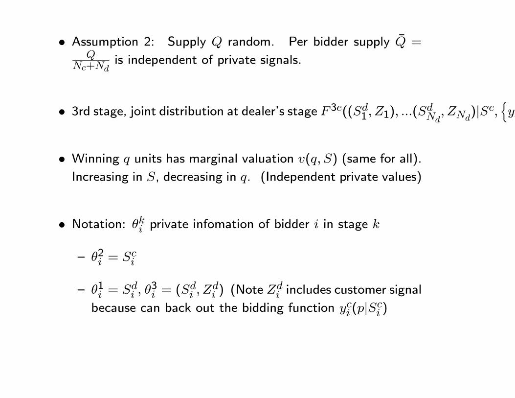
• Assumption 2: Supply random. Per bidder supply =

+is independent of private signals

• 3rd stage, joint distribution at dealer’s stage 3((1 1) (

)|n

• Winning units has marginal valuation ( ) (same for all).Increasing in , decreasing in . (Independent private values)

• Notation: private infomation of bidder in stage

— 2 =

— 1 = 3 = (

) (Note

includes customer signal

because can back out the bidding function (| )

• Equations 1 and 2

— Dealer at stage 1

Pr( ≥ |) =

⎛⎜⎝− X∈

(|)−X

∈\(| ) ≥ 1(|)

⎞⎠

— Dealer at stage 3

Pr( ≥ | ) =

⎛⎜⎝− X∈\

(|)−X

∈\(| ) ≥ 3(

• Proposition 1 (Kastl (2011). If no learning about fundamen-tals (includes IPV case), bid functions satisfy

( ) = +Pr(+1 ≥ |)

Pr( +1|)( − +1)

• Discussion of result. Write equation as (pretty intuitive)

(( )− ) Pr( +1|) = Pr(+1 ≥ |)(−+1)

This is the FONC of changing cutoff quantity . One issue

is it seems firms leave this cutoff the same, vary bid. Not a

FONC for fixed cutoff, varying bid.

Estimating marginal distributions

• Start with discussion of previous literature (Hortascu and McAdams,Kastl) where symmetric (no dealers)

— if bidders are ex-ante symmetric, private information is

independent across bidders and data generated by a sym-

metric Bayesian Nash equailibrium.

— Fix bidder. Draw randomly − 1 actual bid functionssubmitted by bidders.

— Simulates one state of the world, so one potential realiza-

tion of residual supply

— Given bid, and residual supply can obtain a market clearing

price. Get a full distribution of market clearing price given

a fixed bid. For a given bid (step function) we can use

the distribution of the market price and

( ) = +Pr(+1 ≥ |)

Pr( +1|)( − +1)

to back out marginal value at each step.

• Now two classes of bidders. Dealer bidding at stage 1

— Draw customer bid (equals zero means non-participation)

— If no customer, draw from pool of dealer bids with no

customer participation

— If have customer, draw from pool of dealer bids with a

similar customer (why not just give the dealer that went

with the customer?)

• To estimate the probability for state 3, draw − 1 bids andtake obseved customer bid to plug in.

Value of Information

• Π3( ) expected profit stage 3, including info from cus-

tomer

• Π1(). before arrive.

=Z ∞0

Π3( )( 3( ))−

Z ∞0

Π1()( 1())

• For stage 3 case, see one customer, integrate out the others,for stage 1 case integrate out all customers.

• Note, cannot calculate value of the system through this exer-

cise (i.e., what happens if stage 3 bids are banned)

• Estimate the = 45 basis point. (64 when use 4 auc-

tions, 46 when 2, 26 when 1). (1.35 million per dealer per

year)

• Compare to average expected profit of 1.65 basis points.