attitudes toward risk: theoretical implications of an ... economic journal, 9i (december i98i),...
TRANSCRIPT

Attitudes Toward Risk: Theoretical Implications of an Experiment in Rural IndiaAuthor(s): Hans P. BinswangerSource: The Economic Journal, Vol. 91, No. 364 (Dec., 1981), pp. 867-890Published by: Blackwell Publishing for the Royal Economic SocietyStable URL: http://www.jstor.org/stable/2232497Accessed: 13/10/2008 14:55
Your use of the JSTOR archive indicates your acceptance of JSTOR's Terms and Conditions of Use, available athttp://www.jstor.org/page/info/about/policies/terms.jsp. JSTOR's Terms and Conditions of Use provides, in part, that unlessyou have obtained prior permission, you may not download an entire issue of a journal or multiple copies of articles, and youmay use content in the JSTOR archive only for your personal, non-commercial use.
Please contact the publisher regarding any further use of this work. Publisher contact information may be obtained athttp://www.jstor.org/action/showPublisher?publisherCode=black.
Each copy of any part of a JSTOR transmission must contain the same copyright notice that appears on the screen or printedpage of such transmission.
JSTOR is a not-for-profit organization founded in 1995 to build trusted digital archives for scholarship. We work with thescholarly community to preserve their work and the materials they rely upon, and to build a common research platform thatpromotes the discovery and use of these resources. For more information about JSTOR, please contact [email protected].
Royal Economic Society and Blackwell Publishing are collaborating with JSTOR to digitize, preserve andextend access to The Economic Journal.
http://www.jstor.org

The Economic Journal, 9I (December I98I), 867-890
Printed in Great Britain
ATTITUDES TOWARD RISK:
THEORETICAL IMPLICATIONS OF AN
EXPERIMENT IN RURAL INDIA*
Hans P. Binswanger
In economics, empirical work with models of behaviour under risk - whether security based or utility based - usually involves comparing the models' predictions with the real world decisions of a sample of individuals or firms (for utility-based examples in agriculture, see Anderson et al., I977, or Halter and Dean, I97I; for a safety-based example, see Roumassett, I973). The advantage of this approach is that the analysis focuses on decisions that people actually must make in the course of their economic activities. The disadvantage is that it is difficult to determine the relative influence of risk and other factors on these decisions. This difficulty has led experimental psychologists and, to a much lesser extent, economists to design specific experiments to test the implications of utility theories in the laboratory. (For reviews of this experimental work, most of which has been confined to utility-based theories, see Luce and Suppes, I965, and Grether, I978.)
This paper, following the lead of the experimental psychology literature, discusses a relatively simple but fairly large-scale experiment in rural- India that the writer and colleagues at ICRISAT designed to measure attitudes toward risk. We chose an experimental approach when it became clear that we could not obtain reliable estimates of risk aversion by the usual interview techniques of eliciting certainty equivalents. (For details of the difficulties encountered in this study and a description of the entire experiment see Binswanger, I980.)
We have validated our experimental measures of risk aversion by showing that a portion of the observed variation among individual farmers' agricultural decisions can be related in a systematic manner to variations in the same far- mer's experimentally measured degrees of risk aversion, the more risk averse choosing more conservative options (Binswanger et al. i980).1 This observed relationship between experimental behaviour and actual farm decisions sug- gests the importance of examining the significance of our findings for a number of models of behaviour under risk, focusing on the consistency of our findings
* The experiment on which this paper is based was carried out as part of a wider research programme of the International Crops Research Institute for the Semi-Arid Tropics (ICRISAT) on the role of risk in agriculture and with ICRISAT's generous support. The author would like to thank B. C. Barah, R. D. Ghodake, S. S. Badhe, M. J. Bhende, V. Bhaskar Rao, T. Balaramaiah, N. B. Dudhane, Rekha Gaiki, K. G. Kshirsagar, Madhu Nath and Usha Rani who helped in carrying out the experiment. Comments by Harvey Lapan and one anonymous referee were particularly helpful in preparing this paper. Extremely detailed and helpful comments were made by Mark Machina who was the reviewer for this JOURNAL. Of course, responsibility for any remaining errors rests with the author alone. Vir- ginia Locke's editing greatly-added to the clarity of the paper. The views expressed in this paper do not reflect those of the World Bank or of ICRISAT.
1 The agricultural decisions examined were those related to sowing time, fertiliser use, initial fertiliser adoption, fallowing behaviour, and irrigation investment.
[ 867 ]

868 THE ECONOMIC JOURNAL [DECEMBER
with a varied set of theoretical predictions. Many decision rules are considered, and a number of different approaches are used to predict how the respond- ents should have behaved in the experiments if they had used a particular rule.
In the first section we review the experimental method and the key results. In the second major section, we turn to utility-based models. The nature of the experiment discussed here restricts tests of the utility-based models to questions concerning the shape and intertemporal stability of the utility function. Thus we will look at the way various measures of risk aversion behave as wealth and gain levels change. We will examine an empirical test of the asset integration hypothesis, by which that hypothesis is rejected. For a discussion of the asset integration hypothesis, see Kahneman and Tversky (I979).
Safety-based models of behaviour are considered in the third section of the paper. It is shown that predicting behaviour with these supposedly simple rules is often not straightforward. Furthermore, the predictions derived with these models are seen to be inconsistent with the experimental behaviour re- ported. The final section of the paper provides a discussion of the study's results.
I. THE EXPERIMENT AND THE KEY RESULTS
The experiment makes no theoretical restrictions; individuals choose among alternatives in which an increase in expected returns can be purchased only by increasing risk or the dispersion of outcomes. Unlike most of the studies to date in psychology and economics, this experiment used pay-offs that were both real and large to induce participants to reveal their preferences. Indeed, the highest expected payoff for a single decision exceeded the average monthly income of an unskilled worker.
The subjects of the study were 330 individuals selected at random from six villages of the semi-arid tracts of Maharashtra and Andhra Pradesh.' The experiment itself consisted of a sequence of games, with real and high pay-offs, that were played in the following way: People were offered a set of eight choice alternatives in which high expected returns could be purchased only for a large standard deviation. Alternatives A to F are described in the top panel of Table I. Each consists of a 'good luck' and a 'bad luck' outcome and its probability, of 1/2, is decided on the toss of a coin. Alternative 0 provides a fixed and certain outcome: The individual is simply paid Rs. 50. Alternative F pays nothing or Rs. 200 with equal probability. A risk averse individual would prefer alterna- tives B to B*, C to C*, and E to F, since each pair of alternatives has the same expected value but B*, C*, and F each have higher spreads than B, C, and E, respectively. (The moves from B to B*, C to C*, and E to F are therefore what Rothschild and Stiglitz (1970), have called mean-preserving spreads.) Only the alternatives shown in Table I were available for choice. Each alternative was
1 The sample was taken from a rural population in which agriculture or agricultural labour is the primary or secondary occupation. By international standards most households in the sample are poor, but they vary greatly in terms of wealth and other personal characteristics. The mean physical wealth of the sample was Rs. 27,600 in x978/79, with a coefficient of variation (c.v.) of I 36 %; mean years of schooling was 26, with a c.v. of I30%. Mean age of the sample was 42 years, with a c.v. of 30%.

198I] AN EXPERIMENT IN RURAL INDIA 869
labelled (column heads in Table I) to indicate the degree or risk aversion its choice by a subject represented. These labels were arbitrary and were not re- vealed to the respondents. More precise measures of risk aversion are discussed later.
The game was played - and pay-offs were actually made - seven or eight times over a period of six weeks or more, and between one day's and two weeks' time was allowed between games for reflection. Respondents did not know in advance how many times the games would be played or at what level. In the first 5 games all amounts shown in Panel I of Table I were divided by IOO; that is, alternative F paid Rs. 2 on good luck, whereas alternative 0 paid Rs. 0.50 consistently. This set of 5 games was called the Rs. o.5o game level. At least two weeks later two games were played at the Rs. 5 level (all amounts in panel I divided by I o). After two more weeks a subsample of I I8 household heads played the Rs. 50 game and it is only the results for this subsample that are shown in panel II (see Table I, footnote t on sample size variations). Chi-square tests showed that at the Rs. 5 level the risk-aversion distribution of the subsample whose results are discussed here could not be distinguished statistically from the risk-aversion distribution of the other household heads or of the latter's wives, who did not play the Rs. 50 game. Finally, two weeks after the Rs. 50 game, respondents were asked hypothetical questions about how they would behave at the Rs. 500 level. Although we show the results for this hypothetical question, we do not use the answers at that level of payoff in the tests performed in this paper.'
The results in panel II show that, when payoffs are small (Rs. o.so), we find nearly 50 % of respondents in the intermediate and moderate risk-aversion categories (B and C). Over a third of respondents show a nearly neutral or risk-preferring behaviour pattern (E or F), and less than I0% are extremely or severely risk averse (O or A). When game levels rise, the proportion of indi- viduals concentrated in the intermediate and moderate categories rises until it reaches 8o % of all the respondents in the panel. Near neutral and risk- preferring behaviour virtually disappear: only one out of I I 8 individuals choose F. On the other hand, the proportion of extreme and severely risk-averse choices stays below I0 % up to the Rs. 50 level and rises to I6 % at the Rs. 500 level. The extremely risk-averse fraction never exceeds 2-5 %. Thus at higher game levels, the risk aversion distribution is single peaked, concentrating mostly in the two intermediate and moderate risk aversion classes B and C.
II. IMPLICATIONS FOR UTILITY FUNCTIONS
Utility-based models of behaviour under uncertainty have been developed by statisticians, economists, and mathematical psychologists, and a very careful review of these models was offered in the mid- I 960s by Luce and Suppes (i 965) .
1 The usefulness of hypothetical questions, both outside and within this game context, is discussed extensively in Binswanger (I980). It appears that toward the end of a prolonged game sequence, individuals do reveal preferences in hypothetical games that are consistent with their actual game behaviour.

870 $0 IC$
> V -4 04
4
&4 0 -t,41 t '.. to C4 LO 4-J C,
rA v
0 Lo M 114 14
C4 0 >1 Cd 04
'o 0 0 -4 C,3 j cd o r4 4 u
0 0 0 W2v
O --4 IC4. 4)
cl > %) ++ eQ.
Cd b-0 4) w 5
4-J
0 s-4 +j cl
Cd 0 Cd m r-- 00 co COD C b4 0-4 6-4 04
v cd 1.
'>
z 0 > -4 4-)
C13 4) Cd P
Cld $4 > t v Cd su-4 C's
141:1 4-J 0-
0 0 Cd t.4 -14
0 V o u u cd cd
> 0-4 4 4j 0 ..4 co
4 4-
u cq 04 0 e4
0 u cd Cd ITZI C's co L)
4
&4 to-4 LO t.2 0 o >
Cd ce) V 4 4-J -4
0-4 4) rA Cl -.4 0
4 Z .54 94 Z Cd 04 0u u 4 -4
$4 &4 4-i 4-J rA C,
0 $-, Le) Lo 4-i '12
0 0 0 0 0 0 0 > Cb Cb b w ,o v C. 9 -0 bo
4) cl 6-4 W w w 0 w V/ 0 = &4
0 v Cd 0 Cl g4 0 :3 biD 4
Cd oj 4 04 V 14 -4 ICA, Cd > : 0'bo cd >
di 1.44 0 -4
00 O w > co .104
1-4 Cd Cd 0 1-4
0 co 0 '41' 0-4 0 -.4 IL)
0-4 0-4 O
rA 0 4-J -4
biD Z ;zj 0 0 tb 6 +- , 0 O -14
LO &4 OC) 0 1-4 &
ts Cd --4 0
> 0 ...4 41
0 0 -1-4 Cd 0 O 0-4
rA
Cd 4 r,44 $-4 >1 0 bJD
Lo cl 0 4 t'. Cd Cd 4) V 04 ..4 .
'A LO "d' 0 0'- 4-J 'O U)
Cd -.A 8 V., LO NO m $-4 C13 C) - C4 00 00 00 rA IR14 o 4i 4-1 $-4 0 0 'Z Lo 0 rA
cel) LO 10 ar) Cb ICI n Gn 0 V 4 C's cl Cld 1-4
C4 ce) Ce) Ci 0 8 u -4 0 4-h 4 4-) 44 bO
Cd rA 4
Cd 0 4 4 944
04 $-4 0 4.)
4)0 4
94
Cd rA 0 -142
4 cn J u +, t) C4-4
4 4 i 0 50 >
cl 4 >v )--4 (M 0 O cl -t: -0 Lo to oo t- 00 0-4 00 0
o O a , )..q 71
. 1, -'A ( bJO 0-4 8 00 'A cb ;I C;Z.. C. cis
0-4 04 0 04
ci 04 er) LO 4-1 > - +4
4 0 44 0
Cd 0
4 4-J -4 -1-4>
Cd0 >
04
Cd OJ -4J
Q
-4 > v
co > O cd 4
00 "44 --, C) -4 LO
O cd 0
C) Lo o Id4 o co 1,4Q 0 $14
LO LO c c 0
.1 t"o Cd $-4 t-W4 Cb 60 (4 114 00
4.) Cd 44 C,$
g4 0 0 >S 4 U) 44 Cld r. t.0 Cd -4
0 0 0
> 4
0
C-d t! Cd cdv
LO 0 > 0 0
LO Lo 1-4 LO 40 -14 0 cl
0 0 M LO LO Lo 4
9 . rll-. v;, L: 4 .O. 0 LO to A 0 0 LO LO
(:;4
>
4-J A A A 0-4 1-4 -.4 -14 0
Q0 t.O W A A Z
.44 $4
Cd 0 b > tn Cd -4>.4., V V
C3 $14 Cd Cd> 4-1
C d P4 .4>
4 Cd cl
$4 a
Cq Cdv cd P4
1-4 4-J bt) 0-
Cd g4 4 $0
cd cd 4.,
P4 0 $- 1-4
-4 0 0 b 44 n- t-;4'
o 0 cl
to 4-J
0-4
441)
C"
C'
C) LO 6 >
LO cd0 0
4) -4 74) "Z, 0 0
0 gi I.-I ;> cd Cd 1 4 0 0 4.1 0, :3 0 0 C) -4 r4O &
-4 to 0 g Cd
41 4--Jt 6, 0 O >
LI? O O LI? O 0 -4 IS 4.)
to LO LO 0 LO LO 0 LO cn W Cd 0
44-5) $-4 -4 s., -40O-)
:z ++ Cd 0 --q :3 Wt.0
cl m 0 CIS W ;I 0.4>

I98I] AN EXPERIMENT IN RURAL INDIA 87I
With the exception of Kahneman and Tversky's (I979) prospect theory, few theoretical proposals have been made since that review.'
The basic purpose of all utility models is to associate with each action or prospect aj a unique utility value U. such that a decision maker will choose a, over a2 (a1 > a2) if, and only if, the utility value of a, exceeds the utility value of a2 or is equal to it,2 that is
a, > a2 U(al) _ U(a2), (I)
where > indicates a relationship of preference or indifference. The outcome of each action depends on which event Ei will occur. In all formulations, the decision maker is assumed to associate objective probabilities or subjective probabilities (or decision weights) with each event Ei. Furthermore, the action aj associates an outcome (usually money income or wealth) with each event Ei.
For simplicity, the discussion that follows will be restricted to discrete proba- bility distributions. All the theories share the utility function structure,
Uj = 2riU(Xii), (2) i
where rri is a 'probability' measure in either an objective or subjective sense. Note that in this formulation utility and probability combine multiplicatively for each individual event and that these products are summed over the set of events. Tversky (I967) has tested this basic formulation experimentally for a large class of more specific models that can be derived from equation (2) and has found his experimental results to be consistent with additivity of the utility contributions of each possible event.
In the expected income (EI) model the utility function is linear, and objective probabilities Pi are used as decision weights, that is, U, = YiPiXi. In the expected utility (EU) model, for which Von Neumann and Morgenstern (I947)
provided underlying axioms, a utility function, which is typically assumed to be concave, is used to weight outcomes, that is, U2 = Y2P1 U(X1).
In the subjective expected utility (SEU) model associated with Ramsey (I93I)
and Savage (I954), objective probabilities are replaced by subjective proba- bilities HIj to form the utility index U3 = Ei HI U(Xi). This is the model preferred by economists. The mathematical psychology literature has attempted to make subjective probabilities a direct and, as the authors hope, unique function of objective probabilities by writing HIj = h(Pi).
The subjective expected income (SEI) model (used first by Preston and Baratta (I948) in an attempt to measure probability preference functions h (Pi)) assumes that the utility function has the form U4 = Zih(Pi)Xi, that is, that it is linear in the outcomes. This theory has recently been revived by Handa (I 977), under the name of certainty equivalent approach, in an attempt to provide it with an axiomatic underpinning (see, however, Fishburn's, I978, objection).
Most psychologists work with subjective expected utility models very close
1 A more recent review of the models can be found in Binswanger (I 978) . In the present paper, only issues that have been examined experimentally are discussed.
2 Probabilistic models deal with deterministic choice over randomly fluctuating utility functions or with probabilistic choice over a stable utility function. However, these models are not relevant here.

872 THE ECONOMIC JOURNAL [DECEMBER
to the SEU approach just described, except that they assume a more or less stable probability preference function and write U5 = Zih(Pi) U(Xi); that is, they weigh both probabilities and outcomes' and work with utility functions in gains and losses rather than in final wealth states. Kahneman and Tversky (I979) have extended this approach under their prospect theory.
Because they consist of two-outcome gambles with equal probabilities, the experiments on which this paper is based cannot address the issue of probability preferences. However, this feature of the experiments is precisely what allows us to test some curvature properties of the utility function as if probability preferences were not present.
The experimental evidence of Table i clearly indicates that, at high levels of income, virtually all individuals are risk averse; we can therefore reject the expected income and the subjective expected income (certainty equivalent) approaches to utility indexes.2
Measures of Risk Aversion Let W stand for final wealth and consist of initial wealth w) and the certainty equivalent of a new prospect M, that is, define
W= w)+M. (3)
On a utility function U(W) = U() + M), we can define risk aversion in several ways. For example, let subscripts to U denote the respective derivatives, that is, Uw = 9U/IW, etc., Pratt has defined:
absolute risk aversion Q = - uww UM= uj (4)
relative risk aversion R = - W w = WQ. (5) UW
When we evaluate R at the point (w + M) this becomes
R = (w+M)Q. (6)
Furthermore, both Menzes and Hanson (I970), as well as Zeckhauser and Keeler (I970), have defined the following measure:
S=-M UWW=MQ. (7)
1 This is not the place to discuss the probability preference literature, but attempts to measure such preferences practically stopped after it proved difficult to find stable functions. Such measurements have been attempted by Preston and Baratta (I948), Griffith (I964), Sprowls (1953), Edwards (I953, 1954) and others. Theoretical problems associated with stable functions were first noted by Edwards (I955), who as a consequence developed the non-additive subjective expected utility (NASEU) model.
2 The subjective expected income approach is in fact rejected by a direct contradiction of one of its basic axioms which Handa (1977) postulated. This axiom (called enhanced prospects by Handa) says that the ranking of bets should be unaffected by the multiplicative transformation of all of their outcomes by the same constant that is used in the experiment discussed here. In a sense it does not rule out risk aversion, but it does assume what amounts to constant partial risk aversion. Handa is uneasy about this assumption but defends it by saying that it may hold for games in the neighbourhood of normal business transactions. But normal business transactions of the households considered clearly include all payoff sizes from thc 0o50 to the 5oo rupees game. And the ordering of prospects changes for most individuals within that range.

I98I1 AN EXPERIMENT IN RURAL INDIA 873
Menzes and Hanson used the term partial relative risk aversion for 8, which we will abbreviate as partial risk aversion. (Zeckhauser and Keeler used the term size-of-risk aversion.)
Partial risk aversion is equal to relative risk aversion for individuals with zero wealth. As shown by several authors, it follows from the preceding equa- tions that the three measures are related to each other as follows at the point
R = OQ+S. (8)
In fact, once Q, o and M are known, all three can be computed. Since Q can be computed both from a utility function in terms of net gains and from one in terms of wealth, it does not matter for measurement purposes with which speci- fication one starts.
The three measures have the following interpretation. Consider the prospect (X, P) where X and P are vectors. Note that prospects here are defined in terms of gains and losses from whatever initial wealth may happen to be. Absolute risk aversion traces the behaviour of individuals to the prospect (X, P), as their wealth rises and the prospect remains the same. We usually assume decreasing absolute risk aversion, which implies that an individual's willingness to accept a given fair gamble should rise as wealth rises.
Relative risk aversion traces the behaviour of an individual as both wealth and the size of the prospect (X, P) rise. Let k be a scalar. Consider the individual in a new position in which he or she now owns wealth kW and is confronted with the prospect (kX, P). Arrow (I 97 I) hypothesised increasing relative risk aversion, which implies that an individual's willingness to accept a given gamble de- creases when both wealth and all outcomes of a gamble are multiplied by the same constant.
Partial risk aversion traces the behaviour of an individual when the scale of the prospect changes by a factor k but wealth remains the same. Increasing partial risk aversion implies a decrease in the willingness of the individual to take a gamble as the scale of the prospect increases.
Menezes and Hanson have also shown (for an individual who has nonzero wealth and who is risk averse) that if partial risk aversion is monotonic in k, then it must be constant or increasing with an increase in prospect size k. Note that in the experiment under discussion, prospect size was varied by a factor of ioo but wealth was left virtually constant.' Menezes and Hanson would therefore predict a leftward shift of the distribution of risk aversion as game scale rises. This result is confirmed in Table I and is statistically significant.
To measure risk aversion coefficients, therefore, one should use a utility function that exhibits increasing partial risk aversion (IPRA). Such a function is discussed in Binswanger (I978) and Sillers (I980). However, the function has the disadvantage that its parameters must be estimated from the observed choices that an individual has made at two game levels. Thus for each individual
1 Since modal wealth is about Rs. 13,000, the payoffs of Rs. 40 that were typically received prior to the Rs. 50 game 'multiplied' wealth by a fraction k of I-004. This fraction is negligible relative to the k of I00 that obtained between the Rs. 0-5o and Rs. 50 games.

874 THE ECONOMIC JOURNAL [DECEMBER
we would have to approximate the risk aversion associated with a game at a given level separately, depending on the individual's choices. To simplify matters and obtain a unique risk aversion coefficient for each game level, we used a constant partial -risk aversion- (CPRA) function as an approximation [U = (I- S) M1-s]. Fortunately, the approximation of S, using CPRA, to risk aversion coefficients computed for various choice paths using the IPRA function was very close.' For details of the computations of the values in panels IV and V of Table I, see footnote t to that table. A full discussion of all scaling issues involved is offered in Binswanger (I980).
Panels IV and V of Table I illustrate the behaviour of the absolute and rela- tive risk aversion coefficients. The number assigned to each alternative at each game level is a separate local approximation under the assumption of a utility function with constant partial risk aversion in the neighbourhood of the payoff levels involved in the alternative. The numbers in panel IV and V have to be viewed in conjunction with the frequency distribution of the choices in Table i and with the geometric means of absolute risk aversion that were computed from the distribution of choices. These geometric means (see right-hand side of panel IV, Table I) indicate that on average, absolute risk aversion is indeed declining as payoff increases.2 This result is consistent with the notion that individuals' willingness to engage in small bets of fixed size should increase as their wealth rises (Arrow, I 97 I) .
On the other hand, contrary to Arrow's (I97I) prediction, relative risk aver- sion is also declining. The numbers computed in panel V refer to an individual with a wealth of Rs. Io,ooo, somewhat less than the modal wealth. However, for wealth levels in excess of Rs. Io,ooo the qualitative conclusion discussed below holds: With the exception of overall risk neutrality - that is, of a choice pattern of alternative E or F at all game levels - relative risk aversion of the sample households must be declining. In particular, for the 'average' choice pattern the following is the case. At the Rs. 0o50 level the average absolute risk aversion coefficient places the centre of the distribution between choices C and E. The centre shifts to choice B at the Rs. 500 level. Thus on average, rela- tive risk aversion declines from an order of 03 to an order of o-oooi.
Arrow's prediction of rising relative risk aversion arises out of the following assumptions: If the utility function is bounded from below as wealth approaches zero, R cannot approach a limit above one as wealth tends to zero. On the other hand, if the utility function is bounded from above, R cannot approach a limit below one as wealth approaches infinity. Therefore, if one makes the further
1 For indifference points AB, BC CE the differences in S were less than 2 %, using the two functions. For the indifference point OA the differences were up to I 5 % but even that percentage would not affect the qualitative results reported below, particularly because so few individuals choose alternative 0, and regression results were quite stable relative to functional transformation of risk aversion measures. For details, see Binswanger (1978) or Sillers (I980).
2 Equation (7) implies that on a constant partial risk aversion function (S/aM = o) absolute risk aversion must be declining for positive M. However, we use the CPRA function only to get a local approximation of S for each alternative at each game level, and as the footnote above implies, these approximations are close. The conclusion, on the other hand, is derived from the behaviour of the geo- metric average of these approximate levels across game scales and is not sensitive to the minor approxi- mation errors involved.

I98I] AN EXPERIMENT IN RURAL INDIA 875
assumption that the behaviour of R as a function of wealth is monotonic, it must rise over the entire-interval (Arrow I97I, pp. 97, 98). However, in the experi- mental results we find that at game levels (not wealth levels) close to zero most individuals exhibit extraordinarily high levels of R.
The Concept of Asset Integration and Measures of Risk Aversion In using the concept of utility function, economists have usually chosen to express utility as a function of wealth W, that is,
U = U(W)= U(cO +M). (9)
They have implicitely postulated what Kahneman and Tversky (I979) call asset integration: The action or prospect (X, P) is acceptable at asset position W if and only if U(W+X, P) > U(W), where X and P are vectors of outcomes and of their corresponding probabilities. The decision maker is assumed to make his decisions in terms of final wealth states and not in terms of gains and losses. (Asset integration is the same as income integration, which is discussed in the next section of this paper, when total income is measured as the rate of return to the individual's endowments.)
U(W V(M)
B/
M Certain net gain
W= w +M Wealth
Fig. i. Markowitz-type utility function.
Most economists who have tried to measure utility functions empirically, however, have chosen to use functional representations of a utility function that will be stable over time in terms of gains and losses (see, for example, Halter and Dean, I97I, or Anderson et al. I977). In addition, Markowitz (I952) has proposed a utility function that has alternating concave and convex segments and is time stable in terms of gains and losses. He was prompted to propose this form of the function when he tried to find a utility function that would have some of the properties of the one proposed by Friedman and Savage (I 948) but that would avoid some of the apparent inconsistencies with observed gambling and insurance behaviour that the latter function encount- ered. Friedman and Savage assumed that their function was time stable in terms of wealth (or annualised total income). Markowitz proposed that gains
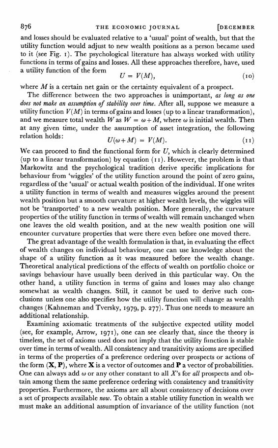
876 THE ECONOMIC JOURNAL [DECEMBER
and losses should be evaluated relative to a 'usual' point of wealth, but that the utility function would adjust to new wealth positions as a person became used to it (see Fig. i). The psychological literature has always worked with utility functions in terms of gains and losses. All these approaches therefore, have, used a utility function of the form
U = V(M), ( IO)
where M is a certain net gain or the certainty equivalent of a prospect. The difference between the two approaches is unimportant, as long as one
does not make an assumption of stability over time. After all, suppose we measure a utility function V(M) in terms of gains and losses (up to a linear transformation), and we measure total wealth W as W = co + M, where co is initial wealth. Then at any given time, under the assumption of asset integration, the following relation holds: U(w + M) = V(M). (I I)
We can proceed to find the functional form for U, which is clearly determined (up to a linear transformation) by equation (i i). However, the problem is that Markowitz and the psychological tradition derive specific implications for behaviour from 'wiggles' of the utility function around the point of zero gains, regardless of the 'usual' or actual wealth position of the individual. If one writes a utility function in terms of wealth and measures wiggles around the present wealth position but a smooth curvature at higher wealth levels, the wiggles will not be 'transported' to a new wealth position. More generally, the curvature properties of the utility function in terms of wealth will remain unchanged when one leaves the old wealth position, and at the new wealth position one will encounter curvature properties that were there even before one moved there.
The great advantage of the wealth formulation is that, in evaluating the effect of wealth changes on individual behaviour, one can use knowledge about the shape of a utility function as it was measured before the wealth change. Theoretical analytical predictions of the effects of wealth on portfolio choice or savings behaviour have usually been derived in this particular way. On the other hand, a utility function in terms of gains and losses may also change somewhat as wealth changes. Still, it cannot be used to derive such con- clusions unless one also specifies how the utility function will change as wealth changes (Kahneman and Tversky, I979, p. 277). Thus one needs to measure an additional relationship.
Examining axiomatic treatments of the subjective expected utility model (see, for example, Arrow, I97I), one can see clearly that, since the theory is timeless, the set of axioms used does not imply.that the utility fiunction is stable over time in terms of wealth. All consistency and transitivity axioms are specified in terms of the properties of a preference ordering over prospects or actions of the form (X, P), where X is a vector of outcomes and P a vector of probabilities. One can always add co or any other constant to all X's for all prospects and ob- tain among them the same preference ordering with consistency and transitivity properties. Furthermore, the axioms are all about consistency of decisions over a set of prospects available now. To obtain a stable utility function in wealth we must make an additional assumption of invariance of the utility function (not

I98I] AN EXPERIMENT IN RURAL INDIA 877
of the utility levels on the function) in the face of changes in wealth or in time. This assumption has usually crept in by the back door of convenience rather than being made explicit.
One way to test whether utility functions should be specified as stable in terms of wealth or in terms of gains and losses is to inspect measured utility functions for wiggles around zero gain and loss or for relatively larger or lower risk aversion around that point than at other points. In an intuitive sense, the observation that risk aversion varies in systematic ways and much more rapidly with payoff size than with respect to equivalent wealth changes across individ- uals would tend to support the concept of a utility function in terms of gains and losses rather than wealth.
On the vertical axis of Fig. I, utility has been measured in terms of both net gains V(M) and wealth U(W). The horizontal axis measures gains M and final wealth W = co + M. The level M on the gains scale corresponds to co + M on the wealth scale. In the next three equations, all derivatives and utilities will be measured at M and co + M on each of the scales, that is, we will be looking at point B on the utility function.
One can easily see that there exists a U such that at W = co + M,
V(M) = U((O + M)) VM = UN = UM) (I2)
VMM = UN. = UMM.
Expressions (I 2) immediately imply that it does not make any difference whether one measures absolute risk aversion on U or V, that is,
Q = -VMM = -____ _____ - UMM.
Therefore the derivative of absolute risk aversion is the same with respect to gains as with respect to initial wealth, that is,
aQ aQ U<,<,<, U<,-U< Act) AM ~~U2, 3)
(By taking the derivative of equation (5), we can also see clearly that the be- haviour of the relative risk aversion coefficient is the same with respect to net gain and initial wealth.)
Equation (I 3) is a testable implication of the assumption of asset integration and must be fulfilled for stable utility functions in terms of wealth. (Under asset integration) it implies that absolute (and relative.)risk aversion changes at approxi- mately the same rate with changes in gains as with changes in wealth. We will test this implication later. But for now note that the behaviour of partial risk aversion is not the same with respect to gains as with respect to initial wealth:
AS -MaQ,
as M +MJdcQ (14) am
Q+m awJ

878 THE ECONOMIC JOURNAL [DECEMBER
Since Q is positive, the response of the partial risk aversion coefficient will always be greater to changes in gain levels than to equal changes in initial wealth.
Thus for our test we must have independent measures of aQ/lc& and aQ/lM. From Table I, panels I and IV, we can compute that the magnitude of the shift in absolute risk aversion (Q, for the average of the sample) that is associated with a shift from the Rs. 5 game to the Rs. 50 game is AQ = - o0o4289. The change in the certainty equivalent M of gains that generates this shift must lie between 40 and 95 rupees.1 The computation of these figures is as follows:
Geometric average __ _ __ _ _ __ _ _ __ Associated
Q In Q change in M
Game No. 7, Rs. 5 level 0o052I6 -2-9534 Game No. 9, Rs. 50 level 0o00927 _ -46806
Difference AQO= -0o04289 m QA = -I17272 Rs. 40 to 95
This gives us a rough estimate of aQ/lM, since we know that AM is less than Rs. I oo.
Although AQ/AM can be derived by observing the reaction of a group of individuals to income gains through the game, the measure of AQ/Aw, must be estimated by means of regression from cross section data. Such regressions, and all variables entering them, are discussed in Binswanger (i980). However, the specification of the regressions and of the variables has been improved in the following ways:
In contrast to the variables of the earlier study, wealth and schooling are assumed to be endogenous variables, dependent on the level of risk aversion. A two-stage least-squares regression of risk aversion (ln S) at the Rs. 5 level is therefore reported in Table 2, where predicted wealth and schooling variables from a first-stage regression (not shown) are used as independent variables. The full model, consisting of three equations, is precisely identified: the variable 'luck' enters the risk aversion equation but not the schooling or wealth equa- tions; inherited wealth (measured by the current value of inherited land) enters only the wealth equation; and father's schooling enters only the education equation. Again in contrast with the earlier study, in the present study we have collected complete data on wealth and debts and use net wealth rather than gross wealth. Finally, the variable 'caste rank' now reflects not only the rank of a caste relative to the other castes but also the number of individuals in castes below or above the caste considered.2
From Table 2 we see that wealth tends to reduce risk aversion but not in a statistically significant way. The coefficient on wealth is a direct measure of
1 The minimum certainty equivalent for an extreme risk averter is Rs. 5 for the 5-rupee game and Rs. 50 for the 5o-rupee game. For a risk-neutral individual, it is Rs. i o and i oo, respectively. The smallest possible difference in M is thus Rs. 40, and the largest one is Rs. 95. As long as M is in this range, pre- cise knowledge of its value is not required for the test to be valid.
2 I am indebted to Jere Behrman for this suggestion.
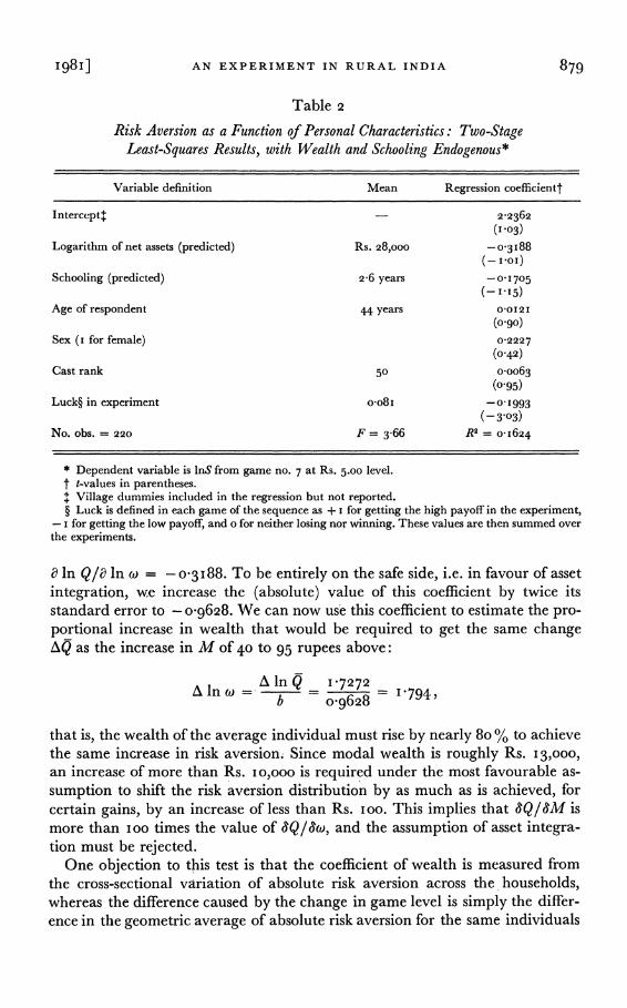
I98I] AN EXPERIMENT IN RURAL INDIA 879
Table 2
Risk Aversion as a Function of Personal Characteristics: Two-Stage Least-Squares Results, with Wealth and Schooling Endogenous*
Variable definition Mean Regression coefficientt
Intercept+ 2-2362 (103)
Logarithm of net assets (predicted) Rs. 28,000 -0 3 I88 (- IOI)
Schooling (predicted) 2-6 years - 01705
(-1.15)
Age of respondent 44 years 00121
(0-90)
Sex (i for female) 0-2227
(o042)
Cast rank 50 o-oo63 (0.95)
Luck? in experiment oo8 I -0 1 993
(-3.03)
No. obs. = 220 F = 3-66 R2 = o-i624
* Dependent variable is InS from game no. 7 at Rs. 5.00 level. t t-values in parentheses. + Village dummies included in the regression but not reported. ? Luck is defined in each game of the sequence as + i for getting the high payoff in the experiment,
- i for getting the low payoff, and o for neither losing nor winning. These values are then summed over the experiments.
a In Q/l In 0) = -o03 I88. To be entirely on the safe side, i.e. in favour of asset integration, we increase the (absolute) value of this coefficient by twice its standard error to - o9628. We can now use this coefficient to estimate the pro- portional increase in wealth that would be required to get the same change AQ as the increase in M of 40 to 95 rupees above:
Alw ln Q 1 P7272 = . i\ In cl)- b 0 o 9628 794,
that is, the wealth of the average individual must rise by nearly 8o % to achieve the same increase in risk aversion; Since modal wealth is roughly Rs. 13,000,
an increase of more than Rs. io,ooo is required under the most favourable as- sumption to shift the risk aversion distribution by as much as is achieved, for certain gains, by an increase of less than Rs. ioo. This implies that aQ/lM is more than ioo times the value of Q/1&), and the assumption of asset integra- tion must be rejected.
One objection to this test is that the coefficient of wealth is measured from the cross-sectional variation of absolute risk aversion across the households, whereas the difference caused by the change in game level is simply the differ- ence in the geometric average of absolute risk aversion for the same individuals

880 THE ECONOMIC JOURNAL [DECEMBER
across the game scale. (Note that the difference across game scales is statistically significant at the I % level.) Little can be done about this objection with the data used here.'
III. MODELS BASED ON SECURITY MOTIVES
A number of authors have proposed safety-based rules of thumb to describe and predict an individual's behaviour under risk. Anderson (1979) has recently reviewed these rules, and it is his exposition that we will follow here.
The advocates of safety-based rules of thumb usually propose these rules on the following grounds: (i) relative to utility-based models, they simplify the calculations the individual must make in order to decide among a set of alterna- tive actions; and (2) they offer a more realistic description of the individual's decision-making process than do utility-based models. Very rarely, however, do the proponents consider the information requirement of the analyst who attempts to make predictions for an individual or a group of individuals. How much does the analyst have to know about individual's tastes, opportunity sets, and constraint sets ? As we shall see, the distinction between the analyst's and the individual's information requirement is particularly important for safety- based rules. Individuals will usually know their subsistence needs, but an analyst may have to elicit information about these needs in order to make predictions. The same holds for other elements of individuals' tastes and constraints. There- fore, in addition to criteria (i) and (2), we will focus in this section on the analyst's information requirement.
Just as utility functions can be written in terms of net gains or in terms of wealth, so safety-based rules can be defined in terms of gains and losses arising from a simple prospect, or in terms of final income, which is the sum of the initial income stream and the net.gain from the new prospect (income integra- tion). In so far as income is the rate of return to an individual's physical and human capital, income and asset integration are identical concepts. Safety- based predictions differ sharply, depending on whether or not income integra- tion is assumed, and it will be shown that the analyst requires much more in- formation to derive predictions when income integration is assumed than when it is not. It should also be noted that targets for gains and losses arising from a specific set of prospects such as the experiment cannot be justified on the basis of subsistence incomes or physiological need considerations. Such con- cepts must be defined over total income, since gains from different sources are fungible in meeting these targets. Gain and loss targets would be appropriate only if individuals wanted to use gains from specific sets of prospects to purchase a desired good over and above some 'normal' expenditure level (for example, purchasing consumer durables, taking a trip).
Four rules are described in Table 3. They are written out in gain and loss form. The income-integrated form simply substitutes income I and income tar-
1 In Binswanger et al. (I980), a different measure of risk aversion, similar to an insurance premium, is used extensively in regression analysis. The model presented here was also estimated by use of the insurance premium, and there was no change in the nature of the results.

00 001
10 4-J 4) bo 0 0 0
0 Cd >
13 4-J
cis 4-J
ho
4) cis 0 0 4-J WD 4 4
m 0 cis $4 cis
$4
> 1-4
0 0
&4 &4
.4 4-J 4-J 4-J 0 0
biD cis > >
rA v
0
cis
-4 '04> oI +.a 04
4-4 14 ..4 -4 CIS CIS
4-J O 9 0 $4 cis $4 cis
-$i 0 04 04O 4) t..4 biD C.' b4O
10 04 0 0
4-4 0 cd cd
$.4 0 Cdu 04
cd
04 4-4 cd a,
0 .0 4 &.
.4 $-44 4-4
0
4-J4
0 0 P4 Cd cis
4-J cis bo bo
Cd CIS 4-J r Gn 0 0
cis Cd 0 0
1-4 -W C-d $4 $4
04 WD 0 tLo 4j
0 4-J0 0
C.. >
4-J cd 4-J Cd
0 4-4
bo 0 0 4-1 4-1
4-J 4-1 cis
M 4-1 4-J
,uj 4- bo ..4
cis 0 $4 U)
LrG cd rA
4-4 4-J 0 4-J0
CIS
4-J 0 cd
0 0 e-, rA
5 'a
F) r, 4-J cis Cd 0
4-4o .4
C4.4 4-J 4-J Cd cis Wz! 0 -0 .4 0 bo 0 bo
CIO 4-4 CIS tO V
4-1
Qd 4J 0 bo
0 > Cd cd u Cd .4 43 0 4) cd cd u 4)
$4 4- $4 4-4 $-4 4-J rA
C'd
4-J
blo
cis 4-A
A- 4-4
0 0 0 u : N.;,u
t:2 ..4 U
be
co U)
uC= 0- U
$.4
C's 4-J 4-J
4-1 4-4
04 Cd Cd 0 cn
Cd 4-1 4-1 Cd V Cdqcn
0 .04 0
'.0 cd u
x Cd Cd p
to b. :J -6
O .-
4-J 4-J tg .
u U Cd cn 0 4-1 0 -4 v
>,. j
cd 4-J 4-J
Cd Cd Cd Cd cd Cd0 Cd
-4
cd to
to
cd Cd bo
cd cl u s-4
P >1 u Cd > -, u .. Cd
Cd C0.4
Cd Cd 4 .,
Cd
cd Cd
1-4

882 THE ECONOMIC JOURNAL [DECEMBER
get D* for gain X and gain target d* (see Table 3, row 6). Thus the rules will be discussed in gain and loss form only.
Safety-fixed Rule (Table 3,, row I). The individual is assumed to choose the prospect that maximises the minimum gain d achievable with a fixed probability (i - P*). P* is the target probability of disaster. When P* is equal to zero, the rule is called Maximin, meaning maximise the minimum gain.
Safety Principle Rule (Table 3, row 2). Instead of being concerned largely with the target probability, here the individual is assumed to be most interested in a target gain level d* and to choose the prospect that will maximise tne proba- bility that the actual gain will exceed the target or disaster gain level d*.
Lexicographic Rules (LSF) (Table 3, rows 3 and 4). Roumasset (I973) has pro- posed two lexicographic rules that are designed to sharpen the predictions. These rules operate with both a fixed probability target and a fixed gain (income) target and assume that the individual first wants to satisfy the safety constraint in row 5. This constraint says that the individual will only want to accept alter- natives that give him or her a target gain d* with a fixed target probability ( P*).
When the constraint is satisfied, the individual will choose the alternative that maximises the expected gain (or income); that is, the rules break ties between those alternatives that satisfy the safety constraint.
LSF-2 and LSF-i differ only in their predictions of what the individual will do when none of the alternatives satisfies the safety constraint. Under LSF-2, the individual will behave in the safety-fixed fashion; under LSF-i, the indi- vidual will behave according to the safety principle.
Predictions with Gain and Loss Targets In what follows we will consider predictions only for probability target P* of less than I /2, since proponents of such rules would surely not have thought of disaster probability targets greater than that.
It is clear from inspecting the set of experimental payoffs in panel I of Table I
that any decision maker using the safety fixed rule (Table 3, row I) must choose alternative zero at all game levels since that results in the highest bad luck income for any P* in the interval o < P* < I/2. In panel II of Table I
we see that at best 2-5 % of individuals have chosen alternative zero; the safety- fixed rule therefore does not describe observed behaviour.
The other three rules in Table 3 are tested as follows. In conjunction with an observed distribution of choices, each rule implies restrictions on the distribution of target incomes among the respondents. For example, only a limited range of target incomes may be consistent with the observed choices. Since the games have been played at several levels, the distribution of choices at each level can be used to derive independent predictions about the distribution of target gains. If these predictions are inconsistent across game scales, the majority of individuals cannot have behaved according to the decision rule used to derive the predictions.
The left-hand column of Table 4 lists 3I ranges of target gains. These ranges span the potential gains achievable in the experiment. Columns (I)-(4) give

I98I] AN EXPERIMENT IN RURAL INDIA 883
Table 4
Choice Sets at Various Levels of Target Incomes and Various Game Levels under the Alternative Safety-based Rules with Gain and Loss Targetst
Rules (in rupees)
Safety principle LSF-2
Game level Rs. 0.50 level Rs. 50.00 level Rs. o.5o level Rs. 50.00 level (range of d*; in rupees) (I) (2) (3) (4)
o0oo < d* < o-Io OABCE OABCE E E O0io < d* S 0?30 OABC C 0o30 < d* S 0?40 OAB B 040 < d* < 045 OA A 045 < d* S 0*50 0 0 0o50 < d* S 0?95 ABCEF 0o95 < d* < I-oo BCEF I-00 < d* < 1-20 BCEF 1-20 < d* S 150 CEF I*50 < d* < I-90 EF I-90 < d* < 2-00 F
20 oo< d* S 3o00 No prediction 3o00 < d* S 4o00 (all alternatives) 4o00 < d* < 4*50 450 < d* < 500 5o00 < d* < 9*50 9 50 < d* < Io-oo OABCE E
10o00 < d* S I2oo OABC C 12*00 < d* < 15o00 C 15-00 < d* < I9-00 C i9o00 < d* < 20-00 C
20 < d* S 30 OABC C 30 < d* S 40 OAB B 40 < d* S 45 OA A 45< d* S 50 0 0 50 < d* S 95 ABCEF 95 < d* < 120 BCEF
120 < d* S I50 CEF I50 < d* < I90 EF I90 < d* < 200 F 200 < d* No prediction 0 0
t Alternatives included in eaclh set are preferred to eveiy excluded alter-native, and the decision maker is indifferent among all alternatives included in the set.
the set of choices an individual can make, following either of the two rules indicated. Alternatives included in the choice sets are preferred to every excluded alternative, and the decision maker is indifferent among all alternatives included in a set. We assume also that indifference implies random choice; that is, each alternative included in the set has an equal probability of being selected. With- out this assumption of indifference, we could make few predictions about dis- tributions of target incomes.
The safety principle implies no prediction wlhenever the target gain cannot
884 THE ECONOMIC JOURNAL [DECEMBER
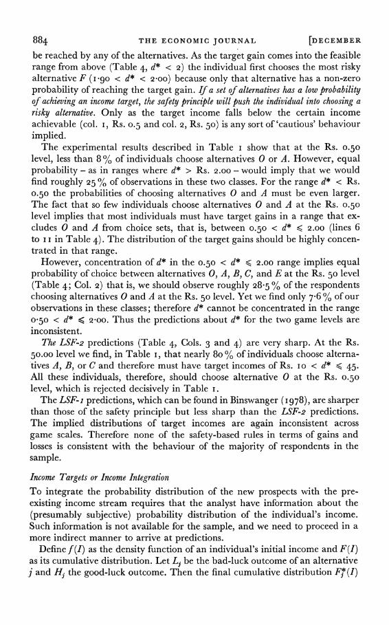
be reached by any of the alternatives. As the target gain comes into the feasible range from above (Table 4, d* < 2) the individual first chooses the most risky alternative F (i g90 < d* < 20oo) because only that alternative has a non-zero probability of reaching the target gain. If a set of alternatives has a low probability of achieving an income target, the safety principle will push the individual into choosing a risky alternative. Only as the target income falls below the certain income achievable (col. I, Rs. o.5 and col. 2, Rs. 50) is any sort of 'cautious' behaviour implied.
The experimental results described in Table I show that at the Rs. 0.50 level, less than 8 % of individuals choose alternatives 0 or A. However, equal probability - as in ranges where d* > Rs. 2.00 - would imply that we would find roughly 25 % of observations in these two classes. For the range d* < Rs. 0.50 the probabilities of choosing alternatives 0 and A must be even larger. The fact that so few individuals choose alternatives 0 and A at the Rs. 0.50 level implies that most individuals must have target gains in a range that ex- cludes 0 and A from choice sets, that is, between 0.50 < d* < 2.00 (lines 6 to I I in Table 4). The distribution of the target gains should be highly concen- trated in that range.
However, concentration of d* in the 0.50 < d* < 2.00 range implies equal probability of choice between alternatives 0, A, B, C, and E at the Rs. 50 level (Table 4; Col. 2) that is, we should observe roughly 28-5 % of the respondents choosing alternatives 0 and A at the Rs. 50 level. Yet we find only 7-6 % of our observations in these classes; therefore d* cannot be concentrated in the range oso < d* < 20oo. Thus the predictions about d* for the two game levels are inconsistent.
The LSF-2 predictions (Table 4, Cols. 3 and 4) are very sharp. At the Rs. 50.00 level we find, in Table i, that nearly 8o % of individuals choose alterna- tives A, B, or C and therefore must have target incomes of Rs. IO < d* < 45. All these individuals, therefore, should choose alternative 0 at the Rs. o.5o level, which is rejected decisively in Table I.
The LSF-i predictions, which can be found in Binswanger (I978), are sharper than those of the safety principle but less sharp than the LSF-2 predictions. The implied distributions of target incomes are again inconsistent across game scales. Therefore none of the safety-based rules in terms of gains and losses is consistent with the behaviour of the majority of respondents in the sample.
Income Targets or Income Integration To integrate the probability distribution of the new prospects with the pre- existing income stream requires that the analyst have information about the (presumably subjective) probability distribution of the individual's income. Such information is not available for the sample, and we need to proceed in a more indirect manner to arrive at predictions.
Define f (I) as the density function of an individual's initial income and F(I) as its cumulative distribution. Let L3 be the bad-luck outcome of an alternative j and Hj the good-luck outcome. Then the final cumulative distribution Fj (I)

I98I] AN EXPERIMENT IN RURAL INDIA 885
of income (which integrates the income from choice alternative j into the pre- existing income stream) becomes
Fj* (I) = IF (I - Hj) + IF (I - Lj) * ( I 5)
The basic feature of the final cumulative probability functions FO to FE is that they, cross each other before or when they reach P = I/2.
Good-luck H F outcome 200 E
C
B
100 A
0 50
I I I
10 30 50 L
Bad-luck outcome
Fig. 2. Relationship between bad-luck outcome and good-luck outcome of experimental alternatives 0 to F.
Without income integration, the safety-fixed rule implies choice of alterna- tive 0 in all cases where P* < I/2. But with income integration, the choice depends on target probabilities. When these are very low, the riskless alterna- tives will be chosen. As they rise, the choice shifts to more and more risky alter- natives. I am unable to derive predictions about the behaviour of individuals for any of the game levels. Hence, the rule cannot be falsified by the present experiment. A new experiment that could falsify it would have to elicit personal probability targets and personal probability distributions of overall income. Because eliciting certainty equivalents by interview is difficult (see Binswanger, I980), the prospects either for falsification or for support of this model are not good.
To consider the other rules, we neglect the discrete nature of the choices.' In Fig. 2, the good-luck Houtcomes of the experimental alternatives are plotted
1 The model that follows assumes either that the set of choices is continuous, as described in Fig. 2, or that linear combinations of the choices are possible. In the latter case, the function of Fig. 2 would approximate a piecewise linear set of choices. The present experiment fulfils neither of these conditions, but it is not clear why the discontinuities implied in the experiment should lead to more than random errors.

886 THE ECONOMIC JOURNAL [DECEMBER
as a function of the bad-luck outcomes L. There will exist some smooth, de- creasing convex function H= g(L) that fits these points exactly and in its range of definition o < L < 50 has the following properties: g (L) > L, g'(L) < - I, g"(L) < o. Furthermore, we can associate a factor k with each game level, that is, k(o) =I, k(5) = I/ I, k(o.so) I / 100 and thus represent all functions (i.e. all game options) derived from the distribution of initial income F(I) by the following distribution (which is a function of only the choice variable L and the scale parameter k):
F*(I) = F[I-kg(L)] +F(I- kL). (i6)
For any given game level (or scale factor k) the safety principle with final income target D* then implies the following maximisation problem over L:
Max [I-F*(D*)] = Prob (I > D*). (I7) L
Readers can verify for themselves - by minimising equation (I6) with respect to L and solving for first and second order conditions - that this problem can have an interior maximum for a wide variety of distributions, game levels, and target incomes. Furthermore, by solving for displacements one can obtain the derivatives required for predictive purposes, namely, dL/dD* and dL/dk. These derivatives would predict the direction of shifts in choices as target incomes or game levels rise, but these derivatives cannot be signed in the absence of quantitative knowledge of the second derivatives for the cumulative distribution F(I) of preexisting income. The information requirements for predictive pur- poses are very complex. When they are not met, predictions can only be made if one is willing to base the notion of target income on physiological subsistence requirements. In such a case, variations in the target income have a clear inter- pretation: Poor people should have high subsistence incomes and rich people low ones, relative to theirfinal probability distribution of income. This implies that poor people should have high probabilities of not achieving their subsistence income, whereas rich people should have low ones. Therefore, at least at low game levels, we should observe some poor- people choosing the risky alternatives E and F and rich people choosing the less risky ones, 0, A, and B. Yet the evidence reported in Binswanger (I980) is to the contrary. At the lowest game levels the rich tend to play more risky games than the poor, while at the higher game levels poor and rich tend to make very similar choices.
Equation (i 6) has clearer predictive implications for the lexicographic rules: for any given L (which defines a choice alternative), the final cumulative proba- bility distribution shifts to the right as the game level rises. This can be shown by differentiating equation (i6) with respect to k, that is,
t9F* (I)- 1 =
- -lh[I-kg(L)]g(L) -lh(I-kL)L < o, (i8)
where h refers to the density functions (with values greater than or equal to zero). This implies that, at a given target income D*, the probability of not reaching the target will fall for each alternative 0 to F as the game level rises.

I98I] AN EXPERIMENT IN RURAL INDIA 887
Furthermore, any alternative that satisfies the constraint at a low game level must also do so at every higher level. If an individual, for example, chooses alternative C at the Rs. 0.50 level because it maximises expected income over that set, the individual cannot, at a higher game level, move to a less risky alternative 0, A, or B (since C will not leave the set of alternatives which satisfies the safety constraint). If alternatives 0 and A are not members of that set at the Rs. 0.50 level but become so at higher levels, the maximisation of expected income would still imply choice C. On the other hand, additions of alternative E or F, at higher g-ame levels, to the set that satisfy the safety constraint would result in a switch from C to E or to F at these levels. This means that we should observe a shift in the distribution toward risk neutrality as the game level rises.' Yet the trend in the experimental results is a statistically significant movement away from the risk-neutral choices. Thus, the evidence is inconsistent with both lexicographic rules.
IV. DISCUSSION
Several security-based models of behaviour under risk have been shown to predict results with respect to simple decision making that are inconsistent with the experimental evidence from a large-scale experiment. The only security-based models that are not inconsistent with the experimental evidence are the safety-fixed model with income integration and the safety principle with income integration (although the latter is also inconsistent when target incomes have a physiological-need interpretation). The reason for the survival of these two models is that they offer no prediction whatsoever unless personal probability targets (or income targets), and the subjective probability distribution of initial income, and its derivatives, are known. For the analyst these models are far from being less complicated than utility-based models, and until their advocates propose ways of measuring the necessary elements the models cannot be opera- tional.
One might object that the experiment discussed in this paper is not a good test because it does not subject the individual to losses. But such an objection can logically be made only for safety-based rules in gains and losses, since income integration implies that all opportunity losses are real losses. But the gains and loss rules are quite clearly rejected. Furthermore, we have shown elsewhere that, when people were given the money for a game one day in advance and thus had to bring it back in order to play and put it at risk, their decisions did not differ statistically from the ones they made when payouts were given only after a game was played (Binswanger 1980). Subjects treated opportunity losses much like real losses.
Utility theories also have ambitious information requirements. But the
1 This discussion does not exclude the possibility that individuals might shift from E and F to less risky alternatives (as game levels rise), provided that at low game levels none of the alternatives satisfies the safety constraint (as long as P* < 1/2). However, in our experiment we should observe many shifts in the opposite direction. In going from the Rs. 5 game to the Rs. 5o and the Rs. 500 games, only three cases of shifts towards risk neutrality can be found.

888 THE ECONOMIC JOURNAL [DECEMBER
experiment reported here allowed a direct measurement of the risk aversion coefficients of at least the gains branch of the utility function. And we have shown elsewhere (Binswanger et al. I 980) that these measures are indeed related to actual economic decisions of the individuals studied. Extensions of the ex- perimental approach such as those reported in Sillers (I980) probably allow one to measure the loss branch as well.
Tests concerning utility-based models were confined, by the nature of the experiment, to issues concerning utility functions. We find (i) decreasing abso- lute risk aversion; (2) increasing partial risk aversion; and (3) declining rather than increasing relative risk aversion as hypothesised by Arrow. However, the latter finding, as we have discussed, is not a rejection of utility theory but of an ad hoc assumption by Arrow.
The major finding with respect to utility models is that the assumption of asset integration is inconsistent with the experimental evidence reported, as well as with experimental evidence involving hypothetical questions reported by Kahneman and Tversky (I979). As Markowitz (I952) has hypothesised, decision makers apparently do not evaluate utilities of final wealth states but of changes in wealth, that is, utilities of gains and losses.'
As Kahneman and Tversky (I979) point out, rejection of asset (or income) integration opens the possibility that new prospects may be evaluated in diff- erent ways, depending on the reference point with respect to which a decision maker assesses the prospects. In certain situations this may lead to decisions that are inconsistent with some of the axioms of behaviour on which the sub- jective expected utility models of statistics and economics rest. Furthermore, since the experiment reported here was played only with positive payoffs, we cannot infer from this game the shape of the utility function for losses. We could have done this if asset integration had been accepted.
On the other hand, lack of asset integration does not severely restrict our ability to derive comparative static predictions of behaviour under risk. First, we have the important finding that, at higher than trival payoffs levels, partial risk aversion of all individuals is concentrated in a narrow range and is fairly constant. In many instances the use of an average partial risk aversion (or narrow lower and upper bounds) will be sufficient to predict behaviour accur- ately regardless of the wealth levels of the individuals.
Furthermore, if one is also interested in the effects of minor variations in risk aversion that are associated with wealth, not only does the experiment give estimates of partial risk aversion at different game levels but the regression results indicate how partial risk aversion changes as wealth rises.
1 The finding of declining relative risk aversion and the rejection of asset integration (or stability of the utility function over time) are intimately related and rest on the fact that the observed behaviour of individuals at low game levels is extremely cautious relative to their assets. Consider the individual choosing game B at the Rs. 5-00 level, with low and high outcomes of Rs. 4 and 12. Alternative A, on the other hand, would give the individual Rs. 3.oo and Rs. I5.oo. The individual is unwilling to risk a loss of Rs. i.oo with 50% probability in order to increase his expected income by Rs. i.oo. If the individual's wealth is Rs. io,ooo (close to the mode in the sample), then the loss with 50 % probability is only i / i ooooth of his or her wealth. Choosing the same alternative at the Rs. 500 level implies a much higher risk relative to wealth. Stated otherwise, the curvature of the gains branch of the utility function is much larger at low levels of games than at high levels.

I98I] AN EXPERIMENT IN RURAL INDIA 889
A final point relates to methodology: All predictions that were used as tests against the experimental evidence for the different models of behaviour were predictions about changes in behaviour as the level of the game rises from the Rs. 0.50 to the Rs. 50 level. For any given set of theoretical assumptions a single game level could have been used to derive a measure of risk aversion at that level, but different theories could not then have been tested against each other. Psychological experiments often use no real payoffs or payoffs that are scaled around a single level. It appears that such experiments could gain greatly in discriminatory power by introducing much greater variation in payoffs than has usually been the case. The experimental costs of doing this may increase, buj they may not be higher than the costs of alternative research strategies using sample surveys and/or vast amounts of computer resources.
The World Bank
Date of receipt offinal typescript: May 1981
REFERENCES
Anderson, Jock R. (I979). 'Perspective on models of uncertain decisions.' In Risk Uncertainty and Agricultural Development (ed. J. A. Roumasset, J. Boussard and I. Singh). College, Laguna, Philip- pines and New York: SEARCA and Agricultural Development Council, Inc. Dillon, John L. and Hardaker, Brian (I977). Agricultural Decision Analysis. Ames: Iowa State
University Press. Arrow, Kenneth H. (197I). Essays in the Theory of Risk Bearing. Amsterdam: North Holland. Binswanger, Hans P. (I 978). 'Attitudes toward risk: implication for economic and psychological theories
of an experiment in rural India.' Discussion Paper 286, Yale University, Economic Growth Centre. (I980). 'Attitudes toward risk: experimental measurement in rural India.' American Journal of
Agricultural Economics, vol. 62, no. 3 (August), pp. 395-407.
Jha, Dayanatha, Balaramaiah, T. and Sillers, Donald (I980). 'The impacts of risk aversion on agricultural decisions in semi-arid India.' International Crops Research Institute for the Semi-Arid Tropics, Hyderabad, India. Mimeo.
Edwards, Ward (1953). 'Probability-preferences in gambling.' American Journal of Psychology, vol. 66
(July), PP. 349-64. (I954). 'The reliability of probability-preferences.' American Journal of Psychology, vol. 67 (March),
pp. 68-95. ((I955)). 'The prediction of decisions among bets.' Journal of Experimental Psychology, vol. 50 (Sep-
tember), pp. 201-14.
Fishburn, Peter C. (1978). 'On Handa's "New Theory of Cardinal Utility" and the maximisation of expected returns.' Journal of Political Economy, vol. 86 (April), pp. 321-4.
Friedman, Milton and Savage, Leonard J. (1948). 'The utility analysis of choices involving risk.' Journal of Political Economy, vol. 56 (August), pp. 279-304.
Grether, David M. (1978). 'Recent psychological studies of behaviour under uncertainty.' American Economic Review, vol. 68, no. 2 (May), pp. 70-4.
Griffith, R. M. (I964). 'Odds adjustment by American horse race bettors.' American Journal of Psy- chology, vol. 62 (July), pp. 387-98.
Halter, Albert, N. and Dean, Gerald W. (I97I). Decisions under Uncertainty with Research Applications. Cincinnati: South-Western Publishing Co.
Handa, Jagdish (I977). 'Risk, probability and a new theory of cardinal utility.' Journal of Political Economy, vol. 85 (February), pp. 97-122.
Hildreth, Clifford (I974). 'Ventures, bets and initial prospects.' In Decision Rules and Uncertainty (ed. Michael Balch, Daniel McFadden and S. Wu). Amsterdam: North Holland.
Kahneman, Daniel and Tversky, Amos (1979). 'Prospects theory, an analysis of decision under risk.' Econometrica, vol. 47, no. 2 (March), pp. 263-9I.
890 THE ECONOMIC JOURNAL [DECEMBER I98I]
Luce, Duncan R. and Suppes, Patrick (I965). 'Preference, utility and subjective probability.' In Handbook of Mathematical Psychology (ed. Duncan R. Luce, Robert R. Bush and Eugene Galanther). New York: John Wiley.
Markowitz, Harry (1 952). 'The utility of wealth.' Journal of Political Economy, vol. 6o (April), pp. 15I-8.
Menezes, C. F. and Hanson, D. L. (I970). 'On the theory of risk aversion.' International Economic Review. vol. i i (October) pp. I81-7.
Preston, Malcolm G. and Baratta, Philip (1948). 'An experimental study of the auction-value of an uncertain outcome.' American Journal of Psychology, vol. 6i (April), pp. 183-93.
Ramsey, Frank P. (I 93 I) . 'Truth and probability.' I 926. In The Foundations of Mathematics and Other Logical Essays (ed. F. P. Ramsey). New York: Harcourt, Brace.
Rothschild, M. and Stiglitz, J. E. (I970). 'Increasing risk. I. A definition.' Journal of Economic Theory, vol. 2, No. 3, pp. 66-84.
Roumasset, James (I 973) . 'Risk and choice of technique for peasant agriculture: the case of the Philip- pine rice farmers.' Ph.D. dissertation, University of Wisconsin, Department of Economics.
Savage, Leonard J. (I 954). Foundations of Statistics. New York: John Wiley. Sillers, Donald A. (i980). 'Measuring risk preferences of rice farmers in Nueva Ecija, the Philippines:
An experimental approach.' Ph.D. dissertation, Yale University, Department of Economics. Sprowls, R. C. (I953). 'Psychological-mathematical probability in relationships of lottery gamblers.'
American Journal of Psychology, vol. 66 (January), pp. 125-30.
Von Neumann, James and Morgenstern, Oskar (I947). The Theory of Games and Economic Behaviour. Princeton, N.J.: Princeton University Press.
Tversky, Amos (1 967). 'Additivity, utility and subjective probability.' Journal of Mathematical Psychology, vol. 4 (June), pp. 175-201.
Zeckhauser, Richard and Keeler, Emmett (1970). 'Another type of risk aversion.' Econometrica, vol. 38 (September), pp. 66I-5.