ATTITUDE CONTROL OF A BIO-INSPIRED ROBOTIC FISH WITH FLEXIBLE PECTORAL FINS

by

Lijuan Pi

A thesis submitted to the Faculty of the University of Delaware in partial fulfillment of the requirements for the degree of Master of Science in Mechanical Engineering

Fall 2009

Copyright 2009 Lijuan Pi All Rights Reserved

ATTITUDE CONTROL OF A BIO-INSPIRED ROBOTIC FISH WITH FLEXIBLE PECTORAL FINS

by

Lijuan Pi

Approved: __________________________________________________________ Xinyan Deng, Ph.D. Professor in charge of thesis on behalf of the Advisory Committee Approved: __________________________________________________________ Anette M. Karlsson, Ph.D. Chair of the Department of Mechanical Engineering Approved: __________________________________________________________ Michael J. Chajes, Ph.D. Dean, College of Engineering Approved: __________________________________________________________ Debra H. Norris, M.S. Vice Provost for Graduate and Professional Education

iii

ACKNOWLEDGMENTS

I would like to thank my advisor, Professor Xinyan Deng, for giving me

the opportunity and support to work on the new area of bio-inspired robotic fish. It has

been a great experience for me to work with her to explore inspiring design and

control problems to address in this field.

I wish to thank Professor Liyun Wang and Professor Bert Tanner for

serving on my thesis committee. Their comments and advice helped improved my

manuscripts and presentations.

My labmate, Liang Zhao, has been a great help on the fluid mechanics

aspects of my research through our various discussions. Zhen Hu and Qingfeng

Huang offered a lot of help on the boxfish shell experiment. Bo Cheng always discuss

with me on the control problems, his idea inspires me a lot. Ray and Steve’s help

make it easier to build the robotics fish platform. I would like to thank them all.

I must thank all my family members; your love supports me through my

studies. You are the best treasure I can ever dream of.

iv

TABLE OF CONTENTS

LIST OF TABLES ....................................................................................................... vii LIST OF FIGURES ..................................................................................................... viii ABSTRACT .................................................................................................................. xi CHAPTER 1 INTRODUCTION ............................................................................................ 12

1.1 Classification of fish swimming modes .................................................. 12 1.2. Classification and function of fins ........................................................... 13 1.3. Overview of robot fish design ................................................................. 14 1.4. Overview of pectoral fin research ........................................................... 16 1.5. Contributions of this thesis ...................................................................... 17 1.6. Thesis outline ........................................................................................... 18

2 EXPERIMENTAL PLATFORM OF THE ROBOTIC FISH .......................... 19

2.1. Schematic of the system .......................................................................... 19 2.2. Fish body prototype ................................................................................. 21

2.2.1. Fin design and degree of freedom ............................................... 22 2.2.2 Mechanical chassis design ........................................................... 25 2.2.3 Actuators ..................................................................................... 28 2.2.4 On board power converter ........................................................... 29 2.2.5 On-board Sensors ........................................................................ 30

2.3 Computer-based experimental platform .................................................. 32

2.3.1 PCI-6229 DAQ board .................................................................. 32 2.3.2 SCB-68 connector blocks and input/ output mode ...................... 33 2.3.3 Analog input port and Digital output ports ................................. 34

3 SENSOR ARRANGEMENT AND DATa COLLECTING ............................ 36

3.1 Global coordinates and body fixed coordinates ...................................... 36 3.2 Sensor axis alignment, calibration and filtering ...................................... 38

v

3.2.1 Sensor axis alignment .................................................................. 38 3.2.2 Sensor calibration ........................................................................ 40 3.2.3 Sensor signal acquisition and pre-processing .............................. 42

3.3 Conclusion ............................................................................................... 43

4 SENSOR FUSION ALGORITHEM AND EXPERIMENTAL RESULT ...... 44

4.1 Kalman filter algorithm based on Quaternion algebra [64, 66] ............... 44

4.1.1 Basic concept of Quaternion method [64, 66, 67] ....................... 44 4.1.2 Quaternion angular velocity integral .......................................... 46 4.1.3 Translate quaternion to Rotation matrix Euler angle .................. 46 4.1.4 Kalman filter for attitude estimation [66] .................................... 47 4.1.5 Attitude estimation Stage (integrating angular rate) ................... 48 4.1.6 Update Stage (eliminating estimate error) ................................... 49 4.1.7 Kalman filter implementation ..................................................... 51

4.1.7.1 Kalman filter experimental setup ................................. 53 4.1.7.2 Experiment results ........................................................ 55

4.1.8 Conclusion ................................................................................... 56

4.2 Complementary filters based on Lie algebra [65] ...................................... 59

4.2.1 Basic definitions [65] .................................................................. 59 4.2.2 Complementary filter algorithm .................................................. 60 4.2.3 Numerical Implementation .......................................................... 61 4.2.4 Experimental Tests of Attitude Estimation ................................. 61

4.2.4.1 Experimental Setup ...................................................... 61 4.2.4.2 Results .......................................................................... 63

5 ATTITUDE CONTROL WITH FLEXIBLE PECTORAL FINS .................... 67

5.1 Flexible pectoral fin ................................................................................. 67

5.1.1 Hydrodynamics forces on flapping fins ...................................... 68 5.1.2 Lift force and drag force .............................................................. 69 5.1.3 Fin material and angle of attack .................................................. 71 5.1.4 Pectoral fin shape design. ............................................................ 74

5.2 Roll plane dynamics of robotic fish ......................................................... 76

5.2.1 Simplified moment equation ....................................................... 76

vi

5.2.2 Control variable of pectoral fins .................................................. 78 5.2.3 Simplified roll-axis dynamics model .......................................... 80 5.2.3 System model identification ........................................................ 81

5.3 PD Controller design for robot fish fixed on holder ................................ 85 5.4 PD controller for rolling angle tracking of free robot fish ...................... 91 5.5 Conclusion ............................................................................................... 94

6 CONCLUSIONS AND FUTURE WORK ....................................................... 95

6.1 Summary of the work presented .............................................................. 96

6.1.1 Robotic Prototype and flexible pectoral fin design ..................... 96 6.1.2 Sensor fusion for attitude estimation ........................................... 97 6.1.3 Roll motion dynamics modeling and linear control .................... 97

6.2 Future Work ............................................................................................. 98

6.2.1 3-DOF flexible pectoral fin ......................................................... 98 6.2.2 Wireless signal transmit and more sensors .................................. 98 6.2.3 Fin-fin interaction and complex control ...................................... 98

APPENDIX SAMPLE CODE OF KALMAN FILTER AND PD CONTROL .............................. 100 SOFTWARE USER INTERFACE ............................................................................ 103 REFERENCE ............................................................................................................. 104

vii

LIST OF TABLES

Table 2.1 Output channel assignment for fish prototype I ...................................... 34

Table 2.2 Output channel assignment for fish prototype II ..................................... 35

Table 2.3 Input channel assignment for fish prototype I ......................................... 35

Table 2.4 Input channel assignment for fish prototype II ........................................ 35

viii

LIST OF FIGURES

Fig. 1.1. Fish classification scheme based on swimming mode [1]. ................... 13

Fig.1.2. Bluegill sunfish showing the configuration of median and paired fins [2]. ................................................................................................... 14

Fig. 2.1. Schematic of the system. ........................................................................ 20

Fig. 2.2. Physical appearance of the experimental system. .................................. 21

Fig.2.3.a) Fish’s pectoral fin ................................................................................... 22

Fig. 2.3 b) Pectoral fins with definition of flapping , rowing , and feathering angles ................................................................................ 23

Fig. 2.4 Control signals of flapping and rowing for prototype I.......................... 24

Fig. 2.5 Fish robot prototype I ............................................................................. 26

Fig.2.6 Fish robot prototype II. ........................................................................... 27

Fig. 2.7 Control pulse for servo motors ............................................................... 29

Fig.2.8 LM317 and voltage converter circuit . ................................................... 30

Fig. 2.9 Circuit diagram of Breakout board of ADXL330 [99]. ......................... 31

Fig. 2.10 Circuit diagram of Breakout board of IDG300 [100] . .......................... 31

Fig.2.11 PCI-6229 board [101]. ............................................................................ 32

Fig. 2.12 NRSE Analog input mode. ..................................................................... 33

Fig.2.13 Servo arrangement of fish prototype I & II ............................................ 34

Fig. 3.1 Global coordinates and body fixed coordinates ..................................... 37

Fig. 3.2 Alignment of two sensors in the robotic fish. ........................................ 39

Fig. 3.3 Three-DOF Mechanical holder [65] ....................................................... 42

ix

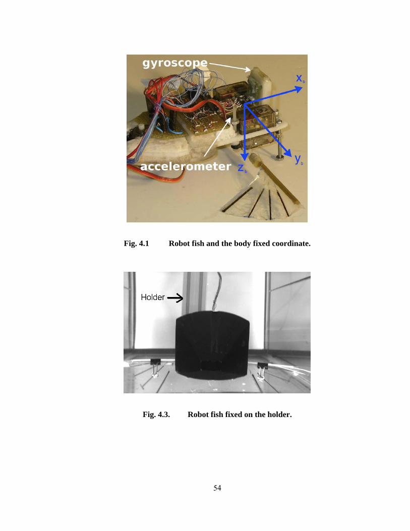
Fig. 4.1 Robot fish and the body fixed coordinate. ............................................. 54

Fig. 4.3. Robot fish fixed on the holder. ............................................................... 54

Fig. 4.3 Holder and MAE3 Encoder. ................................................................... 55

Fig. 4.4 Actual and estimated roll angle (t) for movements generated by external force. ......................................................................................... 56

Fig. 4.5 Actual and estimated roll angle (t) for movements generated by fin beats. ................................................................................................. 57

Fig. 4.6 Measured data from the sensors with fin flapping at 2Hz. ..................... 58

Fig. 4.9 The holder for roll/pitch motion and the body-fixed coordinate. ........... 62

Fig. 4.10 Comparison between the actual roll angle (top) and pitch angle (bottom) and three different estimations evaluated using the only accelerometers, the only gyroscopes data. ............................................. 65

Fig. 4.11 Accelerometers output (normalized with respect to gravity g) .............. 66

Fig. 4.12 3-axis gyroscopes output ........................................................................ 66

Fig.5.1 Robot fish with 1-DOF pectoral fins. ..................................................... 68

Fig. 5.2 Steady lift generation in a two dimensional foil. ................................... 69

Fig. 5.3 Forces on pectoral fin foil and angle of attack ....................................... 71

Fig.5.4 a) Drag coefficient of flexible foil as function of angle of attack [89]. ...... 73

Fig.5.4 b) Lift coefficient of flexible foil as function of angle of attack [89]......... 73

Fig.5.5 Three kind of fin shape and the cylindrical connector. .......................... 75

Fig.5.6 The robot fish with holder and sensors. ................................................. 76

Fig. 5.7 Definition of oscillating angle of pectoral fin. ....................................... 79

Fig.5.8 a) Validating result of ( )( )

sU s

by using white noise input. .................... 83

Fig.5.8 b) Validating results of ( )( )

sU s

by using sine-wave input ..................... 84

x

Fig.5.8 c) Validating results of ( )( )

sU s

by using sine-wave input. .................... 85

Fig.5.9 Schematic of control system of robot fish .............................................. 86

Fig.5.10 Bode plot of frequency response of open-loop system, close-loop system and the controller. ....................................................................... 89

Fig.5.11a) The roll angle stabilized at 180 degree. .................................................. 90

Fig.5.11b) The control variable u(t) used to stabilize the roll angle at 180 degree ..................................................................................................... 90

Fig.5.12 The roll angle of robot fish (with holder) tracking a sine-wave ............. 91

Fig.13a) The roll angle of robot fish stabilized at 20 degree. ............................... 92

Fig.13b) The roll angle of robot fish stabilized at 0 degree. ................................. 93

Fig.13c) Roll angle of robot fish tracking a sine-wave with magnitude of 45 degree ................................................................................................ 93

Fig.13d) Roll angle of robot fish tracking a sine-wave with magnitude of 75 degree ................................................................................................ 94

Fig.A.1 LABVIEW code of the whole control system ..................................... 101

Fig. A.2 LABVIEW code of Kalman filter ........................................................ 102

Fig.B.1 LABVIEW Interface for control system .............................................. 103

xi

ABSTRACT

Micro underwater vehicles (MUVs) have wide potential military,

scientific and commercial applications. They are especially suitable for exploring

dangerous and limited space. This thesis presents the development of a bio-inspired

MUV equipped with flexible fins and attitude measurement sensors. The pair of

flexible pectoral fins was driven by mini servo individually to mimic boxfish’s

pectoral fin motion. Two sensor fusion methods (Kalman filter based on quaternion

and Complementary filter based on Lie groups) was used to estimate robotic fish’s

rotational movement. A simplified dynamic model for the robot fish’s attitude control

was developed based on the theoretical analysis and experiment results. A linear PD

controller was designed to achieve the robot fish’s attitude stabilization in the roll axis

by controlling the flapping kinematics of the pectoral fins. Both simulation and

experiment results show convergence of roll angles in point-to-point control and

trajectory tracking of the desired motion.

12

Chapter 1

INTRODUCTION

Fish have obtained excellent swimming skills during the period of

evolution [2, 9]. Different fish swim modes have distinct advantages in speed,

maneuverability and efficiency. These advantages have encouraged researchers to

analyze the relation between fish morphology and locomotion style [9], and to apply

some characteristics of fish in the design of underwater vehicles.

1.1 Classification of fish swimming modes

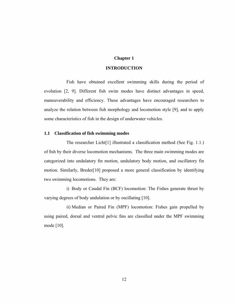
The researcher Licht[1] illustrated a classification method (See Fig. 1.1.)

of fish by their diverse locomotion mechanisms. The three main swimming modes are

categorized into undulatory fin motion, undulatory body motion, and oscillatory fin

motion. Similarly, Breder[10] proposed a more general classification by identifying

two swimming locomotions. They are:

i) Body or Caudal Fin (BCF) locomotion: The Fishes generate thrust by

varying degrees of body undulation or by oscillating [10].

ii) Median or Paired Fin (MPF) locomotion: Fishes gain propelled by

using paired, dorsal and ventral pelvic fins are classified under the MPF swimming

mode [10].

13

Fig. 1.1. Fish classification scheme based on swimming mode [1].

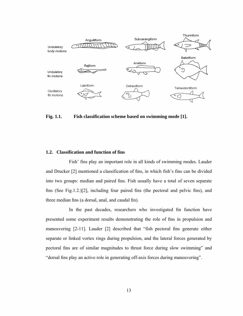
1.2. Classification and function of fins

Fish’ fins play an important role in all kinds of swimming modes. Lauder

and Drucker [2] mentioned a classification of fins, in which fish’s fins can be divided

into two groups: median and paired fins. Fish usually have a total of seven separate

fins (See Fig.1.2.)[2], including four paired fins (the pectoral and pelvic fins), and

three median fins (a dorsal, anal, and caudal fin).

In the past decades, researchers who investigated fin function have

presented some experiment results demonstrating the role of fins in propulsion and

maneuvering [2-11]. Lauder [2] described that “fish pectoral fins generate either

separate or linked vortex rings during propulsion, and the lateral forces generated by

pectoral fins are of similar magnitudes to thrust force during slow swimming” and

“dorsal fins play an active role in generating off-axis forces during maneuvering”.

14

Fig.1.2. Bluegill sunfish showing the configuration of median and paired fins [2].

Many researches are motivated to consider fish’s fins as a model for designing

propulsion component of different kinds of bio-mimetic autonomous underwater

vehicles [11-13]. Especially, some researchers indicated that the paired pectoral fins

produces lift and drag for efficient swimming and maneuvering, which might be

mimicked by underwater vehicle with flexible foils under complex motor control [14-

16].

1.3. Overview of robot fish design

The concept of mimicking the swimming features of fishes has led to

inventions in underwater vehicle designs that could have higher levels of performance

in speed, maneuverability, stability and energy efficiency. These bio- mimetic robot

15

fish may not only mimic the locomotion, morphology of a particular fish [2], but also

apply diverse fin designs, simplified motion kinematics, and intelligent control method

that are a result of experiments and computational fluid dynamics (CFD) simulations

[17-19]. In Bandyopadhyay’s article [20], the researcher reviewed the methods and

technology on biomimetic underwater vehicle design, including robot maneuvering by

using pectoral fins, high lift force fin hydrodynamics, actuators based on smart

material and bio-inspired control.

In the bio-mimetic robot fish field, MIT’s Robotuna designed by

Triantafyllou’s group [21-23] marks the first work of its kind. They employed the

carangiform locomotion in their robot design, followed by many bio-robotic fish

research based on carangiform model, including Caltech’s carangiform robot fish [24]

which were originally designed to analyze and test the hydrodynamic forces generated

by the 2 DOF tail fin. Other robot fish based on different swim locomotion have been

developed to analyze the features that might contribute to higher performance in

maneuverability, propulsion, or efficiency. In the research of Barrett [24], the result

indicated that robotic fish experienced less drag with undulatory motion than those

without body undulation. Researchers [23, 25] also analyzed the vorticity control

phenomenon of undulating body and tail fin, and the interactions between the body/tail

and the generated wake [26, 27]. In Licht [1]’s design, four heaving and pitching foils

were equipped to an underwater vehicle. Recently some fluid dynamics researchers

proposed an underwater vehicle design by combining the high efficient rigid tail foils

with flexible-ray pectoral fins for enhancing the maneuverability [28, 29].

It is apparent that the fin design and their interaction mode significantly

influence the robot fish’s swim performance. Particularly, pectoral fin has been

16

considered as a valued tool for underwater vehicle’s turning and maneuvering

performance [30-33].

1.4. Overview of pectoral fin research

In past years, researches have been conducted on pectoral fin morphology,

kinematics, hydrodynamics, and fin motion induced control surfaces [2, 29, 34]. Both

experimental and computational fluid dynamics (CFD) methods have been used as

tools to obtain the forces and torques produced by oscillating fins [2, 35-37]. Usually,

pectoral fins were mainly employed in two moving modes: flapping and rowing [32].

Pectoral fin generates lift-based-thrust force for propulsion by using flapping mode

[32, 33, 38]. Walker and Westneat [39] presented a hydrodynamic simulation result,

showing that flapping is more efficient in generating thrust than rowing. Fish

employed the rowing pectoral fins to generate a drag-based-thrust in the power stroke.

Walker and Westneat [40] also mentioned in their simulation result that rowing is

more effective for slow maneuvers. Kato [37] designed the latest 3 DOF pectoral fin

based underwater vehicle for low speed precise maneuvering. This 3DOF pectoral fin

can move in both rowing and flapping mode. Except rowing and flapping mode, some

experiments results indicate that pectoral fins using lead-lag and feathering mode

which can also produce large lift and thrust for control and propulsion of underwater

vehicles [14, 36, 41-43]

In underwater vehicle design, rigid foils are widely used to build the

mechanical pectoral fins [1, 36, 44-46]. Lauder [47, 48] built flexible pectoral fin by

using multiple rays and upporting base, and mimicking the muscle control. In addition,

flexible smart material has also been used to fabricate pectoral fins, and the related

hydrodynamics has been analyzed in experiment tests [49-51].

17

In the robot fish control, some researchers used the neural networks and

fuzzy controllers [45, 52, 53]. The design of open-loop and closed loop control

systems for the set-point regulation in the dive plane using optimal control has been

presented [5, 6, 54]. The inversion control technique provides a method for trajectory

tracking. Many experiment or simulation result about intelligent control has been

presented in the references [4, 55, 56]. Some researchers built the linear system model

for the robot fish by eliminating the unstable zeros of the original transfer function and

then conduct inverse control design [4, 7, 8]. This method has been used for the

pectoral fin control of a continuous time model of underwater vehicle [37, 57, 58].

In this thesis, we focus our research on sensor based attitude feedback

control of a robotic fish equipped with a pair of flexible pectoral fin driven by mini

servo motors. The purpose of our research is to validate the role of flexible pectoral

fin in robot fish’s attitude stabilization, to identify the dynamics model, and to use the

model in sensory feedback control.

1.5. Contributions of this thesis

This thesis presents the development of a centimeter scale MUV equipped

with flexible pectoral fin and orientation measurement sensors. The robot fish’s

attitude stabilization in the roll plane is attained by driving the pectoral fins under the

linear feedback controller.

In this work, the experiment results validated the possibility of using

flexible pectoral fin to control robot fish’s rolling maneuvering. Many researchers

have used mechanical pectoral fins as a device for underwater vehicle’s maneuvering

and stabilizing. These researchers were prone to use rigid foils to fabricate the pectoral

fins [37, 59]. In this thesis, the pectoral fin was built by flexible materials and the

18

characteristics of flexible pectoral fins were explored. In addition, some computational

fluid dynamics (CFD) groups, who simulated the AUV’s maneuvering with pectoral

fins, paid more attention to dive and yaw plane[4, 5], and neglect the roll plane. This

thesis focused on the attitude stabilization in roll plane which seems to be neglected by

previous researchers. Another contribution of this work is that the sensor fusion

experiments results presented in chapter 4 validate the new complementary filter

algorithm based on Lie group.

1.6. Thesis outline

Chapter 2 presents the design of sensor based robotic fish and the

corresponding computer-DAQ (Data acquisition) system. Chapter 3 presents the

definitions of coordinates, which are the basis of attitude estimation and stabilization

of robot fish. This chapter also describes sensor alignment and calibration method. In

Chapter 4, we describe two sensor fusion algorithms used for estimating the robot

fish’s attitude states. The algorithms include Kalman filter base on Quaternion algebra

and complementary filter based on Lie algebra. Experiment results validate these

sensor fusion methods. The estimated attitude state would be used in the linear

feedback control of robot fish. In Chapter 5, the simplified dynamic model of the robot

fish was developed. A proportional derivative (PD) feedback controller is

implemented to stabilize robot fish’s rotation in roll direction. The experiment results

validate the role of flexible pectoral fin in robot fish’s attitude stabilization. In addition,

the flexible fin design and the related hydrodynamics coefficient are also described.

The chapter 6 concludes the thesis and elaborates on the problems that are to be solved

and further control studies using the robotic prototype.

19

Chapter2

EXPERIMENTAL PLATFORM OF THE ROBOTIC FISH

This chapter presents the design of robotic prototypes of the MUV and the

related experiment platform. Two goals have been achieved in this part. One goal is to

design a small-sized robotic swimming machine, which can mimic the fish swimming

style. The other is to build a computer-based experimental platform to sense the

robot’s attitude state and to stabilize the robot’s rolling motion. This experimental

platform also has the capability of controlling more than one robotic fish at one time,

which pave the way for the research about multi-fish interactions in the future. This

chapter will start with the overview of the whole system, followed by detailed

descriptions and discussions of the system design.

2.1. Schematic of the system

As Fig. 2.1 shows, the experimental system comprises an experiment

platform and a fish robot. These two parts are connected through a thin cable, which

contain 16 wires. The experiment platform consists of a computer and a set of NI-

DAQ data acquisition board (PCI-6229, National Instruments). In the experiment, the

data acquisition board collects the signals of the angular velocity and linear

acceleration from the corresponding sensors mounted on the robotic fish. Based on the

measured signals, the experiment platform estimates the attitude state of the robot and

then sends the control signal to the robot to stabilize the fish’ movement. The fish

robot is built up on a chassis that holds the flapping fin mechanisms for the pectoral

20

and tail fins. The power supply electronics and two sensors (a 3-axis accelerometer

and a 3-axis gyroscope) are also mounted on the robot, which is connected to the

computer through the 16-wire cable. The physical appearance of the experimental

system is shown in Fig. 2.2

Computer with LabVIEW

& NI-DAQ driver

SensorsMEMS Gyroscope

MEMS Accelerometer

Motor power converter Daisy-Chain Servo drive

ActuatorsServo Motors

NI-DAQ system with input-output Board

OutputInput

Control

ActuatingSensing

ExperimentPlatform

Boxfish Robot

Fig. 2.1. Schematic of the system.

21

`

PC & PCI-6229 DAQ Card

SCB-68 Connector

16 Pin Wire Connector

Power supply Robotic fish

Fig. 2.2. Physical appearance of the experiment system.

2.2. Fish body prototype

Fish use a total of seven fins and three main swimming modes to

maneuver [2, 60]. The different swimming modes allow fish to perform complex

motions in water, which is inspiring for the design of a robotic fish. To build up a

robotic fish, one of the most important issues is to design appropriate fin. The type of

fins and degrees of freedom (DOF) of the fin motion should be decided.

In the work presented in this thesis, we have made two prototypes of the

fish robot with different fin designs. One prototype incorporates a single degree of

freedom (DOF) tail fin for propulsion and a pair of 2 DOF (flapping and rowing) rigid

22

pectoral fins for fish’s movement of yawing, rolling and pitching. The other prototype

incorporates a single DOF (flapping) flexible tail and a pair of single DOF flexible

pectoral fins. The differences between these two prototypes are mainly the fin motion

pattern and fin materials, which will be discussed in Section 2.2.1 in details. Due to

the size constraint of the robot, we exclude the dorsal and anal fins in our design, even

if these fins play a role in generating lift and drag [42].

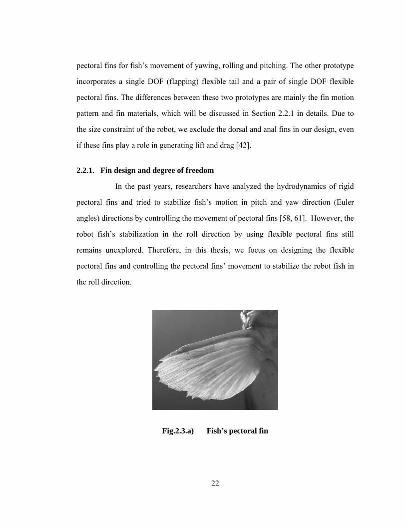
2.2.1. Fin design and degree of freedom

In the past years, researchers have analyzed the hydrodynamics of rigid

pectoral fins and tried to stabilize fish’s motion in pitch and yaw direction (Euler

angles) directions by controlling the movement of pectoral fins [58, 61]. However, the

robot fish’s stabilization in the roll direction by using flexible pectoral fins still

remains unexplored. Therefore, in this thesis, we focus on designing the flexible

pectoral fins and controlling the pectoral fins’ movement to stabilize the robot fish in

the roll direction.

Fig.2.3.a) Fish’s pectoral fin

23

Fig. 2.3 b) Pectoral fins with definition of flapping , rowing , and feathering angles

Fig. 2. 3(a) shows a pectoral fin of a boxfish in nature. The pectoral fins

have three basic moving modes: flapping, rowing, and feathering, as shown in Fig.

2.3(b). Mimicking the real fish’s pectoral fins, we designed and fabricated our flexible

fins. Fig. 2.3(b) shows the photo of an artificial fin fabricated in lab. We designed two

fish robot prototypes, which deploy different fin motion modes.

Fish prototype No. 1 has 2-DOF pectoral fins, which use both flapping and

rowing modes. The rowing DOF is employed to change the orientation of the fins at

stroke reversals [62]. Fish prototype II, however, has 1-DOF (flapping mode) pectoral

fins made of 0.003 inch thick Polyester, which makes the fins flexible in the rowing

direction. Although this type of fins only uses the flapping mode, it can also have

passive rowing motion due to its flexibility. The pectoral fins can also be effectively

24

used as lifting surfaces by holding them at a suitable angle with respect to an

oncoming flow [32, 63].

For prototype I, we use sine functions with a period of 2 seconds as the

signals to control the pectoral fins’ flapping angle and rowing angle (See Fig. 2.3.).

To mimic the pectoral fin movement of a real fish, the flapping angle and rowing

angle are controlled by two sine functions with a phase difference of 90 degrees. For

prototype II, there is only one DOF of the pectoral fins, and hence we only assign a

sine signal to control the flapping angle

Fig. 2.4 Control signals of flapping and rowing for prototype I

25

2.2.2 Mechanical chassis design

This section describes chassis of the robot fish. We design two types of

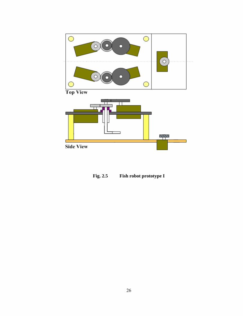
chasses for fish prototype I and prototype II, see Fig. 2.5 and 2.6. The chassis of

prototype I was made of two 0.125 inch thick Delrin plates. The upper plate is used for

mounting the servo motors and the related gearbox of the pectoral fins. The lower

plate is used for mounting the sensor board, power supply board, and motor of tail fin.

These two plates are connected by using four aluminum screws. All the parts can be

easily changed without making any modification to the chassis.

The chassis of prototype II is made of one 0.125 inch thick Delrin plate.

Three servo motors, sensor board, and power supply board are directly mounted on the

Delrin plate. The robot is carefully balanced with plastic form and aluminum screws,

which makes the mass center of the robot coincident with the center of buoyancy. All

the motors, sensors and power supply board are carefully seamed with water-proof

glue, which makes the robot be able to swim in the mineral oil/ water without

coverage of shell.

26

Fig. 2.5 Fish robot prototype I

27

Fig.2.6 Fish robot prototype II.

28

2.2.3 Actuators

A smaller robotic fish has many priorities, such as detecting small space,

less power consumption, and hard to be observed. To minimize the size of the robotic

fish, actuators with smaller sizes are necessary. In addition, for the real-time optimal

robot control, a maximum oscillating frequency of 5 Hz is needed for the mini

actuators. Accurate positioning of the fin rowing or flapping angles is required. The

actuator should also be able to generate enough force and torque for turning and

cruising. Based on these requirements, PARK HPX F Servo (GWS Inc.) motors with

built-in feedback have been selected as the actuating component in the robot fish

design, instead of DC motors and encoder combination. The PARK HPX F Servo has

small size and weight, but has relatively high speed and large torque. All the servos

are chained to a signal board fixed on the robot body. All the control signals, which

drive the servo to the right position, are transmitted from the digital ports of the NI-

DAQ board to these servos through a 16-wire cable. The servo can be controlled by

pulses with a frequency of 20Hz. The position of the servo is determined by the pulse

width. The unit of pulse width is 0.01ms. For example, when the DAQ board keeps

sending control pulses with each pulse’s duration of 1.5 ms, the servo can stay in the

neutral position. If the pulse duration changes to 2.4ms, the servo will rotate to +90

degree.

29

50ms

1.5ms

Fig. 2.7 Control pulse for servo motors

2.2.4 On board power converter

For the power concern, we built up an on-board power converter to

provide stable voltages to the motors (PARK HPX F Servo) and the sensors (ADXL

330 and IDG300). The voltages needed for the motors and the sensors are different.

The standard voltage to drive the servo motor is 5 Volts, and the standard voltage

needed by the sensors is 3 Volts. Therefore, we made two voltage-converting circuits

based on LM317 to provide two levels of voltage for the motors and the sensors. The

circuit diagram is shown in Fig. 2.7. The voltage is converted to different level by

changing the ratio of resistance 2

1

R

R . More details about the voltage converter circuit

can be found in LM317’s data manual [98].

30

22

1

1.25(1 ) , ( 50 )out Adj Adj

RV I R I A

R

Fig.2.8 LM317 and voltage converter circuit .

2.2.5 On-board Sensors

A circuit board equipped with a pair of IDG-300 dual-axis gyroscopes

(InvenSense) and one 3-axis ADXL330 accelerometer (Analog Devices) was mounted

on the robot fish. As shown in Fig 2.9, the ADXL330 is a small-sized (4 mm × 4 mm

× 1.45 mm), low-power, 3-axis accelerometer with signal conditioned voltage outputs.

It measures accelerations with a minimum full-scale range of ±3g and a sensitivity of

300mV/g. The accelerometer is used to measure the static gravity acceleration, which

is further used for estimating the attitude state of the robot fish.

The IDG-300 gyro is a small-sized (6 x 6 x 1.5mm) gyroscope, with

integrated low-pass filters. It senses the rate of rotation about two perpendicular axes

with a full scale range of ±500°/sec and a sensitivity of 2 mv/°/sec. The robot fish is

equipped with 2 pieces of IDG-300 gyro, which are mounted perpendicular to each

other in order to provide the angular rate with respect to the three axes in the body

31

reference frame of the robot. More details about the accelerometer and gyroscope

could be found in their manuals [99, 100].

Fig. 2.9 Circuit diagram of Breakout board of ADXL330 [99].

Fig. 2.10 Circuit diagram of Breakout board of IDG300 [100] .

32

2.3 Computer-based experimental platform

The computer-based experimental platform is one of the most important

parts in our experiment. The platform mainly consists of a computer equipped with

NI-DAQ driver and the Lab-view software, a PCI-6229 DAQ board, and a SCB-68

connector. This platform handles the tasks including data acquisition, signal filtering

and processing, sensor fusion, and feedback control.

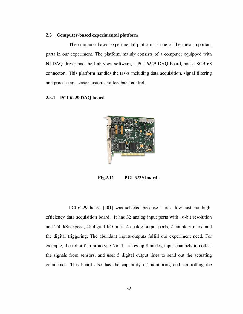
2.3.1 PCI-6229 DAQ board

Fig.2.11 PCI-6229 board .

PCI-6229 board [101] was selected because it is a low-cost but high-

efficiency data acquisition board. It has 32 analog input ports with 16-bit resolution

and 250 kS/s speed, 48 digital I/O lines, 4 analog output ports, 2 counter/timers, and

the digital triggering. The abundant inputs/outputs fulfill our experiment need. For

example, the robot fish prototype No. 1 takes up 8 analog input channels to collect

the signals from sensors, and uses 5 digital output lines to send out the actuating

commands. This board also has the capability of monitoring and controlling the

33

movement of multiple robotic fishes. More details of PCI-6229 could be found in

reference [101].

2.3.2 SCB-68 connector blocks and input/ output mode

The SCB-68 is a shielded I/O connector block with 68 screw terminals for

easy signal connection to the NI-6229 DAQ board. The open component pads allow

RC filtering easily added to the analog inputs and analog outputs.

The NI-6229 DAQ device has three input modes: single-ended-non-

reference mode (NRSE), single-ended-ground-reference (RSE) mode, and differential

(DIFF) mode. In our experiment, we connect the sensor signal to the DAQ under the

NRSE mode. The sensor signals are ground-referenced and signal-ended. The sensors

supply their own reference ground point, and the DAQ device should not supply one.

In this input mode, we connect all the signal grounds to AISENSE pin, which connects

to the negative input of the instrumentation amplifier on the DAQ device, as shown in

Fig. 2.12 [102].

Fig. 2.12 NRSE Analog input mode.

34

2.3.3 Analog input port and Digital output ports

In this experiment, we assigned different analog inputs and digital outputs

to the fish prototype No. 1 and prototype NO. 2, respectively. The assignments of

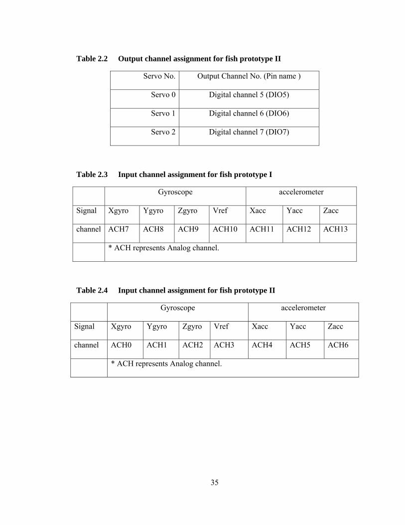
input/output channels are listed in Table 2.1 , 2.2, 2.3, and 2.4.

Fig.2.13 Servo arrangement of fish prototype I & II

Table 2.1 Output channel assignment for fish prototype I

Servo No. Output Channel No. (Pin name )

Servo 0 Digital channel 0 (DIO0)

Servo 1 Digital channel 1 (DIO1)

Servo 2 Digital channel 2 (DIO2)

Servo 3 Digital channel 3 (DIO3)

Servo 4 Digital channel 4 (DIO4)

35

Table 2.2 Output channel assignment for fish prototype II

Servo No. Output Channel No. (Pin name )

Servo 0 Digital channel 5 (DIO5)

Servo 1 Digital channel 6 (DIO6)

Servo 2 Digital channel 7 (DIO7)

Table 2.3 Input channel assignment for fish prototype I

Gyroscope accelerometer

Signal Xgyro Ygyro Zgyro Vref Xacc Yacc Zacc

channel ACH7 ACH8 ACH9 ACH10 ACH11 ACH12 ACH13

* ACH represents Analog channel.

Table 2.4 Input channel assignment for fish prototype II

Gyroscope accelerometer

Signal Xgyro Ygyro Zgyro Vref Xacc Yacc Zacc

channel ACH0 ACH1 ACH2 ACH3 ACH4 ACH5 ACH6

* ACH represents Analog channel.

36

Chapter 3

SENSOR ARRANGEMENT AND DATA COLLECTING

This chapter presents the definitions, which are directly related to attitude

estimation and stabilization of robot fish. It also describes some details which might

have significant effect on the accuracy of measurement of sensor signals. Section 3.1

present the definition of global coordinate and body fixed coordinate. In Section 3.2

the sensor alignment and calibration method are discussed.

3.1 Global coordinates and body fixed coordinates

As shown in Fig.3.1, { }G is a right orthogonal coordinate affixed to the

mini tank, such that the y-axis is parallel to the short edges of the tank and the z-axis is

pointing downwards. The body fixed frame{ }B is a right orthogonal coordinate affixed

to the robotic fish body, the origin of { }B locate in the center of buoyancy.

The robotic fish’s attitude describes the relationship between the global

coordinate frame { }G and the robot body fixed coordinate frame{ }B . Motion behavior

of the robotic fish can be described in a common way through six degree of-freedom

(DOF) in the two coordinate frames as indicated in Fig.3.1. In the global frame{ }G ,

variables , ,x y z represent the three-translation distance along three global axes, and

, , represent the three-rotation angle around the three global axes. In the body

fixed frame{ }B , variables , ,u w v describe the surge, heave and sway motion, which

are the translation velocities along the three body fixed axes, respectively, and

37

variables , ,r p q describe the rotation velocities around the three body fixed axes

respectively.

,x

,z

,y { }G

{ }B( )u surge

( )p roll

( )w heave

( )r yaw

( )q pitch

( )v sway

Fig. 3.1 Global coordinates and body fixed coordinates

According to the reference frame presented in Fig.3.1, and adopting the

yaw-pitch-roll Euler angles (ZYX), the three rotation angles are defined as (roll),

(pitch) and ψ (yaw), which are sequential rotation angles about ,b bZ Y and bX axis from

the body-fixed frame to the global frame. In this thesis, we have a micro accelerometer

and a micro gyroscope mounted in the robotic fish body, which can collect the angular

velocity about three body fixed axes and the linear acceleration along three body fixed

38

axes. This information will be used to estimate the attitude state of the robot system.

The details will be discussed in the later sections.

3.2 Sensor axis alignment, calibration and filtering

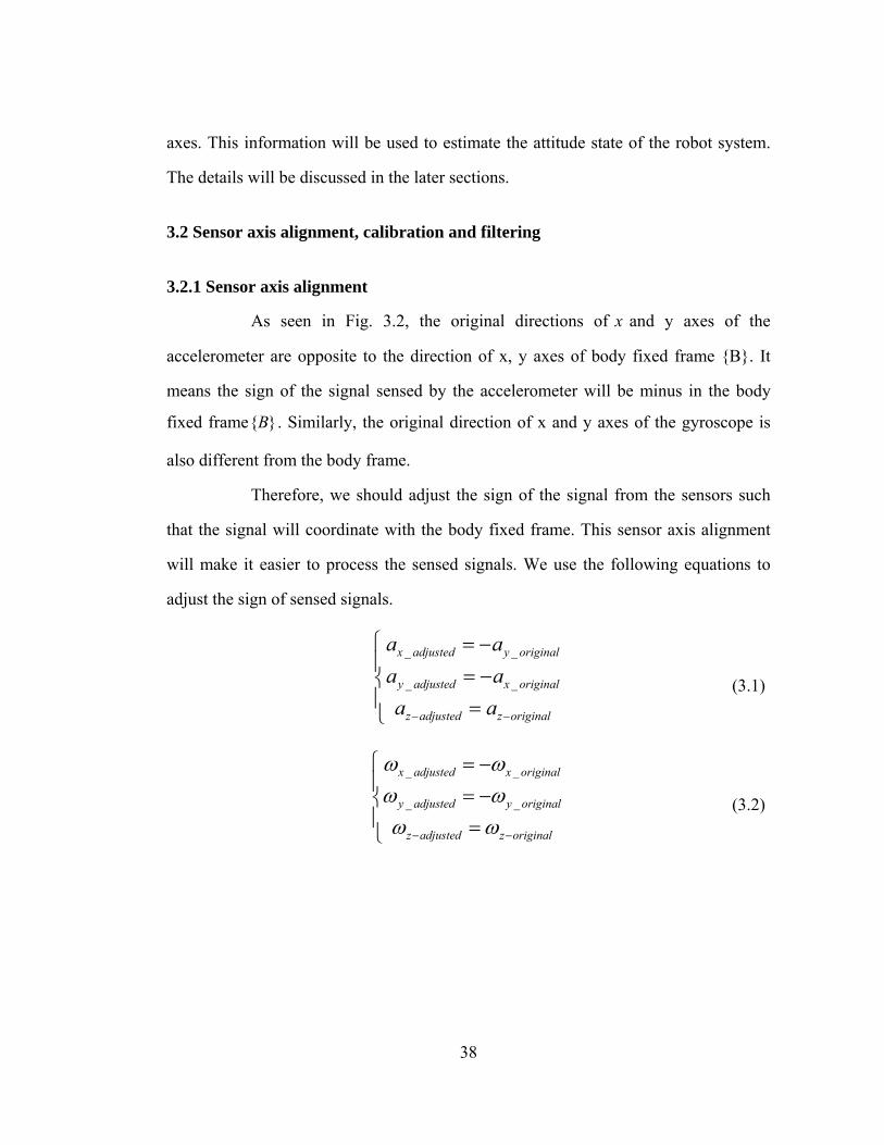
3.2.1 Sensor axis alignment

As seen in Fig. 3.2, the original directions of x and y axes of the

accelerometer are opposite to the direction of x, y axes of body fixed frame {B}. It

means the sign of the signal sensed by the accelerometer will be minus in the body

fixed frame{ }B . Similarly, the original direction of x and y axes of the gyroscope is

also different from the body frame.

Therefore, we should adjust the sign of the signal from the sensors such

that the signal will coordinate with the body fixed frame. This sensor axis alignment

will make it easier to process the sensed signals. We use the following equations to

adjust the sign of sensed signals.

_ _

_ _

x adjusted y original

y adjusted x original

z adjusted z original

a a

a a

a a

(3.1)

_ _

_ _

x adjusted x original

y adjusted y original

z adjusted z original

(3.2)

39

x

yz

{ }frame B

Fig. 3.2 Alignment of two sensors in the robotic fish.

40

3.2.2 Sensor calibration

For the accelerometer, we can easily use the gravity to finish the

calibration process. First, we can get the result of 1za g by aligning the Z axis of

the accelerometer with the direction of gravity. Then turn the accelerometer chip up-

side-down, we can get the result of 1za g by aligning the Z axis with the opposite

direction of gravity. The sensitivity of signal in axis Z can be obtained by using the

formula _ 2z z

z acc

a aSens

, and the offset of signal in axis Z can be calculated by

using the formula _ ( )z acc z zOffset a a . The calibration process for axes X and Y is

similar. Finally, the acceleration data of 3-axis can be obtained by using the following

equations:

_ _ _

_ _ _

_ _ _

( )

( )

( )

x processed x x acc x acc

y processed y y acc y acc

z processed z z acc z acc

a a offset Sens

a a offset Sens

a a offset Sens

(3.3)

The offset of gyroscope can be easily acquired by measuring the gyro’s

signal when the sensor is in static state. _z z staticOffset gyro . To obtain the

sensitivity of gyroscope, we use a 3DOF mechanical holder to assist the calibration.

As shown in Fig.3.3, the mechanical holder can generate motion in three independent

rotational degrees of freedom. The drive shafts were powered by Maxon 16mm DC

brush motors with planetary gearheads and magnetic encoders. Gearhead reductions

were 19:1 for yaw and pitch, and 84:1 for roll. The motors were driven from

MATLAB Simulink models, which used an additional toolbox provided by the control

board manufacturer (Quanser consulting) to communicate with a Q8 DAQ board. PID

41

controllers were used to run the motors at a high level of precision: up to a tenth of a

degree. Motion commands from the computer were amplified by analog amplifier

units (Advanced Motion Control) running in torque mode, which directly controls the

input current that the motor receives in order to perform a given motion.

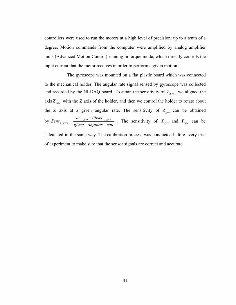
The gyroscope was mounted on a flat plastic board which was connected

to the mechanical holder. The angular rate signal sensed by gyroscope was collected

and recorded by the NI-DAQ board. To attain the sensitivity of gyroZ , we aligned the

axis gyroZ with the Z axis of the holder, and then we control the holder to rotate about

the Z axis at a given angular rate. The sensitivity of gyroZ can be obtained

by _ __ _ _

z gyro z gyroz gyro

offsetSens

given angular rate

. The sensitivity of gyroX and gyroY can be

calculated in the same way. The calibration process was conducted before every trial

of experiment to make sure that the sensor signals are correct and accurate.

42

Fig. 3.3 Three-DOF Mechanical holder [65]

3.2.3 Sensor signal acquisition and pre-processing

The signals from 3-axis accelerometer and 3-axis gyroscope were

collected by the PCI-6229 DAQ system at the same resolution (16bit) and acquisition

rate (500Hz). The full scale range of the signals of the gyroscope and accelerometer is

less than 3V and higher than 3V , therefore the programmable analog input range

of PCI-6229 DAQ was set from 3V to 3V . Since the noise mainly comes from the

disturbance of power supply, we deploy a 10Hz low-pass filter to eliminate the noise.

The whole process of data acquisition and signal filtering was conducted through the

LABVIEW program.

43

3.3 Conclusion

This chapter presents the definition of global coordinate { }G and body

fixed coordinate {B}., which are directly related to attitude estimation and

stabilization of robot fish. It also described the method of sensor alignment and

calibration, which might have significant effect on the accuracy of measurement of

sensor signals.

44

Chapter 4

SENSOR FUSION ALGORITHEM AND EXPERIMENT RESULT

In this chapter, we used two sensor fusion algorithms for estimating the

robot fish’s attitude states. The first algorithm is the Kalman filter base on Quaternion

algebra [64]. The algorithm is adapted from Trawny and Roumeliotis’s indirect

Kalman Filter for attitude estimation [64, 66]. The second sensor fusion method is a

complementary filter based on Lie algebra [65]. The detail of this algorithm can be

found in Campolo and author’s article about insect’s attitude estimate [65]. The

experiments described in this chapter validate these algorithms, especially display

some priority of the algorithm based on Lie algebra. Section 1 describes the Kalman

filter algorithm based on Quaternion algebra and presents the experiment result.

Section 2 illustrates the complementary filter based on Lie algebra and the experiment

results.

4.1 Kalman filter algorithm based on Quaternion algebra [64, 66]

4.1.1 Basic concept of Quaternion method

Quaternion is a 4-dimension vector used for describing rotation [64].

Compare with rotation matrix R which contains 9 elements, the quaternion is a

simpler representation of space rotation. The quaternion is generally defined as [66]:

1 2 3 44

1 2 3

T

T

qq q q q q

q

q q q q

(4.1)

45

The elements q1, . . . , q4 are called “quaternion of rotation” . The q4 is scalar part of

the quaternion, and q

is the vector part. Quaternion can also be written in a form [66],

in which vector k

describes the unit vector along the rotation axis and θ represent the

angle of rotation about the vector k

.

sin( ) sin( ) sin( ) cos( )

2 2 2 2

[ ]

T

x y z

x y z

q k k k

k k k k

(4.2)

The quaternion has unit norm [64, 66]:

2 2

4 1Tq q q q q

(4.3)

The quaternion multiplication is defined in matrix form as [64]:

4 3 2 1 1

3 4 1 2 2

2 1 4 3 3

1 2 3 4 4

q q q q p

q q q q pq p

q q q q p

q q q q p

(4.4)

The matrix notation q [64, 66, 68] is used to simply the quaternion multiplication.

q and the matrix form of quaternion multiplication is displayed as follow [64, 66]:

3 2

3 1

2 1

0

0

0

q q

q q q

q q

(4.5)

4 3 3

44

pq I q qq p

pq q

(4.6)

46

4.1.2 Quaternion angular velocity integral

We can estimate the rigid body’s attitude state by obtaining the instant quaternion at

any moment. If a rigid body’s angular velocity vector is constant over the

integration period 1k kt t t , then we can get the current quaternion ( )B tG q by

integrating the angular velocity using the following equation [64, 66, 67]:

1

1( ) exp( )

2 0BG k T

q t t

(4.7)

In the sensing system, the time interval has the form as: 1t f , in

which f is the data acquisition frequency of the PC-DAQ system. In this paper, the

data acquisition frequency f is equal to 1000Hz. The angular velocity can be

obtained from measurement of signal of gyroscope. Then we can use the integral

equation to calculate the quaternion, which represents the rotation from the body-fixed

coordinate to the global coordinate.

4.1.3 Translate quaternion to Rotation matrix Euler angle

Rotational matrix for transformation from global frame { }G to body fixed

frame { }B can be obtained by using the following equation [66].

2

3 3 4( ) 2 2BG R q I q q q (4.8)

According to Euler angles, , , represent rolling, pitching, and yawing about

, ,x y z axis of body fixed frame, respectively [67, 69].

, , ,( )BG z y xR q R R R

C C S C C S S S S C S C

S C C C S S S C S S S C

S C S C C

(4.9)

47

31

32

231

21

231

arcsin( ),2 2

arcsin( ),2 21

arcsin( ),2 21

r

r

r

r

r

(4.10)

4.1.4 Kalman filter for attitude estimation

The algorithm is adapted from Trawny and Roumeliotis’s indirect Kalman

Filter for attitude estimation [64, 66]. The Kalman Filter [64, 66, 67, 70, 71] contains

two stages of calculation to estimate the current attitude. In the first stage, the filter

produces an estimation of the attitude based on the integral of angular rate

measurements. In the second stage, this estimate is corrected by fusing together the

new absolute orientation measurements from field sensors (such as accelerometer,

magnetic sensor) [68, 72, 73]. Therefore, to perform a Kalman filtering, first, we

should build up the sensor measurement models in order to find the relationship

between the estimated attitude state and the real attitude state. Second, we need to

construct the estimation error state equation, so that we can get the estimation error by

solving this differentiable equation. Finally, we can update the estimated attitude state

by eliminating the error.

In this thesis, the real attitude state of a rigid body is represented by

quaternion BG q , which describes rigid body’s rotation from global frame to body fixed

frame. The estimation of attitude state is denoted by quaternion BG q , in which B denote

the estimation of the body fixed frame B . The estimation error is represented by

quaternion ˆB

Bq . The relationship between the real attitude states B

G q , the estimated

attitude BG q , and the estimation error ˆ

B

Bq is listed as follow [66, 74]:

48

ˆ

ˆB B BG GB

q q q (4.11)

Cross product aˆ 1B

G q , at both side of the Eqn. (4.11)we get [66]:

ˆ 1ˆ

ˆ 2

1

B B BG GB

B

B

q q q

(4.12)

ˆB

B

is the estimation error vector, which is the vector form for the error quaternion

ˆB

Bq .

4.1.5 Attitude estimation Stage (integrating angular rate)

Gyroscope: A three-axis gyroscope provides measurements of the

angular rate. According to reference [75, 76], we use a simple model that describes the

relationship between the measured angular rate gyro from the gyroscope and the real

angular velocity of the rotational rigid body.

gyro gyron (4.13)

In this equation, gyron

denote the measurement noise of angular rate,

which is assumed to be Gaussian white noise and [ ] 0gyroE n ,

23 3[ ]T

gyro gyro c cE n n Q I . 2

c can be found in sensor manufacture’s manual or

estimated by experiment test. To get the estimated attitude state BG q , we need to get the

integral of the angular rate measured from gyroscope and thus estimate the current

attitude state. Since the measurement from the gyroscope contains the measurement

noise gyron

, which caused the estimation error in the form of quaternion ˆB

Bq , or in the

form of vector error ˆB

B

. Thus, we need to find the state equation for the estimation

error, and then use the Kalman filter to eliminate it.

We can get the error state equation by transforming the derivative of

equation (4.11)as following [66]:

49

ˆ ˆ

ˆ ˆ

ˆ ˆ

ˆ ˆ

ˆ

ˆ ˆ

ˆ ˆ ˆ

1( )

0 02

1( )

0 02

B B B B BG G GB B

B B B B BG G GB B

gyro gyroB B B BG GB B

gyro gyroB B B

B B B

q q q q q

q q q q q

q q q q

q q q

(4.14)

By introducing Eqn(4.13), Eqn (4.12) into Eqn(4.14), the error state equation in vector

form is shown as Eqn (4.15):

ˆ ˆB B

gyro gyroB Bn

(4.15)

4.1.6 Update Stage (eliminating estimate error)

In the previous attitude estimate stage, we use the integral of angular rate

gyro from gyroscope to estimate the quaternion of rotation. We also obtain the

estimate error state equation. In this stage, we will use the accelerometer to measure

the orientation of rigid body and update the quaternion of rotation that we got in the

first stage. Therefore, we need to build up the measurement models for the

accelerometer and conduct the Kalman iterative calculation.

Accelerometer: In this model, the accelerometer obtains a projection of

gravity { }Bg

with respect to sensor frame S . The accelerometer is mounted on the

robot body, so S=equal to body fixed frame{ }B . The gravity { }Gg

in global frame

{ }G is known as a constant. The relationship between the projection of gravity in body

fixed frame { }Bg

and the gravity in global frame { }Gg

is given as follow [64]:

{ } { }( )BB G Gg R q g

(4.16)

50

Where, ( )BG R q is the rotational matrix, which represents the transformation from global

frame { }G to body fixed frame { }B . The real measurement of gravity from the

accelerometer should be represented as following [66, 77]:

{ }( )BG G accW R q g n

(4.17)

However, the estimation of gravity vector could be obtained by multiplying the

estimated rotational matrix with the constant gravity and adding the measurement

noise [66]:

ˆ

{ }ˆ ˆ( )B

G G accW R q g n

(4.18)

While, accn

is the measurement noise of accelerometer, [ ] 0accE n

and [ ]Tacc accE n n

. Let Eqn (4.17) minus Eqn (4.18), and set x

, we could get

the error between the real gravity signal and the estimation [66]:

ˆ

{ }

ˆ

{ }

ˆ

{ }

ˆ

{ }

ˆ

ˆ( ) ( )

ˆ( )

ˆ( )

ˆ( )

B BG G G acc

BG G acc

BG G acc

BG G acc

W W W

R q R q g n

R q g n

R q g n

R q g x n

(4.19)

Set matrix ˆ

{ }ˆ( )B

G GU R q g

, we obtain [66]:

accW U x n (4.20)

In addition, we can also obtain the W by using the equation

ˆ

{ }ˆ( )B

G GW W R q g , in

which W

is the measurement from accelerometer, { }Gg

is a constant, and ˆ ˆ( )B

G R q can be

calculated by Eqn(4.8).

51

Now, we relate the gravity estimation error with the attitude estimation

error vector x

, thus we obtain the state equations needed for Kalman iterative

calculation [64, 66, 67]:

gyro gyro

acc

x x n

W U x n

(4.21)

4.1.7 Kalman filter implementation

The Kalman filter is implemented in program environment LABVIEW.

We transform the continuous Kalman filter equations into the discrete-time format and

calculate the discrete-time state transition matrix and the system noise covariance

Qd [78]. The discrete-time state equations, transition matrix and the system noise

covariance Qd is shown as following [64, 66]:

23 3

23 3

( 1) ( )

ˆexp( )

k gyro

k k k acc

k

Td k gryo k

acc

x k x k n

W U x n

t

Q I t

S I

(4.22)

Given the current gravity measurement ( )W k

from the 3-axis accelerometer, and the

estimated rotation matrix ˆ( )R q , we can update our estimation of the attitude by iterate

the following steps [66, 71, 72]:

First, compute the state transition matrix k , the discrete time gyroscope

noise covariance matrix dQ , and accelerometer noise covariance matrix S , according

to Eqn (4.22).

Second, initiate the attitude estimation error vector 0x

, state covariance

matrix 0P , gravity vector { }Gg

, and the original quaternion 0q [66].

52

0 0 3 3 { } 0

00 0

00 , , 0 ,

00 1

1

Gx P I g q

(4.23)

Third, compute the current gravity measurement matrix kU , and the

residual between the real gravity kW

and estimated gravity ˆkW

[66].

ˆ

0ˆ( )B

k G accU R q a

(4.24)

ˆ

{ }ˆˆ ( ) ( )B

k G k GW W k R q g

(4.25)

Forth, compute the Kalman gain kK , and update the attitude estimation

error vector kx

.

1( )T Tk k k k k k kK P H H P H R (4.26)

1ˆˆ ˆk k k kx x K Z

(4.27)

Finally, update the quaternion 1kq , and the covariance matrix 1kP [66].

ˆkx

(4.28)

1

2q

(4.29)

2

2

2

2

1, 1

1 1

1, 1

1 1

q qq

qq

q qq

q

(4.30)

1k kq q q (4.31)

1 3 3[ ] Tk k k k k k dP I K H P Q (4.32)

53

4.1.7.1 Kalman filter experimental setup

An IDG-300 gyroscope (InvenSense) and a ADXL330 accelerometer

(Analog Devices) have been mounted on PC-controlled robotic fish (See Fig.4.1)

to mesure the angular velocity and the static gravity acceleration with respect to the

body-fixed frame (See Fig. 4.1.). The robot fish was assembled with a black shell, and

then was fixed on a metal holder (See Fig. 4.2.), which kept the robot fish free to

rotate about the x (roll) axis but limit the translation motion of the robot fish. An

MAE3 rotation encoder (See Fig. 4.3.) was mounted on the holder to measure exact

angular displacement. Since the measurement of MAE3 encoder is more accurate

result than the sensor fusion result of gyroscope and accelerometer, the output of

MAE3 encoder is viewed as the actual rotation angle of the robot fish. The sensor

fusion result is viewed as the estimated rotation angle.

The sensor data have been collected at 1 kHz sampling frequency. The

signal from accelerometer was pre-filtered by a low-pass Butterworth filter, of which

the high cut frequency is 5 Hz. The low-pass filter is used to eliminate the acceleration

caused by the robot’s vibration, since we just need the projection of static gravity in

the body fixed frame for estimating the rotation angles, any output of accelerometer

caused by other linear acceleration should be eliminated.

Both the Kalman filter program and robot fish actuation program was run

under the LABVIEW environment. The Kalman filter program is conducted offline. It

means that the program for actuating robot and collecting sensor data was run at one

time and the Kalman filter program for sensor fusion was run at another time, after the

first stage has been finished.

54

Fig. 4.1 Robot fish and the body fixed coordinate.

Fig. 4.3. Robot fish fixed on the holder.

55

Fig. 4.3 Holder and MAE3 Encoder.

4.1.7.2 Experiment results

We have conducted two different types of experiments. In the first type of

experiment, the robot fish has been passively rotated around the x axis by external

force, in the second type, the robot’s rolling motion is caused by the oscillation of

pectoral fins at 2Hz with amplitude modification. The roll angle has been derived by

performing a Kalman filter to fuse the angular velocity gyro and the gravity

projection accW

. The sensor fusion result is compared with the actual roll angle (See

Fig. 4.4. and 4.5.), which was measured with the MAE3 rotation encoder. The

comparison shows that the Kalman filter algorithm based on quaternion algebra can

precisely estimate the attitude state of the robot fish and reduce the signal noise in

certain degree.

56

4.1.8 Conclusion

Quaternion uses fewer elements than rotation matrix in representing space

rotation. The Kalman filter has been traditionally used to design attitude filters.

Therefore, the Kalman filter based on quaternion combine the advantage of quaternion

and simplifies the attitude calculating process. However, although quaternion

simplifies the calculating process, it still costs too much time to perform a Kalman

filter. This shortcoming makes the Kalman filter unsuitable for online calculation or

real-time control. In the next section, we will introduce complementary filter based on

Lie algebra, which can be used in the real-time control of robot.

Time (s)

0.4

0.2

0

-0.6

-0.2

-0.4

-0.8

-1

-1.2

0.6

0.8

0 0.5 1.0 1.5 2 2.5 2.9

EstimatedActual

ф (rad

)

Fig. 4.4 Actual and estimated roll angle (t) for movements generated by external force.

57

ф (rad

)

Fig. 4.5 Actual and estimated roll angle (t) for movements generated by fin beats.

58

Time (s)

5

0

-5

0 0.5 1.0 1.5 2 2.5 3.0 3.5 4.0 4.5 5.0

Time (s)

1

0

-1

0 0.5 1.0 1.5 2 2.5 3.0 3.5 4.0 4.5 5.0-2

2

Time (s)

0.5

0

-0.5

0 0.5 1.0 1.5 2 2.5 3.0 3.5 4.0 4.5 5.0-1

1

Fig. 4.6 Measured data from the sensors with fin flapping at 2Hz.

59

4.2 Complementary filters based on Lie algebra [65]

4.2.1 Basic definitions [65]

This section briefly describes the notations used in the complementary

filter algorithm. The details of the Lie algebra could be found in the references [65,

79-81]. The space for a rigid body is the Lie group SO (3), which is represented by a

rotation matrix R, which have traits like 1 TR R and det 1R .

Two basic coordinate frames 3S and 3

B [80]: 3S is the initial space

coordinates frame, and 3B is the body fixed frame, which is attached to the rigid

body. The rotation matrix R of SO (3) can be viewed as a map from the body frame 3B to the space frame 3

S . A trajectory of the rigid body is represented by the

curve ( )R t . The velocity vector R is tangent to the group SO(3) in R. The

TRR representing the rigid body angular velocity relative to the space frame and the

TR R representing the rigid body angular velocity relative to the body frame. There

exists a hat operator 3)3(:ˆ so [80]. For a given vector 3321 Taaaa

,

1 3 2

2 3 1

3 2 1

0

ˆ: a= 0 aˆ

0

a a a

a a a

a a a

(4.33)

Denote )3(:)( 3 so its inverse, referred to as “v” operator [80, 82]:

3 2 1

3 1 2

2 1 3

0

ˆ ˆ( ) : a 0 (a)

0

a a a

a a a

a a a

(4.34)

Moreover, the Lie brackets [·, ·] is another important operator, which defined as:

caaccaca ˆˆˆˆˆ,ˆ (4.35)

where 3, ca , a, c ∈ so(3), and × is cross product in 3 .

60

4.2.2 Complementary filter algorithm

Consider two independent and time-invariant vector ( 1v

and 2v

), which

can be expressed in any coordinate frame as:

1 2 0v v (4.36)

Define a body frame B on a given rigid body. The rigid body stays still at

the beginning 0t . Define a initial space frame 0S . Define a constant vector

0 0 0 0[ ]Ti i x i y i zv v v v

to represent the components of the space frame 0S . At time t,

define R(t) : R → SO(3) to be a twice differentiable function describing the attitude of

the rigid body with respect to the space frame 0S . [ ]Ti ix iy izv v v v would be the

components of field vector and gyro would be the readouts of the gyroscopes. The

trajectory R(t) ∈ SO(3), represent the orientation of the rigid body, can be represented

by the measurements of the gyroscopes and the vector fields sensors [82].

0

ˆ ˆTgyro

Ti i

R R

v R v

(4.37)

The * * ˆTR R denote an estimate of angular velocity, then the estimateion error[80] is:

*RRE T (4.38)

(3)( )

SOE t constant. The *( )R t denote the estimate of ( )R t , which can be obtained by

the following estimator, where 0ik are filter gains. The estimator tracks R (t) for

almost any initial condition *(0) (0)R R [80].

* * *

* *

1

* *0

ˆ

( )N

gyro i i ii

Ti i

R R

k v v

v R v

(4.39)

61

4.2.3 Numerical Implementation

The complementary filter was implemented in LABVIEW. Any digital

implementation of the filter would transform the filter into a discrete-time format with

time sequence nt and introduce numerical errors. The main risk is that numerical errors

would accumulate and quantities such as * *( )n nR R t are likely to drift away from SO

(3). The det *nR will become different from 1 and * *T

n nR R become different from the

identity matrix I. This error can be reduced by considering that sensors signal are

typically acquired via DAC (Digital to Analog Converters) with a fixed sampling time

ΔT . In the time interval Ttttt nnn 1 , data from sensors can be assumed

constantly equal to the last sampled value. Therefore, we can compute *1nR via the

Rodrigues’ formula as following[65]:

* *0

* *

2* *

* * * 2 *21

( ( ))

ˆ ˆsin /

ˆ ˆ(1 cos ) /

ˆ ˆ( )

Tn n g n b

n n n

n n n

n n n n n n

k g R g

T T

T T

R R I T T

(4.40)

Which is guaranteed not to drift away from SO(3).

4.2.4 Experimental Tests of Attitude Estimation

In this section we present the experimental results of attitude estimation

based on the complimentary filter.

4.2.4.1 Experimental Setup

A circuit board equipped with a pair of IDG-300 dual-axis gyroscopes

(InvenSense) and one 3-axis ADXL330 accelerometer (Analog Devices) was mounted

on a robot fish. The robot ws set free to rotate about the roll (x) and pitch (y) axis of

62

the metal holder (see Fig. 5). Two MAE-3 US-Digital angular sensors were

respectively mounted on the end of two rotational shafts of the holder. These MAE-3

sensors are able to measure the exact rotation angle of the robot fish about the axis x

and y. The complementary filter is used to fuse the outputs of the gyroscopes and the

accelerometer. The accelerometers are employed to measure the static gravity, while

the gyroscopes provide the angular rate with respect to the three axes in the body

reference frame.

Fig. 4.9 The holder for roll/pitch motion and the body-fixed coordinate.

63

4.2.4.2 Results

According to the reference frame presented in Fig. 5, and adopting the

yaw-pitch-roll Euler angles (ZYX), the rotation matrix R can be viewed as a map from

the body-fixed frame to the space frame given by the sequential rotation about the bZ ,

bY and bX axis[65]:

11 12 13

21 22 23

31 32 33

( ) ( ) ( )x y z

r r r

R r r r R R R

r r r

(4.41)

The , and ψ represent the roll, pitch and yaw angles, respectively. Since

this map is subjective, with the only exception of the singularity in θ = π/2 for the

pitch angle, we can directly obtain the invert Equation of , and ψ. Finally, we are

able to compare the exact rotation angel measured by the MAE3 sensors mounted on

the holder with the sensor fusion results from the complimentary filter. The inverting

Equations is listed as following:

31

32 33

21 11

arcsin( )

tan 2( , )cos( ) cos( )

tan 2( , )cos( ) cos( )

r

r ra

r ra

(4.42)

The matrix *( ) ( )TR t R t is able to converge to the identity matrix I for any

initial condition. The estimated orientation *( )R t is able to converges to the true

orientation R(t) for any initial condition of the complementary filter. In the

experiments the initial orientation *0( )R t , was set to be different from the true 0( )R t in

order to observe the speed of convergence. The results of attitude estimation from the

64

complementary filter are shown in Fig. 4.10 and the relevant sensor outputs are shown

in Fig.4.11 and 4.12.

The plots show rapid convergence of the estimated angles to the true

angles in the first half second of the experiments when the body frame is kept fixed.

The estimated angles are also able to remain very approximate the true angles during

the body motion. The effectiveness of sensor fusion could be test by removing either

the gyroscope or the accelerometers from the setup. In the first case, the removal of

the gyroscope results in an evident low pass behavior. The estimated angles include a

time lag as compared to the true angle. If the accelerometer was removed, the

estimated angles have rapid response to body motion, but there exists a drift that

overtime leads to large offset as compared to the true angles. Therefore, the

complementary filter display the capability to fuse the signals from both sensors with a

very high bandwidth [65, 84, 85].

65

Fig. 4.10 Comparison between the actual roll angle (top) and pitch angle (bottom) and three different estimations evaluated using the only accelerometers, the only gyroscopes data [97].

66

Fig. 4.11 Accelerometers output (normalized with respect to gravity g) [97]

Fig. 4.12 3-axis gyroscopes output [97]

67

Chapter 5

ATTITUDE CONTROL WITH FLEXIBLE PECTORAL FINS

This chapter presents a dynamics modeling and a linear PD controller for

robot fish’s roll control with pectoral fin. Section 5.1 describes flexible pectoral fin

design and their hydrodynamics test. Section 5.2 indicates the simplified dynamics

model of robot fish’s rolling motion with oscillating pectoral fin and the system

identification results. In section 5.3, the construction of the close-loop control system

based on a PD controller is discussed.

5.1 Flexible pectoral fin

Pectoral fin has been considered as a valuable tool for underwater

vehicle’s turning and maneuvering. In past years, researches have been conducted on

pectoral fin morphology, kinematics, hydrodynamics, and fins induced control [19,

30-33, 37, 63]. Basically, pectoral fin generates lift based thrust for propulsion by

using flapping mode, and used the rowing mode to generate a drag based thrust [19,

30-33]. In this thesis, we presented two robot fish prototypes: one equipped with a pair

of 2-DOF (flapping and rowing) pectoral fin, the other employed a pair of 1-DOF

(flapping) pectoral fin (See Fig. 5.1.). In this chapter, we mainly focus on the design of

1-DOF pectoral fin, and tests of some hydrodynamics coefficients. The design of

flexible pectoral fin focus on choosing appropriate material, fin shape, and the angle of

attack, so that the pectoral fin can produce enough force to induce or stabilize the

rolling motion of robot fish body.

68

Fig.5.1 Robot fish with 1-DOF pectoral fins.

5.1.1 Hydrodynamics forces on flapping fins

The hydrodynamics theories [86] includes incompressible and inviscid

fluid dynamics on stream lined objects, which can be used as the basis of force

production in flapping fins. The Reynolds number (Re) of a flow is defined as the ratio

of inertia force to viscous force as follows [86, 87]:

tU l

R e

(5.1)

where tU could be the forward speed of the flow or the flapping speed of the fin, l is

the characteristic length of the fin and ν is the kinematic viscosity of the fluid.

Reynolds number determines the state of the flow, and differentiates the laminar and

turbulent flow regimes [86, 87].

69

5.1.2 Lift force and drag force

A thin aerofoil is immersed in steady flow (See Fig.5.2.). The boundary

layer is attached on the solid boundary where the viscous effect is dominant [86]. At

the onset of flow, this viscosity resists the separation of flow on the foil. When the

flow leaves the trailing edge of the foil smoothly, the foil is satisfied with Kutta

condition [86]. The boundary layer is the basis of lift generation. Any steady state or

quasi steady state flow on a thin foil can be safely assumed to satisfy Kutta condition.

Pectoral fins equipped in our robot fish are assumed to satisfy the Kutta condition.

Lift force due to flow circulation

Lift force

Fig. 5.2 Steady lift generation in a two dimensional foil.

The amount of circulation needed to satisfy Kutta condition is related to

the angle of attack and the Reynolds number [86]. According to the Kutta Joukowski

theorem [86, 87], when the quasi-steady assumption is satisfied, the instantaneous

circulatory force on a flapping fin can be written as [86, 87]:

( )CF A U j (5.2)

70

where U is the total instantaneous velocity vector at the quarter chord point. Lift is

described as the vertical component of the circulatory force, which is perpendicular to

the direction of stream flow [86]. Induced drag is the horizontal component, which is

along the direction of the stream flow. By following the conventions of reference [88],

we use following equation to derive the lift and drag force [87].

21

2 F tF C U A (5.3)

where ρ is the density of fluid, Ut the path velocity of wing tip and F is the

representation of either lift (L) or drag (D). In all the experiments described in this

chapter, the area A of each fin is 24 cm2.

71

5.1.3 Fin material and angle of attack

In this thesis, our research is to study the effect of flapping flexible

pectoral fin on robot fish’s rolling motion. According to the Fig.5.3, the moment of lift

force is the mainly reason for fish’s rolling rotation; the drag force is mainly for fish’s

propulsion.

Since all of our experiments were conducted in a 60 18 16inch inch inch

mini tank, we don’t want our robot fish to generate too much drag force due to the

space limitation. In our study, we try to choose the pectoral fin which can produce

large lift force and relatively small drag force. According to Eqn. 5.3, lift force are

proportional to the coefficient LC , and the drag force are proportional to DC . Therefore,

we need to find a material with large LC and small DC to fabricate the appropriate

pectoral fin. In addition, we also need to find the suitable angle of attack for the

pectoral fin.

Rollinglift

drag

Fin foil

Angle of attack

Fig. 5.3 Forces on pectoral fin foil and angle of attack

72

In this thesis, we choose our material mainly based on the experiment

results of Zhao et al.[89]. Their experiment result shows that drag force (See Fig. 5.4.)

and lift force (See Fig.5.5) on fins of various stiffness changes as function of angle of

attack. Drag coefficient rises as angles of attack increasing (Fig.5.4.) for each flexible

fin. However, the magnitude of the drag coefficient becomes lower as the flexibility of

fin increasing. Thus, the ability of a flexible fin to generate drag decreases with

increasing flexibility. Similarly, lift coefficients also decrease in magnitude as fin

flexibility increases, but plateau at higher angles of attack [89]. At angles of attack

greater than 60o, flexible fins generate more lift than rigid fins. An important point is

that Zhao’s experiment results shows that a very flexible fin moving at 90 degree

angle of attack can still generate certain lift while not generating as much drag as a

rigid plate. Therefore, we can use flexible pectoral fin moving at 90 degree angle of

attack to generate large lift force for rolling control, and less drag in propulsion. Since

our experiment environment is almost the same with that of Zhao’s group (The

mineral oil used for our robot experiment is the same with that used in Zhao’s group

and the dimension of our fin is also very close to the dimension of wings in Zhao’s

experiment.), we adopt their experiment result as the basic rules for choosing our

materials of fins. Finally, we choose polyester sheet of 0.003 inch thickness to make

our flexible pectoral fin. The pectoral fin’s angle of attack was set at 90 degree.

73

Fig.5.4 a) Drag coefficient of flexible foil as function of angle of attack [89].

Fig.5.4 b) Lift coefficient of flexible foil as function of angle of attack [89]

74

5.1.4 Pectoral fin shape design.

We conduct a preliminary study about the effect of fin shape on the robot

fish’s rolling motion. In our study, the principle for choosing a fin shape is to generate

the maximum rotational angle in roll direction, when only one pectoral fin was

actuated. . Three fin shapes: rectangular, triangle, a bluegill sunfish like fin as shown

in Fig. 5.5 is used. The material used for fabricating the fins was a 0.003 inch thick

polyster sheet. The dimensions of the fin were found by fixing the area to be 24 cm2

and the length of fin to be 6cm. The fin was driven in a 1-degree of freedom sine-wave

motion * sin(2 )ft . The flapping frequency f was set at 3Hz, and the amplitude

* of flapping is set at 30 degree, the angle of attack is 90 degree. Renold number for

the experiments was in the range of 2000.

For the experiment setup, there is a cylindrical connector (Fig. 5.5.) fixed

on the rotational shaft of the servo motor. Three different types of fins were attached

to the cylindrical connector respectively by tightening the screw. By using this

cylindrical connector, we can change the fin shape and set up the pectoral fin’s angle

of attack easily.

Three experiments were done to compare the effect of fin shape on the

robot fish’s rotation. In each experiment, a pair of pectoral fin with specific shape was

attached to the robot fish, which was then assembled with a black shell and attached to

a mechanical holder. The holder limit the translational movement of the robot fish,

only permit the robot fish to rotate in the roll direction. (See Fig.5.6.). During each

experiment, only one fin (left or right) was driven under the sine-wave function. The

robot fish’s rolling angle was measured by the MAE3 rotation encoder. Each fin shape

was tested twice (left fin and right fin). Finally, the measured rolling angles were

75

compared between these different fin shapes setting. The rectangular fin shape, which

can induce largest rolling angle of the robot fish, was chosen as the final fin shape.

Servo motor

Screw

Rotation shaft

Fig.5.5 Three kinds of fin shape and the cylindrical connector.

76

Fig.5.6 The robot fish with holder and sensors.

5.2 Roll plane dynamics of robotic fish

In this thesis, a robot fish has been built to study fish swimming dynamics

in roll direction with the flapping pectoral fin.

5.2.1 Simplified moment equation

The robot is equipped with a 3-axis accelerometer and a 3-axis gyroscope

to measure the rotation angle about roll direction. To simplify the dynamics analysis,

the robot fish was fixed on a mechanical holder (See Fig.5.6), which limit the

translational movement of robot fish, and only allows 1 degree of freedom rotation in

the roll direction. With this simplified setting, we can neglect the drag terms, and the

buoyancy terms, only take the lift force into consideration. In addition, we also neglect

the friction force of the bearing, and assume the roll rotation to be perfect. Therefore,

77

the rolling equation of a 1-DOF robot fish with respect to the body fixed frame can be

written as following:

0bxF (5.4)

b bx xI k M (5.5)

where is the rotation angle about bx axis, bxM is the roll moment due to the lift

force induced by flapping pectoral fins. bxI is the moment of inertia about the bx axis.

The parameter k denotes the effects of the lift in the roll dynamics.

Since the external roll moment bxM is due to the lift force induced by

oscillating pectoral fins, we can write the roll moment bxM as follows:

( )x left rightM F F d (5.6)

Where, leftFand rightF

are the lift force induced by the left and right pectoral fin,

respectively. The parameter d is the perpendicular distance from the force center of

pectoral fin to the center of mass of fish body. According to hydrodynamics literature

[41, 86, 87, 89], the lift force induced by a pair of oscillating pectoral fin can be

obtained by using the following equation.

2

2

1

21

2

Left LL Left L

right LR right R

F C U A

F C U A

(5.7)

where ρ is the density of fluid, LeftUand rightU

is the path velocity of force center on

pectoral left and right pectoral fin respectively. LA and RA is the area of the left fin and

right fin respectively. We assume that the left and the right pectoral fin are identical

( L RA A ) and are oscillating at a fixed frequency and angle of attack, so the lift

78

coefficients for the left and right fin are equal to each other. ( LL LR LC C C

Constant). Take the Eqn. (5.7) into Eqn.(5.6), we obtain the equation for moment as

following:

2 21

( )2x lift left rightM AC d U U (5.8)

The left and right pectoral fins are oscillating with the same period T (oscillating

frequency1

fT

), we can derive the moment as follows:

2 2

0

2 2

0

1( )

2

1( )

2

T

x lift left right

T

lift left right

M AC d U U dt

AC d U U dt

(5.9)

Path velocity of LeftU and rightU are related to the oscillating angle of pectoral fins.

( ) ( )

( ) ( )

left left

right right

U t t l

U t t l

(5.10)

Where, the left and ( )right t are the oscillating angular velocity of left and right

pectoral fins, and l is the distance from the center of force to the base of the fin. To

obtain the dynamic relationship between the roll angle and the oscillation of pectoral

fins, we need to define the control variable of pectoral fins.

5.2.2 Control variable of pectoral fins

As describe in previous chapter 2, the 1-DOF pectoral fins of the robot

fish are driven in a sine-wave function as follows:

( ) sin(2 ) 1,2i i i i it A f t i (5.11)

79

Where, i is the oscillating angle of pectoral fin, iA is the magnitude of the fin

oscillating, if is the oscillating frequency, i is the phase, and i is the offset of the fin

oscillating, which determine the neutral position of pectoral fin. The definition of

oscillating angle of pectoral fins is shown in Fig. 5.7.

Fig. 5.7 Definition of oscillating angle of pectoral fin.

For this robot fish, all of these parameters iA , if , i , and i could be used as

control variables. Base on observation of fish swimming kinematics, we choose iA as

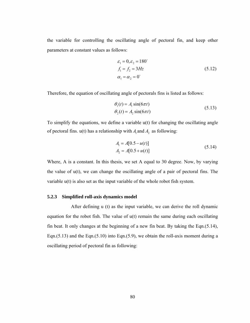
80

the variable for controlling the oscillating angle of pectoral fin, and keep other

parameters at constant values as follows:

1 2

1 2

1 2

0, 180

3

0

f f Hz

(5.12)

Therefore, the equation of oscillating angle of pectorals fins is listed as follows:

1 1

2 2

( ) sin(6 )

( ) sin(6 )

t A t

t A t

(5.13)

To simplify the equations, we define a variable u(t) for changing the oscillating angle

of pectoral fins. u(t) has a relationship with 1A and 2A as following:

1

2

[0.5 ( )]

[0.5 ( )]

A A u t

A A u t

(5.14)

Where, A is a constant. In this thesis, we set A equal to 30 degree. Now, by varying

the value of u(t), we can change the oscillating angle of a pair of pectoral fins. The

variable u(t) is also set as the input variable of the whole robot fish system.

5.2.3 Simplified roll-axis dynamics model

After defining u (t) as the input variable, we can derive the roll dynamic

equation for the robot fish. The value of u(t) remain the same during each oscillating

fin beat. It only changes at the beginning of a new fin beat. By taking the Eqn.(5.14),

Eqn.(5.13) and the Eqn.(5.10) into Eqn.(5.9), we obtain the roll-axis moment during a

oscillating period of pectoral fin as following:

81

2 2 2 2 2

0

2 2 2 2 2

0

1( ) ((0.5 ) cos (2 ) (0.5 ) cos (2 ))

2

2 cos (2 )

u

T

x lift

T

lift

K

u

M AC d l f u ft u ft dt

u AC dl f ft dt

K u

(5.15)

Where, uK is a constant. Take the Eqn.(5.15) into Eqn. (5.5), we can get the

simplified dynamics model to represent the relationship between robot fish’s roll-axis

rotation angle ( )t and the oscillating variable u(t) of pectoral fin.

( ) ( ) ( )x uI t k t k u t (5.16)

Then, we get the transfer function, in which the rotational angle ( )s about roll axis

is the output and the magnitude variable ( )U s of oscillating angle of pectoral fin is the

input.

2 ( ) ( ) ( )

( )( ) ( )

x u

u

x

s I s sk s K U s

KsU s s I s k

(5.17)

Base on this dynamics equation, we can use the LABVIEW system identification

module to find the optimal value of xI , k , and uK and build up the final dynamics

model of robot fish’s roll rotation.

5.2.3 System model identification

The goal of model identification process is to obtain the optimal value of xI ,k , and

uK for Eqn.(5.17), and then to build up the open-loop dynamics model that match the

experiment data well. For the fixed robot fish, the system model is a transfer function,

which relates the variable u(t) of oscillating angle of pectoral fin with the robot fish’s

82

rolling angle ( )t . Based on Eqn. (5.17), we know that the direct transfer function of

the robot fish is a second order system with a integral component. Hence, we just need

to identify the transfer function between input u(t) and angular velocity

( ) ( )t t about roll axis and find the optimal value for xI ,k , and uK as follows:

( )( )

u

x

KsU s I s k

(5.18)

In the identification experiments, the robot fish was fixed on the holder

(See Fig.5.6.) and immersed in a mini tank (46 cm width, 41 cm height, and 152 cm

length) filled with mineral oil (Kinematic viscosity= 3.4 cSt at 20o C, density=850

kg/m3). The pair of pectoral fins was driven by sine-wave functions, with the

parameters setting as Eqn.(5.12). The input variable ( )u t uses a white noise signal

with 2( ) 0, { ( ) } 0.3E u t E u t . The roll angle ( )t and the angular velocity ( )t were

estimated from signals of accelerometer and gyroscope on the robot body by using the

complementary filter based on Lie group (See Chapter 4.2).

The time interval T of the control variable u(t) is 0.02 sec. After every

experiment, the input data u(t) and the output data roll angle ( )t and the angular

velocity ( )t were recorded and separated into two parts with equal length. The first

part of data is used for system identification processing; the other part is used for

validating the acquired model. In addition, before starting the identification iteration,

all the data (input and output signals) were pre-filtered and removed the trend by using

the pre-processing module in LABVIEW.

The system identification iteration based on zero-order-hold method, is

easily done by using discrete transfer function estimation module in LABVIEW. After

83

the several trials of identification iteration, we obtained the model equation relating

input u(t) and angular velocity ( )t as follows:

21.001( )

( ) ( 1.923)s

U s s

(5.19)

Based on Eqn.(5.19), we can obtain the transfer function between input variable u(t)

and the rotational angle ( )t about roll axis, as follows:

21.001( )

( ) ( 1.923)s

U s s s

(5.20)

Fig.5.8 a) Validating result of ( )( )

sU s

by using white noise input.

84

Fig.5.8 b) Validating results of ( )( )

sU s

by using sine-wave input

The model described in Eqn(5.19) was validated by using robot fish

rolling motion experiments. The Fig. 5.8 a) shows the validating result of ( )

( )s

U s by using the white noise input and the corresponding output. The Fig.5.8 b)

shows the validating result of ( )( )

sU s

by using the sine-wave input and the

corresponding output. The Fig.5.8 c) shows the validating result of ( )( )

sU s

by using

the sine-wave input and the output.

85

Fig.5.8 c) Validating results of ( )( )

sU s

by using sine-wave input.

The validating result shows that this roll-axis dynamics model acquired by

using identification iteration matches the experiment data well. Hence, this model can

be used in the PD controller design, which is described in the next section.

5.3 PD Controller design for robot fish fixed on holder

In this section, we design a PD (Proportional Derivative) controller [83,

90] for the robot fish fixed on the holder. The schematic of the control system is

shown in Fig. 5.9.

86

OPGservoGcontrollerG

sensorG

R(s) Φ(s)

D(s)

Fig.5.9 Schematic of control system of robot fish

In this schematic, the rotation angle ( )s is the control output, ( )R s is the

reference input (assigned rotation angle), and ( )D s is an external disturbance.

Therefore, the close-loop transfer function is shown as following [83, 90]:

( )( ) 1

controller servo op

controller servo op sensor

G G GsR s G G G G

(5.21)

( )( ) 1

op

controller servo op sensor

GD sR s G G G G

(5.22)

Where, 21.001

( 1.923)opGs s

is the open-loop transfer function of the robot fish,

and controllerG , servoG and sensorG are the transfer functions of controller, servo and sensor

respectively. By designing a PD controller for the robot, we try to varying robot fish’s

rotation angle according to the assigned trajectory.

In this thesis, the Bode plot method [83, 91-95] was used to design the PD

controller. We assume that the response speed of servo motor is large enough, thus we

get 1servoG . Similarly, we also assume the sampling time of sensor is negligible,

thus 1sensorG .

87

( )( ) 1

( )( ) 1

controller op

controller op

op

controller op

G GsR s G G

GD sR s G G

(5.23)

We design a PD controller (with inertia component) with parameter T and . The

transfer function of PD controller [91-93, 95] is shown as Eqn.(5.24).

1

2

11

1( )

11 1controller

ss

G sTs s

(5.24)

We make the ( 1)bT b , then the transfer function of the PD controller is listed as

following [91-93, 95]:

1

2

11

1( )

11 1controller

sbTs

G sTs s

(5.25)

We have known that the open-loop transfer function of the robot system

is21.001

( 1.923)opGs s

, thus we can plot its Bode diagram as shown in Fig. 5.10. The

crossover frequency of the open-loop system is shown as following [91-93, 95]:

4 2_ 1 4 2 4.38 /c op n rad s (5.26)

In addition, the phase margin of the open-loop system

is4 2

arctan 12.41 4 2

, and the adjusting time3.5

3.64secsn

t

.Thus,

we use the PD controller to enlarge the phase margin in order to improve the stability

of the system. The phase margin of the controlled close-loop system is set as 45 .

88

By using the Bode plot method, we choose 1 3.5 /rad s (the

corresponding point in the line of 20lg opG is point A), and then we made a straight

line with slope of -20db/dec across the point A and the 0db line. Then, we can get the

crossover frequency of the controlled close-loop system [91-93, 95]

5.26 /c controlled rad s .

Finally, we can get the value of 2 by using the equation as follow: 2 2

21

5.267.9 /

3.5c controlled rad s

.

Therefore, with the values of 1 and 2 , we obtain the transfer function of the

controller:

1 0.286

1 0.126controller

sG

s

(5.27)

The phase margin of the controlled system is shown as follow:

4 2arctan 45.93

1 4 2controlled

Finally, the transfer function of the controlled system is shown as follow:

20.001(1 0.286 )( )

( ) (1 0.126 )(1 1.923 )

ssR s s s s

(5.28)

89

0db1.923

Glg20

4.381 c 2

A

20lg|G |OP

20lg| G |controlled

20lg| G |controller

Fig.5.10 Bode plot of frequency response of open-loop system, close-loop system and the controller.

Based on this PD controller, the experiment result of roll angle control of

the robot fish (fixed on the holder) is obtained and shown in Fig.5.11 a), Fig.5.11 b),

and Fig.5.12.

90

Fig.5.11a) The roll angle stabilized at 180 degree.

Fig.5.11b) The control variable u(t) used to stabilize the roll angle at 180 degree

91

Fig.5.12 The roll angle of robot fish (with holder) tracking a sine-wave

5.4 PD controller for rolling angle tracking of free robot fish

The PD controller designed in section 5.3 was also used in the rolling

angle control of robot fish without the mechanical holder. Although the motion about

yaw axis and pitch axis are not regulated in the free robot fish, the experiment results

of roll angle control are still acceptable. The experiments results are shown in the

following pictures.

92

Fig.13a) The roll angle of robot fish stabilized at 20 degree.

93

Fig.13b) The roll angle of robot fish stabilized at 0 degree.

Fig.13c) Roll angle of robot fish tracking a sine-wave with magnitude of 45 degree

94

Fig.13d) Roll angle of robot fish tracking a sine-wave with magnitude of 75 degree

5.5 Conclusion

This chapter mainly describes the system dynamics modeling and the

linear PD controller design for the robot fish with oscillating pectoral fin. It also

presents the flexible pectoral fin design by choosing appropriate material and fin shape.

Although the simplified model of the robot fish and the linearized PD controller can

get acceptable results in the roll angle control, the neglected nonlinear term is still

remain unregulated. To make the robot fish track the pre-assigned trajectory more

accurately, more complex dynamics model should be derived and more efficient

controller for multi-degree of freedom stabilization should be developed in future

study.

95

Chapter 6

CONCLUSIONS AND FUTURE WORK

This thesis presents the development of a small size robot fish which is

equipped with flexible pectoral fins and attitude measurement sensors. The thesis also

presents a new idea in controlling robot fish’s roll plane maneuvering using a pair of

flexible pectoral fins. The one degree of freedom (1DOF) flexible pectoral fins were

driven by mini servos to mimic real fish’s fin motion, and the experiment results

validate the function of flexible pectoral fin in stabilizing robot fish’s rolling motion.

Many researchers have used mechanical pectoral fins to stabilize the movements of an

autonomous underwater vehicle. These mechanical pectoral fins were usually made

from rigid foils [1, 60], the pectoral fin made from flexible materials was barely used.

In addition, the dive and yaw plane motion control is the focus of previous researches,

using computational fluid dynamics (CFD) method or real experiment [58, 96]. This

thesis presents the roll plane maneuvering control using oscillating flexible pectoral is

relatively new when compared with other similar researches in this field.

In addition, two sensor fusion methods (Kalman filter based on quaternion

and Complementary filter based on Lie groups) were used to estimate robot fish’s

attitude state. The complementary filter based on Lie groups is a new attitude fusion

method, which was presented in Campolo* and author’s article [65, 97]. The

experiment results presented in chapter 4 validated this algorithm. Moreover, the robot

fish’s roll motion dynamics model was analyzed, and a linear feedback controller was

96

designed based on this dynamics model. Following sections summarize the findings

and describe some near future extensions of this work.

6.1 Summary of the work presented

6.1.1 Robotic Prototype and flexible pectoral fin design

Two robotic prototype of the MUV was designed based on mimicking

some characteristic of real fish. The difference between these two robot fish prototype

is the degree of freedom (DOF) of pectoral fins. In this thesis, the robot fish with a

pair of 1DOF pectoral fins is the mainly research object. The propulsion and

maneuvering of the MUV is achieved by flapping flexible pectoral fins.

The robot consists of a chassis that holds the flapping fin mechanisms for

the pectoral and tail and fins. The power supply electronics and two sensors (a 3-axis

accelerometer and a 3-axis gyroscope) are mounted on the robot. These electronics

and sensor are used to collecting signal which can be used for estimating the attitude

of the robot fish. Collecting of sensor signals and sending control command was

accomplished by computer and PCI-6229 DAQ board. All the sensor fusion and

control experiments were conducted based on this robot fish and its computer system.

The flexible pectoral fins were made from material, which are chosen

depending on their coefficient of lift. The fin shape was selected by a series of robot

fish experiments.

97

6.1.2 Sensor fusion for attitude estimation

In this thesis, we used two sensor fusion algorithms for estimating the

robot fish’s attitude states. The first algorithm is the traditional Kalman filter base on

Quaternion algebra, the second one is a complementary filter based on Lie algebra.

Our experiments results validate these algorithms. Especially, the complementary

filter based on Lie group display some priority over the Kalmann filter based on

quaternion algebra. Running the Kalman filter algorithm used in this thesis is time

consuming. This shortcoming makes the Kalman filter unsuitable for online

calculation or real-time control. The complementary filter based on Lie algebra has

high accuracy and small amount of calculation, and thus it can be used in the real-time

control of robot.

6.1.3 Roll motion dynamics modeling and linear control

We analyzed the dynamics model of robot fish’s rolling motion under

flapping pectoral fin, and construct a linear PD controller for roll plane control. The

dynamics model was built up based on a series of simplifying assumptions, including

neglecting the drag terms, the buoyancy terms, and the friction term. The system

identification process has been conducted in the LABVIEW test environment. A linear

PD controller based on the simplified model and the system identification result was

designed by using the Bode plot method. The simplified model and controller got

good result in rolling motion experiments. The linear PD control is based on the feed

back attitude, which is estimated from the outputs of gyroscope and accelerometer by

using Kalman filter or Complementary filter.

98

6.2 Future Work

6.2.1 3-DOF flexible pectoral fin

The idea is to build up an upgraded robot fish prototype with 3-DOF

flexible pectoral fins. By carefully design the 3-DOF fin motion, we could mimic the

real fish’s fin movement better than 1-DOF fin. In addition, by using 3-DOF pectoral

fins, we would be able to control the robot fish’s maneuvering in 6-degree of freedom,

which is hard to achieve with 1-DOF pectoral fins. Moreover, flexible material might

play a more important role in 3-DOF pectoral fin motion.

6.2.2 Wireless signal transmit and more sensors

In this thesis, collecting sensor signal and sending control command was

transmitted through a 16-wire cable. Although these wires are very thin and light,

they still cause noise to sensors and introduce disturbances to the control system.

Therefore, the next step to upgrade the robot fish is to transmit all signals by wireless

method. This method will reduce the noise and uncertainty of the control system, and

make the control more efficient and accurate.

Moreover, to estimate more accurate attitude state, we need more

orientation sensors. Although the Kalman filter and complementary filter in this thesis

can fuse the signals from accelerometer and gyroscope together, there is still some

noise, especially the dynamic drift, contained in the estimation of attitude. To reduce

this noises more orientation vector sensors need to be added into this robot system.

6.2.3 Fin-fin interaction and complex control

Conducting research about fin-fin interactions can help modify fin

kinematics for optimal lift production or even better maneuverability. In this thesis,

99

the robot fish is controlled in one degree of freedom by a pair of pectoral fins, actually

the pectoral fins need to work with tail fin to reach better maneuverability for real fish.

Therefore, in future work, the interactions between the pectoral fin and tail fin need to

be analyzed to get higher performance in propulsion and maneuvering. The

introduction of fin interaction might lead to more complex dynamics model and

control method. Except the PD control method used in this thesis, the inverse control

is another widely used control law in regulating fish’s motion [4]. Our linear attitude

control research in the roll plane provides the base for future complex control.

100

Appendix A

SAMPLE CODE OF KALMAN FILTER AND PD CONTROL IN LABVIEW

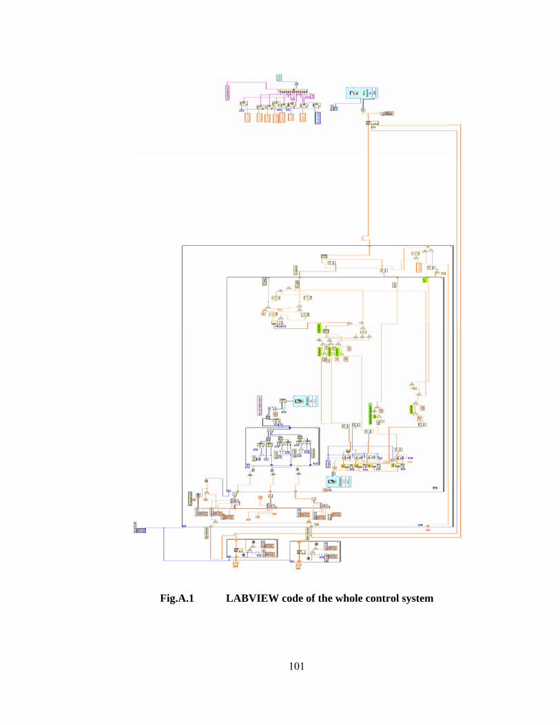
101

Fig.A.1 LABVIEW code of the whole control system

102

Fig. A.2 LABVIEW code of Kalman filter

103

Appendix B

SOFTWARE USER INTERFACE

Fig.B.1 LABVIEW Interface for control system

104

Reference

1. Licht, S., Design and projected performance of a flapping foil AUV. IEEE Journal of Oceanic Engineering, 2004. 29(3): p. 786-794.

2. Lauder, G.V. and E.G. Drucker, Morphology and experimental hydrodynamics of fish fin control surfaces. IEEE Journal of Oceanic Engineering, 2004. 29(3): p. 556-571.

3. Bandyopadhyay, P.R., Maneuvering hydrodynamics of fish and small underwater vehicles. Integrative and Comparative Biology, 2002. 42(1): p. 102-117.

4. Singh, S.N., A. Simha, and R. Mittal, Biorobotic AUV maneuvering by pectoral fins: Inverse control design based on CFD parameterization. IEEE Journal of Oceanic Engineering, 2004. 29(3): p. 777-785.

5. Cristi, R., F.A. Papoulias, and A.J. Healey, Adaptive Sliding Mode Control of Autonomous Underwater Vehicles in the Dive Plane. IEEE Journal of Oceanic Engineering, 1990. 15(3): p. 152-160.

6. Narasimhan, M. and S.N. Singh, Adaptive optimal control of an autonomous underwater vehicle in the dive plane using dorsal fins. Ocean Engineering, 2006. 33(3-4): p. 404-416.

7. Narasimhan, M. and S.N. Singh, Adaptive input-output feedback linearizing yaw plane control of BAUV using dorsal fins. Ocean Engineering, 2006. 33(11-12): p. 1413-1430.

8. Wong, H., V. Kapila, and A.G. Sparks, Adaptive output feedback tracking control of spacecraft formation. International Journal of Robust and Nonlinear Control, 2002. 12(2-3): p. 117-139.

9. Sfakiotakis, M., D.M. Lane, and J.B.C. Davies, Review of fish swimming modes for aquatic locomotion. IEEE Journal of Oceanic Engineering, 1999. 24(2): p. 237-252.

10. Breder, C.M., Respiration as a factor in locomotion of fishes. American Naturalist, 1924. 58: p. 145-155.

105

11. Wilga, C.D. and G.V. Lauder, Function of the pectoral fins during locomotion in the bamboo shark Chiloscyllium plagiosum. American Zoologist, 1999. 39(5): p. 55a-55a.

12. Lauder, G.V., Function of the caudal fin during locomotion in fishes: Kinematics, flow visualization, and evolutionary patterns. American Zoologist, 2000. 40(1): p. 101-122.

13. Drucker, E.G. and G.V. Lauder, Function of pectoral fins in rainbow trout: behavioral repertoire and hydrodynamic forces. Journal of Experimental Biology, 2003. 206(5): p. 813-826.

14. Thorsen, D.H., M.H. Green, and M.E. Hale, Motor control of the zebraffsh pectoral fin. Integrative and Comparative Biology, 2006. 46: p. E257-E257.

15. Fiorelli, E., N. E. Leonard, P. Bhatta, D. A. Paley, R. Bachmayer, and D. M. Fratantoni, Multi-AUV control and adaptive sampling in Monterey Bay. IEEE Journal of Oceanic Engineering, 2006. 31(4): p. 935-948.

16. Wilga, C.D. and G.V. Lauder, Locomotion in sturgeon: Function of the pectoral fins. Journal of Experimental Biology, 1999. 202(18): p. 2413-2432.

17. Colgate, J.E. and K.M. Lynch, Mechanics and control of swimming: A review. IEEE Journal of Oceanic Engineering, 2004. 29(3): p. 660-673.

18. Kodati, P., J. Hinkle, A. Winn, and X. Y. Deng, Microautonomous robotic ostraciiform (MARCO): Hydrodynamics, design, and fabrication. IEEE Transactions on Robotics, 2008. 24(1): p. 105-117.

19. Kato, N., Control performance in the horizontal plane of a fish robot with mechanical pectoral fins. IEEE Journal of Oceanic Engineering, 2000. 25(1): p. 121-129.

20. Bandyopadhyay, P.R., Trends in biorobotic autonomous undersea vehicles. IEEE Journal of Oceanic Engineering, 2005. 30(1): p. 109-139.

21. Triantafyllou, M.S. and G.S. Triantafyllou, An Efficient Swimming Machine. Scientific American, 1995. 272(3): p. 64-70.

22. Triantafyllou, M.S., A.H. Techet, and F.S. Hover, Review of experimental work in biomimetic foils. IEEE Journal of Oceanic Engineering, 2004. 29(3): p. 585-594.

106

23. Triantafyllou, M.S., A. H. Techet, Q. Zhu, D. N. Beal, F. S. Hover, and D. K. P. Yue, Vorticity control in fish-like propulsion and maneuvering. Integrative and Comparative Biology, 2002. 42(5): p. 1026-1031.

24. Barrett, D.S., M. S. Triantafyllou, D. K. P. Yue, M. A. Grosenbaugh, and M. J. Wolfgang, Drag reduction in fish-like locomotion. Journal of Fluid Mechanics, 1999. 392: p. 183-212.

25. Williamson, C.H.K. and R. Govardhan, Vortex-induced vibrations. Annual Review of Fluid Mechanics, 2004. 36: p. 413-455.

26. Triantafyllou, M.S., G.S. Triantafyllou, and R. Gopalkrishnan, Wake Mechanics for Thrust Generation in Oscillating Foils. Physics of Fluids a-Fluid Dynamics, 1991. 3(12): p. 2835-2837.

27. Drucker, E.G. and G.V. Lauder, Wake dynamics and locomotor function in fishes: Interpreting evolutionary patterns in pectoral fin design. Integrative and Comparative Biology, 2002. 42(5): p. 997-1008.

28. Read, D.A., F.S. Hover, and M.S. Triantafyllou, Forces on oscillating foils for propulsion and maneuvering. Journal of Fluids and Structures, 2003. 17(1): p. 163-183.

29. Saimek, S. and P.Y. Li, Motion planning and control of a swimming machine. International Journal of Robotics Research, 2004. 23(1): p. 27-53.

30. Hale, M.E., R. D. Day, D. H. Thorsen, and M. W. Westneat, Pectoral fin coordination and gait transitions in steadily swimming juvenile reef fishes. Journal of Experimental Biology, 2006. 209(19): p. 3708-3718.

31. Lauder, G.V. and B.C. Jayne, Pectoral fin locomotion in fishes: Testing drag-based models using three-dimensional kinematics. American Zoologist, 1996. 36(6): p. 567-581.

32. Drucker, E.G. and J.S. Jensen, Pectoral fin locomotion in the striped surfperch .1. Kinematic effects of swimming speed and body size. Journal of Experimental Biology, 1996. 199(10): p. 2235-2242.

33. Drucker, E.G. and J.S. Jensen, Pectoral fin locomotion in the striped surfperch .2. Scaling swimming kinematics and performance at a gait transition. Journal of Experimental Biology, 1996. 199(10): p. 2243-2252.

107

34. McIsaac, K.A. and J.P. Ostrowski, Motion planning for anguilliform locomotion. IEEE Transactions on Robotics and Automation, 2003. 19(4): p. 637-652.

35. Westneat, M.W., D. H. Thorsen, J. A. Walker, and M. E. Hale, Structure, function, and neural control of pectoral fins in fishes. IEEE Journal of Oceanic Engineering, 2004. 29(3): p. 674-683.

36. Yamamoto, I., Y. Terada, T. Nagamatu, and Y. Imaizumi, Propulsion System with Flexible Rigid Oscillating Fin. IEEE Journal of Oceanic Engineering, 1995. 20(1): p. 23-30.

37. Kato, N. and H. Liu, Optimization of motion of a mechanical pectoral fin. Jsme International Journal Series C-Mechanical Systems Machine Elements and Manufacturing, 2003. 46(4): p. 1356-1362.

38. Tytell, E.D. and G.V. Lauder, Kinematics and wake structure of steadily swimming eels (Anguilla rostrata). Integrative and Comparative Biology, 2002. 42(6): p. 1326-1326.

39. Walker, J.A. and M.W. Westneat, Kinematics, dynamics, and energetics of rowing and flapping propulsion in fishes. Integrative and Comparative Biology, 2002. 42(5): p. 1032-1043.

40. Walker, J.A., M. W. Westneat, W. C. Sandberg, R. Ramamurti, and L. Rosenberger, Kinematics, dynamics, energetics, performance, and ecomorphology of rowing and flapping propulsion. American Zoologist, 2001. 41(6): p. 1618-1619.

41. Kato, N., Hydrodynamic characteristics of a mechanical pectoral fin. Journal of Fluids Engineering-Transactions of the Asme, 1999. 121(3): p. 605-613.

42. Zhu, Q., Three-dimensional flow structures and vorticity control in fish-like swimming. Journal of Fluid Mechanics, 2002. 468: p. 1-28.

43. Webb, P.W., Kinematics of Pectoral Fin Propulsion in Cymatogaster-Aggregata. Journal of Experimental Biology, 1973. 59(3): p. 697-710.

44. Bandyopadhyay, P.R., W.H. Nedderman, and J.L. Dick, Biologically-inspired bodies under surface waves - Part 1: Load measurements. Journal of Fluids Engineering-Transactions of the Asme, 1999. 121(2): p. 469-478.

108

45. Yu, J.Z., M. Tan, S. Wang, and E. Chen, Development of a biomimetic robotic fish and its control algorithm. IEEE Transactions on Systems Man and Cybernetics Part B-Cybernetics, 2004. 34(4): p. 1798-1810.

46. Hover, F.S., O. Haugsdal, and M.S. Triantafyllou, Effect of angle of attack profiles in flapping foil propulsion. Journal of Fluids and Structures, 2004. 19(1): p. 37-47.

47. Lauder, G.V. and P.G.A. Madden, Fish locomotion: kinematics and hydrodynamics of flexible foil-like fins. Experiments in Fluids, 2007. 43(5): p. 641-653.

48. Lauder, G.V., E. J. Anderson, J. Tangorra, and P. G. A. Madden, Fish biorobotics: kinematics and hydrodynamics of self-propulsion. Journal of Experimental Biology, 2007. 210(16): p. 2767-2780.

49. Daniel, T.L. and S.A. Combes, Flexible wings and fins: Bending by inertial or fluid-dynamic forces? Integrative and Comparative Biology, 2002. 42(5): p. 1044-1049.

50. Daniel, T.L., S.A. Combes, and A.C. Trimble, Swimming and flying with flexible wings: bending by inertia or fluid forcing? American Zoologist, 2001. 41(6): p. 1422-1422.

51. Wang, Z.L., G. R. Hang, J. A. Li, Y. W. Wang, and K. Xiao, A micro-robot fish with embedded SMA wire actuated flexible biomimetic fin. Sensors and Actuators a-Physical, 2008. 144(2): p. 354-360.

52. Na, S.Y., D. J. Shin, J. Y. Kim, and S. I. Choi, Collision recognition and direction changes using fuzzy logic for small scale fish robots by acceleration sensor data. Fuzzy Systems and Knowledge Discovery, Pt 2, Proceedings, 2005. 3614: p. 329-338.

53. Lea, R.K., R. Allen, and S.L. Merry, A comparative study of control techniques for an underwater flight vehicle. International Journal of Systems Science, 1999. 30(9): p. 947-964.

54. Naik, M.S. and S.N. Singh, State-dependent Riccati equation-based robust dive plane control of AUV with control constraints. Ocean Engineering, 2007. 34(11-12): p. 1711-1723.

55. Suzuki, H. and N. Kato, A numerical study on unsteady flow around a mechanical pectoral fin. International Journal of Offshore and Polar Engineering, 2005. 15(3): p. 161-167.

109

56. Zhang, Y.H., L. B. Jia, S. W. Zhang, J. Yang and K. H. Low, Computational research on modular undulating fin for biorobotic underwater propulsor. Journal of Bionic Engineering, 2007. 4(1): p. 25-32.

57. Webb, P.W., Control of posture, depth, and swimming trajectories of fishes. Integrative and Comparative Biology, 2002. 42(1): p. 94-101.

58. Narasimhan, M., H. B. Dong, R. Mittal, and S. N. Singh, Optimal yaw regulation and trajectory control of biorobotic AUV using mechanical fins based on CFD parametrization. Journal of Fluids Engineering-Transactions of the Asme, 2006. 128(4): p. 687-698.

59. Suzuki, H., N. Kato, and K. Suzumori, Load characteristics of mechanical pectoral fin. Experiments in Fluids, 2008. 44(5): p. 759-771.

60. Hove, J.R., L. M. O'Bryan, M. S. Gordon, P. W. Webb and D. Weihs, Boxfishes (Teleostei : Ostraciidae) as a model system for fishes swimming with many fins: Kinematics. Journal of Experimental Biology, 2001. 204(8): p. 1459-1471.

61. Li, J.H. and P.M. Lee, A neural network adaptive controller design for free-pitch-angle diving behavior of an autonomous underwater vehicle. Robotics and Autonomous Systems, 2005. 52(2-3): p. 132-147.

62. Bartol, I.K., M. Gharib, D. Weihs, P. W. Webb, J. R. Hove and M. S. Gordon, Hydrodynamic stability of swimming in ostraciid fishes: role of the carapace in the smooth trunkfish Lactophrys triqueter (Teleostei : Ostraciidae). Journal of Experimental Biology, 2003. 206(4): p. 725-744.

63. Arnold, G.P., P.W. Webb, and B.H. Holford, The Role of the Pectoral Fins in Station-Holding of Atlantic Salmon Parr (Salmo-Salar L). Journal of Experimental Biology, 1991. 156: p. 625-629.

64. Mourikis, A.I., N. Trawny, S. I. Roumeliotis, D. M. Helmick and L. Matthies, Autonomous stair climbing for tracked vehicles. International Journal of Robotics Research, 2007. 26(7): p. 737-758.

65. Campolo*, D., L. Schenato, L. Pi, X. Deng and E. Gugliellmelli, , Attitude Stabilization of Biologically Inspired Micromechanical Flying Insects, I: Attitude Estimation via Multimodal Sensor Fusion. Journal of Advanced Robotics., May, 2009.

110

66. Roumeliotis, S. I., and N. Trawny, Indirect Kalman Filter for 3d attitude estimation. Multiple Autonomous Robotic systems Laboratory, Dept. of Computer Science & Engineering, University of Minnesota: Minneapolis, MN.

67. Sabatini, A.M., Quaternion based attitude estimation algorithm applied to signals from body-mounted gyroscopes. Electronics Letters, 2004. 40(10): p. 584-586.

68. Chou, J.C. , Quaternion Kinematic and Dynamic Differential-Equations. IEEE Transactions on Robotics and Automation, 1992. 8(1): p. 53-64.

69. Psiaki, M.L., Global magnetometer-based spacecraft attitude and rate estimation. Journal of Guidance Control and Dynamics, 2004. 27(2): p. 240-250.

70. Choukroun, D., H. Weiss, I. Y. Bar-Itzhack and Y. Oshman, Kalman filtering for matrix estimation. IEEE Transactions on Aerospace and Electronic Systems, 2006. 42(1): p. 147-159.

71. Suh, Y.S., Attitude estimation by multiple-mode Kalman filters. IEEE Transactions on Industrial Electronics, 2006. 53(4): p. 1386-1389.

72. Psiaki, M.L., F. Martel, and P.K. Pal, 3-Axis Attitude Determination Via Kalman Filtering of Magnetometer Data. Journal of Guidance Control and Dynamics, 1990. 13(3): p. 506-514.

73. Roetenberg, D., P.J. Slycke, and P.H. Veltink, Ambulatory position and orientation tracking fusing magnetic and inertial sensing. IEEE Transactions on Biomedical Engineering, 2007. 54(5): p. 883-890.

74. Yun, X.P. and E.R. Bachmann, Design, implementation, and experimental results of a quaternion-based Kalman filter for human body motion tracking. IEEE Transactions on Robotics, 2006. 22(6): p. 1216-1227.

75. Lin, P.C., H. Komsuoglu, and D.E. Koditschek, Sensor data fusion for body state estimation in a hexapod robot with dynamical gaits. IEEE Transactions on Robotics, 2006. 22(5): p. 932-943.

76. Favre, J., B. M. Jolles, O. Siegrist and K. Aminian, Quaternion-based fusion of gyroscopes and accelerometers to improve 3D angle measurement. Electronics Letters, 2006. 42(11): p. 612-614.

111

77. Plamondon, A., A. Delisle, C. Larue, D. Brouillette, D. McFadden, P. Desjardins and C. Lariviere, Evaluation of a hybrid system for three-dimensional measurement of trunk posture in motion. Applied Ergonomics, 2007. 38(6): p. 697-712.

78. Choukroun, D., I.Y. Bar-Itzhack, and Y. Oshman, Novel quaternion Kalman filter. IEEE Transactions on Aerospace and Electronic Systems, 2006. 42(1): p. 174-190.

79. Arnold, V.I., Mathematical Methods of Classical Mechanics. 2nd edition ed. 1989, New York: Springer-Verlag.

80. Murray, R. M., Z. Li, and S. S. Sastry, A Mathematical Introduction to Robotic Manipulation. 1994, Boca Raton, FL: CRC.

81. Frankel, T., The Geometry of Physics: an Introduction. 1997, Cambridge, UK: Cambridge University Press.

82. Bullo, F. and A. D. Lewis, Geometric Control of Mechanical Systems. 2005: Springer.

83. Murray, R.F. and F. Bullo, Proportional derivative (PD) Control on the Euclidean Group. 1995, California Institute of Technology: Anaheim, CA USA.

84. Sastry, S.S., Nonlinear Systems: Analysis, Stability and Control. 1999, New York: Springer.

85. Brown, R. G., and P. Y. C. Hwang, Introduction to random signals and applied Kalman filtering. 1992, New York J.Wiley.

86. Karamcheti, K., Principles of Ideal Fluid Aerodynamics, New York: Dover Publications Inc.

87. Muralidhar, K., Advanced engineering fluid mechanics. 2nd ed. ed. 2005. , Harrow, U.K.: Alpha Science International.

88. Dickinson, M.H., F.O. Lehmann, and S.P. Sane, Wing rotation and the aerodynamic basis of insect flight. Science, 1999. 284(5422): p. 1954-60.

89. L. Zhao, Q.H., S. Sane and X. Deng, Aerodynamics of flexible wings in insect flight. Journal of Royal Society Interface, 2009.

90. Kaya, I., A PI-PD controller design for control of unstable and integrating processes. Isa Transactions, 2003. 42(1): p. 111-121.

112

91. VanDoren, V.J., Basics of proportional-integral-derivative control. Control Engineering, 1998. 45(3): p. 135-145.

92. Haraldsdottir, A., P.T. Kabamba, and A.G. Ulsoy, Control of Linear-Systems by Output Proportional Plus Derivative Feedback. Journal of Dynamic Systems Measurement and Control-Transactions of the Asme, 1990. 112(1): p. 27-34.

93. Ardehali, M.M., K.H. Yae, and T.F. Smith, Development of proportional-sum-derivative control methodology. Solar Energy, 1996. 57(4): p. 251-260.

94. Mukundan, R. and W. Dayawansa, Feedback-Control of Singular Systems - Proportional and Derivative Feedback of the State. International Journal of Systems Science, 1983. 14(6): p. 615-632.

95. Richaud, L., Proportional, Integral and Derivative Control of Delayed Processes .1. First Order System. Automatisme, 1970. 15(11): p. 559

96. Asakawa, K., J. Kojima, Y. Kato, S. Matsumoto, N. Kato, T. Asai, and T. Iso, Design concept and experimental results of the autonomous underwater vehicle AQUA EXPLORER 2 for the inspection of underwater cables. Advanced Robotics, 2002. 16(1): p. 27-42.

97. D. Campolo*, L. Schenato, L. Pi, X. Deng and E. Gugliellmelli, “Attitude stabilization of biologically inspired micromechanical flying insects, II: robust dynamic attitude control”, submitted to Journal of Advance Robotics, 2008.

98. LM317 3-Terminal Adjustable Regulator, National Semiconductor, Retrived from http://cache.national.com/ds/LM/LM317.pdf.

99. Integrated Dual-Axis Gyro IDG-300, InvenSense, Retrived from http://www.invensense.com/shared/pdf/IDG300_Datasheet.pdf.

100. Small Low Power 3-Axis MEMS Accelerometer ADXL330, Analog Device, Retrived from http://www.analog.com/static/imported-files/data_sheets/ADXL330.pdf.

101. Low-Cost M Series Multifunction DAQ 6229, National Instruments, Retrived from http://www.ni.com/pdf/products/us/20044546301101dlr.pdf.

102. DAQ Accessories Selection Guide, National Instruments, Retrived from http://www.ni.com/pdf/products/us/4daqsc212_216.pdf