Attenuation of Treatment Effect Due to Measurement Variability in Assessment of

Progression-Free Survival

Pharmaceut. Statist. 2012, 11 394–402

Nicola Schmitt, AstraZeneca

Shenyang Hong, MedImmune (primary author);

Andrew Stone, AstraZeneca; Jonathan Denne, Eli Lilly

1

Disclaimer

Nicola Schmitt  is an employee of AstraZeneca LP. The views and opinions expressed herein are my own and cannot and should not necessarily be construed to represent those of AstraZeneca or its affiliates. 

2

Definitions

PFS is defined as the time from randomisation to the earliest of objective progressive disease or death due to any cause

Measurement variability defined for the purposes of this talk as within patient, within reader variability Variability between repeat measurements for a

patient, made by the same Reader

3

Background

For normally distributed data, increased precision of measurements reduces the magnitude of the difference in means that is statistically significant

However, for time-to-event variables such as progression-free survival (PFS), the effect of measurement variability is less well understood

4

Measurement variability is not considered in sample size

calculations for PFS

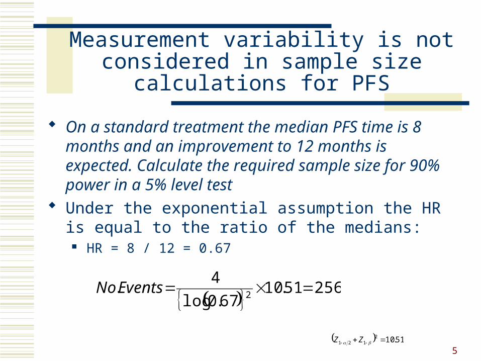
On a standard treatment the median PFS time is 8 months and an improvement to 12 months is expected. Calculate the required sample size for 90% power in a 5% level test

Under the exponential assumption the HR is equal to the ratio of the medians:

HR = 8 / 12 = 0.67

25651.10

67.0log

4. 2 EventsNo

51.102121 ZZ

5

Question addressed

In a comparative trial with a PFS endpoint, does measurement variability in the RECIST assessment impact the treatment effect Hazard Ratio (HR)?

RECIST: Response Evaluation Criteria in Solid Tumours

6

Assessment of target lesions (as per RECIST criteria) is subject to

measurement variability

10 cm

8 cm7 cm 7.5 cm 8.4 cm

30% in sum of the

LD = PR20% in sum of LD

(from nadir) = PD

Baseline

8 wk 16 wk 24 wk 32 wk

Tumour assessment is subject to measurement variability

7

What degree of measurement variability might we expect in

RECIST assessment?

In Non Small Cell Lung Cancer within subject variability was SD = 0.077cm (log scale) for repeat measurements (Zhao 2009)

E.g. For a mean tumour burden of 2 cm, a second scan will yield a measurement of approx 1.7 to 2.3 cm, 95% of the time

SD=0.077 cm may be an underestimate as this study only looked at single lesions

We therefore investigated multiples of this SD (2x and 3x) A review of SDs across tumour types was performed and is

reported in the paper Studies looking at the sum of target lesions were not found

8

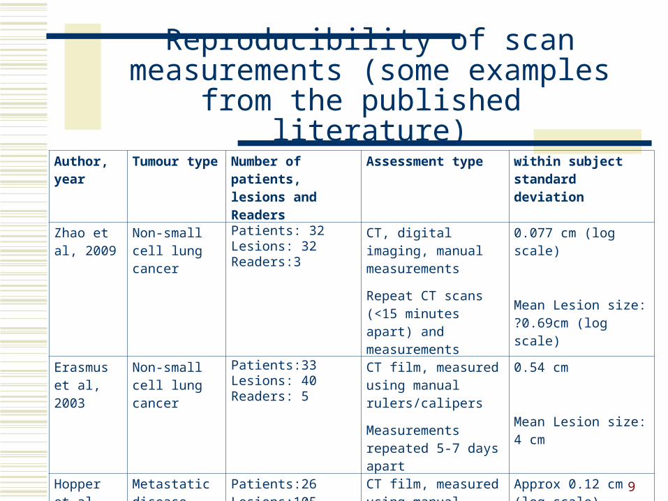
Reproducibility of scan measurements (some examples from the published literature)

Author, year

Tumour type

Number of patients, lesions and Readers

Assessment type within subject standard deviation

Zhao et al, 2009

Non-small cell lung cancer

Patients: 32 Lesions: 32 Readers:3

CT, digital imaging, manual measurements

Repeat CT scans (<15 minutes apart) and measurements

0.077 cm (log scale)

Mean Lesion size: ?0.69cm (log scale)

Erasmus et al, 2003

Non-small cell lung cancer

Patients:33 Lesions: 40 Readers: 5

CT film, measured using manual rulers/calipers

Measurements repeated 5-7 days apart

0.54 cm

Mean Lesion size: 4 cm

Hopper et al, 1996

Metastatic disease, thoracic and abdominal

Patients:26 Lesions:105 Readers: 3

CT film, measured using manual rulers/calipers

Repeat measurements

Approx 0.12 cm (log scale)

Mean Lesion size: 1.95cm (log scale)

9

Methods – A Simulation Study

Question addressed: In a comparative trial with a PFS endpoint, does measurement variability in the RECIST assessment impact the treatment effect HR?

10

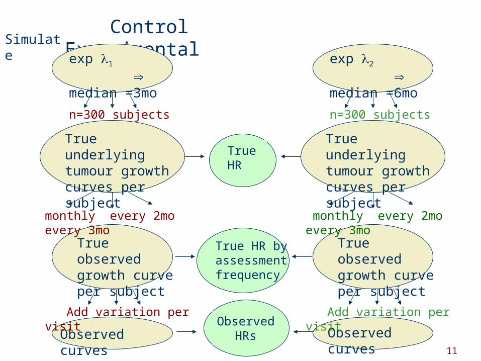
Control Experimental

Simulate

Observed curves Observed curves

exp 1 median =3mo

n=300 subjects

exp 2 median =6mo

n=300 subjects

True observed growth curve per subject

True observed growth curve per subject

Add variation per visit Add variation per visit

True underlying tumour growth curves per subject

True underlying tumour growth curves per subject

monthly every 2mo every 3mo

monthly every 2mo every 3mo

True HR

True HR by assessment frequency

Observed HRs

11

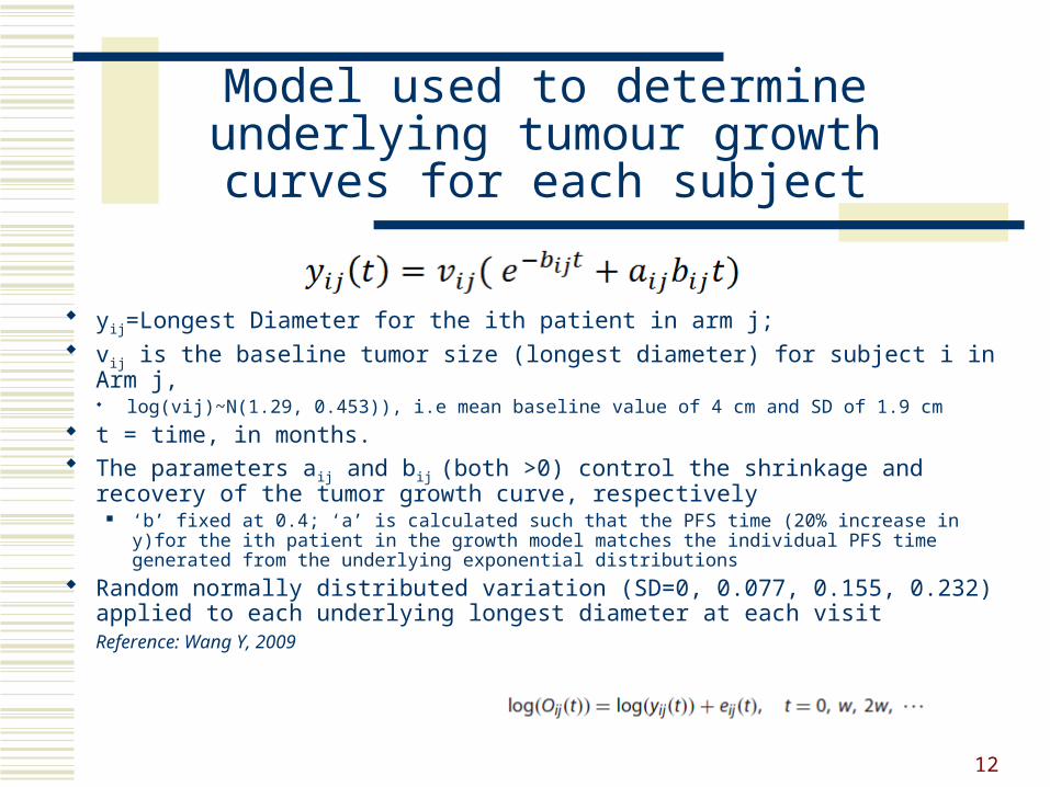
Model used to determine underlying tumour growth curves

for each subject

yij=Longest Diameter for the ith patient in arm j; vij is the baseline tumor size (longest diameter) for subject i in Arm j,

log(vij)~N(1.29, 0.453)), i.e mean baseline value of 4 cm and SD of 1.9 cm t = time, in months. The parameters aij and bij (both >0) control the shrinkage and recovery of

the tumor growth curve, respectively ‘b’ fixed at 0.4; ‘a’ is calculated such that the PFS time (20% increase in y)for the ith

patient in the growth model matches the individual PFS time generated from the underlying exponential distributions

Random normally distributed variation (SD=0, 0.077, 0.155, 0.232) applied to each underlying longest diameter at each visit Reference: Wang Y, 2009

12

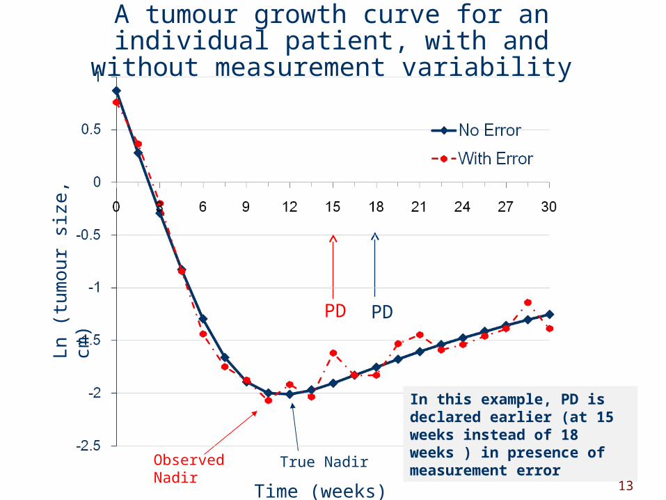
A tumour growth curve for an individual patient, with and without measurement

variability

Observed Nadir True Nadir

PD PD

In this example, PD is declared earlier (at 15 weeks instead of 18 weeks ) in presence of measurement error

Ln (

tum

ou

r si

ze,

cm)

Time (weeks) 13

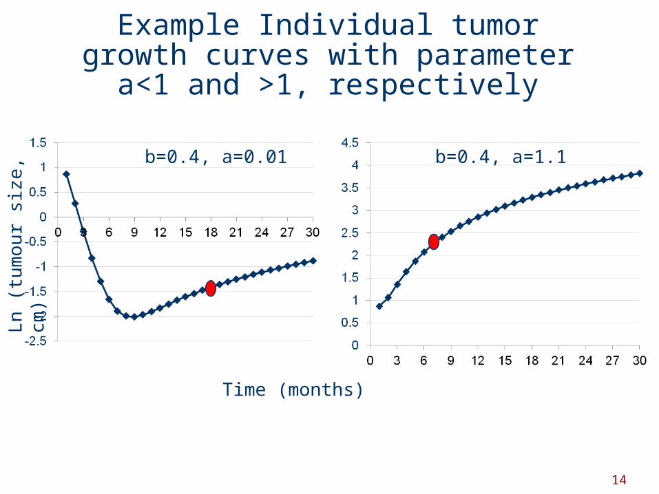
b=0.4, a=0.01 b=0.4, a=1.1

Ln (

tum

ou

r si

ze,

cm)

Time (months)

Example Individual tumor growth curves with parameter a<1 and

>1, respectively

14

Results

15

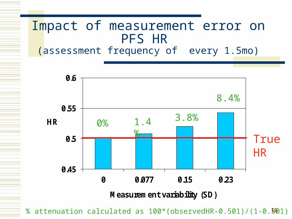
Impact of measurement error on PFS HR

(assessment frequency of every 1.5mo)

0.45

0.5

0.55

0.6

0 0.077 0.15 0.23

HR

Measurement variability (SD)

True HR

1.4%

3.8%

8.4%

0%

% attenuation calculated as 100*(observedHR-0.501)/(1-0.501) 16

Attenuation of the HR leads to a loss of statistical power (i.e. an

increase in type II error)

For example, for a trial that is to be sized with 90% power to detect a true HR=0.5, would have only 82% power to detect an attenuated HR=0.55 i.e. a loss of about 8% in power

Increasing levels of attenuation, lead to increased loss in statistical power

17

18

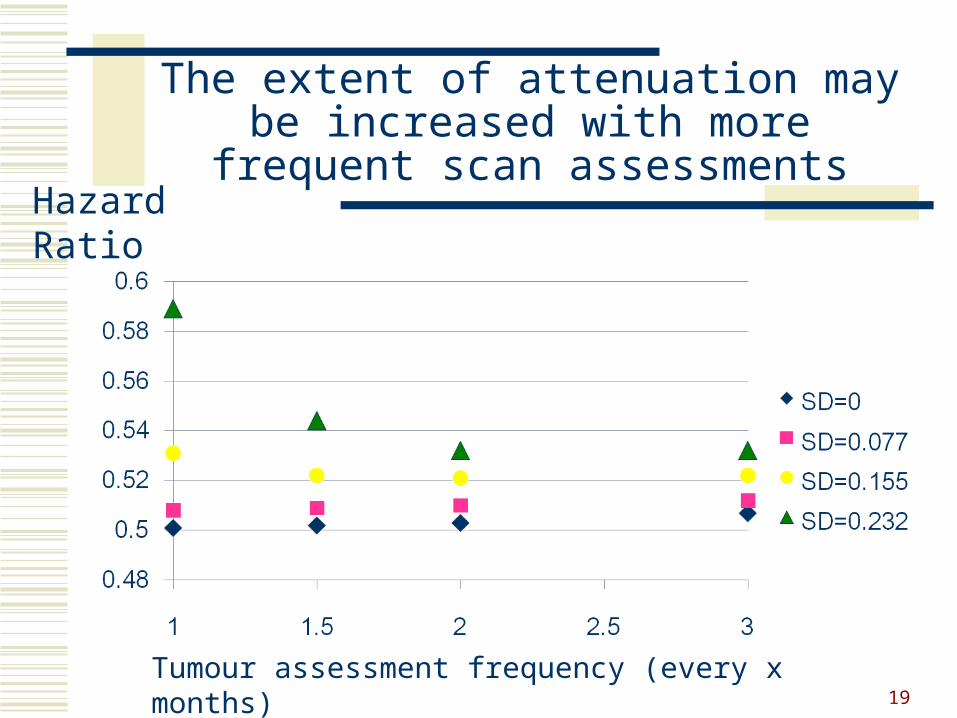
The extent of attenuation may be increased with more frequent scan

assessments

Tumour assessment frequency (every x months)

Hazard Ratio

19

Conclusions

Scan measurement variability can cause attenuation of the treatment effect (i.e. the HR is closer to one)

Scan measurement variability should be minimised in order to:

reveal a treatment effect that is closest to the truth Increase our the ability to identify valuable new therapies

In disease settings where the measurement variability is shown to be large, consideration may be given to

inflating the sample size of the study to maintain power Consider change of primary endpoint to overall survival?

The extent of attenuation may be increased with more frequent scan assessments

20

Some practical things we can do in our trials

Rigorous training of radiologists to ensure high-quality scans

The same radiologist should be used to read all scans from all patients at a particular site (or as a minimum all scans for an individual patient)

Are there ways to minimise the dilution requiring additional reads?

Note: RECIST guidance may ultimately help reduce measurement variability as fewer lesions (up to 5, reduced from 10) will be selected

21

Limitations

The model only considers progression of target (measurable) lesions and not new lesions

For some tumour types, a proportion of patients typically progress due to the appearance of new lesions

The model used may oversimplify the complexity of tumor growth

Choice of values for parameters a and b – are these realistic? This could be tested on existing clinical data

Have we underestimated the level of variability? variability typically calculated for repeat measurements of

individual lesions rather than for the sum of the longest diameters.

22

References

Eisenhauer EA, et al. New response evaluation criteria in solid tumours: Revised RECIST guideline (version 1.1). European J. Cancer 45:228-247, 2009

Erasmus JJ, Gladish GW, Broemeling L, et al. Interobserver and intraobserver variability in measurement of non-small-cell carcinoma lung lesions: Implications for assessment if tumour response. J Clin Oncol 21:2574-2582, 2003

Hopper K, Kasales C, Van Slyke M. Analysis of interobserver and intraobserver variability in CT tumor measurements. AJR 167: 851-854, 1996

Korn EL, Dodd LE, Freidlin B. Measurement error in the timing of events: effect on survival analyses in randomized clinical trials. Clinical trials 7: 626-633, 2010

Wang Y, Sung C, Dartois C, et al. Elucidation of relationship between tumor size and survival in non-small-cell lung cancer patients can aid early decision making in clinical drug development. Clin. Pharm. Therapeutics 86:167-174, 2009

Zhao B, James LP, Moskowitz CS et al. Evaluating variability in tumor measurements from same-day repeat CT scans of patients with non-small cell lung cancer. Radiology. 252:263-272, 2009

23

24

Q?

25

Back-up

26

Definitions: Hazard Ratio

HR is the ratio of the hazard (progression) rates of the two groups HR=1 means no difference between

treatment in terms of progression rates HR=0.8 rate of progression decreased by

20%, or (take reciprocal) delays rate of progression by 25% (1/0.8=1.25)

HR=2 means risk on active group is twice that on control

27

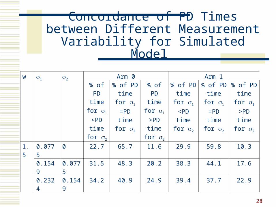
Concordance of PD Times between Different Measurement Variability

for Simulated Model

w 1 2 Arm 0 Arm 1% of PD time for 1 <PD

time for 2

% of PD time for 1 =PD

time for 2

% of PD time for 1 >PD

time for 2

% of PD time for 1 <PD

time for 2

% of PD time for 1 =PD

time for 2

% of PD time for 1 >PD

time for 2

1.5 0.0775 0 22.7 65.7 11.6 29.9 59.8 10.3

0.1549 0.0775 31.5 48.3 20.2 38.3 44.1 17.6

0.2324 0.1549 34.2 40.9 24.9 39.4 37.7 22.9

28

0

0.1

0.2

0.3

0.4

0.5

0.6

0.7

0.8

0.9

1

0 10 20 30 40 50T im e

Su

rviv

al

a rm 1

arm 2

0

0.1

0.2

0.3

0.4

0.5

0.6

0.7

0.8

0.9

1

0 10 20 30 40 50T im e

Su

rviv

al

a rm 1

arm 2

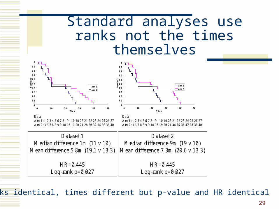
D ata Arm 1: 1 2 3 4 5 6 7 8 9 10 10 20 21 22 23 24 25 26 27Arm 2: 3 6 7 8 8 9 9 10 10 11 20 24 28 30 32 34 36 38 40

D ata Arm 1: 1 2 3 4 5 6 7 8 9 10 10 20 21 22 23 24 25 26 27Arm 2: 3 6 7 8 8 9 9 10 10 19 20 24 34 35 36 37 38 39 40

D ataset 1M edian difference 1m (11 v 10)

M ean difference 5 .8m (19.1 v 13.3)

H R =0.445Log-rank p=0.027

D ataset 2M edian difference 9m (19 v 10)

M ean difference 7 .3m (20.6 v 13.3)

H R =0.445Log-rank p=0.027

Standard analyses use ranks not the times themselves

Ranks identical, times different but p-value and HR identical

29

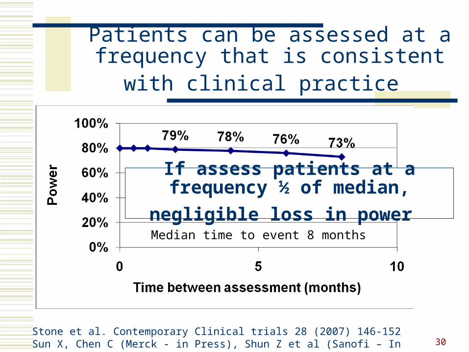
If assess patients at a frequency ½ of median,

negligible loss in power

Patients can be assessed at a frequency that is consistent with clinical practice

Median time to event 8 months

Stone et al. Contemporary Clinical trials 28 (2007) 146-152Sun X, Chen C (Merck - in Press), Shun Z et al (Sanofi – In Press) 30