attenuation, delay and noise properties of light slowed by

Attenuation, Delay and Noise properties of light

slowed by Electromagnetically Induced

Transparency.

Kerry B. Burke

A thesis submitted for the degree of

Bachelor of Philosophy with Honours in Physics of

The Australian National University

October, 2006

Declaration

This thesis is an account of research undertaken between February 2004 and October 2006

at The Department of Physics, Faculty of Science, The Australian National University,

Canberra, Australia.

Except where acknowledged in the customary manner, the material presented in this

thesis is, to the best of my knowledge, original and has not been submitted in whole or

part for a degree in any university.

Kerry B. Burke

October, 2006

iii

Acknowledgements

I would like to thank Ben Buchler and Magnus Hsu for putting up with my questions and

for all their help on the experiment and on the data processing. I’d like to thank Gabriel

Hetet and Oliver Glockl for their help with solving a few of the problems which cropped

up. I’d like to thank Nicolai Grosse for letting me use his equipment and Ping Koy Lam

for being my supervisor.

v

Abstract

Electromagnetically Induced Transparency is an effect that allows light to propagate

through an otherwise opaque material. Due to the dispersion properties of the EIT sys-

tem, it also slows the information carried on the sideband frequencies of a light beam.

The effect can also be used to store information in an atomic medium. It was thereforw

proposed that EIT systems can be applied in optical cicuits, specifically with regard to

quantum information processing where it is necessary to delay, or store quantum states of

light. Hence it is necessary to understand how EIT systems influence the quantum state

of a light beam and whether EIT systems can ever have the potential to delay and store

quantum information at the quantum noise limit.

This thesis examines the transfer of an optical signal at the sideband frequencies

through an EIT medium. A comprehensive characterisation of an EIT system in terms of

delay and signal transmission is performed. This measurement technique provides data

on EIT performance over a range of signal frequencies and a range of experimental pa-

rameters. Experiments were conducted with both pure Rubidium vapour and Rubidium

vapour mixed with a noble gas.

Studies have been made into a new system of measurement that will allow delay,

attenuation and added noise spectra to be assessed via a single-shot measurement.

vii

Contents

Declaration iii

Acknowledgements v

Abstract vii

1 Introduction 3

1.1 History . . . . . . . . . . . . . . . . . . . . . . . . . . . . . . . . . . . . . . 3

1.2 Motivation . . . . . . . . . . . . . . . . . . . . . . . . . . . . . . . . . . . . 4

1.3 Thesis Structure . . . . . . . . . . . . . . . . . . . . . . . . . . . . . . . . . 4

2 Theory 7

2.1 Electromagnetically Induced Transparency . . . . . . . . . . . . . . . . . . . 7

2.1.1 The Dark State . . . . . . . . . . . . . . . . . . . . . . . . . . . . . . 8

2.1.2 Equations of Motion . . . . . . . . . . . . . . . . . . . . . . . . . . . 9

2.2 Susceptibility and the Group Velocity . . . . . . . . . . . . . . . . . . . . . 10

2.3 Homodyne detectors . . . . . . . . . . . . . . . . . . . . . . . . . . . . . . . 13

2.4 Conditional Variance . . . . . . . . . . . . . . . . . . . . . . . . . . . . . . . 14

2.4.1 Ideal Conditional Variance . . . . . . . . . . . . . . . . . . . . . . . 15

2.4.2 Practical Conditional Variance Measurement . . . . . . . . . . . . . 16

3 Experiment 19

3.1 Laser Source . . . . . . . . . . . . . . . . . . . . . . . . . . . . . . . . . . . 19

3.1.1 The Laser . . . . . . . . . . . . . . . . . . . . . . . . . . . . . . . . . 19

3.1.2 Multimode Behaviour . . . . . . . . . . . . . . . . . . . . . . . . . . 20

3.1.3 Feedback . . . . . . . . . . . . . . . . . . . . . . . . . . . . . . . . . 20

3.1.4 Mode Quality . . . . . . . . . . . . . . . . . . . . . . . . . . . . . . . 20

3.2 Rubidium Structure . . . . . . . . . . . . . . . . . . . . . . . . . . . . . . . 20

3.3 Laser Frequency Control . . . . . . . . . . . . . . . . . . . . . . . . . . . . . 22

3.3.1 Doppler Broadening . . . . . . . . . . . . . . . . . . . . . . . . . . . 22

3.3.2 Saturated Absorption Spectroscopy . . . . . . . . . . . . . . . . . . . 23

3.4 Locking Loops . . . . . . . . . . . . . . . . . . . . . . . . . . . . . . . . . . 24

3.5 Beam preparation . . . . . . . . . . . . . . . . . . . . . . . . . . . . . . . . 27

3.6 Rubidium Cell . . . . . . . . . . . . . . . . . . . . . . . . . . . . . . . . . . 27

3.7 Homodyne Detectors . . . . . . . . . . . . . . . . . . . . . . . . . . . . . . . 28

3.8 Data Acquisition . . . . . . . . . . . . . . . . . . . . . . . . . . . . . . . . . 29

3.8.1 Network Analyser . . . . . . . . . . . . . . . . . . . . . . . . . . . . 29

3.8.2 PXI . . . . . . . . . . . . . . . . . . . . . . . . . . . . . . . . . . . . 29

3.9 Data Processing . . . . . . . . . . . . . . . . . . . . . . . . . . . . . . . . . 29

3.9.1 Delay measurement . . . . . . . . . . . . . . . . . . . . . . . . . . . 29

3.9.2 Normalisation to Quantum Noise . . . . . . . . . . . . . . . . . . . . 30

3.9.3 Conditional Variance and Attenuation . . . . . . . . . . . . . . . . . 30

ix

x Contents

4 Results 31

4.1 Laser Noise . . . . . . . . . . . . . . . . . . . . . . . . . . . . . . . . . . . . 31

4.2 Delay Measurements . . . . . . . . . . . . . . . . . . . . . . . . . . . . . . . 32

4.2.1 Unbuffered Rubidium Cell . . . . . . . . . . . . . . . . . . . . . . . . 32

4.2.2 Buffered Rubidium Cell . . . . . . . . . . . . . . . . . . . . . . . . . 34

4.2.3 Spatial Effects . . . . . . . . . . . . . . . . . . . . . . . . . . . . . . 36

4.3 PXI Measurements and Post Processing . . . . . . . . . . . . . . . . . . . . 36

4.3.1 Noise Characteristics of the Measurement System . . . . . . . . . . . 36

4.3.2 Post Processed Delay Measurements . . . . . . . . . . . . . . . . . . 37

4.3.3 Post Processed Attenuation Measurements . . . . . . . . . . . . . . 37

4.3.4 Conditional Variance . . . . . . . . . . . . . . . . . . . . . . . . . . . 38

5 Conclusion and Future Directions 41

5.1 Conclusions . . . . . . . . . . . . . . . . . . . . . . . . . . . . . . . . . . . . 41

5.2 Future Directions . . . . . . . . . . . . . . . . . . . . . . . . . . . . . . . . . 41

Bibliography 43

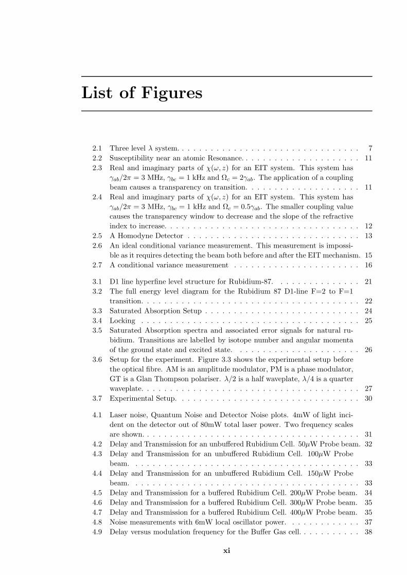
List of Figures

2.1 Three level λ system. . . . . . . . . . . . . . . . . . . . . . . . . . . . . . . . 7

2.2 Susceptibility near an atomic Resonance. . . . . . . . . . . . . . . . . . . . . 11

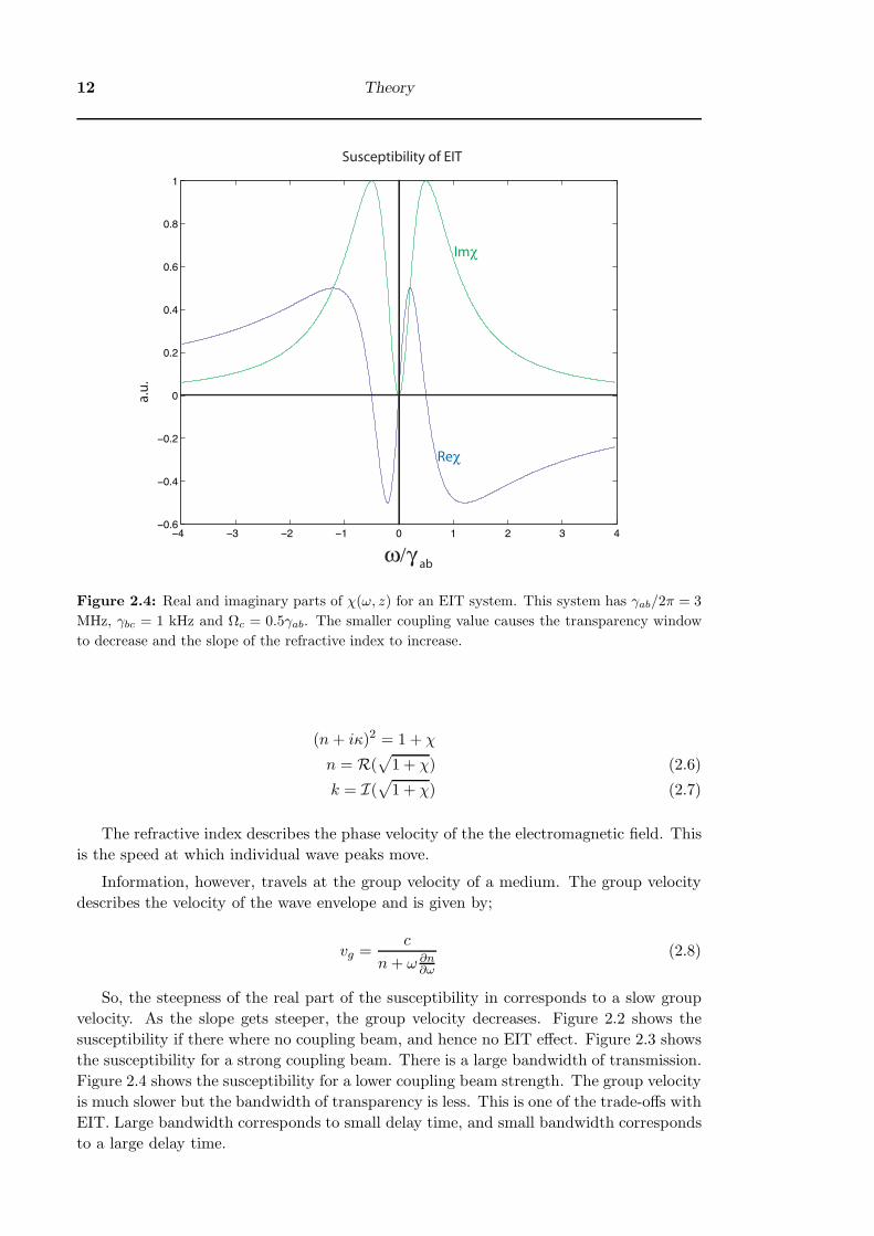
2.3 Real and imaginary parts of χ(ω, z) for an EIT system. This system has

γab/2π = 3 MHz, γbc = 1 kHz and Ωc = 2γab. The application of a coupling

beam causes a transparency on transition. . . . . . . . . . . . . . . . . . . . 11

2.4 Real and imaginary parts of χ(ω, z) for an EIT system. This system has

γab/2π = 3 MHz, γbc = 1 kHz and Ωc = 0.5γab. The smaller coupling value

causes the transparency window to decrease and the slope of the refractive

index to increase. . . . . . . . . . . . . . . . . . . . . . . . . . . . . . . . . . 12

2.5 A Homodyne Detector . . . . . . . . . . . . . . . . . . . . . . . . . . . . . . 13

2.6 An ideal conditional variance measurement. This measurement is impossi-

ble as it requires detecting the beam both before and after the EIT mechanism. 15

2.7 A conditional variance measurement . . . . . . . . . . . . . . . . . . . . . . 16

3.1 D1 line hyperfine level structure for Rubidium-87. . . . . . . . . . . . . . . 21

3.2 The full energy level diagram for the Rubidium 87 D1-line F=2 to F=1

transition. . . . . . . . . . . . . . . . . . . . . . . . . . . . . . . . . . . . . . 22

3.3 Saturated Absorption Setup . . . . . . . . . . . . . . . . . . . . . . . . . . . 24

3.4 Locking . . . . . . . . . . . . . . . . . . . . . . . . . . . . . . . . . . . . . . 25

3.5 Saturated Absorption spectra and associated error signals for natural ru-

bidium. Transitions are labelled by isotope number and angular momenta

of the ground state and excited state. . . . . . . . . . . . . . . . . . . . . . 26

3.6 Setup for the experiment. Figure 3.3 shows the experimental setup before

the optical fibre. AM is an amplitude modulator, PM is a phase modulator,

GT is a Glan Thompson polariser. λ/2 is a half waveplate, λ/4 is a quarter

waveplate. . . . . . . . . . . . . . . . . . . . . . . . . . . . . . . . . . . . . . 27

3.7 Experimental Setup. . . . . . . . . . . . . . . . . . . . . . . . . . . . . . . . 30

4.1 Laser noise, Quantum Noise and Detector Noise plots. 4mW of light inci-

dent on the detector out of 80mW total laser power. Two frequency scales

are shown. . . . . . . . . . . . . . . . . . . . . . . . . . . . . . . . . . . . . . 31

4.2 Delay and Transmission for an unbuffered Rubidium Cell. 50µW Probe beam. 32

4.3 Delay and Transmission for an unbuffered Rubidium Cell. 100µW Probe

beam. . . . . . . . . . . . . . . . . . . . . . . . . . . . . . . . . . . . . . . . 33

4.4 Delay and Transmission for an unbuffered Rubidium Cell. 150µW Probe

beam. . . . . . . . . . . . . . . . . . . . . . . . . . . . . . . . . . . . . . . . 33

4.5 Delay and Transmission for a buffered Rubidium Cell. 200µW Probe beam. 34



4.8 Noise measurements with 6mW local oscillator power. . . . . . . . . . . . . 37

4.9 Delay versus modulation frequency for the Buffer Gas cell. . . . . . . . . . . 38

xi

LIST OF FIGURES 1

4.10 Gain calculated using post-processed PXI data. . . . . . . . . . . . . . . . . 39

4.11 Conditional Variance, normalised to Quantum Noise and via Equation 2.16 40

4.12 Normalisation test of Conditional Variance algorithm. . . . . . . . . . . . . 40

2 LIST OF FIGURES

Chapter 1

Introduction

Electromagnetically Induced Transparency (EIT) is a physical effect where a laser beam is

used to change an opaque material so that light can pass through it. This effect also causes

a reduction in the speed of information carried by the light. The ability to delay light is

of crucial importance for synchronising optical circuits, particularly in the emerging field

of quantum information science. Aside from the practical applications, understanding the

details of this effect will give greater understanding of atom-light interactions in general.

1.1 History

The groundwork for EIT is a process called Coherent Population Trapping (CPT), first

demonstrated in 1976 by Alzetta et.al. [1]. To briefly explain this effect I will adapt an

explanation given by Harris [2]. Classically, the interaction of light and matter can be

understood as the light causing the electrons to vibrate at a certain frequency. If the

electrons are vibrating at a very specific frequency then they will undergo a transition

to another energy state. If two vibrations were out of phase, then their effects would

destructively interfere. This would mean that the electrons could not vibrate at that

specific frequency and so could not undergo a transition to an excited state. This coherence

effect causes the population of electrons to be trapped in the lower energy states.

EIT was first demonstrated in 1991 [3] where it was shown that Strontium vapour

could be made transparent. CPT is the mechanism that allows EIT to work. Classically,

light is absorbed when it drives an electron into a higher energy state. If this energy state

is forbidden by CPT, then light cannot be absorbed and the material becomes transparent.

Eight years later, slowing of light pulses was demonstrated using EIT in a Bose-Einstein

Condensate of Sodium atoms [4]. In a Bose-Einstein Condensate, atoms are so cold that

they are effectively stationary and occupy the same quantum state. In this experiment

light pulses were slowed down to 17ms−1, showing that EIT also causes a reduction in the

group velocity of light.

Since these pulses of light were travelling so slowly, they were spatially compressed as

well. They could be compressed enough so that the entire pulse fitted inside the atomic

medium. Philips et. al. [5] showed that if the coupling laser beam was turned off while

the pulse was inside the medium, then the pulse was stored and could be later retrieved

by turning on the coupling laser beam. Philips et. al. [5] and later Bajcsy et. al. [6]

showed that pulses of light could be stored in atomic vapour cells.

Liu et.al. [7] showed that storage of pulses was possible in a cold atomic cloud. Slow

light and pulse storage via EIT have also been observed in cryogenic solids [8], with a

record delay time of greater than one second being set by Longdell et. al. [9]. Other

impressive results include storage of single photons by Chaneliere et. al. [10].

3

4 Introduction

In continuous wave experiments, group velocities of 90ms−1 where achieved for an

optical beam in a hot Rubidium gas [11]. Heated Rubidium vapour is the material used in

the experiments of this thesis, the main advantage of the material being that experiments

can be conducted at room temperature.

Theoretical calculations [12, 13, 14, 15] have claimed that the effect of EIT can delay

a squeezed or entangled state. As there is very little absorption of the light, only a small

amount of vacuum noise should degrade the squeezed or entangled state, enabling EIT

to be used as a quantum limited delay device. Akamatsu et. al. [16] have shown that a

squeezed state can survive transmission through an EIT medium, although this was under

the conditions of very small delay times.

However, Hsu et. al. [17] have shown that a continuous wave signal delayed using EIT

in a hot Rubidium gas experiences a lot more added noise than theoretical calculations

would suggest. The source of this extra noise is not understood and it can only be identified

by varying parameters of the experiment and determining which parameters make a change

to the amount of added noise. Atomic decoherences in the form of Radiation Trapping [18]

or atomic collisions have been suggested as mechanisms by which this extra noise could

be added to the system.

Experimental results of light storage via EIT have been called into question by Alek-

sandrov and Zapasskii [19], [20] claiming that the delay phenomena observed have for

the most part been over interpreted and that the pulse delays observed can be explained

in terms of much simpler physics. The results have also been called into question after

Akulshin et. al. [21] demonstrated qualitatively similar results to those of Phillips et. al.

[5] under experimental conditions where EIT was not possible. The main criticism is that

Saturable Absorption causes pulse-reshaping. If the group velocity is defined as the speed

of the peak of a pulse, and if the pulse is reshaped, then the speed of the peak of a pulse

is no longer an accurate measure of the group velocity.

Selden [22] listed criteria that would confirm that delays were due to EIT and not due

to Saturable Absorption effects. The most relevant of these is that a continuous wave

signal must be delayed by at least a quarter of a cycle for the delay to unambiguously be

ascribed to EIT.

1.2 Motivation

What is not well known is the source of the extra noise found by Hsu et. al. [17]. One

of the effects that EIT relies upon is Coherent Population Trapping. If the atoms were to

lose their coherence with each other then noise could be added to the light transmitted

through an EIT system. Given that the material we are working with is a hot atomic

vapour, atom-atom collisions could easily introduce decoherences.

It is also desirable to develop techniques to quickly measure the noise added to the

system. I have worked on post-processing digitally acquired data to measure conditional

variance, which is a measure of noise. These measurements could theoretically be made

single-shot.

1.3 Thesis Structure

This thesis is broken into Theory, Experiment and Results Section. The Theory section

covers the background theory of EIT and Conditional Variance measurements. Conditional

§1.3 Thesis Structure 5

variance is a measure of the sameness of two signals and is used to calculate the noise added

to a signal by EIT. The experimental section covers all aspects of the experiment, from

the laser itself, to the structure of the atoms, to the detection systems used. Results shows

the results I was able to obtain, and details some of the difficulties encountered.

6 Introduction

Chapter 2

Theory

The aim of this experiment is to measure properties of the EIT system, specifically delay,

attenuation and added noise as a function of sideband frequency. It is necessary to un-

derstand what mechanism creates the transparency and delay. Also, to properly choose

what measurements to take and how to analyse the data it is necessary to consider some

quantum optics theory.

2.1 Electromagnetically Induced Transparency

In this treatment of EIT the coupling beam will be assumed to be classical, and much larger

than the probe field. The probe field and atoms will be treated quantum mechanically. It

is also assumed that there is no detuning from the atomic transitions.

The following equation for the system’s Hamiltonian comes from [23] Eq. (2.15).

the detuning terms in the original equation have been dropped. Many of the following

equations have been adapted from [23] chapter 2.

Hint = − hN

l

∫

gE(z.t)σab(z.t) + gE†(z, t)σba(z, t) + Ωcσac(z, t) + Ωcσca(z, t) dz (2.1)

The Hamiltonian has been written in terms of the atomic operators (σµν), the probe

field operator (E) and the Rabi frequency (Ωc), taken to be real, of the coupling beam.

|a

|b |c

Ω c

γbc

γab

γac

Figure 2.1: Three level λ system.

7

8 Theory

g = dba

√

ωab/2ǫ0V h is the atom-field coupling constant, where dba is the atomic dipole

moment of the transition and ωba is the frequency of the transition. N is the number of

atoms, l is length of the cell.

The atomic operators (σµν) refer to a class of atoms with zero velocity

σµν(z, t) =1

nAδz

∑

zj∈[z,z+δz]

σjµν(z, t)ei

ωµν

c(zj−ct)

Where n is the number of atoms, A is the area of a small transverse slice of the cell

and σjµν is the jth atom in the small volume Aδz.

2.1.1 The Dark State

The eigenstate of this Hamiltonian is special in that it has no population in the excited

state |a〉. This means the state cannot spontaneously emit light, hence it is called a dark

state.

To calculate the eigenstate of the Hamiltonian, the probe beam will be treated classi-

cally, and the spatial dependance will be removed. This simplified Hamiltonian is then;

Hint = −hNΩp(t)σab(t) + Ω∗p(t)σba(t) + Ωcσac(t) + Ωcσca(t)

Where Ωp = g〈E〉. The eigenstate of this Hamiltonian is found by;

Hint (a(t)|a〉 + b(t)|b〉 + c(t)|c〉) = λ (a(t)|a〉 + b(t)|b〉 + c(t)|c〉)

−hN(

gΩp(t)b(t)|a〉 + Ω∗p(t)a(t)|b〉 + Ωcc(t)|a〉 + Ωca(t)|c〉

)

= λ (a(t)|a〉 + b(t)|b〉 + c(t)|c〉)

Equating coefficients of the basis states gives;

Ωca(t) = λc(t)

gΩ∗p(t)a(t) = λb(t)

gE(t)b(t) + Ωcc(t) = λa(t)

The only nontrivial solution to this is;

λ = 0

a(t) = 0

b(t) = Ωc

c(t) = −Ωp(t)

As explained before, this eigenstate has no population in the exited state |a〉. Therefore

atoms cannot spontaneously emit light and there is very little absorption. The lack of

spontaneous emission earns this eigenstate the name ’Dark State’. The dark state is a

superposition of the two ground states.

§2.1 Electromagnetically Induced Transparency 9

|D〉 =Ωc|b〉 − Ωp(t)|c〉

√

|Ωc|2 + |Ωp(t)|2

2.1.2 Equations of Motion

Assuming there is no decoherence, i.e. an ideal three level system. The equations of

motion of the atomic operators comes from the Hamiltonian (Eq. 2.1) via the Schroedinger

equation. From here on the space and time dependance of the atomic and probe field

operators will not be explicitly shown.

ih∂σµν

∂t= [σµν , Hint]

˙σaa = ig(E σab − E†σba) + iΩc(σac − σca)

˙σbb = ig(−E σab + E†σba)

˙σcc = iΩc(−σac + σca)

˙σba = ig(E σbb − E†σaa) + iΩcσbc

˙σbc = −igE σac + iΩcσba

˙σac = −igE†σbc + iΩc(σaa − σcc)

Spontaneous emission, and decoherence are two loss effects which need to be accounted

for. These efffects are represented by the γ terms. To preserve the commutation relations

it is necessary to add the Langevin noise operators, represented by the F terms. These

terms can be phenomenologically added to the equations of motion, although they can

also be added rigourously.

˙σaa = −γaaσaa + ig(E σab − E†σba) + iΩc(σac − σca) + Faa

˙σbb = γbbσaa + ig(−E σab + E†σba) + Fbb

˙σcc = γccσaa + iΩc(−σac + σca) + Fcc

˙σba = −γbaσba + ig(E σbb − E†σaa) + iΩcσbc + Fba

˙σbc = −γbcσbc − igE σac + iΩcσba + Fbc

˙σac = −γabσac − igE†σbc + iΩc(σaa − σcc) + Fac

The Maxwell equation to describe light in this medium is;

(

∂

∂t+ c

∂

∂z

)

E = ig∗Nσba

It has been assumed that the coupling beam is much stronger than the probe beam. It

is also assumed that in the initial state the entire population is in |b〉 so σbb = 1. Then σaa

and σac are zero to first order. Also the probe beam has a signal on it and so is a function

of time, whereas the coupling beam is roughly constant. Hence the following equations

can be formed.

10 Theory

˙σba = −γbaσba + igE(t) + iΩcσbc + Fba

˙σbc = −γbcσbc + iΩcσba + Fbc

These equations can be solved by transforming to Fourier Space via

O(z, ω) =1√2π

∫ ∞

−∞O(z, t)eiωt dt

Giving;

−iωσba = −γbaσba + igE(ω) + iΩcσbc + Fba

−iωσbc = −γbcσbc + iΩcσba + Fbc(

−iω + c∂

∂z

)

E = ig∗Nσba (2.2)

At this point we are only interested in deriving the susceptibility of the EIT medium.

Only the classical terms are needed for this. σµν will be replaced with 〈σµν〉, the probe

field gE will be instead written as a Rabi frequency Ωc, and the Langevin operators will be

ignored. A full quantum treatment of these equations is given in ref. [23], the conclusion

reached there is that the Langevin operators only add the amount of vacuum noise expected

from the absorption of the medium. So, disregarding the Langevin operators, the equations

2.2 can be written as;

|g|2Nc (γbc − iω)

(γba − iω)(γbc − iω) + Ω2c

− iω + c∂

∂z

Ωp = 0

let

Λ(ω, z) =|g|2N

c (γbc − iω)

(γba − iω)(γbc − iω) + Ω2c

− iω (2.3)

then;

Ωp

(

l

2, ω

)

= e−

∫ l2

−

l2

Λ(ω,z) dzΩp

(

− l

2, w

)

(2.4)

Equation 2.4 can be interpreted as the probe beam being attenuated and phase shifted

by Λ(ω, z).

The probe susceptibility is defined as;

ik

2χ(ω, z) = −

(

Λ(ω, z) +iω

c

)

(2.5)

2.2 Susceptibility and the Group Velocity

The susceptibility of a medium determines both the refractive index, n, and the absorption

coefficient, κ.

§2.2 Susceptibility and the Group Velocity 11

−4 −3 −2 −1 0 1 2 3 4−0.6

−0.4

−0.2

0

0.2

0.4

0.6

0.8

1

ω/γab

Reχ

Imχa.

u.

Susceptibility of EIT

Figure 2.2: Real and imaginary parts of χ(ω, z) for a typical two level system. This is what the

susceptibility looks like when the coupling beam is turned off and there is no EIT.

−4 −3 −2 −1 0 1 2 3 4−0.6

−0.4

−0.2

0

0.2

0.4

0.6

0.8

1

ω/γab

Reχ

Imχ

a.u

.

Susceptibility of EIT

Figure 2.3: Real and imaginary parts of χ(ω, z) for an EIT system. This system has γab/2π = 3

MHz, γbc = 1 kHz and Ωc = 2γab. The application of a coupling beam causes a transparency on

transition.

12 Theory

−4 −3 −2 −1 0 1 2 3 4−0.6

−0.4

−0.2

0

0.2

0.4

0.6

0.8

1

ω/γab

Reχ

Imχ

a.u

.Susceptibility of EIT

Figure 2.4: Real and imaginary parts of χ(ω, z) for an EIT system. This system has γab/2π = 3

MHz, γbc = 1 kHz and Ωc = 0.5γab. The smaller coupling value causes the transparency window

to decrease and the slope of the refractive index to increase.

(n + iκ)2 = 1 + χ

n = R(√

1 + χ) (2.6)

k = I(√

1 + χ) (2.7)

The refractive index describes the phase velocity of the the electromagnetic field. This

is the speed at which individual wave peaks move.

Information, however, travels at the group velocity of a medium. The group velocity

describes the velocity of the wave envelope and is given by;

vg =c

n + ω ∂n∂ω

(2.8)

So, the steepness of the real part of the susceptibility in corresponds to a slow group

velocity. As the slope gets steeper, the group velocity decreases. Figure 2.2 shows the

susceptibility if there where no coupling beam, and hence no EIT effect. Figure 2.3 shows

the susceptibility for a strong coupling beam. There is a large bandwidth of transmission.

Figure 2.4 shows the susceptibility for a lower coupling beam strength. The group velocity

is much slower but the bandwidth of transparency is less. This is one of the trade-offs with

EIT. Large bandwidth corresponds to small delay time, and small bandwidth corresponds

to a large delay time.

§2.3 Homodyne detectors 13

-

ab

cd

Piezoelectric Crystal

Figure 2.5: A Homodyne Detector

2.3 Homodyne detectors

The amplitude and phase of light are conjugate variables. It is only possible to measure

one or the other without incurring a noise penalty. Amplitude quadrature is defined by;

X0 = a + a†

Phase quadrature is defined by;

Xπ/2 = i(a − a†)

In this experiment I detect δX0 at the sideband frequencies.

A homodyne detector is used to make measurements of either the amplitude or phase

quadrature of light. Consider two input optical fields, a and b, incident on a 50-50 beam-

splitter. The two optical fields will interfere and two beams, c and d will result. The

detectors measure the fields c and d given by;

c =

√

1

2(a + b)

d =

√

1

2(a − b)

Each detector has a photocurrent proportional to c†c and d†d respectively.

c†c =1

2(a†a + b†b + a†b + b†a)

d†d =1

2(a†a + b†b − a†b − b†a)

The difference of the detector photocurrents is then;

c†c − d†d = a†b + b†a

The field can be written in terms of a mean and fluctuations about the mean. a = A+δa

where A = 〈a〉. Also, as the two beams come from the same source, they must have the

same frequency. We can write a phase difference θ between the fields.

a = (A + δa)eiθ

b = B + δb

c†c − d†d =(

(A + δa†)eiθ(B + δb) + (B + δb†)(A + δa)eiθ)

14 Theory

Making the approximation that the fluctuations are small compared to the mean field,

the δb and δa cross terms are discarded.

c†c − d†d = 2AB cos θ + A(δbe−iθ + δb†eiθ) + B(δaeiθ + δa†e−iθ)

Now in the case of the homodyne detector, one input is the signal. The other input is

the local oscillator and is much larger than the signal. So we assume A ≫ B.

c†c − d†d = 2AB cos θ + AδXθb

By varying θ either the amplitude or phase quadrature can be detected. Experimentally

θ can be adjusted by applying a voltage to a piezoelectric crystal mounted on a mirror

where the mirror reflects one of the input beams. See figure 2.5. Changing the piezoelectric

crystal changes the path length difference between the two beams.

2.4 Conditional Variance

A signal on a laser field will be written as X in the time domain and as X in the frequency

domain. δX refers to the AC component of the field.

The variance of a signal describes how much power is in the fluctuations about the

mean field and is given by;

V =⟨

|δX |2⟩

The correlation between two signals X1 and X2 is given by;

C1,2 =

⟨

δX1δX2

⟩

√V1V2

A correlation of 1 means that the two signals are the same.

The correlation, however, will show two signals as less than perfectly correlated if one

signal is attenuated with respect to another.

The conditional variance is a measure of signal similarity independent of attenuation.

It is defined by;

V1|2 = V1(1 − C21,2) (2.9)

If the two signals are the same it can be seen that the conditional variance is zero and

if the if the two signals are uncorrelated then the conditional variance is just the V1.

This is is equivalent to the following definition. We want find the difference between

to signals, and we want it to be independent of the scale of the two signals. So minimise

the difference between two signals after scaling one of them by a gain factor.

V1|2 = ming

⟨

|δX1 − gδX2|⟩

(2.10)

V1|2 = ming

〈δX21 〉 − 2g〈δX1δX2〉 + g2〈δX2

2 〉 (2.11)

V1|2 = ming

V1 − 2gC1,2

√

V1V2 + g2V2 (2.12)

§2.4 Conditional Variance 15

η(ω) +X n

v2X

L.O.

- outXsX

L.O.

-

Figure 2.6: An ideal conditional variance measurement. This measurement is impossible as it

requires detecting the beam both before and after the EIT mechanism.

The optimum g is given by setting the derivative to zero.

0 = −2C1,2

√

V1V2 + 2gV2

g = C1,2

√

V1

V2

Substituting this back into Equation 2.12.

V1|2 = V1 − 2C21,2V1 + C1,2V1 (2.13)

V1|2 = V1(1 − C21,2) (2.14)

Which is the same as Equation 2.9. By substituting in the definition of the correlation

the conditional variance is;

V1|2 = V1 −

∣

∣

∣

⟨

δX1δX2

⟩∣

∣

∣

2

V2

2.4.1 Ideal Conditional Variance

Figure 2.6 shows an experimental setup for an ideal conditional variance measurement. It

requires the impossible step of detecting both the incoming beam and the outgoing beam.

Xs is the signal encoded on the beam, Xv2 is a vacuum noise term due to attenuation by

EIT and Xn is any additional noise added by the EIT system not accounted for by the

Langevin noise operators. Xout is the signal after modification by the EIT medium.

The Conditional Variance between Xout and Xs is.

Vout|s = Vout −

∣

∣

∣〈δXsδXout〉∣

∣

∣

2

Vs

Vout|s = η(ω)Vs + (1 − η(ω)) + Vn −

∣

∣

∣

⟨

δXs

(

√

η(ω)δXs +√

1 − η(ω)δXv2 + δXn

)⟩∣

∣

∣

2

Vs

Vout|s = η(ω)Vs + 1 − η(ω) + Vn −

∣

∣

∣

√

η(ω)Vs

∣

∣

∣

2

Vs

16 Theory

-

η(ω) +X ns

v1 v2XX

X

L.O.

L.O.

-

-

g(ω)

inX outX

fX

Figure 2.7: A conditional variance measurement

Vout|s = 1 − η(ω) + Vn (2.15)

2.4.2 Practical Conditional Variance Measurement

In this experiment measurements are made at two separate homodynes. An input homo-

dyne and an output homodyne.

Figure 2.7 shows the experimental setup used to infer conditional variance. Xs is the

signal encoded on the beam. Xv1 and Xv2 are vacuum noise terms. Xn is any additional

noise added by the EIT system not accounted for by the quantum noise introduced with

the attenuation. Xin is the signal from the first homodyne scaled by a gain factor g(ω).

Xout is the signal from the second homodyne.

The input homodyne detects

Xin =g(ω)√

2(Xs − Xv1)

The output homodyne detects

Xout =

√

η(ω)

2(Xs + Xv1) +

√

1 − η(ω)Xv2 + Xn

The subtraction of these two terms yields the final signal;

Xf =1√2(√

η(ω) − g(ω))Xs +1√2(√

η(ω) + g(ω))Xv1 +√

1 − η(ω)Xv2 + Xn

The variance of this signal is;

Vf =1

2(√

η(ω) − g(ω))2Vs +1

2(√

η(ω) + g(ω))2Vv1 + (1 − η(ω))Vv2 + Vn

Now with Xs ≫ Xv1,Xv2,Xn the gain factor, g(ω) is set so as to minimise Vf .

Therefore g(ω) =√

η(ω). Also, the variance of the vacuum noise is set to unity. So

Vv1 = Vv2 = 1. This gives the final Conditional Variance measurement.

§2.4 Conditional Variance 17

Vf = 1 + η(ω) + Vn

η(ω) can be easily determined experimentally by applying a large signal and comparing

the input and output signal strengths. The factor between these two signals will be

g(ω) =√

η(ω)

To infer the true conditional variance, given in 2.15, 2η(ω) needs to be subtracted from

Vs.

Vout|s = Vf − 2η(ω) (2.16)

18 Theory

Chapter 3

Experiment

Multiple systems are necessary in order to make the required measurements for this ex-

periment. Chief among these is the source of laser light used, various locking loops used,

the atomic vapour cell, the data acquisition devices and the data processing techniques.

3.1 Laser Source

Various techniques are required to produce laser light of sufficient quality to conduct the

experiment.

3.1.1 The Laser

The laser source we have used is a diode laser (Model number DL-100) produced by Toptica

Photonics. This model of diode laser is simple in design. The laser cavity consists of a

mirror and a grating. Light incident on the grating has an angle of reflection dependent on

its wavelength. This effect ensures that only one frequency is resonant in the cavity. The

angle of this grating is controlled by a piezoelectric crystal. The voltage to the piezoelectric

crystal controls the angle of the diffraction grating and hence the frequency of the laser,

however it also changes the direction of the light coming out of the laser.

The optical gain medium is the diode. This diode is kept at a constant temperature by

a Peltier device. Current is supplied to the diode, and by varying this current the power of

the laser can be varied. Changes to the diode current primarily affects the power output

of the laser, however the current also affects the refractive index of the diode, and hence

the resonant wavelength of the cavity. This means changes to laser power also change the

frequency of the laser and this has to be compensated for by changing the grating angle.

When scanning the laser frequency, the motion of the piezoelectric crystal causes the

diffraction grating to move back and forth as well as changing its angle. This changes

the resonant wavelength of the cavity, and if nothing is done, the laser will mode hop.

To compensate for this the diode current is also modulated. As explained previously this

also causes a change in the resonant wavelength of the cavity. By tuning this effect to

cancel out the effect of the grating movement, the laser can be frequency scanned without

mode hop. The penalty is that a frequency modulation also comes with an amplitude

modulation. This does not matter for our application as the laser is only scanned to find

the correct transition. Once the transition is found the laser is not scanned, and is kept

at that frequency.

19

20 Experiment

3.1.2 Multimode Behaviour

If the diffraction grating is poorly aligned, it is possible for the laser to run with multiple

frequencies resonant in the cavity. To avoid this, the spectrum of the laser was checked

with a Fabry Perot Cavity. A Fabry-Perot cavity is a diagnostic device used to accurately

measure frequency spectra. It is a high finesse cavity that has a tunable length due to

piezoelectric control of the cavity mirrors. Scanning the length of the cavity generates a

spectrum of the the incoming laser light.

It was found that the laser’s threshold power was several mW above the specified val-

ues, suggesting that the cavity was not well aligned. This would have allowed multiple

frequency modes to propagate inside the cavity. By changing the diffraction grating po-

sition to optimise laser threshold power and checking the spectrum of the laser with the

Fabry-Perot Cavity, multimode behaviour was eliminated.

3.1.3 Feedback

Back reflections from optical components in the experimental setup can re-enter the laser

cavity. This causes interference inside the laser cavity and leads to large amounts of

amplitude noise. To remove this effect it is necessary to pass the laser beam through an

optical isolator. This device, based on the Faraday effect, attenuates light passing through

in one direction, but not the other.

3.1.4 Mode Quality

A disadvantage of diode lasers is their poor mode shape. In this experiment homodyne

detectors are used. These detectors rely on interference and so it is desirable to have a

clean mode shape. Also spatial effects in EIT are poorly understood and so it is desirable

to have a simple mode shape propagating through the cell.

Mode quality is improved by passing the beam through a single-mode fibre. Single

mode fibres only accept light in a certain mode, so it is necessary to shape the beam with

lenses to improve the amount of light which can couple into the fiber. Some of the light

not coupled into the fibre is reflected. Even though an optical isolator separates the laser

and the optical fibre, the tiniest amount of back reflection into the laser cavity can cause

multi-mode behaviour. It was therefore necessary to use a fibre with an angle-cut face to

insure that these reflections did not make it back to the laser cavity.

3.2 Rubidium Structure

Natural Rubidium comes in two isotopes. The stable Rubidium-85, making up 72.2%.

Rubidium-87, makes up the remaining 27.8% of natural rubidium. Rubidium-87 is ra-

dioactive, although it’s half-life is 5 × 1010 years so it is effectively stable. Rubidium is

a group I element, so it has a single electron in it’s valence shell. This electron normally

resides in the S orbital, but can be excited to the P orbital by light of approximately

795nm.

The spin and orbital angular momentum interact with the spin of the atomic nuclei,

causing the energy levels of the P and S orbitals to split. The total angular momentum of

an electron includes it’s intrinsic spin, it’s orbital angular momentum and the spin-orbit

coupling with the nuclear angular momentum. The total angular momentum is denoted by

F. The transition of interest in this experiment is the S orbital, F=2 to the P orbital, F=1

§3.2 Rubidium Structure 21

306.246(11) MHz

510.410(19) MHz

816.656(30) MHz

F = 2

F = 1

F = 2

F = 1

2.563 005 979 089 11(4) GHz

4.271 676 631 815 19(6) GHz

6.834 682 610 904 29(9) GHz

g = 1/2

(0.70 MHz/G)

F

g = -1/2

(-0.70 MHz/G)

F

g = 1/6

(0.23 MHz/G)

F

g = -1/6

(0.23 MHz/G)

F

5 P 1/2

2

5 S 1/2

2

794.978 850 9(8) nm

377.107 463 5(4) THz

12 578.950 985(13) cm

1.559 590 99(6) eV

-1

Figure 3.1: D line hyperfine level structure for Rubidium-87. This figure is reproduced from[24].

22 Experiment

Ω c ΩcΩc

m =-2f

m =-1f

m =0f

m =1f

m =2f

m =-1f

m =0f

m =1f

Figure 3.2: The full energy level diagram for the Rubidium 87 D1-line F=2 to F=1 transition.

in Rubidium-87. Other transitions of similar energy are present in both Rubidium-87 and

Rubidium-85. Figure 3.4 in shows Saturated absorption spectra for both the transition of

interest and other nearby transitions.

Figure 3.1 shows the atomic level structure for rubidium.

It should be noted that the transition has a net change of angular momentum for the

electron. To satisfy conservation of angular momentum, the atom will absorb circularly

polarised light.

It can also noticed that the lower energy state has an angular momentum of F = 2

which has five projections mf = −2,−1, 0, 1, 2, and that the upper energy level has an

angular momentum of F = 1 giving three projections mf = −1, 2, 1. This should give an

energy level diagram like Figure 3.2.

However the fact that the coupling beam, Ωc, is much stronger than the probe beam,

E , means that the population pumped into the three far left states, mf = −2,−1. When

pumped into these three states, that population is effectively in a three level λ structure

as shown in Figure 2.1.

3.3 Laser Frequency Control

It is necessary for the wavelength of the laser light to be at the correct wavelength for

the atomic transitions we are interested in. Atomic transitions have very well defined

frequencies, so we utilise the Rubidium transition of interest as a reference to set the laser

frequency.

A cell containing natural Rubidium is used as a reference to set the laser frequency.

The cell itself contains rubidium in a dual-phase state. By heating the cell. the solid

rubidium sublimes into vapour and the density of the atomic vapour increases, thereby

increasing the visibility of the transition. This heating is applied via heating wire wrapped

around each end of the cell. It is necessary to heat the cell from the ends so that the faces

of the cell are hotter than the sides. If this where not the case then the vapour would

condense onto the end faces of the cell, plating them with Rubidium and turning the cell

opaque.

Because the Rubidium is a hot gas, it is difficult to resolve the transition of interest

due to Doppler Broadening.

3.3.1 Doppler Broadening

Atoms in the gas have an average speed, which can be found via statistical mechanics.

The average velocity for an ideal gas molecule is taken from Equation (8.7) in [25]

§3.3 Laser Frequency Control 23

v = 2230ms−1

√

T × 1 amu

300K × M

A rough calculation, taking T = 330K, M = 85.5 amu gives;

v ≈ 250ms−1

So, some atoms are moving with respect to the laser and they will see the laser light

as doppler shifted. This effect is the same as when a siren sound higher pitched coming

towards you than when it is moving away from you. The effective frequency of laser light

observed by these atoms is;

f ′ = (1 + v/c)f

Where f ′ is the frequency the atom observes, v is the atoms velocity and f is the laser

frequency. Using Equation (8.6) in [25], the FWHM of the Doppler broadened transmission

peak is;

δωD = 2√

ln 2v

cωo

δωD = 2√

ln 2v

λo

δωD ≈ 520MHz

As we require a greater accuracy for the frequency than 500MHz, we must use a

technique called Saturable Absorption Spectroscopy to bypass the Doppler broadening

effect.

3.3.2 Saturated Absorption Spectroscopy

It is necessary to keep the laser at the frequency of the Rubidium-87 D1-line 2-1 transition.

To do this, it is first necessary to detect this transition’s frequency, with greater accuracy

than the 500MHz Doppler broadening would normally allow. The technique for doing this

is called Saturated Absorption Spectroscopy. Figure 3.3 shows the experimental setup to

conduct a saturated absorption measurement.

Light from the laser first passes through a polarising beamsplitter. It then passes

through lenses. These lenses are not necessary, but serve to expand the beam so as to

increase the number of atoms the beam interacts with. The expanded beam passes through

the gas of rubidium atoms, exciting those atoms it is resonant with. The beam then passes

through a quarter waveplate, reflects off a mirror and then returns through the quarter

waveplate. The net effect of this is to convert the beam from horizontally polarized to

vertically polarised. The beam then passes back through the cell.

In this setup, there are two counter-propagating beams in the cell. If the laser beam

is slightly detuned (δ) from the atomic transition (ν), then atoms with velocity in the

direction of beam propagation equal to ±cδ/ν will be resonant with one of the counter

propagating beams. This means that only those atoms that are stationary will be resonant

with the beams going in both directions. When the laser is on resonance, it will saturate

24 Experiment

DiodeLaser

IsolatorLenses

λ/2

λ/4

λ/2

Figure 3.3: Saturated Absorption Setup

some of the material going in the forward direction and will see a transparency when

returning in the other direction. If the Laser is off resonance, it will be attenuated in both

directions. The corresponding peak in transmission is no longer affected by the Doppler

broadening and is consequently much narrower.

After passing back through the cell, the beam is shrunk by the lens, and then reflects

off the polarising beam-splitter to hit the detector. This reflection is the reason that the

quarter waveplate was used to rotate the polarisation to horizontal.

The setup so far gives a peak in light on the detector when the laser is on resonance

with the Rubidium transition. This effect needs to be converted into a signal which can

be applied to the piezoelectric crystal to adjust the wavelength of the laser.

3.4 Locking Loops

Saturated Absorption gives information of where the laser frequency is relative to the

Rb transition of interest. This information must be converted into a control signal to hold

the laser frequency on the resonance. This process is called locking, the system is said to

be ’locked’ when the feedback loop is turned on and working correctly. On example of

locking in this experiment is locking the laser’s frequency to the Rubidium-87 D-line 2-1

transition.

The system will generally drift away from a required condition due to thermal or

acoustic effects. Some quantity will be a maximum when the system is at the required

point. In the case of the laser frequency, the quantity is the amount of light transmitted

through the rubidium cell. It is locally maximum when the laser is on transition.

Figure 3.4 shows a modulation signal Sin(t) being applied to some arbitrary function

which has a local maximum. The modulation frequency is faster than thermal or acoustic

drift. The function itself, M(ν) can be written as a Taylor expansion about the mean

value of the modulation signal, Sin). If the modulation strength of the input signal is

§3.4 Locking Loops 25

S (t)in

S (t)out

Figure 3.4: Locking

small compared to the maximum’s higher order structure. Then the Taylor Series can be

truncated at first order.

Sin(t) = ν + α sin(ωt)

Sout is the detected when a modulation is applied to M(ν).

Sout(t) = M(Sin(t))

Sout(t) = M(ν) + M ′(ν)(Sin(t) − ν)

Sout(t) = M(ν) + αM ′(ν) sin(ωt)

The modulation of the input signal, δSin(t) and the output signal Sout(t) can be mixed

together, then filtered with a low pass filter ...

LP (Sout(t)Sin(t)) =α2

2M ′(ν)

This resulting signal, called the error signal, is proportional to the derivative of M(ν).

It is therefore zero crossing at the maximum and can be used as a feedback signal to keep

the system on the maximum.

For a more graphical explanation, it can be seen in Figure 3.4 that if the modulation

signal were to be applied at the maximum point, then it would translate to a zero output

modulation. Also, it can be seen that if the modulation was applied on the other side of

the maximum then the output would have opposite phase.

In the example of the laser locking, the error signal is applied to the piezoelectric crystal

governing the frequency of the laser. At the correct frequency the error signal is zero ,

and so the piezoelectric crystal is at a neutral position. Should the frequency of the laser

change, the error signal will cause the piezoelectric crystal to move back to the equilibrium

position, thereby cancelling the drift. Figure 3.4 shows the saturated absorption spectra

and locking signals for the transitions near the Rb-87 D-line 2-1 transition.

26 Experiment

0

a

Frequency (a.u.)

0

b

Frequency (a.u.)

0

c

Frequency (a.u.)

0

d

Frequency (a.u.)

0

e

Frequency (a.u.)

0

f

Frequency (a.u.)

87: 2-1 87: 2-2

85: 3-285: 3-3

85: 2-285: 2-3 87: 2-1 87: 2-2

87: 2-1 87: 2-2

85: 3-285: 3-385: 2-2

85: 2-3

Figure 3.5: Saturated Absorption spectra and associated error signals for natural rubidium.

Transitions are labelled by isotope number and angular momenta of the ground state and excited

state.

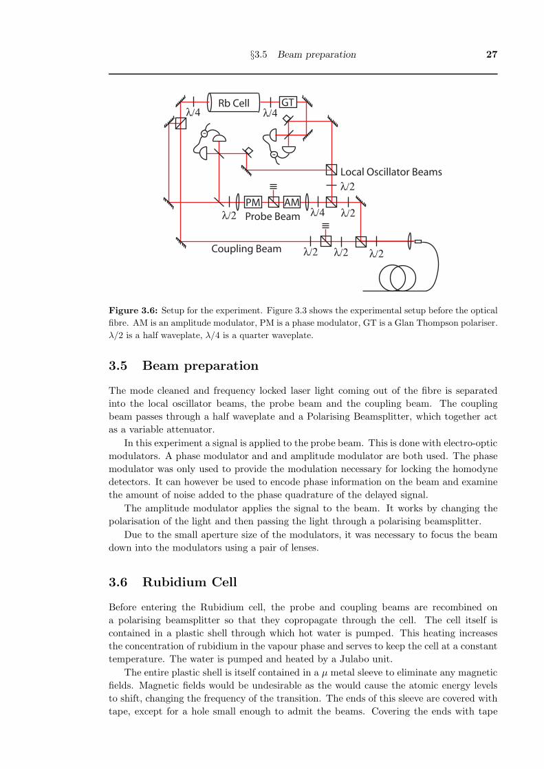
§3.5 Beam preparation 27

λ/2λ/2

λ/2λ/4AMPM

λ/2

-

λ/2

λ/4Rb Cell

λ/4GT

-

Coupling Beam

Probe Beam

Local Oscillator Beams

λ/2

Figure 3.6: Setup for the experiment. Figure 3.3 shows the experimental setup before the optical

fibre. AM is an amplitude modulator, PM is a phase modulator, GT is a Glan Thompson polariser.

λ/2 is a half waveplate, λ/4 is a quarter waveplate.

3.5 Beam preparation

The mode cleaned and frequency locked laser light coming out of the fibre is separated

into the local oscillator beams, the probe beam and the coupling beam. The coupling

beam passes through a half waveplate and a Polarising Beamsplitter, which together act

as a variable attenuator.

In this experiment a signal is applied to the probe beam. This is done with electro-optic

modulators. A phase modulator and and amplitude modulator are both used. The phase

modulator was only used to provide the modulation necessary for locking the homodyne

detectors. It can however be used to encode phase information on the beam and examine

the amount of noise added to the phase quadrature of the delayed signal.

The amplitude modulator applies the signal to the beam. It works by changing the

polarisation of the light and then passing the light through a polarising beamsplitter.

Due to the small aperture size of the modulators, it was necessary to focus the beam

down into the modulators using a pair of lenses.

3.6 Rubidium Cell

Before entering the Rubidium cell, the probe and coupling beams are recombined on

a polarising beamsplitter so that they copropagate through the cell. The cell itself is

contained in a plastic shell through which hot water is pumped. This heating increases

the concentration of rubidium in the vapour phase and serves to keep the cell at a constant

temperature. The water is pumped and heated by a Julabo unit.

The entire plastic shell is itself contained in a µ metal sleeve to eliminate any magnetic

fields. Magnetic fields would be undesirable as the would cause the atomic energy levels

to shift, changing the frequency of the transition. The ends of this sleeve are covered with

tape, except for a hole small enough to admit the beams. Covering the ends with tape

28 Experiment

serves to reduce thermal air currents caused by the hot cell.

Thermal convection causes major problems with the output homodyne due to the

varying phase shift caused by changes in refractive index in the hot and cold air.

Before the Rubidium cell, quarter waveplates rotate the probe and coupling beams into

orthogonal circular polarisations. After the Rubidium cell, a quarter waveplate restores

the coupling and probe beam to their original polarisations. The coupling beam is then

extinguished by a Glan Thompson polariser.

One problem associated with this setup is that the Coupling beam can undergo polar-

isation self-rotation [26] while passing through the atomic medium. This was checked for

in each experiment, always the amount of self-rotated Coupling Beam was less than the

amount of transmitted probe beam.

One proposed source of noise in the system is decoherence caused by atom-atom colli-

sions within the gas. To test this hypothesis, two cells where used. The first cell consisted

pure Rubidium-87. The second cell had a buffer gas added to the cell. The idea of a buffer

gas is that instead of colliding with other Rubidium atoms and decohereing, the Rubidium

atoms mostly collide with buffer gas atoms. The buffer gas is a noble gas that does not

cause a decoherence upon collision with Rubidium.

3.7 Homodyne Detectors

As outlined in the theory section, homodyne detectors can be adjusted to detect either

phase or quadrature. Experimentally, thermal and acoustic effects will change the phase

difference between the local oscillator beam and the signal beam. To keep this phase

difference constant, it is necessary to lock the homodyne detectors.

As given in the theory section, the subtraction of the photocurrent from the two

detectors in the homodyne detector is;

c†c − d†d = AB cos θ + 2AδXθb

When θ is zero, amplitude quadrature is being detected. When θ is π/2 phase quadra-

ture is being detected. The DC component of the signal is a maximum, so to lock to

amplitude quadrature involves locking to a maximum, similar to the laser frequency lock-

ing.

A modulation at 9.8MHz is applied to the phase modulator. This modulation is picked

up by the homodyne detector. The error signal is generated as described before and is

fed back into the piezoelectric crystal governing the phase of the local oscillator beam.

This mechanism ensures that the phase between the local oscillator and the input signal

remains constant and that the amplitude quadrature is always being detected.

As homodyne detectors rely on interference, it is necessary for the probe beam to have

the same mode and to have the same polarisation as the local oscillator. The polarisation

and mode-matching does not have to be perfect, the imperfections correspond to a reduced

visibility of the interference.

§3.8 Data Acquisition 29

3.8 Data Acquisition

3.8.1 Network Analyser

A network analyser is a device which outputs a swept sine wave. The model used was

a Anritsu MS4630B. This output signal is applied to some part of the experiment and

then a signal is fed back to the network analyser. The network analyser can calculate

the phase shift between these two signals and hence the delay. It is convenient because it

can take data on both the delay and transmission of the EIT as a function of frequency

very quickly. This speed makes it practical to take this data for a range of probe power

and coupling beam power values. This large amount of data makes it possible to build up

the contour plots of transmission and delay vs frequency and power shown in the results

section.

3.8.2 PXI

The PXI is a fast digital oscilloscope that can capture data on four channels. The model

used was a National Instruments PXI-1042. In this experiment I’ve only used two of those

channels, one for the input homodyne and the other for the output homodyne detector.

Data acquired through this system can be post processed to obtain information on delay,

attenuation and conditional variance. The advantage of this system over the Network

Analyser is that it can deliver a conditional variance measurement. As explained in the

theory section, this is the quantity used to infer added noise in the system.

A disadvantage of the PXI system is that is has a limited dynamic range. With only

8-bit analogue to digital converters, the number of values the digitisers can take is 28

which corresponds to a dynamic range of 24dB.

3.9 Data Processing

Data taken on the PXI needs to be processed before it can be usefully interpreted. Matlab

is used to analyse the data. It is theoretically possible to modulate the probe beam with

broadband noise and get all the required information from post-processing of this signal.

The noise could just be filtered at each frequency of interest and delay, attenuation and

conditional variance could then be calculated. This type of process would allow a broad

range of information to be inferred from one single shot measurement. However, it was

necessary to take data at discrete frequencies by modulating the probe beam at stepped

frequencies and taking data at each frequency. Single-shot measurement proved to be too

noisy due to limited amounts of data.

3.9.1 Delay measurement

To calculate the delay between the input and the output signals, data was filtered with

a gaussian filter at the frequency of interest. The filter serves to remove noise at any

frequencies other than the frequency of interest. Signals were then multiplied together in

the Fourier domain and then transformed back into the time domain. This is effectively

a convolution between two sine waves. The maximum of this convolution corresponds to

the time delay.

30 Experiment

Figure 3.7: Experimental Setup.

3.9.2 Normalisation to Quantum Noise

By blocking both the probe and coupling beams, only the local oscillator beams are in-

cident on the homodyne detectors. The two photodetectors in each homodyne setup are

balanced, so the subtraction of the two photocurrents gives the quantum noise. This noise

was recorded using the PXI to create a noise benchmark. The quantum noise data was

filtered with a gaussian filter at each frequency, then the variance was calculated at each

frequency. This was calculated for each homodyne. The resulting power vs frequency data

is used to normalise the measurements of the conditional variance.

3.9.3 Conditional Variance and Attenuation

The algorithm used to find the conditional variance and the attenuation comes from Equa-

tion 2.10. Data is first shifted by the calculated delay, then filtered with a Gaussian filter.

Data from each homodyne detector is then divided by the relevant quantum noise data

to get the correct normalistation. A minimisation procedure based on 2.10 then finds the

conditional variance, V1|2, and the corresponding attenuation, g.

Due to the difference between an ideal and a practical conditional variance measure-

ment, a factor of 2g2 must be subtracted. The reasons for this are explained in section

2.4.

Chapter 4

Results

4.1 Laser Noise

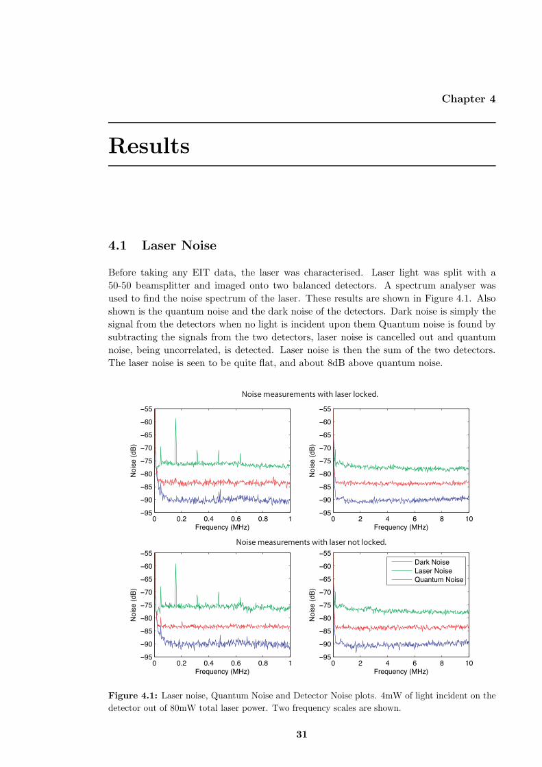
Before taking any EIT data, the laser was characterised. Laser light was split with a

50-50 beamsplitter and imaged onto two balanced detectors. A spectrum analyser was

used to find the noise spectrum of the laser. These results are shown in Figure 4.1. Also

shown is the quantum noise and the dark noise of the detectors. Dark noise is simply the

signal from the detectors when no light is incident upon them Quantum noise is found by

subtracting the signals from the two detectors, laser noise is cancelled out and quantum

noise, being uncorrelated, is detected. Laser noise is then the sum of the two detectors.

The laser noise is seen to be quite flat, and about 8dB above quantum noise.

0 0.2 0.4 0.6 0.8 1−95

−90

−85

−80

−75

−70

−65

−60

−55

Frequency (MHz)

No

ise

(d

B)

0 2 4 6 8 10−95

−90

−85

−80

−75

−70

−65

−60

−55

Frequency (MHz)

No

ise

(d

B)

0 0.2 0.4 0.6 0.8 1−95

−90

−85

−80

−75

−70

−65

−60

−55

Frequency (MHz)

No

ise

(d

B)

0 2 4 6 8 10−95

−90

−85

−80

−75

−70

−65

−60

−55

Frequency (MHz)

No

ise

(d

B)

Dark Noise

Laser Noise

Quantum Noise

Noise measurements with laser locked.

Noise measurements with laser not locked.

Figure 4.1: Laser noise, Quantum Noise and Detector Noise plots. 4mW of light incident on the

detector out of 80mW total laser power. Two frequency scales are shown.

31

32 Results

Coupling beam power (mW)

Fre

quen

cy o

f mod

ulat

ion

(Hz)

Transmission of Signal with 50µW Probe Beam (dB)

−55

−50 −45−40 −35 −30

−25

−20

−150 5 10 15 20 25

0.5

1

1.5

2

2.5x 10

5

−60

−50

−40

−30

−20

−10


Fre

quen

cy o

f mod

ulat

ion

(Hz)

Delay of Signal with 50µW Probe Beam(µs)

4.55

5.5

66.578

7

0 5 10 15 20 25

0.5

1

1.5

2

2.5x 10

5

0

2

4

6

8

Figure 4.2: Delay and Transmission for an unbuffered Rubidium Cell. 50µW Probe beam.

4.2 Delay Measurements

By using the network analyser plots of delay vs. frequency and plots of attenuation vs.

frequency can be generated very quickly. By taking this data for multiple values of the

coupling beam strength, it was possible to build up a contour plot showing the parameters

that correspond to the best delay. All data was taken with the Rubidium cell heated to

58oC.

4.2.1 Unbuffered Rubidium Cell

Using an isotopically purified Rubidium-87 vapour cell, delay and transmission where

measured as a function of frequency and coupling beam power for three different Probe

beam powers. These results are displayed in Figures 4.2, 4.3, 4.4.

Universally these plots show that with increasing frequency of modulation, the delay

time decreases and the transmission decreases. This is consistent with the fact the EIT has

a limited bandwidth. On all three plots the maximum delay occurs when the frequency

of modulation and coupling power are both very small. This is, however, not useful

because this region also corresponds to a minimum in transmission. A local maximum in

delay also occurs for moderate coupling beam strengths with small modulation frequency.

These local maxima in delay time corresponds to reasonable signal transmissions and so

constitute a useful result.

These local maxima make sense. An increase in coupling beam strength would lead

to a broadening of the transparency bandwidth. This would mean the susceptibilitiy

gradient would be shallower, corresponding to a smaller delay time. On the other hand,

as the coupling beam gets smaller, the bandwidth of transparency gets smaller and starts

§4.2 Delay Measurements 33


Fre

quen

cy o

f mod

ulat

ion

(Hz)


−55−50

−45 −40 −35−30 −25 −20−15

0 5 10 15 20 25

1

2

3

4x 10

5

−60

−50

−40

−30

−20

−10

0


Fre

quen

cy o

f mod

ulat

ion

(Hz)


3

3.544.5

55.5

66.5

0 5 10 15 20 25

0.5

1

1.5

2

2.5

3

3.5

4x 10

5

0

2

4

6

8



Fre

quen

cy o

f mod

ulat

ion

(Hz)


−50

−45−40 −35 −30 −25

−20−15

0 5 10 15 20

0.5

1

1.5

2

2.5

3x 10

5

−60

−50

−40

−30

−20

−10

0


Fre

quen

cy o

f mod

ulat

ion

(Hz)


44.5

5

5.566.577.58

0 5 10 15 20

0.5

1

1.5

2

2.5

3x 10

5

0

2

4

6

8

10


34 Results


Fre

quen

cy o

f mod

ulat

ion

(Hz)


−24

−22

−20 −18−16 −14

−12−10

0 5 10 15 20 25 30

0.5

1

1.5

2

2.5x 10

5

−25

−20

−15

−10


Fre

quen

cy o

f mod

ulat

ion

(Hz)


0.5

1

1.522.5

0 5 10 15 20 25 30

0.5

1

1.5

2

2.5x 10

5

0

0.5

1

1.5

2

2.5

3

Figure 4.5: Delay and Transmission for a buffered Rubidium Cell. 200µW Probe beam.

to attenuate light at the sideband frequencies.

Importantly, 8µs delay is observed in Figure 4.4 at a modulation frequency of 50kHz.

As 50kHz corresponds to a period of 20µs, the 8µs satisfies the criteria of the delay time

being greater than one quarter of a period of the modulation given by [22]. This means

that the delay cannot be explained by saturable absorption effects.

4.2.2 Buffered Rubidium Cell

Isotopically pure Rubidium-87 and a buffer gas are mixed together in a vapour cell. Delay

and Transmission where measured as a function of frequency and coupling beam power.

These results are displayed in Figures 4.5, 4.6, 4.7. Data was also taken for 100µW probe

beam, however signal was too low and the data was too noisy to be useful. It should be

noted that the beam sizes of the probe and coupling beams where changed between the

measurements for the buffered and unbuffered cells. As such, it is not useful to compare

the power of the probe beam between the buffered and unbuffered cells.

The buffered cell shows no maximum in delay for small coupling power and small

modulation frequency. Also, there seems to be no local maximum of delay time, with

delay increasing for lower modulation frequencies. Other than these differences, the data

is qualitatively similar to that of the unbuffered cell.

The maximum delay achieved for this cell is lower than that of the unbuffered cell.

Also the overall amount of attenuation is less. Both of these effects are due to the fact

that the two types of cell are operating at the same temperature, however the buffer gas

cell has the buffer gas present, which takes a partial pressure. This allows less Rubidium

into the vapour phase and so the number of atoms that the beam addresses is smaller.

Equation 2.3, 2.5, 2.6 and 2.8 show that an decrease in N leads to an increase in the group

§4.2 Delay Measurements 35


Fre

quen

cy o

f mod

ulat

ion

(Hz)


−40

−35−30

−25

−20

0 5 10 15 20 25

0.5

1

1.5

2

2.5x 10

5

−60

−50

−40

−30

−20

−10


Fre

quen

cy o

f mod

ulat

ion

(Hz)


4.5 43.5 32.5

21.5

10.5

0 5 10 15 20 25

0.5

1

1.5

2

2.5x 10

5

0

1

2

3

4

5



Fre

quen

cy o

f mod

ulat

ion

(Hz)


−30−27 −24 −21

−18−15

−120 5 10 15 20

0.5

1

1.5

2

2.5x 10

5

−60

−50

−40

−30

−20


Fre

quen

cy o

f mod

ulat

ion

(Hz)


0.51

1.5

22.5

33.54

0 5 10 15 20

0.5

1

1.5

2

2.5x 10

5

0

1

2

3

4

5


36 Results

velocity.

4.2.3 Spatial Effects

One of the non-quantitative results to come from these experiments is that EIT has a large

dependance on spatial effects. Mode quality, beam alignment and the size ratio between

pump and probe all had an effect on the quality of the delay achieved.

In fact, for some configurations, transmission was actually worsened by the application

of the coupling beam. We believe this particular effect was caused by having the probe and

coupling beam misaligned, or having the coupling beam much larger than the probe beam.

This would mean that the coupling and probe beams would be operating in different spatial

regions of the cell, and so the could not produce EIT. The separate regions, however, would

still be coupled by the thermal drift of the atoms and so optical pumping could still occur.

Given the need to constantly adjust for thermal drift in the optical components, the

beam configuration would not have been the same for both cells.

The buffered Rubidium cell did not have very flat optical surfaces, resulting in mode

shape distortion after passage through the cell. This resulted in lower fringe visibility in

the output homodyne detector.

Further it was necessary to tilt the cells slightly to avoid back reflections from the

uncoated glass faces of the cells.

4.3 PXI Measurements and Post Processing

To characterise the extra noise added to the beam by EIT it is necessary to use the PXI.

The PXI saves raw data, from which it is possible to calculate the conditional variance,

which is a measure of noise. Before calculating the variance however it is necessary to

calculate the delay. These calculations are done via the methods described in section 3.9.

All of the data shown in this section was taken with a coupling beam strength of

2.5mW, and a probe strength of 200µW. The area of the coupling beam was approximately

3.5 times greater than that of the probe.

4.3.1 Noise Characteristics of the Measurement System

Figure 4.8 shows the noise measurements of the system taken with a homodyne detector.

The PXI noise is calculated by unplugging the detectors from the PXI.

The noise of the detectors is calculated by blocking all laser light from hitting the

detectors. The peaks in the detector noise are not expected. It can clearly be seen that

the detector noise peaks affects the measurement of quantum noise and even laser noise.

The noise peaks shown in the detector noise are a big problem as they do not show up in

the earlier measurement done with the spectrum analyser, results of which are shown in

Figure 4.1. A more recent check of detector noise was made with the network analyser,

which also showed a flat noise spectrum. This suggests that the peaks are most likely due

to something in either the PXI or in the data processing methods. Experiments using the

PXI should be repeated to see if these noise peaks are repeatable.

Quantum noise is calculated by putting the local oscillator beam into the homodyne

detector. Any noise on the laser beam is detected equally by both detectors and is sub-

tracted away, the only source of noise left in the detector signal is the quantum noise

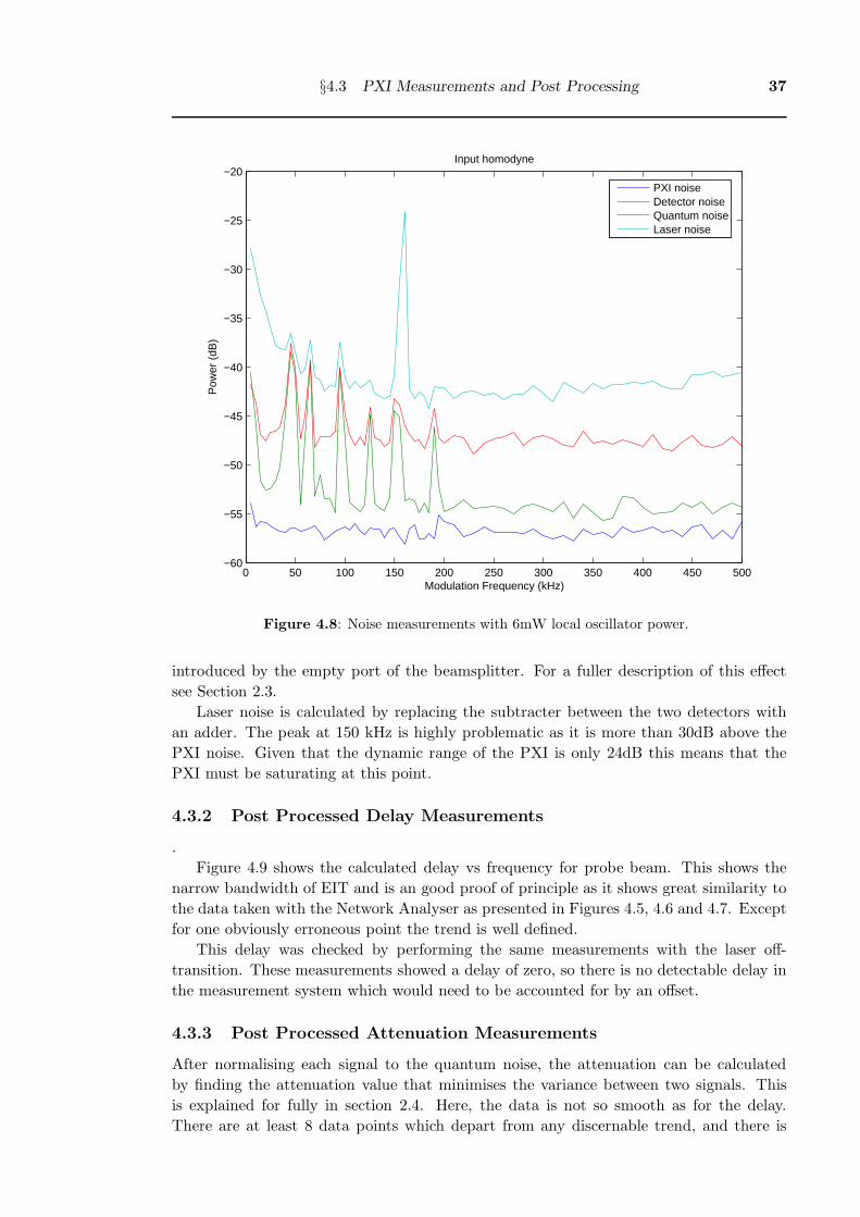
§4.3 PXI Measurements and Post Processing 37

0 50 100 150 200 250 300 350 400 450 500−60

−55

−50

−45

−40

−35

−30

−25

−20

Modulation Frequency (kHz)

Pow

er (

dB)

Input homodyne

PXI noiseDetector noiseQuantum noiseLaser noise

Figure 4.8: Noise measurements with 6mW local oscillator power.

introduced by the empty port of the beamsplitter. For a fuller description of this effect

see Section 2.3.

Laser noise is calculated by replacing the subtracter between the two detectors with

an adder. The peak at 150 kHz is highly problematic as it is more than 30dB above the

PXI noise. Given that the dynamic range of the PXI is only 24dB this means that the

PXI must be saturating at this point.

4.3.2 Post Processed Delay Measurements

.

Figure 4.9 shows the calculated delay vs frequency for probe beam. This shows the

narrow bandwidth of EIT and is an good proof of principle as it shows great similarity to

the data taken with the Network Analyser as presented in Figures 4.5, 4.6 and 4.7. Except

for one obviously erroneous point the trend is well defined.

This delay was checked by performing the same measurements with the laser off-

transition. These measurements showed a delay of zero, so there is no detectable delay in

the measurement system which would need to be accounted for by an offset.

4.3.3 Post Processed Attenuation Measurements

After normalising each signal to the quantum noise, the attenuation can be calculated

by finding the attenuation value that minimises the variance between two signals. This

is explained for fully in section 2.4. Here, the data is not so smooth as for the delay.

There are at least 8 data points which depart from any discernable trend, and there is

38 Results

0 50 100 150 200 250 300 350 400 450 5000

0.5

1

1.5

2

2.5

3

3.5

4


Del

ay T

ime

(µ s

)

Delay Time vs Modulation Frequency for Buffer Gas Cell.

Figure 4.9: Delay versus modulation frequency for the Buffer Gas cell.

an inexplicable rise in transmission at between 300kHz and 350kHz. Finally, the signal to

noise ratio for the plot is disappointingly low. Given that over 100,000 points of data where

taken with the PXI, enough detail should be present to determine the gain with greater

accuracy than this. When the inaccuracy on these measurements are compared to the

smooth contour plots generated by the network analyser, the PXI is disappointing. Other

than that, the data looks as expected, showing a drop in transmission with increasing

modulation frequency.

4.3.4 Conditional Variance

The Conditional Variance is the most troubling result of all. Values in the thousands do

not agree with Hsu’s earlier work [17]. In fact they are hundreds of times larger than Hsu’s

results. One potential source of this problem is an error in the normalisation part of the

algorithm described in Section 3.9.

To check for this error, I resubstituted the Quantum Noise data back into the Con-

ditional Variance algorithm to check that the normalisation code was working correctly.

Figure 4.12 shows the results of this test, and it shows that in the main part, the nor-

malisation is correct, or at least not incorrect enough to account for the huge size of the

Conditional Variance.

This leaves the process itself or the PXI as explanations for the exceptional values of

the conditional variance. To properly narrow down the error, more data needs to be taken

to see if the errors are repeatable.

Hsu’s method of calculating the conditional variance was entirely electronic. Delay

§4.3 PXI Measurements and Post Processing 39

0 50 100 150 200 250 300 350 400 450 50010

20

30

40

50

60

70

80

90

100


Sig

nal T

rans

mis

sion

(%

)

Bandwidth of EIT

Figure 4.10: Gain calculated using post-processed PXI data.

was manually adjusted by varying the length of a BNC cable and the gain was manually

adjusted to minimise the correlation between the input and output homodynes. The main

advantage the PXI method has is that it is much faster. Even when modulating at discrete

frequencies the data taking process is much faster. Unfortunately difficulty analysing the

data prevented further data being taken.

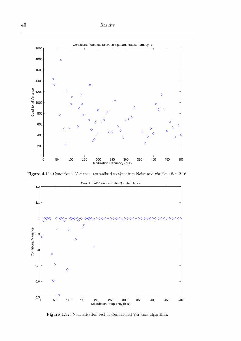
40 Results

0 50 100 150 200 250 300 350 400 450 5000

200

400

600

800

1000

1200

1400

1600

1800

2000


Con

ditio

nal V

aria

nce

Conditional Variance between input and output homodyne

Figure 4.11: Conditional Variance, normalised to Quantum Noise and via Equation 2.16

0 50 100 150 200 250 300 350 400 450 5000.5

0.6

0.7

0.8

0.9

1

1.1

1.2


Con

ditio

nal V

aria

nce

Conditional Variance of the Quantum Noise

Figure 4.12: Normalisation test of Conditional Variance algorithm.

Chapter 5

Conclusion and Future Directions

5.1 Conclusions

In this thesis, experiments have been done to build up a comprehensive characterisation

of EIT signal delay and transmision as a function of modulation frequency and coupling

beam power. This same method can be used with future EIT systems to find points of

optimal delay, transmission and bandwidth.

Furthermore these results show that for cells at equal temperature, better delay can

be achieved with an unbuffered cell. However, for a better comparison, the cells should

be compared with equal atomic densities since the buffered cell will have a lower atomic

density due to the presence of the buffer gas.

Attempts at making single-shot measurements to determine delay, transmission and

added noise have shown that more work needs to be done to properly understand the

methodology. In order to verify the noise results obtained, more measurements need to be

made.1

5.2 Future Directions

Future experiments should focus on understanding the PXI system and how to do single-

shot measurements of the amount of excess noise in an EIT system. Problems to be solved

include fitting all modulations inside the dynamic range of the PXI. Also the algorithms

for post processing the data can be investigated. Gaussian filters and top hat filters where

chosen for their simplicity although more optimal filter shapes may well exist.

Also, the high dependance on spatial effects could be investigated in more detail. In

particular the hypothesis that coupling and probe beams can effect each other via the

thermal drift of the atoms should be tested. Some work has already been done in this area

[27, 28, 29].

1I will be working on verification of these results over the next few months as we will possibly be

preparing a manuscript for publication.

41

42 Conclusion and Future Directions

Bibliography

[1] G. Alzetta, A. Gozzini, L. Moi, and G. Orriols. An experimental method for the

observation of r.f. transitions and laser beat resonances in oriented Sodium Vapour.

Nuovo Cimento B, 36:5, 1976.

[2] S. E. Harris. Electromagnetically induced transparency. Physics Today, 50:36–42,

July 1997.

[3] K.-J. Boller, A. Imamolu, and S. E. Harris. Observation of electromagnetically in-

duced transparency. Phys. Rev. Lett., 66(20):2593–2596, May 1991.

[4] L. V. Hau, S. E. Harris, Z. Dutton, and C. H. Behroozi. Light speed reduction to 17

metres per second in an ultracold atomic gas. Nature, 397:594–598, 1999.

[5] D. F. Phillips, A. Fleischhauer, A. Mair, R. L. Walsworth, and M. D. Lukin. Storage

of light in atomic vapor. Phys. Rev. Lett., 86(5):783–786, Jan 2001.

[6] M. Bajcsy, A. S. Zibrov, and M. D. Lukin. Stationary pulses of light in an atomic

medium. Nature, 426:638–641, 2003.

[7] C. Liu, Z. Dutton, C. H. Behroozi, and L. V. Hau. Observation of coherent optical

information storage in an atomic medium using halted light pulses. Nature, 409:490–

493, 2001.

[8] A. V. Turukhin, V. S. Sudarshanam, M. S. Shahriar, J. A. Musser, B. S. Ham, and

P. R. Hemmer. Observation of ultraslow and stored light pulses in a solid. Phys. Rev.

Lett., 88(2):023602, Dec 2001.

[9] J. J. Longdell, E. Fraval, M. J. Sellars, and N. B. Manson. Stopped light with storage

times greater than one second using electromagnetically induced transparency in a

solid. Phys. Rev. Lett., 95(6):063601, 2005.

[10] T. Chaneliere, D. N. Matsukevich, S. D. Jenkins, S.-Y. Lan, T. A. B. Kennedy, and

A. Kuzmich. Storage and retrieval of single photons transmitted between remote

quantum memories. Nature, 438:833–836, December 2005.

[11] M. M. Kash, V. A. Sautenkov, A. S. Zibrov, L. Hollberg, G. R. Welch, M. D. Lukin,

Y. Rostovtsev, E. S. Fry, and M. O. Scully. Ultraslow group velocity and enhanced

nonlinear optical effects in a coherently driven hot atomic gas. Phys. Rev. Lett.,

82(26):5229–5232, Jun 1999.

[12] M. Fleischhauer and M. D. Lukin. Dark-state polaritons in electromagnetically in-

duced transparency. Phys. Rev. Lett., 84(22):5094–5097, May 2000.

[13] A. Dantan and M. Pinard. Quantum-state transfer between fields and atoms in

electromagnetically induced transparency. Physical Review A (Atomic, Molecular,

and Optical Physics), 69(4):043810–+, April 2004.

43

44 Bibliography

[14] A. B. Matsko, Y. V. Rostovtsev, O. Kocharovskaya, A. S. Zibrov, and M. O. Scully.

Nonadiabatic approach to quantum optical information storage. Phys. Rev. A,

64(4):043809, Sep 2001.

[15] A. Peng, M. Johnsson, W. P. Bowen, P. K. Lam, A. Bachor, H, and J. J. Hope.

Squeezing and entanglement delay using slow light. Physical Review A (Atomic,

Molecular, and Optical Physics), 71(3):033809, 2005.

[16] D. Akamatsu, K. Akiba, and M. Kozuma. Electromagnetically induced transparency

with squeezed vacuum. Phys. Rev. Lett., 92(20):203602, 2004.

[17] M. T. Hsu, G. Hetet, O. Glockl, J. J. Longdell, B. C. Buchler, H.-A. Bachor, and

P. K. Lam. Quantum study of information delay in electromagnetically induced

transparency. Phys. Rev. Lett., Accepted for Publication, 2006.

[18] A. B. Matsko, I. Novikova, M. O. Scully, and G. R. Welch. Radiation trapping in

coherent media. Phys. Rev. Lett., 87(13):133601, Sep 2001.

[19] E. B. Aleksandrov and V. S. Zapasskii. A fairy tale of stopped light. Physics Uspekhi,

47:1033–1036, 2004.

[20] E. B. Aleksandrov and V. S. Zapasskii. Chasing ’Slow Light’. ArXiv Physics e-prints,

February 2006.

[21] A. M. Akulshin, A. Lezama, A. I. Sidorov, R. J. McLean, and P. Hannaford. ’Storage

of light’ in an atomic medium using electromagnetically induced absorption. Journal

of Physics B Atomic Molecular Physics, 38:L365–L374, December 2005.

[22] A. C. Selden. Saturable absorption and ’slow light’. ArXiv Physics e-prints, Decem-

ber 2005.

[23] A. Peng. Atom-Light Interactions in Electromagnetically Induced Transparency.

Master’s thesis, Australian National University, February 2005.

[24] D. A. Steck. Rubidium 87 D Line Data. http://steck.us/alkalidata/, September 2001.

[25] C. J. Foot. Atomic Physics. Oxford Masters Series in Physics. Oxford University

Press, 2005.

[26] M. T. Hsu, G. Hetet, A. Peng, C. C. Harb, H.-A. Bachor, M. T. Johnsson, J. J. Hope,

P. K. Lam, A. Dantan, J. Cviklinski, A. Bramati, and M. Pinard. Effect of atomic

noise on optical squeezing via polarization self-rotation in a thermal vapor cell. Phys.

Rev. A, 73(2):023806, February 2006.

[27] Jing Cheng, Shensheng Han, and YiJing Yan. Transverse localization and slow

propagation of light. Physical Review A (Atomic, Molecular, and Optical Physics),

72(2):021801, 2005.

[28] Jing Cheng and Shensheng Han. Manipulating spectral anomalies of focused pulses

in a medium with electromagnetically induced transparency. Physical Review A

(Atomic, Molecular, and Optical Physics), 73(6):063803, 2006.

Bibliography 45

[29] Richard R. Moseley, Sara Shepherd, David J. Fulton, Bruce D. Sinclair, and Mal-

colm H. Dunn. Spatial consequences of electromagnetically induced transparency:

Observation of electromagnetically induced focusing. Phys. Rev. Lett., 74(5):670–

673, Jan 1995.

attenuation, delay and noise properties of light slowed by

Documents