atmospheric models of transport and …acmg.seas.harvard.edu/education/brasseur_jacob/ch11_bra...guy...
TRANSCRIPT
Guy P. Brasseur and Daniel J. Jacob, Mathematical Modeling of Atmospheric Chemistry Chapter 11, October 2013 draft
© by G.P. Brasseur and D.J. Jacob, all rights reserved Page 1
11.
Inverse Modeling
11.1 Introduction
Inverse modeling is a formal approach for estimating the values of the variables driving the evolution of a system by taking measurements of the observable manifestations of that system, and using our physical understanding to relate these observations to the driving variables. We call the variables that we wish to estimate the state variables, and assemble them into a state vector x. We similarly assemble the observations into an observation vector y. Our understanding of the relationship between x and y is described by a physical model F, called the forward model:
( , )=y F x p + ε (11.1)
where p is a parameter vector including all model variables that we do not seek to optimize (we call them model parameters), and ε is an error vector including contributions from errors in the observations, in the forward model, and in the model parameters. From inversion of equation (11.1), we can obtain x given y. In the presence of error ( ≠ε 0 ), the best that we can achieve is a statistical estimate, and we need to weigh the resulting information against our prior (a priori) knowledge xA of the state vector before the observations were made. The optimal solution of x reflecting this ensemble of constraints is called the a posteriori, the maximum a posteriori (MAP), the optimal estimate, or the retrieval. We will use these terms interchangeably, with some preference for optimal estimate which is the more general terminology. Retrieval is the standard terminology for remote sensing. The choice of state vector (i.e., which variables to include in x vs. in p) is up to us. It depends on what variables we wish to optimize, what information is contained in the observations, and what computational costs are associated with the inversion. Inverse modeling has three major types of applications in atmospheric chemistry (Table 11.1):

Guy P. Brasseur and Daniel J. Jacob, Mathematical Modeling of Atmospheric Chemistry Chapter 11, October 2013 draft
© by G.P. Brasseur and D.J. Jacob, all rights reserved Page 2
Table 11.1 Applications of inverse modeling to atmospheric chemistry problems
Application type State vector Observation vector
Forward model A priori
Remote sensing Vertical concentration profile
Wavelength-dependent radiances
Radiative transfer model
Climatological profile
Optimizing surface fluxes
Surface fluxes Atmospheric concentrations
CTM Bottom-up inventory
Data assimilation (3DVAR)
Gridded concentration field (to)
Atmospheric concentrations at to
Mapping from observations to CTM grid
Forecast
Data assimilation (4DVAR)
Gridded concentration field (to)
Atmospheric concentrations over [to+∆t]
Forecast model Forecast
1. Retrieval of atmospheric concentrations from observed radiances. Consider the problem of using radiance spectra measured by remote sensing to retrieve vertical concentration profiles of a trace species. The measured radiances at different wavelengths represent the observation vector y, and the concentrations at different vertical levels represent the state vector x. The forward model is a radiative transfer model that solves the radiative transfer equation to calculate y as a function of x and of additional parameters p including surface emissivity, temperatures, clouds, spectroscopic data, etc. Inversion of this forward model using the observed spectra then provides a retrieval of x.
2. Optimal estimation of surface fluxes. Consider the problem of quantifying surface fluxes of a species on a (latitude x longitude x time) grid. The fluxes on that grid represent the state vector x. We measure atmospheric concentrations of the species or related species (such as reaction products) and assemble these data into an observation vector y. The forward model is a CTM that solves the continuity equation to calculate y

Guy P. Brasseur and Daniel J. Jacob, Mathematical Modeling of Atmospheric Chemistry Chapter 11, October 2013 draft
© by G.P. Brasseur and D.J. Jacob, all rights reserved Page 3
as a function of x. The parameter vector p includes meteorological variables, and may also include chemical variables (such as rate constants) and any characteristics of the surface flux (such as diurnal variability) that are simulated in the CTM but not optimized through the state vector. The information on x from the observations is called a top-down constraint on the surface fluxes. A priori information on x based on our knowledge of the processes determining the surface fluxes (such as fuel combustion statistics, land cover data bases, etc) is called a bottom-up constraint. Combination of the top-down and bottom-up constraints provides an optimal estimate for x. Instead of the surface fluxes themselves, we may wish to optimize the driving variables of a surface flux model; the approach is exactly the same but the dimension of x may be advantageously reduced.
3. Data assimilation. Consider the problem of constructing a continuous and evolving gridded 3-D field of concentrations x(t) on the basis of measurements y made at various locations and times. Such a construction may be useful to assist weather forecasts, to initialize chemical forecasts, to assess the consistency of measurements made from different platforms, or to improve estimates of the concentrations of non-measured species from measurements of chemically linked species. We refer to this class of inverse modeling problems as data assimilation. An essential component is a forecast model that projects the evolution of concentrations over a forecasting time interval from t0 to t0 + h. This forecast model can be as simple as a persistence model (x(t0 + h) = x(t0)) or as complex as a full meteorological model enabling consistent meteorological and chemical data assimilation. In the Kalman filter (also called 3DVAR), observed concentrations of the species to be optimized are collected and assimilated at fixed time intervals h (such as daily). Thus the observations y(to) at time to are used to optimize x(to), where the forward model is simply a mapping of the observations onto the 3-D grid. We then use the forecast model over the time interval [to, to+h] to obtain an a priori for x(to+h), apply the observations at time to+h to optimize x(to+h), and so on. In variational data assimilation (also called 4DVAR), the ensemble of observations spread over the time interval [to, to+h] are used to optimize x(to) by applying the adjoint of the forecast model backward in time over [to+h, to]. The forecast model is then used to obtain an a priori for x(to+h), observations over [to+h, to+2h] are used to optimize x(to+h), and so on.
Proper consideration of errors is crucial in inverse modeling. To appreciate this, let us examine what happens if we ignore errors. We linearize the forward model y = F(x, p) around the a priori estimate xA taken as first guess:
2( , ) ( ) (( ) )= + − + −A A Ay F x p K x x Ο x x (11.2)
Guy P. Brasseur and Daniel J. Jacob, Mathematical Modeling of Atmospheric Chemistry Chapter 11, October 2013 draft
© by G.P. Brasseur and D.J. Jacob, all rights reserved Page 4
where /= ∂ ∂K y x is the Jacobian matrix of the forward model with elements /ij i jk y x= ∂ ∂ evaluated at x = xA. Let n and m be the dimensions of x and y, respectively. In the
absence of error, m = n independent measurements constrain x uniquely. The Jacobian matrix is then a nxn matrix of full rank and hence invertible. We obtain for x:
( ( , ))−= + −1A Ax x K y F x p (11.3)
If F is nonlinear, the solution (11.3) must be iterated with recalculation of the Jacobian at successive guesses for x until satisfactory convergence is achieved.
Now what happens if we make additional observations, such that m > n? In the absence of error these observations must necessarily be redundant. However, we know from experience that useful constraints on an atmospheric system typically require a very large number of measurements, m >> n. This reflects errors in the observations and in the forward model, described by the error vector ε in equation (11.1). Thus equation (11.3) is not applicable in practice; successful inversion requires adequate characterization of the error and consideration of a priori information on x. The a priori estimate has its own error:
A Ax = x + ε (11.4)
and the inverse problem then involves weighting the error statistics of ε and εA to solve the optimal estimation problem, “what is the best estimate of x given y?”. This is done using Bayes’ theorem, as described below.
11.2 Bayes’ Theorem
Bayes’ theorem provides the general foundation for most inverse models. Consider a pair of vectors x and y. Let P(x), P(y), P(x,y) represent the corresponding probability distribution functions (pdfs), so that the probability of x being in the range [x, x+dx] is P(x)dx, the probability of y being in the range [y, y+dy] is P(y)dy, and the probability of (x, y) being in the range ([x, x+dx], [y, y+dy]) is P(x,y)dxdy. Let P(y|x) represent the pdf of y when x has a certain value. We can write P(x,y)dxdy equivalently as
( ) ( ) ( )P d d P d P d=x,y x y x x y x y (11.5)
or as

Guy P. Brasseur and Daniel J. Jacob, Mathematical Modeling of Atmospheric Chemistry Chapter 11, October 2013 draft
© by G.P. Brasseur and D.J. Jacob, all rights reserved Page 5
( ) ( ) ( )P d d P d P d=x,y x y y y x y x (11.6)
Eliminating P(x,y), we obtain Bayes’ theorem:
( ) ( )( )( )
P PPP
=y | x xx | y
y (11.7)
This theorem formalizes the inverse problem posed in section 11.1. Here P(x) is the pdf of the state vector x before the measurements are made (that is, the a priori pdf). P(y|x) is the pdf of the observation vector y given the true value for x. P(x|y) is the a posteriori pdf for the state vector reflecting the information from the measurements – that is, it is the pdf of x given the measurements y. The optimal solution for x is given by the maximum of P(x|y), that is, the solution to ( | )P∇ =x x y 0 where ∇x is the gradient operator in the state vector space. The probability function P(y) in the denominator of (11.7) is independent of x, and we can view it merely as a normalizing factor to ensure that
0
( | ) 1P∞
=∫ x y dx (11.8)
It plays no role in determining the MAP solution (since it is independent of x) and we ignore it in what follows.
11.3 A Simple Scalar Example
Application of Bayes’ theorem to solve the inverse problem can be easily understood with a simple example using scalars. This allows us to introduce terminology and equations that will be central to understand the solution of the more general problem involving vectors. Consider in this example a single source releasing a species X to the atmosphere with an emission rate x (Figure 11.1). We have an a priori estimate A Ax σ± for the value of x, where σA
2 is the error variance on that estimate. For example, if X is emitted from a combustion source, the a priori information could be a bottom-up emission estimate based on knowledge of the type and amount of fuel being burned, the combustion regime, any emission control equipment, etc. We now set up a sampling site to measure the concentration of X downwind of the source. We make a single measurement y = y’ + εI, where y’ is the true concentration and εI, is the instrument error. We then use a CTM as forward model F to relate y’ to x:

Guy P. Brasseur and Daniel J. Jacob, Mathematical Modeling of Atmospheric Chemistry Chapter 11, October 2013 draft
© by G.P. Brasseur and D.J. Jacob, all rights reserved Page 6
' ( ) M Ry F x ε ε= + + (11.9) where εM describes the CTM error in reproducing the true concentration y’ given the true emission rate x. This error includes contributions from model parameters (such as assumed winds and chemistry), model physics, and model numerics. There is in addition a representation error εR reflecting the mismatch between the spatial and temporal resolution of the model and the precise location and time of the measurement (Figure 11.2).
Figure 11.1 Simple inverse modeling application. A point source emits a species X with an estimated a priori emission rate xA. We seek to improve this estimate by measuring the concentration y of X at a point downwind, and using a CTM as forward model to relate x to y.
Figure 11.2 Representation error. The CTM computes concentrations y as gridbox averages over discrete time steps ∆t. The measurement is at a specific location and at a time t’ that does not correspond to the discrete model time steps. Interpolation in space and time is necessary to compare the measurement to the model, and the associated error is called the representation error. Representation error is not intrinsically a model error; it would not exist if the measurement were made as an average over the gridbox domain and at a time corresponding to a model time step. The measured concentration y is thus related to the true emission rate x by
( ) ( )I R M Oy F x F xε ε ε ε= + + + = + (11.10)

Guy P. Brasseur and Daniel J. Jacob, Mathematical Modeling of Atmospheric Chemistry Chapter 11, October 2013 draft
© by G.P. Brasseur and D.J. Jacob, all rights reserved Page 7
where εO = εI + εR + εM is the observational error which sums the instrument, representation, and forward model errors. This terminology might at first seem strange, as we are used to opposing observations to models. A very important conceptual point here is that instrument and model errors are inherently coupled in attempting to estimate x from y. Having a very precise instrument is useless if the model is poor or mismatched; in turn, having a very precise model is useless if the instrument is poor. Instrument and model must be viewed as inseparable partners of the observing system by which we seek to gain knowledge of x. The error variance σ2 is defined by:
( )22 [ [ ] ]E Eσ ε ε= − (11.11) where E[] is the expected value operator representing the average value of the bracketed quantity. The instrument, representation, and model errors are uncorrelated so that the variances are additive:
2 2 2 2O I R Mσ σ σ σ= + + (11.12)
Let us assume for now that the mean bias [ ]b E ε= is zero for both the instrument and the model; we will examine the implications of b ≠ 0 later. Let us further assume that all errors are normally distributed. Finally, let us assume that the forward model is linear so that F(x) = kx where k is the model parameter; again, we will examine the implications of non-linearity later. We now have all the elements needed for application of Bayes’ theorem to obtain an optimal estimate x for x given y. The a priori pdf for x is given by
2
2
( )1( ) exp[ ]22
A
AA
x xP xσσ π
−= − (11.13)
and the pdf for the observation y given the true value of x is given by
2
2
1 ( )( | ) exp[ ]22 OO
y kxP y xσσ π
−= − (11.14)
as follows from equation (11.10). Applying Bayes’ theorem (11.7) and ignoring the normalizing terms that are independent of x, we obtain:
Guy P. Brasseur and Daniel J. Jacob, Mathematical Modeling of Atmospheric Chemistry Chapter 11, October 2013 draft
© by G.P. Brasseur and D.J. Jacob, all rights reserved Page 8
2 2
2 2
( ) ( )( | ) exp[ ]2 2
A
A O
x x y kxP x yσ σ
− −∝ − − (11.15)
where ∝ is the proportionality symbol. Finding the maximum value for P(x|y) is equivalent to finding the minimum for the cost function J(x):
2 2
2 2
( ) ( )( ) A
A O
x x y kxJ xσ σ− −
= + (11.16)
which is a least-squares cost function weighted by the variance of the error in the individual terms. It is called a χ2 cost function, and J(x) as formulated in equation (11.16) is called the χ2 statistic.
The optimal estimate x is the solution to / 0J x∂ ∂ = , which is straightforward to obtain analytically from (11.16):
ˆ ( )A Ax x g y kx= + − (11.17)
where g is a gain factor given by
2
2 2 2A
A O
kgk
σσ σ
=+
(11.18)
In (11.17), the second term on the right-hand side represents the correction to the a priori on the basis of the measurement y. The gain factor is the sensitivity of the optimal estimate to the observation: /g x y= ∂ ∂ . We see from (11.18) that the gain factor depends on the relative magnitudes of σA and σO/k. If σA << σO /k, then 0g → and Ax x→ ; the measurement is useless because the observational error is too large. If by contrast σA >> σO /k, then 1/g k→ and
/x y k→ ; the measurement is so precise that it constrains the solution without recourse to the a priori information.
We can also express the optimal estimate x in terms of its proximity to the true solution x. Replacing equation (11.10) (with F(x) = kx) into equation (11.17) we obtain
(1 ) A Ox ax a x gε= + − + (11.19)
Guy P. Brasseur and Daniel J. Jacob, Mathematical Modeling of Atmospheric Chemistry Chapter 11, October 2013 draft
© by G.P. Brasseur and D.J. Jacob, all rights reserved Page 9
or equivalently (1 )( )A Ox x a x x gε= + − − + (11.20)
where 2 2 2/ ( ( / ) )A A Oa gk kσ σ σ= = + is an averaging kernel describing the relative weights of the a priori xA and the true value x in contributing to the retrieval. The averaging kernel represents the sensitivity of the optimal estimate to the true state: /a x x= ∂ ∂ . The gain factor is now applied to the observational error in the third term on the right hand side. We see that the averaging kernel simply weighs the error variances σA
2 and (σO /k)2. In the limit σA >> σO /k, 1a → and the a priori does not contribute to the solution. However, our ability to approach the true solution is then still limited by the third term g εO in equation (11.19) with variance (g σO)2. Since in the above limit 1/g k→ , by replacing y = kx +εO we obtain /x y k→ as derived previously. The error on the optimal estimate is then defined by the observational error. We call (1-a)(xA – x) the smoothing error since it limits our ability to obtain solutions departing from the a priori, and we call gεO the retrieval error.
We can derive a general expression for the retrieval error variance by starting from equation (11.15) and expressing it in terms of a Gaussian distribution for the error in (x- x ). We thus obtain a form in 2 2exp[ ( ) / 2 ]x x σ− − where 2σ is the variance of the error in the a posteriori x . The calculation is laborious but straightforward and yields
( )22 2
1 1 1ˆ /A O kσ σ σ
= + (11.21)
Notice that the a posteriori error variance is always less than the a priori and observational error variances, and tends towards one of the two in the limiting cases that we described. We may want to quantify the amount of information provided by the observing system. Before the measurement the error variance on x was 2
Aσ ; after the measurement it is 2σ . The amount of information can be quantified by the relative error variance reduction 2 2 2ˆ( ) /A Aσ σ σ− , and manipulation of (11.21) shows that this quantity is (not surprisingly) equal to a:
2 2
2
ˆA
A
aσ σσ−
= (11.22)
The information content of an observing system is often expressed as the degrees of freedom for signal (DOFS), which is the number of independent pieces of information that the observing system provides. Before the measurement we have one unknown, the value of x constrained by

Guy P. Brasseur and Daniel J. Jacob, Mathematical Modeling of Atmospheric Chemistry Chapter 11, October 2013 draft
© by G.P. Brasseur and D.J. Jacob, all rights reserved Page 10
its a priori error variance 2Aσ . We can express that one unknown as 2 2[( ) ] /A AE x x σ− which by
definition is equal to 1. After the measurement we have decreased that unknown by restricting the range of x relative to what it was before; we can express the unknown after the measurement as 2 2ˆ[( ) ] / AE x x σ− . The DOFS is the reduction in the number of unknowns as a result of the measurement, and is again equal to a:
2 2 2
2 2 2
ˆ ˆ[( ) ] [( ) ]DOFS 1A
A A A
E x x E x x aσσ σ σ− −
= − = − = (11.23)
We see that the DOFS is effectively the relative error variance reduction. The role of the a priori estimate in obtaining the optimal solution deserves some discussion. Sometimes an inverse method will be described as “not needing a priori information”. But that then simply means that it is not optimal. One should always have some a priori estimate for the solution, even if only to be able to identify a bad measurement. Beyond that, not using a priori information will yield as solution y/k with error variance σO
2; but since 2 2ˆOσ σ> this is not as good a solution as x . The only advantage of not using a priori information is to avoid confusion about the actual contribution of the measurement to the reported solution x . This confusion can be avoided by reporting a and xA together with x as part of the solution.
We have assumed in the above a linear forward model y = F(x) = kx. If the forward model is not linear, we can still calculate an optimal estimate x as the minimum of the cost function (11.16), where we replace kx by the nonlinear form F(x). The error in this optimal estimate is not Gaussian though, so equation (11.21) does not apply. Also, although we can still define an averaging kernel as /a x x= ∂ ∂ , this averaging kernel cannot be expressed analytically anymore as a ratio of error variances; it may instead need to be calculated numerically. We see that the ability to characterize errors in the observing system becomes far more difficult. An alternative is to linearize the forward model around xA as / |
Axk y x= ∂ ∂ to obtain an initial guess x1 of x , and then iterate on the solution by recalculating
1/ |xk y x= ∂ ∂ and so on until convergence. This
preserves the ability for analytical characterization of observing system errors.
We have assumed in our analysis that the errors are unbiased. The a priori error εA is indeed unbiased because xA is our best prior estimate of x; even though xA is biased its error is not. Another way of stating this is that we don’t know that xA is biased until after making the measurement. However, the observational error could be biased if the instrument is inaccurate or if there are systematic errors in some aspect of the forward model. In that case we can rewrite (11.10) as
Guy P. Brasseur and Daniel J. Jacob, Mathematical Modeling of Atmospheric Chemistry Chapter 11, October 2013 draft
© by G.P. Brasseur and D.J. Jacob, all rights reserved Page 11
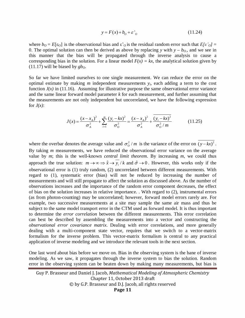
( ) 'O Oy F x b ε= + + (11.24) where bO = E[εO] is the observational bias and ε’O is the residual random error such that E[ε’O] = 0. The optimal solution can then be derived as above by replacing y with y – bO., and we see in this manner that the bias will be propagated through the inverse analysis to cause a corresponding bias in the solution. For a linear model F(x) = kx, the analytical solution given by (11.17) will be biased by gbO. So far we have limited ourselves to one single measurement. We can reduce the error on the optimal estimate by making m independent measurements yi, each adding a term to the cost function J(x) in (11.16). Assuming for illustrative purpose the same observational error variance and the same linear forward model parameter k for each measurement, and further assuming that the measurements are not only independent but uncorrelated, we have the following expression for J(x):
2 22 2
2 2 2 21
( ) ( )( ) ( )( )/
mi iA A
iA O A O
y kx y kxx x x xJ xmσ σ σ σ=
− −− −= + = +∑ (11.25)
where the overbar denotes the average value and 2 /O mσ is the variance of the error on 2( )y kx− . By taking m measurements, we have reduced the observational error variance on the average value by m; this is the well-known central limit theorem. By increasing m, we could thus approach the true solution: ˆ ˆ/ and 0im x y k σ→ ∞ ⇒ → → . However, this works only if the observational error is (1) truly random, (2) uncorrelated between different measurements. With regard to (1), systematic error (bias) will not be reduced by increasing the number of measurements and will still propagate to affect the solution as discussed above. As the number of observations increases and the importance of the random error component decreases, the effect of bias on the solution increases in relative importance. . With regard to (2), instrumental errors (as from photon-counting) may be uncorrelated; however, forward model errors rarely are. For example, two successive measurements at a site may sample the same air mass and thus be subject to the same model transport error in the CTM used as forward model. It is thus important to determine the error correlation between the different measurements. This error correlation can best be described by assembling the measurements into a vector and constructing the observational error covariance matrix. Dealing with error correlations, and more generally dealing with a multi-component state vector, requires that we switch to a vector-matrix formalism for the inverse problem. This vector-matrix formalism is central to any practical application of inverse modeling and we introduce the relevant tools in the next section. One last word about bias before we move on. Bias in the observing system is the bane of inverse modeling. As we saw, it propagates through the inverse system to bias the solution. Random error in the observing system can be beaten down by making many measurements, but bias is

Guy P. Brasseur and Daniel J. Jacob, Mathematical Modeling of Atmospheric Chemistry Chapter 11, October 2013 draft
© by G.P. Brasseur and D.J. Jacob, all rights reserved Page 12
irreducible. If we have some knowledge about the structure of the bias, then we might try to retrieve information on this structure as a component of the state vector. But the central problem of the bias propagating to the solution remains. Minimizing bias in the observing system through independent calibration is thus crucial for inverse modeling. Bias in the instrument can be determined by analysis of known standards, and bias in the forward model can be determined by applying the model to conditions where the state vector is known. Any problematic bias should be corrected before inverse modeling is attempted. If bias in the observing system cannot be characterized, then the error in the inverse model solution cannot be characterized either. In the rest of this chapter and unless otherwise noted we will assume that observational errors are random.
11.4 Vector-Matrix Tools
Let us now consider the problem of a state vector x of dimension n with a priori value xA and associated error εA, for which we seek an optimal estimate x on the basis of an ensemble of observations assembled into an observation vector y of dimension m. y is related to x by the forward model F:
( )= + Oy F x ε (11.26)
where εO is the observational error vector as in (11.1). We have omitted the model parameters p in the expression for F to simplify notation. Inverse analysis requires definition of error statistics and pdfs for vectors. The error statistics are expressed as error covariance matrices, and the pdfs are constructed in a manner that accounts for covariance between vector elements. The forward model must be linearized for application of matrix algebra and this may involve construction of its Jacobian matrix and its adjoint. We describe here these different objects. Their application to solving the inverse problem will be presented in the following sections.
11.4.1 Error Covariance Matrices
The error covariance matrix for a vector is the analog of the error variance for a scalar. Consider a n-dimensional vector x = (x1,…xn)T that we estimate with error ε = (ε1, …εn)
T. The error covariance matrix S for our estimate of x has as diagonal elements (sii) the error variances for the individual components of x, and as off-diagonal elements (sij) the error covariances between components of x:
Guy P. Brasseur and Daniel J. Jacob, Mathematical Modeling of Atmospheric Chemistry Chapter 11, October 2013 draft
© by G.P. Brasseur and D.J. Jacob, all rights reserved Page 13
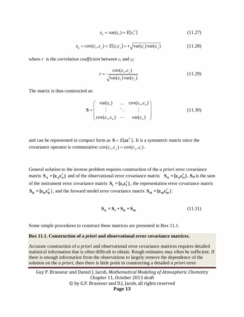
2var( ) [ ]ii i is Eε ε= = (11.27)
cov( , ) [ ] var( ) var( )ij i j i j i js E rε ε ε ε ε ε= = = (11.28) where r is the correlation coefficient between εi and εj:
cov( , )
var( ) var( )i j
i j
rε ε
ε ε= (11.29)
The matrix is thus constructed as:
1 1
1
var( ) cov( , )
cov( , ) var( )
n
n n
ε ε ε
ε ε ε
=
S
(11.30)
and can be represented in compact form as [ ]TE=S εε . It is a symmetric matrix since the covariance operator is commutative: cov( , ) cov( , )i j j iε ε ε ε= .
General solution to the inverse problem requires construction of the a priori error covariance matrix T
A A AS = [ε ε ] and of the observational error covariance matrix TO O OS = [ε ε ] . SO is the sum
of the instrument error covariance matrix TI I IS = [ε ε ] , the representation error covariance matrix
]TR R RS = [ε ε , and the forward model error covariance matrix ]T
M M MS = [ε ε :
O I R MS = S + S + S (11.31)
Some simple procedures to construct these matrices are presented in Box 11.1.
Box 11.1. Construction of a priori and observational error covariance matrices.
Accurate construction of a priori and observational error covariance matrices requires detailed statistical information that is often difficult to obtain. Rough estimates may often be sufficient. If there is enough information from the observations to largely remove the dependence of the solution on the a priori, then there is little point in constructing a detailed a priori error

Guy P. Brasseur and Daniel J. Jacob, Mathematical Modeling of Atmospheric Chemistry Chapter 11, October 2013 draft
© by G.P. Brasseur and D.J. Jacob, all rights reserved Page 14
covariance matrix. For example, one might assume a uniform 50% error on the individual components of xA with no error correlation between the components, in which case SA is a diagonal matrix with elements 0.25xa,i
2. Error correlation between adjacent components of xA can often be represented simply by an e-folding length scale, populating the off-diagonals of SA adjacent to the diagonal. The sensitivity of the inversion to the specification of SA can be tested by repeating the inversion with modified SA and this is good general practice.
The observational error covariance matrix SO can be constructed by adding contributions from the instrument error (SI), representation error (SR), and forward model error (SM). SI is typically a diagonal matrix that can be obtained from knowledge of the instrument precision. SR can be constructed from knowledge of the subgrid variability of observations and can also in general be assumed diagonal. Construction of SM is more difficult as calibration data are generally not available.
An effective shortcut for constructing SO is the residual error method (Heald et al., 2004). In this method, we first apply the forward model to the a priori state vector, compare to observations, and subtract a mean bias to obtain the observational error:
O A Aε = y - F(x ) - y - F(x ) where the averaging can be done over the ensemble of observations or just a subset (for example, the observation time series at a given location). Here we assume that the systematic component of the error in y - F(xA) is due to error in the state vector x to be corrected through the inversion, while the random component is the observational error. The statistics of εO are then used to construct SO. An example is shown in Figure 11.3. The assumption that the systematic error is due solely to x may not be correct, as there may also be bias in the observing system; however, it is consistent with the premise of the inverse analysis that errors be random. From independent knowledge of SI and SR one can infer the forward model error covariance matrix as SM = SO – SI – SR, and from there diagnose the dominant terms contributing to the observational error.

Guy P. Brasseur and Daniel J. Jacob, Mathematical Modeling of Atmospheric Chemistry Chapter 11, October 2013 draft
© by G.P. Brasseur and D.J. Jacob, all rights reserved Page 15
Figure 11.3 Diagonal terms of the observational error covariance matrix constructed for an inversion of CO sources in East Asia in March-April 2001 using MOPITT satellite observations of CO columns. The daily observations are averaged over CTM grid squares and compared to the CTM simulation using a priori sources, producing a time series of CTM-MOPITT differences in each grid square. The mean of that time series is subtracted and the residual difference defines the observational error for that grid square. The resulting error variance is normalized to the mean CO column for the grid square, thus defining a relative error expressed in percentages. The off-diagonal terms of the observational error covariance matrix are derived from an estimated 180-km error correlation length scale. From Heald et al. [2004]. Solution to the inverse problem generates various matrices, as we will see. We may obtain in particular the a posteriori error covariance matrix S for the solution x , in the same way that solution to the inverse problem using scalars yielded an error variance σ for the solution x . This error covariance matrix includes covariances between different solution elements that are often difficult to interpret. Spectral decomposition of the matrix can be useful for identifying error patterns. In the general case, the error covariance matrix S for a vector x has full rank n, since otherwise would imply that an element is perfectly known. It is also symmetric, as we have seen. It therefore has n orthonormal eigenvectors ei with eigenvalues λi. S can then be decomposed along its eigenvectors as follows:
1
nT
iλ
=
= =∑ Ti i iS e e EΛE (11.32)
Guy P. Brasseur and Daniel J. Jacob, Mathematical Modeling of Atmospheric Chemistry Chapter 11, October 2013 draft
© by G.P. Brasseur and D.J. Jacob, all rights reserved Page 16
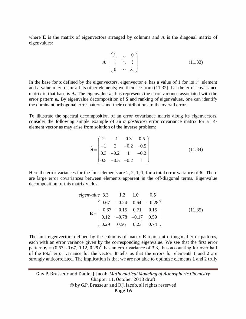
where E is the matrix of eigenvectors arranged by columns and Λ is the diagonal matrix of eigenvalues:
1 0
0 n
λ
λ
=
Λ
(11.33)
In the base for x defined by the eigenvectors, eigenvector ei has a value of 1 for its ith element and a value of zero for all its other elements; we then see from (11.32) that the error covariance matrix in that base is Λ. The eigenvalue λi thus represents the error variance associated with the error pattern ei. By eigenvalue decomposition of S and ranking of eigenvalues, one can identify the dominant orthogonal error patterns and their contributions to the overall error. To illustrate the spectral decomposition of an error covariance matrix along its eigenvectors, consider the following simple example of an a posteriori error covariance matrix for a 4-element vector as may arise from solution of the inverse problem:
2 1 0.3 0.51 2 0.2 0.5ˆ
0.3 0.2 1 0.20.5 0.5 0.2 1
− − − − = − − − −
S (11.34)
Here the error variances for the four elements are 2, 2, 1, 1, for a total error variance of 6. There are large error covariances between elements apparent in the off-diagonal terms. Eigenvalue decomposition of this matrix yields
3.3 1.2 1.0 0.50.67 0.24 0.64 0.280.67 0.15 0.71 0.15
0.12 0.78 0.17 0.590.29 0.56 0.23 0.74
eigenvalue− −
− − = − −
E (11.35)
The four eigenvectors defined by the columns of matrix E represent orthogonal error patterns, each with an error variance given by the corresponding eigenvalue. We see that the first error pattern e1 = (0.67, -0.67, 0.12, 0.29)T has an error variance of 3.3, thus accounting for over half of the total error variance for the vector. It tells us that the errors for elements 1 and 2 are strongly anticorrelated. The implication is that we are not able to optimize elements 1 and 2 truly

Guy P. Brasseur and Daniel J. Jacob, Mathematical Modeling of Atmospheric Chemistry Chapter 11, October 2013 draft
© by G.P. Brasseur and D.J. Jacob, all rights reserved Page 17
independently, and that we could greatly decrease the error in the solution of our inverse problem by merging these two elements of the state vector.
11.4.2 Gaussian Probability Distribution Functions for Vectors
Application of Bayes’ theorem to the vector-matrix formalism requires formulation of probability distribution functions for vectors. We derive here the general Gaussian pdf formulation for a vector x of dimension n with expected value E[x] and error covariance matrix S. If the departures from the expected values for the individual elements of x are uncorrelated (i.e., if S is diagonal), then the pdf of the vector is simply the product of the pdfs for the individual elements. This simple solution can be obtained by projecting x on the basis of eigenvectors ei of S with i = [1,…n]. Let z = ET (x – E[x]) be the value of x – E[x] in the eigenvector basis, where E is the matrix of eigenvectors arranged by columns. The pdf of z is then
2 2
1/2 /2 1/2
1 1( ) exp[ ] exp[ ](2 ) 2 (2 ) 2
i in
ii i i i ii
z zPπλ λ π λ λ
= − = −
∑∏ ∏
z (11.36)
which can be rewritten as
11/2/2
1 1( ) exp[ ]2(2 )
Tn
Pπ
−= −z z Λ zS
(11.37)
Here |S| is the determinant of S, equal to the product of its eigenvalues:
λ= ∏ ii
S (11.38)
and Λ is the diagonal matrix of eigenvalues (11.33). Replacing z in (11.37), we obtain:
1/2/2
1 1( ) exp[ [ ] [ ] ]2(2 )
T Tn
P E Eπ
= − -1x (x - x ) EΛ E (x - x )S
(11.39)
Recall the matrix spectral decomposition S = EΛET (equation (11.32). A matrix and its inverse have the same eigenvectors and inverse eigenvalues so that S-1 = EΛ-1ET. Replacing into (11.39) we obtain the general pdf expression for the vector x:

Guy P. Brasseur and Daniel J. Jacob, Mathematical Modeling of Atmospheric Chemistry Chapter 11, October 2013 draft
© by G.P. Brasseur and D.J. Jacob, all rights reserved Page 18
1/2/2
1 1( ) exp[ [ ] [ ] ]2(2 )
Tn
P E Eπ
= − -1x (x - x ) S (x - x )S
(11.40)
11.4.3 Jacobian Matrix
The Jacobian matrix (here denoted K) is a linearized expression of the forward model that enables application of matrix algebra to the inverse problem. It represents the sensitivity of the observation variables y to the state variables x, assembled in matrix form:
∂= ∇ =
∂xyK Fx
(11.41)
with individual elements /ij i jk y x= ∂ ∂ . If the forward model is linear, then K does not depend on x and fully describes the forward model for the purpose of the inversion. If the forward model is nonlinear, then K needs to be calculated initially for the a priori value xA, representing the initial guess for x, and then re-calculated as needed for updated values of x during iterative convergence to the solution. Depending on the degree of non-linearity, K may not need to be re-calculated at every iteration.
Construction of the Jacobian matrix may be done analytically if the forward model is simple, as in a 0-D chemical model where the evolution of concentrations is determined by reaction rate expressions. If the forward model is complicated, such as a 3-D CTM, then the Jacobian must be constructed numerically. This can be done column by column, if the dimension of the state vector is not too large, by successively perturbing the individual elements xi of the state vector by small increments ∆xi and applying the forward model to obtain the resulting perturbation ∆y. One pass of the forward model provides the vector / /i ix x∆ ∆ ≈ ∂ ∂y y , and n passes of the forward model fully construct the Jacobian matrix. If the observations are sparse and the state vector is large, such as in a receptor-oriented problem where we wish to determine the sensitivity of observations at a given location to a large array of variables, then a more effective way to construct the Jacobian is through the model adjoint as described below. If both the state vector and the observation vector are large, then one can use the model adjoint to bypass the calculation of the Jacobian matrix for inverse modeling applications; this adjoint approach to the inverse problem (often called “4-D Var”) is described in Section 11.6.

Guy P. Brasseur and Daniel J. Jacob, Mathematical Modeling of Atmospheric Chemistry Chapter 11, October 2013 draft
© by G.P. Brasseur and D.J. Jacob, all rights reserved Page 19
11.4.4 Model Adjoint
The adjoint of a model is the transpose of its Jacobian matrix. It turns out to be very useful in inverse modeling applications for atmospheric chemistry where observed concentrations are used to constrain a state vector of emissions or concentrations at previous times. We will discuss this in Section 11.7. It can also be an efficient tool for numerical construction of the Jacobian matrix when dim(y) << dim(x). As we will see, by using the adjoint we can construct the Jacobian matrix row by row, instead of column by column, and the number of model simulations needed for that purpose is dim(y) rather than by dim(x). A standard application of the adjoint is to receptor-oriented problems where we seek for example to determine the sensitivity of the model concentration at a particular point to the ensemble of concentrations or emissions at previous times over the 3-D model domain. In that example, dim(y) = 1 but dim(x) can be very large, and a single pass of the adjoint model can deliver the full vector of sensitivities /y∂ ∂x .
To understand how the adjoint works, consider a CTM discretized over time steps [t0,…ti,… tp]. Let y(p) represent the vector of gridded concentrations of dimension m at time tp,. We wish to determine its sensitivity to some state vector x(0) of dimension n at time t0. The corresponding Jacobian matrix is ( ) (0)p∂ ∂Κ = y / x . By the chain rule,
( ) ( ) ( -1) (1) (0)
(0) ( -1) ( -2) (0) (0)
...p p p
p p
∂ ∂ ∂ ∂ ∂= =
∂ ∂ ∂ ∂ ∂
y y y y yK
x y y y x (11.42)
where the right-hand side is a product of matrices. The model adjoint is the transpose, which we then write as
( ) ( 1) (1) (0) (0) (1) ( 1) ( )
( 1) ( 2) (0) (0) (0) (0) ( 2) ( 1)
... ...T T T T T
p p p pT
p p p p
− −
− − − −
∂ ∂ ∂ ∂ ∂ ∂ ∂ ∂= = ∂ ∂ ∂ ∂ ∂ ∂ ∂ ∂
y y y y y y y yK
y y y x x y y y(11.43)
where we have made use of the property that the transpose of a product of matrices is equal to the product of the transposed matrices in reverse order: (AB)T = BTAT. The adjoint model described by (11.43) offers an alternate way of constructing the Jacobian matrix by applying the model successively to the m individual elements of y(p). Consider the application of KT to a unit vector v = (1,0,…0)T where v1 = 1 and all the other elements are zero. A vector to which the adjoint is applied is called an adjoint forcing. Following (11.43), we begin by applying matrix ( ) ( 1)( / )T
p p−∂ ∂y y to this unit vector:
Guy P. Brasseur and Daniel J. Jacob, Mathematical Modeling of Atmospheric Chemistry Chapter 11, October 2013 draft
© by G.P. Brasseur and D.J. Jacob, all rights reserved Page 20
( ),1 ( 1),1
( ),1 ( 1),2( ) ( ),1
( 1) ( 1)
( ),1 ( 1),
/1/0
0 /
p pT
p pp p
p p
p p m
y yy y y
y y
−
−
− −
−
∂ ∂ ∂ ∂ ∂ ∂ = = ∂ ∂ ∂ ∂
yy y
(11.44)
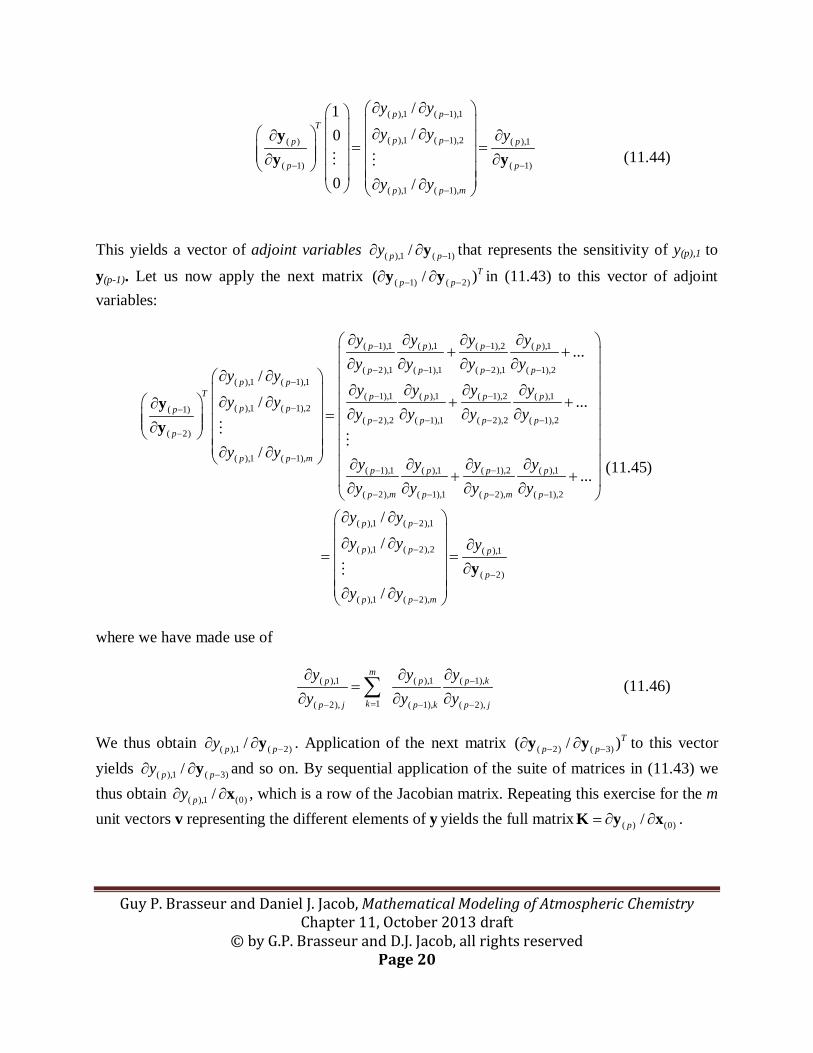
This yields a vector of adjoint variables ( ),1 ( 1)/p py −∂ ∂y that represents the sensitivity of y(p),1 to
y(p-1). Let us now apply the next matrix ( 1) ( 2)( / )Tp p− −∂ ∂y y in (11.43) to this vector of adjoint
variables:
( 1),1 ( ),1 ( 1),2 ( ),1
( 2),1 ( 1),1 ( 2),1 ( 1),2( ),1 ( 1),1
( 1),1 ( ),1( ),1 ( 1),2( 1)
( 2),2 ( 1),1( 2)
( ),1 ( 1),
...//
/
p p p p
p p p pp p
T p pp pp
p pp
p p m
y y y yy y y y
y yy y y
y yy y
y y
− −
− − − −−
−−−
− −−
−
∂ ∂ ∂ ∂+ +
∂ ∂ ∂ ∂∂ ∂
∂ ∂ ∂ +∂ ∂ ∂ ∂ ∂= ∂ ∂ ∂
yy
( 1),2 ( ),1
( 2),2 ( 1),2
( 1),1 ( ),1 ( 1),2 ( ),1
( 2), ( 1),1 ( 2), ( 1),2
( ),1 ( 2),1
( ),
...
...
/
p p
p p
p p p p
p m p p m p
p p
p
yy y
y y y yy y y y
y yy
−
− −
− −
− − − −
−
∂
+ ∂ ∂
∂ ∂ ∂ ∂ + + ∂ ∂ ∂ ∂
∂ ∂
∂=
1 ( 2),2 ( ),1
( 2)
( ),1 ( 2),
/
/
p p
p
p p m
y y
y y
−
−
−
∂ ∂ = ∂ ∂ ∂
y
(11.45)
where we have made use of
( ),1 ( ),1 ( 1),
1( 2), ( 1), ( 2),
mp p p k
kp j p k p j
y y yy y y
−
=− − −
∂ ∂ ∂=
∂ ∂ ∂∑ (11.46)
We thus obtain ( ),1 ( 2)/p py −∂ ∂y . Application of the next matrix ( 2) ( 3)( / )T
p p− −∂ ∂y y to this vector yields ( ),1 ( 3)/p py −∂ ∂y and so on. By sequential application of the suite of matrices in (11.43) we thus obtain ( ),1 (0)/py∂ ∂x , which is a row of the Jacobian matrix. Repeating this exercise for the m unit vectors v representing the different elements of y yields the full matrix ( ) (0)/p= ∂ ∂K y x .
Guy P. Brasseur and Daniel J. Jacob, Mathematical Modeling of Atmospheric Chemistry Chapter 11, October 2013 draft
© by G.P. Brasseur and D.J. Jacob, all rights reserved Page 21
Notice from the above description that a single pass with the adjoint yields the sensitivity vectors ( ),1 ( 1)/p py −∂ ∂y , ( ),1 ( 2)/p py −∂ ∂y , … ( ),1 (0)/py∂ ∂y . This effectively integrates the CTM back in time,
providing the sensitivity of the concentration at a given location and time (here y(p),1) to the complete field of concentrations at prior times, i.e., the backward influence function. The same single pass with the adjoint can also provide the sensitivities of y(p),1 to the state vector at any prior times: thus
( ),1 ( ),1
( ),1 ( ),2( ) ( ),1
( ) ( )
( ),1 ( ),
/1/0
0 /
p pT
p pp p
p p
p p m
y xy x y
y x
∂ ∂ ∂ ∂∂ ∂ = = ∂ ∂ ∂ ∂
yx x
(11.47)
( ),1 ( 1),1
( ),1 ( 1),2( 1) ( ) ( ),1
( 1) ( 1) ( 1)
( ),1 ( 1),
/1/0
0 /
p pT T
p pp p p
p p p
p p m
y xy x y
y x
−
−−
− − −
−
∂ ∂ ∂ ∂∂ ∂ ∂ = = ∂ ∂ ∂ ∂ ∂
y yx y x
(11.48)
( ),1 ( 2),1
( ),1 ( 2),2( 2) ( 1) ( ) ( ),1
( 2) ( 2) ( 1) ( 2)
( ),1 ( 2),
/1/0
0 /
p pT T T
p pp p p p
p p p p
p p m
y xy x y
y x
−
−− −
− − − −
−
∂ ∂ ∂ ∂∂ ∂ ∂ ∂ = = ∂ ∂ ∂ ∂ ∂ ∂
y y yx y y x
(11.49)
and so on. For example, if the state vector represents the emission field, we can obtain in this manner the sensitivity of the concentration y(p),1 to the emissions at all prior time steps, representing a backward influence function for emissions. Figure 11.4 shows the application of a CTM adjoint to determine the sensitivity of the surface ozone concentration at a receptor site to the global distribution of ozone production at prior times. Here the state vector is the 3-D production rate PO3 (expressed as odd oxygen) on the CTM grid.

Guy P. Brasseur and Daniel J. Jacob, Mathematical Modeling of Atmospheric Chemistry Chapter 11, October 2013 draft
© by G.P. Brasseur and D.J. Jacob, all rights reserved Page 22
Figure 11.4 Sensitivity of surface ozone at Mt. Batchelor Observatory, Oregon on April 17-May 15, 2006 to the global distribution of ozone production PO3 at prior times, as calculated in a single pass of the adjoint of a global CTM. The adjoint was initialized with an adjoint forcing on May 15 and integrated backward in time until March 1, with additional unit forcings for individual time steps going back to April 17. The figure shows the global distribution of weighted sensitivities 3 3 3( [ ] / )O OO P P∂ ∂ integrated vertically over the tropospheric column and temporally over all previous times. From Zhang et al. [2009]. We may also wish to determine the sensitivity of the concentrations y(p.1) at time tp to a time-invariant state vector x, such as constant emissions. This follows immediately from the above by viewing x as the sum of contributions of emissions for individual time steps:
( )0
p
ii=
= ∑x x (11.50)
and summing the sensitivities determined from the single pass by the adjoint:
( ),1 ( ),1
0 ( )
pp p
i i
y y
=
∂ ∂=
∂ ∂∑x x (11.51)
Here the computed sensitivity will evidently depend on the choice of the integration time window [t0, tp]. Adjoint sensitivities are generally summed in some way (such as in Figure 11.4) to provide the most relevant information. We have illustrated how the adjoint can provide the sensitivity of concentrations to a state vector, but it can more generally provide the sensitivity of any concentration-related metric. For example, Figure 11.5 (from Bowman and Henze, 2012) applies the adjoint of a CTM to describe the sensitivity of the global radiative forcing from tropospheric ozone to the global distribution

Guy P. Brasseur and Daniel J. Jacob, Mathematical Modeling of Atmospheric Chemistry Chapter 11, October 2013 draft
© by G.P. Brasseur and D.J. Jacob, all rights reserved Page 23
of NOx emissions, where NOx is a precursor for ozone formation. Here the state vector x is the global 2-D field of NOx emissions on the CTM grid, and the model adjoint KT in (11.43) is applied to the vector ( ) ( )/p pF∂ ∂y where F(p) is the global top-of-atmosphere radiative flux in the IR absorption band of ozone at time tp and y(p) is the corresponding global distribution of ozone concentrations. Note that ( ) ( )/p pF∂ ∂y must itself be derived from the adjoint of a radiative transfer model.
Figure 11.5 Adjoint calculation of the spatially-dependent contributions of NOx emissions to the global radiative forcing from tropospheric ozone. The adjoint of a global CTM coupled to a radiative transfer model is used to calculate the sensitivities /F∂ ∂ NOxE , where F is the global top-of-atmosphere radiative flux in the ozone IR absorption band and ENOx is a state vector of NOx emissions on the 2ox2.5o CTM grid. The sensitivities are then multiplied by the local NOx emissions Ei and the corresponding field of ( / )i iF E E∂ ∂ is plotted here. From Bowman and Henze (2012).
We now turn to the specific task of constructing the adjoint for a CTM. This requires linearization of the CTM to express it as a product of matrices that we can then transpose. The CTM calculates the evolution of concentrations over at time step [ti, ti+1] by a succession of operators describing the different model processes. Consider a CTM including 3-D advection (operator A), chemistry (operator C), and emissions (operator E), with operator splitting described by
( 1) ( )( )i iA C E+ =y y (11.52)
where the symbol means “applied to”. The operators may or may not be linear in y. If not, they need to be linearized. This can be done by Taylor expansion as described by (11.2), and the resulting linear model is called the Tangent Linear Model (TLM) of the CTM. Construction of

Guy P. Brasseur and Daniel J. Jacob, Mathematical Modeling of Atmospheric Chemistry Chapter 11, October 2013 draft
© by G.P. Brasseur and D.J. Jacob, all rights reserved Page 24
the TLM can be an arduous task of analytical differentiation of the code, and commercial software packages are available for this purpose. Let A, C, E represent the matrices of the linear or linearized operators. We then have:
( 1) ( )i i+ =y ACEy (11.53) so that
( 1)
( )
i
i
+∂=
∂y
ACEy
(11.54)
The transpose is given by
( 1)
( )
T
i T T T
i
+ ∂= ∂
yE C A
y (11.55)
which is the form we seek.
The simple case of linear operators offers insight into the physical meaning of the adjoint. Let us begin with the advection operator. 3-D advection is generally described by operator splitting with 1-D operators. Consider then a 1-D advection algorithm using a linear upstream scheme on an Eulerian grid:
( 1), ( ), 1 ( ),(1 )i j i j i jy cy c y+ −= + − (11.56)
where c is the Courant number and the flow is from gridbox j-1 to j. Let us assume for the sake of a simple illustrative example that a uniform cyclical flow applies over a domain j = [1, 3]. Then the advection operator is written in matrix form as
( 1)
( )
1 01 0
0 1
i
i advection
c cc c
c c
+
− ∂ = = − ∂ −
yA
y (11.57)
and its transpose is

Guy P. Brasseur and Daniel J. Jacob, Mathematical Modeling of Atmospheric Chemistry Chapter 11, October 2013 draft
© by G.P. Brasseur and D.J. Jacob, all rights reserved Page 25
( 1)
( )
1 00 1
0 1
T
iT
i advection
c cc c
c c
+
− ∂ = = − ∂ −
yA
y (11.58)
We see that the transpose describes the reverse of the actual flow:
( 1), ( ), 1 ( ),(1 )i j i j i jy cy c y+ += + − (11.59) This result is readily generalizable to any number of gridboxes and non-uniform flow. Thus the adjoint of a linear transport operator is simply the reverse flow. Transport operators used in research models are generally not exactly linear because of safeguards for stability or mass conservation. Nevertheless, the approximation of reverse flow is frequently used as an approximation to construct the adjoint because of its simplicity. Consider now a first-order loss chemistry operator dy/dt = -ky where k is a loss rate constant. Application of this operator over a time step ∆t is expressed in matrix form as follows:
( 1)
( )
exp[ ] 0 00 exp[ ] 00 0 exp[ ]
i
i chemistry
k tk t
k t
+
− ∆ ∂ = = − ∆ ∂ − ∆
yC
y (11.60)
which is a diagonal matrix. In this case the transpose operator is the same as the original operator; we refer to the operator as self-adjoint. It makes sense that the sensitivity going back in time should decay with the same time constant as the first-order chemical loss. Finally, let us consider the emission operator E . It does not involve sensitivity to the concentration field for the prior time step, so that it is described by the identity matrix Im and is also self-adjoint:
( 1)
( )
i
i emissions
+ ∂= = ∂
m
yE I
y (11.61)
In this manner the adjoint model marches back in time to describe the sensitivity of concentrations at time tn to concentrations at prior times by successive application of the transposes of the advection, chemistry, and emission operators. At individual time steps we may wish to calculate the sensitivity to the state vector, such as (0) (0)/∂ ∂y x in equation (11.43), and this operator requires its own adjoint. If the state vector represents emissions then the operator is self-adjoint since concentrations will respond only to emission in their own gridbox.
Guy P. Brasseur and Daniel J. Jacob, Mathematical Modeling of Atmospheric Chemistry Chapter 11, October 2013 draft
© by G.P. Brasseur and D.J. Jacob, all rights reserved Page 26
Another simple application of the adjoint is to linear multi-box models, often used in biogeochemical modeling to simulate the evolution of concentrations in m different coupled reservoirs (boxes). The model is described by
ddt
=y Ky + s (11.62)
where y is the vector of concentrations or masses in the different boxes, K is a Jacobian matrix of transfer coefficients kij describing the transfer between boxes, and s is a source vector. Starting from initial conditions at time t0, the evolution of the system for one time step Δt = t1 – t0 is given in forward finite difference form by
(1) (0) (0) t= + ∆y My s (11.63) where t= ∆mM I + K . We see that (1) (0)/∂ ∂ =y y M and (1) (0)/ t∂ ∂ = ∆my s I ; the corresponding adjoint operators are MT and ImΔt (the source operator is self-adjoint). Consider a time period of interest [t0, tp] (say from pre-industrial to present time). A single pass of the adjoint following the procedures given above yields the sensitivity of the concentrations in a given box at a given time to the concentrations and sources in previous times and for all other boxes.
11.5 Analytical Inversion
The vector-matrix tools presented in section 11.4 allow us to apply Bayes’s theorem (Section 11.2) to obtain an optimal estimate of a state vector x (dim n) on the basis of the observation vector y (dim m), the a priori information xA, the forward model F and its Jacobian K = ∇xF , and the error covariance matrices SA and SΟ. The reader is encouraged to return to section 11.3 as needed for the simple application to the scalar inversion problem, which helps develop intuition for the material presented here. Many of the equations derived here have scalar equivalents in section 11.3. The presentation in this section draws heavily from Rodgers (2000).
11.5.1 Optimal Estimate
Folllowing the general Gaussian pdf formulation for vectors (Section 11.4.2), the pdfs to be used for application of Bayes’ theorem are given by
-1
12 ln ( ) ( ) ( )TP c− = − − +A A Ax x x S x x (11.64)
122 ln ( ) ( ( )) ( )TP c−− = − − +Oy | x y F x S y F(x) (11.65)

Guy P. Brasseur and Daniel J. Jacob, Mathematical Modeling of Atmospheric Chemistry Chapter 11, October 2013 draft
© by G.P. Brasseur and D.J. Jacob, all rights reserved Page 27
from which we obtain by Bayes’ theorem:
-1 132 ln ( ) ( ) ( ) ( ) ( )T TP c−− = − − + − − +A A A Ox | y x x S x x y F(x) S y F(x) (11.66)
Here c1, c2, c3 are constants. The optimal estimate or maximum a posteriori (MAP) solution is defined by the maximum of P(x|y), or equivalently the minimum of the scalar-valued χ2 cost function J(x):
-1( ) ( ) ( ) ( ) ( )T TJ = − − + − −-1a A a Ox x x S x x y F(x) S y F(x) (11.67)
To find this minimum, we solve for ( ) :J∇ =x x 0
1( ) 2 ( ) 2 ( ( ) )TJ −∇ = − + =-1x A A Ox S x x K S F x - y 0 (11.68)
where we recognize the model adjoint KT applied to the weighted observational error
1( ( ) )−OS F x - y . Let us assume that F(x) is linear or can be linearized as given by (11.2), i.e., F(x)
= Kx + c4 where c4 is a constant, and for simplicity of notation let c4 = 0 (this can always be enforced by replacing y by y - c4). We then have
1( ) 2 ( ) 2 ( )TJ −∇ = − + =-1x A A Ox S x x K S Kx - y 0 (11.69)
The solution of (11.69) is straightforward and can be expressed in compact form as
ˆ ( )= + −A Ax x G y Kx (11.70)
where G is the gain matrix given by
1(T T −= +A A OG S K KS K S ) (11.71) or equivalently by:
1 1( )T T− − −= + -1 1O A OG K S K S K S (11.72)
G describes the sensitivity of the retrieval to the observations, i.e., ˆ /= ∂ ∂G x y . It can often be analyzed usefully to determine which of the observations contribute most to constrain a given component of the solution.
Guy P. Brasseur and Daniel J. Jacob, Mathematical Modeling of Atmospheric Chemistry Chapter 11, October 2013 draft
© by G.P. Brasseur and D.J. Jacob, all rights reserved Page 28
The a posteriori error covariance matrix S of x can be calculated as in section 11.3 for the scalar problem by rearranging the right-hand side of (11.66) with F(x) = Kx to be of the form
1ˆˆ ˆ( ) ( )T −− −x x S x x . The algebra is straightforward and yields
1ˆ ( )T −= -1 -1O AS K S K + S (11.73)
Note the similarity of our equations for ˆˆ( ), , , and J x x G S to those derived for scalars in section 11.3.
Three simple checks should be made on the quality of the inverse solution. First, by definition of J we should find ˆ( )J m n≈ +x . Second, we should check that J has indeed been reduced:
ˆ( ) ( )J J< Ax x . Third, it is important to test the solution by applying the forward model to the optimal estimate and comparing the field of ˆF(x) - y to that of F(xA) – y; the errors should be reduced relative to the a priori. In addition, the field of ˆF(x) - y should ideally be uniformly distributed as white noise around zero. Large coherent areas of high (positive or negative) values of ˆF(x) - y suggest model bias or at least a poor characterization of errors.
If m >>n, the minimization of the cost function may be heavily driven by observations with little contribution from the a priori terms. This is formally correct but assumes that the observational error is random and that error covariances are well characterized (see discussion in Section 11.3). Often we have little confidence that this is indeed the case. A way to test this is to introduce a regularization factor γ in the cost function:
-1( ) ( ) ( ) ( ) ( )T TJ γ= − − + − −-1
a A a Ox x x S x x y F(x) S y F(x) (11.74)
which amounts to replacing the observational error covariance matrix SO by SO/γ. The solution x can be readily calculated for different values of γ spanning the range of our confidence in error characterization. By plotting the cost function ˆ( )J x vs. γ, we may find that a value of γ other than 1 would lead to an improved cost function, and if so we will need to make a judgment as to whether this is a more appropriate solution.
As a related issue, we pointed out in Section 11.3 the danger of over-interpreting the reduction in error variance that results from the accumulation of a large number of observations. The same concern applies here. The reduction in error from Sa to S assumes that the observational error is random and that error covariances in the observations are fully accounted for. These requirements are often not satisfied, in which case S will underestimate the actual error on x . A more realistic way of assessing the error in x is then to conduct an ensemble of inverse calculations with various perturbations to model parameters and covariance error estimates (such
Guy P. Brasseur and Daniel J. Jacob, Mathematical Modeling of Atmospheric Chemistry Chapter 11, October 2013 draft
© by G.P. Brasseur and D.J. Jacob, all rights reserved Page 29
as through the regularization factor γ) within their expected uncertainties. Model parameters are often a recognized potential source of bias, so that producing an ensemble based on uncertainties in these parameters can be an effective way to address the effect of biases on the inverse solution.
11.5.2 Averaging Kernel Matrix
A useful way to express the ability of an observational system to constrain the true value of the state vector is with the averaging kernel matrix ˆ∂ ∂A = x/ x , representing the sensitivity of the retrieval x to the true state x. From its definition, A is the product of the gain matrix ˆ /= ∂ ∂G x y and the Jacobian matrix /= ∂ ∂K y x :
A = GK (11.75)
Replacing (11.75) and Oy = Kx + ε into (11.70) we obtain an alternate form for x :
ˆ (= + −n A Ox Ax I A)x + Gε (11.76)
or equivalently ˆ ( (= + − −n A Ox x I A) x x) + Gε (11.77)
where In is the identity matrix of dimension n. Note the similarity to (11.19) and (11.20) in the scalar problem. A is a weighting factor for the relative contributions to the optimal estimate from the true state vs. the a priori estimate. Ax represents the contribution of the true state to the solution, (In – A)xA represents the contribution from the a priori, and GεΟ represents the contribution from the random observational error mapped onto state space by the gain matrix G. A perfect observational system would have A = In. We call (In – A)(xA – x) the smoothing error (because it smoothes the solution towards the a priori) and GεΟ the retrieval error. From (11.77) we can also derive an alternate expression for the error covariance matrix S :
ˆ ˆ ˆ[( ) ] (( )( ) ( ) ) [ ]
(
T T T T T
T T
E E E= = − − +
=n A A n O O
n A n O
S x - x)(x - x I A x x )(x - x I - A Gε ε GI - A)S (I - A) + GS G
(11.78)

Guy P. Brasseur and Daniel J. Jacob, Mathematical Modeling of Atmospheric Chemistry Chapter 11, October 2013 draft
© by G.P. Brasseur and D.J. Jacob, all rights reserved Page 30
from which we see that S can be decomposed into the sum of a smoothing error covariance matrix ( T
n A nI - A)S (I - A) and a retrieval error covariance matrix TOGS G . The smoothing error
covariance matrix describes the smoothing of the solution by the a priori information. The retrieval error covariance matrix describes the noise in the observing system.
Algebraic manipulation yields an alternate form of the averaging kernel matrix as
ˆ −= − 1
n AA I SS (11.79) which relates the improved knowledge of the state vector measured by A to the variance reduction previously discussed for the scalar problem (equation (11.22)).
The averaging kernel matrix constructed from knowledge of SA, SO, and K is a very useful thing to know about an observing system. When designing a system it can be used to evaluate and compare the merits of different designs. By relating the observed state to the true state, it enables comparison of data from different observing systems (Rodgers and Connor, 2003; Zhang et al., 2010) As we will see below, the averaging kernel matrix also quantifies the number of pieces of information provided by an observing system. In the analytical solution to the inverse problem, as described above, the averaging kernel matrix is obtained as part of the solution. However, analytical solution may not be practical when dim(x) is large because of the cost of computing K and of multiplying an inverting large matrices. Numerical solutions to the inverse problem such as from the adjoint method discussed below or from neural networks (Hadji-Lazaro et al., 1999) do not have a computational limit on dim(x) but do not provide averaging kernel matrices as part of their solutions; this is a major shortcoming of these methods for error characterization.
11.5.3 Pieces of Information in an Observing System
A concept related to the average kernel matrix is the number of pieces of information in an observing system towards constraining an n-dimensional state vector. The number of pieces of information is often called the number of degrees of freedom for signal (DOFS). Before making the observations we have n unknowns in the system, representing the n elements of the state vector constrained by the a priori error covariance matrix. We can express that number of unknowns as
[( ) ( )]TE n− − =-1A A ax x S x x (11.80)

Guy P. Brasseur and Daniel J. Jacob, Mathematical Modeling of Atmospheric Chemistry Chapter 11, October 2013 draft
© by G.P. Brasseur and D.J. Jacob, all rights reserved Page 31
After making the observations the error on x is decreased, and we can express this decrease by a reduction in the number of unknowns to ˆ ˆ[( ) ( )]TE − −-1
Ax x S x x . The number of pieces of information from the observations is defined by the decrease in the number of unknowns:
ˆ ˆ ˆ ˆDOFS [( ) ( )] [( ) ( )] [( ) ( )]T T TE E n E= − − − − − = − − −-1 -1 -1A A a A Ax x S x x x x S x x x x S x x (11.81)
The quantity ˆ ˆ( ) ( )T− −-1
Ax x S x x is a scalar and is thus equal to its trace in matrix notation:
ˆ ˆ ˆ ˆ ˆ ˆ( ) ) tr(( ) ( )) tr(( )( ) )T T T− − = − − = − −-1 -1 -1A A Ax x S (x x x x S x x x x x x S (11.82)
Thus
ˆˆ ˆ ˆ ˆ[( ) ( )] [tr(( )( ) )] tr( )T TE E− − = − − =-1 -1 -1A A Ax x S x x x x x x S SS (11.83)
so that
ˆ ˆDOFS tr( ) tr( ) tr( )n= − = − =-1 -1A n ASS I SS A (11.84)
The number of pieces of information in an observing system is thus given by the trace of its averaging kernel matrix. Box 11.2. Example application of analytical inversion.
We illustrate the analytical solution to the inverse problem with the retrieval of carbon monoxide (CO) vertical profiles from the MOPITT satellite instrument (Deeter et al., 2003). The instrument makes nadir measurements of the temperature-dependent IR terrestrial emission at and around the 4.6 µm CO absorption band. Atmospheric CO is detected by its temperature contrast with the surface. The radiances measured at different wavelengths represent the observation vector for the inverse problem. The state vector is chosen to include CO mixing ratios at 7 different vertical levels from the surface to 150 hPa, plus surface temperature and surface emissivity. The forward model is a radiative transfer model (RTM) computing the radiances as a function of the state vector values. The observational error covariance matrix is constructed from knowledge of instrument noise and from comparison of the RTM to a highly accurate (but computationally prohibitive) line-by-line model. The a priori CO vertical profile and its error covariance matrix are derived from a worldwide compilation of aircraft measurements. The a priori surface temperature is specified from local assimilated meteorological data and the a priori surface emissivity is taken from a geographical database. The forward model is non-linear, in particular because the sensitivity to the CO vertical profile depends greatly on the surface temperature; thus a local Jacobian matrix needs to be computed for each scene.

Guy P. Brasseur and Daniel J. Jacob, Mathematical Modeling of Atmospheric Chemistry Chapter 11, October 2013 draft
© by G.P. Brasseur and D.J. Jacob, all rights reserved Page 32
Figure 11.6 (left panel) shows the averaging kernel matrix A constructed in this manner for a typical ocean scene. Here A is plotted row by row for the CO vertical profile elements only, with each line corresponding to a given vertical level indicated in legend. The line for level i gives
ˆ /ix∂ ∂x , the sensitivity of the retrieval at that level to the true CO mixing ratios at different levels. A perfect observing system (A = In) would show unit sensitivity to that level ( ˆ / 1i ix x∂ ∂ = ) and zero sensitivity to other levels. However, we see from Figure 11.6 that the averaging kernel elements are much less than 1 and that the information is smeared across vertical levels. This reflects the observation error in the system.
Figure 11.6. Retrieval of CO mixing ratios by the MOPITT satellite instrument for a scene over the North Pacific in April 2001. Lines with different symbols in the the left panel show the rows of the averaging kernel matrix for 7 vertical levels from the surface to 150 hPa. The right panel shows the MOPITT retrieval (solid line with symbols and a posteriori error variances) together with a vertical profile measured coincidently from aircraft. The dashed line represents the smoothing of the aircraft profile by the MOPITT averaging kernel matrix. From Jacob et al. (2003).
Consider the retrieval of the CO mixing ratio at 700 hPa (blue line). We see that the retrieved value is actually sensitive to CO at all altitudes, i.e., it is not possible from the retrieval to narrowly identify the CO mixing ratio at 700 hPa (or at any other specific altitude). The temperature contrast between vertical levels is not sufficient. We retrieve instead a broad CO column weighted toward the middle troposphere (700-500 hPa). In fact, the retrieval at 700 hPa is more sensitive to the CO mixing ratio at 500 hPa than at 700 hPa. Physically, this means that a given mixing ratio of CO at 500 hPa will give a spectral response similar to a larger mixing ratio at 700 hPa, because 500 hPa has greater temperature contrast with the surface.

Guy P. Brasseur and Daniel J. Jacob, Mathematical Modeling of Atmospheric Chemistry Chapter 11, October 2013 draft
© by G.P. Brasseur and D.J. Jacob, all rights reserved Page 33
Consider now the retrieval of CO in surface air (black line). There is some thermal contrast between surface air and the surface itself, but the signal is very faint. If we had a perfect observing system we could retrieve it; because of observation error, however, the sensitivity of the surface air retrieval to surface air concentrations is close to zero. In fact, the surface air retrieval is very similar to that at 700 hPa and exhibits the same maximum sensitivity at 700-500 hPa.
Inspection of the averaging kernel matrix in Figure 11.6 suggests that the retrieval only provides two independent pieces of information on the vertical profile, one for 700-500 hPa (from the retrievals up to 500 hPa) and one for above 300 hPa (from the retrievals above 350 hPa). We can quantify the DOFS by the trace of the averaging kernel matrix, adding up the ˆ /i ix x∂ ∂ values for the seven vertical levels. We find a DOFS of 1.2. Thus the retrieval mainly provides a CO column weighted toward the middle troposphere, with a smaller independent piece of information in the upper troposphere.
The right panel of Figure 11.6 shows the vertical profile of CO retrieved by MOPITT and compares it to a coincident detailed vertical profile of CO measured from aircraft. The aircraft observations have high accuracy and can be regarded as defining the true vertical profile x. They show a layer of elevated CO at 900-800 hPa that MOPITT does not detect, as would be expected from the discussion above. To determine if the MOPITT retrieval is consistent with the vertical profile measured from aircraft, we need to smooth the aircraft observations with the averaging kernel matrix in order to simulate what MOPITT should actually observe. Smoothing defines a vertical profile x’, shown as the dashed line in the right panel of Figure 11.6:
' n Ax = Ax + (I - A)x (11.85)
This is the expected profile (εO = 0) that MOPITT should see if its capability is as advertised by the error analysis that led to the averaging kernel matrix. We see that the vertical structure from the actual aircraft profile is largely lost, as would be expected (the vertical gradient is mainly from the a priori). But the effective column concentration agrees closely with the MOPITT observation. Such aircraft validation of satellite instruments is critical for identifying retrieval biases or inadequate characterization of retrieval errors.
11.5.4 Sequential Updating
The computational cost of the analytical solution to the inverse problem grows rapidly with the dimensions n and m of the state and observation vectors because of the size of the corresponding matrices that need to be constructed, inverted, and multiplied. The limitation on the size of n can

Guy P. Brasseur and Daniel J. Jacob, Mathematical Modeling of Atmospheric Chemistry Chapter 11, October 2013 draft
© by G.P. Brasseur and D.J. Jacob, all rights reserved Page 34
be addressed by an adjoint solution to the inverse problem, described in section 11.6. The limitation on the size of m can be addressed more simply within the framework of the analytical solution by sequential updating. In this approach, the observation vector is partitioned into smaller “packets” of observations that are successively ingested into the inverse analysis. The solution ( ˆˆ , x S ) obtained after processing of one packet is used as a priori for the next packet, and so on. The final solution is exactly the same as if the entire observation vector were ingested at once. The only limitation is that there be no observational error correlation between packets, i.e., SΟ for the ensemble of observations must be a block diagonal matrix where the blocks are the individual packets. In the simplest case where individual observations are uncorrelated, they can be ingested one by one.
11.6 Adjoint-Based Inversion
The analytical solution to the inverse problem requires construction and manipulation of the Jacobian matrix /= ∂ ∂K y x . Numerical construction of K requires a number n+1 of forward model calculations. If the forward model is non-linear, then K needs to be reconstructed for successive iterations towards the solution. The associated computational costs can be prohibitive and limit the manageable size of the state vector. This is a problem when we have a very large number of observations and would like to constrain a commensurately large state vector. Sequential updating as described in section 11.5.4 can accommodate a very large number of observations but cannot be effectively applied to accommodate a large state vector, if only because the Jacobian still needs to be constructed.
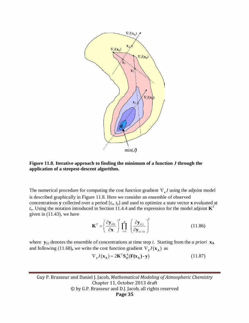
Limitations on the size of the state vector for the inversion can be lifted by using the adjoint of the forward model (Section 11.4.4) to find the minimum of the cost function J(x) in (11.67) numerically rather than analytically. The procedure is illustrated in Figure 11.7. We use the adjoint to calculate the gradient J∇x of the cost function, and a steepest-descent algorithm to converge iteratively to the solution. Starting from an a priori estimate xA for the state vector, we calculate J∇x (xA) and pass it to the steepest-descent algorithm that returns a next guess x1. We then calculate J∇x (x1), pass it to the steepest-descent algorithm that returns a next guess x2, and so on. Convergence is achieved when J(x) does not change significantly anymore from one iteration to the next.
Guy P. Brasseur and Daniel J. Jacob, Mathematical Modeling of Atmospheric Chemistry Chapter 11, October 2013 draft
© by G.P. Brasseur and D.J. Jacob, all rights reserved Page 35
Figure 11.8. Iterative approach to finding the minimum of a function J through the application of a steepest-descent algorithm.
The numerical procedure for computing the cost function gradient J∇x using the adjoint model is described graphically in Figure 11.8. Here we consider an ensemble of observed concentrations y collected over a period [to, tp] and used to optimize a state vector x evaluated at to. Using the notation introduced in Section 11.4.4 and the expression for the model adjoint KT
given in (11.43), we have
(0) ( )
1 ( 1)
TT piT
i i= −
∂ ∂ = ∂ ∂
∏y y
Kx y
(11.86)
where y(i) denotes the ensemble of concentrations at time step i. Starting from the a priori xA and following (11.68), we write the cost function gradient ( )J∇x Ax as
( ) 2 ( )TJ∇ = -1x A O Ax K S F(x ) - y (11.87)

Guy P. Brasseur and Daniel J. Jacob, Mathematical Modeling of Atmospheric Chemistry Chapter 11, October 2013 draft
© by G.P. Brasseur and D.J. Jacob, all rights reserved Page 36
Figure 11.8. Graphical representation of the adjoint method for numerical computation of the cost function gradient ( ) 2 ( )TJ∇ = -1
x A O Ax K S F(x ) - y evaluated at xA (equation (11.87)). We assune here an ensemble of observed concentrations over the period [to, tp] used to optimize the state vector x evaluated at time to. We start with a pass of the forward model F(xA) over the observation period [to, tp]. From there we collect adjoint forcings
)−-1O AS (F(x ) y (in red) for the ensemble of observations. We force the adjoint model with
the adjoint forcings at time tp and propagate these forcings back in time with the adjoint model (in blue), adding new forcings as we march backward in time from tp to to and pick up new observations along the way. At time to we apply the final operation ( )(0) /
T∂ ∂y x to
the adjoint variables to obtain the cost function gradient ( )J∇x Ax . See text for more details.
where the model adjoint is applied to the vector )−-1O AS (F(x ) y representing the error-weighted
differences between the forward model and the observations. The components of )−-1O AS (F(x ) y

Guy P. Brasseur and Daniel J. Jacob, Mathematical Modeling of Atmospheric Chemistry Chapter 11, October 2013 draft
© by G.P. Brasseur and D.J. Jacob, all rights reserved Page 37
are called the adjoint forcings. We make one pass of the forward model F(xA) through the observational period [to, tp] and collect the corresponding adjoint forcing terms )−-1
O AS (F(x ) y , which may be scattered over the period. Starting from the observations y(p) at tp , we apply the first adjoint operator ( )( ) ( 1)/
T
p p−∂ ∂y y from equation (11.86) to the adjoint forcing terms
( ) )p−-1O AS (F(x ) y to obtain the adjoint variables ( )( ) ( 1) ( )/ )
T
p p p−∂ ∂ −-1O Ay y S (F(x ) y as a 3-D field
on the model grid. We then add to these adjoint variables the adjoint forcings ( 1) )p−−-1
O AS (F(x ) y from the observations at time tp-1, apply the next adjoint operator
( )( 1) ( 2)/T
p p− −∂ ∂y y to the resulting quantities, and so on until time to when the final application of
the adjoint operator ( )(0) /T
∂ ∂y x returns the quantity ( )T -1O AK S F(x ) - y = ( )J∇x Ax from (11.87).
The procedure can be readily generalized to obtain the cost function gradient for a time-invariant state vector, or for observations other than concentrations; see related discussion in Section 11.4.4. Once ( )J∇x Ax is calculated we pass it to the steepest-descent algorithm to make an updated guess x1 for the state vector. We then recalculate ( )J∇x 1x for that updated guess,
( ) 2 ( ) 2 ( )TJ∇ = − +-1 -1x 1 A 1 A O 1x S x x K S F(x ) - y (11.88)
using the same adjoint method as before to obtain ( )T -1O 1K S F(x ) - y and adding the terms
( )−-1A 1 AS x x which are now non-zero. We pass ( )J∇x 1x to the steepest-descent algorithm
which makes an updated guess x2 and so on until convergence. A critical feature of the adjoint method is that the Jacobian matrix K is never constructed. We do not in fact need the sensitivity of individual observations to x, which is what K would give us. All we need is the summed sensitivity ( )T -1
O AK S F(x ) - y , which is what the adjoint method provides. Increasing the number of observations does not induce additional computing costs, as it just amounts to updating the adjoint variables on the forward model grid to add new adjoint forcings (Figure 11.7). Increasing the number of state variables (that is, the size of x) incurs little computing cost either, although it may require more iterations to achieve convergence by the steepest-descent algorithm. Construction of the adjoint model may involve approximations in the linearization of the forward model. The accuracy of the cost function gradients ( )J∇x x produced by the adjoint method can be checked with a simple finite-difference test. The test involves applying the forward model to xA , calculating the cost function J(xA), and repeating for a small perturbation to one of the
Guy P. Brasseur and Daniel J. Jacob, Mathematical Modeling of Atmospheric Chemistry Chapter 11, October 2013 draft
© by G.P. Brasseur and D.J. Jacob, all rights reserved Page 38
elements xA + ∆xA where ∆xA has value ∆xi for element i and zero for all other elements. The resulting finite-difference approximation
( ) ( )( )i
J JJx
+ ∆ −∇ ≈
∆A A A
x Ax x xx (11.89)
can then be compared to the value obtained with the adjoint model. It is tempting in adjoint-based inversions to choose a very large state vector to optimize, since computational cost does not depend on state vector size. However, choosing too large a state vector relative to the amount of information provided by the observations results in an inability of the observations to properly constrain the state vector. This is because the observations have then little sensitivity to individual elements of the state vector and thus cannot pull them away from the a priori. Consider the general form of the cost function gradient in (11.68). As dim(x) increases, the Jacobian matrix values become smaller and thus the individual terms of
1( ( ) )T −OK S F x - y decrease in magnitude as TK distributes 1( ( ) )−
OS F x - y over a larger number of state vector elements. By contrast, the magnitude of individual terms of -1( )−A AS x x does not change. Thus the a priori increases in importance relative to the observations. The problem can be mitigated by accurately specifying a priori error correlations or by imposing correlations in the solution, as is done in geostatistical inversions (see below). But we may not have adequate information to impose those constraints. An alternative is to seek empirically the optimal dimension of the state vector as that which provides the best fit to observations. We can measure this fit by ˆ ˆ( ) ( )T− −-1
Oy F(x) S y F(x) where x is the inverse solution and SO is the observational error covariance matrix for the highest-resolution inversion. Too large a state vector x will hinder the fit to observations, as described above. However, too small a state vector will also hinder the fit by failing to optimize variables that could be optimized. Consider for example two state vector elements (x1, x2) that we aggregate into a single element x1
’. In that case the inversion will only optimize x1
’ and conserve the ratio x2/x1 even though that ratio may be in error. The resulting error is called the aggregation error and is part of the forward model error, since the ratio x2/x1 is now effectively a model parameter (section 11.1). By conducting a series of inversions with varying numbers of state vector elements, starting from the largest practical number and gradually aggregating elements with a hierarchical clustering algorithm, one can find the optimal number of state vector elements that will provide the best fit to observations by balancing the strength of the observational constraints against the aggregation error (Figure 11.9).

Guy P. Brasseur and Daniel J. Jacob, Mathematical Modeling of Atmospheric Chemistry Chapter 11, October 2013 draft
© by G.P. Brasseur and D.J. Jacob, all rights reserved Page 39
Figure 11.9. Optimization of the number of state vector elements in an inversion, measured by the ability of the solution x to match observations. Too few state vector elements lead to excessive aggregation error, while too many state vector elements limit the ability of the solution to depart from the a priori.
11.7 Geostatistical Inversions
In some inverse problems we may have good a priori knowledge of state vector patterns but not of their magnitudes. For example, in an inverse problem optimizing emissions we may know that emissions relate to population density for which we have good a priori information, even if we don’t have good information for the emissions themselves. We refer to an inversion that places a priori constraints on state vector patterns rather than magnitudes as a geostatistical inversion. The optimization differs from the Bayesian approach. Let us consider that we have q normalized pattern vectors (p1,...pq), each of dimension n, to describe the state vector x of dimension n. In the above example each pattern might represent a source type, and the state vector then sums the emissions from all source types. We seek a solution of the form x = Pβ where P is the matrix of pattern vectors arranged column by column and β is a vector of multiplicative coefficients to be applied to each pattern. The simplest solution is obtained by a multilinear regression (MLR) fit where we force the observations y to to match the a priori patterns and obtain the resulting coefficients β. The cost function J(β) is then
( ) ( ) ( )TJ = -1
Oβ y - F(Pβ) S y - F(Pβ) (11.90)
Guy P. Brasseur and Daniel J. Jacob, Mathematical Modeling of Atmospheric Chemistry Chapter 11, October 2013 draft
© by G.P. Brasseur and D.J. Jacob, all rights reserved Page 40
where F is the forward model and SO is the observational error covariance matrix. The minimization involves solving ( )J∇ =β β 0 . This is readily done with standard MLR software packages. The ability of the MLR to fit the data provides a test for the a priori model x = Pβ.
The more general geostatistical inversion approach (Michalak et al., 2004; Miller et al., 2012) allows for departure of the solution from the a priori patterns. Here we optimize for both x and β with the cost function
-1( , ) ( ) ( ) ( ) ( )T TJ = − − + − −-1
Ox β x Pβ S x Pβ y F(x) S y F(x) (11.91)
where Pβ now represents an a priori model for the mean of x, from which the solution for individual elements can depart. The covariance matrix S gives the a priori covariances of x, rather than the error covariances.
11.8 Data assimilation
Data assimilation refers to a particular kind of inverse problem where we seek to optimize a time-dependent 3-D model field of state variables based on observations of these or related variables (Section 11.1). This is of great importance in weather forecasting where one must optimize the initial 3-D state of the meteorological variables driving the forecast. Chemical data assimilation gemerally involves optimization of 3-D gridded fields of concentrations. It can play a role in the weather forecast if the chemicals influence the weather (e.g., aerosols) or provide indirect information on meterological variables (stratospheric ozone). Other applications of chemical data assimilation include air quality forecasts and intercomparisons of instruments viewing different scenes. The model used to generate the chemical forecast for data assimilation will be referred to here as the forecast model. It may be a CTM driven by input meteorological forecasts from a GCM, but it is in general better for the chemical forecast to be done within the GCM to achieve consistency between meteorological and chemical data assimilation.
The state vector x and the observation vector y in data assimilation are both very large, and x evolves with time as determined by the forecast model and the assimilated observations. The model initialized with x(0) at time t0 produces a forecast x(1) for time t1 = t0 +h, where h is typically of the order of a day (much longer than the internal time step of the forecast model). Two different strategies can be used to assimilate the observations (Figure 11.10). In the Kalman filter (also called 3DVAR), observations are assembled at the discrete forecast time steps t0, t0 + h, t0 + 2h, etc. and used to optimize the state vector at the corresponding times, with the information then propagated in time through the forecast model. In variational data assimilation
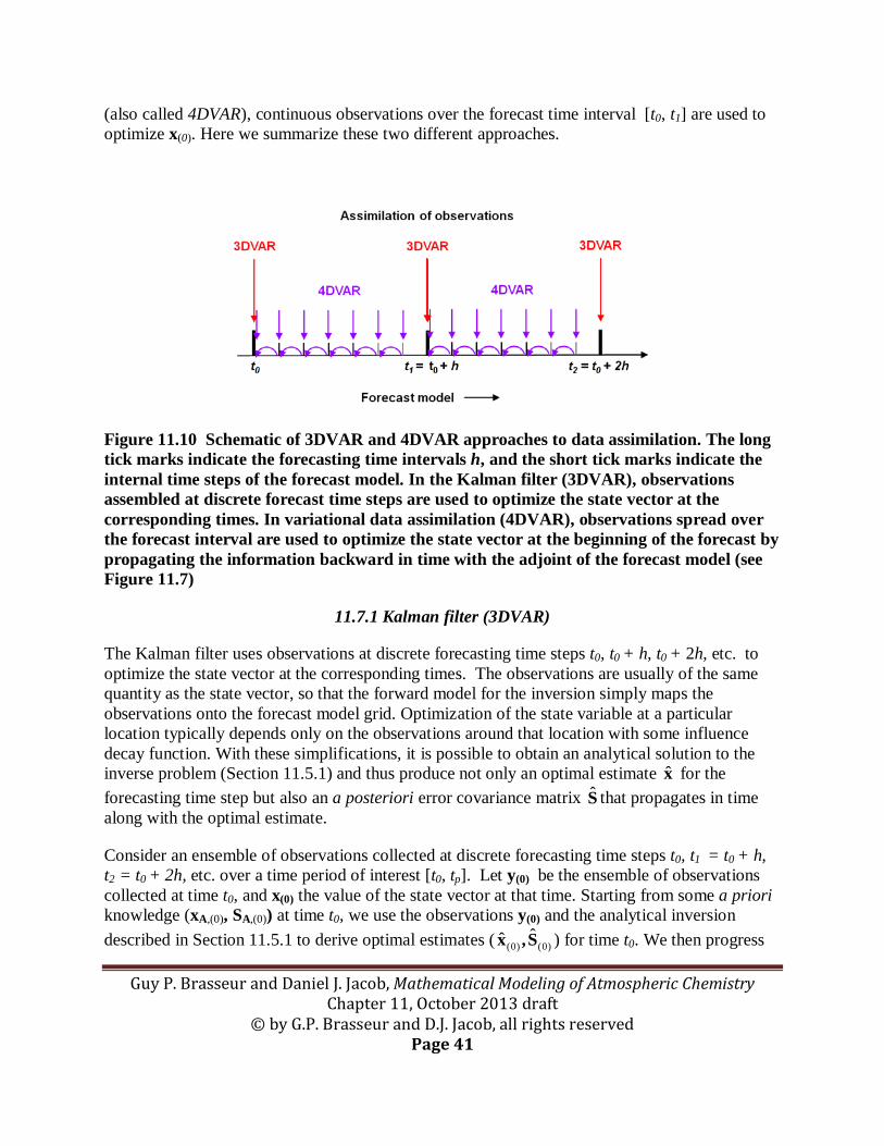
Guy P. Brasseur and Daniel J. Jacob, Mathematical Modeling of Atmospheric Chemistry Chapter 11, October 2013 draft
© by G.P. Brasseur and D.J. Jacob, all rights reserved Page 41
(also called 4DVAR), continuous observations over the forecast time interval [t0, t1] are used to optimize x(0). Here we summarize these two different approaches.
Figure 11.10 Schematic of 3DVAR and 4DVAR approaches to data assimilation. The long tick marks indicate the forecasting time intervals h, and the short tick marks indicate the internal time steps of the forecast model. In the Kalman filter (3DVAR), observations assembled at discrete forecast time steps are used to optimize the state vector at the corresponding times. In variational data assimilation (4DVAR), observations spread over the forecast interval are used to optimize the state vector at the beginning of the forecast by propagating the information backward in time with the adjoint of the forecast model (see Figure 11.7)
11.7.1 Kalman filter (3DVAR)
The Kalman filter uses observations at discrete forecasting time steps t0, t0 + h, t0 + 2h, etc. to optimize the state vector at the corresponding times. The observations are usually of the same quantity as the state vector, so that the forward model for the inversion simply maps the observations onto the forecast model grid. Optimization of the state variable at a particular location typically depends only on the observations around that location with some influence decay function. With these simplifications, it is possible to obtain an analytical solution to the inverse problem (Section 11.5.1) and thus produce not only an optimal estimate x for the forecasting time step but also an a posteriori error covariance matrix S that propagates in time along with the optimal estimate.
Consider an ensemble of observations collected at discrete forecasting time steps t0, t1 = t0 + h, t2 = t0 + 2h, etc. over a time period of interest [t0, tp]. Let y(0) be the ensemble of observations collected at time t0, and x(0) the value of the state vector at that time. Starting from some a priori knowledge (xA,(0), SA,(0)) at time t0, we use the observations y(0) and the analytical inversion described in Section 11.5.1 to derive optimal estimates ( (0) (0)
ˆx ,S ) for time t0. We then progress
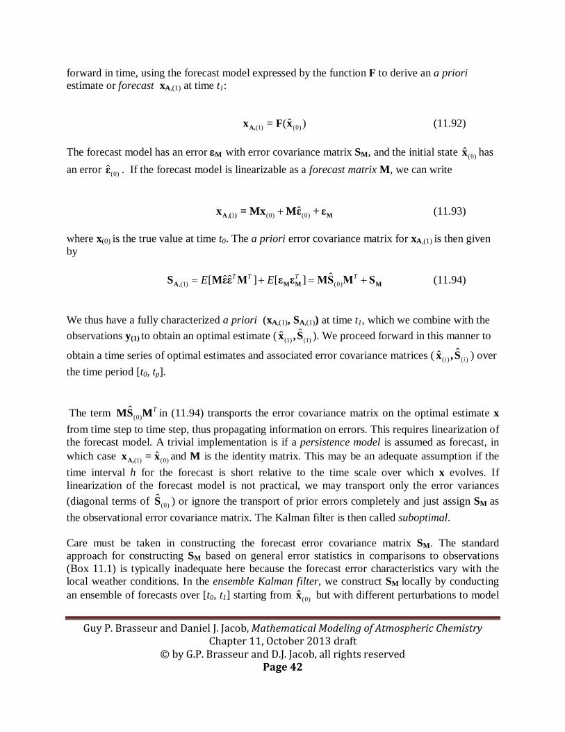
Guy P. Brasseur and Daniel J. Jacob, Mathematical Modeling of Atmospheric Chemistry Chapter 11, October 2013 draft
© by G.P. Brasseur and D.J. Jacob, all rights reserved Page 42
forward in time, using the forecast model expressed by the function F to derive an a priori estimate or forecast xA,(1) at time t1:
(1) (0)ˆ( )A,x = F x (11.92)
The forecast model has an error εM with error covariance matrix SM, and the initial state (0)x has an error (0)ε . If the forecast model is linearizable as a forecast matrix M, we can write
, 1 (0) (0)ˆ+A ( ) Mx = Mx Mε + ε (11.93)
where x(0) is the true value at time t0. The a priori error covariance matrix for xA,(1) is then given by
,(1) (0)ˆˆˆ[ ] [ ]T T T TE E= + = +A M M MS Mεε M ε ε MS M S (11.94)
We thus have a fully characterized a priori (xA,(1), SA,(1)) at time t1, which we combine with the observations y(1) to obtain an optimal estimate ( (1) (1)
ˆx ,S ). We proceed forward in this manner to
obtain a time series of optimal estimates and associated error covariance matrices ( ( ) ( )ˆˆ i ix ,S ) over
the time period [t0, tp]. The term (0)
ˆ TMS M in (11.94) transports the error covariance matrix on the optimal estimate x from time step to time step, thus propagating information on errors. This requires linearization of the forecast model. A trivial implementation is if a persistence model is assumed as forecast, in which case (1) (0)ˆA,x = x and M is the identity matrix. This may be an adequate assumption if the time interval h for the forecast is short relative to the time scale over which x evolves. If linearization of the forecast model is not practical, we may transport only the error variances (diagonal terms of (0)S ) or ignore the transport of prior errors completely and just assign SM as the observational error covariance matrix. The Kalman filter is then called suboptimal. Care must be taken in constructing the forecast error covariance matrix SM. The standard approach for constructing SM based on general error statistics in comparisons to observations (Box 11.1) is typically inadequate here because the forecast error characteristics vary with the local weather conditions. In the ensemble Kalman filter, we construct SM locally by conducting an ensemble of forecasts over [t0, t1] starting from (0)x but with different perturbations to model
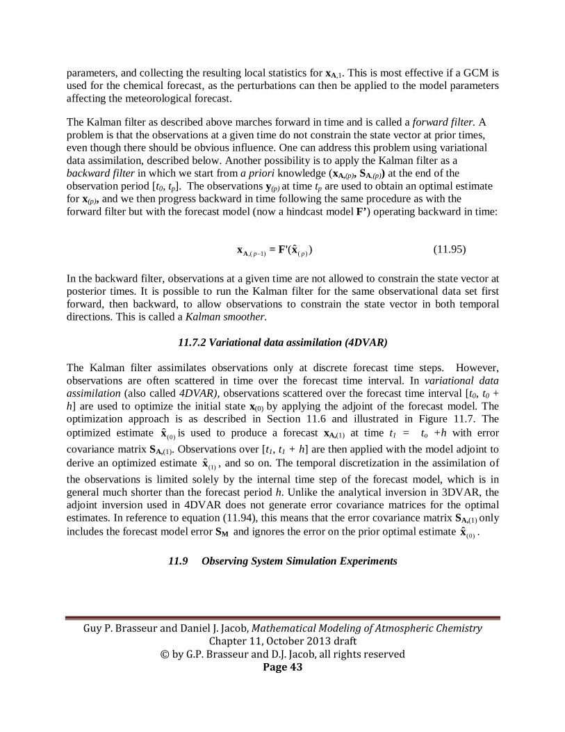
Guy P. Brasseur and Daniel J. Jacob, Mathematical Modeling of Atmospheric Chemistry Chapter 11, October 2013 draft
© by G.P. Brasseur and D.J. Jacob, all rights reserved Page 43
parameters, and collecting the resulting local statistics for xA,1. This is most effective if a GCM is used for the chemical forecast, as the perturbations can then be applied to the model parameters affecting the meteorological forecast.
The Kalman filter as described above marches forward in time and is called a forward filter. A problem is that the observations at a given time do not constrain the state vector at prior times, even though there should be obvious influence. One can address this problem using variational data assimilation, described below. Another possibility is to apply the Kalman filter as a backward filter in which we start from a priori knowledge (xA,(p), SA,(p)) at the end of the observation period [t0, tp]. The observations y(p) at time tp are used to obtain an optimal estimate for x(p), and we then progress backward in time following the same procedure as with the forward filter but with the forecast model (now a hindcast model F’) operating backward in time:
,( 1) ( )ˆ( )p p−Ax = F' x (11.95)
In the backward filter, observations at a given time are not allowed to constrain the state vector at posterior times. It is possible to run the Kalman filter for the same observational data set first forward, then backward, to allow observations to constrain the state vector in both temporal directions. This is called a Kalman smoother.
11.7.2 Variational data assimilation (4DVAR) The Kalman filter assimilates observations only at discrete forecast time steps. However, observations are often scattered in time over the forecast time interval. In variational data assimilation (also called 4DVAR), observations scattered over the forecast time interval [t0, t0 + h] are used to optimize the initial state x(0) by applying the adjoint of the forecast model. The optimization approach is as described in Section 11.6 and illustrated in Figure 11.7. The optimized estimate (0)x is used to produce a forecast xA,(1) at time t1 = to +h with error covariance matrix SA,(1). Observations over [t1, t1 + h] are then applied with the model adjoint to derive an optimized estimate (1)x , and so on. The temporal discretization in the assimilation of the observations is limited solely by the internal time step of the forecast model, which is in general much shorter than the forecast period h. Unlike the analytical inversion in 3DVAR, the adjoint inversion used in 4DVAR does not generate error covariance matrices for the optimal estimates. In reference to equation (11.94), this means that the error covariance matrix SA,(1) only includes the forecast model error SM and ignores the error on the prior optimal estimate (0)x .
11.9 Observing System Simulation Experiments

Guy P. Brasseur and Daniel J. Jacob, Mathematical Modeling of Atmospheric Chemistry Chapter 11, October 2013 draft
© by G.P. Brasseur and D.J. Jacob, all rights reserved Page 44
Observation System Simulation Experiments (OSSEs) are standard tests conducted during the design phase of a major observing program such as a satellite mission. Their purpose is to determine the ability of the proposed measurements to deliver on the scientific objectives of the program. These objectives can often be stated in terms of improving knowledge of a state vector x by using the proposed observations y in combination with a state-of-science forward model to relate x to y. For example, we might want to design a satellite mission to measure CO2 concentrations in order to constrain CO2 surface fluxes, and ask what measurement precision is needed to improve the constraints on the fluxes beyond those achievable from CO2 concentration measurements at surface sites.
If the state vector is sufficiently small that an analytical solution to the inverse problem is computationally practical (section 11.5), then a first assessment of the viability of the proposed observing system should be made by characterizing the error covariance matrices SA and SO, and constructing the Jacobian matrix K of the forward model. From there we can calculate the averaging kernel matrix A and a posteriori error covariance matrix S as described in Section 11.5. The trace of A defines the DOFS of the observing system (Section 11.5.3), and analysis of the rows of A determines the ability of the observing system to retrieve the individual components of x (Box 11.2). Comparison of S to SA, for example by taking the ratios of the diagonal terms (error variances), measures the reduction in error from the observing system. However, results will tend to be over-optimistic because of the idealized treatment of observational errors (Section 11.5.1).
A more stringent and general test is to conduct an OSSE using two different forward models simulating the same period (Figure 11.11). For an observing system targeting atmospheric composition these might be two independent CTMs: CTM 1 and CTM 2. The CTMs must both be state-of-science but otherwise as different as possible, so that difference between the two provides realistic statistics of the forward model error εM. In particular, they should use different assimilated meteorological data sets for the same period. We take CTM 1 as representing the “true” atmosphere, with “true” values of the state vector x generating a “true” 3-D field of atmospheric concentrations to be sampled by the observing system. We sample this “true” atmosphere with the observational characteristics of the proposed system including observation coverage, schedule, and random instrument and representation errors. This generates an ensemble of synthetic observations y over the time period. We then use CTM 2 as forward model over the same time period, starting from an a priori estimate (xA, SA) for the state vector and using the synthetic observations y to achieve an optimal estimate x . Analysis of the a posteriori differences x - x relative to the a priori differences xA – x provides an objective measure of the value of the observing system for constraining x.

Guy P. Brasseur and Daniel J. Jacob, Mathematical Modeling of Atmospheric Chemistry Chapter 11, October 2013 draft
© by G.P. Brasseur and D.J. Jacob, all rights reserved Page 45
Figure 11.11 Observing System Simulation Experiment (OSSE) for atmospheric composition using two independent CTMs. CTM 1 is taken to describe the “true” atmosphere, and CTM 2 is taken as the forward model for the inversion.