ESA SP-1233 (4)July 1999

Reports for Mission SelectionTHE FOUR CANDIDATE EARTH EXPLORER CORE MISSIONS

Atmospheric Dynamics Mission

ESA SP-1233 (4) – The Four Candidate Earth Explorer Core Missions –ATMOSPHERIC DYNAMICS_________________________________________________________________

Report prepared by: Earth Sciences DivisionScientific Co-ordinator: Paul Ingmann

Earth Observation Preparatory ProgrammeTechnical Co-ordinator: Joachim Fuchs

Cover: Richard Francis & Carel Haakman

Published by: ESA Publications Divisionc/o ESTEC, Noordwijk, The NetherlandsEditor: Bruce Battrick

Copyright: © 1999 European Space AgencyISBN 92-9092-528-0

Price: 70 DFl

3

CONTENTS

1 INTRODUCTION................................................................................................................................ 5

2 BACKGROUND AND SCIENTIFIC JUSTIFICATION............................................................... 9

2.1 GLOBAL WIND PROFILE MEASUREMENTS FOR CLIMATE AND NWP........................................ 92.2 THE NEED FOR ATMOSPHERIC WIND FIELDS FOR ATMOSPHERIC ANALYSES ......................... 102.3 POTENTIAL IMPROVEMENT OF NWP BY ENHANCED WIND OBSERVATIONS ........................... 142.4 THE NEED FOR ATMOSPHERIC WIND FIELDS FOR CLIMATE STUDIES...................................... 222.5 FUTURE STUDIES AND PERSPECTIVES AIMING AT IMPROVING THE WIND FIELD KNOWLEDGE

IN THE POST-2000 TIME FRAME ................................................................................................ 312.6 CONCLUSIONS ON NWP AND CLIMATE STUDIES ...................................................................... 33

3 RESEARCH OBJECTIVES ............................................................................................................. 35

3.1 MISSION OBJECTIVES ................................................................................................................. 353.2 NUMERICAL WEATHER PREDICTION ......................................................................................... 363.3 CLIMATE..................................................................................................................................... 373.4 ADDITIONAL OBSERVATIONS .................................................................................................... 39

4 OBSERVATIONAL REQUIREMENTS ........................................................................................ 41

4.1 INTRODUCTION........................................................................................................................... 414.2 METEOROLOGICAL ANALYSIS ................................................................................................... 424.3 COVERAGE REQUIREMENTS....................................................................................................... 464.4 QUALITY OF OBSERVATIONS ..................................................................................................... 484.5 RELIABILITY AND DATA AVAILABILITY.................................................................................... 524.6 CONCLUSION .............................................................................................................................. 53

5 MISSION ELEMENTS ..................................................................................................................... 57

5.1 INTRODUCTION........................................................................................................................... 575.2 INSTRUMENTS AND DATA .......................................................................................................... 575.3 ATMOSPHERIC ANALYSES AND NWP FORECASTS ................................................................... 61

6 SYSTEM CONCEPT......................................................................................................................... 63

6.1 FROM MISSION TO SYSTEM REQUIREMENTS............................................................................. 636.2 MISSION DESIGN AND OPERATIONS .......................................................................................... 666.3 THE ALADIN INSTRUMENT ...................................................................................................... 736.4 THE SATELLITE........................................................................................................................... 956.5 THE LAUNCHER........................................................................................................................1136.6 THE GROUND SEGMENT...........................................................................................................115

7 DATA PROCESSING AND VALIDATION................................................................................121

7.1 INTRODUCTION.........................................................................................................................1217.2 SPECTRA AND DOPPLER FREQUENCIES ...................................................................................1237.3 QUALITY CONTROL..................................................................................................................1247.4 IMPORTANCE OF CLOUDS.........................................................................................................1267.5 DISTRIBUTION AND ARCHIVING...............................................................................................1277.6 GEOPHYSICAL PROCESSING CENTRE.......................................................................................1277.7 CONCLUSIONS...........................................................................................................................129

8 MISSION PERFORMANCE..........................................................................................................131

8.1 INTRODUCTION.........................................................................................................................1318.2 PERFORMANCE IN CLEAR AIR..................................................................................................1338.3 THE IMPACT OF CLOUDS ..........................................................................................................1348.4 USEFULNESS FOR NWP............................................................................................................1378.5 USEFULNESS FOR CLIMATE STUDIES.......................................................................................1388.6 OTHER ELEMENTS PROVIDED BY THE ADM ...........................................................................1408.7 CONCLUSIONS...........................................................................................................................141

9 PROGRAMMATICS.......................................................................................................................143

9.1 DEVELOPMENT APPROACH ......................................................................................................1439.2 HERITAGE, CRITICAL AREAS AND RISKS ................................................................................1459.3 RELATED MISSIONS, INTERNATIONAL CO-OPERATION POSSIBILITIES AND TIMELINESS ......1479.4 ENHANCEMENT OF CAPABILITIES AND APPLICATIONS POTENTIAL........................................148

REFERENCES ...........................................................................................................................................149

GLOSSARY ................................................................................................................................................153

ACKNOWLEDGEMENTS.......................................................................................................................157

5

‘Hurricane force winds raged across Britain onChristmas Eve and yesterday leaving five people dead,five French fishermen feared drowned in the Irish Sea,thousands of people without power and scores of roadsblocked by fallen trees and masonry.

As the emergency services battled to cope, a fresh waveof storms with winds gusting up to 70 mph swept acrossLondon and much of southern England last night.’

(from ‘The Times’, 26 December 1997)

1 Introduction

The ‘ESA Living Planet Programme’ (ESA, 1998) describes the plans for theAgency's new strategy for Earth Observation in the post 2000 time frame. It marks anew era for European Earth Observation based on smaller more focused missions anda programme that is user driven, covering the whole spectrum of interests rangingfrom scientific research-driven Earth Explorer missions through to application-driven

Earth Watch missions. The user community is therefore now able to look forward to aprogramme of more frequent but very specific missions directed at the fundamentalproblems of Earth system sciences.

Out of the nine Earth Explorer core missions identified in ESA SP-1196 (1-9), fourcore missions were selected for Phase-A studies, which began in June 1998, namely:the Land-Surface Processes and Interactions Mission; the Earth Radiation Mission; theGravity Field and Steady-State Ocean Circulation Mission; and the AtmosphericDynamics Mission. The Phase-A studies were all completed in June 1999.

This ‘Report for Mission Selection’ for the Atmospheric Dynamics Core Mission(ADM) was prepared by a Core Mission Drafting Team consisting of four members ofthe ADM Advisory Group (ADMAG); E. Källén, J. Pailleux, A. Stoffelen andM. Vaughan. They were supported by the other members of the ADMAG, namelyL. Isaksen, P. Flamant, and W. Wergen. The technical content of the report (notablyChapter 6) has been compiled by the Executive based on inputs provided by theindustrial Phase-A contractor. Others who, in various ways, have contributed to thereport are listed in the Acknowledgements.

The primary aim of the Earth Explorer Atmospheric Dynamics Mission is to provideimproved analyses of the global three-dimensional wind field by demonstrating thecapability to correct the major deficiency in wind-profiling of the current GlobalObserving System (GOS) and Global Climate Observing System (GCOS). The ADMwill provide the wind-profile measurements to establish advancements in atmosphericmodelling and analysis. There is an intimate link between progress in climatemodelling and progress in numerical weather prediction (NWP) as our understandingof the atmosphere is largely based on the experience of operational weather centres.Long-term data bases are being created by NWP data assimilation systems to serve theclimate research community. It is widely recognised therefore that the impact of a newglobal atmospheric observing system on our understanding of atmospheric dynamicsshould be evaluated primarily in the context of operational weather forecasting.

New insights into the atmosphere through the provision of wind profiles are expectedfor NWP, but also for climate research. The ADM is addressing one of the main areasdiscussed under Theme 2 of the ‘ESA Living Planet Programme’ (ESA, 1998).Although there are several ways of measuring wind from a satellite, only the activeDoppler Wind Lidar (DWL) has the potential to provide the requisite data globally. Itis the only candidate so far that can provide direct observations of wind profiles. Inaddition, a DWL will not only provide wind data, but also has the potential to provideancillary information on cloud top heights, vertical distribution of cloud, aerosolproperties, and wind variability as by-products.

This Report for Mission Selection for the ADM, together with those for the other threeEarth Explorer Core Missions, is being circulated amongst the Earth Observation

7

research community in preparation for The Four Candidate Earth Explorer CoreMissions Consultative Workshop in Granada (Spain) in October 1999.

Following this introduction, the report is divided into eight chapters:

1) Chapter 2 addresses the background and provides the scientific justification forthe mission set in the context of issues of concern and the associated need toadvance current scientific understanding. The chapter identifies the problemand gives the relevant background. It provides a review of the current statusand the clear identification of the ‘gaps’ in knowledge. In so doing, it providesa clear identification of the potential ‘delta’ this mission would provide.

2 ) Drawing on these arguments, Chapter 3 discusses the importance of thescientific objectives. It identifies the need for such observations by comparingthe data that will be provided by this mission with that available from existingand planned data sources, highlighting the unique contribution of the mission.

3) Chapter 4 focuses on mission requirements comparing ‘current practice’ withthe novelty of the mission and derives, in the context of the scientificobjectives, the mission specific observational requirements. It confirms that theADM, with its well-balanced measurement capabilities, would be unique inobtaining a new and quantitative understanding of the Earth’s wind field.

4) Chapter 5 provides an overview of the various mission elements such as spaceand ground segments and external sources laying the foundations for missionimplementation.

5) Drawing on Chapter 5, Chapter 6 provides a complete summary description ofthe proposed technical concept (space and ground segments). The technicalmaturity of the concept is illustrated by the way it meets the observationalrequirements addressed in Chapter 4.

6 ) Chapter 7 outlines the envisaged data processing scheme. It includes adescription of the algorithms proposed. The processing chain is described,clearly demonstrating the feasibility of transforming the raw data viacalibration and validation into the requisite geophysical products.

7) Drawing on Chapters 5 to 7, a comparison of expected mission performanceversus performance requirements (Chapter 4) is provided in Chapter 8. Thisdraws on the main findings of the previous chapters, complemented by resultsof an end-to-end simulation tool, to demonstrate that the expected missionperformance is indeed capable of meeting (a) the observational requirements(Chapter 4) and (b) the ADM scientific objectives as outlined in Chapter 2.

8 ) Programme implementation, including risks, development schedule andinternational collaboration, is discussed in Chapter 9. In particular, drawing onthe previous chapters, Chapter 9 discusses the ADM in the context of otherrelated missions. It is finally concluded that the proposed launch time in the2004 time-frame would be very timely for the scientific community.

9

2 Background and Scientific Justification

2.1 Global Wind Profile Measurements for Climate and NWP

Reliable instantaneous analyses and longer term climatologies of winds are needed toimprove our understanding of atmospheric dynamics and the global atmospherictransport and the cycling of energy, water, aerosols, chemicals and other airbornematerials. However, improvement in analysing global climate, its variability,predictability and change requires measurements of winds throughout the atmosphere.In order to do so, it is a pre-requisite to improve NWP as progress in climate-relatedstudies is intimately linked to progress in operational weather forecasting. The WorldMeteorological Organisation (WMO) states in their recent evaluation of userrequirements and satellite capabilities that for global meteorological analysesmeasurement of wind profiles remains most challenging and most important (WMO,1998).

After several decades of observations from space, direct measurements of the fullyglobal, three-dimensional wind field remain elusive. Deficiencies, including coverageand frequency of observations, in the current observing system are impeding progressin both climate-related studies and operational weather forecasting. There is a clearrequirement for a high-resolution observing system for atmospheric winds with fullglobal coverage.

At present, our information on the three-dimensional wind field over the oceans, thetropics and the southern hemisphere is indirect. It is severely limited by having to relyon mainly space-borne observation of the mass field and geostrophic adjustmenttheory. Improvements in the available wind data are needed urgently if we are toexploit fully the potential of recent advances in climate prediction and NWP andcontinue to make significant progress in the field.

There is a synergy between advances in climate-related studies and those in NWP.Indeed, climate studies are increasingly using analyses of atmospheric (and other)fields from data assimilation systems designed originally to provide initial conditionsfor operational weather forecasting models. Understanding of the atmosphere and itsevolution is based to a large extent on the analysed fields from continuous dataassimilation carried out at operational weather centres, so that progress in climateanalysis is closely linked to corresponding progress in NWP. In line with this,extended atmospheric reanalysis projects (ERA15, ERA40, NCEP) are being carriedout to provide the climate and research community with consistent data sets. Theanalysis of the atmospheric flow is further of prime interest for studies on atmosphericcomposition and chemistry. In presenting the scientific justification for therequirement for better global measurements of atmospheric winds, given theimportance of data assimilation, first their importance for NWP is considered,followed by a discussion of the corresponding requirement for climate studies andatmospheric research. Before concluding this chapter, the role of atmospheric

dynamics for atmospheric chemistry is discussed. The atmospheric requirements areput in perspective with other requirements of the Earth’s system in ESA (1998) wherethe hierarchy of Earth system models is also described in general.

2.2 The Need for Atmospheric Wind Fields for Atmospheric Analyses

2.2.1 Background

Analyses of the atmospheric state are needed for a wide range of climate-relatedstudies and for NWP. Such meteorological analyses provide a complete three-dimensional picture of the dynamical variables of an atmospheric model at a particulartime.

In an operational data assimilation system, these analyses are produced continuouslyand in sequence. In NWP, medium-range forecasts, which predict the evolution of theglobal atmosphere typically from four to ten days ahead, are generally started twice aday, at 00 and 12 UTC. Often embedded in the global models are high-resolution,limited-area models for high-resolution analyses and for short-range predictions up to2 to 3 days ahead, which are started from initial times usually only 6 or 3 hours apart.The most common prognostic model variables are: the horizontal wind components,temperature, humidity and surface pressure. In the future, more and more atmosphericmodels will require additional initial values, such as cloud water, cloud ice, cloudamount, turbulent kinetic energy and densities of various constituents, such as ozoneand aerosol.

In order to obtain an appropriate description of the atmosphere, a compositeoperational observing system has been established under the auspices of the WMO.The World Weather Watch (WWW) of the WMO is a well-established system co-ordinating the operational provision of meteorological data. It consists of a number ofdifferent observing platforms which take observations either at pre-specified times(synoptic hours) or quasi-continuously. They can be grouped further into in-situ orremote-sensing measurements. They either provide information for one level only(surface or upper-air) or give profiles for a number of levels in the vertical.

2.2.2 Data Deficiencies

The different types of observations currently available and constituting the GlobalObserving System (GOS) are documented in full detail in ESA (1996). They can beclassified in the following way:

• Surface data – they are the synoptic reports from land stations and ships, the(moored and drifting) buoys, and also the scatterometer winds from satellites

11

(such as ERS). They are all single level data, and cannot provide anyinformation on atmospheric profiles.

• Single-level upper-air data – mainly aircraft reports and cloud motion windsderived from geostationary satellite imagery. More and more aircraftobservations (wind and temperature) are being made during ascent and descentphases, thus tending to become ‘multi-level’. Their main deficiency is the poordata coverage: observations are provided only along the air routes and theynever provide any profile-type information over the oceans. Satellite cloud (orwater vapour) winds are derived from the motion of some targets like clouds,assuming that this target is advected by the atmospheric flow; an intrinsicassumption which is not always true. Compared with other single-level data,they have another deficiency: the significant uncertainty in knowledge of thelevel. Finally they are available only in a latitude belt around the equator: 50˚Sto 50˚N.

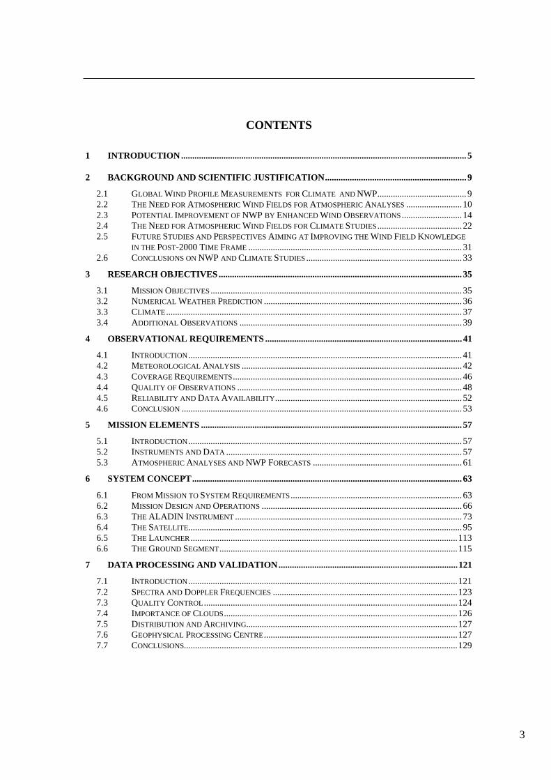
• Multi-level upper-air data – mainly the radiosondes (Fig. 2.1) and the polarorbiting sounder data (Fig. 2.2). Satellite sounders provide global coveragewith radiance data, which can only be used indirectly for the definition of themass field (temperature and humidity). Radiosondes are the only currentobserving system providing vertical profiles of the wind field, but they areavailable mainly from the continents in the northern hemisphere. Theradiosonde network has been gradually deteriorating in recent years. As such,three-dimensional wind measurements remain relatively scarce.

Figure 2.1. The radiosonde network – radiosonde/pilot ascents containing windprofile information that were available at DWD for the 6-hour time window centredaround 12 UTC, 28 April 1999. This is a typical distribution and wind profileinformation is generally lacking over all ocean areas.

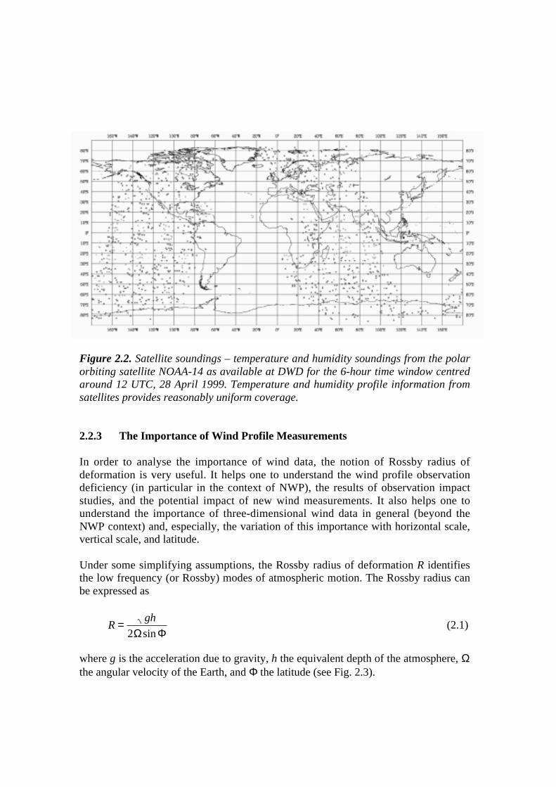
Figure 2.2. Satellite soundings – temperature and humidity soundings from the polarorbiting satellite NOAA-14 as available at DWD for the 6-hour time window centredaround 12 UTC, 28 April 1999. Temperature and humidity profile information fromsatellites provides reasonably uniform coverage.

2.2.3 The Importance of Wind Profile Measurements

In order to analyse the importance of wind data, the notion of Rossby radius ofdeformation is very useful. It helps one to understand the wind profile observationdeficiency (in particular in the context of NWP), the results of observation impactstudies, and the potential impact of new wind measurements. It also helps one tounderstand the importance of three-dimensional wind data in general (beyond theNWP context) and, especially, the variation of this importance with horizontal scale,vertical scale, and latitude.

Under some simplifying assumptions, the Rossby radius of deformation R identifiesthe low frequency (or Rossby) modes of atmospheric motion. The Rossby radius canbe expressed as

Rgh

=2Ω Φsin

(2.1)

where g is the acceleration due to gravity, h the equivalent depth of the atmosphere, Ωthe angular velocity of the Earth, and Φ the latitude (see Fig. 2.3).

13

Figure 2.3. Rossby radius of deformation for a latitude of 45° as a function ofhorizontal scale and equivalent depth. Open area denotes the range within which thewind field dominates the atmospheric dynamics, and three-dimensional windmeasurements are important.

For horizontal scales smaller than R, the wind is the essential information and theatmospheric mass field adjusts to it. For horizontal scales larger than R, the windadjusts to the mass field. R also depends on the vertical scale of the atmosphericfeature that is being considered (equivalent depth):

• At the equator, R goes to infinity, so in the tropics information on the windfield is essential as it governs tropical dynamics. In the extra-tropics, wind dataare the primary source of information for small horizontal scale features(length scales L << R) and deep vertical structures.

• Mass field information is important for large horizontal scale features (L >> R)and shallow vertical structures.

Between these two extremes, there is a wide range where both mass and wind data arerequired.

From this simple theoretical analysis (see ESA, 1996), it is expected that wind profileobservations have a major impact on forecasting in the tropics and the prediction ofsmall-scale structures in the extra-tropics (deriving small-scale winds from height field

observations does not reflect the true dynamics). Having wind profile observations inthe tropics would help considerably in advancing understanding of tropical dynamicsand, probably, the forecasting of severe events such as tropical cyclones.

In the extra-tropics, the availability of more wind profile data is expected to lead tocapturing, much better and much earlier, of initial instabilities of the flow in the stormtracks, and subsequently to improve considerably forecasts of storm developments(especially the intense ones). Even for large-scale structures in the extra-tropics, whenthe wind field adjusts to the height data, wind data are still useful for at least tworeasons. Firstly, because for large planetary scales the geostrophic relation betweenmass and wind is not valid. Secondly, when deriving the wind field from observedheight, relatively small observation errors on the height can lead to significant errorsin the derived wind. Therefore, it is important to measure the three-dimensional windfield directly.

2.3 Potential Improvement of NWP by Enhanced Wind Observations

2.3.1 Implication of Data Deficiencies for NWP

A typical NWP model contains many more variables in its initial state than theaccumulation of all the pieces of data from the observations accumulated over a 6-hour period (typical for most of the operational data assimilation systems; see ESA,1996 for a detailed quantitative assessment). This means that NWP is a seriouslyunder-determined initial-value problem. With increasing computer power andincreased resolution, it is likely to become more and more under-determined, in spiteof new satellite instruments bringing higher and higher data volumes (ATOVSsounder replacing TOVS in 1999 with more channels; plans for a new generation ofsounders giving more details on the vertical distribution of temperature and humidity).

Modern data assimilation systems are quite efficient in making optimal use of thecurrent operational observations. They help in reducing the under-determinationproblem by bringing in additional statistical and dynamical information (seeMeteorological Society of Japan (1997) for an overview of the data assimilationalgorithms and problems, and Rabier et al. (1998a) for the description of a modernoperational data assimilation system, based on a four-dimensional variationalassimilation scheme, 4D-Var). Such a scheme is likely to be used in many NWPcentres in a few years and is currently the natural candidate to assimilate wind data.

However, despite the sophistication of modern data assimilation schemes, largeuncertainties are left in some wide areas on the globe, for the wind field itself, forother fields that are important for NWP, and for diagnosed integrated quantities whichare important to understand the climate. Some of these uncertainties are documentedin ESA (1996).

15

Figure 2.4. Analysis and forecasts of the ‘Christmas Eve Storm’ – Mean Sea LevelPressure (MSLP) maps illustrating the ‘Christmas Eve Storm’ which hit the BritishIsles on 24 December 1997, 12 UTC, after a rapid development from the middle of theAtlantic Ocean (Courtesy A. Persson, ECMWF). – Top left: manual analysis for 24 December 1997, 12 UTC; – Top right: ECMWF 12-hour forecast from 24 December 1997, 00 UTC (valid 12 UTC); – Bottom: equivalent 12-hour forecasts from the UKMO (left) and the DWD (right)

models.

Even at very short range, NWP models can be hit by severe failures which, although itcannot be always proven, are suspected to be due to a lack of meteorologicalobservations in some areas which are critical for the initial state of these models. Oneexample is the storm of 24 December 1997 (now called ‘Christmas Eve Storm’, seeChapter 1), which deepened very quickly in the middle of the Atlantic Ocean on the23rd and 24th of December 1997, then hit Ireland and the Irish Sea in the afternoon ofthe 24th, and finally the North of England and Scotland. The short-term forecasts ofthe storm from all operational models were poor, even at very short range as illustratedin Figure 2.4. Figure 2.5 shows the 36 hour forecast produced by the Frenchoperational model (ARPEGE) valid also for 24 December, 12 UTC: it missed the Irishstorm and developed another one which was about 1000 km to the southwest (this canbe interpreted as an enormous phase error). It has to be noted that even at very

Figure 2.5. Forecast using the Modified Operational Model of Météo-France –36-hour MSLP forecast valid 24 December 1997, 12 UTC (top). The sensitivity of thestorm forecast with respect to a modification of the initial conditions (on 23 December1997, 00 UTC) has been computed using a modified forecast model (CourtesyG. Hello, Météo-France).

17

short range (12-hour), the operational models produce extremely poor forecasts of thestorm (the pressure error near the centre of the low exceeds 20 hPa). In most of theoperational assimilation systems, the (computer-based) objective MSLP analysisunderestimates the depth of the low, because the available observations were sodifferent from the very poor first guess that they were rejected in the analysis. Thisexplains why a manual analysis (rather than an objective one) has to be shown in thisfigure.

The examination of the different operational analyses on the 22nd and 23rd, togetherwith the satellite imagery, indicates that these analyses were often unable to catchaccurately the different weather systems (cyclogenesis, developing waves, and theirprecursors), presumably because of rapid cross-Atlantic circulation, rapid baroclinicdevelopments and insufficient data coverage.

A modified version of the ARPEGE model was then used to compute three-dimensional sensitivity fields, which indicate where and to what extent the initialconditions should have been modified on 23 December, 00 UTC, in order to predictcorrectly the storm at 36-hour range for 24 December, 12 UTC. The outcome of thisexample of sensitivity study is that a small change in the middle of the Atlantic (seetemperature modification in Fig. 2.5 – bottom), for the three-dimensional thermo-dynamical structure of the analysis would have converted this 36-hour forecast failureinto a good storm forecast; see Hello et al. (1999). A simple calculation shows that thissmall change corresponds to 1 or 2 ms-1 on the wind shear taken between 700 and850 hPa (for example) in some areas of the middle Atlantic. It is then likely that agood three-dimensional coverage of observations in this area would have improved theforecast considerably. More generally one can reasonably think that a good three-dimensional coverage of observations over the North Atlantic would have improvedconsiderably the forecasts over the North Atlantic and Europe during this few days'period before Christmas 1997, including the dangerous meteorological event of the‘Christmas Eve Storm’.

The requisite wind profiles would be available from the ADM meeting the requirementfor high accuracy wind observations.

2.3.2 OSE and OSSE: Principles, Limitations and Some General Results

In order to assess the impact of wind profile data on NWP in a way which is morequantitative than the previous theoretical developments in Section 2.2, ObservingSystem Experiments (OSE) and Observing System Simulation Experiments (OSSE)have been run in NWP for at least twenty years. OSE are impact studies carried outwith existing observations: two parallel data assimilations are carried out, with andwithout the observing system to be evaluated; resulting analyses and subsequentforecasts are then compared. OSSE are similar to OSE except the observations to betested are simulated rather than real: simulated observations are produced from an

NWP model integration assumed to be the ‘known truth’ and usually called the ‘naturerun’. For a quantitative assessment of a non-existing observing system like the globalwind profiles, which may be produced by a space Doppler lidar in the next decade,OSSE are required.

WMO (1997) gives an overview of the impact of existing operational observingsystems on the forecast, through a synthesis of OSE carried out until April 1997. Italso presents (paper by Atlas in WMO, 1997) the details of the OSSE methodologyand its limitations, which have to be kept in mind when evaluating the results. Itunderlines ‘the need for providing observations from a realistic nature run, forsimulating properly the observation errors, for calibrating properly all the componentsof the OSSE, and for using an assimilating model different enough from the modelproducing the nature run’. Finally, from old OSSE results, it indicates a significantpotential for further improvement from a space-based wind profiler, also with respectto the TOVS observing system. The OSE run by Graham et al. (ibid) indicates that, onaverage, for predicting cyclogeneses over the North Atlantic and Europe, wind profileobservations are somewhat more important than temperature profile observations.

Table 2.1 (extracted from WMO, 1997) shows a summary of the impact of differentobservation types over the northern-hemisphere extratropics. The values given foreach observation type represent results from impact studies carried out during theperiod 1994-97. The results are expressed in terms of maximum gain in large-scaleforecast skill at short and medium range. This table is only meant as a rough guide.The magnitudes of the impact depend, for example, upon the model and assimilationscheme used and the observed variables. Therefore, generalisation of impactmagnitudes must be treated with caution. However, it is clear that the northern-hemisphere radiosonde network stands out as being especially important (presumablybecause it is the only system providing accurate profiles of wind and temperature on asignificant portion of the hemisphere).

Neutral toFew Hours

Up to 1/4day

0.5 day 1.0 days 1.5 days

TOVSCloud motion windsSondesAircraft (*)Scatterometer

Note: (*) impact only locally

Table 2.1. Impact of different types of observation on forecast skill (from WMO,1997). Vertical soundings that include wind observations have large impact.

19

2.3.3 Results of Recent Studies on the Impact of Wind Profiles

A very good estimate of the potential impact of a future space-based Doppler windlidar system can be obtained by running an OSE evaluating the impact of real windprofile observations available on a data-dense area like North America. This was doneby Cress (1999) using the Deutscher Wetterdienst global data assimilation andforecasting system. Figure 2.6 shows the drastic degradation of the forecasts over theNorth Atlantic and Europe produced by the withdrawal of radiosonde and aircraftwind profiles over North America (USA plus Canada). The start date of the forecast is30 January 1998, 12 UTC and the differences are for the initial state (a) and after3.5 days (b), 5.5 days (c) and 7.5 days (d) forecast time. The detailed evaluation of thescores show that the forecast is degraded by about 24 hours.

Figure 2.6. Illustration of degradation of forecasts without wind profiles – differencesin the 500 hPa geopotential height field between a forecast using all availableobservations and experiments not using radiosonde, pilot and aircraft wind data overthe United States and Canada. Contour interval is 20 m for a) and 40 m for b) to d)(from Cress, 1999).

In a recent OSSE performed in Germany as a continuation of this OSE, it was shownthat a system providing only a small number of wind profiles in place of the

conventional wind observations over North America would recover more than half ofthis forecast degradation. Figure 2.7 (from the same study) illustrates that even atforecast range 0 (model initial state), systematically removing the North-Americanwind profiles produces wind uncertainties over almost the entire tropical area,indicating that the tropical flow is rather uncertain. This experiment provides a roughestimate of the potential impact of wind profile data available in a data sparse area ofthe size equivalent to North America. Forecasts started from the degraded analysisreduced the operational medium-range forecast skill by 20 hours.

Figure 2.7. Degradation of the global wind field – analysis of differences in thegeopotential height and wind field at 500 hPa between an 11 day long assimilation notusing wind profile observation from radiosondes, pilots and aircraft over the UnitedStates and Canada and the control assimilation using all observations. The differenceis valid for 30 January 1998, the contour interval for the height field is 20 m (fromCress, 1999).

Another interesting OSE has been carried out by Isaksen (Ingmann et al., 1999) withthe 1997 ECMWF global data assimilation and forecasting system. It evaluates theimpact of all the radiosonde wind profiles above the planetary boundary layer (PBL)versus the impact of the radiosonde mass profiles (geopotential height) and also that ofall the available radiosonde information. The results expressed in terms of averageskill scores are displayed in Figure 2.8. The impact is found to be much larger than theimpact of any single-level data observing system, and equivalent to a big portion ofthe total radiosonde network impact, which includes temperature and humidityinformation.

21

An ECMWF model nature run was used to produce an OSSE data base simulating ascenario in which wind data (assumed from a DWL) were available (Stoffelen andMarseille, 1998). In the same reference, one can read about the analysis of the database: ‘Vertical wind-shear is only weakly correlated to cloud coverage, implying thatshear is well observed from space; we conclude that such data may bring an importantimprovement to the forecast of cyclogenesis, since it would provide wind profiles inotherwise data-sparse regions’.

Figure 2.8. Results of assimilation studies – carried out with ECMWF’s three-dimensional variational system for the Northern Hemisphere for a) full set ofobservations (red line), b) no use of TEMP/PILOT (brown line), c) no use ofTEMP/PILOT winds above 775 hPa (blue line), d) no use of TEMP/PILOTtemperature profiles but only winds (green line).

This data base has been used by Cardinali et al. (1998) to carry out an OSSE with aversion of the Météo-France global model at low resolution and 4-DVar assimilationscheme. It was shown that near a trough situated over the Pacific Ocean, to the west ofthe Canadian coast, the availability of wind profiles helped considerably the windanalysis (confirmation of the finding of Stoffelen and Marseille, 1998). In Cardinali etal. (1998), three different scenarios have been intercompared:

• ONLYLOS: only DWL data have been assimilated

• CONTROL: corresponding roughly to current observing systems; notehowever that TOVS data were not used in CONTROL

• LIDAR: DWL data have been added to the observations of CONTROL.

Table 2.2 shows the performance of the three different scenarios in terms of analysiserrors (mean and standard deviations of the differences to the nature run), for threedifferent areas and three different levels. It is clear that the LIDAR scenario is much

improved compared to CONTROL, especially in the Southern Hemisphere and in thetropics.

Area Level (hPa) ONLYLOS CONTROL LIDARMean St. Dev. Mean St. Dev. Mean St. Dev.

NorthernH.

850500250

3.564.776.03

2.152.953.64

2.633.203.28

1.822.222.20

2.392.883.06

1.541.872.01

Tropics 850500250

3.384.486.18

2.512.693.99

3.043.965.29

2.132.363.39

2.603.204.20

1.741.952.62

SouthernH.

850500250

3.764.516.98

2.342.704.59

3.895.737.62

3.583.605.08

2.743.484.76

1.702.063.16

Table 2.2. Mean and standard deviations of the analysis errors (expressed in ms-1 asthe module of the vector ‘Analysis – Truth’) for three OSSE scenarios at threedifferent levels and in three different areas over the globe (from Cardinali et al.,1998). A DWL well complements the existing GOS in improving atmospheric analyses.

The results of OSEs and OSSEs carried out indicate that improved wind profileobservations as will be provided by the ADM would have a large impact over differentregions of the globe.

2.4 The Need for Atmospheric Wind Fields for Climate Studies

2.4.1 Background

Climate-change issues have received substantial attention in recent years due to theincreasing awareness that human activities may substantially modify the future climateof the Earth. The globally averaged temperature has increased by about 0.6 degreesCelsius over the past hundred years and 1998 was the warmest year recorded oninstrumental temperature record covering the last 150 years. These facts and otherpieces of evidence suggest that an increased greenhouse effect due to human activitiesis starting to influence the global climate system. A very important question is thus toassess how a further future increase in greenhouse gases may affect this system. Themost effective tools available to answer such questions are global and regional climatemodels, which to a very large extent resemble the corresponding NWP models. All thebenefits of wind data discussed in the previous section relating to NWP models arealso relevant to circulation models used for climate studies as both model types arebased on the same physical and numerical principles.

23

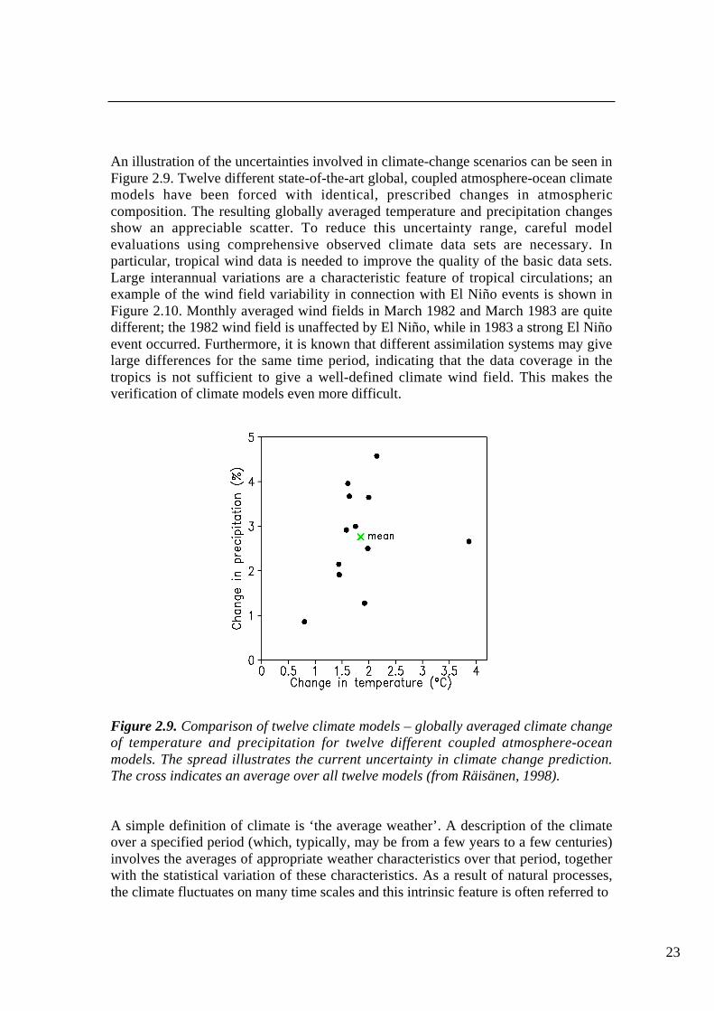
An illustration of the uncertainties involved in climate-change scenarios can be seen inFigure 2.9. Twelve different state-of-the-art global, coupled atmosphere-ocean climatemodels have been forced with identical, prescribed changes in atmosphericcomposition. The resulting globally averaged temperature and precipitation changesshow an appreciable scatter. To reduce this uncertainty range, careful modelevaluations using comprehensive observed climate data sets are necessary. Inparticular, tropical wind data is needed to improve the quality of the basic data sets.Large interannual variations are a characteristic feature of tropical circulations; anexample of the wind field variability in connection with El Niño events is shown inFigure 2.10. Monthly averaged wind fields in March 1982 and March 1983 are quitedifferent; the 1982 wind field is unaffected by El Niño, while in 1983 a strong El Niñoevent occurred. Furthermore, it is known that different assimilation systems may givelarge differences for the same time period, indicating that the data coverage in thetropics is not sufficient to give a well-defined climate wind field. This makes theverification of climate models even more difficult.

Figure 2.9. Comparison of twelve climate models – globally averaged climate changeof temperature and precipitation for twelve different coupled atmosphere-oceanmodels. The spread illustrates the current uncertainty in climate change prediction.The cross indicates an average over all twelve models (from Räisänen, 1998).

A simple definition of climate is ‘the average weather’. A description of the climateover a specified period (which, typically, may be from a few years to a few centuries)involves the averages of appropriate weather characteristics over that period, togetherwith the statistical variation of these characteristics. As a result of natural processes,the climate fluctuates on many time scales and this intrinsic feature is often referred to

a)

b)

Figure 2.10. Divergent wind field at 150 hPa – monthly mean divergent winds overthe Pacific region for the months of March 1982 (a) and March 1983 (b). In (a) thereis a divergent outflow over the Indonesian region which is associated with normaltropical heating. In (b) the outflow has moved to the Central Pacific and this shift isassociated with the El Niño event extending over 1982 and 1983.

25

as natural climate variability. In this report, the term ‘climate change’ refers to anychange in climate over time, whether this is due to natural variability or humanactivity or, indeed, is a consequence of both these causes.

Although the climate varies over a vast range of time scales, from inter-annual tomany thousands of years, two ranges are currently receiving particular attention. Theseare, firstly, the seasonal-to-interannual time-scale range and, secondly, the decadal-to-centennial time-scale range. These, particularly the latter, provide the focus for thissection of the report. Following brief comments on the general data requirements forcurrent studies involving these two time-scale ranges, this section discusses theparticular needs for wind data for climate studies, including atmospheric composition,with separate comments on tropospheric and stratospheric winds.

In the context of climate studies, one of the highest-priority concerns for better globalwind measurements has been expressed by the Scientific Steering Group of the GlobalEnergy and Water Cycle Experiment (GEWEX), a major component of the WorldClimate Research Programme (WCRP).

2.4.2 Seasonal-to-Interannual Variability and Predictability

Recent research has achieved significant progress in making credible predictions for afew seasons ahead for certain regions of the globe. Success to date has been mostevident for some tropical areas and has resulted from research conducted principallyunder the auspices of the WCRP, to understand the interactions of the tropical oceanand global atmosphere (TOGA) and the related large-scale ENSO (El Niño/SouthernOscillation) phenomenon.

Standard meteorological data sets are required to initialise and validate seasonal-to-interannual climate predictions. In this context, atmospheric wind is a keymeteorological variable, particularly in the tropics where reliable wind observationsare crucial as their inclusion in the NWP assimilation process strongly affects thelarge-scale features of the analysed tropical wind field. For example, westerly windbursts (WWB) or events (WWE) play an important role in the onset of El Niño byproviding a strong and irreversible forcing on the upper ocean. However, the causeand occurrence of these WWB in relation to the ambient tropical dynamics is poorlyknown.

Whilst the evidence for seasonal predictability is strongest in the tropics, there is nowalso growing evidence of some predictability in the extra-tropics. Global data,including atmospheric winds, are therefore required for a range of uses in connectionwith the investigation of seasonal variability and predictability, and the developmentand application of seasonal-to-interannual prediction techniques.

The ADM will provide the wind profiles needed to initialise models and validateseasonal-to-interannual predictions.

2.4.3 Decadal-to-Centennial Climate Variability and Predictability, IncludingModelling and Detection of Anthropogenic Climate Change

The prospect that the global climate may be modified by human influence has led tothe establishment of international programmes to monitor and increase theunderstanding of climate and to detect, attribute and predict climate change.Comprehensive observations of the climate system are recognised as being anessential component of these programmes and so the Global Climate ObservingSystem (GCOS) has been established to ensure that the observational needs forclimate are met in a co-ordinated and systematic manner.

In the current debate about climate change, it is evident that adequate information isnot available to answer fully the critical scientific questions. While manyobservational programmes are currently under way, systematic global observations ofkey variables, including atmospheric winds, are urgently needed to:

• monitor the climate and its variability at global, regional and more local scales,thereby enabling quantification of natural climatic fluctuations and extremeevents on a range of temporal and spatial scales and the detection of climatechange

• establish ‘fingerprints’ of climate change, which will allow not only detectionof change but also some attribution to its causes

• conduct diagnostic studies to document and understand better the behaviour ofthe climate system and its component parts, including studies of themechanisms of natural climate variability

• model climate and predict climate change.

Model-related climate studies require global observations for a number of reasons.Atmospheric wind data are required principally for the validation of the models, i.e. toassess the performance of models being used for climate simulation and prediction.Model behaviour is compared with that of the ‘observed’ climate, often leading tofurther development and improvement of the models. This applies not only to multi-decadal simulation and prediction, but also to the seasonal-to-interannual studiesdiscussed above.

The acquisition of systematic and comprehensive space-based global observationswith adequate coverage in space and time is essential to meet the above aims.However, in addition to the requirements for continuous, systematic data collection,special data are also needed in support of detailed research studies of a wide variety of

27

complex dynamical, physical and other processes that govern the state and evolutionof the climate system. Such specialised data sets are likely to need to be highlyresolved in time and space and may therefore need to be gathered for a limited periodonly. In particular, further progress in understanding and predicting global climatechange is critically dependent upon improvements in the ability to model energeticprocesses, as detailed in the scientific plan for GEWEX. The high priority attached towind data in support of GEWEX is discussed below.

The ADM will provide the systematic and comprehensive data needed to enablepredictions of climate change.

2.4.4 The Importance of Wind Data for Climate Studies

Climate research is highly dependent upon reliable global analyses of standardatmospheric variables, including winds throughout the atmosphere. These constitutethe basic data needed to infer more complicated quantities, such as the properties ofatmospheric transport and the surface fluxes of momentum, energy and mass, whichare not measured directly or routinely. Global coverage with optimal verticalresolution and representative horizontal spacing are the crucial requirements for manyclimate activities and so, as in the case of NWP (Section 2.2), space-basedobservations are particularly important in this context. Earlier expert studies havealready stressed the great importance of accurate vertical profiles of wind andtemperature which largely determine the quality of many of the other importantmeteorological fields. To provide such profiles in a consistent way over severaldecades for atmospheric scientists, re-analysis projects are carried out (ERA15, NCEP,ERA40).

Atmospheric data, including winds, are required to better understand the dynamics ofthe climate system and its natural variability. In particular, as implied above,atmospheric data are needed to monitor the current state of the climate, to detectchange and to validate the models that are used for seasonal forecasting, simulatingclimate and providing projections of climate change due to human activities. Relatedresearch, such as studies of the serious depletions of stratospheric ozone over theArctic and Antarctic, would also be much better served by the availability of globalwind data.

The main requirement is for long-term, consistent and representative global data sets,but there is also a call for shorter-period data sets to aid understanding through processand diagnostic studies. Better information is needed on the atmospheric circulation totry to attribute climate change to particular causes. A comprehensive view of observedclimate change must be pursued by analysing all climate variables and accounting forrelationships among them wherever possible. The fundamental atmospheric variablesneeded are principally those measured routinely for weather forecasting, including

upper-air wind velocity. Current accuracy and coverage are inadequate for many suchstudies and improvements are needed.

Changes in the atmospheric circulation are potentially very important because it formsthe main link between regional changes in wind, temperatures and precipitation in theatmosphere and other climatic variables such as ocean currents and sea-surfacetemperatures through changes in surface fluxes of heat, moisture and momentum.Internal consistency among analysed changes in the variables can add substantialconfidence to results and provides the physical setting for understanding the changestaking place. A strong case can be made that local climate change can only beunderstood if the changes in the atmospheric circulation are fully factored in.

Note that an ADM has already been recognised as one of the seven ‘missions’ definedas necessary to meet the requirements of the GCOS from space programmes and theprovision of wind profiles is one of the principal observations listed for such a mission(WMO, 1995). Indeed, GCOS is giving close attention to achieving morecomprehensive and complete analyses of the full three-dimensional structures of boththe atmosphere and the oceans.

The ADM will provide the data needed for performing refined studies of globalcirculation.

2.4.5 Wind Profiles

Troposphere

The current deficiency in the coverage of in-situ measurements of atmospheric windsthroughout the troposphere is worse than with the corresponding data for temperatureand humidity. This makes in-situ data sets largely inadequate for climate purposesthrough a combination of sparse coverage and poor quality. Coverage is particularlypoor over the oceans and it is here that satellite data potentially have much to offer. Inparticular, wind observations in the tropics are crucial as their inclusion or exclusionin Numerical Weather Prediction data assimilation determines the analysis of large-scale features of the tropical wind field.

As pointed out earlier (Section 2.2) existing sensors only allow winds in the tropicsand extra-tropics to be inferred (from cloud motion vectors) at one or two verticallevels and only when tractable features are imaged. Application of improved trackingalgorithms to the old data (as being done now for Meteosat) will reduce the time-varying bias problem. For all satellite measurements, it is vital that a period ofoverlapping, independent (in-situ) observations exists for validation and calibrationpurposes.

29

Although assimilated wind fields are highly desirable for climate purposes, it is vitalthat there are also high-quality, single-source data sets available to validate specificmodel-generated atmospheric processes. To this end, it is important to promote andsupport missions that seek to demonstrate new and potentially valuable technologies.

Stratosphere

Although the more pressing immediate need is for tropospheric winds, there is also astrong climate requirement for stratospheric winds. In addition to its important role inthe climate-change debate, the stratosphere is being studied increasingly in its ownright. In particular, it is necessary to establish if the stratosphere will continue to beperturbed by changing atmospheric composition and chemistry resulting in severestratospheric ozone depletion, particularly in the polar regions, and, if so, how longwill this continue for and with what consequences.

The accurate determination of stratospheric winds is likely to become an increasinglyimportant issue in addressing such problems as models increase their verticalresolution and domain, and begin to resolve more realistically climate perturbations,such as ‘sudden warming’ events. As in the case of tropospheric winds, the assimilatedwind product is vital for climate purposes. Increased observational accuracy andspatial resolution are needed. Improvement in vertical resolution is required for themonitoring of ‘sudden warming’ events, which have vertical scales of typically severalkilometres, and for studying the processes involved.

Wind-profile observations of the ADM are needed to provide tropospheric andstratospheric winds with higher accuracy and better vertical resolution than currentlyavailable in climate research.

2.4.6 The Role of Winds in Defining Atmospheric Composition

Research associated with atmospheric composition and chemistry receives muchattention. Issues related to the distribution of atmospheric gasses, including ozone andaerosol are important as they are associated with heterogeneous chemical processesand increased greenhouse warming in the atmosphere. Large amounts of potentiallyhazardous atmospheric constituents are being released in the tropics, mainly due toforest burning. However, the atmospheric flow in the tropics is rather uncertain and sothe implications are not clear.

In other areas of the World, the atmospheric dispersion of atmospheric constituents isequally important, for instance, due to increasing air traffic. Chemical transportmodels are being used to advect chemically active constituents through theatmosphere. Usually, these models are driven by analysed wind fields from NWPcentres. More recently, attempts have been made to produce fully consistent chemical

and dynamical analyses of the troposphere and stratosphere (Stoffelen and Eskes,1999).

Section 2.5 discusses the potential advantages of using atmospheric tracer (‘passiveadvection’) information for NWP, but conversely the consistent dynamical-chemicalanalyses are also of prime benefit for research in atmospheric chemistry. A first step isto introduce ozone as a variable in a global circulation model and to use the analysedatmospheric flow to define the ozone distribution. Since ozone acts as a passive tracerin much of the atmosphere, its distribution is largely determined by the dynamics ofthe atmosphere. In particular, high-resolution dynamical processes are relevant in theinteraction of tropospheric and stratospheric air masses.

Figure 2.11 shows an ozone distribution, simulated using three weeks of analysedatmospheric dynamics (‘active advection’), an initial climatological ozone distribution

Figure 2.11. Total ozone distribution – vertically integrated (total) ozone distributionon 21 February 1999 as forecast by ECMWF on 12 GMT (left) and as retrieved fromTOMS measurements during the whole day (right). The ozone distribution isdynamically forced (Courtesy E. Holm, ECMWF).

and a simple parameterised chemistry scheme. The ECMWF three-dimensional ozonefield was obtained by forcing the analysed dynamics into the forecast in the first threeweeks of February. The forecast ozone distribution captures many of the detailedspatial features observed by TOMS, although over the three-week forecast periodstarting 00 GMT 1 February 1999 no ozone observation has been used, i.e. three-dimensional structure is mainly inferred from the three-week atmospheric dynamics.Similar comparisons have been done for satellite measurements of water vapour and

31

modelled water vapour distributions (e.g. Kelly et al., 1996) with similarly strikingagreement. It is clear that the distribution of any tracer, passive or active, is affectedby the detailed atmospheric flow.

Improved wind analyses, which will be possible with the ADM, are beneficial forresearch on atmospheric chemistry and composition, and for the validation of satellitemeasurements of atmospheric constituents.

2.5 Future Studies and Perspectives Aiming at Improving the Wind FieldKnowledge in the Post-2000 Time Frame

In Section 2.2 it was shown that in the current operational global observing systemthere are more temperature and humidity data than wind data, reflecting thecharacteristics of existing satellite sounders like TOVS or ATOVS. This imbalance (infavour of the mass field) is expected to increase during the next decade unless a space-borne wind observing system becomes available.

There are plans for implementing better sounders both in Europe and the USA. Aninterferometer (IASI) is expected to be launched on the European satellite Metop;equivalent plans exist in the USA. The new instruments will provide higher horizontalresolution and much higher vertical resolution temperature and humidity profiles.Exploitation of the space-borne Global Navigation Satellite System (GNSS) by radio-occultation may also provide very useful information on temperature and humidityprofiles, especially in the stratosphere and the upper troposphere. Special microwavesensors may give more information on the atmospheric water (vapour but also liquidand ice), on the cloud structures and radiative properties of the clouds and on the landsurface.

Through modern data-assimilation schemes, these new instruments are also expectedto provide indirectly some information on the wind field. However, the requirementfor direct wind-profile measurements in the tropics and in the mid-latitudes will in allprobability become more critical once these data are available. Meteorologists willthen try to improve the availability of wind measurements by acquiring more aircraftobservations and using more passive tracers in the atmosphere. As explained below,these observation systems will not provide wind-profiles of the required accuracy andcoverage.

2.5.1 Perspectives for More Aircraft Observations

More and more aircraft are being equipped with automatic systems for measuringwind and temperature, including during the ascent and descent phases. Consequently,the number of aircraft data available for operational NWP is increasing very quickly.This tendency is expected to be sustained for several years, and the operational

assimilation systems will have available more and more airport wind/temperatureprofiles.

However, compared to the requirement for three-dimensional global wind datacoverage, aircraft data will always suffer from a basic weakness, namely data will beconcentrated along the aircraft routes, which cover only a small portion of the globe,and aircraft profiles can only be obtained at the airports. Furthermore, most of theairports are in regions well covered by radiosondes. The likely evolution of the globalobserving system is then more a replacement of some existing radiosonde stations byaircraft data in ascent and descent phases, in order to save money on the cost of theradiosonde network, rather than a genuine improvement of the three-dimensionalwind-field observation by new aircraft data.

2.5.2 Perspectives for Improving the Wind Field from Passive Tracers

The next generation of geostationary satellites will have better instruments and higherhorizontal resolution. In that way they will improve both the quantity and the qualityof their observed winds. So the operational cloud-track winds will keep improving.This is also true for water-vapour winds. Moreover, with continuous data-assimilationtechniques such as 4D-Var, the frequent observation of the water-vapour fields (madeby any instrument on a geostationary or polar-orbiting satellite) can provideinformation on the assimilated wind field without any explicit computation of a windobservation: the motion of passive structures in the flow is used by a 4D-Varalgorithm to extract information on the wind field advecting these structures. Whendealing with geostationary satellites, these techniques are limited in their performanceat the higher latitudes.

This is true also for a 4D-Var assimilating frequent observations of ozone (rather thanwater vapour). Ozone is interesting as such in atmospheric modelling: it is more andmore likely that during the next decade it will become a new prognostic variable ofseveral operational NWP models. Frequent assimilation of ozone data obtained fromsome satellite instruments will contribute to improve the knowledge of the wind field.Some preliminary studies illustrating the potential of total ozone data from TOVS areavailable in Peuch et al. (1999).

In principle, the measurement of any constituent of the atmosphere, behaving like apassive tracer over a few-hour time period, can be used to extract some information onthe atmospheric wind field. This type of technique will, however, never fulfil theNWP requirements for a global three-dimensional wind field, because they canproduce wind information only at a very limited number of levels in the vertical: truewind profiles will never be obtained by tracking passive tracers in the atmosphere.Wind profile observations that will be provided by the ADM are unique in this respect.

The capability of the ADM to provide wind profiles globally will be unique.

33

2.6 Conclusions on NWP and Climate Studies

Reliable measurements of the tropospheric, three-dimensional wind field are of theutmost importance for NWP, seasonal-to-interannual forecasting and for studyingatmospheric dynamics, energetics and the water, chemical and aerosol cyclesassociated with the state of the global climate and its future evolution.

In the context of atmospheric data, it has been argued that progress in climate analysisdepends to a large extent on progress in NWP; the two cannot be separated. Indeed,operational and extended-range weather prediction offers an ideal opportunity for thedetailed verification and improvement of model physics, at least for the so-called ‘fast’atmospheric processes. Furthermore, climate research depends on the products ofoperational, meteorological analyses for much of the basic climatological information,including many second-order quantities that cannot be determined directly fromobservations on the global scale (e.g. heat and water fluxes). For this reason, bothweather forecasting and climate research place highest priority on improving the basicmeteorological fields. These are required not only for initialising operational weatherforecasts and for estimating global climatological quantities, but also for theformulation of physical processes in weather-prediction and climate models, which areessential for both successful extended-range forecasts and meaningful assessments ofclimate change. Filling the gaps in existing wind observations, especially in the tropicsand over the oceans, is regarded by the WMO as the first priority to achieve theseobjectives.

Modern data-assimilation systems with their ability to incorporate all availableobservations for the free atmosphere and the surface are now the most reliable sourcesof analysed data for a number of applications. Indeed, in all likelihood, comprehensiveanalyses of global atmospheric fields, based on four-dimensional assimilation ofmeteorological and marine data, will constitute the main source of information on theEarth's budgets for energy, momentum and water. For this reason, furtherimprovements in the analysis of the global atmospheric circulation and thecomputation of budgets and fluxes are essential for both weather forecasting and tomeet the objectives of major international climate-research projects such as GEWEX.

The OSEs and OSSEs carried out so far (including the recent ones documented in 2.3)show a large positive impact of existing wind-profile observations, as well as a largepotential impact of a future spaceborne wind-profiling systems.

35

3 Research Objectives

3.1 Mission Objectives

The primary aim of the Earth Explorer Atmospheric Dynamics Mission is to provideimproved analyses of the global three-dimensional wind field by demonstrating thecapability to correct the major deficiency in wind-profiling of the current GOS andGCOS. The ADM will provide the wind-profile measurements to establishadvancements in atmospheric modelling and analysis. As explained in Section 2.1progress in climate modelling is intimately linked to progress in NWP. For example,as our understanding of the atmosphere is largely based on the experience ofoperational weather centres, long-term data bases are being created by NWP dataassimilation systems to serve the climate research community. It is widely recognisedtherefore that the impact of a new global atmospheric observing system on ourunderstanding of atmospheric dynamics should be evaluated primarily in the contextof operational weather forecasting.

Besides increased skill in NWP, the mission will also provide data needed to addresssome of the key concerns of the WCRP, i.e. quantification of climate variability,validation and improvement of climate models and process studies relevant to climatechange.

Figure 3.1. ECMWF-NCEP wind differences – vector wind difference of the 250 mbwind analysis of ECMWF and NCEP re-analyses averaged over a three-month period(June, July, August 1987). 2.5 m/s and 5 m/s isotachs are shown. Large differences ofup to 7 m/s are found in the tropics, especially when considering that it an averageover a three-month period (Courtesy P. Kållberg, ECMWF).

Figure 3.1 shows an example of the differences in analysis between the ECMWF andNCEP models. The differences shown here illustrate the uncertainties in atmosphericflow. In this case, the uncertainty is very large in the tropics and in the SouthernHemisphere, while differences in the Northern Hemisphere are smaller. Thesedifferences are expected to be reduced with the ADM.

3.2 Numerical Weather Prediction

From the discussion in Chapter 2 it is clear that the provision of global wind profiles isexpected to provide the following benefits of direct value to NWP (and climate):

a) A major improvement in the understanding and modelling of tropical dynamicsthrough the provision of observations of the flow.

One important research tool to achieve this objective will be global parallel dataassimilations performed on extended periods with and without wind profileobservations. These analysis sets will be examined not only in terms of instantaneousflow, but also in terms of fields that are averaged over long periods. The essentialcomponents of the energy and water budgets and of the tropical circulation will beintercompared in the runs with and without wind-profile observations.

McNally and Vesperini (1995) have shown the strong interactions that occur betweenwind, temperature and humidity in the tropical dynamics. This type of study, repeatedwhen the ADM data are available, will provide further insights into the importance ofwind, not only for NWP, but also for most of the aspects of the tropical circulation.The description of the Hadley circulation, mean precipitation, humidity, and thedistribution of other constituents are expected to be much improved. All these aspectshave important implications for the observational strategy planned for GEWEX andother WCRP programmes (see ESA, 1998).

b) A significant increase in the usefulness of tropical forecasts through a moreprecise definition of the initial state and through better modelling.

The evaluation of parallel forecasts in the tropics performed with and without wind-profile observations will give an objective estimate of this benefit. Benefits areexpected for the large-scale components of the flow as well as for smaller scaleweather features, e.g. better position and intensity estimates of tropical cyclones inNWP forecasts.

c ) Improvements in short-range forecasts, especially for intense wind eventsthrough proper definition of the wind field for the small scales.

37

In the Southern Hemisphere extra-tropics, a dramatic improvement is expected in theshort-range forecasting of synoptic events. The magnitude of the expectedimprovement is comparable to the current quality difference between the twohemispheres (see WMO, 1997 for an evaluation of the quality of Northern Hemisphereforecasts with respect to those for the Southern Hemisphere). In the NorthernHemisphere, there are still cases of dramatic forecast failures, at day 1 or 2, onsynoptic events such as strong mid-latitude storms (as shown in Section 2.3). Thepercentage of failures is expected to be much reduced with the availability of ADMobservations. Over the whole globe, small-scale details of intense wind events areexpected to be much improved for short-range forecasts because of the earlierdetection of their development.

d) An increase in the usefulness of medium-range forecasts for the extra-tropicalregion through a better definition of the planetary-scale waves.

Due to the conventional data coverage, this improvement in forecast skill is expectedto be larger in the Southern than in the Northern Hemisphere. However, spacebornewind profiles will also bring a more uniform spatial coverage of observations in theNorthern Hemisphere.

e) A much needed quality-control standard for the retrievals of temperature fromsounders on polar orbiters, which will lead indirectly to improvements inforecasting skill, particularly in the Southern Hemisphere, where remote-sensing data are the primary source of information.

Before the ADM can provide a new source of wind data, a new generation of verticaltemperature and humidity sounders is likely to become operational. By this time, dataassimilation will be capable of extracting the information from both the sounders andthe wind-profile observations. It is clear that a new observation type, providing directwind information, will help to validate observations from all other sources and, thus,directly improve their potential benefits.

In summary, a primary objective of this mission will be to contribute to improvementsin NWP, in the areas detailed above, by the provision of three-dimensional windinformation.

3.3 Climate

The following benefits for climate studies would come from the ADM:

a) contributing directly to the study of the Earth’s global energy budget (bymeasuring three-dimensional wind fields globally)

b) providing data for the study of the global atmospheric circulation and relatedfeatures such as precipitation systems, the El Niño and the Southern

Oscillation phenomena, the distribution of atmospheric constituents like ozoneor aerosol, and stratosphere/troposphere exchange.

Process research is needed to improve understanding of the climate system and thecapability to model climate and detect, attribute and predict climate change on decadaland centennial time scales. This is addressed by the WCRP whose overall objectivesare to observe, understand, model and ultimately predict climatic variations andclimate change. In particular, through CLIVAR and GEWEX the WCRP places a highpriority on achieving accurate computations (and therefore a better understanding) ofenergy and water fluxes on the global scale, which determine the current state and thefuture evolution of the climate. In addition to progress in understanding and predictingglobal (climate) change, further progress in weather forecasting beyond a few days,and seasonal-to-interannual forecasting are also critically dependent uponimprovements in our ability to model energetic processes.

The need for accurate global measurements of tropospheric winds for numericalweather forecasting and climate studies has been highlighted as a serious issue by theGEWEX Scientific Steering Group. Indeed, it has identified inadequate troposphericwind measurements as one of the three global data areas of most concern for GEWEXstudies (the other two being, cloud, aerosol and radiation measurements, and soilmoisture measurements) and therefore warranting the highest scientific priority andmore attention in the planning of future observation programmes.

The CLIVAR research programme aims at further understanding of the physicalprocesses in the climate system which are responsible for climate variability on timescales ranging from seasons to centuries. The collection and analysis of observations,as well as development of global, coupled ocean-atmosphere predictive models, arethe main activities within CLIVAR. Key data for understanding climate variabilityrelate to the processes (very dependent on wind) that govern the coupling between theoceans and the atmosphere on a global scale. Within CLIVAR the ENSO system, aswell as monsoon systems and WWB in the tropics, have been identified as principalresearch areas. In addition decadal-to-centennial variability and anthropogenicinfluences on the global climate are major programme topics.

The WCRP in general, and GEWEX and CLIVAR in particular, require knowledge ofbasic meteorological variables to estimate energy and water transformation in theatmosphere and fluxes at the air-sea interface. Tropospheric winds remain a weakpoint. This deficiency poses a considerable limitation for scientific diagnostics oflarge-scale diabatic processes from the divergent component of the wind field. Theproblem is most serious in the tropics where the wind field is a critical dynamicalvariable. Tropical winds in particular are currently very poorly determined because ofthe almost complete lack of direct observations. In the CLIVAR context requirementsfor surface fluxes are specified. To meet these requirements, wind and humiditystructure in the lower troposphere need improvement.

39

Many remote-sensing data on atmospheric composition are and will become available.The transport of constituents through the atmosphere often determines to a large extenttheir spatial distribution. A new three-dimensional wind-sensing system will improvethe representation of transports in the models of the atmosphere and, consequently, thespatial distribution of atmospheric constituents. This will aid in the validation andcalibration of variables in atmospheric chemistry.

3.4 Additional Observations

In addition to its primary role as a wind-measuring system, the ADM can also providesorely needed information on cloud top heights, vertical distribution of cloud, aerosolproperties, tropospheric height, and height of the atmospheric boundary layer.However, as the ADM shall not be driven by any such requirements, they are regardedas an additional benefit.

41

4 Observational Requirements

4.1 Introduction

Based on what has been outlined in Chapter 2, existing and planned systems will notmeet the requirements for better wind profiles. In order to meet the numerical weatherprediction, climate and atmospheric research objectives put forward in Chapter 3, anobserving system is needed that provides three-dimensional winds over the globe. Thismeans that it is essential to put significant effort into the development of a space-basedsystem.

The WMO recognises the prime need for wind-profile data (WMO, 1998) and hasdefined a set of optimum wind-profile measurement requirements (WMO, 1996). Userrequirements for synoptic use are as or more stringent than those for climatologicaluse (see Section 2). Quoting from WMO (1996): ‘Various statements of requirementshave been made, and both needs and capability change with time. The statementsgiven here were the most authoritative at the time of writing, and may be taken asuseful guides to development, but are not fully definite’. The WMO assigns greatimportance to wind-profile measurements. The realisation of their requirements wouldrepresent a major step forward in improving the quality of atmospheric flow analyses.

Current satellite capabilities for wind profiles consist of image-derived cloud motionwinds (CMWs). However, it should be noted that in the absence of any appreciablewind-profiling capability, the current satellite winds mainly improve wind analysis inthe tropics (e.g. Kelly, 1997, or Kållberg and Uppala, 1999), and thus do not at allmeet the objectives as set out in Chapter 3 and explained in Chapter 2. In order tobetter guide developers of observation systems, the WMO has used the currentsatellite capability (i.e. CMW) to set a threshold below which no impact is expectedfrom additional wind measurements. Table 4.1 specifies the principal parameters forwind-profile observations that have been extracted from the above-mentioned WMOrequirements and capabilities documents.

The goal of the ADM is to provide the data to substantially improve the analysis of theatmospheric flow over the whole globe by the provision of global space-borne wind-profile observations. For this purpose, it is not necessary to entirely fulfil the optimumrequirements as proposed by the WMO. Rather, a useful demonstration would be toshow the beneficial impact of wind-profile observations on atmospheric analyses witha performance better than current satellite wind-sensing capabilities. With respect tothis threshold, as given in Table 4.1, the vertical resolution and accuracy requirementsare of particular importance in order to meet the objectives of the ADM. Obviously, inselecting a candidate demonstration mission, a requirement is the perspective of thegrowth potential to provide improved performance in a follow-on operational mission.

Ideal Requirements Threshold Requirements

PBL Tropo-sph.

Strato-sph.

Troposphere

Lower HigherStrato-

sph.

Vertical Domain [km] 0-2 2-16 16-30 0-5 5-16 16-20

Vertical Resolution [km] 0.1 0.5 2.0 5 10 10

Horizontal Domain global global

Number of Profiles [hour-1] 30,000 100

Profile Separation [km] 50 > 500

Temporal Sampling [hour] 3 12

Accuracy (Component) [ms-1] 1.5 1.5 2 5 5 5

Horizontal Integration [km] 50 50

Error Correlation 0 -

Reliability [%] High High

Timeliness [hour] 1 4

Table 4.1. Ideal and threshold requirements (indicating minimal impact) for providingglobal wind-profile measurements as derived from WMO (1996, 1998). Much room isprovided for improving the global wind-sensing capability.

This chapter discusses the useful performance specifications for a global spacebornewind-profiling demonstration mission, meeting the objectives as set out in Chapter 3.

In order to derive useful performance specifications, it is important to assess whatscales are being analysed through the current GOS and atmospheric data-assimilationsystems through a discussion of the meteorological analysis problem. Based on what isbeing analysed, the characteristics of complementary wind information in order tomeet the ADM objectives are discussed.

4.2 Meteorological Analysis

Section 2.2 describes the general problem of meteorological analysis in the context ofNWP and climate studies. Here, the data-assimilation methodology is addressed,

43

namely how the information contained in the GOS is projected into a spatially andtemporally consistent atmospheric state.

Figure 4.1 illustrates the process of meteorological data assimilation. The vertical axisrepresents the atmospheric state. The atmospheric state is usually discretised on athree-dimensional grid. Global models typically have an effective grid distance(sampling) of 50 km in the horizontal and about 500-1000 m in the vertical. This isalso compatible with many regional NWP models. A sample of the atmosphere hasthus substantial spatial dimensions and only sample-mean quantities are analysed andrepresented in a meteorological model. The meteorological model first guess (typicallya 6-hour forecast) is not perfect and data-assimilation schemes estimate its error sizeand error structure.

Figure 4.1. Meteorological data assimilation.

Meteorological models describe the evolution of the atmospheric state. Its chaoticbehaviour causes small-scale uncertainties to grow rapidly in amplitude and size, i.e.they form unstable small-scale atmospheric perturbations. Moreover, meteorologicalmodels may under- or overestimate weather developments. It is clear that observationsare needed to determine the precise atmospheric circulation. The observations indicatethe state of the atmosphere, but may contain detection or processing (interpretation)

uncertainties and they might be in a different spatial and temporal representation thanthe meteorological model variables (vertical axis in Fig. 4.1).

The first guess contains information on past observations, which are, afterincorporation into the analysis, projected forward in time by the meteorological model.Figure 4.1 illustrates a sequential process, where an instantaneous spatial (three-dimensional) analysis is performed at regular time intervals. Many centres are nowdeveloping data-assimilation procedures that take into account the dynamics duringthe assimilation period of the meteorological model and are therefore four-dimensional in nature. Otherwise these four-dimensional schemes are conceptuallysimilar to the three-dimensional schemes.

The analysis step of the data-assimilation cycle combines the knowledge on theatmospheric state from observations and first guess. It maximises the probability of theatmospheric state being close to reality, given the current observations and the firstguess by varying the atmospheric state until its probability is maximal (Lorenc, 1986).So, if at a particular location the observation and the first guess disagree, then themodel state is modified, such that a more likely state results. The amplitude of themodification depends on the estimated error covariance of the observation relative tothe estimated error covariance of the model. The lower the estimated observationerror, the more impact the observation will have. In order to predict the first-guesserror, the expected analysis error is computed and projected forward in time to matchthe forecast-lead-time of the first guess. The errors of the observations and the firstguess are by approximation independent.

4.2.1 Horizontal and Vertical Scales

From statistical studies (e.g. Hollingsworth and Lönnberg, 1987) it is well known thaterrors in the first guess are spatially correlated. The analysis thus includes a spatialfilter consistent with these error correlation scales (Rabier et al., 1998b). Moreover,errors in the mass (pressure, temperature) and wind fields are approximately ingeostrophic balance, which suggests that a multivariate analysis is necessary. Thismeans that mass observations impact the wind field and vice versa (through thegeostrophic balance). An example of the multivariate spatial first-guess error structureis given in Figure 4.2. The vertical depth is small and roughly 2 km in most places, butdepending on height. In the horizontal, meteorological model wind errors are lateral innature and small-scale in the transverse direction, typically 200 km (half-width half-maximum), but depending on latitude.

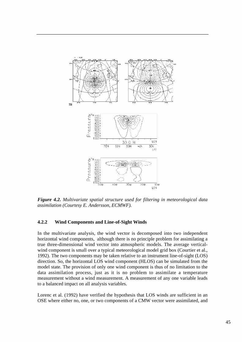
45

Figure 4.2. Multivariate spatial structure used for filtering in meteorological dataassimilation (Courtesy E. Andersson, ECMWF).

4.2.2 Wind Components and Line-of-Sight Winds

In the multivariate analysis, the wind vector is decomposed into two independenthorizontal wind components, although there is no principle problem for assimilating atrue three-dimensional wind vector into atmospheric models. The average vertical-wind component is small over a typical meteorological model grid box (Courtier et al.,1992). The two components may be taken relative to an instrument line-of-sight (LOS)direction. So, the horizontal LOS wind component (HLOS) can be simulated from themodel state. The provision of only one wind component is thus of no limitation to thedata assimilation process, just as it is no problem to assimilate a temperaturemeasurement without a wind measurement. A measurement of any one variable leadsto a balanced impact on all analysis variables.

Lorenc et al. (1992) have verified the hypothesis that LOS winds are sufficient in anOSE where either no, one, or two components of a CMW vector were assimilated, and

they found half the impact when only one wind component, rather than both, wasused. Moreover, in an additional experiment, where 50% of all CMW vectors wererandomly removed, 50% of the impact of all CMW was also found. Thus, the expectedanalysis impact of two-wind-component measurements is the same for two collocatedorthogonal components and for two spatially well-separated measurements of onesingle component. This means that matching of multiple azimuth ‘looks’ in onegeographical area is not very useful.

At very small scales (e.g. the footprint of a DWL) and in extreme cases (e.g.thunderstorms) the vertical component of the wind may be quite substantial and theassumption to neglect vertical motion is strictly not valid in such situations. However,current NWP models cannot represent these small scales and as such the verticalmotion is regarded as an unwanted component of the measurement and treated as partof the so-called representativeness error. The representativeness error is furtherdiscussed below.

4.3 Coverage Requirements

4.3.1 Vertical Domain

While observations of wind profiles are most wanted in the upper troposphere, i.e.between 5 and 16 km (upper limit depending on latitude) wind profiles will be usefulover the full range between 0 and 16 km. In addition, as more forecast models arebeing extended into the stratosphere, wind profiles in the lower stratosphere (between16 and 20 km) will be useful as well.

4.3.2 Vertical Resolution

In the vertical, meteorological model levels are at roughly 500-1000 m separation andtypical error correlation lengths around 2000 m. Range integration over 1000 m is thusappropriate. The required resolution in the stratosphere is lower, i.e. 2000 m. In theplanetary boundary layer the required useful resolution is higher because of theparticular vertical structure of the flow. On the other hand, observations close tosurface are relatively abundant in the current GOS (e.g. scatterometer, SSM/I windsand CMW) so new wind observations are expected to have less impact than those inthe higher troposphere.

4.3.3 Horizontal Domain

Wind-profile observations are required globally. Due to the shortcomings of thecurrent observing system (see Section 2.2), they are particularly needed over theoceans, in the tropics, and in the Southern Hemisphere.

47

4.3.4 Horizontal Resolution

What horizontal scales are resolved in current meteorological analyses depends on thecurrent GOS and on the data-assimilation methodology. Although both meteorologicalmodels and analysis methodologies are evolving, it is noted that the spatial extent ofthe horizontal error correlation structures (such as in Fig. 4.2) is to some extentdetermined by the density of the GOS. If a much denser observation network wasavailable, then smaller scales would be resolved. However, it is difficult to achievethis with a single supplementary observation type, so it is not expected that the spatialextent of these functions will change dramatically in the coming decade, without theavailability of a global wind-profiling network (see also Section 2.4).

Small-scale weather is determined by coherent structures such as that provided by thestructure functions (see Fig. 4.2). Currently, the transverse wind correlation distance isroughly 200 km (half-width half-maximum). This means that one observation mainlyprovides information on the error of the model state in a spatial context of about200 km. Consequently, observation information on the model atmospheric state isindependent as long as observations are at least separated by 200 km. Reflecting theabove needs, a horizontal sampling of 200 km is required for the ADM.

There is no requirement on a particular sampling scheme since the assimilationprocess is capable of handling varying spatial representation.

4.3.5 Space and Time Scales

A requirement on temporal coverage may be derived by considering the typical timescale of evolution associated with structures of a spatial dimension equal to thestructure functions. This time scale is a day, and a sensible requirement is full globalsampling every 12 hours.

If each wind profile represents a box of 200 km by 200 km on the Earth’s surface, thenthe total Earth surface contains about 13 000 boxes. Therefore, 26 000 independentwind-component-profile observations every 12 hours would define the three-dimensional global wind vector field completely, resulting in about 2000 observationsper hour. It is clear that the threshold coverage, which beneficially impacts theanalyses and can be used to demonstrate the potential of a spaceborne wind-profilingmission, can be significantly smaller. This is reflected in Table 4.1 (and the results inSection 2.3), which indicates the potential for improving meteorological analyses bywind profiling. It is useful for future operational missions to have capabilities beyondthat of the ADM.

An improved analysis of the atmospheric flow will lead to an mproved NWP skill.Experiments (OSE) with conventional radiosonde wind profiles at ECMWF (Kelly,1997, and Ingmann et al., 1999) and NCEP (Atlas, 1998) have shown that the densityof this network is sufficient to be a key component of the GOS for providing NWPimprovement (see Section 2.3). However, its coverage is limited to land areas andfurthermore most concentrated over Europe and the USA; the total number of windcomponent profiles is 1200 per 12 hours (600 vector profiles) or 100 per hour. Basedon these findings emerging from the OSEs, it is argued that the extension of the wind-profile coverage to the oceans at a similar density to the current (land-based)radiosonde network would provide an analysis with much more uniform quality. Thiswould improve atmospheric flow analyses and be of great benefit to NWP and climatestudies. Therefore, 100 HLOS profiles are required for the ADM.

4.4 Quality of Observations

The quality of observations can be expressed in terms of their accuracy, errorcorrelation and reliability.

4.4.1 Definitions

For wind observation in low-backscatter regime, the number of events (photoelectons)per measurement interval, detected at receiver level, can be close to the number of‘noise’ events. Speed estimation performed on such noisy signal leads to bad estimatesof speed for some realisations of the process where noise mimics the signal. Makingmany realisations of the process with a given retrieval algorithm, a probability densityfunction (PDF) of the speed estimation (VW) can be computed. It looks like a cluster oflocalised good estimates (bell shape) around the true mean speed (Vtrue) sitting on apedestal of uniformly distributed bad estimates (shaded zone) extending over the windsearch window (2.Vsearch), as shown in Figure 4.3.

An approximate model of the estimation PDF is as follows:

−−+−=

2

2

2

1 2

)(exp

)2(

1)1()(

W

trueW

Wsearch

W

VVFV

FVPDFσσπ

(4.1)

The accuracy (σW) is the random part of the wind-speed estimation error. It is definedas the standard deviation of the estimates (σW) (good estimates) falling under the bellshape. The reliability (F) is the complement to unity of the percentage of estimates(bad estimates) contained in the pedestal of uniform distribution.

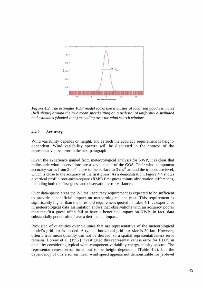
49

Figure 4.3. The estimates PDF model looks like a cluster of localised good estimates(bell shape) around the true mean speed sitting on a pedestal of uniformly distributedbad estimates (shaded zone) extending over the wind search window.

4.4.2 Accuracy

Wind variability depends on height, and as such the accuracy requirement is height-dependent. Wind variability spectra will be discussed in the context of therepresentativeness error in the next paragraph.

Given the experience gained from meteorological analysis for NWP, it is clear thatradiosonde wind observations are a key element of the GOS. Their wind componentaccuracy varies from 2 ms-1 close to the surface to 3 ms-1 around the tropopause level,which is close to the accuracy of the first guess. As a demonstration, Figure 4.4 showsa vertical profile root-mean-square (RMS) first guess minus observation differences,including both the first-guess and observation-error variances.

Over data-sparse areas the 2-3 ms-1 accuracy requirement is expected to be sufficientto provide a beneficial impact on meteorological analyses. This requirement issignificantly higher than the threshold requirement quoted in Table 4.1, as experiencein meteorological data assimilation shows that observations with an accuracy poorerthan the first guess often fail to have a beneficial impact on NWP. In fact, datasubstantially poorer often have a detrimental impact.

Provision of quantities over volumes that are representative of the meteorologicalmodel’s grid box is needed. A typical horizontal grid box size is 50 km. However,often a true mean quantity can not be derived, so a spatial representativeness errorremains. Lorenc et al. (1992) investigated this representativeness error for HLOS indetail by considering typical wind-component-variability energy-density spectra. Therepresentativeness error turns out to be height-dependent (Table 4.2), but thedependency of this error on mean wind speed appears not demonstrable for jet-level

winds (at 10 km height). This error should be added to the detection and processingerrors (error variances) of a wind-profile measurement before attempting to validate itagainst the accuracy requirement. A line-averaged wind has a smallerrepresentativeness error than a point measurement by a factor of √2. For the ADM, ahorizontal integration of 50 km within a 200 km box (see Section 4.3) is required.

Figure 4.4. Vertical profile RMS first guess minus observation differences –differences (left) and biases (right) in ms-1 for Northern Hemisphere latitudes between20 and 90 degrees. The vertical axis is in hPa (left). Dashed lines indicate thedifferences of the radiosondes with the analysis. The graphs provide an indication ofthe first guess and radiosonde wind errors (Courtesy L. Isaksen, ECMWF).

Pressure [hPa] Point Error [ms-1] Line Error [ms-1]1000 2.1 1.5750 2.0 1.4500 2.4 1.7250 3.3 2.3150 2.4 1.750 2.1 1.5

Table 4.2. Spatial representativeness error for a point measurement and for aline–averaged component wind for a 50 km horizontal scale.

Observation accuracy and first-guess-field accuracy are used to determine the weightof an observation over the first guess. Improper prior specification of the observationerror will therefore lead to a wrong assessment of the value of the observation, andconsequently to an inferior analysis. As DWL winds have variable accuracy, it isimportant to develop algorithms that are able to define their accuracy prior toassimilation.

51

From these consideration an accuracy of 2-3 ms-1 over the height range from 2 to16 km is required from the ADM.

4.4.3 Error Correlation

Bias has a context-sensitive interpretation and as such this term may cause confusion.Spatial or temporal error correlation is more specific if one furthermore specifies thespatial or temporal scales involved. Below, several relevant spatial scales arediscussed. Error correlation requirements on the smallest or shortest scales are usuallythe most difficult to meet.

Spatially correlated error is potentially very damaging in data assimilation, inparticular when the error structure is a priori not well known. For example, the spatialerror structure in satellite temperature and humidity profiles (TOVS) has been aproblem in meteorological data assimilation for more than a decade. In particular,when the precise spatial observation error correlation characteristics are poorly known,then the analysis may have high-pass-filter characteristics and the resulting analysiscan be noisy.

Any systematic error in the analysis will have the multivariate and spatial structureprescribed by the structure functions, i.e. the error is meteorologically balanced andwill influence the evolution of the model state in an effective way. Air-mass-dependent errors are the most damaging, since these potentially change the way inwhich air masses interact.

One piece of information required from wind profiles is the vertical wind-shear. Thefirst-guess vertical error-correlation scale is small and so, given the filter properties ofthe analysis, it is clear that any vertical correlation structure of error in the wind-profile measurements may be potentially very damaging, since the wind-shearinformation may be lost. If the aim is to be able to measure a wind shear of 2 ms-1

between two adjacent levels, then a correlated error of a few tenths of a ms-1 mayalready significantly blur the detection of such shear instability. (Note that a dataassimilation system can handle wind-shear measurements directly. However, in thiscase it is even more important to have independent measurements in a vertical windprofile.)

Correlation of error between profiles, although possibly less damaging than verticalerror correlation, does require attention. Experience with other satellite sensors hasshown that systematic errors or errors that depend only on specific instrumentcharacteristics or orbit phase (Sun angle) can be taken out by calibration against ameteorological model (e.g. Stoffelen, 1998). Obviously, in this case themeteorological model is calibrated by using conventional observations. For calibration

of an observing system against a meteorological model, it is an absolute requirementthat the observing system is stable.

In summary, a useful and practical specification for systematic offsets is that thecorrelation between the error variances of any two wind measurements is lessthan 0.01.

4.5 Reliability and Data Availability

4.5.1 Reliability

Routine data-assimilation systems include a quality-control procedure to preventmeasurements that are grossly in error affecting the atmospheric analysis. When agross error occurs, the observation does not relate to the (model) atmospheric state andcan therefore potentially damage the objective analysis, leading to an incorrect pictureof the state of the atmosphere. For conventional systems, gross errors are usually dueto transmission or instrument failure, or to unrepresentative measurements. A classicexample of the latter is the release of a radiosonde through a thunderstorm. Forecastsare known to be sensitive to gross-error elimination procedures in critical atmosphericconditions (ESA, 1996).

Many operational centres are using or developing variational analysis systems. Thevariational analysis system is quite flexible in dealing with observations with complexerror characteristics. However, for the measurements to be useful, these observationcharacteristics have to be known in detail a priori. Experience with conventionalobservation systems and associated quality control (QC) decisions in operationalmeteorological analysis indicate that the rate of gross errors presented to the analysis(after QC) should be only a few percent. As such, all signal characteristics have to beused in the processing to optimally specify the observation operator and cost functionin order to help reject measurements containing no information on the trueatmospheric state. All this is necessary to prevent random wind estimates, bycoincidence close to the true wind, from influencing the analysis. Based on thisexperience, it is required that the observations need to have a reliability of 95 %.

4.5.2 Data Availability

In a meteorological data-assimilation system those meteorological observationsprovided in a timely fashion by the GOS are compared to the first-guess atmosphericstate. As such, the error characteristics of the first guess are well monitored and thefirst guess is a well-defined reference atmospheric state. In turn, this referenceatmospheric state is used to routinely monitor and control the observations. Ifobservations are not available in due time, then this routine monitoring and control isnot performed, and special measures have to be taken to collocate the observations

53

with the meteorological model and other observations in order to characterise the errorproperties of such observations. It is clear that the routine monitoring, collocation, andcontrol of observations in the main real-time data stream is to be preferred above anoff-line processing.

After the error characteristics of a new observing system have been determined,experimentation with the assimilation of the data will commence. If the observationsare delivered in real time, then the operational data assimilation and forecast suite canbe used as a reference or for a control experiment. If it is demonstrated that the newobserving system adds to the improvement of the weather forecast of the controlexperiment, then the real-time assimilation of the data would start for NWP.

Timely data delivery is then required since analyses start at pre-specified times and adata cut-off time is applied. For NWP, acceptable data-delivery times for short- andmedium-range forecasting vary generally between 30 minutes and more than 6 hours,depending on the analysis time window and analysis cut-off delay. A data-deliveryrequirement of 3 hours is usually specified for spaceborne data (as practicable forglobal and regional NWP) and is common for polar-orbiting spaceborne operationalmeteorological instrumentation.

The length of the observational data set needed to achieve the objectives of the ADMis at least 3 years.

4.6 Conclusion

The observation requirements discussed in this chapter consider the presence of thecurrent GOS and the complementarity with it. Alike many other meteorologicalobservations, the spaceborne LOS wind-component profiles by themselves seem atfirst glance to be of limited value, but in the context of atmospheric data-assimilationsystems they would in fact be an essential component of the GOS. Besides betterweather forecasts, improved meteorological analyses are very useful for studyingcirculation and transport phenomena relevant to climate and atmospheric compositionstudies. Moreover, the meteorological analysis fields already provide consistentatmospheric data sets of wind, humidity, temperature and, in the coming years, ozoneand probably aerosol distributions. The monitoring of the quality of meteorologicalanalyses is best done in real time by collocation with and rigorous comparison to awide range of real-time meteorological observations, complemented by off-linevalidation studies.

For a mission intended to demonstrate the feasibility of a full-scale spaceborne windobserving system to improve global atmospheric analyses, the requirements on dataquality and vertical resolution are the most stringent and most important to achieve.Under this assumption, the horizontal density of observations is of the lowest priorityamongst the requirements discussed in this chapter. The derivation of the coverage

specification is supported by weather-forecast-impact experiments, which included theinputs of the conventional wind-profile network that is thin and irregular but of keyimportance. Moreover, the coverage specification reflects the WMO thresholdrequirements (see Table 4.1).

Table 4.3 provides an overview on the requirements discussed previously.

Observational Requirements

PBL Troposph. Stratosph.

Vertical Domain [km] 0-2 2-16 16-20

Vertical Resolution [km] 0.5 1.0 2.0

Horizontal Domain global

Number of Profiles [hour-1] 100

Profile Separation [km] > 200

Temporal Sampling [hour] 12

Accuracy (Component) [ms-1] 2 2-3 3

Horizontal Integration [km] 50

Error Correlation 0.01

Reliability [%] 95

Timeliness [hour] 3

Length of Observational Data Set [yr] 3

Table 4.3. Observational requirements of the Atmospheric Dynamics Mission.

As explained above, the meteorological impact in the tropics is the most certain, and,from a climate point of view, also the most useful. Moreover, to improve atmosphericanalysis beyond the tropics and in particular NWP in Europe, the above requirementshave been chosen to demonstrate the advantageous impact of DWL winds at highlatitudes.

55

The implementation of the ADM will be a major step forward in providing greaterinsight into atmospheric processes by providing wind profiles over the whole globe forthe first time. This makes this mission unique and a true explorer mission.

57

5 Mission Elements

5.1 Introduction

The innovative element of the Earth Explorer ADM is the provision of wind-component profiles by a DWL onboard a polar-orbiting satellite. The wind profileswill be provided by an instrument based on the direct detection technique. After pre-processing, the DWL data will appear as profiles of LOS winds, i.e. a profile of onewind component per observation point. These DWL data will be an extra input data setto atmospheric analysis systems, added to the other observation types currentlyavailable (see Chapter 2). The analyses provided by different data-assimilationsystems in different NWP centres will be used for climate studies, for forecasting theweather, and form the natural basis for most of the other studies. Figure 5.1 illustratesthese links.

Figure 5.1. End-to-end elements of the Atmospheric Dynamics Mission.

The direct use of LOS winds for geophysical studies will be exceptional, althoughLOS winds are likely to be used directly for validation and retrieval processdevelopment purposes. However, the backscatter data from the instrument providesinformation instrumental for some aspects of atmospheric research and will be used assuch.

5.2 Instruments and Data

5.2.1 Doppler Wind Lidar Instrument Principle

The DWL is an active instrument which fires laser pulses towards the atmosphere andmeasures the Doppler shift of the collected return signal, backscattered at different

levels in the atmosphere. The frequency shift results from the relative movement ofthe scatter elements along the line of sight of the instrument. This movement relates tothe mean wind in the observed volume. The measurement volume is determined by themaximum ground integration length of 50 km, the required height resolution and thewidth of the laser footprint. The measurements are continuously repeated at distancesof about 200 km.

Light is scattered either by interaction with aerosol or cloud particles (Mie scattering)or by interaction with air molecules (Rayleigh scattering). The two scatteringmechanisms exhibit different spectral properties and different wavelengthdependencies such that instruments evaluating only one signal type or both in separateprocessing chains can be constructed.

For Mie backscattering, the spectrum of the received Doppler shifted light equals thetransmitted spectrum slightly broadened by the wind variability within themeasurement volume. In case of molecular scattering, the Brownian motion of airmolecules significantly broadens the received spectrum to a width equivalent to windspeed such that the spectral width resembles Doppler shifts equivalent to several100 ms-1. The mean Doppler shift resulting from average air motion representstherefore in this case a much smaller fraction of the spectral width than in the case ofaerosol scattering. Thus for molecular scattering, a much higher signal is needed forthe same velocity measurement performance, but as noted above the received signallevel from molecules has different dependencies compared with aerosol scattering.

The return signal strength from aerosols scattering depends on their concentration,which varies largely over different locations, altitudes, and time. Aerosols are mostconcentrated in the lower 4 km of the troposphere and diminish above the troposphere.A system relying only on aerosol backscattering can therefore not providemeasurements at higher altitudes. On the other hand, ground return signals useful forground-speed calibration and signals from clouds exhibit the same spectral propertiesas the aerosol signal and can hence be best processed by such a receiver system.

Contrary to the Mie signal, the molecular backscattering signal under clearatmospheric conditions is only weakly dependent on the aerosol content (attenuation)and exhibits only small variation with altitude. This allows more consistentmeasurements up to altitudes above 20 km. However, Rayleigh receivers suffer fromaccuracy limitations at low altitudes (< 2 km) due to the aerosol absorption.

This complementary behaviour of Mie and Rayleigh return signals suggests acombination of two dedicated receivers in a single instrument in order to allowaccurate measurements over the entire altitude range.

There are two measurement techniques to measure these effects, namely the coherentheterodyne systems and the direct detection, interferometric systems. There are in factvery profound differences of principle in their respective operation. Coherent

59

heterodyne systems operate by beating the scattered and Doppler shifted radiation withan optical laser oscillator at the surface of a detector. The resultant electrical beat-frequency signal is thus analysed post-detection to produce the Doppler frequency. Onthe other hand, in the direct detection methods the optical signal field is analysed anddispersed in an interferometric filter prior to detection. Both systems requireinterferometric precision in the optical manipulation of the signal beam. However, dueto the very different physics of these schemes, the performances are very different inprinciple. For heterodyne systems the key parameter is shown to be the photondegeneracy – that is the number of photo-detections per optical mode (i.e. in a singlecoherence area and coherence time). In low-backscatter conditions, this requires thatthe available laser power to be distributed into pulses of the largest possible energy.However, for direct-detection interferometric systems, the accuracy depends only onthe total scattered signal and is not dependent on the energy of individual pulses, onlyon the total laser energy.

Figure 5.2. Doppler Wind Lidar principle: The lidar emits a laser pulse towards theatmosphere, then collects, samples, and retrieves the frequency of the backscatteredsignal. The received signal frequency is Doppler-shifted from the emitted laser due tothe spacecraft, Earth, and wind velocity. The lidar measures the wind projection alongthe laser line-of-sight, using a slant angle versus nadir.

There is a considerable heritage of ground and airborne laser Doppler systems forwind measurement. Validation and calibration studies have been carried out withcoherent detection of aerosol scattering at 2 and 10 µm and show performance veryclose to the expected quantum limit. Investigations include measurements throughoutthe troposphere, studies of valley drainage, boundary-layer phenomena and movementof pollution, studies of aircraft wake vortices, airborne measurements of clear-air

turbulence, wind shear and backscatter strength around the Atlantic and PacificOceans. Direct-detection systems have been developed more recently; very promisingperformance has been demonstrated with both the multi-channel (MC) and double-edged (DE) variants of the basic technique. These include scattering from both aerosoland molecular sources. All of these systems and their variants have the potential forapplication to spaceborne operation, and detailed investigations have been undertakento model their use.

5.2.2 Core Space Elements

The core space element of the ADM is ALADIN (Atmospheric Laser DopplerInstrument), a direct detection lidar incorporating a fringe-imaging receiver (analysingaerosol and cloud backscatter) and a double-edge receiver (analysing molecularbackscatter). The instrument will be accommodated on a satellite, flying in a Sun-synchronous, polar orbit, at an altitude of 400 km and with a local equator crossing at06:00 and 18:00 hrs. This orbit allows a (near-)global coverage.

The processing of the backscatter signals will produce LOS wind profiles above thickclouds or down to the surface in clear air along the satellite track, every 200 km. Windinformation in thin cloud or at the tops of thick cloud is also attainable. From the dataprocessing, information on other elements like clouds and aerosols can also beextracted. The data will be disseminated to the main NWP centres in near-real-time.

5.2.3 Ground Segment

In order to fulfil the near-real-time requirement, the proposed ground segment is basedon two receiving locations for the scientific data, situated in the Northern Hemisphere(Kiruna and the Barrows meteorological station). The downlink is based on the HRPT(high-resolution picture transmission) standard, as it is being defined and implementedfor the METOP mission, allowing the use of equipment familiar to the meteorologicalcommunity. For satellite command and control, the Kiruna Salmijaervi station will beused.

The data will then be relayed via standard communication links to the missionoperations centre. This centre takes responsibility for the spacecraft operations, as wellas the data processing up to Level 1. After the data is processed and calibrated, it willbe sent to a dedicated scientific data centre, which will be responsible for the qualitycontrol, as well as the dissemination of the data to the meteorological centres and otherend users.

61

5.3 Atmospheric Analyses and NWP Forecasts

Although any observation type can be used on its own for particular studies, it is clearthat the most powerful usage is achieved through data-assimilation systems in whichthe different data and observations are combined (synergetic use of observations andan atmospheric model) in order to provide the best estimate of the atmosphericparameters which are relevant for forecasting and other process studies. In thissynergy, the DWL measurements will complement other data in order to fill majorgaps in wind-profile observations, which currently are mainly provided by radiosondestations. No other observing system is planned to fill this gap except the ADM. TheDWL data will provide an important new input element to data-assimilation systemswhich are run in several NWP centres.

Data from other sources will be needed for the analysis of the DWL observations. Thedifferent observation types are described in Chapter 2, together with their respectiveperformances and limitations. They are in particular

• the in-situ meteorological data (surface and upper-air ground-based data) and

• the current remote-sensing data.

The link between the lidar processing and a data assimilation system will beinteractive, as it is for example already now with satellite sounder data whose retrievalis supported by the knowledge of a background field (generally a short-rangenumerical forecast, using schemes called RT-TOVS in the case of TOVS or ATOVS).A prior knowledge of the atmospheric state from a background may help the signalprocessing. It is, however, expected that the information fed back from the NWPmodels to the DWL data production will remain small, and that the lidar wind errorswill not be dependent on any NWP model error.

63

6 System Concept

6.1 From Mission to System Requirements

The mission requirements, as defined in Chapter 4, have been translated into systemobservational requirements in order to highlight the design drivers for the engineeringwork.

Measurement Accuracy Requirement

The mission requires the measurement of horizontal wind velocity components fromthe lower part of the troposphere to the lower part of the stratosphere (up to 20 kmaltitude). The observation of a single component of the horizontal wind velocity isrequired to ease the instrument design since it has been shown to be adequate for theADM (see Chapter 4). Furthermore, there is no particular requirement on the directionof the wind component to be measured.

The required instrumental accuracy for any horizontal wind component, hereaftercalled HLOS, has been translated from the mission accuracy requirement of 2-3 ms-1.The background representativeness error for a line-averaged wind componentmeasurement of 50 km (see Table 4.2) has been quadratically subtracted from themission accuracy requirement, yielding an instrumental accuracy requirement of 1-2ms-1 for the HLOS wind component. It has to be noted that this representativenesserror includes the contribution from the vertical wind component.

Stringent requirements on both wind accuracy and large vertical domain (up to 20 km)lead to consider an instrument concept relying on molecular backscatter at highaltitude, where background aerosols become rare (Vaughan et al., 1999), and onaerosol backscatter at lower altitude.

Instrument Pointing

The LOS of the instrument has to be oriented such that the HLOS measurementaccuracy is optimised. A flat optimum of HLOS measurement accuracy exists for LOSangles pointing between 35° to 50° off nadir. It results from an improvement of thehorizontally projected LOS wind accuracy, balanced by the increasing range withincreasing nadir angle. For the selected 35o LOS nadir angle, the viewing geometryrequires an instrumental LOS wind accuracy a factor 0.6 more accurate than thespecified HLOS wind accuracy, i.e. 0.6-1.2 ms-1. The lower value (0.6 m·s-1) has beenapplied for the altitude range from 0 to 2 km, whereas the higher value is consideredas a driving requirement up to the stratosphere (2 to 16 km).

Any wind-speed-component observation to be delivered to the end-users is to bereferenced to an Earth surface frame located at the vertical of the probed volume. Itimplies, at system level, an accurate knowledge of the relative velocities of thespacecraft and the local Earth frame and of the instrument LOS pointing. The spuriousDoppler shifts induced along the instrument LOS by both spacecraft and Earth rotationvelocities are typically much larger than the LOS wind speed and need to becompensated to ease the instrument design. The instrument LOS pointing is setperpendicular to the spacecraft velocity, minimising the spacecraft-velocity-inducedDoppler shift. A ‘yaw steering’ mode is implemented at spacecraft level tocompensate the HLOS Earth rotation velocity. Determination of the residual spuriousDoppler shift is performed by evaluation of ground echo signals where available. Tomaintain a sufficient knowledge of the true ground speed in periods where the groundis obscured by clouds, exact pointing measurements in combination with positionknowledge is used to interpolate between calibrations.

Spatial and Temporal Coverage

The requirement of global coverage in combination with a temporal sampling of 12hrequires a high-inclination orbit. Due to the measurement accuracy's dependency onrange, the orbit should be as low as possible, but must not impose unacceptableconstraints on the orbit (i.e. fuel needed to maintain the orbit and the requirement toensure the contact times). No particular requirement with respect to the local time ofthe wind measurements has been specified; however, measurements aroundsunrise/sunset may benefit from fewer obstructions by clouds, at least over land. Thecoverage requirement does not have an impact on the altitude. Thus, a Sun-synchronous orbit at about 400 km altitude has been chosen as an appropriatecompromise to meet the spatial/temporal coverage requirements. Furthermore, theselection of a local time at the ascending node around 6h or 18h (dawn-dusk)simplifies the layout of the solar-panel mechanics.

The integration length of 50 km and the measurement separation of 200 km imply aninstrument duty cycle of 25%.

Data Delivery Timeliness

The requirements specify a data delay not exceeding three hours. With a time for anorbital revolution of about 1.5 h, it is necessary to download measurement data onceper orbit. This requires at least two ground stations for data reception at high latitudes(e.g. Kiruna/ESA and Barrows/NOAA). Public data networks can disseminate the datadue to its small volume.

The task of the data-processing centre of the ground segment consists of derivinghigh-quality wind-component data from the raw data. This includes application of

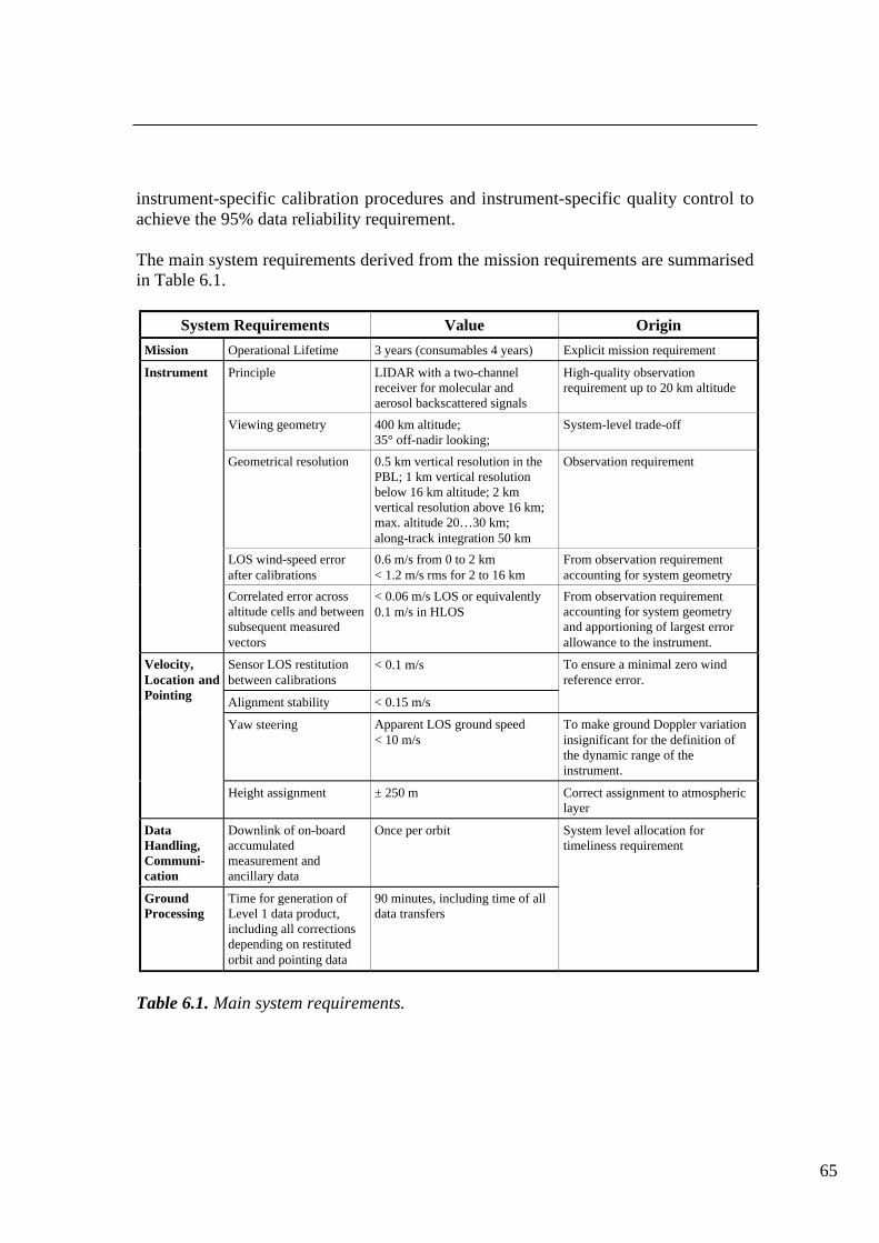
65

instrument-specific calibration procedures and instrument-specific quality control toachieve the 95% data reliability requirement.

The main system requirements derived from the mission requirements are summarisedin Table 6.1.

System Requirements Value Origin

Mission Operational Lifetime 3 years (consumables 4 years) Explicit mission requirement

Principle LIDAR with a two-channelreceiver for molecular andaerosol backscattered signals

High-quality observationrequirement up to 20 km altitude

Viewing geometry 400 km altitude;35° off-nadir looking;

System-level trade-off

Geometrical resolution 0.5 km vertical resolution in thePBL; 1 km vertical resolutionbelow 16 km altitude; 2 kmvertical resolution above 16 km;max. altitude 20…30 km;along-track integration 50 km

Observation requirement

LOS wind-speed errorafter calibrations

0.6 m/s from 0 to 2 km< 1.2 m/s rms for 2 to 16 km

From observation requirementaccounting for system geometry

Instrument

Correlated error acrossaltitude cells and betweensubsequent measuredvectors

< 0.06 m/s LOS or equivalently0.1 m/s in HLOS

From observation requirementaccounting for system geometryand apportioning of largest errorallowance to the instrument.

Sensor LOS restitutionbetween calibrations

< 0.1 m/s

Alignment stability < 0.15 m/s

To ensure a minimal zero windreference error.

Yaw steering Apparent LOS ground speed< 10 m/s

To make ground Doppler variationinsignificant for the definition ofthe dynamic range of theinstrument.

Velocity,Location andPointing

Height assignment ± 250 m Correct assignment to atmosphericlayer

DataHandling,Communi-cation

Downlink of on-boardaccumulatedmeasurement andancillary data

Once per orbit

GroundProcessing

Time for generation ofLevel 1 data product,including all correctionsdepending on restitutedorbit and pointing data

90 minutes, including time of alldata transfers

System level allocation fortimeliness requirement

Table 6.1. Main system requirements.

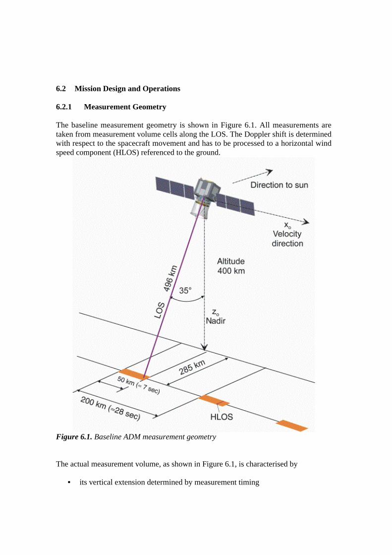
6.2 Mission Design and Operations

6.2.1 Measurement Geometry

The baseline measurement geometry is shown in Figure 6.1. All measurements aretaken from measurement volume cells along the LOS. The Doppler shift is determinedwith respect to the spacecraft movement and has to be processed to a horizontal windspeed component (HLOS) referenced to the ground.

Figure 6.1. Baseline ADM measurement geometry

The actual measurement volume, as shown in Figure 6.1, is characterised by

• its vertical extension determined by measurement timing

67

• the integration length in the flight direction determined by the number ofpulses contributing to a single Doppler evaluation, and

• a negligible extension in the direction orthogonal to both other directions.

The measurement volume of the return signal from a single shot is defined by thelateral extension of the transmitted beam (a few metres in diameter) and the timegating of the receiver, which is adopted to the desired vertical resolution (several100 m to 2 km). Furthermore, it is assured that the spatial pulse length is much shorterthan the desired vertical resolution. Due to the fact that the signal from a single shot istoo weak for the evaluation, several shots along a ground track of up to 50 km have tobe accumulated.

6.2.2 Orbit Selection

Orbit Parameters

As justified in 6.2.2, a Sun-synchronous dawn-dusk orbit has been selected. Itprovides quasi-global coverage (the 7° polar gap is acceptable) and corresponds to alower cloud coverage. Moreover, it facilitates some aspects of the satellite design.

The LOS of the instrument will be 35° off nadir to ensure the best instrumentperformance, and 90° across the flight direction to avoid a contribution from thesatellite velocity to the Doppler-frequency shift. As the instrument should not pointtoward the Sun, the LOS of the instrument will point to the anti-Sun direction. Theselected dawn-dusk orbit will have a LTAN of 18:00 in order to provide a slightlybetter coverage over the North Pole. The resulting orbit geometry and the instrumentorientation is depicted in Figure 6.1.

There have been no specific requirements driving the choice of the orbit altitude. Theresulting freedom has been used to optimise the mission performance while reducingthe satellite and ground-segment complexity. Detailed performance simulations havebeen done, taking into account the main instrument parameters (telescope diameter,laser power and PRF) and the main system parameters (fuel demand and frequency oforbit maintenance manoeuvres), as well as the number of ground stations required.Orbits between 350 km and 450 km altitude are best suited in order to optimise theoverall system (Fig. 6.2).

A baseline altitude of 400 km has been selected. Its parameters are summarised inTable 6.2. This orbit represents a compromise between instrument performance, datadown-link capability and orbit maintenance requirements, because it offers at least onedata down-link per orbit assuming only two ground stations, and reduces the fueldemand to about 65 kg for the required mission lifetime.

Figure 6.2. Orbit altitude versus instrument performance and fuel consumption.

Mean Orbit Parameters

Orbit Type Sun-synchronous frozen orbitat 18:00 LTAN

Altitude at Ascending Node 400 km

Mean Altitude 408 km

Reference Epoch 21.3.2004, 12:00:00

Semi-Major Axis 6769.14 km

Eccentricity 0.001165

Inclination 96.99°

RAAN 90°

Argument of Perigee 90°

True Anomaly -90°

Table 6.2. Parameters of selected baseline orbit.

The selected orbit corresponds to a frozen orbit, offering constant instrument rangegate timing parameters for each specific latitude. In this case the radial velocity of thespacecraft, i.e. the radius rate, is only a function of the latitude, which simplifies the

69

yaw steering control law. Figure 6.3 shows the altitude and altitude rate of the satellitedue to the reference Earth ellipsoid (WGS ‘84) and the orbit eccentricity.

Figure 6.3. Altitude and altitude rate of selected 400 km orbit.

Orbit Maintenance

The estimated altitude decay rates are depicted in Figure 6.4, for an effective cross-sectional area of the satellite of 3 m2, corresponding to the selected baseline satelliteconfiguration described in Section 6.4. For the 400 km orbit, the altitude decay after

Figure 6.4. Orbital decay and fuel consumption.

30, 60 and 90 days is rather moderate and periods of up to 90 days are feasible withoutany orbit manoeuvre. Over the required mission lifetime of 3 years plus 1 year forconsumables, the fuel consumption for maintaining the baseline altitude of 400 kmwill be about of 54 kg of hydrazine.

Ground Station Visibility

The ADM data shall be delivered to the user within 3 hours after data acquisition. It isnecessary to have ground station contacts every orbit. A two-station combination hasbeen selected. These are the existing ESA ground station in Kiruna and a second onein Barrow, a meteorological station located in the northern part of Alaska. Theresulting ground-station visibility, assuming a minimum elevation angle of 5°, isdepicted in Figure 6.39. The Barrow station already offers meteorological services andprovides sufficient infrastructure for ground-station maintenance. The TC/TM groundreceiving station will be co-located with the data receiving station in Kiruna.

6.2.3 Measurement Profile

Due to the required profile separation, the instrument will be operated with a dutycycle of 25 %. It will be fired during 6.93 seconds (equivalent to 50 km ground track)followed by a gap in observations of 20.79 seconds (equivalent to 150 km). Asdetailed later, the horizontal accumulation length can be varied from 500 m (Mie orRayleigh channel) to 50 km without affecting performance for the integration over thefull 50 km. The vertical sampling profile includes some altitude margin in order toensure that the ground echo is acquired when the ground is visible, in order to providecalibration data.

All vertical integration intervals are pre-programmable with a vertical resolution,selectable between 100 m and 2 km up to an altitude of 40 km. The baselinemeasurement profile is depicted in Figure 6.5.

71

Figure 6.5. The baseline measurement profile, depicting the mapping of atmosphericheights to layers measured by the detector. The vertical as well as the horizontalvalues can be programmed, thus providing good flexibility.

6.2.4 Solar-Array Arrangement

Figure 6.6 depicts the relative orientation of the orbit plane with respect to the eclipticplane for the summer and the winter solstice, while Figure 6.7 shows the eclipse timesfor the first year of the mission (2004). The angle between the orbit plane and theecliptic is 60° during the summer solstice and 74° during the winter solstice. Themaximum eclipse time during the summer solstice is about 27% of the orbit period.The solar array will be tilted about 10° relative to the orbital plane to optimise theenergy generation during the phase with eclipse. This angle corresponds to a meanloss of efficiency of approx. 12% during non-eclipse times.

Figure 6.6. Orbit orientation during summer and winter solstice.

Figure 6.7. Eclipse duration for the 400 km orbit.

6.2.5 Mission Operation and Phases

The ADM is divided into distinct phases, namely the pre-launch and the launch andearly orbit phase (LEOP), followed by the commissioning phase for the satellite aswell as the instrument. This is followed by the normal operations phase of the mission.The launch phase and LEOP are described with the launcher in Section 6.5.

73

Commissioning Phase

After a successful LEOP, the satellite is in a safe hold mode. In this state, it can stayunattended for several days without any operation. From that moment on, thecommissioning phase will begin. The main components of the satellite will bevalidated and the attitude will be changed into geocentric pointing. In a next step theyaw steering will be activated and a first thermal and electrical checkout of theinstrument components will be performed. Then the instrument can be switched-onand first functional and performance tests can be established. After a thoroughvalidation of all functions, normal operations can be started.

Normal Operation

During normal operation, the spacecraft will be operated in the yaw steering mode andthe instrument will perform measurements over the complete orbit. The spacecraftwill be capable of operating autonomously for at least 72 hours. As part of theinstrument calibration, the receiver will be calibrated once per orbit for a period of5 minutes. This calibration period can be performed over areas of less scientificinterest, e.g. the poles. Orbit manoeuvres will be performed once per month.

6.3 The ALADIN Instrument

6.3.1 Instrument Concept Selection

Numerous instrument options have been investigated during the Phase-A (see Fig.6.8), ranging from coherent lidars at 9-10 µm, 2 µm and 1.5 µm to direct detectionlidars at 1.5 µm, 1 µm, 0.53 µm and 0.35 µm. Detailed performance analyses andtechnology reviews have been performed for all these concepts. All coherent conceptsuse aerosol (Mie) scattering and have similar performance behaviour, providing highaccuracy at low altitude and reduced reliability above a given altitude threshold,depending on the aerosol conditions and the emitted laser energy.

Coherent Concepts

The coherent concept at 1.5 µm was rejected because of the low transmitter maturityand efficiency. The coherent concept at 9-10 µm was investigated in more detail, buthas finally been put aside, mainly because of the difficulty of developing a space-qualified CO2 laser, coupled with low industrial interest. The 2 µm system was furtherstudied as it represented the best compromise in terms of performance and technicalmaturity among the coherent concepts.

Figure 6.8. Instrument concepts studied in the trade-off activities during the Phase-A.

Incoherent Concepts

The direct detection at 1.5 µm was disregarded due to the poor maturity status of laserdevelopment. The 1 µm and 0.53 µm concepts were rejected because of lowperformance due to power limitations (for eye-safety reasons). The direct detectionultraviolet (UV) concept at 355 nm has been investigated in aerosol (Mie) andmolecular (Rayleigh) measurement modes and a combination of both was selected asthe best compromise in terms of performance, especially for its robustness vis-à-visthe aerosol-content variations.

Two concepts (2 µm coherent and 0.35 µm incoherent) have been further investigatedin detail and compared with regard to performance, technical maturity, programmatics,and growth potential for a future operational mission. The coherent lidar at 2 µmfeatures high accuracy at low altitude, but is limited to medium altitudes. Thisrestriction comes mainly from the limited potential for a significant increase in laserpulse energy for such a system. The opto-mechanical and thermal concept was alsoconsidered rather complex (due to the laser crystal cooling and alignmentrequirements), and the programmatic risk was considered relatively high because onlya single and non-European procurement source for the transmitter could be identified.Finally, the growth potential of the concept for a future operational mission is limited,since the aerosol concentration is quite low at higher altitudes.

75

Thus, the direct-detection UV concept has been selected as the baseline for ADM as itprovides good performances up to high altitudes, and has high potential for anoperational mission. A combined aerosol (Mie channel) and molecular (Rayleighchannel) receiver has been defined, in order to benefit from their complementarity.This concept can provide compliant wind measurements up to high altitudes (20 kmand above) for an operational mission, basically independent of the aerosol content.The technical and programmatic risks were evaluated as low, as transmitter andreceiver units with similar or better performances have already been developed and asmultiple and European supplier sources are identified for each critical element.Finally, the growth potential for the future operational mission is sufficiently high thata mission fully compliant with the ideal WMO requirements can be proposed, basedon the ADM instrument concept.

6.3.2 Technical Details of the selected Baseline

Operating Principle

The spaceborne lidar will emit a narrow linewidth laser pulse (a few tens of MHz) atan ultraviolet wavelength (355 nm). The laserbeam will be sent towards theatmosphere in a slant angle at 35° (Fig. 6.1). The laser light will then be scattered byaerosol particles (Mie lidar) and molecules (Rayleigh lidar) and a small partbackscattered towards the lidar. The received signal frequency is Doppler-shiftedrelative to the emitted laser due to spacecraft movement, the Earth’s rotation, and thewind velocity along the line-of-sight. In the proposed ADM concept, the spacecraftand Earth’s rotation Doppler shifts are minimised by the use of a proper satelliteattitude-control scheme (yaw steering mode). The instrument thus directly measuresDoppler wind shifts, which can be expressed as follows:

fV ∆= .2

λ (6.1)

where V (m/s) is the wind velocity along the line-of-sight, λ is the wavelength, and ∆fis the frequency Doppler shift.

Winds are measured in clear air (i.e. above or in the absence of thick clouds), andwithin and through thin clouds (e.g. cirrus). The laser pulse is emitted at a relativelyhigh repetition rate (100 Hz) such that subsequent laser shots can be averaged in orderto reduce detection noise. Due to the satellite’s movement, these laser shots form aline on the ground. The integration length is limited to 50 km in order to be compatiblewith the mission requirements.

The received light is collected by a telescope and is directed onto a receiversubsystem. The receiver samples the signal in the time domain in order to determineits arrival time and hence the distance to the atmospheric layer. For each layer the

spectral distribution of the return signal is analysed through a high-resolutionspectrometer. Direct detection is used to measure the spectrum, requiring low-noise(quasi photon-counting) detectors which are available for the selected ultravioletwavelength.

The return signal spectrum in Figure 6.9, is the sum of a wide-bandwidth Rayleighsignal due to molecular scattering (equivalent to 600 m/s FWHM) and a narrow-bandwidth Mie signal due to aerosol scattering, whose bandwidth is set by the laserspectrum (10 m/s FWHM typically).

Various techniques are available to measure the Rayleigh and Mie spectrum centralfrequency and they fall into two categories: fringe-imaging and edge techniques. Anextensive trade-off has been performed between these two options during Phase-A,both in terms of performance and technical implementation.

Figure 6.9. Spectral properties of the scattered return signal: The narrow bandwidthaerosol (Mie) signal is superimposed with the broadband molecular (Rayleigh) signal.

The fringe imaging technique (see Fig. 6.10) will be used for the Mie receiver. Thisconcept was preferred over the edge technique as the latter is too sensitive to theRayleigh background in the ultraviolet. It is intended to sample the received spectrumwith a resolution compatible with the spectrum width. A centroïd computation thenprovides the location of the spectrum centre. The fringe width obtained is set by thelaser spectrum and the spectrometer resolution. After multi-channel sampling, thefringe spreads over a few spectral intervals. The total number of intervals is defined bythe useful range (wind dynamic range + margin) of the receiver. The fringe issuperimposed on the Rayleigh and atmosphere radiance spectra, which provideadditional noise. This noise is kept negligible by making use of blocking spectralfilters.

77

Figure 6.10. Mie receiver principle: multi-channel spectrometer with fringe imagingTop: Spectrometer illumination; Bottom: Measured spectrum.

The edge technique (Fig. 6.11) is used for the Rayleigh receiver. This concept waspreferred over the fringe imaging technique which features similar performance butwhose implementation imposes tighter alignment and detector requirements. Twofilters are placed symmetrically from the centre wavelength position in order toperform a differential measurement. The filter outputs (A and B) are used directly asthe estimator for the frequency shift.

The receiver concept proposed for ADM is capable of using both measurementprinciples simultaneously. A spectral filter extracts the central part of the spectrum anddirects it towards the Mie receiver, whereas the wings of the spectrum are routed tothe Rayleigh receiver.

Figure 6.11. Rayleigh receiver principle: Edge measurement with two filters.

Instrument Overall Architecture

The baseline lidar instrument is based on a 130 mJ (150 mJ design goal) / 100 Hzdiode-pumped frequency tripled Nd:YAG laser, and a 1.1 m diameter telescope. Thepower laser head is composed of a medium power oscillator, an amplifier, and atripler. A small reference and seed laser head is used as frequency reference and isinjected into the resonator through fibre optics. Two of each of the laser heads will beimplemented for redundancy. The power laser head is conductively cooled via heatpipes, which are attached to the main heat sources, namely the laser slabs and thepump diodes. The heat pipes transport the heat flux to dedicated radiators on the anti-Sun side of the spacecraft. The laser head is derived from past developments inEurope.

In order to provide optimum performance over the whole altitude range, a combinedMie and Rayleigh receiver will be implemented. The Mie receiver is composed of aFizeau spectrometer, associated to a thinned back-illuminated UV Si-CCD detectorworking in an accumulation mode which allows photon counting. This spectrometerhas been validated in the frame of the ESA Technology Research Programme. TheRayleigh receiver is a double Fabry-Perot etalon, which analyses the wings of theRayleigh spectrum with one CCD and two read-outs. This technique has beenvalidated on ground by several laboratories, though with photomultiplier detectors(Garnier and Chanin, 1992; Chanin et al., 1994; Rees et al., 1996; Flesia and Korb,1999). The CCD provides significantly higher quantum efficiency, and hence aperformance gain.

A Cassegrain afocal telescope is used for both emission and reception. An isothermaland lightweight design based on an advanced material like SiC or C/SiC is proposed

79

for the telescope mirrors and structure, yielding the required optical quality andstability without a focusing or alignment mechanism.

The direct-detection receiver principle allows one to obtain an overall opto-mechanical design with large margins for the optical quality and pointing-stabilityperformance. The proposed method for the emission / reception switch is apolarisation beam splitter associated to quarter-waveplate, which has been validated inthe clear atmosphere by ground-based lidars.

The instrument core, which consists of the opto-mechanical part, the receiver and thedetectors (Fig. 6.12 and Fig. 6.13), will be mounted on the top face of the spacecraftvia three bipods. The instrument electronics (detection, transmitter) are mounted onthe internal side of this top face. These electronics are connected to a radiator locatedon the anti-Sun side. The instrument core will be protected by a thermal bafflemounted on the satellite panel.

The star trackers (one operating, one cold redundant) are used for attitude estimation,which is used for control as well as the Doppler retrieval when no ground echo isavailable. They will be mounted on the instrument structure in order to limitmisalignment errors.

Figure 6.12 Layout of the instrument core, consisting of the opto-mechanical part,the receivers and the transmitters.

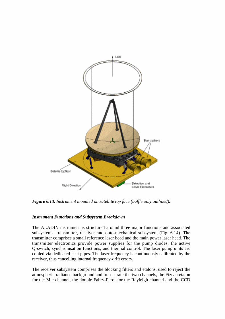
Figure 6.13. Instrument mounted on satellite top face (baffle only outlined).

Instrument Functions and Subsystem Breakdown

The ALADIN instrument is structured around three major functions and associatedsubsystems: transmitter, receiver and opto-mechanical subsystem (Fig. 6.14). Thetransmitter comprises a small reference laser head and the main power laser head. Thetransmitter electronics provide power supplies for the pump diodes, the activeQ-switch, synchronisation functions, and thermal control. The laser pump units arecooled via dedicated heat pipes. The laser frequency is continuously calibrated by thereceiver, thus cancelling internal frequency-drift errors.

The receiver subsystem comprises the blocking filters and etalons, used to reject theatmospheric radiance background and to separate the two channels, the Fizeau etalonfor the Mie channel, the double Fabry-Perot for the Rayleigh channel and the CCD

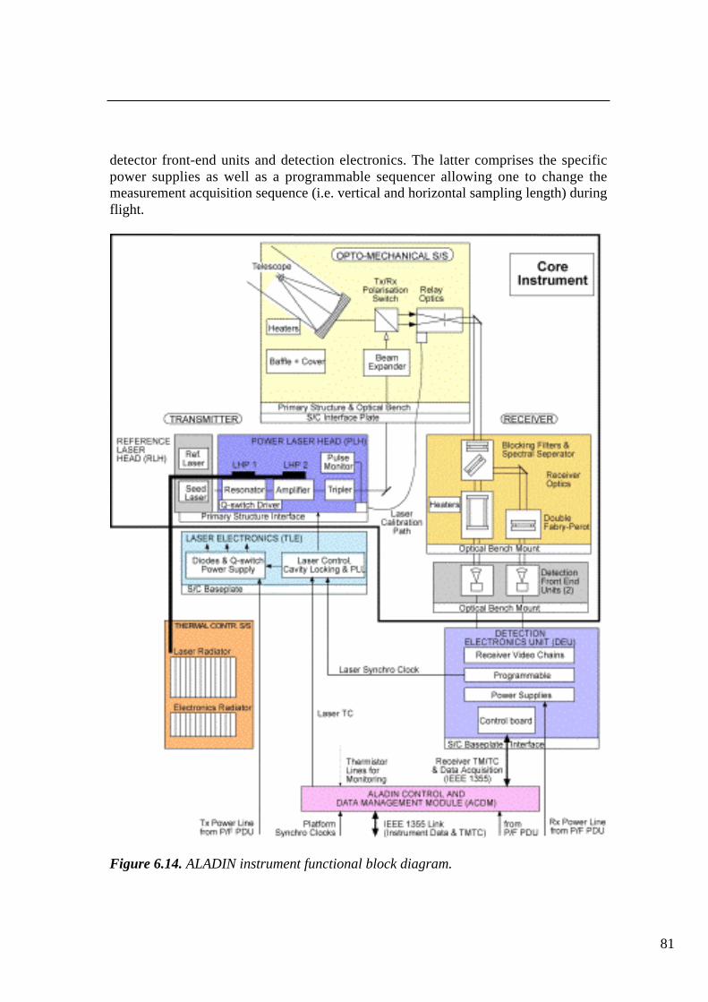
81

detector front-end units and detection electronics. The latter comprises the specificpower supplies as well as a programmable sequencer allowing one to change themeasurement acquisition sequence (i.e. vertical and horizontal sampling length) duringflight.

Figure 6.14. ALADIN instrument functional block diagram.

The opto-mechanical subsystem includes the telescope as well as ancillary optics forthe laser (beam expander) and for the received path (relay optics) in order to matchthese beams to the telescope. The polarisation switches between the telescope are alsopart of this package and implemented on the optical bench.The main characteristics ofthe instrument are summarised in Table 6.3.

Parameters Value

PlatformAltitudeOrbitNadir slant angle

400 kmSun-synchronous 6 h – 18 h

35°Transmitter

WavelengthPulse energyRepetition rateLine widthDuty cycle

355 nm130 mJ (150 mJ goal)

100 Hz30 MHz

25%Receiver

Fizeau line width (Mie)Double Fabry-Perot (Rayleigh)

Line widthSpacing

Optical efficiency (Mie/Rayleigh)Detector quantum efficiency(Mie/Rayleigh)

30 MHz

2 GHz5 GHz

3.1% / 4.6%75%

Signal ProcessingAltitude range (Mie + Rayleigh)Vertical resolutionOn-chip horizontal accumulation lengthProcessing integration length

-1 to +26.5 km (extendable)1 km (adjustable)

3.5 km (adjustable)50 km

Opto-mechanical SubsystemTelescope diameterOptical efficiency

1.1 m0.8

Table 6.3. Major instrument characteristics.

The overall instrument-control and data-management functions are included in aspecific software module, which is implemented as a module of the central data-handling subsystem in order to optimise the interface budgets and development cost.This module controls the transmitter and receiver electronics and interfaces with thesatellite data bus.

83

The transmitter laser heads, electronics and thermal-control system and the receiverand control electronics are appropriately redundant.

Transmitter

The selected configuration is a diode-pumped Nd:YAG laser with a medium-poweroscillator and single amplifier. The oscillator is actively Q-switched by a Pockels cell.To achieve a single frequency mode, the injection seeding technique is used with alow-power continuous-wave (CW) single-frequency laser. The medium oscillatoroutput energy is about 100 mJ and is amplified by a single amplifier yielding 350 mJat 1064 nm. The second and third harmonic generation crystals are placed external tothe cavity, behind the amplifier. After frequency tripling, the laser produces about130 mJ in the ultraviolet (355 nm). The key parameters are summarised in Table 6.4.

Parameter ValueType Diode-pumped Nd:YAG

Active Q-switchEmission wavelength 355 nmPulse energy 130-150 mJPulse repetition rate 100 HzPulse width 15 nsSpatial mode unique, TEM00Longitudinal mode uniqueSpectral width (FWHM) < 30 MHzBeam quality M2<2Electro-optical efficiency 2.5%

Table 6.4. Major laser characteristics.

The laser electrical efficiency is about 2.5% and the power consumption in emittingmode is 450 W. The laser is operating at about 25% duty cycle, as required for themeasurement, resulting in an average power consumption of 110 W. At minimum,twelve laser diodes with 1 kW peak power, 150 µs duration are used for each pumpunit (oscillator, amplifier). The typical lifetime of these diodes is about 5⋅109 shots,whereas the ADM requires at most 109 shots.

The oscillator design is based on an existing diode-pumped Nd:YAG, injection-seeded, conductively-cooled, 100 mJ laser (Fig. 6.15). The amplifier pump unit designis based on a 300 mJ diode-pumped Nd:YAG, conductively-cooled laser. Both lasersare packaged in small volumes. For an operational mission, the design can be scaledup to yield 300 mJ in the ultraviolet, by adding two identical amplifiers.

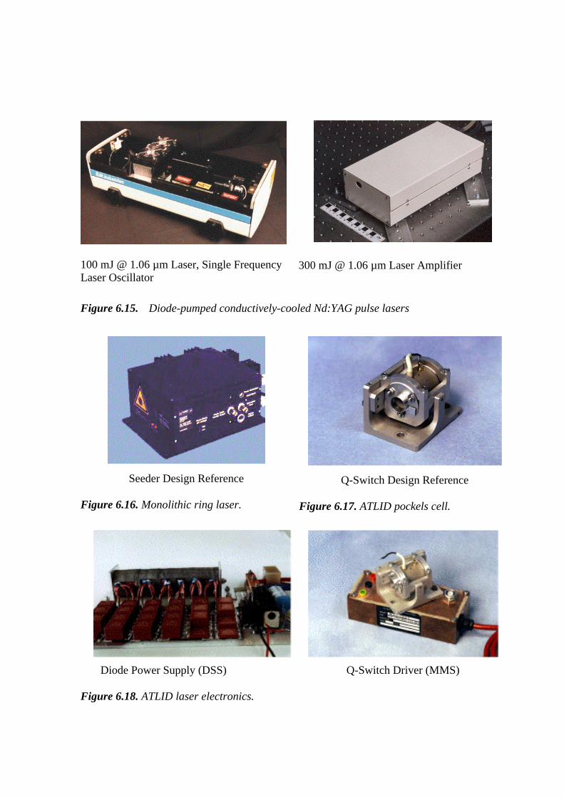
100 mJ @ 1.06 µm Laser, Single FrequencyLaser Oscillator

300 mJ @ 1.06 µm Laser Amplifier

Figure 6.15. Diode-pumped conductively-cooled Nd:YAG pulse lasers

Seeder Design Reference

Figure 6.16. Monolithic ring laser.

Q-Switch Design Reference

Figure 6.17. ATLID pockels cell.

Diode Power Supply (DSS) Q-Switch Driver (MMS)

Figure 6.18. ATLID laser electronics.

85

The ATLID Q-switch breadboard design, (Fig. 6.17), has been successfully submittedto performance and vibration tests. It will be re-used in the oscillator.

The reference laser head is composed of two small non-planar Nd:YAG ring lasersfrequency-locked by means of a phase-lock loop (PLL). One laser head is accuratelytemperature stabilised (a few mK), while the other is used as injection seeder. Duringmeasurements, the frequency is stabilised within a small portion of the receiverbandwidth by stabilising the seeder temperature. During receiver response calibration,the seeder frequency is shifted from the reference laser by a known offset in the rangeof 6 GHz, using the PLL. The ring laser design is based on commercially availablecomponents providing the required performances, with margins (Fig. 6.16).

The design of the laser power supplies is based on the ATLID laser-diode power-supply breadboard (Pulse Forming Network), and on the ATLID Q-switch power-supply breadboard (MOSFET switch) (see Fig. 6.18). These two breadboards are fullyrepresentative in terms of electrical design and have been successfully submitted toperformance, thermal and EMC tests.

Receiver

The Mie channel is based on a Fizeau interferometer, made of two plates separated bya Zerodur spacer. A tilt of 4.3 µrad is introduced between the plates to provide a linearspectral dispersion. In the Mie receiver, the received laser signal produces a linearfringe whose position is directly linked to the wind velocity. The resolution of theFizeau interferometer is 100 MHz (equivalent to 18 m/s). The wind value isdetermined by the fringe centroïd position to better than a tenth of the resolution, astested by Monte-Carlo simulation.

The Rayleigh channel is based on a double Fabry-Perot etalon with a 2 GHz resolutionand 5 GHz spacing. The etalon is split in two zones, which are imaged separately onthe detector. The wind velocity is proportional to the relative flux difference betweenthe two etalons.

Both types of filters have actually been realised and their optical performances andthermal stability have been verified (Fig. 6.22).

Interference filters and a low-resolution etalon provide a first blocking of backgroundradiation for both Mie and Rayleigh channels. The resulting equivalent bandwidth fortransmission of Earth radiance is about 240 GHz. An additional medium-resolutionetalon with a FWHM of 2.4 GHz, further reduces the equivalent bandwidth to 30 GHzin the Mie receiver.

The medium-resolution filter is also used for spectral separation of the two channels.The linear polarisation of the beam from the telescope is transformed into a circularpolarisation by a quarter-wave plate. The central part of the spectrum, containing theMie return line, is transmitted through the medium-resolution etalon while the wingsare reflected with an opposite polarisation. Upon transmission through the λ/4 plate,the reflected beam assumes a linear polarisation, perpendicular to the incomingpolarisation, which allows its separation and routing to the Rayleigh receiver.

Figure 6.19. Mie receiver principle: Fizeau interferometer and CCD detector.

Fizeau (Mie Channel) Double Fabry-Perot (Rayleigh Channel)

Figure 6.20. High resolution filters.

Two identical detector modules are implemented for the Mie and the Rayleighchannels. This significantly simplifies the development approach for the detection

87

assembly. The detector baseline is an accumulation CCD (Fig. 6.23), which allowsone to accumulate laser shots on the chip while retaining the altitude information.Because of the small number of read-outs, this technique allows the use of a thinned,back-side-illuminated Si-CCD with a high quantum efficiency in a quasi-photoncounting mode. The detector is moderately cooled (-30° C) by a Peltier element tolimit the dark current noise. Only the read-out mode differs for the Mie and Rayleighchannels, providing respectively sixteen and two outputs.

Two analogue chains are used for each channel, one measuring the atmospheric windprofile and ground echo and the second one for laser calibration. The CCD sequencingis programmable, allowing in-flight modification of the vertical and horizontalresolution of the wind measurements, giving flexibility in the partition betweenanalogue on-chip accumulation and numerical integration.

The Mie receiver can be taken as an example to illustrate the operation of theaccumulation CDD. The linear fringes are imaged in the image zone (Fig. 6.23). Afterintegration over a time corresponding to the vertical resolution, the lines of the imagezone are added together in the first line of memory zone 1 and clocked one line down.After repetition of this procedure for each time bin of one echo, the fringe profile iscontained in memory zone 1, each line corresponding to one temporal bin. The fringeprofile is then transferred rapidly into memory zone 2 via register 2.

Figure 6.21. Receiver optical bench.

During the next laser shot, the bins of the stored profile are sequentially transferred,via register 1, to the first line of image zone 1, where its content is added to the sum ofthe fringes of the image zone. Repetition of this sequence allows one to co-add on-

chip (‘accumulate’) fringe profiles from successive laser shots. The image andmemory zones and the registers are cleared to eliminate stray charges, each time theircontent has been fully transferred to the next zone. At the end of the accumulationsequence, the fringe profile is finally read out via register 2.

This operation mode in which the charges are always moved in the same directionthrough the CCD has been chosen to avoid pollution of the fringe profile by chargesleft behind by the potentially larger ground echo.

At laser emission, a part of the beam is injected into the receivers. The image zone isimmediately read out during the time-of-flight of the laser pulse, allowing laserfrequency jitter to be monitored on a pulse-to-pulse basis.

Fizeau Etalon (MMS) Double Fabry-Perot Etalon (CNRS)

Figure 6.22. Etalon breadboards (design reference).

Figure 6.23. Accumulation CCD principle.

Detector Technology Reference

Figure 6.24. GOMOS thinned MPP CCD.

89

Opto-Mechanical and Thermal Design

The opto-mechanical part of the instrument is composed of the following parts:

• Telescope: Primary mirror + mounts, secondary mirror, tripod and primarystructure

• Optical bench:Transmitter / receiver optics, detector modules, cover

• Laser: Power laser head, reference laser head and heat pipes

• Star Trackers

The telescope is an isothermal design (mirror + structure) with its primary structuredesigned as a very stiff pentagonal SiC plate, which acts as the primary structure ofthe instrument core (Fig. 6.25). This structure supports the secondary mirror assembly(M2+tripod), the optical bench and the laser head. The telescope tripod is linked to theM1 mirror with a diameter of 1.1 m and to the isostatic mounts, in a similar manner asproposed for the FIRST telescope design in SiC (Fig. 6.26). This provides almost zerofocus sensitivity with respect to the absolute temperature variation. Only the telescopethermal gradient between the two mirrors needs to be controlled. This is achievedusing the internal baffle temperature, ensuring the required focus stability with a factorof two margin.

The telescope is used for both laser emission and backscatter light reception. Opticalisolation between the emitted laser beam and the receiver is provided by a properscattering structure inserted at M2 apex level. The isolation requirement is not verystringent and is achieved with a two orders of magnitude safety margin.

The optical bench is mounted onto the primary structure by means of quasi-isostaticmounts, which limit bench distortions, and hence transmit/receive opticsmisalignments. Thanks to the use of the monostatic telescope, the required alignmenttolerance is relatively loose and the thermal stability is good enough to avoid the needto implement a co-alignment mechanism. The Fizeau and Fabry-Perot etalontemperatures are accurately stabilised (±0.3°C typically) over the measurement and theorbital periods to obtain a stable spectral response, such that receiver-induced biasesare kept to a negligible level. The comprehensive in-flight calibration procedureimplies that no accurate long-term thermal stabilisation is required. The optical benchis protected by a light carbon-fibre cover, which provides both optical and thermalisolation from the instrument environment.

The laser head is mounted onto the primary structure, and not onto the optical bench,in order to limit the mechanical and thermal loads on the bench. This architecture isfeasible since the laser head alignment tolerance is relatively loose (50 µrad typically)due to the beam expander magnification ratio.

Figure 6.25. Opto-mechanical architecture of instrument core (star tracker notshown)

Figure 6.26. FIRST demonstrator SiC mirror (1.3 m diameter).

91

The star trackers are mounted on the primary structure, in order to minimise themisalignment between their optical axis and the telescope’s line-of-sight. Only shortterm stability is required as the sensors are used for attitude-variation restitutionbetween observations of ground echoes.

The opto-mechanical part of the instrument interfaces with the satellite by means ofthree bipods linked to the main satellite cone structure. The complete instrument firstEigen modes and stresses have been analysed for this configuration, yielding almost afactor of two margin with respect to the satellite and launcher constraints.

Performances & Calibration

The combined Mie and Rayleigh receiver allows one to cover the whole altitude rangespecified for the wind measurements. Both receivers are employed simultaneously,using a spectral separation between the two channels.

The wind performance discussed in the following is the SNR (instrument) contributionto the system error in nominal conditions (daytime, aerosol median model). Asdiscussed later, this error largely determines the overall mission performance. It isexpressed in terms of LOS wind accuracy for a 50 km sample, assuming an on-chipaccumulation over 3.5 km and numerical integration by on-ground processing over50 km (Fig. 6.27).

The two channels are complementary in terms of performances. When the aerosoldensity increases (strong layers or thin clouds) the low-altitude performance thresholdof the Rayleigh channel is higher, but is compensated by the accurate measurementsmade using the Mie channel.

The Earth and satellite Doppler shifts are compensated at system level by the yawsteering of the platform. The transmitter laser thus always emits at a fixed frequency.This allows the optimisation of the receiver stability, and hence accuracy, by usingfixed-space etalons.

Various calibration procedures are implemented to obtain optimum accuracy andstability performances:

• At each shot, part of the emitted beam is injected into the receivers. Thisallows one to monitor the jitter of the laser frequency and to measure thedifference in frequency measurement between receivers.

• Ground echoes are used to remove biases in frequency measurements. This isvery accurate only for the Mie receiver. The offsets in the Rayleigh channel arecompensated by using the cross-calibration provided by the shot-to-shot lasermeasurements.

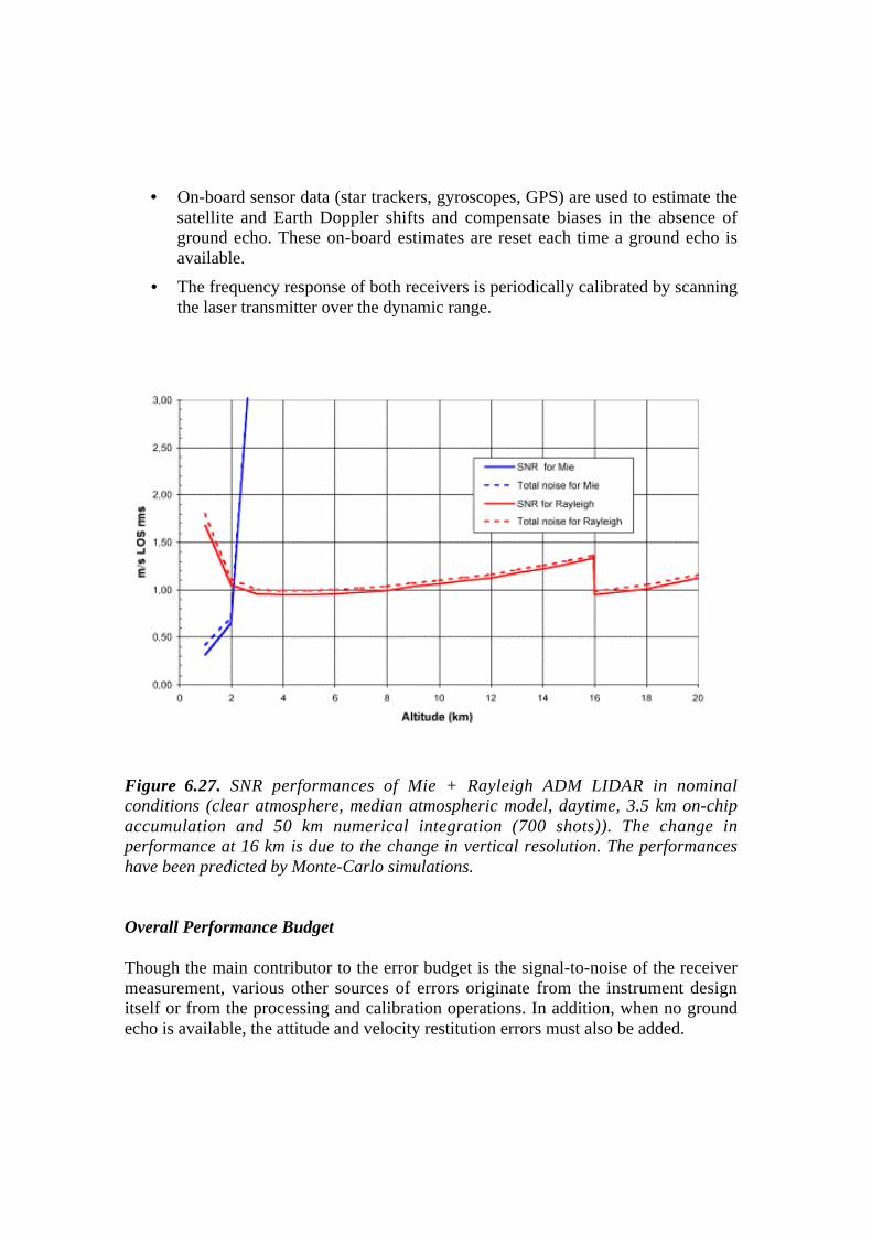
• On-board sensor data (star trackers, gyroscopes, GPS) are used to estimate thesatellite and Earth Doppler shifts and compensate biases in the absence ofground echo. These on-board estimates are reset each time a ground echo isavailable.

• The frequency response of both receivers is periodically calibrated by scanningthe laser transmitter over the dynamic range.

Figure 6.27. SNR performances of Mie + Rayleigh ADM LIDAR in nominalconditions (clear atmosphere, median atmospheric model, daytime, 3.5 km on-chipaccumulation and 50 km numerical integration (700 shots)). The change inperformance at 16 km is due to the change in vertical resolution. The performanceshave been predicted by Monte-Carlo simulations.

Overall Performance Budget

Though the main contributor to the error budget is the signal-to-noise of the receivermeasurement, various other sources of errors originate from the instrument designitself or from the processing and calibration operations. In addition, when no groundecho is available, the attitude and velocity restitution errors must also be added.

93

The main contributors to the overall system error include the following:

• The SNR error relates to the effect of detection noise statistic and windretrieval algorithm. This is by far the biggest contributor to the overall errorbudget.

• Medium-Resolution etalon stability relates to distortion induced by anymedium-resolution etalon spectral transmission decentre on the molecularreturn spectral shape. It affects the molecular channel only.

• The Rayleigh spectrum shape affects the molecular channel response throughspectrum width variation due to probed air volume temperature and spectrumshape distortion due to the Brillouin effect.

• The Background processing relates to the after post-processing residual errorinduced by the Medium-Resolution etalon on the spectral shape of thebackground light. It affects the aerosol channel only.

• The Mie signal contamination models the residual aerosol return entering themolecular channel. It affects the molecular channel only.

• Ground echo accuracy relates to the calibration of the ‘zero wind’ using theaerosol channel and the ground return.

• Internal calibration accuracy refers to the ‘zero’ inter-channel calibration errorusing a laser pulse emitted internally on both channels.

• Response calibration accuracy refers to the error on the spectral calibrationusing an internal laser pulse swept in frequency over the useful spectral rangeof both channels.

• The Sensor/LOS alignment stability refers to the determination of LOS Earthand satellite Doppler shifts extrapolated from onboard sensor data and usedwhen the ground echo is not available. Thermo-elastic behaviour of theinstrument structure as well as attitude restitution stability, over half an orbit inthe worst case, are at the origin of this contributor.

The system performance presented below includes all of the errors described above.This performance considers the SNR error for each channel at the indicated altituderange. Systematic bias errors (correlated errors between profiles) are also considered.The calculations are based on the pointing performances described in Section 6.4.4.

Mie channel @ 2 km Rayleigh channel @ 10 km

Measurement accuracy (noise + bias) 0.67 m/s 1.05 m/s

Table 6.5. Instrument overall LOS performance (with ground echo).

When no ground echo is retrieved, the measurement bias is not cancelled and the totalmeasurement error is slightly deteriorated (Table 6.6). However, this worst case isbased on the assumption that ground echoes are only available twice per orbit. This isvery unlikely to happen and will not significantly influence the mission performance.

Mie channel @ 2 km Rayleigh channel @ 10 km

Measurement accuracy (noise + bias) 0.85 m/s 1.23 m/s

Table 6.6. Instrument overall LOS performance (without ground echo).

For the Mie channel, the LOS wind error is below the requirement of 0.6 m/s from 0 to2 km height. The reliability is around 100% in the same altitude region. For theRayleigh channel, the LOS wind error is below the requirement, except for a marginalperformance around the height of 16 km (leading to a slight exceeding of therequirements in one altitude layer, which is not considered critical to overall missionperformance).

As explained in 6.2.2, the orbit height has an impact on the overall systemperformance. There is however considerable system margin that would allow theperformance to be improved by e.g. reducing the orbit altitude. The fuel assumed inthe system budget would allow the spacecraft to fly at 360 km altitude. This altitudewould provide a potential improvement in the range of 0.2 m/s in the HLOS velocityerror.

Flexibility

Thanks to the implementation of a programmable sequencer for the detector, thealtitude vertical resolution and range can be changed in-flight during the course of themission. The vertical resolution can be varied from 100 m to 2 km or more and there isno limitation on the altitude range. The horizontal accumulation length can also bechanged during the mission. This length can be varied from 500 m (Mie or Rayleigh)to 50 km without performance degradation for the required horizontal integrationlength of 50 km. The lower value of the accumulation length is mainly limited by theCCD read-out noise. This capability will be used to implement the processing strategyoutlined in Section 7.2.

Instrument Resource Budget Estimates

The overall mass of the instrument concept (instrument core + top panel electronics) is263 kg, which includes design margins according to the maturity of the components.The average power consumption is 304 W average (with 25% laser duty cycle,assuming full heater power). The main contributor to the power budget is the laser.

95

The data rate is very low (11 kbps in the most demanding case) due to the opticalaccumulation principle of the receiver. The overall instrument envelope fits withinvarious launcher fairings, with several hundred millimetres margin at the baffle level.

6.4 The Satellite

6.4.1 Satellite Configuration

Derived Requirements

The main system demands on the satellite are to fly in a Sun-synchronous dawn-duskorbit of 400 km altitude, and to carry a continuously operated lidar instrument(ALADIN) whose main field of view is 35° off nadir to the anti-Sun side of thesatellite track.

The performance requirements of the instrument mean that an optical aperture of1.1 m is needed, resulting in an outer diameter for the protecting baffle of about 1.2 mdiameter, which dictates to some extent the dimensions of other satellite elements. Afurther consequence of the measurement performance requirements is the need toprovide an excellent thermal stability, which affects the distribution of the units in thesatellite.

An important factor in the satellite layout is the desire to minimise drag at the altitudechosen, in order to minimise fuel consumption for orbit maintenance (Section 6.2.2).The whole concept must also be capable of being launched by the smallest/cheapestpractical launcher.

Description of Selected Concept

A baseline configuration has been selected after an extensive analysis and trade-off ofseveral candidates. The design features of the selected baseline concept are shown inFigure 6.28. The satellite consists of a bus as a conventional box structure with centralcone (Fig. 6.30), upon which the instrument is mounted via the three isostatic mounts(bipods). This assembly is flown with the instrument pointing down in a planeperpendicular to the flight path and 35 degrees offset from nadir in the anti-Sundirection (see Fig. 6.1). Since the satellite is flown in a dawn-dusk orbit, the y-sidealways faces away from the Sun, and the solar arrays can be wings, one forward andone aft of the bus (with reference to the flight direction), fixed in orientation.

The advantages from the thermal design point of view are significant, since thisensures that no direct sunlight enters the instrument baffle under operationalconditions, assisting in instrument stability. The thermal conditions are effectively

stable for the whole mission lifetime, especially as there are eclipses only for a periodof about 4 months.

Figure 6.28. Deployed satellite configuration of selected baseline.

The anti-Sun face of the satellite can be dedicated to the instrument radiators, relievingthe baffle of additional structural demands. The use of this bus panel has been madepossible by arranging the bus electronic units on the inside of the flight and anti-flightfaces of the bus. These latter two faces can also form all the radiative surfaces wherenecessary for the bus electric units. With the (in-flight) lower face of the bus carryingthe instrument, the opposite face can easily accommodate the launcher attachmentinterface. This establishes an easy and optimum load path from the instrument isostaticmounts through the central structural tube to the launcher. The resulting configurationis shown in the views presented in Figure 6.29.

97

Figure 6.29. Different views of baseline configuration.

Structure

The selected bus structure design consists of a central cone, feeding the launch loadsof the instrument directly to the launch adapter on the bottom. Four side walls areattached to the cone by flat shear walls. This design makes it possible to mount allelectronics boxes of the bus and associated satellite equipment onto only two sidepanels. In addition, these +x and –x panels serve directly as radiators for dissipatingthe heat of the bus equipment.

The +y and –y panels do not carry internally mounted equipment, thus offering easyaccess during satellite assembly and test. All structural elements are made ofaluminium honeycomb.

Figure 6.30. Main satellite components.

Subsystem Layout

As depicted in Figure 6.31, the units mounted internally on the bus are generallygrouped on the flight and anti-flight walls of the bus (+/-x). This enables the centre ofgravity to be easily placed near the launcher axis of symmetry. Exceptions to this arethe instrument electronics, the thrusters and the reaction wheels. The star trackers aredirectly mounted on the primary structure close to the instrument optics.

To limit the cable length, the instrument electronics are mounted close to theinstrument on the inside of the top face (+z) of the bus and on the upper parts of the

99

+/-x panels. This aspect must be closely controlled, as space is at a premium, theintention being to minimise the bus volume to reduce drag cross-section.

Figure 6.31. Unit layout of the satellite bus panels.

The propulsion equipment can be completely accommodated inside the central tube.The tank will be situated as near as possible to the CoG and mounted directly on thetube walls. The thruster group can be placed inside the launcher adapter ring on thelower face (-z) of the bus. The maximum capacity of the tank is bigger than needed forthe approximately 60 kg of fuel required.

The four reaction wheels are mounted directly on the lower face of the bus, outside thecentral tube area, at angles suitable to the optimisation of the AOCS function.

Because of the dawn-dusk orbit, the solar arrays will have a fixed orientation whendeployed. No tracking mechanism is required, as justified in 6.2.4. The deploymentmechanism will be designed to ensure orientation of the arrays at 10° to the orbitalplane.

The L-band data link antenna is a design derived from the high-resolution picturetransmission standard (HRPT) defined for METOP. This requires an antenna which isnadir pointing, with a field of view cone up to 70 degrees from nadir. The optimumplace for the antenna is on the bottom lip of the instrument baffle, mounted in a waywhich minimises stray-light reflections into the baffle. The lower S-band TT&Cantenna must also have a field of view covering the lower hemisphere, i.e. itsboresight has to point near to nadir. By placing the antennas on either side of thebaffle, both antennas can be adequately installed.

The upper S-band TT&C antenna is correspondingly tilted in boresight to cover theother hemisphere, so it must be placed on the opposite upper corner of the bus. TheGPS antennas, being patch antennas, can be mounted on the upper edge of the bus.The antenna locations can be seen in Figure 6.28.

The design of the satellite has not conflicted with the demands of the launcherenvelope of the baselined Rockot launcher candidate. Consequently, for convenienceof design and sizing of the bus central tube, the ‘standard’ interface diameter of937 mm has been chosen, allowing a significant degree of alternative launcher choicewithout the need to rethink the satellite concept.

6.4.2 Thermal Architecture

Overall Thermal Architecture and Constraints

The overall thermal architecture is based on the definition of a simple thermalinterface between instrument and bus, with no heat flux between instrument and busthrough the structure. As shown in Figure 6.30, the bus incorporates on the +/-x panelsthe radiators for the bus electronic boxes, including a separate radiator for the battery.In addition to the bus components, the bus houses the instrument electronic boxes andthe relevant radiator, located on the +y panel. The radiators of the power laser headand a common radiator for the optical bench and the reference and seed laser head arealso located on the +y panel. The dissipation heat of all these instrument componentsis transported to the radiators via heat pipes.

The temperatures of all sensitive components are stabilised with dedicated smallheater systems, consisting of heaters, thermistors and electronic control. Wherenecessary, these components are insulated against their support structures and internalsurroundings.

Instrument

Because of the required temperature stability in some instrument components, thewhole radiator area foreseen for the instrument is located on the +y side, which always

101

views deep space and offers a relatively constant heat-sink temperature. Theseradiators are located on the bus panel in order to save weight and to minimise thethermal impact on the baffle internal gradient. The baffle employs a segmented heatersystem to meet the required temperature stability. The heat generated within the baffleis radiated directly through its insulation.

The instrument boxes are fixed to the optical bench or the primary structure. They areall thermally insulated against the support structure and its surrounding. Theirdissipation heat is transported via L-shaped heat pipes to the three +y radiator panels.The expected thermal dissipations at the element groups are summarised in Table 6.7.The overall required dissipation heat is 294 W and as the +y panel is able to dissipateon its 1.7 m2 surface about 540 W so that this panel is partially insulated with MLIsheets. For the power laser head boxes, a cold-redundancy concept will be applied.Both boxes are combined to the same radiator so that the active box is dissipating tothe radiator and some heat is fed back to the inactive box via reverse working heatpipes to hold this box at the required temperature level.

Item Power [W]

Radiator for instrument electronic boxes 157

Radiator for Power Laser Head (PLH) 125

Radiator for optical bench and seed laser boxes 12

Total 294

Table 6.7. Thermal dissipation of instrument components.

The dissipation heat of the optical bench and the reference laser head, mentionedabove, also includes the heat produced by the small auxiliary heater system, whichhelps stabilise the temperature of these components. The thermal design allowsanalysis and testing of the individual boxes without having to account for any impactfrom the overall environment and structure.

Satellite Bus

The overall heat dissipation of the bus is about 215 W including the battery heatdissipation. As the bus electronics are not very sensitive to temperature stability, theheat of the bus will be radiated via the +/-x panels. These two panels, each with a1.7 m2 surface area, are able to dissipate much more heat than required (consideringalso an albedo effect and a seasonal solar incidence angle of up to 30°) and arepartially covered with MLI, allowing in addition final adjustments during system tests.

All bus boxes are directly fixed to the inner side of these +/- x panels so that theirdissipation heat can be conducted through the panel and radiated on this opposite side.

The battery will be accommodated on a thermally but not mechanically de-coupledradiator panel due to its lower operation temperature. Thus, the thermal design of thebus is based on standard tools and hardware without special risks or developmentrequirements.

6.4.3 Electrical Architecture

The overall electrical architecture of the ADM satellite as shown in Figure 6.32 iscomposed of the avionics subsystem, the electrical power subsystem (EPS) with solargenerators and interconnecting harness, the telemetry, tracking and commandsubsystem (TT&C), the payload data transmission subsystem (PDTS), and finally thethermal-control electrical equipment.

Figure 6.32. Overall electrical functional block diagram.

The avionics subsystem includes classical control & data management system(CDMS) and the attitude and orbit control system (AOCS) assembly with all sensorsand actuators. The avionics assembly has an integrated avionics processor systemsharing the processor for the CDMS and the AOCS tasks.

103

Dedicated internal functional/electrical interfaces to the satellite bus equipment andthe ALADIN instrument are controlled by the CDMS via serial links. A limitednumber channels as pulse commands and analogue and digital inputs will be requiredaccording to the need of the units.

The Electrical Power Subsystem (EPS) is realised by the Power Control andDistribution Unit (PCDU), a NiCd battery and the solar array. The PCDU and solararray are designed for the selected hybrid power subsystem design.

The telemetry, telecommand and tracking (TT&C) subsystem is a standard S-bandsystem with two transponders, two low gain antennas providing omnidirectionalcoverage, and a Radio Frequency Distribution Unit (RFDU). The payload datatransmission subsystem (PDTS) will transmit the science data in L-band.

Electrical equipment for thermal control are heater mats, thermistors, thermal-controlpower outlets in the PCDU and thermostats for survival heater power switching.Nominally the temperature control is performed via software-controlled circuits.

Avionics Subsystem

The avionics architecture is defined in Figure 6.33 and represents a subsection of theoverall electrical architecture. The major elements, their functions andimplementations are summarised below.

Figure 6.33. Avionics architecture.

The CDMS consists of one redundant ERC 32 Processor (SPARC) with Packet TCDecoder, Transfer Frame Generator (Packet TM), Reconfiguration Module andSafeguard Memory, System Clock, and Solid State Mass Memory (SSMM) forinstrument data storage. The functions to be provideed are command, telemetry,overall spacecraft control, and timing facilities, dedicated AOCS/RCS control-lawimplementation, and required data storage during all phases of the mission.

The software will consist of the real-time operating system software (VxWorks asbaseline) and dedicated application software, in charge of data management andAOCS tasking. The SSMM will be implemented as 256 Mbit RAM, with direct accessto the bus of the CDMS.

Serial end-to-end links are selected for the interface: IEEE 1355 links to the AOCSInterface Unit (AIU) and the instrument, RS 422 to the non-intelligent users like theElectrical Power Subsystem and the RTU. A standard RTU will provide limited pulsecommands distribution and analogue and digital status acquisition.

Direct clock and time-reference distribution to the ALADIN Instrument will beprovided and implemented as 1 Hz clock with UTC datation and a 20 MHz clock inthe instrument.

The AOCS assembly comprises all relevant sensors and actuators with their respectiveinterfaces. These interfaces are connected to the common AIU with autonomousswitching capabilities for primary power and elementary failure handling functions.The AOCS application software (e.g. control laws) will be running in the CDMSprocessor.

Electrical Power Subsystem (EPS)

The EPS design is mainly driven by the laser pulse power and the instrument detectorrequirements. The laser needs 100 Hz peaks in the kW range, for periods of 7 s andabout 1 s for warming up. The power subsystem must comply with laser power forpulsed, diode-pumped solid-state laser technology. The detector power supply has tobe free of ripples.

The dawn-dusk orbit determines the battery layout by the worst-case eclipses insummer solstice.

The EPS and solar generator interface architecture as depicted in Figure 6.34 isselected as a baseline. It includes an hybrid power bus mainly because of EMCreasons offering a regulated primary power bus and a direct battery buffered outlet forthe laser pulse power. The main characteristics of the elements of the EPS are listed inTable 6.8. All power units are based on existing designs, with flight-proventechnologies.

105

Figure 6.34. Baseline for Electrical Power Subsystem (EPS).

Solar Array • Fixed wings; parallel strings connected to sections• 12 main power bus sections + one section for redundancy• 8 battery charge sections + one section for redundancy• 920 W EOL• Si-BSFR cells, 8.4 m2 total wing area• 2 x 10 kg

Power Conditioning andDistribution Unit (PCDU)

• Power control module for hybrid power bus concept with S3Rfor main bus power- Separate switches for battery charging, controlled by

battery charge status- Battery discharge regulation in eclipse- Power of charge array sections can be switched directly on

to the main power bus- PCDU power bus recovers automatically from any

shutdown transition if the cause of it is disappeared• Power distribution module including

- Pyro module- Latching current limiters in line with the protective

switchesOne NiCd Battery • 28 cells in line

• 18 Ah• 25.5 kg• The battery layout is mainly for LEOP power service and for

high current flow for the laser peak power• The eclipse power DOD is < 40%.

Table 6.8. Main characteristics of the Electrical Power Subsystem (EPS).

Tracking, Telemetry and Command (TT&C) Subsystem

The TT&C subsystem consists of all elements for RF reception, demodulation,modulation and transmission. The fundamental functions are to receive up-link signalsfor telecommand purposes, and to transmit down-link telemetry signals. In addition,ground tracking is supported.

The RF-subsystem comprises two low-gain antennas (for omni-directional coverage),an RF-distribution network (RFDU), consisting of two transfer switches andRF-harness, and two S-band transponders, each consisting of a receiver, a transmitterand a diplexer. The block diagram shown in Figure 6.35 illustrates the subsystemconfiguration, implemented with off-the-shelf hardware.

The max. 64 kbps downlink rate can be handled with a link margin here of more than4 dB. The required RF power is minimal (3 mW). For the telecommand channel of2 kbps the link margin is bigger than 50 dB.

Figure 6.35. TT&C subsystem functional configuration.

Payload Data Transmission Subsystem (PDTS)

In order to benefit from existing ground and on-board terminals, the L-band link – asused for HRPT of METOP – has been selected for PDT.

The PDT consists of two transmit chains in cold redundancy configuration composedof an internally redundant modulator assembly containing an encoder section, a pulse-shaping filter, a modulation section and an up-conversion section, an L-band solid-state power amplifier (SSPA). A switch connects the active chain to the filter and the

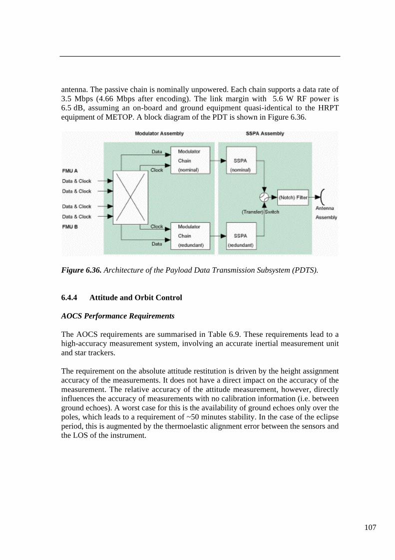
107

antenna. The passive chain is nominally unpowered. Each chain supports a data rate of3.5 Mbps (4.66 Mbps after encoding). The link margin with 5.6 W RF power is6.5 dB, assuming an on-board and ground equipment quasi-identical to the HRPTequipment of METOP. A block diagram of the PDT is shown in Figure 6.36.

Figure 6.36. Architecture of the Payload Data Transmission Subsystem (PDTS).

6.4.4 Attitude and Orbit Control

AOCS Performance Requirements

The AOCS requirements are summarised in Table 6.9. These requirements lead to ahigh-accuracy measurement system, involving an accurate inertial measurement unitand star trackers.

The requirement on the absolute attitude restitution is driven by the height assignmentaccuracy of the measurements. It does not have a direct impact on the accuracy of themeasurement. The relative accuracy of the attitude measurement, however, directlyinfluences the accuracy of measurements with no calibration information (i.e. betweenground echoes). A worst case for this is the availability of ground echoes only over thepoles, which leads to a requirement of ~50 minutes stability. In the case of the eclipseperiod, this is augmented by the thermoelastic alignment error between the sensors andthe LOS of the instrument.

Xo Yo Zo

Attitude (in µrad rms)

ControlPointing 520 520 520Stability over 3 ms 0.5 0.33 0.33Stability over 0.5 s – 2 2Stability over 7 s 300 2 2

RestitutionAbsolute 130 – –Relative 10 10 10

Orbit (rms)

RestitutionPosition (in m) 20 20 20Velocity (in m/s) 0.067 0.067 0.067

Table 6.9. AOCS performance requirements summary.

AOCS Modes

The AOCS modes and their transitions are simplified to minimise the operationalcomplexity. These modes, depicted in Figure 6.37, are the same as considered in theLeostar avionics development and have already been validated in a multi-missionframework. Detailed simulations with existing development tools have shown that theADM can be handled within the existing hardware and software, which gives a highlevel of confidence in the results presented below.

The Idle mode is used during ground integration and during the launch. After launcherseparation, the launcher induced altitude rates are damped in less than 15 minutes by astandard rate reduction mode, using only a magnetometer, the wheels and the thrustersfor a fast convergence. Afterwards, the solar arrays will be deployed.

The satellite then enters its Acquisition and Safe Hold (ASH) mode. The ASH is usedfor initial attitude acquisition. The ASH uses the minimum possible hardware,avoiding in particular gyroscopes and thrusters, which gives a particularly simple,robust and autonomous mode. Moreover, this mode does not use consumables, is nottime-limited, and does not disturb the orbit. In this mode, the satellite is oriented insuch a way that the solar arrays points towards the orbit normal, i.e. near the Sundirection, and slowly rotates around this axis. The ASH is also used in the case ofemergency.

109

After ground authorisation, the transition mode is entered. In this mode, the fineattitude sensors, which consist of gyros and star trackers and the onboard navigator,will be initialised on the basis of ground data. After attitude-estimation convergence,the satellite will autonomously point to the Earth. It then initiates the GPS receiver invery secure conditions. At the end of this mode, the satellite is Earth-pointing and canenter the normal mode.

Figure 6.37. AOCS modes and transitions.

The normal mode is the mode in which the satellite will spend its operational life.During this mode, the satellite points its Zo axis towards the Earth. The Xo axis pointsto the satellite velocity direction and modulated with the required yaw steering angle.In this mode the satellite is controlled by the reaction wheels, which are periodicallyoff-loaded by the magnetic torquers.

The orbit-control mode is used to control and adjust the orbit. In this mode, thesatellite is controlled as in normal mode, but the thrusters are used to provide therequired boost.

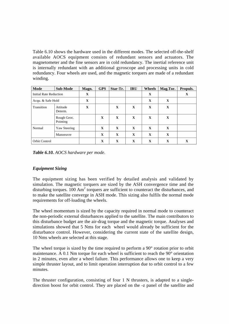
Table 6.10 shows the hardware used in the different modes. The selected off-the-shelfavailable AOCS equipment consists of redundant sensors and actuators. Themagnetometer and the fine sensors are in cold redundancy. The inertial reference unitis internally redundant with an additional gyroscope and processing units in coldredundancy. Four wheels are used, and the magnetic torquers are made of a redundantwinding.

Mode Sub-Mode Magn. GPS Star-Tr. IRU Wheels Mag.Tor. Propuls.Initial Rate Reduction X X X

Acqu. & Safe Hold X X X

Transition AttitudeDeterm.

X X X X X

Rough Geoc.Pointing

X X X X X

Normal Yaw Steering X X X X X

Manoeuvre X X X X X

Orbit Control X X X X X X

Table 6.10. AOCS hardware per mode.

Equipment Sizing

The equipment sizing has been verified by detailed analysis and validated bysimulation. The magnetic torquers are sized by the ASH convergence time and thedisturbing torques. 100 Am2 torquers are sufficient to counteract the disturbances, andto make the satellite converge in ASH mode. This sizing also fulfils the normal moderequirements for off-loading the wheels.

The wheel momentum is sized by the capacity required in normal mode to counteractthe non-periodic external disturbances applied to the satellite. The main contributors tothis disturbance budget are the air-drag torque and the magnetic torque. Analyses andsimulations showed that 5 Nms for each wheel would already be sufficient for thedisturbance control. However, considering the current state of the satellite design,10 Nms wheels are selected at this stage.

The wheel torque is sized by the time required to perform a 90° rotation prior to orbitmaintenance. A 0.1 Nm torque for each wheel is sufficient to reach the 90° orientationin 2 minutes, even after a wheel failure. This performance allows one to keep a verysimple thruster layout, and to limit operation interruption due to orbit control to a fewminutes.

The thruster configuration, consisting of four 1 N thrusters, is adapted to a single-direction boost for orbit control. They are placed on the -z panel of the satellite and

111

used only for orbit maintenance in nominal operations. However, it is possible toproduce the torques required for rate reduction after launch by actuating them in pairs.

AOCS Performances

The AOCS performance is mainly a function of the sensors, and at a lower level of thewheel vibrations. The pointing control performance, as simulated for the 400 km orbit,easily fulfils the requirements, mainly because the sensors are mounted on theinstrument, thus minimising their relative thermal distortion. The stability over 7 s willeasily be fulfilled, because it is applicable only to non-zero variations over this timeperiod, i.e. to frequencies lower than 0.2 Hz involving only a part of the gyro-star-tracker noise and GPS filtered noise. The same is true for the 0.5 s requirement, whichinvolves only frequencies lower than 1 Hz and a small part of the gyro-star-trackernoise.

The stability requirement over 3 ms applies only to high frequencies and thereforeonly to wheel vibration. A first worst-case computation has shown that if the wheelunbalance is in the range of 0.1 g·cm and the harmonics stay at a similar magnitude,the requirement of 0.33 µrad can be met.

The attitude-restitution requirements are the main drivers. The absolute attitude-restitution requirement is applicable around the satellite roll axis and can marginallybe met. The remaining biases, caused by thermal and mechanical distortions betweenthe star tracker and the instrument LOS, are the main contributors to the resultingperformance.

The attitude-restitution requirements over 50 minutes can be met, because the attitudepropagation is very accurate due to the high-performance characteristics of the inertialunit. The worst-case calculation has shown that the requirements can be fulfilled alsoin the case of eclipses.

The orbit-restitution requirements will also be easily fulfilled with standard equipmentand adequate filter algorithms.

Comparing Table 6.11 and Table 6.9 shows that the AOCS requirements are met. Theabsolute restitution in roll requirement is marginal and leads to a slightly higher heightassignment error. However, this is still judged to be sufficient to achieve the missionobjectives. The worst case for the relative restitution is non-compliant. However, thissituation is judged to be very unlikely (half an orbit without any ground echo) and canonly occur in the three months around the summer solstice, where the thermaldistortion effects are maximal due to the eclipse.

Xo Yo Zo Errors type

Attitude (in µrad rms)

Control

Pointing 190 230 210 All

Stability over 3 ms < 0.3* < 0.3* < 0.3* Noise

Stability over 0.5 s for frequencies lower than 2 Hz 0.2 0.2 0.2 Noise

Stability over 7 s for frequencies lower than 0.2 Hz** 2.0 2.0 2.0 Noise

Restitution

Absolute restitution without eclipse 160 210 180 All

Absolute restitution with eclipse 190 220 210 All

Relative restitution over 2 min 0.9 0.9 0.9 Noise

Relative restitution over 50 min out of eclipse 18 21 20 Thermal +noise***

Relative restitution over 50 min with eclipse orbit 46 34 41 Thermal +noise***

Orbit (rms)

Restitution

Position (in m) 20 20 20 Noise

Velocity (in m/s) 0.033 0.033 0.033 Noise

* with wheels balanced to about 0.1 g·cm and equivalent other harmonics** with control bandwidth greater than 0.2 Hz*** The values include the misalignment between the sensors and the LOS (compatible with the assumptions inSection 6.3.2).

Table 6.11. AOCS performance summary.

Type Equipment Nbr Main Characteristics Technology Redundancy

Sensors Magnetometer 2 3-axis Fluxgate Cold Redundancy

GPS Antennas & pre-amps 2 Half-space coverage Patch Antenna Cold Redundancy

GPS Receiver 2 C/A GPS Receiver RF ASIC and µProc Cold Redundancy

Star Tracker 2 Large Field of View CCD Cold Redundancy

Inertial Reference Unit 1 3 measurement axes HRG Internal

Actuators Reaction Wheels 4 10 Nms / 0.1 Nm Ball Bearings 3 among 4

Magnetic Torquers 3 100 Am2 Windings Cold Redundancy

Table 6.12.. AOCS hardware and redundancy matrix.

6.4.5 Satellite Budgets

Table 6.13 shows a launch mass of the ADM satellite of 785 kg, which is fullycompatible with the baseline launcher Rockot for the selected 400 km Sun-synchronous orbit. This figure already includes 100 kg of fuel for a mission lifetime of3 years plus one additional year for consumables. In addition, the budget includes thestandard maturity factors for the selected equipment, depending on their design status.

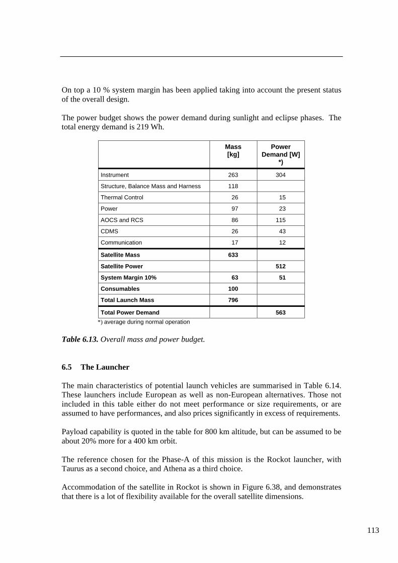
113

On top a 10 % system margin has been applied taking into account the present statusof the overall design.

The power budget shows the power demand during sunlight and eclipse phases. Thetotal energy demand is 219 Wh.

Mass[kg]

PowerDemand [W]

*)

Instrument 263 304

Structure, Balance Mass and Harness 118

Thermal Control 26 15

Power 97 23

AOCS and RCS 86 115

CDMS 26 43

Communication 17 12

Satellite Mass 633

Satellite Power 512

System Margin 10% 63 51

Consumables 100

Total Launch Mass 796

Total Power Demand 563

*) average during normal operation

Table 6.13. Overall mass and power budget.

6.5 The Launcher

The main characteristics of potential launch vehicles are summarised in Table 6.14.These launchers include European as well as non-European alternatives. Those notincluded in this table either do not meet performance or size requirements, or areassumed to have performances, and also prices significantly in excess of requirements.

Payload capability is quoted in the table for 800 km altitude, but can be assumed to beabout 20% more for a 400 km orbit.

The reference chosen for the Phase-A of this mission is the Rockot launcher, withTaurus as a second choice, and Athena as a third choice.

Accommodation of the satellite in Rockot is shown in Figure 6.38, and demonstratesthat there is a lot of flexibility available for the overall satellite dimensions.

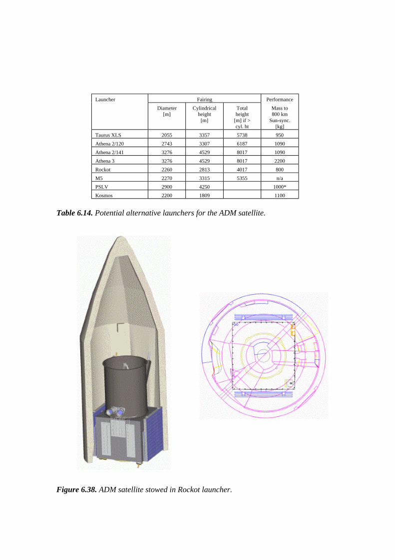
Launcher Fairing Performance

Diameter[m]

Cylindricalheight

[m]

Totalheight

[m] if >cyl. ht

Mass to800 km

Sun-sync.[kg]

Taurus XLS 2055 3357 5738 950

Athena 2/120 2743 3307 6187 1090

Athena 2/141 3276 4529 8017 1090

Athena 3 3276 4529 8017 2200

Rockot 2260 2813 4017 800

M5 2270 3315 5355 n/a

PSLV 2900 4250 1000*

Kosmos 2200 1809 1100

Table 6.14. Potential alternative launchers for the ADM satellite.

Figure 6.38. ADM satellite stowed in Rockot launcher.

115

The launch related activities begin with the pre-launch phase, where the satellite willbe shipped to the launch site in Plesetsk, mated to the launch vehicle, followed by afinal pre-launch check-out. The launch campaign will last about one month.

The ensuing Launch and Early Orbit Phase (LEOP) is divided into the launch and theacquisition phase (initial rate reduction phase and Sun-pointing phase). Thecountdown and launch sub-phase lasts from the start of the countdown, through thelift-off, and until the separation of the satellite from the launch vehicle. The upperstage of the Rockot launcher, the so-called Breeze stage, can provide any requiredpayload attitude. The specified 3 σ attitude error along each spacecraft axis, as well asthe angular velocity after separation, are specified and well within the capabilities ofthe selected AOCS.

Directly after separation, the initial rate reduction starts, using the magnetometer assensor and possibly the thrusters as actuators, in order to reduce the angular velocityfor safe solar-array deployment. This is followed by the solar-array deployment andinitialisation of the ASH mode.

6.6 The Ground Segment

6.6.1 Ground Segment Design Guides

The major functions of the ground segment are to:

• monitor and control the satellite, including the payload and the ground-segment elements

• receive the instrument data from the satellite, and

• process, disseminate and archive the data and products, and provide for theirretrieval.

The key requirements state that the Level 1 products shall be available at the ScienceData Processing Centre within 3 hours of observation, with a reliability of 95%. ThisScience Data Processing Centre will produce the Level 2 products and the associatedprocessor software, and disseminate this through a network to the meteorological aswell as other scientific users. The delivery of Level 1 products for other users will bedone upon request. There will be the possibility to order these archived products viathe Internet.

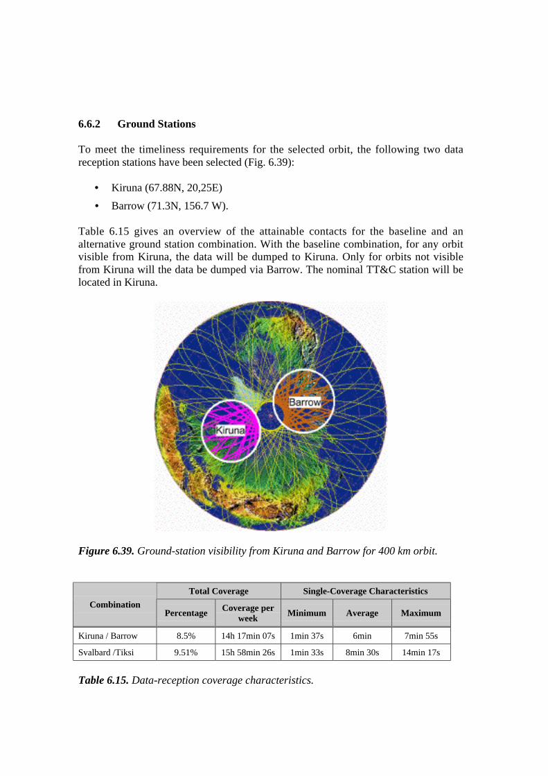
6.6.2 Ground Stations

To meet the timeliness requirements for the selected orbit, the following two datareception stations have been selected (Fig. 6.39):

• Kiruna (67.88N, 20,25E)

• Barrow (71.3N, 156.7 W).

Table 6.15 gives an overview of the attainable contacts for the baseline and analternative ground station combination. With the baseline combination, for any orbitvisible from Kiruna, the data will be dumped to Kiruna. Only for orbits not visiblefrom Kiruna will the data be dumped via Barrow. The nominal TT&C station will belocated in Kiruna.

Figure 6.39. Ground-station visibility from Kiruna and Barrow for 400 km orbit.

Total Coverage Single-Coverage Characteristics

CombinationPercentage Coverage per

weekMinimum Average Maximum

Kiruna / Barrow 8.5% 14h 17min 07s 1min 37s 6min 7min 55s

Svalbard /Tiksi 9.51% 15h 58min 26s 1min 33s 8min 30s 14min 17s

Table 6.15. Data-reception coverage characteristics.

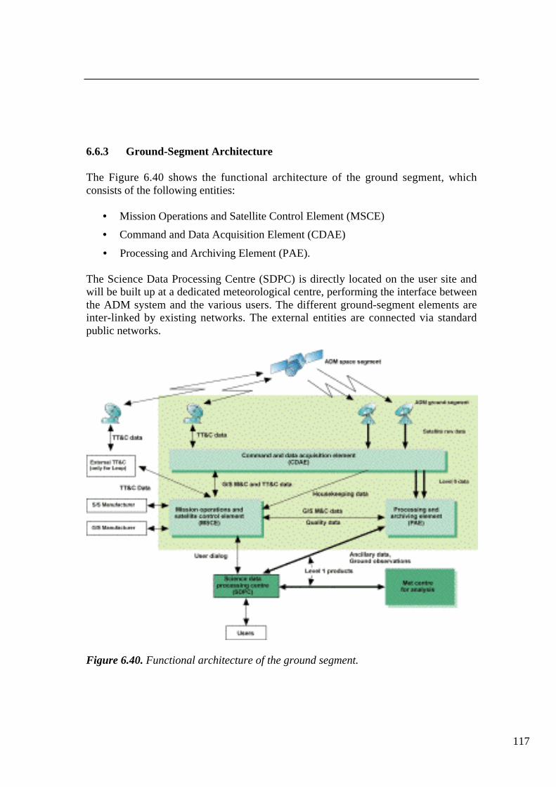
117

6.6.3 Ground-Segment Architecture

The Figure 6.40 shows the functional architecture of the ground segment, whichconsists of the following entities:

• Mission Operations and Satellite Control Element (MSCE)

• Command and Data Acquisition Element (CDAE)

• Processing and Archiving Element (PAE).

The Science Data Processing Centre (SDPC) is directly located on the user site andwill be built up at a dedicated meteorological centre, performing the interface betweenthe ADM system and the various users. The different ground-segment elements areinter-linked by existing networks. The external entities are connected via standardpublic networks.

Figure 6.40. Functional architecture of the ground segment.

Mission Operations and Satellite Control Element (MSCE)

The MSCE is the core of the ADM ground segment. Its task is to operate the spacesegment and the ground segment. Among others, it performs the following functions:

• Mission Operations

• Satellite Operation, Monitoring and Control

• On-Board Software Maintenance, and

• System Performance Evaluation.

It is planned that the MSCE will be realised and operated at ESOC in Darmstadt.ESOC will have available all tools required to execute the tasks mentioned above. Forflight dynamics, the Orbit Attitude Operations System called ORATOS will be used,which has already been employed for a number of different missions. For all othertasks mentioned above, the SCOS 2000 system is presently being developed and willbe operational before the end of 1999.

Command and Data Acquisition Element (CDAE)

The CDAE is divided into the:

• TT&C station, and

• data-acquisition stations.

The TT&C station is the interface between the satellite and the ground segment for theexchange of satellite housekeeping data and the uplinking of telecommands includingsoftware upgrades to the satellite. For nominal operation, the housekeeping telemetryreception and the telecommand transmissions will be achieved on a 24 hour cycle. Inorder to meet the required 72 h autonomy the satellite will be pre-programmedaccordingly. For contingency cases the data exchange is possible during more than68% (11 out of 16 orbits) of the orbits. For nominal operations, the ESOC TT&Cstation at Kiruna is selected. As backup, other ESA TT&C stations can be used.

The data-acquisition stations have the task of acquiring the global data stream,containing the space segment housekeeping data and the instrument observation data,and forwarding them all to the PAE and the housekeeping data to the MSCE.

For the down-linking of the instrument observation data, an L-band link offering adata rate of 3.5 Mb/s has been selected. It has been designed to be compatible with theL-band HRPT facility, presently under development in the frame of the EPSprogramme (METOP ground segment). The HRPT facilities are small remotelycontrolled stations, characterised by a parabolic tracking antenna with a 2.4 m

119

reflector and a G/T better than 6 dB/K. The electronics is implemented in a 19 inchrack system, controlled by a PC with a GPS time and frequency reference system. Inaddition, the station comprises an integrated link quality-assurance system. Thesestations are expected to be available in 2002 for METOP and can directly be installedat the Kiruna and Barrow sites.

The data and processing flow for the observation data and the centres where theprocessing will be performed is depicted in Figure 6.41. All raw data, extended byannotation data describing the restituted orbit and pointing parameters, will bearchived. The Level 1 products, characterised as geocoded wind component vectorsincluding quality-control information will be delivered not later than 3 hours afterobservation to the science data-processing centre.

Figure 6.41. Timelining of data transmission and processing.

6.6.4 Networks

For communications between the different elements of the ground segment and withexternal entities, a range of networks will be exploited, as shown in Figure 6.42. Itshows the architecture of the ADM ground segment together with the communicationnetworks.

Figure 6.42. Ground-segment architecture with networks.

121

7 Data Processing and Validation

7.1 Introduction

From Raw Data to Mission Parameter

The instrument transmits raw data to the ground segment consisting of theaccumulated spectra from the Mie receiver and the flux intensities from the Rayleighreceiver. These data are provided every 3.5 km length (nominal). Alternatively, theinstruments can provide data every 1 km for dedicated areas when required, and foreach altitude bin (-1 km to 16.5 km height for the Mie channel, 0.5 km to 26.5 km forthe Rayleigh channel). In addition to these data, laser internal calibration and theattitude data are transmitted, as well as the receiver response calibration data.

Prior to integrating data over the 50 km length, cloud detection is performed in orderto segregate the samples of clear air and those affected by cloud to control theprocessing in the presence of scattered cloud (see Section 7.4). Even in such a case thewind profile above the cloud is still obtained. Ground (or sea) echo is also searched inorder to calibrate the ‘zero wind’ when possible. If there is no echo, satellite sensordata will be used to restitute Doppler shift variations due to the attitude of the satellite.

In order to transform raw data into wind measurements processing has to be performedfor Mie and Rayleigh channels. This requires taking the radiance background and thespectrometer spectral response, as well as calibration data, into account. The decisionto use Mie or Rayleigh channel data can be based on a signal-to-noise ratio threshold.Finally, each wind measurement for each altitude layer is located in an Earth referenceframe, using satellite sensor data.

A schematic flow diagram for the data processing, calibration and validation, andinformation dissemination for the spaceborne Doppler wind lidar is shown inFigure 7.1. The various elements of this are discussed in the following subchapters, asindicated by the numbers shown to the right of each item. The particular tasks of thedata pre-processing centre are shown in Figure 7.2, explaining the various processingsteps.

Wind analyses from a dedicated meteorological centre are the final product of theADM and will be distributed to the atmospheric research community at large.However, relevant Level 0, 1, and 2 processing and products will also be generated,distributed, and archived during the ADM. The data-processing levels have beendefined by the Committee on Earth Observing Satellites (CEOS). Their definitions areshown in Table 7.1.

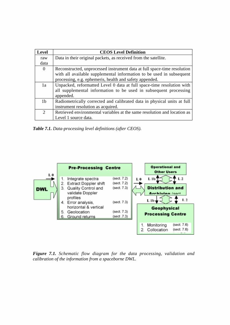
Level CEOS Level Definitionrawdata

Data in their original packets, as received from the satellite.

0 Reconstructed, unprocessed instrument data at full space-time resolutionwith all available supplemental information to be used in subsequentprocessing, e.g. ephemeris, health and safety appended.

1a Unpacked, reformatted Level 0 data at full space-time resolution withall supplemental information to be used in subsequent processingappended.

1b Radiometrically corrected and calibrated data in physical units at fullinstrument resolution as acquired.

2 Retrieved environmental variables at the same resolution and location asLevel 1 source data.

Table 7.1. Data-processing level definitions (after CEOS).

Figure 7.1. Schematic flow diagram for the data processing, validation andcalibration of the information from a spaceborne DWL.

123

Figure 7.2. The tasks of the data pre-processing centre.

The Earth Explorer ADM is a demonstration mission in several respects. Although theground processing is not very complicated, there are several aspects of the processingthat will be developed during the demonstration mission by the lidar scientificcommunity. The most important of these are discussed in this chapter.

7.2 Spectra and Doppler Frequencies

The information at Level 0 shown in Figures 7.1 and 7.2 will include all the spectraland lidar data, as well as necessary calibration and telemetry data. The spectral databasic accumulation on a shot-to-shot basis must take place in the primary detectors ofthe lidar. However, at each altitude the cloud and clear-air returns will be mixed. Forexample, an accumulation of 200 independent shots in an air layer with only 1% cloudcover gives a probability of a cloud-contaminated recording of ~ 87%. Sinceconvective clouds are broken and associated with large wind variability, it is thereforepreferrable to accumulate fewer shots at lidar detector level at one time, rapidly readthis out for processing, and then repeat the sequence of short accumulations for

eventual computation of one wind profile by integration of several accumulationprofiles.

By applying a criterion to reject primary cloud-contaminated data, the probability ofclear-air returns is increased. Additional information about the atmosphericcharacteristics in the clear (Rayleigh) and cloudy (Mie) air can be inferred from theraw primary data, and better wind-profile estimates can result from this. Primaryaccumulation over 3.5 km (at 2 Hz rate) is the nominal baseline, but accumulationover shorter distances will be investigated for further optimisation during the mission.

In this case a 50% cloud cover will generally result in only slightly over 50% cloud-contaminated primary recordings at the cloud level, which can be identified from theestimated Mie and Rayleigh SNR values. Cloud occurrence results in a somewhatdegraded Rayleigh performance over the 50 km integration length, but on the otherhand the Mie recordings for the ~ 50% of cloudy returns can potentially improve themean wind estimate at the cloud level, if both integrated detector readouts arecombined in the processing.

Extraction of Doppler frequencies from integrated spectra and recordings in groundprocessing will be carried out using already prototyped software. They are based onalgorithms taking theoretical evaluation and practical experience into account. Theserequire modest levels of computing power, will be extremely rapid and provideprocessed data (Level 1) in essentially real time. The basic outputs of such spectralprocessing will include Doppler frequency shift, strength of aerosol signal, strength ofmolecular signal, strength of noise background, assessment of statistical error,assessment of systematic or bias error, proportion of cloud contaminated data andproportion of null results.

7.3 Quality Control

7.3.1 Validation and Errors

With respect to the validation of Doppler frequencies and the associated errorassessment, two aspects need to be considered, namely statistical and systematicerrors.

The main statistical error arises from the fluctuating photon-count numbers in theaccumulated recordings. This can be dealt with in terms of the modelling andalgorithms of performance that will be developed. In particular, for the aerosol systemthese essentially random statistical errors will be mainly dependent on the strength ofthe primary back-scattered signal. The quality-control algorithms will provideguidance on the reliability as well as on the purely statistical errors in individualmeasurements.

125

On the other hand, systematic errors in derivation of the wind velocity component andheight assignment can arise in a number of ways. Vertical error correlation and profilebias can be introduced by moving particles at one altitude providing an apparent signalat another altitude. This may be due to the timing inaccuracies in the lidar, but also tothe combination of strong aerosol stratification and the laser pulse shape. These effectshave been investigated by Vaughan and Willetts (1998) for the case of typical carbon-dioxide pulse lasers. These effects are limited with short laser-pulses and a preciselycalibrated system. In addition, the assessment of aerosol signal strength and warningof severe stratification will provide a valuable safeguard against faulty assignment ofaltitude.

Another source of this error arises from any inaccuracies in the spacecraft pointing andvelocity restitution. The smaller the temporal scale of the random variations, the moredamaging its effect will be. For the ADM, the effect has been reduced by appropriateselection of the instrument configuration and LOS. A good restitution of the LOSreduces the potentially large systematic HLOS wind errors. Additionally, a calibrationwill be performed on the ground return over land and sea.

In any case, if the cloud top height is well measured then the wind-component profileabove this cloud level, measured relative to the motion of the cloud level, can beassimilated in principle. This will work well for stratiform clouds that have relativelysmall cloud dynamics and are rather uniform in cloud top height. In the case ofconvective clouds, the cloud dynamics can be substantial and the cloud top wind maynot be representative of the mean flow. However, in these situations the atmosphere isusually unstable and the clouds broken, so that for multiple shots there is a largeprobability of them reaching the Earth’s surface.

For validation and error assessment, it is planned to make use of aircraft observations.In addition, collocated radiosonde stations will be used to provide referenceobservations, a method also applied for the validation of cloud-motion winds.

7.3.2 Geolocation and Ground Returns

As emphasised above, precise knowledge of spacecraft pointing, position and velocitywill be important in minimising systematic and bias errors in the derivation ofmeasured winds. This has been discussed in Chapter 6, where detailed error budgetsare given.

However, such returns must be considered with care. For example, signals fromvegetation – crops, trees etc. – are likely to be considerably broadened by localmovement, while those from moving targets will clearly give bias errors. The seasurface is the most obvious example, in which the wave spectra develop until the mostdominant waves have the same speed as the local mean wind. Obviously the mostreliable ground returns come from bare mountain, desert and snow-field type surfaces.

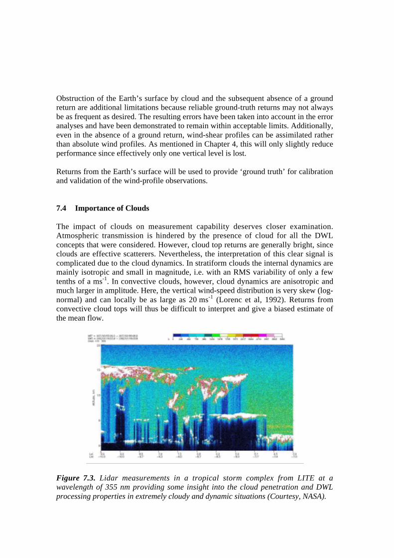
Obstruction of the Earth’s surface by cloud and the subsequent absence of a groundreturn are additional limitations because reliable ground-truth returns may not alwaysbe as frequent as desired. The resulting errors have been taken into account in the erroranalyses and have been demonstrated to remain within acceptable limits. Additionally,even in the absence of a ground return, wind-shear profiles can be assimilated ratherthan absolute wind profiles. As mentioned in Chapter 4, this will only slightly reduceperformance since effectively only one vertical level is lost.

Returns from the Earth’s surface will be used to provide ‘ground truth’ for calibrationand validation of the wind-profile observations.

7.4 Importance of Clouds

The impact of clouds on measurement capability deserves closer examination.Atmospheric transmission is hindered by the presence of cloud for all the DWLconcepts that were considered. However, cloud top returns are generally bright, sinceclouds are effective scatterers. Nevertheless, the interpretation of this clear signal iscomplicated due to the cloud dynamics. In stratiform clouds the internal dynamics aremainly isotropic and small in magnitude, i.e. with an RMS variability of only a fewtenths of a ms-1. In convective clouds, however, cloud dynamics are anisotropic andmuch larger in amplitude. Here, the vertical wind-speed distribution is very skew (log-normal) and can locally be as large as 20 ms-1 (Lorenc et al, 1992). Returns fromconvective cloud tops will thus be difficult to interpret and give a biased estimate ofthe mean flow.

Figure 7.3. Lidar measurements in a tropical storm complex from LITE at awavelength of 355 nm providing some insight into the cloud penetration and DWLprocessing properties in extremely cloudy and dynamic situations (Courtesy, NASA).

127

To facilitate the derivation of a volume-mean vector wind Stoffelen and Marseille(1998) suggest separating cloud from clear-air returns in the processing. Then, withina 50 km integration cluster, cases with anomalously large LOS wind or signal-to-noiseratio variability can be detected and assigned for dedicated processing or evenrejection. Research and development will be needed to develop algorithms thateffectively extract the useful information content of the measurements in these cases.

An example of lidar measurements from LITE in a tropical storm complex shows thateven in cases of deep convection some cloud penetration is still possible (see Fig. 7.3).

7.5 Distribution and Archiving

Part of the distribution and archiving function of the ADM ground segment isdescribed in Chapter 6; the PAE will archive the Level 1 data obtained from the DWL.Level 1 data will be processed to produce Level 2 data, which will be assimilated in ameteorological analysis. Since the volume of Level 1 data is small and the processingfrom Level 1 to 2 not very involved, it is most probable that Level 1 data will bedistributed (together with a reference processing package as is common practice) toenable Level 2 processing at the user site. This it is already common practice for manyoperational meteorological satellite instruments.

The processing centre should have the responsibility for running this referencepackage, including the functions described previously, but also for developing,maintaining and supporting this package for other users, according to therecommendations of the lidar science community. The Level 1 to 2 processingpackage will be distributed through the distribution and archiving function describedhere.

The assimilation of Level 2 data (i.e. HLOS component winds with specified errorproperties) is straightforward (Chapter 4). Since the final product of the ADM is animproved meteorological analysis, these analyses are provided by dedicatedmeteorological centres and are distributed and archived. If major updates to the groundprocessing are implemented, re-analyses of the period with DWL observations shouldbe performed, archived, and distributed. Current efforts on atmospheric re-analysis foruse in climate-related studies indicate this as a likely evolution of the ADM.

7.6 Geophysical Processing Centre

The role of the Geophysical Processing Centre (Fig. 7.1) could be taken over by ameteorological centre. They have a great capability to calibrate, validate, and monitorobserving systems (see e.g., Stoffelen, 1998, for the ERS scatterometer). Theheterogeneous data of the GOS is assimilated in such a way into a meteorologicalmodel (as depicted in Fig. 4.1) that an almost uniform quality is achieved. The error

characteristics of the meteorological model are monitored closely by comparing itagainst the observations of the GOS, and are therefore well known. As such, themeteorological model state can be compared to any DWL profile and within a fewhours sufficient statistics can be gathered to make judgements on the characteristics ofthe DWL measurements. From that moment on, useful calibration, validation, andmonitoring activities can be started at the meteorological centre, assuming a stablesystem. For this purpose, the DWL data are collocated in near-real-time with themeteorological model, but also with other observations of related quantities (i.e.radiosonde, scatterometer, cloud motion winds, and aircraft reports in the case of aDWL).

When the calibration, validation, quality assessment, and monitoring activities arefully in place, the meteorological centre will embark on meteorological analysis andforecasts which will include DWL data, in parallel with the reference operational suitewhere DWL profiles are not used (control). The first-guess field incorporating pastDWL observations will then be compared to the most recent observations in the GOS,in parallel with similar comparisons of the control first-guess. Thus, an assessmentwill be made of the improvement in the first guess due to the DWL data. A similarvalidation will be performed on the DWL and control forecasts.

If the DWL data prove beneficial for the analyses and forecasts, they will beincorporated into the operational suite. Obviously, monitoring activities will be crucialat this point, because a corruption of the analyses and forecasts due to an instrumentfailure has to be avoided. The operational use of the data signifies the most successfuldemonstration of the ADM, since forecast impact is generally only achieved after animprovement in the meteorological analyses.

The processing centre will use the collocated-observation and field products from themeteorological centre in order to validate and improve the processing. This willnecessitate ancillary information, present at the meteorological centre, to betransferred in near-real-time to the processing centre. In turn, the improvements in theprocessing or quality assessment will benefit the assimilation at the meteorologicalcentre.

In any case, the meteorological centre will eventually produce analyses in which theDWL profile data are incorporated. The scientific community at large will use theseanalyses to perform atmospheric circulation or tracer advection studies. Thedistribution and archiving centre will distribute the analysed atmospheric fields forfurther study.

129

7.7 Conclusions

The data processing and validation concept presented in this chapter is the mosteffective means of implementing the processing of the DWL observations. It relies onthe infrastructure already in place at major meteorological centres. This is expected tobe the most efficient way of establishing the required means for the end-to-endprocessing (including quality control and validation) of the ADM. The ADM willaccelerate the development of tailor-made processing algorithms and wouldconsiderably enhance the feasibility-assessment of a full-scale DWL systemmeasuring three-dimensional winds in order to better determine atmosphericdynamics.

131

8 Mission Performance

8.1 Introduction

Performance has been an important driver for the selection of the incoherent ultra-violet (UV) wavelength concept over the other concepts that were considered duringthe Phase-A of the ADM. The option to fly a DWL on the International Space Station,ISS, was rigorously evaluated and discarded because of inadequate performance. Onlythe free-flyer concept as proposed for the ADM will be discussed here. Profilereliability and accuracy, as well as performance in the upper troposphere and lowerstratosphere, were the most important considerations in the concept selection.

Chapter 4 provides a detailed derivation of the requirements for the demonstration of aDWL in space as envisaged in the ADM. Feasible concepts now exist that candemonstrate the potential of a spaceborne DWL. In this chapter an assessment ispresented of the performance of the system concept as proposed in Chapter 6, takinginto account the processing described in Chapter 7. The principal performanceassessment is the subject of Section 8.2. Table 8.1 puts the requirements of the ADM(see Table 4.3) into perspective and shows that these are closely met.

Passive meteorological sensors of temperature and humidity profiles have greatlimitations in cloudy conditions. On the other hand, active sensors are sensitive tocloud as well, but here strong signals with well-determined Doppler shift will beobtained from cloud tops, and above the cloud the principal performance is met.Below an optically thick and fully closed cloud layer, no wind-profile information willbe obtainable. In Section 8.3 it is shown that this situation occurs infrequently. Thereis generally sufficient cloud porosity to obtain a useful performance in cloudyconditions, as demonstrated, for example, in the LITE mission (Winker and Emmitt,1998) as shown in Section 7.4.

NWP performance is related to the observation of areas with meteorologicalinstability. Wind shear is a pre-cursor of meteorological instability and an importantissue is the correlation of wind-shear occurrence and cloud cover. Studies have shownthat the detectability of wind-shear regions from space under cloudy conditions is stillvery satisfactory (Stoffelen and Marseille, 1998 and 1999). Section 8.4 discussesNWP performance and wind-shear detectability more in detail.

Moisture fluxes are of major importance for the tropical energy balance, and it isgenerally expected that large moisture fluxes are associated with cloud. Simulationsconfirm that areas with large humidity fluxes are encountered slightly more often incloudy than in clear areas. Earlier studies reported some difficulties in the detection ofhumidity fluxes with earlier Doppler wind lidar concepts (Lorenc et al., 1992).Recently, it has been shown that they are generally detectable (Stoffelen andMarseille, 1998 and 1999). Section 8.5 discusses in more detail the tropical energy

balance and the detectability of humidity fluxes. Section 8.6 summarises the potentialspin-offs from the ADM and Section 8.7 presents the main conclusions of this chapter.

ADM ObservationalRequirements

ADM Performances

PBL Troposph. Stratosph. PBL Troposph. Stratosph.

VerticalDomain [km] 0-2 2-16 16-20 0-2.51 2.51-16.52 16.52-26.53

VerticalResolution [km] 0.5 1.0 2.0 0.5 1.0 2.0

HorizontalDomain global 80S-85N4

Number ofProfiles [hour-1] 100 100

ProfileSeparation [km] > 200 > 200

TemporalSampling [hour] 12 12

Accuracy(Component) [ms-1] 2 2-3 3 2 2-3 3

HorizontalIntegration [km] 50 50

ErrorCorrelation 0.01 0.01

Reliability [%] 95 > 95

Timeliness [hour] 3 3

Length ofObservationalData Set

[yr] 3 3

Table 8.1. ADM observational requirements and ADM mission performances.Notes:1) The performance required for the PBL will be available up to 2.5 km.2) The performance required for the troposphere will be available up to 16.5 km.3) The chosen concept will provide wind profiles with an accuracy of 3 ms-1 up to 26.5 km.

The instrument concept allows an extension to 30 km.4) The limitation to 85ºN and 80ºS is not considered critical from a requirements point-of-

view but simplifies satellite design.

133

8.2 Performance in Clear Air

The instrument’s clear-air performance depends mainly on the molecular scatteringsignal strength and is easy to predict. The Mie channel will provide a good signal inthe lower troposphere and for clouds. The number of levels in the troposphere that canbe measured depends on the aerosol loading.

Figure 8.1 shows the expected mean clear-air performance provided by the UVconcept, where at each individual level the better of the molecular and aerosol return ischosen for the observation of the Doppler shift (Stoffelen and Marseille, 1999). Theaerosol loading of the atmosphere was chosen randomly, such as to represent thestatistical aerosol-distribution characteristics of the real atmosphere at 355 nm(Vaughan et al, 1999). During the mission, a combined processing in the lowertroposphere is expected to increase the actual performance above that predicted.

Requirement

Figure 8.1. Simulated performance of HLOS winds for the ADM DWL concept at avertical resolution of 1 km. A spatial representativeness error variability is added forthe HLOS component winds to represent a volume-mean quantity (see text). In clearair the observation requirements are closely met (requirement is added for reference).

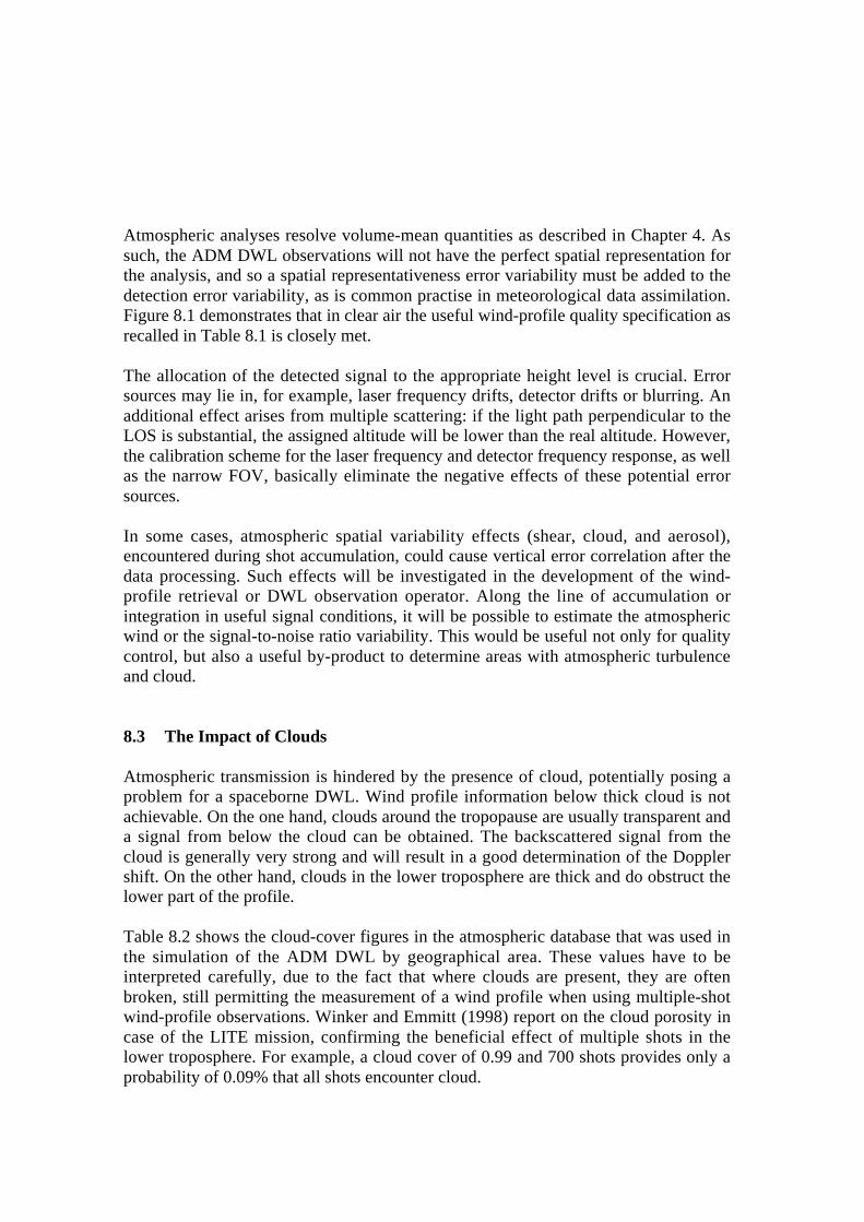
Atmospheric analyses resolve volume-mean quantities as described in Chapter 4. Assuch, the ADM DWL observations will not have the perfect spatial representation forthe analysis, and so a spatial representativeness error variability must be added to thedetection error variability, as is common practise in meteorological data assimilation.Figure 8.1 demonstrates that in clear air the useful wind-profile quality specification asrecalled in Table 8.1 is closely met.

The allocation of the detected signal to the appropriate height level is crucial. Errorsources may lie in, for example, laser frequency drifts, detector drifts or blurring. Anadditional effect arises from multiple scattering: if the light path perpendicular to theLOS is substantial, the assigned altitude will be lower than the real altitude. However,the calibration scheme for the laser frequency and detector frequency response, as wellas the narrow FOV, basically eliminate the negative effects of these potential errorsources.

In some cases, atmospheric spatial variability effects (shear, cloud, and aerosol),encountered during shot accumulation, could cause vertical error correlation after thedata processing. Such effects will be investigated in the development of the wind-profile retrieval or DWL observation operator. Along the line of accumulation orintegration in useful signal conditions, it will be possible to estimate the atmosphericwind or the signal-to-noise ratio variability. This would be useful not only for qualitycontrol, but also a useful by-product to determine areas with atmospheric turbulenceand cloud.

8.3 The Impact of Clouds

Atmospheric transmission is hindered by the presence of cloud, potentially posing aproblem for a spaceborne DWL. Wind profile information below thick cloud is notachievable. On the one hand, clouds around the tropopause are usually transparent anda signal from below the cloud can be obtained. The backscattered signal from thecloud is generally very strong and will result in a good determination of the Dopplershift. On the other hand, clouds in the lower troposphere are thick and do obstruct thelower part of the profile.

Table 8.2 shows the cloud-cover figures in the atmospheric database that was used inthe simulation of the ADM DWL by geographical area. These values have to beinterpreted carefully, due to the fact that where clouds are present, they are oftenbroken, still permitting the measurement of a wind profile when using multiple-shotwind-profile observations. Winker and Emmitt (1998) report on the cloud porosity incase of the LITE mission, confirming the beneficial effect of multiple shots in thelower troposphere. For example, a cloud cover of 0.99 and 700 shots provides only aprobability of 0.09% that all shots encounter cloud.

135

Region Polar Storm T. Subtrop. Tropics Subtrop. Storm T. Polar

Latitudes > 60S 60S-40S 40S-20S 20S-20N 20N-40N 40N-60N >60N

% Clear 37 27 32 18 40 31 34

Table 8.2. Percentage of clear-air scenes by geographical area of the atmosphericdatabase that is used in the simulation of the ADM DWL (February).

Obviously, the expected amount of energy reaching the lowest levels of thetroposphere is dependent on the total cloud cover aloft. If clear air resides below thecloud layer, a strong aerosol loading is needed to get a good-quality wind-profileretrieval using a (much) reduced number of shots. Close to the surface the aerosolloading will generally be sufficient. A cloud cover of 75% aloft will cause only aquarter of the shots to contribute to a wind observation at a particular vertical level.This leads, for the molecular return, to a decrease in the RMS accuracy of the windobservation by roughly a factor of two with respect to the clear-air performance at thatsame level.

A statistical analysis of the performance of the proposed DWL in cloudy air has beenperformed. The DWL system has been simulated in an environment where the cloudswere provided from a realistic meteorological model (Stoffelen and Marseille, 1998and 1999). Figure 8.2 depicts the signal return and wind HLOS quality as obtained inthe two cloudiest regions of the world. Below an altitude of 13 km ‘no returns’ occur,due to obstruction by thick cloud, whereas in the tropics above this level mainlytransparent clouds are present. Though few, aerosol returns occur up to 10 km height.In these regions cloud obscuration is most significant in the lower troposphere, atabout 30%. Signal quality reduction takes place in several profiles due to the presenceof cloud aloft. Cloud attenuation and obstruction are most substantial in the tropicsand in the lower troposphere in the storm track region.

A large amount of shots penetrate the lower troposphere, contributing to very goodquality winds, due to the aerosol signal detected by the Mie channel. Broken stratiformcloud in the lowest few km of the troposphere, which is quite common, may be easilypenetrated and measurements are then possible due to the strong aerosol signal closeto the Earth’s surface. The presence of cloud is most critical around the tropopauseand the cloud cover in the tropics is the most extensive according to Table 8.2. Sincehigh-level clouds tend to overlap with lower-level clouds, below the tropopause levelin the tropics cloud obstruction is relatively constant at 25%, indicating that in about75% of cases a complete profile is obtained. This would result in about 100 profilesper hour classified here as good or very good, fulfilling the requirement of Table 4.1.

The number of cloud-top-dominated returns is most important around the tropicaltropopause (35%), and less important around the storm-track region tropopause (lessthan 20%). Even though the returned Mie signal is high here, it is not clear that theobserved LOS wind is always representative of the mean flow. The cloud facet thatreturns the signal may be in a very turbulent region due to cloud dynamics. Little isknown about the detectability of strong vertical motions from a spaceborne DWL.However, vertical airborne DWL measurements over convective cloud systems seemto indicate that strong vertical cloud movements often occur below the cloud top at thetropopause, enabling good measurements to be made at the cloud top level. Furtheranalysis in this area is needed.

The proposed scheme of a smaller accumulation length within a larger integrationlength, permits the rejection of returns on dynamic clouds. In case of broken cloud themultiple accumulations in the integration area will not all have cloud-top returns, butonly a fraction of them. This fraction is close to the cloud-cover fraction when thenumber of accumulations in the integration is large, or in other words, when theaccumulation length is small compared to the integration length. By segregating thecloud-dominated and clear signals in the processing by signal-to-noise ratio, one canreduce the contamination by the cloud dynamics by applying a quality control orimproved wind retrieval (see Chapter 7). It has been demonstrated (Stoffelen andMarseille, 1998) that (for a coherent DWL concept) in about 50% of the scenes withclouds, it is still possible to retrieve winds from the clear-air return. Theirperformances were about 1.6 times worse than the requirement for clear air. However,this is still useful.

a)

137

b)

Figure 8.2. Simulated ADM DWL performances for cloudy atmospheres – The leftpanels are for the storm-track region, whereas the right ones are for the tropicalregion, i.e. both relatively cloudy regions. The top panels (a) classify the signal returnand the lower panels (b) the normalised HLOS accuracy compared with therepresentativeness error at the different vertical levels.

8.4 Usefulness for NWP

As already demonstrated with OSEs and OSSE (see Section 2.3), the impact of windprofiles on numerical weather prediction is very important. An additional aspect to beconsidered are precursor features, such as divergence or vorticity. Atmosphericstructures that are precursors to the development of extra-tropical cyclones can oftenbe identified before cyclogenesis takes place. In the preparation of the ADM, verticalwind shear has been studied as relevant example. Mid-latitude weather systems arebelieved to have their origin in processes encapsulated in the theory of baroclinicinstability. A suitable measure of the baroclinicity is provided by the Eady growth ratemaximum (e.g. Hoskins et al., 1978; Hoskins and Valdes, 1990) in which the verticalwind-shear is the main variable.

To study the impact of clouds on the detectability of vertical wind-shear, the DWLsignal return and HLOS wind quality for cases with strong wind-shear have beeninvestigated. As illustrated in figure 8.3, the signal strength and the correspondingwind quality are quite similar in the upper troposphere to cases without strong vertical

Figure 8.3. Simulated ADM DWL performances for vertical wind-shear -detectability in the storm-track region (left) and in the tropics (right). Wind-sheardetectability is only weakly correlated with the occurrence of cloud.

wind-shear, and, as such, the occurrences of shear and cloud are not very correlated(see Fig. 8.2). It has to be noted that relatively few cloud returns (very good quality)appear when strong shear is measured. Only in the lowest few km of the tropospherein the storm-track region is a reduced detectability of wind shear observed, despite theoccurrence of aerosol returns at this level. Therefore, the ADM will generally have theability to observe vertical wind-shear in broken-cloud conditions, with a possiblyslightly reduced capability close to the surface in the storm-track regions.

Beyond this, the ADM will have a major impact on wind-profile analysis. Inparticular, better wind profiles will be available in data-sparse regions like theSouthern Hemisphere or over the oceans. The ADM will not replace, but be anextremely useful complement to the existing elements of the GOS (e.g. the globalradiosonde network) by providing more frequent, more reliable and globalobservations of the wind fields in the Earth’s atmosphere.

8.5 Usefulness for Climate Studies

A proper analysis of atmospheric transport properties is fundamental for studying theEarth's climate system on several spatial and temporal scales, as outlined in Chapters 2

139

and 3. Atmospheric analyses are increasingly used to study the complex climatesystem, and re-analysis projects aim at providing consistent long-term series (ERA15,ERA40). Wind fields are important as background fields in climate models. Althoughmany aspects of the atmospheric circulation could be studied, the ADM's usefulnessfor climate studies is illustrated here mainly for humidity transport.

Important variables in the hydrological cycle and the tropical circulation are heat andhumidity transport. Stoffelen and Marseille (1998, 1999) studied the detectability oftropical fluxes of heat and humidity in cloudy areas. Obviously, processes of humiditytransport, condensation and precipitation are often associated with cloud. On the otherhand, multiple shots in case of cloud porosity (Winker and Emmitt, 1998) can enhancethe detectability of atmospheric heat and humidity fluxes in cloudy conditions asdiscussed in Section 8.2.

As an example of the usefulness of the ADM DWL for studying atmosphericprocesses associated with the energy balance, Figure 8.4 shows the quality of the windobservation in the tropics and storm-track region for those meridional moisture fluxesthat are larger than the mean plus one standard deviation of the flux variability at thelevel considered. Comparing these type of histograms with the correspondinghistograms of performance classification for all flux conditions (similar to Fig. 8.2), itcan be concluded that

• many returns from cloud appear in moist air at all geographical locations

• at altitudes in the middle and lower troposphere cloud obstruction of themoisture flux is most substantial

• for the lowest altitudes, aerosol scattering generally provides an improvedperformance in moist conditions with respect to the molecular scatteringsignal.

Thus, assuming that the horizontal line-of-sight winds observed at cloud top height arerepresentative for the general flow, a DWL in space provides essential information onthe tropical circulation in the upper troposphere. On the other hand, clouds obscure thedetectability of moisture fluxes in the middle troposphere, in particular in the tropics.Due to the Mie system, the near-surface moisture flux is well visible in the majority ofcases.

The ADM will meet the user requirements. Even in areas with high cloud cover,unfavourable for DWL wind-profiling, the ADM will provide useful information tostudy important circulation and transport properties of the atmosphere that are relevantto study our climate system, and which are outlined in Chapters 2 and 3. The missionwill provide new insights into the distribution of kinetic energy in the Earth’satmosphere.

Figure 8.4. Simulated ADM DWL performances for meridional humidity-transport -detectability in the storm-track region (left) and tropics (right) (similar to Fig. 8.2a).

8.6 Other Elements Provided by the ADM

In addition to line-of-sight velocity measurements, the ADM space-based DWL willbe able to provide information on cloud characteristics over the depth of theatmosphere, as well as aerosol measurements in the troposphere. These include:

• cloud top height (notably cirrus top and base)

• cloud cover

• cloud and aerosol extinction and optical thickness

• identification of multi-layer clouds

• a measure of clear-air turbulence or other wind variability

• lower-troposphere aerosol stratification

• the height of the tropopause

• the height of the planetary boundary layer (PBL).

The properties of these secondary products are determined by the requirements for thewind-profile product. The vertical resolution of the secondary products is the same asthe one used for the velocity measurements. The horizontal resolution of theinformation is locally enhanced, depending on the shot-accumulation strategy. Sincepriority has been given to the LOS wind measurement, only a small effort has so far

141

been put into the retrieval of the secondary products, so that the above list needs to befurther explored.

Cloud properties are prognostic variables in some atmospheric models now and willbe even more so in the future. In a four-dimensional data-assimilation scheme, someof the DWL cloud products may be assimilated directly in the atmospheric analysis.The cloud information is relevant for radiative-transfer calculations in the model.Tropopause and PBL height may also be validated against forecast and generalcirculation models. Moreover, DWL cloud top winds are a unique validation ofgeostationary cloud-motion winds. Many atmospheric circulation models currently usea fixed aerosol profile. The tropospheric aerosol products may be inserted as tracers inthe data-assimilation system, again to benefit radiative-transfer calculations, but alsochemistry computations. This in turn may be helpful for the ADM data processing.

8.7 Conclusions

The ADM will meet the scientific objectives outlined in Chapters 2 and 3. It will meetthe observational requirements tabled in Chapter 4. The ultraviolet concept presentedin Chapter 6 has the potential to meet the ideal user requirements (as tabled inSection 4.1) which will provide an increased beneficial impact from spaceborne windprofile measurements in atmospheric analyses, modelling, and prediction. Theproposed demonstration ADM will pave the way to future operational wind-profilingmissions.

The expected accuracy of the measured DWL HLOS winds in clear air is very similarto conventional meteorological wind-profile observations. However, the DWL windprofiles result in a much more uniform sampling over the globe. They cover theoceans with a density similar to the mean density of the ground-based wind profilesover land in the Northern Hemisphere.

As shown in Chapter 2, although distributed very irregularly, the conventional wind-profiling network is of key importance to atmospheric analyses and weather forecasts.The proposed wind-profiling complement is, therefore, expected to be very beneficial.

The impact of cloud on the DWL performance is very important. Although lidarsignals are able to penetrate thin clouds (e.g. cirrus) to a certain extent, opaque cloudsobscure the underlying atmosphere. It is shown that multiple shots are a good strategyfor deeper atmospheric penetration in case of broken cloud. As such, the DWLprovides good detectability of the near-surface moisture flux due to aerosol detection,which is important for climate studies. The impact of multiple shots is most substantialin the tropics.

The improved analyses will be of benefit for both tropical and extra-tropical weatherforecasts. Improved information on transport and circulation will be beneficial for

climate studies as detailed in Chapter 2. In particular, improved advection of tracers,like ozone, aerosol, or other species, would benefit the atmospheric-chemistrycommunity, and enable enhanced analysis of humidity convergence.

The Atmospheric Dynamics Mission will make a unique contribution to atmosphericmodelling and research by providing, for the first time, one of the key parameters , i.e.the atmospheric wind, directly and globally. The mission is therefore a trueexploratory mission.

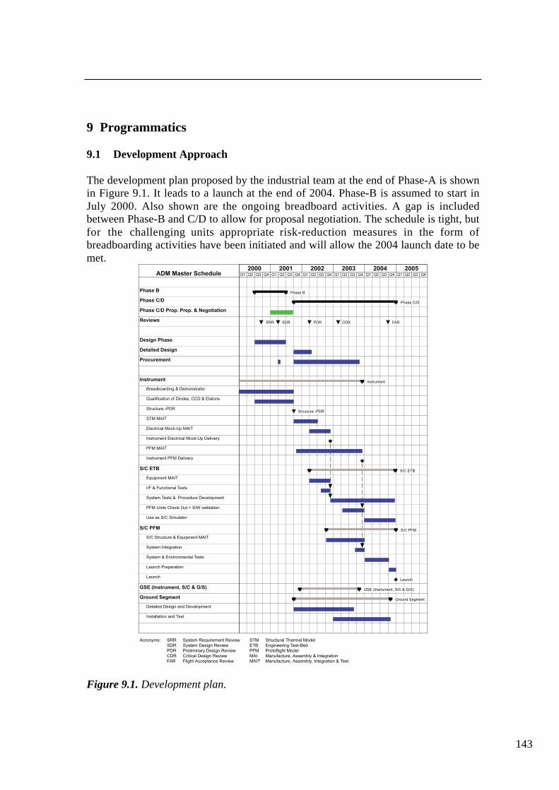
143

9 Programmatics

9.1 Development Approach

The development plan proposed by the industrial team at the end of Phase-A is shownin Figure 9.1. It leads to a launch at the end of 2004. Phase-B is assumed to start inJuly 2000. Also shown are the ongoing breadboard activities. A gap is includedbetween Phase-B and C/D to allow for proposal negotiation. The schedule is tight, butfor the challenging units appropriate risk-reduction measures in the form of breadboarding activities have been initiated and will allow the 2004 launch date to bemet.

! " " # ! $ %&# ' # ! $ %$# &

%&

(!! $""&

#

)*'#

# )*'

#

#

!"

' #

#+ &

& '

*" ),-+.

* +"

#

+" &' #

#

&

/ '

/

$!% &$'

$

'

#

"+

"

#

+"

+"

/

01# $+"&0+2

0

(3 (4 (5 (6 (3 (4 (5 (6 (3 (4 (5 (6 (3 (4 (5 (6 (3 (4 (5 (6 (3 (4 (5 (6())) ())* ())( ())+ ()), ())-

Figure 9.1. Development plan.

The model philosophy and the development flow are shown in Figure 9.2. Adistinction is made between the instrument and the platform equipment. For theinstrument, a structural-thermal model (STM) is proposed consisting of the opto-mechanical and thermal subsystem and dummies of the other elements. For thetransmitter and receiver subsystems, it is proposed to build-up breadboards, atqualification-model level for key elements. Subsequently, this breadboard will becompleted on an EM level to an electrical mock-up used for electrical and functionaltesting at instrument level. For interface and functional system tests, this mock-up willthen be connected to an engineering test bed (ETB).

Concerning the spacecraft equipment, engineering/qualification models are proposedto perform delta qualifications for the power control and distribution unit (PCDU) andthe CDMS described in Section 6.5.3. For these units, qualified designs already existat board level and therefore structural and thermal qualification will be done withproto-flight models. Only flight models are procured for all other platform units. Thespacecraft is also functionally tested in the ETB.

Engineering Test-Bed

(ETB)

PFMAcceptance or Protoflight Testing

Electrical and Functional Testing

Protoflight Testing

I/F, Electricaland Functional

Testing

S/C Equipment

System

STM

PFM

FM or PFM

EM or FM

Structural & Thermal Qualification

Protoflight Testing

Instrument

ElectricalMock-up

Electrical and Functional Testing

S/C StructureDesign Validation by Analysis

Spares

Launch

145

9.2 Heritage, Critical Areas and Risks

Table 9.1 shows the implementation and heritage for the ADM space and groundsegment. The large heritage at platform level and the pre-development activities forthe instrument are to be noted.

Implementation Heritage

ALADIN InstrumentConcept Frequency tripled Nd:YAG,

130 mJ 100 HzMediumPowerOscillator

Q-switched diode pumped Nd:YAG130 mJ @1.06 µm

Based on existing ground based militaryapplication designs

PowerAmplifier

Diode pumped Nd:YAG350-400 mJ @ 1.06µm

Based on existing ground based militaryapplication designs

FrequencyTripler

KD*P or LBO nonlinear crystals,efficiency >30%

Efficiencies demonstrated in variousapplications, dedicated test programconducted in Phase-A

Q-Switch KD*P design with dedicated highvoltage electronics

Identical unit developed and successfullytested in frame of ATLID breadboardingactivities

Pump Diodes 1 kW stack or autostack diodes Commercial products from Europeansuppliers; life test data available

Pump DiodeElectronics

Current pulses of 150 µs with 85 Aat 192 V

Representative BB developed andsuccessfully tested in frame of ATLID

Referenceand SeedLaser withDriveElectronics

Low power CW diode pumped non-planar ring lasers

Available as commercial product fromEuropean supplier

Transmitter

ThermalControl

Heat pipe Standard space product

RayleighReceiver

Double edge Fabry Perot Already manufactured and tested byService d´Aéronomie-CNRS; spacequalified technologies are used

Mie Receiver Fizeau interferometer A B/B is already manufactured andtested (IDWL study). Space qualifiedtechnologies are used (molecularbonding)

Detector Thinned back illuminated CCD inaccumulation mode

All technologies are validated onGOMOS spectrometer. Performance andoperation concept will be validated onprototype to be tested before end of 1999

Filters Interference and Fabry Perot filters Based on existing designs

Receiver

DetectionChainArchitectureandOperation

Partly validated during IDWL

Telescope PrimaryMirror andStructure

1.1m diameterF/0.9 apertureAll SiC design

Derived from FIRST and OSIRISdevelopment activities

Core Instrument Structure All SiC design FIRST, OSIRIS structural and flightmodels, early breadboarding

Implementation Heritage

Platform

Configuration Integrated satellite design directlyserving required instrumentaccommodation

Offered by most LEO spacecrafts,e.g. Flexbus, Leostar, Proteus, etc..

Structure Box type structure with central conebased on aluminium honeycombelements

Very large heritage in numerous ESAprogrammes by use of standard materialand technology

Thermal Conventional passive design withheat pipes, heaters, radiators,thermistors, ...

Very large heritage in numerous ESAEO and science missions

Attitude 3-axis controlled off-nadir acrosstrack pointing with yaw steering

Can directly be implemented by mostLEO platforms

Sensors Star tracker, 3-axis magnetometer,inertial reference unit (IRU)

Off-the shelf equipment

Actuators 4 ball bearing reaction wheels + 3magnetotorquers

Off-the shelf equipment

Positioning GPS receiver equipment Off-the shelf equipment

AOCS

Propulsion 4 x 1N Hydrazine thrusters and100 kg fuel and tank

Off-the shelf equipment

Concept Integrated data management system Heritage from small satellites e.g.Leostar, Flexbus, Proteus

Data Bus IEEE 1355 for intelligent users, RS422/485 for non-intelligent users

Standard, parts are available

Computer Data management based on singleplatform computer, centralisedavionics S/W for satellite command& control, AOCS, thermal, etc

Based on ERC 32 processordevelopment

Data Handling

Data Storage 256 Mbit memory unit Reuse of already existing design, e.g.Cluster

TT&C Standard S-Band transponder, 2 kbpsuplink, 64 kbps downlink

Off-the shelf equipmentComm’s

Payload DataTransmission

Instrument data downlink viameteorological L-Band with3.5 Mbps

Reuse of existing hardware as presentlyin development for Metop

Solar Array 8.4 m2 in 2 fixed wings,based on Si-BFSR cells

Reuse of Globalstar design,several potential suppliers for cells

Battery NiCd battery with 18 Ah Off-the shelf equipment

Power

Regulation Hybrid power bus design,unregulated for instrument, regulatedfor all other

Large heritage for both, regulated andunregulated bus technology

Launcher Rockot SS19, Breeze on Proton,two demo flights in 1999

147

Ground Segment

CDAE Data dump every orbit required,hence two near-polar L-band stationsnecessary

L-band receiving station already indevelopment for METOP groundsegment

MSCE Standard mission operations andcontrol

Large heritage, e.g. at ESOC

GroundSegmentElements

PAE Data processing and archiving up toLevel 1, data distribution to ScienceData Processing Centre

Large heritage, e.g. at Eumetsat

Table 9.1. Implementation and heritage.

Table 9.2 shows the critical areas identified at the end of Phase-A and the proposedrisk-reduction measures. Critical areas concern only the instrument, where criticality islow to moderate. The key elements exist already, which allows us to be confidentregarding the technology. It is necessary, however, to verify the end-to-endperformance of all elements integrated and to demonstrate the flight compatibility.This is achieved by proposing early breadboard and qualification activities, partiallystarted already, and establishing the appropriate model philosophy as defined inSection 9.1.

Critical Areas Risk ReductionALADIN Instrument

Lasers End–to-end performance in terms ofpulse energy, beam profile andqualification

Dedicated transmitter BB initiatedTransmitter

PumpDiodes

Formal space qualification Dedicated lifetime verificationprogramme initiated

CCD Charge transfer efficiency Dedicated test programme initiatedReceiverCombinedMie andRayleighReceiver

Proper function of combined receiver Performance verification in frame ofIDWL running.

Table 9.2. Critical areas and risk-reduction measures.

No critical areas have been identified in the platform and the ground segment. For thelauncher, there are alternatives to Rockot.

In summary, the proposed implementation concept has a few areas of low to moderatecriticality at instrument level, related more to ‘putting together’ elements than totechnological challenges.

9.3 Related Missions, International Co-operation Possibilities and Timeliness

The NPOESS lists wind profiles as a top priority observation which, however, is notcovered by the present NPOESS baseline. In view of the high interest, mission

concepts are being mentioned in the USA (and also in Japan), but no consolidatedplans exist at this time. SPARCLE is a NASA experiment consisting of flying a 2micron system on the Space Shuttle. It is planned for launch in 2001 and to last for thetypical duration of a Shuttle flight. It will provide data only for the lowest km of theatmosphere.

Co-operation can be envisaged within Europe with other European internationalorganisations. Eumetsat have shown their interest in the ADM and could participate,e.g. facilitating the archiving and the near-real-time data distribution to operationalusers. The ECWMF has indicated an interest in becoming the lead centre inassimilating ADM data.

Co-operation could also be sought with NASA / NOAA and consist, as a minimum, ofthe provision of a high-latitude data-acquisition station, e.g. Barrows in Alaska, toguarantee near-real-time data provision for all orbits.

The ADM is very timely. It will allow to develop all capabilities scientific, technical,technological and operational in time for deployment in a future operational system ofthe Joint Polar System that includes the American NPOESS and the Eumetsat PolarSystem (EPS) with the METOP satellites.

9.4 Enhancement of Capabilities and Applications Potential

The expected advances in science have been discussed in previous chapters. Thismission is also very relevant to the enhancement of capabilities to enable applicationsand future operational systems.

The potential for operational application of the ADM observations has beenrecognised for many years and recalled again recently (WMO,1998). Eumetsat and themeteorological services have also shown an interest in the operational utilisation ofwind-profile observations.

The ADM will develop the underlying science, the technology, the observationtechniques, the models and the assimilation schemes and operational practicesrequired to provide these applications with operational systems on a routine basis. TheADM science and technology developments will provide almost immediate returns.The need for and usefulness of the ADM are clearly apparent.

The ADM will allow Europe to develop its position in space lasers, a domain inwhich, despite the investments for more than a decade, the lack of a mission preventsit from being present in this critical technological area.

149

References

Atlas, R., 1998: Potential impact of a DWL on weather analyses and forecasts, Zephyrproject presentation, http://zephyr1.gsfc.nasa.gov.

Cardinali, C., J. Pailleux and J.N. Thépaut, 1998: Use of simulated satellite dopplerwind lidar data in NWP: an impact study, CNRM/GMAP Note No. 6.

Chanin, M.L. et al., 1994: Recent lidar developments to monitor stratosphere-troposphere exchange, J. Atmos. Terr. Phys., 56, 1073-1081.

Courtier, P., P. Gauthier and F. Rabier, 1992: Study of preparation for the use ofDoppler wind lidar information in meteorological assimilation systems; ESA-CR(P)-3453.

Cress, A.,1999: Impact of wind profile observations on the German Weather Service'sNWP system, Arbeitsergebnisse Nr. 56, Geschäftsbereich Forschung undEntwicklung, DWD, Offenbach. ISSN 1430-0281.

European Space Agency, 1996: Atmospheric Dynamics Mission, ESA SP-1196 (4).

European Space Agency, 1998: The Science and Research Elements of ESA’s LivingPlanet Programme, ESA SP-1227, 105p.

Flesia, C., and C.L. Korb, 1999: Theory of the Double-edge molecular technique forDoppler Lidar wind measurement, Appl. Opt., 38, 432-440.

Garnier, A., and M.L. Chanin, , 1992: Description of a Doppler Rayleigh lidar formeasuring winds in the middle atmosphere, Appl. Phys., B55, 35-40.

Hello, G., F. Lalaurette and J. N. Thépaut, 1999: Combined use of sensitivityinformation and observations to improve meteorological forecasts: the “Christmasstorm” case, Accepted in Quart. J. Roy. Meteor. Soc.

Hollingsworth, A. and P. Lönnberg, 1987: The statistical structure of short-rangeforecast errors as determined from radiosonde data. Part I: The wind field. Part II: Thecovariance of height and wind error, Tellus, 38A, 111-136 and 137-161.

Hoskins, B. J., and P. J. Valdes, 1990: On the existence of storm tracks, J. Atmos. Sci.47, 1854-1864.

Hoskins, B. J., I. Draghici, and H. C. Davies, 1978: A new look at the ω-equation,Quart. J. Roy. Meteor. Soc., 104, 31-38.

Ingmann, P., L. Isaksen, A. Stoffelen and G.-J. Marseille, 1999: On the Needs,Requirements and Feasibility of a Space-borne Wind Profiler, Proc. of ‘FourthInternational Winds Workshop’, Eumetsat, EUM P 24, 199-206.

Kållberg, P., and S. Uppala, 1999: Impact of Cloud Motion Winds in the ECMWFERA15 Reanalysis, Proc. of ‘Fourth International Winds Workshop’, Eumetsat, EUMP 24, 109-116.

Kelly, G.A., 1997: Influence of observations on the Operational ECMWF System,WMO Bulletin, 46, 336-342.

Kelly, G.A., M. Tomassini and M. Matricardi, 1996: Meteosat cloud-cleared radiancesfor use in three/four dimensional variational data assimilation, Proc. ‘ThirdInternational Winds Workshop’, Eumetsat, EUM P 18, 105-116.

Lorenc, A.C., 1986: Analysis methods for numerical weather prediction, Quart. J.Roy. Meteor. Soc, 112, 1177-1194.

Lorenc, A.C., R.J. Graham, I. Dharssi, B. Macpherson, N.B. Ingleby andR.W. Lunnon, 1992: Preparation for the use of Doppler wind lidar information inmeteorological assimilation systems; ESA-CR(P)-3454.

McNally, A.P. and M. Vesperini, 1995: Variational analysis of humidity informationfrom TOVS radiometer, Eumetsat/ECMWF Fellowship Programme, Research ReportNo. 1, ECMWF.

Meteorological Society of Japan, 1997: Special issue of the Journal of theMeteorological Society of Japan documenting the symposium on data assimilation inmeteorology and oceanography (Tokyo - 13-17 March 1997). J. Meteor. Soc. Japan,75, No 1B, 111-496.

Peuch, A., J.N. Thépaut and J. Pailleux, 1999: An OSSE using TOVS total ozone data.Proc. ’SODA Workshop on Chemical Data Assimilation’, KNMI TR-189.

Rabier, F., J.N. Thépaut and P. Courtier, 1998a: Extended assimilation and forecastexperiments with a four-dimensional variational assimilation system, Quart. J. Roy.Meteor. Soc., 124, 1861-1887.

Rabier, F., A. McNally, E. Anderson, P. Courtier, P. Unden, J. Eyre, A. Hollingsworthand F. Bouttier, 1998b: The ECMWF implementation of three-dimensional variationalassimilation (3D-Var). II: Structure functions. Quart. J. Roy. Meteor. Soc, 124, 1809-1829.

151

Räisänen, J., 1998: CMIP2 subproject climate change in northern Europe - Plans andfirst results. Proceedings of ‘CMIP Project Workshop’, Melbourne, Australia, 14-15October, 1998.

Rees, D. et al., 1996: The Doppler wind and temperature system of the ALOMARlidar, J. Atmos. Terr. Phys., 58, 1827-1842.

Stoffelen, A., 1998: Scatterometry, Thesis Utrecht University, ISBN 90-393-1708-9.

Stoffelen, A. and G.J. Marseille, 1998: Study on the utility of doppler wind lidar datafor numerical weather prediction and climate, ESA CR(P)-4198.

Stoffelen, A., and G.J. Marseille, 1999: Performance analysis of a DWL for the ADM,Project report for LIPAS, ESA Contract No. 3-9132/97.

Stoffelen, A. and H. Eskes (Eds.), 1999: Proceedings of SODA Workshop onChemical Data Assimilation, KNMI TR-189.

Vaughan, M. and D. Willetts, 1998: Influence of atmospheric turbulence, shear,aerosols stratification and cloud motion on space Doppler wind lidar signals, ESTECContract No. 12006/96/NL/CN.

Vaughan, M., P. Flamant and C. Flesia, 1999: Scientific concept trade-off, ESAContract No. 12510/97/NL/RE.

Winker, G.D. and D.M. Emmitt, 1998: Relevance of cloud statistics derived fromLITE data to future Doppler wind lidars, Proc. ‘9th Conference on Coherent LaserRadar’, 23-27 June 1997. Linköping, Sweden, p 144-147.

World Meteorological Organisation 1995: Plan for the Global Climate ObservingSystem (GCOS), Version 1, WMO/TD-No. 681.

World Meteorological Organisation, 1996: Guide to Meteorological Instruments andMethods of Observation, 6th edition, WMO-No.8, Secretariat of the WorldMeteorological Organisation, Geneva, Switzerland.

World Meteorological Organisation, 1997: Impact of various observing systems onnumerical weather prediction. Proceedings of the ‘CGC/WMO Workshop’ held inGeneva, 7-9 April 1997 (Ed.: J. Pailleux). WWW Technical Report No 18. WMO/TDNo. 868.

World Meteorological Organisation, 1998: Preliminary Statement of GuidanceRegarding How Well Satellite Capabilities Meet WMO User Requirements in SeveralApplication Areas. WMO Satellite Reports SAT-21. WMO/TD No 913.

153

Glossary

ADM Atmospheric Dynamics MissionADMAG ADM Advisory GroupADM-FF ADM Free FlyerAIREP WMO Code for Aircraft ReportAIU AOCS Interface UnitALADIN Atmospheric Laser Doppler InstrumentAOCS Attitude and Orbit Control SystemARPEGE Action de Recherche Petite Echelle Grande Echelle (French

climate model)ASH Acquisition and Safe HoldATLID Atmospheric LidarATOVS Advanced TOVSCCD Charged-coupled DeviceCDAE Command and Data Acquisition ElementCDMS Control and Data Management SystemCDR Critical Design ReviewCEOS Committee on Earth Observing SatellitesCFRP Carbon Fibre Reinforced PlasticCLIVAR Programme on Climate VariabilityCMW Cloud Motion WindCOG Centre of GravityCW Continuous WaveDE Double EdgeDOD Depth of DischargeDWD Deutscher WetterdienstDWL Doppler Wind LidarECMWF European Centre for Medium-range Weather ForecastsEM Engineering ModelEMC Electro-magnetic CompatibilityENSO El Niño Southern OscillationEPS Electrical Power Sub-systemERA ECMWF Re-analysisERS European Remote-sensing SatelliteESA European Space AgencyESOC European Space Operations CentreETB Engineering Test-bedFAR Flight Acceptance ReviewFIRST Far-infared Space TelescopeFM Flight ModelFOV Field-of-ViewFWHM Full-Width Half-MaximumGCOS Global Climate Observing System

GEWEX Global Energy and Water Cycle ExperimentGMT Greenwich Mean TimeGNSS Global Navigation Satellite SystemGOS Global Observing SystemGPS Global Positioning SystemHLOS Horizontal LOSHRPT High Resolution Picture TransmissionIASI Infrared Atmospheric Sounding InterferometerISS International Space StationITCZ Inter-Tropical Convergence ZoneLEOP Launch and Early Orbit PhaseLIDAR Light Detection and RangingLITE Lidar-In-space Technology ExperimentLOS Line of SightLTAN Local Time of Ascending NoteMAI Manufacture, Assembly and IntegrationMAIT MAI and TestMC Multi-ChannelMETOP Future European meteorological polar-orbiting satelliteMLI Multi-Level InsulationMMS Matra Marconi SpaceMOSFET Metal Oxide Semiconductor Field Effect TransistorMSCE Mission Operations and Satellite Control ElementMSLP Mean Sea Level PressureNCEP National Center for Environmental Prediction (USA)NH Northern HemisphereNOAA National Oceanic and Atmospheric AdministrationNWP Numerical Weather PredictionOBDH On-board Data Handling systemORATOS Orbit Attitude Operations SystemOSE Observation System ExperimentOSSE Observation System Simulation ExperimentPAE Processing and Archiving ElementPBL Planetary Boundary LayerPCDU Power Control and Distribution UnitPDF Probability Density FunctionPDR Preliminary Design ReviewPDT Payload Data TransmissionPDTS PDT Sub-systemPFM Protoflight ModelPILOT WMO Code for Conventional Wind SoundingPLH Power Laser HeadPLL Phase Locked LoopPRF Pulse Repetition FrequencyQC Quality Control

155

RCS Reaction Control SystemRFDU Radio Frequency Distribution UnitRMS Root Mean SquareRockot Russian LauncherRTU Remote Terminal UnitSATOB WMO Code for CMW Satellite ObservationS/C SpacecraftSCOS Satellite Control Operating SystemSDPC Science Data Processing CentreSDR System Design ReviewSH Southern HemisphereSNR Signal-to-Noise RatioSOIRD S/C Operations Interface Requirements DocumentSRR System Requirement ReviewSSM/I Special Sensor Microwave / ImagerSSMM Solid-State Mass MemorySSPA Solid-State Power AmplifierSTM Structural Thermal ModelTC/TM Telecommand and TelemetryTEMP WMO Code for Conventional Wind, Temperature and Humidity

SoundingTOGA Tropical Ocean and Global AtmosphereTOMS Total Ozone Monitoring SpectrometerTOVS TIROS-N Operational Vertical SounderTT&C Telemetry, Tracking and CommandUARS Upper Atmosphere Research SatelliteUKMO United Kingdom Meteorological OfficeUTC Universal Time CoordinatedUV Ultra-VioletWCRP World Climate Research ProgrammeWGS World Geodetic SystemWMO World Meteorological OrganisationWWB Westerly Wind BurstWWE Westerly Wind EventsWWW World Weather Watch4D-Var Four-dimensional Variational Assimilation

157

Acknowledgements

We are very grateful for the valuable contributions from A. Culoma, U. Kummer andR. Meynart.

Thanks are also extended to C. Readings, M.L. Reynolds and A. Tobias for their timeand effort in reviewing the document, and to D. Reinprecht for preparing thedocument for publication.