atmospheric boundary layer top height in south africa ... · atmospheric boundary layer top height...

Atmos. Chem. Phys., 14, 4263–4278, 2014www.atmos-chem-phys.net/14/4263/2014/doi:10.5194/acp-14-4263-2014© Author(s) 2014. CC Attribution 3.0 License.

Atmospheric Chemistry

and PhysicsO

pen Access

Atmospheric boundary layer top height in South Africa:measurements with lidar and radiosonde compared to threeatmospheric models

K. Korhonen1,2, E. Giannakaki1, T. Mielonen1, A. Pfüller1, L. Laakso3,4, V. Vakkari 3,5, H. Baars6, R. Engelmann6, J.P. Beukes4, P. G. Van Zyl4, A. Ramandh7, L. Ntsangwane8, M. Josipovic4, P. Tiitta2,4,9, G. Fourie7, I. Ngwana8,K. Chiloane10, and M. Komppula1

1Finnish Meteorological Institute, P.O. Box 1627, 70211, Kuopio, Finland2Department of Applied Physics, University of Eastern Finland, P.O. Box 1627, 70211 Kuopio, Finland3Finnish Meteorological Institute, P.O. Box 503, 00101, Helsinki, Finland4Unit for Environmental Sciences and Management, North-West University, Potchefstroom, South Africa5Department of Physics, University of Helsinki, P.O. Box 64, 00014 Helsinki, Finland6Leibniz Institute for Tropospheric Research, Permoserstrasse 15, 04318, Leipzig, Germany7Sasol Technology R&D (Pty) Ltd., P.O. Box 1, Sasolburg, South Africa8South African Weather Service, Pretoria, South Africa9Department of Environmental Sciences, University of Eastern Finland, P.O. Box 1627, 70211 Kuopio, Finland10Eskom Holdings SOC Ltd; Sustainability Division; Research, Testing and Development, South Africa

Correspondence to:M. Komppula ([email protected])

Received: 16 April 2013 – Published in Atmos. Chem. Phys. Discuss.: 1 July 2013Revised: 15 March 2014 – Accepted: 17 March 2014 – Published: 30 April 2014

Abstract. Atmospheric lidar measurements were carried outat Elandsfontein measurement station, on the eastern High-veld approximately 150 km east of Johannesburg in SouthAfrica throughout 2010. The height of the planetary bound-ary layer (PBL) top was continuously measured using a Ra-man lidar, PollyXT (POrtabLe L idar sYstem eXTended).High atmospheric variability together with a large surfacetemperature range and significant seasonal changes in pre-cipitation were observed, which had an impact on the verti-cal mixing of particulate matter, and hence, on the PBL evo-lution. The results were compared to radiosondes, CALIOP(Cloud-Aerosol Lidar with Orthogonal Polarization) space-borne lidar measurements and three atmospheric models thatfollowed different approaches to determine the PBL topheight. These models included two weather forecast mod-els operated by ECMWF (European Centre for Medium-range Weather Forecasts) and SAWS (South African WeatherService), and one mesoscale prognostic meteorological andair pollution regulatory model TAPM (The Air PollutionModel). The ground-based lidar used in this study was oper-

ational for 4935 h during 2010 (49 % of the time). The PBLtop height was detected 86 % of the total measurement time(42 % of the total time). Large seasonal and diurnal varia-tions were observed between the different methods utilised.High variation was found when lidar measurements werecompared to radiosonde measurements. This could be par-tially due to the distance between the lidar measurementsand the radiosondes, which were 120 km apart. Compari-son of lidar measurements to the models indicated that theECMWF model agreed the best with mean relative differ-ence of 15.4 %, while the second best correlation was withthe SAWS model with corresponding difference of 20.1 %.TAPM was found to have a tendency to underestimate thePBL top height. The wind speeds in the SAWS and TAPMmodels were strongly underestimated which probably led tounderestimation of the vertical wind and turbulence and thusunderestimation of the PBL top height. Comparison betweenground-based and satellite lidar shows good agreement witha correlation coefficient of 0.88. On average, the daily max-imum PBL top height in October (spring) and June (winter)

Published by Copernicus Publications on behalf of the European Geosciences Union.

4264 K. Korhonen et al.: Atmospheric boundary layer top height in South Africa

was 2260 m and 1480 m, respectively. To our knowledge, thisstudy is the first long-term study of PBL top heights and PBLgrowth rates in South Africa.

1 Introduction

The planetary boundary layer (PBL), being the lowest part ofthe atmosphere, is strongly affected by the Earth’s surface atall times of the day. Daily PBL development is conditionedby several parameters such as local thermal and dynamicforcings, as well as by forcing on a synoptic scale. The vari-ance in local forcings (e.g. surface temperature) causes spa-tial and temporal alteration in PBL dynamics. For instance,ground-based emissions of particulate matter are mixed anddistributed mainly inside the PBL.

Seibert et al. (2000) published a comprehensive study onthe comparison of different operative measurement methodsfor PBL top height, where the importance of choosing be-tween acknowledged definitions of PBL is emphasised. Weadopted the definition used by Stull (1988), according towhich the PBL top is defined as the lowest part of the tro-posphere that is directly influenced by the earth’s surface,which responds to surface forcings within one hour or less.

There are many methods for determining the PBL heightfrom vertically resolved measurements. Globally, measure-ment with radiosondes is a widely applied operationalmethod (Seibert et al., 2000). Quality-controlled radiosondedata has been available for decades, which makes the methodsuitable for long-term climatological studies on many conti-nents (Seidel et al., 2012). There have been numerous stud-ies on the determination of the PBL height from radiosondemeasurement data (e.g. Johansson and Bergström, 2005) andit is known that the interpretation is not always straightfor-ward due to technical limitations (van Pul et al., 1994), suchas altering vertical resolution due to horizontal movementalong wind fields during the ascent of the instrument.

PBL top height is a crucial component in air pollutionmodels because it determines the vertical space and conse-quently the volume for pollutant mixing, which is a key pa-rameter for assessment of concentrations. Turbulence in airflow due to surface friction also affects the horizontal dis-tribution of pollutants and is an important factor in weatherforecast models. The PBL height cannot be directly mea-sured by standard meteorological observations but it is aquantity that can be derived from the observations. The dif-ferent parametrisations of models affect the precision of thesimulated PBL height and therefore validation with measure-ments is essential (e.g. Hurley et al., 2008).

Lidar (light detection and ranging) systems provide con-tinuous measurement of numerous atmospheric quantities,including the vertical profile of atmospheric aerosols fromwhich the PBL height can be derived (Matthias et al., 2004;Amiridis et al., 2007; Baars et al., 2008; Groß et al., 2011;

Tsaknakis et al., 2011; Haeffelin et al., 2012; Cimini et al.,2013). Aerosols and pollutants are vertically mixed inside thePBL during daytime when mixing is driven by convectionand turbulence in air flow. The PBL top height is indicatedby a gradient in the vertical backscatter coefficient profilederived from the lidar measurement signal.

PBL top height determination is also possible using datafrom an active space-borne lidar, which possesses the abilityto view vast and remote areas on a regular basis. Attenuatedbackscatter profiles derived from the measurements of theCALIOP (Cloud-Aerosol Lidar with Orthogonal Polariza-tion) on board the CALIPSO (Cloud-Aerosol Lidar and In-frared Pathfinder Satellite Observations, Winker et al., 2004,2006, 2007) satellite can be used to study the vertical struc-ture of aerosols, and hence, to define the PBL top height (Jor-dan et al., 2010). However, operational CALIOP PBL prod-uct is currently not available.

Previous studies have indicated that South Africa is oneof the most affected countries with regard to aerosol load,due to various natural and anthropogenic activities (Piketh etal., 1999, 2002; Formenti et al., 2002, 2003; Liu, 2005; Que-face et al., 2011). In addition to information already derivedfrom the above-mentioned studies, lidar studies can give de-tailed information on the vertical stratification, optical andmicrophysical properties of aerosols. A detailed character-isation of aerosol properties, vertical stratification, mixing,and aging behaviour of aerosols in West Africa has beenperformed based on a unique data set of spectrally resolvedbackscatter and extinction coefficients and the depolarisa-tion ratio (Ansmann et al., 2009, 2011). The authors stud-ied the complex layer structure of Sahara dust and biomassburning aerosols observed at Praia, Cape Verde and how theAfrican plume reached the South American coast. Campbellet al. (2003) have found lidar ratios between 50 and 90 sr,with the Ångström exponent of 1.5–2, for dense biomasssmoke events during the South African Regional Science Ini-tiative (SAFARI) 2000 (Swap et al., 2003). The lidar ratio(Ansmann et al., 1992) and Ångström exponent (Ångström,1929) refer to the extinction-to-backscatter ratio and wave-length dependency of aerosol extinction or backscatter coef-ficient, respectively.They studied backscatter profiles from amicropulse lidar system and compared the results to Sun pho-tometer aerosol optical depth measurements. As these exam-ples indicate, lidar studies in South Africa have mostly beenlimited to specific case studies.

In this study we conducted continuous long-term ground-based lidar measurements at Elandsfontein, South Africa,throughout the year 2010 in the framework of the EUCAARI(European Integrated Project on Aerosol Cloud Climate andAir Quality Interactions) project (Kulmala et al., 2011). Thisis a relatively polluted region where the number of previousatmospheric measurement campaigns has been limited. Wecompared one year of PBL top height data retrieved from aground-based lidar measurements with radiosondes, three at-mospheric models and space-borne lidar retrievals. The aim

Atmos. Chem. Phys., 14, 4263–4278, 2014 www.atmos-chem-phys.net/14/4263/2014/

K. Korhonen et al.: Atmospheric boundary layer top height in South Africa 4265

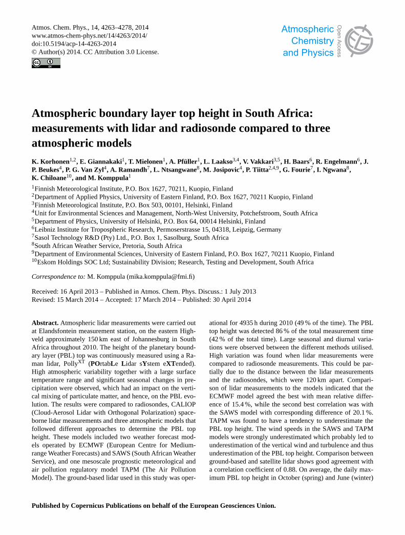
Fig. 1. Location of measurement site and the orographic information of the surroundings. The Elandsfontein lidar site was located 150 kmeast from Johannesburg. The map shows the location of the Pretoria sounding station 120 km from the lidar site.

of this study was to provide information on PBL characteris-tics in South Africa, and to compare the measured PBL topheights to ones simulated by different atmospheric models.This study is the first long-term study of PBL top heightsand PBL growth rates in South Africa.

2 The measurement site

The lidar measurement site was located on a hill top atElandsfontein (26◦15′ S, 29◦26′ E, 1745 m a.s.l, which is sit-uated in the eastern part of the Highveld region (Fig. 1) inSouth Africa. The Highveld is a large plateau that covers400 000 km2, with an average mean altitude of 1500 m a.s.l,varying from 1400 up to 1800 m a.s.l. (Fig. 1). The localtime zone is UTC+2 and it has been used in the presenta-tion of all data. The station is located about 150 km east fromthe Johannesburg–Pretoria megacity, the largest metropoli-tan area in South Africa with a population of over 10 millionpeople (Lourens et al., 2012). The surroundings close to theElandsfontein site are mostly rural with agriculture activities,while the larger region includes mining and industrial activ-ities. Laakso et al. (2012) gave a detailed description of themeasurement site.

The main anthropogenic emission sources in this area in-clude high-capacity power production with coal-fired powerplants (Lourens et al., 2011), yielding nearly half of all elec-tricity produced on the African continent. In addition, thereare many other industrial sources of nitrogen and sulfuricoxides, such as petrochemical industry and mining activi-ties. The area surrounding the measurement site is globallyregarded as one of the top five hotspots of nitrogen oxideemissions (Lourens et al., 2011, 2012). Other anthropogenicemissions in this area include household combustion (forspace heating and cooking) and controlled, as well as uncon-trolled burning of vegetation. Wildfires and controlled burn-

ing of vegetation are significant sources of particulate emis-sions, especially during May–September. During the mea-surement campaign the fire frequency in the surroundingsof Elandsfontein was highest in September (the end of thedry season), and lowest in March (the end of the wet season)(http://earthdata.nasa.gov/data/near-real-time-data/firms).

A dominant characteristic of the South African Highveldclimate is the variation between wet (October–March) anddry seasons (April–September). Approximately 90 % of theannual precipitation falls during the wet season. The limitedcloud cover during the dry season results in strong nocturnalinversions and reduced vertical mixing at night-time (Laaksoet al., 2012), while during daytime strong surface heating andthus vertical mixing occurs. In contrast, the cloudiness andprecipitation increase dramatically during the rainy season.This affects the characteristics of PBL in two ways. First,cloudiness affects the solar radiation reaching the earth’s sur-face and thus weakens convective mixing. Secondly, wet soiland vegetation of grassland and agricultural land (due to in-tensive rainfall) have a greater heat capacity than dry soil andvegetation, which reduce the adiabatic heating of air by thesurface and thus weakens the convective mixing during therainy season.

Meteorological quantities at Elandsfontein were measuredwith a Vaisala WXT510 meteorological station. Figure 2ashows the annual cycle of temperature during 2010. Thehottest month was February, while July was the coldestmonth with average temperatures of 18.5◦C and 9.4◦C,respectively. The annual average temperature was 15.4◦C.The temperature cycle in 2010 agreed well with long-termclimate statistics (World Meteorological Organization,http://www.worldweather.org/035/c00139.htm). The annual av-erage temperature measured for 2010 was 0.5◦C lowerthan the annual average temperature observed between 1961and 1990. Figure 2b shows the monthly averages of daily

www.atmos-chem-phys.net/14/4263/2014/ Atmos. Chem. Phys., 14, 4263–4278, 2014

http://earthdata.nasa.gov/data/near-real-time-data/firms

http://www.worldweather.org/035/c00139.htm

http://www.worldweather.org/035/c00139.htm


Fig. 2. Measured average temperatures(a) and daily maximumglobal radiation intensity(b) at Elandsfontein during 2010. In(a)the red bars indicate daily average maximum and blue bars the dailyaverage minimum temperature. The values were calculated from15 min averages.

maximum global radiation intensities measured on site usinga Kipp and Zonen CMP21 pyranometer. The seasonal cy-cle shows that the highest daily intensities were measured inFebruary (1114 Wm−2), which was also the hottest month.Lowest maximum intensities were observed in the coldestmonths, i.e. June and July, when 706 Wm−2 and 713 Wm−2

was measured, respectively.

3 Methods

3.1 Radiosonde

The data acquired from radiosonde measurement typicallyconsist of vertical profiles of temperature, pressure, relativehumidity, wind speed and wind direction. By using this ob-tained meteorological data the PBL height can be derived.For this study, we used radiosonde data measured in Preto-ria (25◦33′ S, 28◦8′ E, 1523 m a.s.l.), 120 km northwest fromthe lidar site. This site is the closest site where such mea-surements are conducted on a regular basis. The soundingsite is being operated by the South African Weather Service(SAWS) and the sondes are launched twice a day at fixedtimes, i.e. 10:00 and 22:00. Other relevant parameters arepresented in Table 1. Radiosonde measurements were ob-tained for 409 soundings on 200 separate days during 2010.Soundings were not available for the periods 16 June–12 Julyand 3 August–17 October 2010.

For PBL height determination we used the bulk Richard-son number (BRN) method (Troen and Mahrt, 1986) as fol-lows. Potential temperature profile was calculated for eachsounding according to Stull (2000):

θ = T

(P0

P

) ρCp

whereT is temperature in Kelvin,P pressure,P0 referencepressure (P0 = 850 hPa),ρ dry adiabatic lapse rate andCpthe heat capacity for dry air that resulted in the exponent

ρC−1p = 0.28571. Then, using the potential temperature and

wind profile, the vertical BRN profile was determined usingthe formula introduced by Menut et al. (1999):

Rib(h) =g (h − h0)

θ(h)

[θ(h) − θ(h0)]

u(h)2 + v(h)2

whereh is altitude,h0 the altitude of ground,g gravitationalaccelerationθ the potential temperature in Kelvin andu andv the zonal and meridional wind components, respectively.The critical valueRiCr was set to 0.25, which is also used inthe ECMWF model. We used linear interpolation with 10-metre interval in order to have the profiles on a standard grid.The PBL height was determined to be the lowest altitudewhere BRN reaches the critical value.

3.2 PollyXT lidar instrument

The ground-based lidar used in this study is the seven-channel Raman lidar, PollyXT (POrtabLe L idar sYstemeXTended, Althausen et al., 2009), designed for continuousmeasurements of vertical profiles of both particle and molec-ular backscatter and extinction. The instrument is entirely re-motely controlled via an internet connection, and measure-ments, data transfer and built-in device regulation are per-formed automatically. Weekly maintenance visits to the sitewere carried out to ensure the quality of the measurements.

The PollyXT lidar uses a Continuum Inlite III type laser.The pulse rate of the laser is 20 Hz and it delivers energies of180 mJ, 110 mJ and 60 mJ simultaneously at three differentwavelengths, i.e. 1064 nm, 532 nm and 355 nm, respectively.The vertical resolution of the system is 30 m and the verticalrange covers the whole troposphere under cloudless condi-tions. A detailed description of the PollyXT lidar system canbe found in Althausen et al. (2009).

During the measurement period, vertical profiles of par-ticle backscatter coefficients at 355, 532 and 1064 nm, ex-tinction coefficient at 355 and 532 nm and the linear particledepolarisation ratio at 355 nm were obtained from the instru-ment. The measurement of the height and diurnal evolutionof the PBL top was based on the analysis of aerosol lay-ers, derived from vertical backscattering profiles at the wave-length of 1064 nm. Table 1 presents the relevant propertiesof PollyXT used in this study, together with the properties ofthe other techniques utilised. The other techniques will bediscussed in subsequent paragraphs.

The PollyXT measurements started on 27 January 2010,lasting until 31 December 2010 with a total instrument run-ning time of 4935 h. The days when lidar measurements wereperformed were used as the basis for the comparison betweendifferent methods discussed in this paper. Figure 3 shows thelidar data coverage for each month during 2010. The over-all data coverage was 49 %. If the maintenance breaks (1–26January and 23 October–23 November) are excluded the datacoverage increases to 60 %. The dark blue bar shows the per-centage of PBL observations. The monthly amount of PBL



Table 1.The main properties of the methods used in this study.

Method Temporal resolution Vertical resolution and range Horizontal grid resolution PBL types included PBL height determinationmethod

PollyXT 15 min (adjustable) 30 m (0–25 km or more) point measurement CBL+RL Maximum mixing heightvia aerosol layer top height

Radiosonde 12 h min. 50 m (up to ca. 20 km) point measurement CBL+RL Bulk Richardson number(RiCr = 0.25)

ECMWF 3 h 62 levels (highest level 5 hPa, 0.2°(∼20 km) CBL+SBL Bulk Richardson number(RiCr = 0.25)

typ. at ca. 45 km)SAWS (Unified Model, 1 h 16 levels (850–100 hPa, 12 km CBL+RL Bulk Richardson number

(RiCr = 0.25)South African domain archive) typ. at ca. 16 km)TAPM 1 h 44 levels (0–4 km, adjustable) 1 km (adjustable) CBL+SBL Convective updraft strengthCALIOP 16-day repeat cycle 30 m 5 km CBL+RL Feature Detection and

Layer Properties Algorithm

Fig. 3.Data coverage of lidar measurement during 2010 categorisedinto different classes.

detection varied from 60 h in January to 520 h in July (8–70 %). For the measurement time of the lidar the PBL couldbe detected on an average of 86 % of the data. Failures inthe PBL height determination were attributed to low clouds(including fog) and thick aerosol plumes, which occasion-ally caused the detection of complex aerosol layer structures.The latter was caused by strong aerosol sources (e.g. origi-nating from power plants, wildfires) in the proximity of thelidar site. The best data coverage was achieved between Juneand September, when the best PBL detection rate of 93 %was achieved (September) due to favourable weather condi-tions. Between June and September only 3.6 % (69.5 h) of themeasurement time had clouds. In Fig. 3 the yellow bars indi-cate the maintenance breaks, as well as the scheduled middaybreaks to protect the optics from high sun angles in October–March. The red bars (no data) include electrical breaks, rain

and other unwanted breaks in the measurements, as well asbad data.

The PBL top heights were retrieved from the 15 min aver-aged lidar backscatter signals at 1064 nm using the WaveletCovariance Transform (WCT) method (Brooks, 2003). Wechose this method because it allows larger adjustability andthus more robust analysis of the PBL height than e.g. thegradient method. The latter is known to be sensitive for anylocal minima in the backscattering signal (Hennemuth andLammert, 2006), which causes uncertainty especially duringconvective situations with turbulent aerosol mixing. The co-variance transform is a measure of the similarity of the range-corrected lidar signal and the related Haar function. Themethod was applied for the profiles measured with PollyXT

following the guidelines introduced by Baars et al. (2008).The full overlap of the system is calculated to be at 800 m.Nevertheless, PBL detection can be made reliably downto 200–300 m, because the increasing overlap with heightcauses an increasing signal with height, while the PBL detec-tion algorithm is looking for strong decreases of the lidar sig-nal with height. Thus the detection of the convective PBL isnot disturbed, since the convective boundary layer (CBL) isusually higher than 300 m. Based on our data set this causedno issues in the analysis.

The PBL height values obtained from the lidar data wereused as the basis throughout the entire comparison period.The hourly PBL top height values were calculated from thelidar data by averaging of the three closest data points of thetime considered (e.g. for 12:00 UTC+2 the PBL height wouldbe the average of the three points between 11:45 and 12:15).

The daily PBL growth rates and growth periods were de-termined as described by Baars et al. (2008), i.e. the maingrowth period starts when the PBL height begins to increase(typically between 08:00 and 10:00 at the lidar site) andit ends when 90 % of the daily maximum height has beenreached (typically between 14:00 and 16:00). The growthrate was then taken to be the slope of a linear fit to the data.

It is worth mentioning that the models considered in thispaper and the lidars (surface and space-borne) are able to



detect the CBL top during daytime, but during night-time thelidars detect the residual layer (RL) top and the models detectthe top of the night-time stable boundary layer (SBL). There-fore, only the CBL values were considered in the analysis.

3.3 The ECMWF model

The ECMWF runs a global weather forecast model as part ofan integrated forecast system. The model version used in thisstudy became operational on 26 January 2010. The modelincludes a global grid with 0.2 degree horizontal resolutionand 62 vertical pressure levels from ground up to 5 hPa. Ta-ble 1 presents the model properties relevant for this study(ECMWF, 2010a, b). The total time of each model run is240 h, while the temporal resolution is three hours for the first72 h and six hours after this initial period. In this study, theonly model parameter used was the PBL top height. ECMWF(2010b) presents a detailed description of all the parametersrelevant to PBL dynamics that are used in the simulation. Wechose the four closest grid points surrounding the Elands-fontein lidar site, at distances of 24.5, 16.8, 18.8 and 5.9 kmand with an orientation of south-east, south-southwest, north-east and north-northwest from the lidar site, respectively. ThePBL height for the lidar site was interpolated using distance-weighted averages of these four data points. A more detaileddescription of the model is given in ECMWF (2010c).

The ECMWF model defines the PBL top height by usingthe BRN method withRiCr value of 0.25 (ECMWF, 2010b).If the RiCr is detected between two vertical levels, linearinterpolation is used for finding the PBL top height. Thismethod combined with 62 vertical grid levels ensures highaccuracy in modelling. The model gives the height of theSBL in non-convective conditions and due to this charac-teristic we analysed only daytime (08:00, 11:00, 14:00 and17:00) values. The non-convective values were left out of thecomparison with the lidar measurements. The PBL growthrates were determined from the slope of the linear fit toPBL heights between the first data point after sunrise (08:00)and the point when the model indicated the daily maximumheight (mostly at 17:00).

3.4 The SAWS operated model

The SAWS operates a regional Unified Model for localweather forecasts. It is run at 12 km horizontal resolutionwith 38 vertical levels to produce 48 h forecast, with andwithout data assimilation (Landman et al., 2012). Temporalresolution of the output ranges from minutes to hours. How-ever, in this study we used the archived South Africa domaindata which has 16 vertical levels at our site with a 1 h resolu-tion. The 16 model levels cover pressure levels from 850 hPato 100 hPa with an interval of 50 hPa. Under typical SouthAfrican climatic conditions the vertical grid extends fromthe ground level up to approximately 16 km above groundlevel. The horizontal grid of the SAWS model was centred

at Elandsfontein in this study and the studied PBL parame-ters were vertical profiles of temperature, pressure and wind,from which the PBL top height was derived with the BRNmethod, i.e. the same as was used for the radiosondes. ThePBL growth rate was determined from the slope of the linearfit between the time at which the PBL top height started toincrease and the daily maximum height. The relevant proper-ties of the SAWS model are summarised in Table 1.

The SAWS model data covered the whole year and thePBL heights were calculated for the days when PollyXT

was operational, i.e. 24 PBL top height values for each day.The ECMWF model (Section 3.3) and the TAPM model(Sect. 3.5) produced 8 and 24 PBL top height values per day,respectively.

3.5 TAPM

The Air Pollution Model (TAPM), developed by the Aus-tralian CSIRO Atmospheric Research Division, is the thirdmodel chosen for this study. It is an integrated 3-D mesoscaleprognostic meteorological and air pollution regulatory model(Hurley et al., 2005a, b; Luhar and Hurley, 2004; Raghunan-dan et al., 2008). The meteorological component of TAPMis an incompressible, optionally non-hydrostatic, primitiveequation model which uses a terrain-following vertical co-ordinate system for 3-D simulations (Zawar-Reza and Stur-man, 2008). It includes comprehensive parametrisationsfor cloud/rain micro-physical processes, urban/vegetativecanopy and soil, as well as turbulence closure and radia-tive fluxes (Lai and Chang, 2009). TAPM predicts local-scaleflows, such as sea breezes and terrain-induced circulations,by utilising meteorological fields obtained from larger-scalesynoptic analyses (Luhar and Hurley, 2004).

Properties of TAPM are presented in Table 1. The modelgrid was centred to the lidar site and the synoptic scale anal-yses data and Limited Area Prediction System (LAPS) orGlobal Analysis and Prediction (GASP) analysis data, wasobtained from the Australian Bureau of Meteorology. Thevertical grid of TAPM is adjustable and the uppermost levelheight used in the model run was 4 km. The PBL parametersstudied were, in addition to the PBL top height, temperature,wind and solar radiation intensity.

The TAPM model defines the PBL height through thestrength of convective updraft. During daytime, the PBL topis reached at the first vertical level where convective updraftdecreases to zero and during night-time when the verticalheat flux has decreased to 5 % or less from the surface value(Hurley, 2008). In other words, the TAPM detects the PBLheight via investigating the influence of Earth’s surface toheat flux; during the day this effect is transfer of convec-tive heat energy from solar radiation (CBL) and during night,transfer of heat which has been capacitated to soil duringday (SBL). Similar to the ECMWF model, TAPM also pro-duces the height of the SBL during night-time. Therefore,the data chosen for comparison with measurements included



Fig. 4.Scatter plots for comparing PollyXT (a), the ECMWF(b), SAWS(c) and the TAPM model(d) to daytime radiosonde observations inthe comparison period. Blue and green lines mark linear fit to the data and 1:1 correlation, respectively.

only daytime values (08:00–17:00). Growth rates were cal-culated similarly to the SAWS model.

3.6 Space-borne lidar: CALIOP

CALIPSO is an Earth Science observation mission launchedon 28 April 2006. Onboard CALIPSO is CALIOP, a lidaroperating at 532 and 1064 nm and equipped with a depolari-sation channel at 532 nm. There are three basic types of level2 data products: layer products, profile products and the ver-tical feature mask. Layer products provide layer-integrated orlayer-averaged properties of detected aerosol and cloud lay-ers. Operational CALIOP PBL product is currently not avail-able. The relevant properties of CALIOP are summarised inTable 1.

During 2010, 102 CALIPSO overpasses were availableinside a 2× 2 degree box centred on Elandsfontein. Theminimum overpass distance was 60 km, while the maxi-mum distance was 110 km from the lidar station. In 61cases the boundary top location algorithm (SIBYL, Selec-tive Iterated Boundary Locator) identified at least one layer,while in 41 cases no layers could be identified. For thistotal of 61 cases, the PBL top from the ground-based li-dar was available for 29 cases. In those cases when twoor more layers were observed, we considered the top ofthe first layer from the ground to be the PBL top height.However, in three cases, the top of the second layer wastaken, since it was obvious from the attenuated backscatterimage provided by CALIOP (http://www.calipso.larc.nasa.gov/products/lidar/browse_images/production/) that the firstlayer corresponds to a layer inside the PBL.

In order to determine the PBL height from the CALIOPmeasurements, several methods have been developed us-ing level 1B attenuated backscatter data (e.g. maximumvariance technique Jordan et al., 2010). However, level 1B

CALIOP products present low reliability for the altitudeswe study, especially during daytime because of the highbackground solar radiation. The low signal-to-noise ratio ofCALIOP profiles complicates the detection of a gradientin aerosol backscatter (Jordan et al., 2010). In this study,we used the level 2 aerosol layer product. The CALIOPlayer detection algorithm is described in detail in Vaughanet al. (2005) and in Sect. 5 of the CALIPSO Feature De-tection ATBD (http://www-calipso.larc.nasa.gov/resources/pdfs/PC-SCI-202_Part2_rev1x01.pdf). The CALIOP level 2aerosol layer product provides information on the base andtop heights of existing aerosol layers, reported at a uniform5 km horizontal resolution.

4 Results and discussion

4.1 Radiosonde vs. other methods

The comparison was carried out by calculating correlationsbetween the results from each method and the radiosondeobservations. For comparisons we chose only the morningsoundings that were carried out in convective conditions (sunabove horizon). These comparisons are presented in Fig. 4.

If the 1 : 1 correlation line between the PBL top heightsderived from the radiosonde and the PollyXT is consideredin Fig. 4a, it is evident that almost half of the radiosondePBL top heights were smaller and half were larger than thetop heights from PollyXT (56 % smaller and 44 % larger outof all cases). The deviation is large throughout the compar-ison period (Fig. 4a). About 10 % of the sounding derivedPBL top values were within± 20 % and 30 % were within± 50 % of the lidar PBL top values. For the overall compari-son of CBL top heights, the slope of the fit is 0.43 (x interceptforced to zero in all fittings) with a correlation coefficient


http://www.calipso.larc.nasa.gov/products/lidar/browse_images/production/

http://www.calipso.larc.nasa.gov/products/lidar/browse_images/production/

http://www-calipso.larc.nasa.gov/resources/pdfs/PC-SCI-202_Part2_rev1x01.pdf



Fig. 5.Monthly averages of PBL daily maximum values. Numbers above bars indicate the number of measurement days on each month.

(R) of 0.05. The total number of simultaneous observationsduring daytime is 75. We carried out a similar comparisonfor night-time soundings as well and found no significantchanges compared to daytime. During night-time (89 sound-ings), the slope of the fit is close to unity (0.93) andR in-creases only slightly to 0.06. In five soundings we found thatwhen completely stable tropospheric conditions persisted,i.e. when the temperature profile follows adiabatic lapse rate,the BRN method suggests the tropopause (ca. 6 km) as thePBL top height.

The correlation between the ECMWF model and the ra-diosondes is presented in Fig. 4b. The fit shows that ra-diosonde measurements have larger PBL heights with theslope of the linear fit being 0.32 andR being 0.58. The re-sults show that the soundings give smaller PBL top values in84 % of the cases and 24 % of the values are within± 20 %and 53 % are within± 50 % of the ECMWF model values.The comparison values for TAPM (slope /R) are 0.18/0.11and for the SAWS model 0.40/0.30 (Fig. 4c, d, respectively).

4.2 Annual PBL cycle

The PBL top daily maximum heights were studied for 174days during 2010. In order to obtain a reliable determinationof the daily maximum PBL top height, we required sufficientdata coverage between 12:00 and 18:00, i.e. when the maxi-mum height was detected and decrease in PBL top height dueto weakening solar radiation was confirmed, with neither wetremoval of aerosols (rain) nor clouds inside the convectivelymixed aerosol layer. Figure 5 shows the monthly averagesof the daily maximum PBL top heights for the studied year.The annual PBL cycle can be clearly seen, i.e. lower dailymaximum PBL top heights during the colder dryer monthswith minimum in June and higher PBL top heights in the hot-ter weather months with the maxima in October. January andNovember are somewhat exceptions (Fig. 5), which might be

due to the low number of measurement days caused by main-tenance breaks. The relatively low average PBL top heightvalue for December can be attributed to increased precipi-tation and cloudiness (205 h, i.e. 48.0 % of the measurementtime was cloudy in the PollyXT data), and therefore less heat-ing from the surface. Overall, the annual cyclic behaviour ofPBL top heights follows the cycle of the solar radiation mea-sured at the site (Fig. 2b).

It appears that TAPM produces systematically lower val-ues for PBL top height throughout the year. It has to be notedthat the ECMWF modelled results may also underestimatethe PBL top maximum height slightly due to the 3 h dataresolution, i.e. the actual PBL maximum values may occurbetween the data points. Figure 6 shows the frequency distri-butions of all the daily maxima observed with the PollyXT

and the models. As Figures 6a and 6b show, the PollyXT

and ECMWF model have a slightly skewed normal distribu-tions with medians of 1730 m and 1640 m PBL top height andstandard deviations of 565 m and 620 m, respectively. TAPM(Fig. 6c) also gives a similarly skewed normal distribution,but the median of 1200 m is approximately 400–500 m lower.The SAWS model distribution (Fig. 6d) has a median value of1205 m which is close to the value obtained from TAPM, butthe standard deviation is higher (810 m versus 520 m). Theinterpolation between the model levels improved the resultdistribution being only slightly skewed normal distributiondespite the coarse vertical resolution of the model.

4.3 Comparison of the PBL top height determinationwith lidars and models

The comparison was carried out for boundary layer evolutionduring convective conditions, i.e. when the sun was abovethe horizon (11:00–17:00). The modelled PBL top heightswere subtracted from those measured with the lidar. Fig-ure 7a shows the monthly mean difference between each



Fig. 6. Histograms for measured and modelled PBL top daily maximum heights during 2010,(a) PollyXT , (b) ECMWF, (c) SAWS and(d) TAPM.

comparison for days when PBL maximum height was con-sidered to be detected reliably with the lidar, i.e. when mea-surement time was distributed over separate hours before andafter the solar noon to detect PBL evolution and no wet re-moval was observed. As is evident in Fig. 7a, the tenden-cies of over- or underestimation in PBL top height alteredbetween the change between the dry and the rainy seasonfor the models. In comparison to lidar measurements, theECMWF and the SAWS models tend to show larger over-estimation during the rainy season, while TAPM gives largervalues than the lidar. This is mainly due to the effect of in-creased cloudiness. The monthly differences seem to havesimilar seasonal pattern for each of the models. Similar plots(Fig. 7b–d) are presented separately for the 11:00, 14:00and 17:00 time slots. In general, the differences between themethods are largest at 11:00 when mixing starts.

4.3.1 Ground-based lidar–PollyXT

In the subsequent sections, we will present the lidar–modelcomparison results in more detail. As mentioned earlier, thelidar data set was selected as the base for the comparison withthe other techniques, mainly due to its good temporal andvertical resolution. In addition, the focus of this study was toinvestigate the PBL characteristics at the Elandsfontein mea-surement site where the lidar was located and thus the mod-els were centred to it. The drawbacks of the ground-basedlidar are associated with the technical complexity of the in-strument, sensitivity for rain and complex aerosol structures.Still, the PBL top height was detected in about 86 % of all themeasurement data (42 % of the total time). In general, the li-dar data have more variation during the rainy season, whichmay partly explain the large differences observed in Octo-ber (Fig. 5). Maintenance was carried out during two months

in the rainy season (December and January) resulting in asmaller data set for that particular season, which could haveaffected the observations of monthly and seasonal PBL char-acteristics.

4.3.2 ECMWF

The ECMWF model shows the best correlation to lidar mea-surements (Figs. 5, 7 and 8) with only 19.8 % mean absolutedifference, when October is excluded from the comparison– 30 % ECMWF PBL top values are within± 20 %, while72 % are within± 50 % of the lidar values. When compar-ing only the PBL top height at 14:00 the corresponding val-ues are 61 % and 89.6 %. The ECMWF model tends to eval-uate the PBL top a bit higher than the PBL top measuredwith the PollyXT (in 62.5 % of the cases). A clear seasonalpattern is observed in differences between the two meth-ods (Fig. 7). The best agreement is found between Marchand July, i.e. during the dry season. A plausible explana-tion for this is the similar pattern observed in global radia-tion daily maxima (see Fig. 2b). The PBL top evaluation bythe ECMWF model is based on the strength of convection,and therefore the model is sensitive to changes in radiationlevels. The monthly averages of daily maximum global ra-diation decrease strongly during autumn from 1000 Wm−2

in March to 760 Wm−2 in April. The average daily maxi-mum intensity remains below 800 Wm−2 until September,after which it increases to 920 Wm−2 and further increases toover 1000 Wm−2 for the rest of the year. Figure 8a shows thescatter plot comparison between the lidar and the ECMWFmodel for convective conditions (684 common data points),in other words for data points at 11:00, 14:00 and 17:00. Thefit of the slope is 0.85 andR 0.62.



Fig. 7.Monthly mean differences in PBL height from the lidar and each model:(a) all values between 11:00–17:00,(b) 11:00,(c) 14:00 and(d) 17:00.

Fig. 8. Scatter plot between PollyXT and ECMWF(a) and PollyXT and the SAWS-operated model(b) for convective (08:00–17:00) condi-tions. The green and the blue lines represent a 1: 1 correspondence and linear fit to data, respectively.

4.3.3 SAWS

The SAWS operated model shows the second best correlationwith PollyXT (Figs. 5, 7 and 8) with a mean absolute differ-ence of 20.6 % during daytime. About 18 % of the SAWSPBL top values are within± 20 %, while 48.2 % are within± 50 % of the lidar values. When comparing only the PBL at14:00, the corresponding values are 25.7 % and 58.7 %. TheSAWS model shows a smaller difference to the PollyXT lidarmeasurement during the dry season. The SAWS model val-ues were lower than the lidar values in 23.9 % of the casesand smaller than the ECMWF values in 21.8 % of the cases.

The slope of the fitted line in Fig. 8b is 0.78 but theR issmaller when compared to the ECMWF model, 0.24, with1635 data points.

To analyse the results in more detail, the model temper-ature and wind speed were compared to the ground-basedmeasurements. The model temperature compared reasonablywell to the measurements, with the mean relative differencebeing about 8 %. However, the SAWS model tends to un-derestimate the wind speed. The mean relative differencein the wind speed was 46 % and 45 % of the model windspeeds were within± 50 % of the measured values. In ad-dition, about 89 % of the model values were smaller than



the measured wind speed. The underestimation of the windspeed may affect the higher-altitude weather parameters inthe model and therefore have consequences for the PBL topheight determination.

4.3.4 TAPM

Comparison between PollyXT and TAPM indicates system-atic underestimation of PBL top height by the model (Figs. 5and 7), with ten months showing higher values for thePollyXT measurements. The mean relative difference in thecomparison between the lidar and TAPM is 36.5 %. Themodelled values are smaller than PBL top heights measuredwith the lidar for 91.7 % of the cases. This is also observedby comparing TAPM to the other models. TAPM model val-ues are smaller than the ECMWF PBL top height valuesfor 94.6 % of the cases. A different seasonal behaviour isobserved compared to the lidar and to the ECMWF model(Fig. 7). In a similar way as the ECMWF model, TAPM es-timates the PBL height through the strength of convectionand the differences to the lidar measurement indicate that in-creasing global radiation intensity improves the performanceof the model. Hence, the relative differences compared tothe lidar measurements are significantly lower in warmermonths (October–February). However, the number of mea-surement days was low in January and November with onlyfive and three days, respectively. Just 15.6 % of the TAPMPBL top height values are within± 20 % and 59.7 % arewithin ± 50 % of the lidar values. When comparing TAPMwith the ECMWF model, the corresponding (± 20 % and± 50 %) values were 9.3 % and 40 %.

In order to explain the observed differences, the modeltemperature, radiation and wind speed were compared tothe ground-based measurements. The model temperature andglobal radiation compared well with the measurements. Themean absolute difference in temperature values betweenthe model and measurements was about 4 %. However, themodel underestimates the wind speed significantly. The meanabsolute difference was 23 % and 60 % of the model windspeeds were within± 50 % of the measured values. About74 % of the model values were smaller than the measuredwind speed. The underestimation of the wind speed probablyleads to underestimation of the vertical wind and turbulenceand thus underestimation of the PBL top height. This maypartly explain the observed differences.

4.3.5 Space-borne lidar

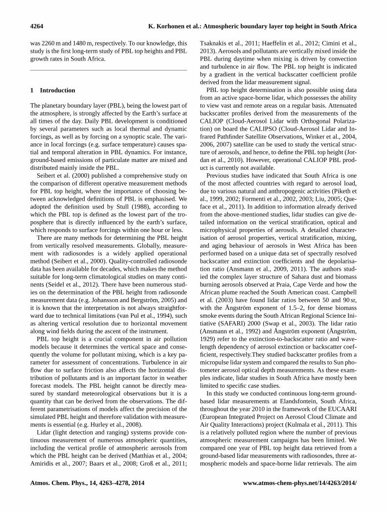
Comparisons of PBL top heights between ground-basedPollyXT lidar and space-borne CALIOP lidar have been per-formed for the 29 common cases. As previously stated, theCALIOP overpasses were between 60 and 110 km from thelidar site. The scatter plot between CALIOP and PollyXT li-dar derived PBL heights shows a good correlation with a cor-relation coefficient of 0.88 (Fig. 9). The majority of our data

Fig. 9. PBL top comparison of 29 common PBL top height obser-vation cases for PollyXT and CALIOP data.

accounts for PBL heights lower than 3 km. The overestima-tion seems to be larger for larger PBL top heights (>1.5 km)(see Fig. 9), rather than being related to the distance betweenthe overpass and the lidar station or the time difference. Inthe cases when CALIOP detected two or more layers, weconsidered the top of the first layer from the ground to be thePBL top height. However, in three cases (out of the total 29),the top of the second layer was taken, since it was obviousfrom the attenuated backscatter profiles of CALIOP that thefirst layer corresponds to a layer inside the PBL. Based onthis comparison data set, the altitude of the first layer of level2 aerosol layer product can be considered being consistentwith the PBL top height determined with ground-based lidarin 90 % of the cases.

4.4 Diurnal PBL cycle

Figure 10 shows the annual average of diurnal PBL evolu-tion for the common data points. The sunrise times variedbetween 05:07 and 06:56, while sunset times ranged between17:23 and 19:05 – these time are indicated with the shadedareas in Fig. 10. The lidar measurements cover both day-time CBL and nocturnal RL heights, similarly to the SAWSmodel.

According to the PollyXT measurements, the daily evolu-tion of the CBL starts approximately 3 to 4 h after sunrise anda daily PBL maximum top height is reached on average 3.5 hafter the solar noon (solar noon at 11:51–12:14 with seasonaldependence). The ECMWF model evaluates the PBL heightonly during convective conditions (daytime) and thereforethe night-time result for PBL height is low. Due to the 3 htemporal resolution, the simulated daily maximum heightsof the PBL top are reached at 14:00 or 17:00 on all daysstudied, which may have a 1.5 h difference between the max-imum PBL top height time measured with the lidar (15:30 on



Fig. 10.PBL diurnal cycle observed in Elandsfontein during 2010. The grey shading indicates the times of sunrise and sunset.

average). From Figure 10, one can identify that the PBL de-velopment starts earlier and is stronger in the ECMWF modelcompared to the PollyXT data (see values between 08:00 and17:00). During the day the best correlations of 0.46 and 0.52were found between the two methods at 14:00 and 17:00, re-spectively. This correlation was only 0.16 at 11:00.

TAPM, with a 1 h temporal resolution follows the CBLevolution well despite systematic underestimation of PBLheight, which was discussed in Sect. 4.3.4. The SAWS modelgives both CBL and RL heights, and the results agree wellfor the latter in comparison to lidar measurement. The BRNmethod used in the SAWS model is sensitive enough to detectinversion layers that occur on the RL top under stable condi-tions, i.e. non-convective atmospheric conditions. The samefeature is also observed in the radiosonde data. The 22:00soundings agree better with the lidar measurement than thesoundings at 10:00.

4.5 Planetary boundary layer characteristics

This section summarises the PBL characteristics determinedwith the PollyXT lidar for 2010 at Elandsfontein. The discus-sion of the SBL is based on the ECMWF and TAPM models.The presented features could be generalised to some extentfor different years (the year 2010 average temperature wasclose to the long-term averages) in southern Africa in areaswith similar surface properties and solar radiation. As shownin Fig. 5, the seasonal cycle of the PBL top height is relativelyexplicit and follows the cycle of solar radiation (Fig. 2b). Onaverage, the PBL top was highest in spring (September andOctober with heights of 2170 and 2260 m with standard de-viations of 790 m and 940 m, respectively), while it was thelowest in winter (May–August with heights of 1450–1790 m)and in January (1210 m), which may be due to low number ofmeasurement days (5). The standard deviations of monthlyaverages were from 17 % (January) up to 42 % (October),

which indicates high variability between the PBL daily topmaxima. The diurnal cycle is also well pronounced (Fig. 10).The evolution of the observed CBL started approximately3 to 4 h after sunrise and the daily PBL top maximum wasreached about 3.5 h after the solar noon. The models fol-lowing the CBL (ECMWF and TAPM) show that the SBLtop during night-time is on average 160 m (monthly averagesvarying from 70 to 270 m). The RL top (defined by the lidar)remains on average at 890 m during the night (monthly av-erages from 450 to 1370 m). The low SBL heights observedsupport earlier findings in South Africa that indicated thatthe night-time domestic pollution originating mainly frominformal and semi-formal settlements is trapped near the sur-face of the earth and heavily impacts local air quality (Ven-ter et al., 2012). The industrial emissions are most probablyreleased and lifted to the RL because of tall stacks. As an ex-ample, all but two power plants owned by the national powercompany have stacks rising up to 200 m or more (Bethlehemand Goldblatt, 1997). Therefore the immediate effect of in-dustrial emissions on air quality is smaller during the night,when the SBL is low.

4.6 PBL growth rates

Figure 11 presents the PBL growth rates determined in2010. All modelled values (Fig. 11b–d) are in relativelygood agreement with the PollyXT measurements presentedin Fig. 10a. The modes of the lidar, the ECMWF model(Fig. 11b) and the SAWS model (Fig. 11c) are 120–180 m h−1 with frequencies of 32.2 %, 34.5 %, and 39.7 %,respectively. The corresponding median values for the lidar,the ECMWF model and the SAWS model are 183, 167 and163 m h−1 with standard deviations of 84, 76 and 74 m h−1,respectively. The median of TAPM (Fig. 11d) at 172 m h−1

(standard deviation 81 m h−1) agrees with the other methodsalthough the standard deviation is the second largest after



Fig. 11.PBL growth rates during the comparison period:(a) PollyXT, (b) ECMWF, (c) SAWS 2 and(d) TAPM.

PollyXT (81 m h−1) and 30.5 % of the values are in the rangeof 120–180 m h−1. The large percentage of values below the120–180 m h−1 range, 32.4 %, can partly explain the previ-ous result of systematical underestimation of the PBL topheight by TAPM. The length of the growth period of theTAPM was typically similar to that of the PollyXT measure-ments with an average of 6.8 h (PollyXT 6.7 h).

5 Comparison to other locations

This study is the first long-term study of PBL top heightsand PBL growth rates in the Southern Hemisphere. The av-erage PBL top height of 1.4± 0.5 km a.g.l. under convectiveconditions (08:00–17:00) is comparably high, with its high-est values and variability in spring (1.6± 0.7 km) and lowervalues in the other seasons (1.3 km). Within Europe, maxi-mum values occurred during summer, e.g. 1.8 km in Leipzig,Germany (Baars et al., 2008) and 1.3 km in Granada, Spain(Granados-Muñoz et al., 2012). In winter both of these stud-ies showed values around 0.8 km. Chen et al. (2001) have re-ported PBL top heights of 1.0 km for a site in Japan in springand autumn, while PBL top heights were 0.4 and 0.7 km inwinter and summer, respectively. Hänel et al. (2012) havereported night-time RL top heights of 0.7 to 1.1 km in thevicinity of Beijing, China, with maximum values in springand summer.

The PBL growth rates found in this study compare wellwith other locations and maximum values coincide with themaximum PBL top heights. PBL growth rates were, thus,highest in spring with 220± 100 m h−1 and lower during theother seasons. On average, growth rates between 100 and 300m h−1 were found. Baars et al. (2008) found growth rates of100 to 300 m h−1 most of the year and 400 to 500 m h−1 in

summer. Chen et al. (2001) reported lower growth rates of 30to 100 m h−1 with peak values of 140 m h−1 in autumn.

6 Summary and conclusions

One year of PBL top height observations done with PollyXT

lidar were compared with three atmospheric models, ra-diosonde measurements and CALIOP space-borne lidar inSouth Africa. It was shown that the lidar is suitable for con-tinuous measurements of daytime PBL and night-time RLwith high temporal data coverage. We had data coverage of49 % for the complete sampling period (60 % if maintenancebreaks are excluded). For the lidar PBL top height determina-tion the WCT method performed well despite frequent com-plex vertical aerosol layer structures caused by large emis-sions from large point sources and biomass burning. The li-dar detected the PBL top height for 86 % of all the measure-ments (42 % of the total time). The best performance in datacoverage and PBL height detection was observed during thedry season (April–September), when rain and cloudy con-ditions had only a minor impact on the measurements andaerosol concentrations were the highest.

The comparison between PollyXT lidar and radiosondemeasurements showed large variation. However, there are afew aspects which are likely to contribute to the discrepan-cies between the two methods. Firstly, the radiosonde launchsite (Pretoria) is 120 km from the lidar site and secondly, wefound cases when entirely stable troposphere resulted in clearfailure in PBL height determination by the BRN method. De-spite their limitations in temporal resolution and PBL topheight determination method, radiosondes have been rou-tinely used for decades and therefore are a valuable methodfor long-term climatology analyses.



The results from the ECMWF model indicated the bestagreement with the lidar data in the annual PBL cycle.Hence, the model predicts the daily PBL top maximumheight well despite its 3 h temporal resolution. In addition,the PBL growth rates agree well with those derived from li-dar data. The performance of the model is the best during thedry season (May–June) with relatively small average over-estimation (8.2 %) of PBL top height when all daytime val-ues (11:00, 14:00 and 17:00) are compared with the PollyXT

data. During spring and summer (October–February) the dif-ferences varied more, which is most probably a combinedresult from weather-related limitations (clouds and precip-itation) of the lidar measurements, as well as maintenancethat was done during two summer months. Both the afore-mentioned reasons lead to a smaller lidar data set during thisrainy season.

The SAWS model performed well in general, notwith-standing the fixed pressure levels with 50 hPa intervals,which results in vertical resolution of about 500 m nearthe surface. The model performed second best with regardto daytime PBL top height evaluation with only slightlylarger mean absolute difference than the lidar measurements(20.6 %). Similar uncertainties were observed as for the ra-diosondes, but the overall performance of the SAWS modelwas relatively good compared to the results from PollyXT andthe ECMWF model. However, the SAWS model underesti-mates the wind speed strongly. About 89 % of the model val-ues were smaller than the measured wind speed. The under-estimation of the wind speed may affect the higher altitudeweather parameters in the model and therefore have conse-quences for the PBL top height determination.

The TAPM has the densest vertical grid of the stud-ied models, but it systematically underestimated the PBLtop height, possibly due to its determination method. Themean relative difference in the comparison between lidar andTAPM is 34.7 %. The modelled values are smaller than PBLtop heights measured with the lidar for 92 % of the cases. Themodel temperature and global radiation compared well withthe measurements, but the model underestimates the windspeed strongly. The mean absolute difference was 23 % andabout 74 % of the model values were smaller than the mea-sured wind speed. The underestimation of the wind speedprobably leads to underestimation of the vertical wind andturbulence, thus underestimation of the PBL top height. Thismay partly explain the observed differences.

The CALIOP level 2 aerosol layer product compares wellwith the PBL top heights from PollyXT lidar. For the totalnumber of 29 cases, the correlation coefficient is 0.88 andfor 90 % of the studied cases, the altitude of the first layer oflevel 2 aerosol layer product can be considered as the PBLtop.

The notable differences found between the methods forPBL top height determination show that one has to be care-ful when using a modelled value for a specific location andtime. Moreover, the use of radiosonde data from a distant site

should be considered carefully. Different approaches couldeven produce different seasonal cycles, as was observed atthe studied site. The elevation of the area and the hilly sur-roundings (surface elevation varies within 200 m) may be re-sponsible for some of the differences depending on the modelgrid (even though it was centred at our site). If the PBL topheights are used in air quality modelling, the possible unre-alistic PBL top height variations will be transferred directlyto the air quality results through the erroneous size of themixing volume for aerosols. More direct measurements ofthe PBL top heights e.g. with lidars can be used to verify themodels. For more detailed model verification studies we rec-ommend the usage of all available model data products andparameters in order to cover all the drivers of PBL dynamics,such as temperature, wind speed, solar radiation, vertical heatflux, surface reflectivity and modelled vegetation parameters.

Acknowledgements.This work has been partly supported by theEuropean Union (in project EUCAARI). The authors acknowledgethe staff of the North-West University for valuable assistance androutine maintenance of the lidar. We also acknowledge Eskom andSasol for their logistical support for measurements at Elandsfontein.

Edited by: L. Ganzeveld

References

Althausen, D., Engelmann, R., Baars, H., Heese, B., Ansmann,A., Müller, D., and Komppula, M.: Portable Raman Lidar Pol-lyXT for Automated Profiling of Aerosol Backscatter, Extinc-tion, and Depolarization, J. Atmos. Ocean. Technol., 26, 2366–2378, 2009.

Amiridis, V., Melas, D., Balis, D. S., Papayannis, A., Founda, D.,Katragkou, E., Giannakaki, E., Mamouri, R. E., Gerasopoulos,E., and Zerefos, C.: Aerosol Lidar observations and model calcu-lations of the Planetary Boundary Layer evolution over Greece,during the March 2006 Total Solar Eclipse, Atmos. Chem. Phys.,7, 6181–6189, doi:10.5194/acp-7-6181-2007, 2007.

Ansmann, A., Riebesell, M., Wandinger, U., Weitkamp, C., Voss,E., Lahmann, W., and Michaelis, W.: Combined Raman elastic-backscatter lidar for vertical profiling of moisture, aerosol extinc-tion, backscatter, and lidar ratio, Appl. Phys. B55, 18–28, 1992.

Ansmann, A., Baars, H., Tesche, M., Müller, D., Althausen, D., En-gelmann, R., Pauliquevis, T., and Artaxo, P.: Dust and smoketrasport from Africa to South America: Lidar profiling overCape Verde and the Amazon rainforest, Geophys. Res. Lett., 36,L11802, doi:10.1029/2009GL037923, 2009.

Ansmann, A., Petzold, A., Kandler, K., Tegen, I., Wendisch, M.,Müllet, D., Weinzierl, B., Müller, T., and Heintzenberg, J.: Sa-haran Mineral Dust Experiments SAMUM-1 and SAMUM-2:what have we learned? Tellus 63B, 403–429, doi:10.1111/j.1600-0889.2011.00555.x, 2011.

Baars, H., Ansmann, A., Engelmann, R., and Althausen, D.: Con-tinuous monitoring of the boundary-layer top with lidar, At-mos. Chem. Phys., 8, 7281–7296, doi:10.5194/acp-8-7281-2008,2008.


http://dx.doi.org/10.5194/acp-7-6181-2007

http://dx.doi.org/10.1029/2009GL037923

http://dx.doi.org/10.1111/j.1600-0889.2011.00555.x

http://dx.doi.org/10.1111/j.1600-0889.2011.00555.x



Bethlehem, L. and Goldblatt, M.: The Bottom Line, Industry and theEnvironment in South Africa. University of Cape Town Press, In-ternational Development Research Centre, ISBN 0-88936-830-9,1997.

Brooks, I. M.: Finding Boundary Layer Top: Application of aWavelet Covariance Transform to Lidar Backscatter Profiles, J.Atmos. Ocean. Technol., 20, 1092–1195, 2003.

Campbell, J. R., Welton, E., Spinhirne, J. D., Ji, Q., Tsay, S. C.,Piketh, S. P., and Barenbrug, M.: Micropulse lidar observationsof tropospheric aerosols over northeastern South Africa duringthe ARREX and SAFARI 2000 dry season experiments, J. Geo-phys. Res., 108, 8497–8530, doi:10.1029/2002JD002563, 2003.

Chen, W., Kuze, H., Uchiyama, A., Suzuki, Y., and Takeuchi, N.:One-year observation of urban mixed layer characteristics atTsukuba, Japan using a micro pulse lidar, Atmos. Environ., 35,4273–4280, doi:10.1016/S1352-2310(01)00181-9, 2001.

Cimini, D., De Angelis, F., Dupont, J.-C., Pal, S., and Haeffelin,M.: Mixing layer height retrievals by multichannel microwaveradiometer observations, Atmos. Meas. Tech., 6, 2941–2951,doi:10.5194/amt-6-2941-2013, 2013.

ECMWF: IFS Documentation – Cy36r1, part 5: Ensemble predic-tion system, ECWMF, 2010a.

ECMWF: IFS Documentation – Cy36r1, part 4: Physical processes,ECMWF, 2010b.

ECMWF: IFS Documentation – Cy36r1, ECMWF, 2010c.Formenti, P., Winkler, H., Fourie, P., Piketh, S., Makgopa, B., Helas,

G., and Andreae, M. O.: Aerosol optical depth over a remotesemi-arid region of South Africa from spectral measurements ofthe daytime solar extinction and the nighttime stellar extinction,Atmos. Res., 62, 11–32, doi:10.1016/S0169-8095(02)00021-2,2002.

Formenti, P., Elbert, W., Maenhaut, W., Haywood, J., Osborne, S.,and Andreae, M. O.: Inorganic and carbonaceous aerosols dur-ing the Southern African Regional Science Initiative (SAFARI2000) experiment: Chemical characteristics, physical properties,and emission data for smoke from African biomass burning, J.Geophys. Res., 108, 8488, doi:10.1029/2002JD002408, 2003.

Granados-Muñoz, M. J., Navas-Guzmán, F., Bravo-Aranda, J.A., Guerrero-Rascado, J. L., Lyamani, H., Fernandez-Galvez,J., and Alados-Arboledas, L.: Automatic determination of theplanetary boundary layer height using lidar: one-year analy-sis over Southeastern Spain., J. Geophys. Res., 117, D18208,doi:10.1029/2012JD017524, 2012.

Groß, S., Gasteiger, J., Freudenthaler, V., Wiegner, M., Geiß,A., Schladitz, A., Toledano, C., Kandler, K., Tesche, M.,Ansmann, A. and Wiedensohler, A.: Characterization of theplanetary boundary layer during SAMUM-2 by means of li-dar measurements. Tellus 63B, 695–705, doi:10.1111/j.1600-0889.2011.00557.x, 2011.

Haeffelin, M., Angelini, F., Morille, Y., Martucci, G., Frey, S.,Gobbi, G. P., Lolli, S., O’Dowd, C. D., Sauvage, L., Xueref-Rémy, I., Wastine, B., Feist, D. G.: Evaluation of Mixing-HeightRetrievals from Automatic Profiling Lidars and Ceilometers inView of Future Integrated Networks in Europe, Bound.-Lay. Me-teorol., 143, 49–75, doi:10.1007/s10546-011-9643-z, 2012.

Hennemuth, B. and Lammert, A.: Determination of the atmosphericboundary layer height from radiosonde and lidar backscatter,Bound.-Lay. Meteorol., 120, 181–200, doi:10.1007/s10546-005-9035-3, 2006.

Hurley, P.: TAPM V4. Part 1: Technical Description. CSIRO Marineand Atmospheric Research Paper No. 25, October 2008. ISBN:978-1-921424-71-7, 2008.

Hurley, P. J., Physick, W. L., and Luhar, A. K.: TAPM: a practi-cal approach to prognostic meteorological and air pollution mod-elling, Environ. Model. Softw., 20, 737–752, 2005a.

Hurley, P., Physick, W., Luhar, A., and Edwards, M.: The Air Pol-lution Model (TAPM) Version 3. Part 2: Summary of some veri-fication studies, CSIRO, Atmos. Res., 72, 20–36, 2005b.

Hurley, P., Edwards, M., and Luhar, A.: TAPM V4. Part 2: Summaryof Some Verification Studies. CSIRO Marine and AtmosphericResearch Paper No. 26, October 2008, ISBN: 978-1-921424-72-4, 2008.

Hänel, A., Baars, H., Althausen, D., Ansmann, A., Engelmann,R., and Sun, J. Y.: One-year aerosol profiling with EU-CAARI Raman lidar at Shangdianzi GAW station: Beijingplume and seasonal variations, J. Geophys. Res., 117, D13201,doi:10.1029/2012JD017577, 2012.

Johansson, C. and Bergström, H.: An auxiliary tool to determine theheight of the boundary layer, Bound.-Lay. Meteorol., 115, 423–432, doi:10.1007/s10546-004-1424-5, 2005.

Jordan, N. S., Hoff, R. M., and Bacmeister, J. T.: Validation ofGoddard Earth Observing System-version 5 MERRA planetaryboundary layer heights using CALIPSO, J. Geophys. Res., 115,D24218, doi:10.1029/2009JD013777, 2010.

Kulmala, M., Asmi, A., Lappalainen, H. K., Baltensperger, U.,Brenguier, J.-L., Facchini, M. C., Hansson, H.-C., Hov, Ø.,O’Dowd, C. D., Pöschl, U., Wiedensohler, A., Boers, R.,Boucher, O., de Leeuw, G., Denier van der Gon, H. A. C., Fe-ichter, J., Krejci, R., Laj, P., Lihavainen, H., Lohmann, U., Mc-Figgans, G., Mentel, T., Pilinis, C., Riipinen, I., Schulz, M.,Stohl, A., Swietlicki, E., Vignati, E., Alves, C., Amann, M.,Ammann, M., Arabas, S., Artaxo, P., Baars, H., Beddows, D.C. S., Bergström, R., Beukes, J. P., Bilde, M., Burkhart, J. F.,Canonaco, F., Clegg, S. L., Coe, H., Crumeyrolle, S., D’Anna,B., Decesari, S., Gilardoni, S., Fischer, M., Fjaeraa, A. M., Foun-toukis, C., George, C., Gomes, L., Halloran, P., Hamburger, T.,Harrison, R. M., Herrmann, H., Hoffmann, T., Hoose, C., Hu,M., Hyvärinen, A., Hõrrak, U., Iinuma, Y., Iversen, T., Josipovic,M., Kanakidou, M., Kiendler-Scharr, A., Kirkevåg, A., Kiss, G.,Klimont, Z., Kolmonen, P., Komppula, M., Kristjánsson, J.-E.,Laakso, L., Laaksonen, A., Labonnote, L., Lanz, V. A., Lehtinen,K. E. J., Rizzo, L. V., Makkonen, R., Manninen, H. E., McMeek-ing, G., Merikanto, J., Minikin, A., Mirme, S., Morgan, W. T.,Nemitz, E., O’Donnell, D., Panwar, T. S., Pawlowska, H., Pet-zold, A., Pienaar, J. J., Pio, C., Plass-Duelmer, C., Prévôt, A.S. H., Pryor, S., Reddington, C. L., Roberts, G., Rosenfeld, D.,Schwarz, J., Seland, ø., Sellegri, K., Shen, X. J., Shiraiwa, M.,Siebert, H., Sierau, B., Simpson, D., Sun, J. Y., Topping, D.,Tunved, P., Vaattovaara, P., Vakkari, V., Veefkind, J. P., Viss-chedijk, A., Vuollekoski, H., Vuolo, R., Wehner, B., Wildt, J.,Woodward, S., Worsnop, D. R., van Zadelhoff, G.-J., Zardini,A. A., Zhang, K., van Zyl, P. G., Kerminen, V.-M., S Carslaw,K., and Pandis, S. N.: General overview: European Integratedproject on Aerosol Cloud Climate and Air Quality interactions(EUCAARI) – integrating aerosol research from nano to globalscales, Atmos. Chem. Phys., 11, 13061–13143, doi:10.5194/acp-11-13061-2011, 2011.


http://dx.doi.org/10.1029/2002JD002563

http://dx.doi.org/10.1016/S1352-2310(01)00181-9

http://dx.doi.org/10.5194/amt-6-2941-2013

http://dx.doi.org/10.1016/S0169-8095(02)00021-2

http://dx.doi.org/10.1029/2002JD002408

http://dx.doi.org/10.1029/2012JD017524

http://dx.doi.org/10.1111/j.1600-0889.2011.00557.x

http://dx.doi.org/10.1111/j.1600-0889.2011.00557.x

http://dx.doi.org/10.1007/s10546-011-9643-z

http://dx.doi.org/10.1007/s10546-005-9035-3

http://dx.doi.org/10.1007/s10546-005-9035-3

http://dx.doi.org/10.1029/2012JD017577

http://dx.doi.org/10.1007/s10546-004-1424-5

http://dx.doi.org/10.1029/2009JD013777




Laakso, L., Vakkari, V., Virkkula, A., Laakso, H., Backman, J., Kul-mala, M., Beukes, J. P., van Zyl, P. G., Tiitta, P., Josipovic, M.,Pienaar, J. J., Chiloane, K., Gilardoni, S., Vignati, E., Wieden-sohler, A., Tuch, T., Birmili, W., Piketh, S., Collett, K., Fourie, G.D., Komppula, M., Lihavainen, H., de Leeuw, G., and Kerminen,V.-M.: South African EUCAARI measurements: seasonal varia-tion of trace gases and aerosol optical properties, Atmos. Chem.Phys., 12, 1847–1864, doi:10.5194/acp-12-1847-2012, 2012.

Lai, L. and Cheng, W. L.: Air quality influenced by urban heat is-land coupled with synoptic weather patterns, Sci. Total Environ.,4, 2724–2733, 2009.

Landman, S., Engelbrecht, F. A., Engelbrecht, C. J., Dyson, L. L.,and Landman, W.: A short-range prediction system based on amulti-model approach, Water SA, 38, ISSN 0378-4738, 2012.

Liu, L.: Improving GCM Aerosol Climatology using satellite andground based measurements, paper presented at 15th ARM Sci-ence Team Meeting, Atmos. Radiat. Meas. (ARM) Program,Daytona Beach, Florida, 14–18 March, 2005.

Lourens, A. S. M., Beukes, J. P., van Zyl, P. G., Fourie, G. D.,Burger, J. W., Pienaar, J. J., Read, C. E. and Jordaan, J. H. L.,Spatial and Temporal assessment of Gaseous Pollutants in theMpumalanga Highveld of South Africa, South Afr. J. Sci., 107,8 pp. doi:10.4102/sajs.v107i1/2.269, 2011.

Lourens, S. M., Butler, T. M., Beukes, J. P., van Zyl, P. G.,Beirle, S., Wagner, T., Heue, K.-P., Pienaar, J. J., Fourie, G.D., and Lawrence, M. G.: Re-evaluating the NO2 hotspot overthe South African Highveld, South Afr. J. Sci., 108, 6 pp..doi:10.4102/sajs.v108i11/12.1146, 2012.

Luhar, A. K. and Hurley P. J.: Application of a prognostic modelTAPM to sea-breeze flows, surface concentrations, and fumigat-ing plumes, Environ. Model. Softw., 19, 591–601, 2004.

Matthias, V., Balis, D., Bösenberg, J., Eixmann, R., Iarlori, M.,Komguem, L., Mattis, I., Papayannis, A., Pappalardo, G., Per-rone, M. R., and Wang, X.: Vertical aerosol distribution over Eu-ropr: Statistical analysis of Raman lidar data from 10 EuropeanAerosol Research Lidar Network (EARLINET) stations, J. Geo-phys. Res., 109, D18201, doi:10.1029/2004JD004638, 2004.

Menut, L., Flamant, C., Pelon, J., and Flamant, P. H.: Urbanboundary-layer height determination from lidar measurementsover the Paris area, Appl. Opt., 38, 6, 945–954, 1999.

Piketh, S. J., Annegarn, H. J., and Tyson, P. D.: Lower troposphericaerosol loadings over South Africa: The relative contribution ofaeolian dust, industrial emissions, and biomass burning, J. Geo-phys. Res., 104, 1597–1607, doi:10.1029/1998JD100014, 1999.

Piketh, S. J., Swap, R. J., Maenhaut, W., Annegarn, H. J., andFormenti, P.: Chemical evidence of long-range atmospherictransport over southern Africa, J. Geophys. Res., 107, 4817,doi:10.1029/2002JD002056, 2002.

Queface, A. J., Piketh, S. J., Eck, T. F., Tsay, S. C., and Mavume, A.F.: Climatology of aerosol optcal properties in Southern Africa,Atmos. Environ., 45, 2910–2921, 2011.

Raghunandan, A., Scott, G., Zunckel, M., and Carter, W.: TAPMverification in South Africa: modelling surface meteorology atAlexander Bay and Richards Bay, Report done on behalf CSIRNatural Resources and the Environment, Congella, 2008.

Seibert, P., Beyrich, F., Gryning, S.-E., Joffre, S., Rasmussen, A.,and Tecier, P.: Review and intercomparison of operational meth-ods for the determination of the mixing height, Atmos. Environ.,34, 1001–1027, 2000.

Seidel, D. J., Zhang, Y., Beljaars, A., Golaz, J.-C., Jacobson, A. R.,and Medeiros, B.: Climatology of the planetary boundary layerover the continental United States and Europe, J. Geophys. Res.,117, D17106, doi:10.1029/2012JD018143, 2012.

Stull, R. B.: An introduction to boundary layer meteorology, KluwerAcademic Publishers, ISBN: 90-277-2768-6, 1988.

Stull, R. B.: Meteorology for Scientists and Engineers, Second Edi-tion, Brooks&Cole, ISBN: 0-534-37214-7, 2000.

Swap, R. J., Annegarn, H. J., Suttles, J. T., King, M. D., Plat-nick, S., Privette, J. L., and Scholes, R. J.: Africa burning:A thematic analysis of the Southern African Regional Sci-ence Initiative (SAFARI 2000), J. Geophys. Res., 108, 8465,doi:10.1029/2003JD003747, 2003.

Troen, I. B. and Mahrt, L.: A simple model of the AtmosphericBoundary Layer; sensitivity to surface evaporation. Bound.-Lay.Meteorol., 37, 129–148, 1986.

Tsaknakis, G., Papayannis, A., Kokkalis, P., Amiridis, V., Kam-bezidis, H. D., Mamouri, R. E., Georgoussis, G., and Avdikos,G.: Inter-comparison of lidar and ceilometer retrievals for aerosoland Planetary Boundary Layer profiling over Athens, Greece. At-mos. Meas. Tech., 4, 1261–1273, doi:10.5194/amt-4-1261-2011,2011.

van Pul, W. A. J., Holtslag, A. A. M., and Swart, D. P. J.: A com-parison of atmospheric boundary layer heights inferred routinelyfrom lidar and radiosondes at noon, Bound.-Layer Meteorol., 68,173–191, 1994.

Vaughan, M. A., Winker, D. M., and Powell, K. A.: CALIOP Algo-rithm Theoretical Basis Document Part 2: Feature Detection andLayer Properties Algorithms, available at:http://www-calipso.larc.nasa.gov/resources/pdfs/PC-SCI-202_Part2_rev1x01.pdf(last access: 28 June 2013), 2005.

Venter, A. D., Vakkari, V., Beukes, J. P., van Zyl, P. G., Laakso,H., Mabaso, D., Tiitta, P., Josipovic, M., Kulmala, M., Pienaar, J.J., and Laakso, L.: An air quality assessment in the industrialisedwestern Bushveld Igneous Complex, South Africa, S. Afr. J. Sci.,108, 84–93, doi:10.4102/sajs.v108i9/10.1059, 2012.

Winker, D., Hostetler, C., and Hunt, W.: CALIOP: The CALIPSOLidar, Proc. 22nd International Laser Radar Conference (ESASP561), Matera, Italy, 941–944, Vol. 6409 (SPIE, Bellingham, WA2006), 640902, 2004.

Winker, D., Vaughan, M., and Hunt, W., The CALIPSO mis-sion and initial results from CALIOP, Proc. SPIE, 6409,doi:10.1117/12.698003, 2006.

Winker, D. M., Hunt, W. H., and McGill, M. J.: Initial perfor-mance assessment of CALIOP, Geophys. Res. Lett., 34, L19803,doi:10.1029/2007GL030135, 2007.

Zawar-Reza, P. and Sturman, A.: Application of airshed modellingto the implementation of the New Zealand National Environmen-tal Standards for air quality, Atmos. Environ., 42, 8785–8794,2008.

Ångström, A.: On the atmospheric transmission of Sun radiationand on dust in the air, Geograf. Ann., 11, 156–166, 1929.



http://dx.doi.org/10.4102/sajs.v107i1/2.269


http://dx.doi.org/10.1029/2004JD004638

http://dx.doi.org/10.1029/1998JD100014

http://dx.doi.org/10.1029/2002JD002056

http://dx.doi.org/10.1029/2012JD018143

http://dx.doi.org/10.1029/2003JD003747

http://dx.doi.org/10.5194/amt-4-1261-2011




http://dx.doi.org/10.1117/12.698003

http://dx.doi.org/10.1029/2007GL030135

atmospheric boundary layer top height in south africa ... · atmospheric boundary layer top height...

Documents