atmosphere - ocean dynamics
TRANSCRIPT
Exercises in
atmosphere - ocean dynamics
by
Tore Furevik
Geophysical Institute
University of Bergen, NorwayBergen, December 2005

CONTENTS i
Contents
1 The equation of state 1
2 Hydrostatic balance and static stability 3
3 Local and total time derivatives 6
4 Diffusion 7
5 Coriolis force 9
6 Inertial Oscillations 11
7 Short and long waves 13
8 Dispersion 15
9 Shallow water waves 17
10 Tides in channels and bays 19
11 Internal waves 22
12 A floating bridge 25
13 Internal waves in a continuously stratified fluid 27
14 Lee waves 29
15 Normal modes 31
16 Geostrophic adjustment in a two-layer fluid 35
17 Long waves in a fluid that is rotating 38
18 Tsunami 40
19 Thermal wind I: The Denmark Strait overflow 42
20 Thermal wind II: The Norwegian Coastal Current 44
21 Available potential energy 47
22 Vorticity dynamics 49
23 Ekman spiral 51
24 Ekman transports and Ekman pumping 53
25 Storm surge 55
26 Coastal upwelling with weak winds 56
27 Coastal upwelling with strong winds 57
28 Topographic waves 59
CONTENTS ii
29 Equatorial Kelvin Waves 61
30 Planetary waves 64

1
1 The equation of state
The equation of state is fundamental in both atmospheric and ocean dynamics. Usually itrelates the density to the pressure, temperature and the chemical composition in the fluid. Wewill here look at some of the properties for the atmosphere and ocean. The motivation forthis exercise is to get used to functions of more than one variable, and to assess some of thefundamental properties of air and sea water density.
A. Air density
Use Figure 1(a) to answer the following questions:
1a) How is air density changing with increasing temperature (T ) or humidity (q)? Mathe-matically, that is ∂ρ
∂T and ∂ρ∂q .
1b) Can you by looking at the figure explain why the air is rising in the low latitudes (nearEquator), and sinking at the poles?
1c) What is (approximately) the virtual temperature of saturated air at 25C?
1d) What do you think happens if saturated air at 5C comes in contact with (mixes with)saturated air at 15C?
B. Ocean density
Use Figure 1(b) to answer the following questions:
1e) How is ocean density changing with increasing salinity, temperature or pressure ( ∂ρ∂S , ∂ρ
∂T ,
or ∂ρ∂p)?
1f) How is ∂ρ∂T changing with salinity, temperature or pressure ( ∂2ρ
∂T∂S , ∂2ρ∂T 2 , or ∂2ρ
∂T∂p)?
1g) For what temperatures are the density change with pressure, the compressibility, largest(this effect is know as the thermobaric effect)?
1h) In the figure we have marked two water masses with crosses. They represent typicalTS values for water masses in the Greenland Sea (cold, fresh) and in the Mediterranean(warm, salty). Which of the two is heaviest at surface pressure? Which is heaviest at3000m depth? Do you think this has any implications for the temperatures in the deepocean?
1i) What do you think may happen if two water masses having the same density, but differenttemperatures and salinities, mix (this effect is know as caballing)?
1j) In the Antarctica melting and freezing processes exist down to almost 2000m depthsbeneath the floating ice shelves. What can you say about the temperatures of the watermasses formed under these extreme conditions?
1k) The deepest water masses in the World Oceans are formed in the Antarctica (WeddellSea). Can you suggest why this is so?

2
(a)
−40 −30 −20 −10 0 10 20 30 400
0.005
0.01
0.015
0.02
0.025
0.03
0.035
0.04
Temperature (°C)
Spec
ific h
umid
ity (k
g/kg
)
Air density (kg m−3) at 1000 mb
1.1
1.15
1.2
1.25
1.3
1.35
1.4
1.45
(b)
33 34 35 36 37 38 39
−4
−2
0
2
4
6
8
10
12
14
16
18
Salinity (psu)
Tem
pera
ture
(° C)
Ocean density (kg m−3) at surface and 3000 db (~3000m)
1025
1026
10271028
1029
1030
1031
1037
1038
1039
1040
1041
1041
1042
1043
1044
1045
Figure 1: (a) Air density (thin curves) as functions of temperature and specific humidity at1000 mb (near sea level). Thick line shows the humidity at saturation. (b) Ocean density(thin curves) as functions of salinity and temperature at surface pressure (solid lines) andat approximately 3000m depths (dashed lines). The two solid lines show the freezing pointtemperatures at the two depths. The two stars represent water masses in the Greenland Sea(cold, fresh) and in the Mediterranean (warm, salty).
3
2 Hydrostatic balance and static stability
By the standard definition of a (x, y, z) coordinate system, the acceleration of gravity (g) isalways pointing in the negative z direction. For an atmosphere or an ocean at rest, or wherevertical accelerations are small, there will be a balance between the gravity and the pressureforces on the fluid. In this exercise we will learn more about the hydrostatic balance and theconcept of static stability.
A. Hydrostatic balance
We start by making a sketch of the pressure forces acting on a small volume element withlength, width and height given by δx, δy, and δz (see Fig. 3.1 in Gill).
2a) Show that the net pressure force in the z direction will be given by −δxδyδz ∂p∂z , and that
the net pressure force per unit mass is − 1ρ∇p, where ∇ ≡ ( ∂
∂x , ∂∂y , ∂
∂z ).
2b) Explain that if the fluid parcel (volume element) is going to be at rest, there has to be abalance between pressure forces and gravity given by ∂p
∂z = −ρg, or written as gradientsof pressure and geopotential as ∇p + ρ∇Φ = 0.
2c) What is the air pressure 1000m above ground, if mean air density is 1.2 kgm−3 and theair pressure at the ground is 1000 mb (= 105Nm−2)?
2d) What is the water pressure at 1000 m depth if mean ocean density is 1030 kgm−3 and thewater pressure at the surface is 1000 mb?
B. Static Stability
Often it is of great interest to get a measure for the stability of the air column or of the oceancolumn. If for instance the air column is heated from below (during a sunny day), the air nearthe ground will loose density, and may start to rise and mix with the air above. Similarly, ifthe water column is cooled from the top (winter cooling), the water near the surface will gaindensity, and may start to sink. The process of mixing air or water by vertical motion, is knownas convection.
2e) Can you think of other meteorological or oceanographic processes that may contribute tochange the stability of the air or water column?
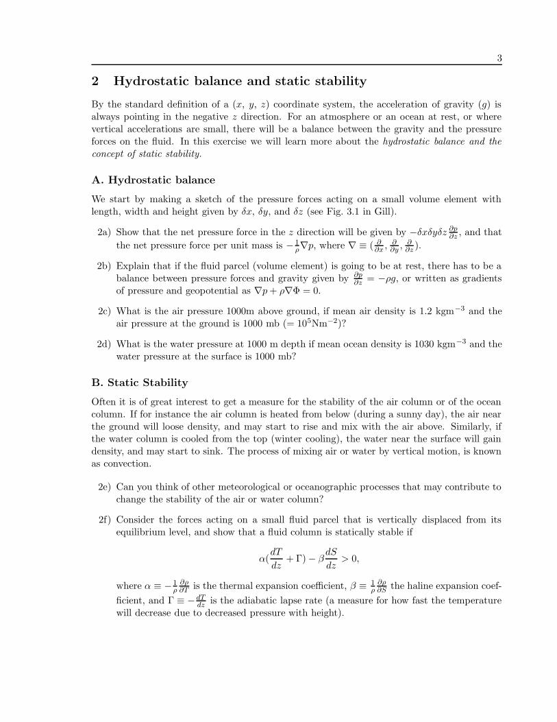
2f) Consider the forces acting on a small fluid parcel that is vertically displaced from itsequilibrium level, and show that a fluid column is statically stable if
α(dT
dz+ Γ) − β
dS
dz> 0,
where α ≡ − 1ρ
∂ρ∂T is the thermal expansion coefficient, β ≡ 1
ρ∂ρ∂S the haline expansion coef-
ficient, and Γ ≡ − dTdz is the adiabatic lapse rate (a measure for how fast the temperature
will decrease due to decreased pressure with height).

4
2g) Show that if a fluid element in a statically stable water column is displaced vertically, itwill start to oscillate with a frequency N given by
N2 = gα(dT
dz+ Γ) − gβ
dS
dz.
What do we call this frequency?
2h) In Figure 2 we have shown measurements of (potential) temperature, salinity, and (po-tential) density from a station between Greenland and Spitsbergen. Use the approximateexpression for the frequency above,
N2 = −g
ρ
dρ
dz,
where ρ is the potential density, to calculate the frequency (N) over the intervals 0-50 m,50-80m, and 2000-2500m (suggestion: instead of using dρ/dz in the equation above, usefinite differences, for instance δρ ≈ 0.1 kgm−3 and δz = 50 m for the first case).
2i) What are the three corresponding period of oscillations?
2j) What can you say about the stability in the three cases?

5
(a)
4 5 6
0
10
20
30
40
50
60
70
80
90
100
Dept
h (m
)
Pot. temperature (°C)34.8 35 35.2
0
10
20
30
40
50
60
70
80
90
100
Salinity (psu)
CTD profile in the Fram Strait
27.5 27.6 27.7 27.8
0
10
20
30
40
50
60
70
80
90
100
σt (kg m−3)
(b)
−2 0 2 4 6
0
500
1000
1500
2000
2500
3000
Dept
h (m
)
Pot. temperature (°C)34.8 35 35.2
0
500
1000
1500
2000
2500
3000
Salinity (psu)
CTD profile in the Fram Strait
27.6 27.8 28 28.2
0
500
1000
1500
2000
2500
3000
σt (kg m−3)
Figure 2: Measured profile of potential temperature, salinity and potential density (in terms ofσt units, i.e. ρ− 1000 kgm−3) at a station in the Fram Strait. (a) shows the upper 100 meters,and (b) shows the entire water column.

6
3 Local and total time derivatives
When a fluid is in motion, its properties (speed, temperature, chemical compositions, etc) willbe a function of both spatial position (x ≡ xi + yj + zk) and time (t). Here we will illuminatethe differences and properties of the local and total time derivatives1.
3a) Show that the total derivative of a property γ is given by
Dγ
Dt≡ ∂γ
∂t+ u · ∇γ.
3b) At a station the temperature is measured to be 15C, and it is falling at a constant rate of2C per hour. The wind is 15ms−1 straight from the north. At the same time a station 100km to the north measures 5C. The temperature is falling with the same rate everywhere.Estimate the rate of temperature change (C per hour) of the air particles as they movetowards south.
3c) Another day the station above measure the wind speed to be 10ms−1 straight from thenorth, and it is increasing at a rate of 5ms−1 per hour. At the same time the station100km to the north measures a wind speed of only 6ms−1, again straight from the north.The increase in wind speed is the same everywhere. What is the mean accelleration ofthe particles as they move towards the south?
3d) During a 1-hour period, two boats pass close to a fishing boat who is laying still. Thespeed of the boats and the recorded pressure changes at the three boats during the passage(1 hour interval) are:
Boat Speed Pressure change
1 5m/s straight north no change2 10 m/s straight east -2 mb3 no speed +1 mb
What is the magnitude and the direction of the maximum change in pressure (suggestion:calculate the pressure gradient ∇p and use Pythagoras)?
1This exercise is partly from Wallace and Hobbs.
7
4 Diffusion
Despite the fact that this course is mainly about dynamics, atmospheric and ocean dynamicsare closely connected to the distribution of the density field. Horizontal density contrasts willset up horizontal pressure forces which again will lead to accelerations and motion. At thesame time diffusion and mixing between the different water masses will always act to reducedensity gradients and thus the pressure forces. Here we will have a brief look at the diffusionequations2.
4a) Consider the balance of salt (or specific humidity) for a small volume element fixed inspace. If the density is ρ, the salinity (or specific humidity) is S, and the diffusivity ofsalt in sea water (or water vapour in the atmosphere) is κD, show that the mass balancefor the salinity in the fixed volume becomes
∂ρS
∂t+ ∇ · (ρSu− ρκD∇S) = 0.
4b) Show that when variations in density and in the diffusivity can be neglected, the equationcan be written
DS
Dt= κD∇2S.
Typical values for the diffusivity is 1.5×10⁻⁹m2s−1 for salt in water and 2.4×10⁻⁵m2s−1
for water vapour in the atmosphere.
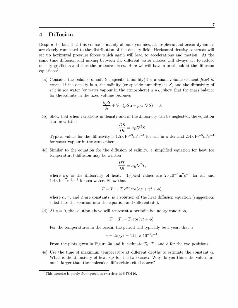
4c) Similar to the equation for the diffusion of salinity, a simplified equation for heat (ortemperature) diffusion may be written
DT
Dt= κH∇2T,
where κH is the diffusivity of heat. Typical values are 2×10⁻⁵m2s−1 for air and1.4×10−7m2s−1 for sea water. Show that
T = T0 + T1eαz cos(αz + γt + φ),
where α, γ, and φ are constants, is a solution of the heat diffusion equation (suggestion:substitute the solution into the equation and differentiate).
4d) At z = 0, the solution above will represent a periodic boundary condition,
T = T0 + T1 cos(γt + φ).
For the temperatures in the ocean, the period will typically be a year, that is
γ = 2π/yr = 1.99 × 10⁻⁷s−1.
From the plots given in Figure 3a and b, estimate T0, T1, and φ for the two positions.
4e) Use the time of maximum temperature at different depths to estimate the constant α.What is the diffusivity of heat κH for the two cases? Why do you think the values aremuch larger than the molecular diffusivities cited above?
2This exercise is partly from previous exercises in GFO110.

8
(a)
Jan Feb Mar Apr May Jun Jul Aug Sep Oct Nov Dec Jan
0
50
100
150
200
250
300
Month of year
Dept
h (m
)
Annual cycle in temperature at 50°N, 30°W
10 10
10
10
11
11
11 11
11
12
12
12
13
13
14 14
15
(b)
Jan Feb Mar Apr May Jun Jul Aug Sep Oct Nov Dec Jan
0
50
100
150
200
250
300
Month of year
Dept
h (m
)
Annual cycle in temperature at 70°N, 0°W
3
4
4
4
4
4
4
4
5
5
5
5
6
6
7
7
8
9
Figure 3: Annual cycle in temperatures at a position in (a) The North Atlantic, and (b) TheNorwegian Sea.
9
5 Coriolis force
In this exercise we investigate the relations between acceleration in a rotating coordinate systemand acceleration in a fixed system. In particular, we will look at the two terms known as thecentrifugal and Coriolis accelerations.
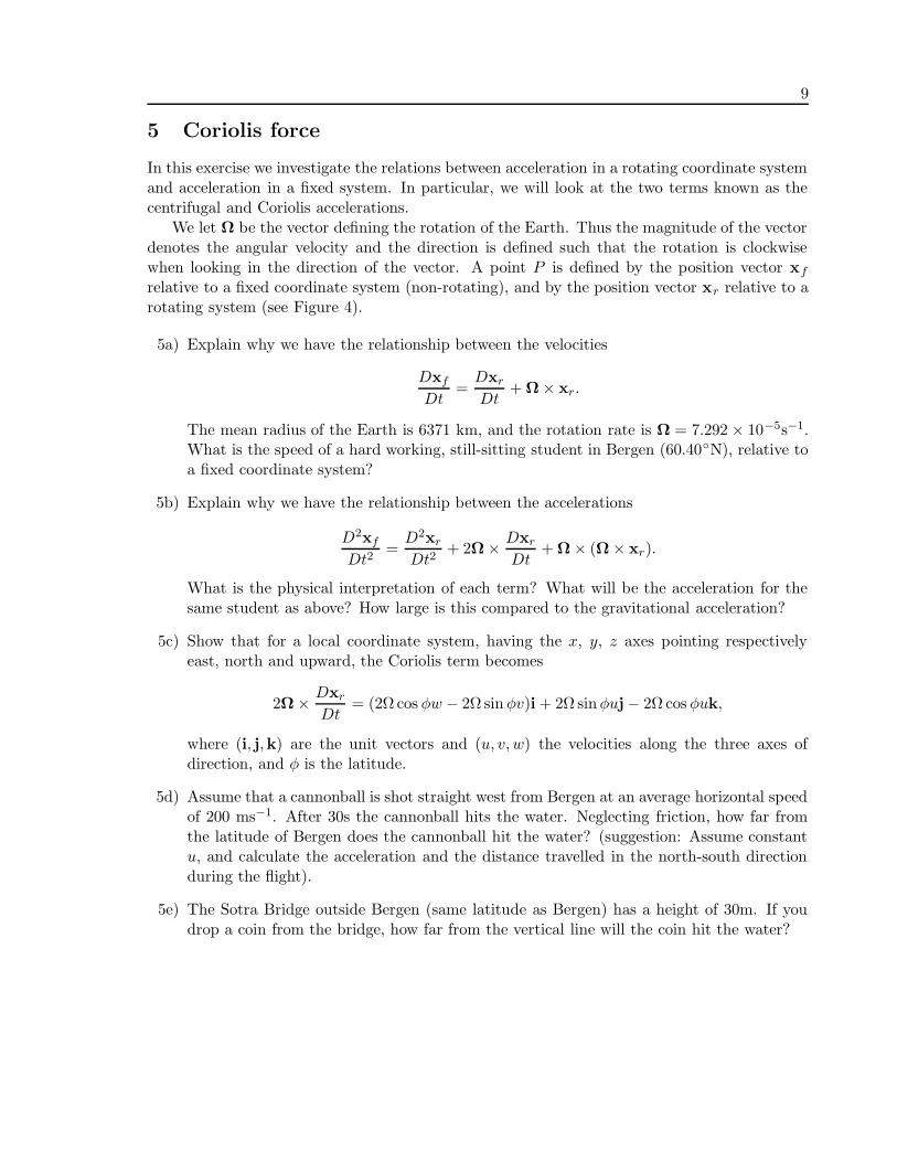
We let Ω be the vector defining the rotation of the Earth. Thus the magnitude of the vectordenotes the angular velocity and the direction is defined such that the rotation is clockwisewhen looking in the direction of the vector. A point P is defined by the position vector xf
relative to a fixed coordinate system (non-rotating), and by the position vector xr relative to arotating system (see Figure 4).
5a) Explain why we have the relationship between the velocities
Dxf
Dt=
Dxr
Dt+ Ω× xr.
The mean radius of the Earth is 6371 km, and the rotation rate is Ω = 7.292 × 10⁻⁵s−1.What is the speed of a hard working, still-sitting student in Bergen (60.40N), relative toa fixed coordinate system?
5b) Explain why we have the relationship between the accelerations
D2xf
Dt2=
D2xr
Dt2+ 2Ω× Dxr
Dt+ Ω× (Ω× xr).
What is the physical interpretation of each term? What will be the acceleration for thesame student as above? How large is this compared to the gravitational acceleration?
5c) Show that for a local coordinate system, having the x, y, z axes pointing respectivelyeast, north and upward, the Coriolis term becomes
2Ω× Dxr
Dt= (2Ω cos φw − 2Ω sin φv)i + 2Ω sinφuj− 2Ω cos φuk,
where (i, j,k) are the unit vectors and (u, v, w) the velocities along the three axes ofdirection, and φ is the latitude.
5d) Assume that a cannonball is shot straight west from Bergen at an average horizontal speedof 200 ms−1. After 30s the cannonball hits the water. Neglecting friction, how far fromthe latitude of Bergen does the cannonball hit the water? (suggestion: Assume constantu, and calculate the acceleration and the distance travelled in the north-south directionduring the flight).
5e) The Sotra Bridge outside Bergen (same latitude as Bergen) has a height of 30m. If youdrop a coin from the bridge, how far from the vertical line will the coin hit the water?
10
P
xr
r
Ω
Ω × xr
Figure 4: A point P with fixed position xr in a frame of reference rotating with angular velocityΩ about an axis through O, will move in the circular path shown. Velocity will be 2Ω×xr andacceleration −∇( 1
2Ω2r2) (redrawn from Gill, fig. 4.5).

11
6 Inertial Oscillations
In some of the previous exercises we looked on the effects of a rotating Earth on the motionsof a particle relative to the Earth. When looking at relatively small time scales with originalvelocity being along axis 1 (x direction), we only have to consider the effect the velocity inthis direction has on the acceleration and velocity in the directions normal to it, for instancealong axis 2 (y direction). If, however, time scales are large, the velocity along axis 2 will givea feedback to the velocity along axis 1. This give rise to circular motion, known as inertialoscillations.
6a) The equation of motion is
Du
Dt+ 2Ω × u = −1
ρ∇p − g + ν∇2u.
Explain what the different terms in the equation represent.
6b) Show that if no external forces are acting on a particle, and we assume no vertical motion,the equation of motion simplifies to
∂u
∂t− fv = 0, and
∂v
∂t+ fu = 0,
where f = 2Ω sinφ is the Coriolis parameter (φ is latitude).
6c) Show that the equation of motion for each of the components may be written
∂2u
∂t2+ f2u = 0, and
∂2v
∂t2+ f2v = 0.
6d) Show by inserting into the equations above that the solutions become
u = U sin(ft + δ), and v = U cos(ft + δ),
where U and δ are constants.
6e) Integrate the two solutions for u and v to get the variations in x and y positions as functionof time (this we call trajectories). Show that the trajectories become circles, given by theequation
(x − x0)2 + (y − y0)
2 = (U
f)2.
Such motion is known as inertial oscillation.
6f) At the latitude of Bergen (60.40N), what is the period of such rotations? And what isthe radius of the circles if the flow speed is 0.1 ms−1? What is the radius at the NorthPole or at the Equator?
6g) In Figure 5 we show some famous current meter measurements taken in the Baltic Sea (at57.8N) in 1936. What is the theoretical period of the inertial oscillations at this location?What is the typical speed of the current? Why do you think the radius of the inertialoscillations decreases with time?

12
Figure 5: Current measurements in the Baltic in 1936. The plot show trajectories (progressivevector diagram) based on current meter measurements in a fixed point. The time intervalbetween each tick is 12 hours (Gill, fig. 8.3).

13
7 Short and long waves
We will in this exercise look at the properties of non-rotating surface gravity waves. As allsurface perturbations (deviations from equilibrium) can be viewed as a superposition of aninfinite number of trigonometric functions (Fourier components), many general properties ofwaves can be derived from looking at an individual component.
For simplicity, we put the x axis along the direction of the wave propagation, and assumeconstant air pressure (p0), sea water density (ρ0), and depth (H). A sketch of the system isgiven in Figure 6.
7a) The equations that determine this problem, are the equation of motion for the x and zdirections, and the continuity equation,
∂u
∂t= − 1
ρ0
∂p
∂x,
∂w
∂t= − 1
ρ0
∂p
∂z− g,
∂u
∂x+
∂w
∂z= 0.
Explain what assumptions that have been made to simplify the general equations ofmotion to the three equations above.
7b) Write the pressure in the fluid p as a sum of the equilibrium pressure p0(z) and theperturbation pressure p′(x, z, t), and derive the Laplace equation for the perturbationpressure
∂2p′
∂x2+
∂2p′
∂z2= 0.
7c) Give the physical explanation for the kinematic and dynamic boundary conditions for thissystem, that is w(0) = ∂η/∂t, w(−H) = 0, and p′(0) = ρ0gη.
7d) We write the surface elevation on the form η = η0 cos(kx − ωt), where η0 is amplitude,k = 2π/λ the wavenumber (λ is the wave length), and ω is the frequency. We furtherassume that the pressure perturbation is proportional to η, that is
p′ = F (z)η0 cos(kx − ωt).
Show that Laplace equation gives
F (z) = C cosh[k(z + δ)],
where C and δ are integration constants to be determined by the boundary condition.
7e) Use the dynamic boundary condition to determine the constant C.
7f) Find the solution for the vertical velocity w, and use the kinematic boundary conditionat the bottom to show that the total solution for the perturbation pressure becomes
p′ =ρ0gη0 cosh[k(z + H)] cos(kx − ωt)
cosh(kH).

14
z=0
z=−H
ρ0
p0 x
η=η(x,t)
Figure 6: Sketch of a surface gravity wave.
7g) Use the last boundary condition to derive the dispersion relation
ω2 = gk tanh(kH).
What is the velocity of the wave?
7h) We shall now look at two extreme cases, one where wave lengths are long compared tobottom depth, kH 1, and one where wave lengths are short compared to bottom depth,kH 1. What are the frequencies and phase speeds of the two types of waves?
7i) What are the two velocity components u, and w for the short waves (kH 1)?
7j) Integrate the two velocity components with respect to time, and show that the paths ofthe fluid particles become circles with radius decreasing exponentially with depth. Atwhat depth is the radius reduced to exp(−1) of the surface value (reduced to 37%)? Howdeep will a 10 m long wave reach? What about a 100 m long wave?
7k) Sitting at the coast west of Bergen, you notice that waves coming in from a storm center inthe North Atlantic are typically 100 m long. 12 hours later, wave lengths have decreasedto 50 m. Assuming that the waves are short compared to the depth, what is the distanceto the storm center?
15
8 Dispersion
In the previous exercise we looked at a single wave. We will now extend the analysis to twowaves, define the group velocity, and investigate more properties of short and long waves.
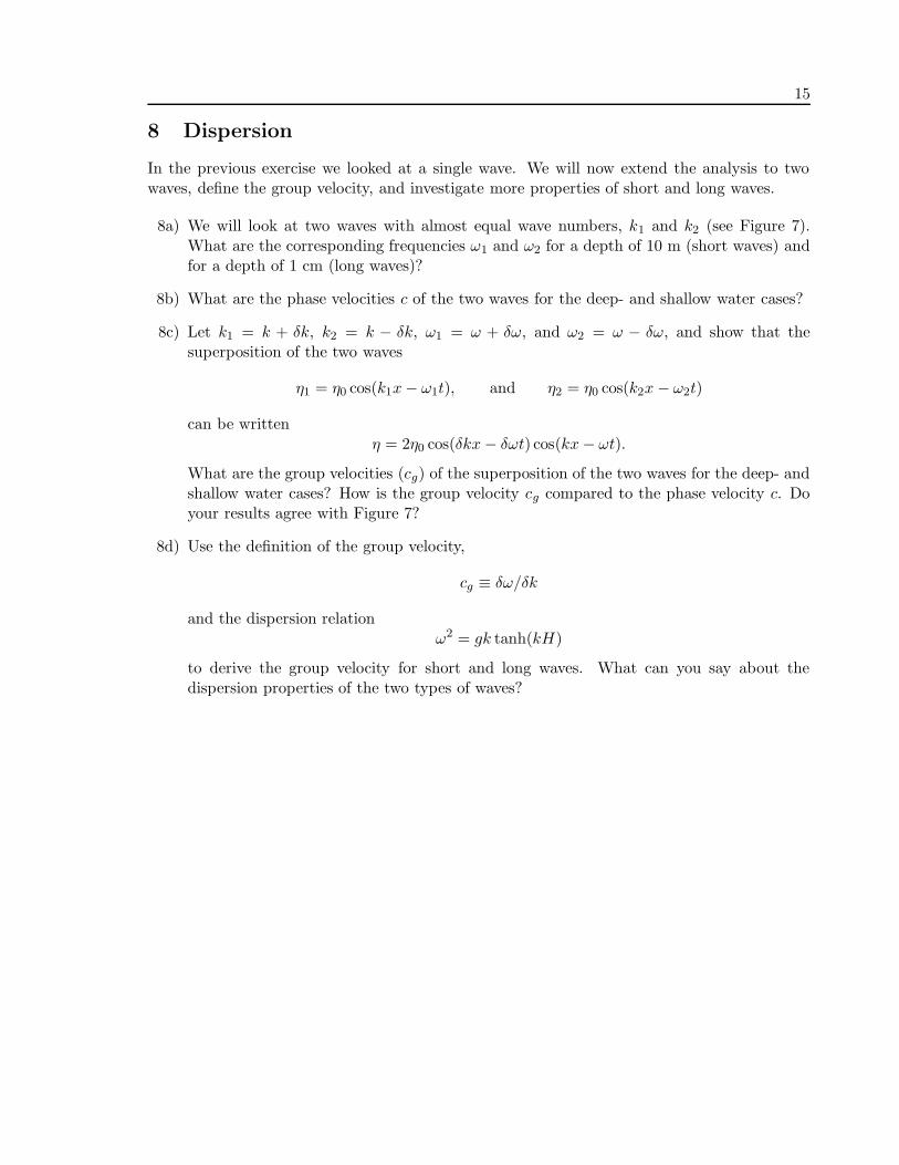
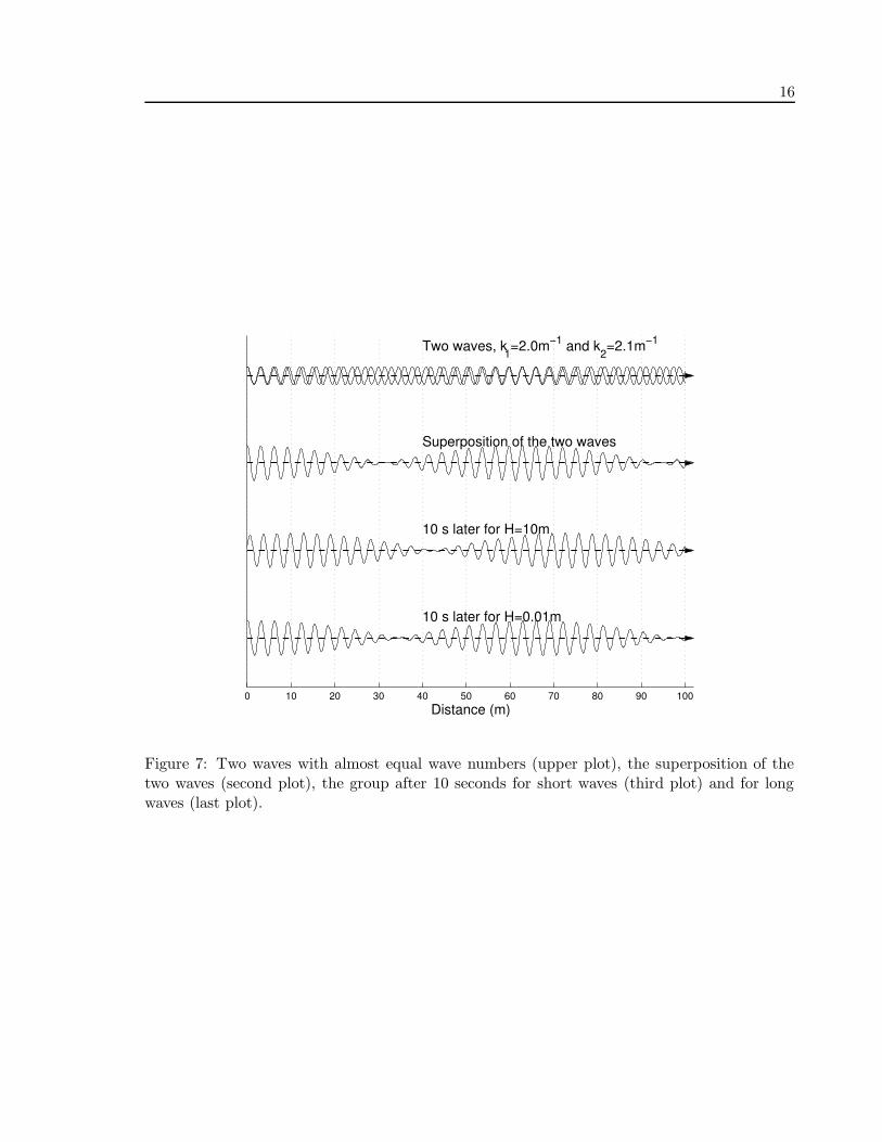
8a) We will look at two waves with almost equal wave numbers, k1 and k2 (see Figure 7).What are the corresponding frequencies ω1 and ω2 for a depth of 10 m (short waves) andfor a depth of 1 cm (long waves)?
8b) What are the phase velocities c of the two waves for the deep- and shallow water cases?
8c) Let k1 = k + δk, k2 = k − δk, ω1 = ω + δω, and ω2 = ω − δω, and show that thesuperposition of the two waves
η1 = η0 cos(k1x − ω1t), and η2 = η0 cos(k2x − ω2t)
can be writtenη = 2η0 cos(δkx − δωt) cos(kx − ωt).
What are the group velocities (cg) of the superposition of the two waves for the deep- andshallow water cases? How is the group velocity cg compared to the phase velocity c. Doyour results agree with Figure 7?
8d) Use the definition of the group velocity,
cg ≡ δω/δk
and the dispersion relationω2 = gk tanh(kH)
to derive the group velocity for short and long waves. What can you say about thedispersion properties of the two types of waves?
16
0 10 20 30 40 50 60 70 80 90 100
Two waves, k1=2.0m−1 and k2=2.1m−1
Superposition of the two waves
10 s later for H=10m
10 s later for H=0.01m
Distance (m)
Figure 7: Two waves with almost equal wave numbers (upper plot), the superposition of thetwo waves (second plot), the group after 10 seconds for short waves (third plot) and for longwaves (last plot).

17
9 Shallow water waves
We will now study the adjustment processes that take place when we have an initial disturbancyof the surface elevation. We will only consider waves that are long compared to depth. Forsimplicity, we look at the two-dimensional case, and neglect friction, non-linear terms, androtation.
9a) Start with the general equations of momentum and mass conservation and explain theassumptions we use to get the following set of equations
ρ∂u
∂t= −∂p
∂x, ρ
∂v
∂t= −∂p
∂y,
∂p
∂z+ ρg = 0, and
∂u
∂x+
∂v
∂y+
∂w
∂z= 0.
9b) We will now study waves with motion in the xz plane (v = 0 and ∂∂y = 0). Show that the
equations above can be written as the shallow water equations
∂u
∂t= −g
∂η
∂xand
∂η
∂t+ H
∂u
∂x= 0,
where η is surface elevation, g gravity and H the constant depth.
9c) Derive a single equation for η and seek a solution on the form η = η0 cos k(x − ct). Whatis the constant c? Are such waves dispersive?
9d) Show that the equation for the energy associated with this wave, is given by
∂
∂t(1
2ρHu2 +
1
2ρgη2) +
∂
∂x(ρgHuη) = 0.
Explain (using few words!) what the terms represent.
9e) Average over a wave length to show that the sum of the kinetic and the potential energyequals
E = Ek + Ep =1
2ρgη2
0 .
How is the energy divided between the kinetic (Ek) and the potential (Ep) forms?
9f) Consider the situation illustrated in Figure 8. Initially the fluid is at rest (u = 0) andthe surface elevation is given by η = G(x) where G(x) = η0 for −L ≤ x ≤ L and zeroelsewhere. Show that every functions on the form η = G1(x−ct)+G2(x+ct) are solutionsto the shallow water equations and calculate the velocity component u.
9g) Use the initial conditions to show that
G1(x) = G2(x) =1
2G(x),
and that the evolution with time is given by
η =
0 : |x − ct| > L and |x + ct| > Lη0 : |x − ct| < L and |x + ct| < L
η0/2 : otherwise
9h) Find the corresponding expressions for u and make a sketch of the surface elevation attimes ct = L/2 and ct = 3L/2.
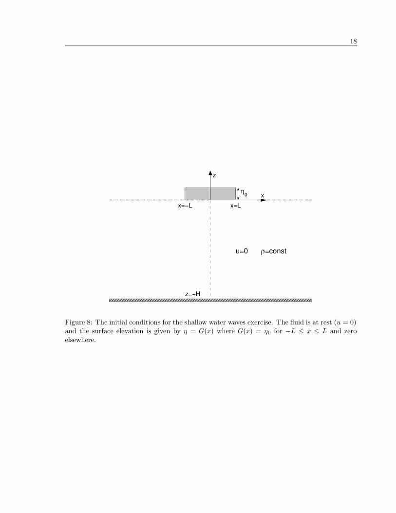
18
z
x
z=−H
x=−L x=L
η0
ρ=constu=0
Figure 8: The initial conditions for the shallow water waves exercise. The fluid is at rest (u = 0)and the surface elevation is given by η = G(x) where G(x) = η0 for −L ≤ x ≤ L and zeroelsewhere.

19
10 Tides in channels and bays
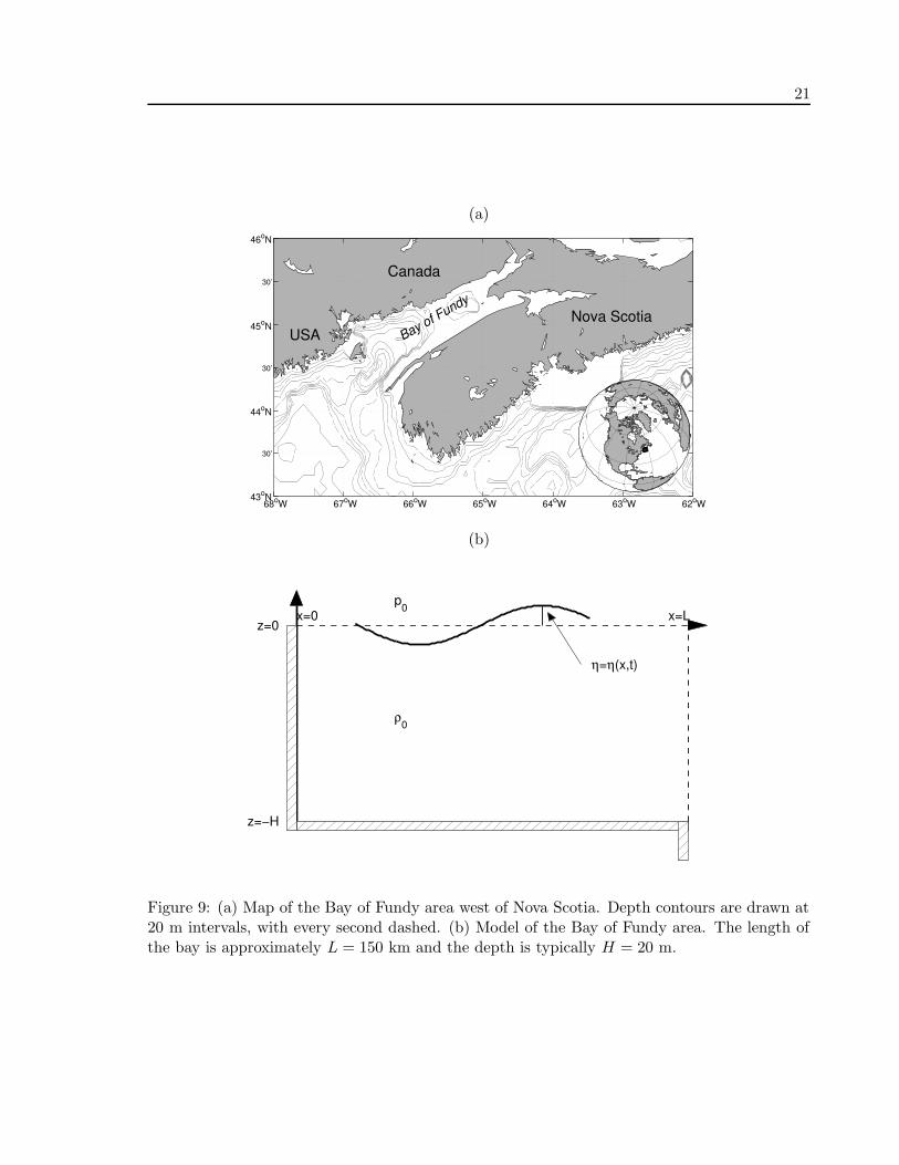
For narrow gulfs and channels, the propagation of tidal waves is to a good approximationdescribed by the shallow water equations. We will here look at a special case known as resonance.Resonance occurs when the forcing has a frequency that matches the frequency of one of thenatural modes of oscillations for the system. In certain areas, like the Bay of Fundy (see mapin Figure 9a), resonance effects make the tides become almost 10 meters in amplitude.
10a) We will model the Bay of Fundy system as a two-dimensional problem, with the coordinatesystem located at the head (inner end) of the bay, where we have a vertical wall, the mouthof the bay is located at x = L, and we assume constant air pressure, ocean density andocean depth. The governing equations for the problem may be written
∂u
∂t= −g
∂η
∂x, and
∂η
∂t+ H
∂u
∂x= 0,
where η is surface elevation and u the velocity component along the horizontal axis.Explain what simplifications we have made.
10b) A general wave solution of a wave propagating from the mouth of the bay towards it innerwall is η = η1 cos(kx + ωt). What is the relation between wave number k and frequencyω?
10c) A wave that has been reflected at the inner wall, will propagate out (towards right) givenby η = η2 cos(kx − ωt). Show that when η1 = η2 = η0/2, the superposition of the twowaves is given by
η = η0 cos kx cos ωt, and u =c
Hη0 sin kx sinωt,
where c is the phase speed c = ω/k.
10d) Now we will look at the boundary conditions at the open boundary. To avoid that thepressure gradient or the divergence are going towards infinity, both the perturbationpressure and mass (volume) transports must be continuous across the mouth of the bay.Show that this leads to a criteria for the impedance Z,
Z =ρgη
ρAu=
c
Acot kL cot ωt,
where cot = cos / sin is the cotangent function and A the area (width times height) at themouth of the bay.
10e) If we assume that the ocean just outside the bay is infinitely wide and deep compared tothe bay, Z = 0 outside the bay. Show that this implies that waves oscillating freely willhave distinct wave lengths and periods given by
λ =4L
2n + 1, and T =
4L√gH(2n + 1)
,
where n = 0, 1, 2, 3, ... is a counter. Make a sketch of the solution for the first three modes(n = 0, 1, 2).

20
10f) From the map in Figure 9a we estimate length L and depth H to be respectively 150 kmand 20 m. What are the period of the first three natural modes?
10g) Now we go back to the solution for the channel (in 10c) and assume that the tides producean oscillating surface elevation at the mouth of the bay given by ηT = ηF cosωF t, whereηF and ωF is amplitude and frequency of the forcing. Show that with this boundarycondition at the mouth of the bay, the equation for the surface elevation at the head ofthe bay becomes
η0 =ηF cos ωF t
cos kL cos ωt.
What happens if the frequency of the forcing approaches one of the natural frequenciesof the system, that is ωF ≈ ω?
10h) The period of the semi-diurnal (=twice a day) tides is 12.42 hours. Which of the firstthree modes found above does this period correspond to?
21
(a)
68oW 67oW 66oW 65oW 64oW 63oW 62oW 43oN
30’
44oN
30’
45oN
30’
46oN
USA
Canada
Nova ScotiaBay of Fundy
(b)
z=0
z=−H
ρ0
p0 x=Lx=0
η=η(x,t)
Figure 9: (a) Map of the Bay of Fundy area west of Nova Scotia. Depth contours are drawn at20 m intervals, with every second dashed. (b) Model of the Bay of Fundy area. The length ofthe bay is approximately L = 150 km and the depth is typically H = 20 m.

22
11 Internal waves
We will now turn our attention towards waves propagating on the boundary between fluidsof different densities. Ordinary surface waves van be viewed as internal waves, but as sincethe density difference between the ocean and atmosphere is very large (ρ0 ≈ 1000ρa), wetend to neglect the atmospheric density and the atmospheric motion set up by the waves, inthat particular kind of problems. Now we will investigate waves on an interface between twofluids, and where the density difference between the fluids are small. Examples may be wavespropagating on a boundary between fresh and more salty waters, or between warm air overlyingcold air (inversion)3.
11a) Give the linearised equations for long (hydrostatic) waves.
11b) Show that the horizontal velocities are independent of depth, and integrate the continuityequation over depth.
11c) We will now look at a model that consists of two, homogeneous, incompressible and fric-tionless layers with densities ρ1 and ρ2. The thickness of the two layers are H1 and H2
respectively, and the total depth is H = H1 + H2. The interface is perturbed vertically,given by h(x, t). We further use the rigid lid approximation. That means that we includethe pressure disturbances the wave at the interface will generate at the surface (the baro-clinic part), but ignore the velocities set up by any travelling waves at the surface (thebarotropic part). Thus the pressure at z = 0 will now depend on distance and time, thatis p0 = p0(x, t) (see Figure 10a). Find an expression for the pressures in the two layers,p1 and p2.
11d) Show that the equations for the horizontal velocity (momentum equation) in the twolayers become
∂u1
∂t= − 1
ρ1
∂p0
∂x, and
∂u2
∂t= − 1
ρ2
∂p0
∂x− g′
∂h
∂x,
where g′ = g(ρ2 − ρ1)/ρ2 is the reduced gravity.
11e) Integrate over each layer and linearise to show that the continuity equation gives
H1∂u1
∂x− ∂h
∂t= 0, and H2
∂u2
∂x+
∂h
∂t= 0.
11f) Combine the continuity equations with the momentum equations to find two expressionsfor ∂2h/∂2t, and by adding the two equations show that the equation for the disturbance(wave on the interface) becomes
∂2h
∂t2− c2
i
∂2h
∂x2= 0, where c2
i =ρ2H1H2
ρ1H2 + ρ2H1g′.
3This exercise is partly based on a master thesis by Birgitte Rugaard Furevik, ”Interne bølger i norske farvande
observert med ERS-1 SAR” published in 1995.

23
11g) Assume that the wave on the interface can be written h = h0 cos(kx − ωt), derive theexpressions for the horizontal velocity in the two layers, and show that
H1u1 + H2u2 = 0.
11h) Use the continuity equation and the linearised kinematic boundary condition at the in-terface (w1(−H1) = w2(−H1) ≈ ∂h/∂t) to derive the expressions for the vertical velocitycomponent in each the two layers,
w1 = −cih0k
H1z sin(kx − ωt), and w2 =
cih0k
H2(z + H) sin(kx − ωt).
11i) Make a sketch of the wave and the associated motion, and show where there is convergenceor divergence at the surface.
11j) In this exercise we used the long-wave approximations. Without this approximation, thecorresponding equation for the waves would have become slightly more complicated,
c2i =
g
k(ρ2 − ρ1)
tanh(kH1) tanh(kH2)
ρ1 tanh(kH2) + ρ2 tanh(kH1).
Show that the phase speed for long waves become the same as given above, and that theexpression for short waves may be written
c2i =
ρ2g′
k(ρ2 + ρ1).
Are these waves dispersive?
11k) If you look at the internal waves depicted in Figure 10b, can you use the long waveapproximation to explain what you see?
11l) What information would have been needed in order to find the area where these wavesare generated?

24
(a)
h=h(x,t)
z=0
z=−H1
z=−H
ρ1
ρ2
P0(x,t)
(b)
Figure 10: (a) A simple model of a two-layer system with an fixed ice cover on top. (b) Asynthetic aperture radar (SAR) image taken from the European ERS1 satellite. The imageis from the Mediterranean side of the Strait of Gibraltar (Spain and Gibraltar is the upperleft area, and Morocco the lower left area), and covers roughly 60 km × 40 km. The SARmeasures the roughness of the surface, which is essentially the small surface ripples of a fewcentimetres. Where the surface water is converging, the ripples become steeper which is seen asbright areas in the image. Opposite, where the surface water is diverging, the ripples becomesmoother, which is detected as darker areas. Note the internal waves propagating eastwardfrom the strait. The dark winding line is due to oil release from a boat, which destroys thesurface tension and the ripples can not develop.
25
12 A floating bridge
Again we look at a two-layer system. However, this time we will look at the combined effect ofa barotropic (surface) wave and a baroclinic (internal) wave4.
12a) In a fjord the tidal wave will have the form of a progressive wave, where the surfaceelevation is given by η = η0 sin(k0x−ωt), and the total depth is H. Use the shallow waterequations to find the corresponding barotropic velocity u0, and express the wave numberk0 in terms of the frequency ω, which for the tidal wave is a known constant.
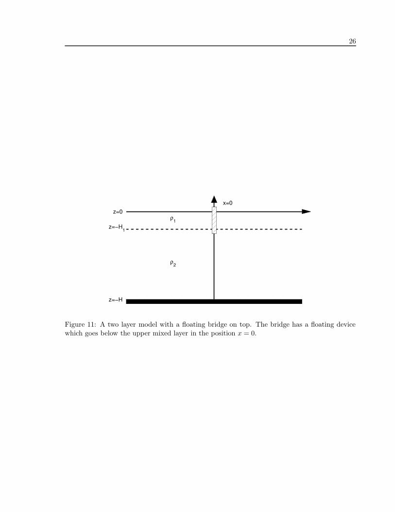
12b) The fjord has a upper layer of thickness H1 and density ρ1, and a lower layer of thicknessH2 and density ρ2. Across the fjord there is going to be built a floating bridge, where thedepth of each of the floating pontoons is reaching below the mixed layer, that is below theinterface between the light surface water and the denser deep water (see Figure 11). Weassume that the barotropic wave can continue without being affected by the pontoon (thisis a good approximation if the upper layer is shallow compared to the total depth), butthat the bridge sets up internal progressive waves on each side of the bridge. We assumethat the horizontal velocities of the internal waves on each side is given by
u1 = A sin(k1x + ωt) for x < 0, and u1 = B sin(k1x − ωt) for x > 0.
Integrate the equation of continuity over the upper layer, and find an expression for thedisplacement h of the interface.
12c) Integrate the equation of continuity over the lower layer, and show that the horizontalvelocity in the lower layer becomes
u2 = −H1
H2u1.
12d) Use rigid lid approximation to express the wave number for the waves at the interface k1
in terms of ω Suggestion: Use the results you found in part f) in the previous exercise.
12e) A boundary condition is that the total velocity, which is the sum of the barotropic velocity(u0) and the upper layer velocity associated with the internal wave (u1) is zero at x = 0.Physically u = u0 + u1 = 0 at x = 0, means that there is no flow through the pontoon.Use this boundary condition to determine the strength of the internal wave, show that
A =ωη0
k0H, and B = − ωη0
k0H,
and find the corresponding expressions for the amplitude of the interface displacement.
12f) Use the values η0 = 1 m, H1 = 5 m, H2 = 100 m, ρ1 = 1020 kgm−3, ρ2 = 1030 kgm−3,and ω = 1.3× 10⁻⁴ s−1, and estimate the wave numbers k0 and k1 (or wave lengths), andthe amplitude of the interface displacement h. Make a sketch of the wave.
4This exercise is modified from exercises in GFO210 by Martin Mork and Frank Nilsen.
26
z=0
z=−H1
z=−H
ρ1
ρ2
x=0
Figure 11: A two layer model with a floating bridge on top. The bridge has a floating devicewhich goes below the upper mixed layer in the position x = 0.
27
13 Internal waves in a continuously stratified fluid
Internal waves can always be present in a stratified fluid, even without a discontinuity in density.In this exercise we will therefore study waves in a continuous, stratified, incompressible fluid.
13a) We will look at a situation where the density and pressure is close to their mean depth-depending values, that is ρ = ρ0(z)+ρ′(x, y, z, t) and p = p0(z)+ p′(x, y, z, t), where ρ′ ρ0 and p′ p0. Show that the Boussinesq approximation together with the assumptionof incompressibility give the following five equations to describe the motion in the fluid
ρ0∂u
∂t= −∂p′
∂x, (1)
ρ0∂v
∂t= −∂p′
∂y, (2)
ρ0∂w
∂t= −∂p′
∂z− ρ′g, (3)
∂ρ′
∂t+ w
dρ0
dz= 0, (4)
∂u
∂x+
∂v
∂y+
∂w
∂z= 0. (5)
13b) Combine equations (1) and (2) with (5), and (3) with (4), to find the following twoequations for the relationship between the vertical velocity and the pressure perturbations
ρ0∂2w
∂z∂t=
∂2p′
∂x2+
∂2p′
∂y2, (6)
ρ0∂2w
∂t2= − ∂2p′
∂t∂z− ρ0N
2w, (7)
where N 2 = − gρ0
dρ0
dz . What is the name of the parameter N and what is its physicalmeaning?
13c) Differentiate equation (6) with respect to z and t, (7) twice with respect to x, and (7)twice with respect to y, assume that the vertical variation in ρ0 is much less than thevertical variations in w, and show that a single equation for the vertical velocity is
∂2
∂t2∇2w + N2∇2
Hw = 0, (8)
where ∇2 = ∂2
∂x2 + ∂2
∂y2 + ∂2
∂z2 and ∇2H = ∂2
∂x2 + ∂2
∂y2 .
13d) Assume a wave component on the form w = w0 cos(kx + ly + mz − ωt) to derive thedispersion relation for internal waves in a continuous stratified fluid.
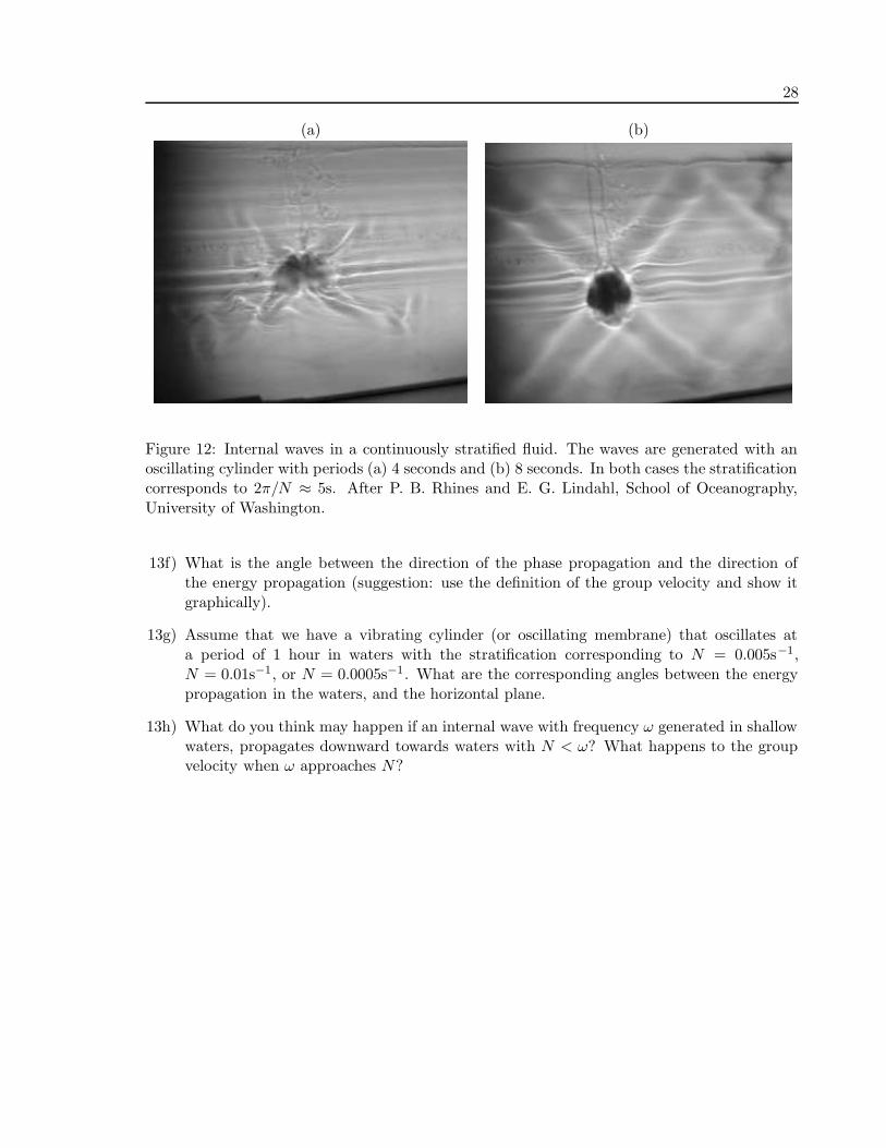
13e) Show that the frequency only depends on the stratification and the angle between the wavenumber vector and the horizontal plane, ω = N cosφ (see Figure 12). Explain what youare seeing in the figure. Give a physical explanation for why the frequency should dependon the direction of the wave propagation, and what are the reasons for the frequency tobe between 0 and N?
28
(a) (b)
Figure 12: Internal waves in a continuously stratified fluid. The waves are generated with anoscillating cylinder with periods (a) 4 seconds and (b) 8 seconds. In both cases the stratificationcorresponds to 2π/N ≈ 5s. After P. B. Rhines and E. G. Lindahl, School of Oceanography,University of Washington.
13f) What is the angle between the direction of the phase propagation and the direction ofthe energy propagation (suggestion: use the definition of the group velocity and show itgraphically).
13g) Assume that we have a vibrating cylinder (or oscillating membrane) that oscillates ata period of 1 hour in waters with the stratification corresponding to N = 0.005s−1,N = 0.01s−1, or N = 0.0005s−1. What are the corresponding angles between the energypropagation in the waters, and the horizontal plane.
13h) What do you think may happen if an internal wave with frequency ω generated in shallowwaters, propagates downward towards waters with N < ω? What happens to the groupvelocity when ω approaches N?
29
14 Lee waves
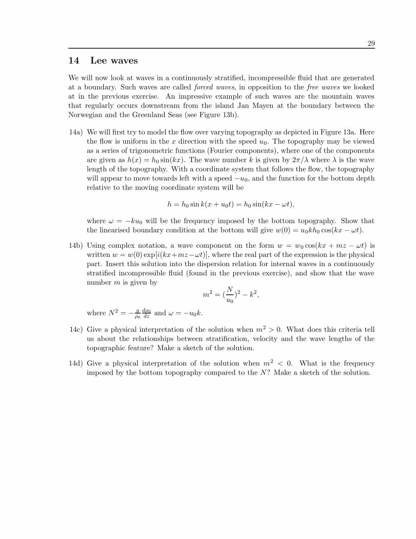
We will now look at waves in a continuously stratified, incompressible fluid that are generatedat a boundary. Such waves are called forced waves, in opposition to the free waves we lookedat in the previous exercise. An impressive example of such waves are the mountain wavesthat regularly occurs downstream from the island Jan Mayen at the boundary between theNorwegian and the Greenland Seas (see Figure 13b).
14a) We will first try to model the flow over varying topography as depicted in Figure 13a. Herethe flow is uniform in the x direction with the speed u0. The topography may be viewedas a series of trigonometric functions (Fourier components), where one of the componentsare given as h(x) = h0 sin(kx). The wave number k is given by 2π/λ where λ is the wavelength of the topography. With a coordinate system that follows the flow, the topographywill appear to move towards left with a speed −u0, and the function for the bottom depthrelative to the moving coordinate system will be
h = h0 sink(x + u0t) = h0 sin(kx − ωt),
where ω = −ku0 will be the frequency imposed by the bottom topography. Show thatthe linearised boundary condition at the bottom will give w(0) = u0kh0 cos(kx − ωt).
14b) Using complex notation, a wave component on the form w = w0 cos(kx + mz − ωt) iswritten w = w(0) exp[i(kx+mz−ωt)], where the real part of the expression is the physicalpart. Insert this solution into the dispersion relation for internal waves in a continuouslystratified incompressible fluid (found in the previous exercise), and show that the wavenumber m is given by
m2 = (N
u0)2 − k2,
where N 2 = − gρ0
dρ0
dz and ω = −u0k.
14c) Give a physical interpretation of the solution when m2 > 0. What does this criteria tellus about the relationships between stratification, velocity and the wave lengths of thetopographic feature? Make a sketch of the solution.
14d) Give a physical interpretation of the solution when m2 < 0. What is the frequencyimposed by the bottom topography compared to the N? Make a sketch of the solution.

30
(a)
zx
u0
h=h(x)
(b) (c)
Figure 13: (a) Model of a uniform flow of speed u0 over a mountain where amplitude of a Fouriercomponent of the topography is h. (b) Satellite picture of a mountain wave cloud patterns inthe wake of Jan Mayen on 25th of January 2000. The wind is blowing from southwest, which isfrom the upper left corner of the satellite picture in (b). Note how the waves penetrate hundredsof kilometres downstream of Mount Beerenberg at Jan Mayen, where it is generated.
31
15 Normal modes
The ocean and the atmosphere are thin sheets of fluid in the sense that their horizontal scalesare much larger than the depth or height scales. Also most of the energy associated with motionlies in components with horizontal scales much larger than the vertical. For such motions we canuse the hydrostatic approximation. In this exercise we will also introduce a common techniqueknown as separation of variables.
We will here study an example with a tidal flow entering a basin at an open boundary,setting up motion in a continuously stratified fluid (see Figure 14)5.
15a) We assume that we have a continously stratified, incompressible fluid in a non-rotatingframe, and that we have only motion in the (x, z)-plane. Use Boussinesq and hydrostaticapproximations and set up the four linearized equations that determine the flow.
15b) Show by elimination that two equations relating perturbation pressure p ′ and verticalvelocity w are
ρ0∂2w
∂z∂t=
∂2p′
∂x2and ρ0N
2w = − ∂2p′
∂t∂z,
where N 2 = − gρ0
dρ0
dz . What is the physical interpretation of N?
15c) Combine the two equations above to derive one equation for the vertical velocity,
∂2
∂t2
[
∂
∂z(ρ0
∂w
∂z)
]
+ ρ0N2 ∂2w
∂x2= 0.
15d) Assume a solution on the formw = w(x, t)φ(z),
and show that a necessary consequence is
∂2w∂t2
∂2w∂x2
=−ρ0N
2φ∂∂z (ρ0
∂φ∂z )
= c2,
where c is a constant. Explain why the general solution for w becomes
w(x, t) = F (x − ct) + G(x + ct).
What is the physical interpretation of the constant c?
15e) Show that the boundary condition at the bottom gives
φ(−H) = 0,
and that the boundary conditions at the free surface together with the first equation underb) gives
ρ0∂3w
∂t2∂z− gρ0
∂2w
∂x2= 0 at z = 0,
and thusdφ
dz− g
c2φ = 0 at z = 0.
5This exercise is modified from exercises in GFO210 by Martin Mork and Frank Nilsen.
32
15f) Use the results under d) to show that the equation for φ becomes
∂
∂z(ρ0
∂φ
∂z) + ρ0(
N
c)2φ = 0,
and explain why this to a very good approximation can be written
∂2φ
∂z2+ (
N
c)2φ = 0.
15g) Together with the boundary conditions in e), the equation for φ above forms a so-calledSturm-Liouville problem. As we will see, these kind of problems will give an infinitenumber of solutions for c, so-called eigenvalues, and for each eigenvalue, there will be asolution for φ, which is known as the eigenfunction. A general solution for this problemis
φ = C sinκ(z + γ),
where C is the constant amplitude, and κ and γ are constants to be determined. Showthat κ = N/c and γ = H, and use the surface boundary condition to show that anequation for c is given by
tanNH
c=
N2H/g
NH/c.
15h) Show that for small values of the argument for the tan function above, the phase speed isgiven by c2 = c2
0 ≈ gH, and that for larger values of the argument, c = cn ≈ NHnπ , where
n = 1, 2, 3, .... Suggestion: Make a sketch of the tan x and 1/x functions an show wherethe curves cross.
15i) Show that the phase speed of the barotropic mode (c0) in h) corresponds to the homoge-neous case with N = 0, and that the phase speeds for the baroclinic modes can be foundby using the rigid lid approximation w(0) = 0. Make a sketch showing how the verticalvelocity of the barotropic and the first 3 baroclinic modes depend on depth.
15j) Measurements show that the density profile is given by
ρ0 = ρ
(
1 − εz
H
)
,
where ρ is the mean density, ε = 0.001, and H = 1000m. Calculate the phase speeds forthe barotropic and the first 3 baroclinic modes.
15k) Explain why the general solution can be written
w =n=∞∑
n=0
Cn sinκn(z + H)[F (x − ct) + G(x + ct)].
In order to determine the amplitudes of each of the modes, the constants Cn, we mustuse the boundary conditions. Use the equation of continuity to show that the horizontalvelocity must be on the form
u =n=∞∑
n=0
un(x, t)d
dz[φn(z)] ,

33
where∂
∂xun = −wn.
15l) Use the simplified equation for φ (under f) to show that each of the eigenfunctions for uare orthogonal to each other, that is
∫ z=0
z=−H
dφn
dz
dφm
dzdz = 0, for n 6= m.
Suggestion: Write the equation in f as c2nd2φn/d2z + N2φn = 0, do the same for a com-
ponent φn, multiply the two equations with dφm/dz and dφn/dz respectively, subtract andintergrate.
15m) At a location x = 0 a tidal current on the form u0 = U(z) cos ωt is measured. Assumethat U(z) can be written on the form
U(z) =n=∞∑
n=0
Andφn
dz,
and show that the constants An are given by
An =
∫ z=0z=−H U(z)dφn
dz dz∫ z=0z=−H(dφn
dz )2 dz.
15n) Show that with U(z) = U0 = constant and H1 = H/2, the values for the An’s become
An =−2U0H sin[nπ
H (H − H1)]
(nπ)2,
and U(z) becomes
U(z) = −2U0
n=∞∑
n=0
sin nπ2
nπcos
nπ
2(z + H)
= −2U0H(1
π
dφ1
dz+
1
9π
dφ3
dz+
1
25π
dφ5
dz+ ... +
1
n2π
dφn
dz).
15o) The assumed solution fits with a tidal current over a sill. For x > 0 the solution becomes
u =n=∞∑
n=0
Andφ
dzcosω(t − x
cn).
Find the corresponding expression for the vertical velocity w and the maximum verticaldisplacement associated with each of the modes. With a tidal current of U(z) = 0.1ms−1
at the inflowing boundary x = 0, what are the maximum displacements associated witheach of the first three modes?

34
zx
u0(z,t)
η=η(x,t)
N2=const
depth=H1 depth=H
Figure 14: Model of a basin with a flow entering at an open boundary. The open boundary islocated at x =, and the flow here is given by u0(z, t). The depth of the inflow is H1 and totaldepth H. The density is increasing linearly with depth, given a constant buoyancy frequencyN .

35
16 Geostrophic adjustment in a two-layer fluid
We are going to look at a simple model for geostrophic adjustment. We assume an infinitelydeep ocean, where the density in the surface in one part of the ocean is reduced due to awarming or a freshening. The density anomaly reaches down to a depth H1. Initially, we have atwo-layer system where everything is at rest (u = v = 0), and where the thickness of the upperlayer is given by h = H1 for x < 0, and h = 0 for x > 0. The density in the two layers are ρ1
and ρ2. There is no variations in the y direction, so we have ∂∂y = 0 everywhere in the fluid6.
16a) The equations for the motion in the upper layer, is almost the same as those given in theprevious exercise, with the exception that ∂
∂y = 0, ρ is replaced by ρ1, and we keep thenon-linear terms since the perturbation of the interphase is large (it goes to the surface).
∂u
∂t+ u
∂u
∂x− fv = − 1
ρ1
∂p
∂x(1)
∂v
∂t+ u
∂v
∂x+ fu = 0 (2)
∂p
∂z= −ρg (3)
∂u
∂x+
∂w
∂z= 0, (4)
Now using the assumption of a motionless abyss (∇p = 0 in the lower layer), show thatthe pressure term can be written − 1
ρ1
∂p∂x = −g′ ∂h
∂x , where g′ = ρ2−ρ1
ρ2is the reduced gravity.
Integrate the continuity equation over the upper layer, and show that the three equationsthat describe the system are:
∂u
∂t+ u
∂u
∂x− fv = −g′
∂h
∂x(5)
∂v
∂t+ u
∂v
∂x+ fu = 0 (6)
∂h
∂t+
∂
∂x(hu) = 0 (7)
16b) Due to the non linear terms (u ∂u∂x , u ∂v
∂x and hu), the equations above are impossible tosolve analytical. However, much can be said about the state of the fluid when the flowhas become stationary. After the adjustment process, the equation of continuity (7) yields∂∂x(hu) = 0, thus hu must be a constant. Since h = 0 at some points, the constant must bezero. But, as h 6= 0 at other points, it follows that u = 0 everywhere after the adjustment.Use this argument to show that the velocity after the adjustment is given by
v =g′
f
∂h
∂x. (8)
16c) All flows that are in geostrophic balance are solutions to the equation above. In orderto find an exact solution, we must use our most powerful tool, that is the conservation
6This exercise is mainly from Benoit Cushman-Roisin: Introduction to geophysical fluid dynamics.
36
of vorticity. Differentiate equation (6) to show that the time evolution of the relativevorticity of the flow is
Dζ
Dt+ (ζ + f)
∂u
∂x= 0, where ζ =
∂v
∂x(9)
(remember that ∂∂y = 0), and use equation (7) to substitute for the divergence of the flow
to get a single equation for the conservation of the potential vorticity of the fluid,
D
Dt(ζ + f
h) = 0. (10)
Thus the property (ζ+f)/h will be a conserved property of the motion, and from knowingthe initial conditions, we are able to derive information for the final state of the flow,
∂v∂x + f
h=
f
H1. (11)
16d) Despite the non-linearity of the original equations, we now have two perfectly linearequations that gives the relationship between velocity v and thickness of the upper layerh, that is equations (8) and (11). Combine the two to get a single equation for thethickness of the upper layer h, and show that the solution may be written
h = H1(1 − exp(x − x0
a), and v = −
√
g′H1 exp(x − x0
a) (12)
where a =√
g′H1/f is known as the internal (or baroclinic) Rossby radius of deforma-tion, and x0 is the position where the interface reaches the surface (where the isopycnaloutcrops).
16e) In order to determine the constant x0, we use conservation of water masses. To conservethe volume (remember that travelling waves do not transport water), the ”loss” of surfacewater from the left hand side of the x = 0 line, must equal the ”gain” at the other side.Thus
∫ 0
−∞
(H1 − h)dx =
∫ x0
0hdx. (13)
Show that the constant is given by x0 = a. Can you with few words describe the physicsthat gives this migration of the interface?
16f) It is rather straight-forward to calculate the energy of the system at the initial state (onlypotential energy) and at the final state (potential and kinetic energy). From initial to finalstage there is a loss in potential energy given by ∆PE = 1
4g′H21a and a gain in kinetic
energy of ∆KE = 112g′H2
1a. Thus the system has ”lost” 2/3 of the total energy (potential+ kinetic) from the initial state to the final state. Can you explain where the energy hasgone?

37
(a)
z=0
z=−H
ρ2
x=0
Heating
(b)
z=0
z=−H1
z=−H
ρ1
ρ2
x=0
(c)
z=0
z=−H1
z=−H
ρ1
ρ2
x=0
h=h(x)
Figure 15: An illustration of a geostrophic adjustment in a two layer case. In (a), atmosphericheating (or precipitation) reduce the density of the upper layer of the ocean for x < 0, whilethe upper ocean for x > 0 remains at the same density as the lower ocean. The result is a twolayer system in one part of the domain, and a one-layer system in the rest of the domain, asillustrated in (b). In the upper part of the ocean, the water masses are separated by a sharpfront. After geostrophic adjustment, the front between the two water masses will be slopingfrom the surface towards its initial depth.

38
17 Long waves in a fluid that is rotating
For fluid motion (waves) that evolves on a time scale comparable to or longer than the timescale of the rotation of the Earth (1 day), the Coriolis acceleration must be included in theequation of motion. Here some of the effects of the rotation will be explored.
17a) In its general form the equation of motion is
Du
Dt+ 2Ω × u = −1
ρ∇p − g + ν∇2u. (1)
Explain what the different terms in the equation represent.
17b) We now linerize the equation, neglect friction, assume hydrostatic balance and a non-divergent flow, and finally assume that horizontal scales are much larger than the verticalscales (w u, v). Show that the equations that governs the motion become
∂u
∂t− fv = −1
ρ
∂p
∂x(2)
∂v
∂t+ fu = −1
ρ
∂p
∂y(3)
∂p
∂z= −ρg (4)
∂u
∂x+
∂v
∂y+
∂w
∂z= 0, (5)
where f = 2Ω sinφ, with Ω being the rotation rate of the Earth and φ the latitude.
17c) Assume constant density, and show that the equations can be written
∂u
∂t− fv = −g
∂η
∂x(6)
∂v
∂t+ fu = −g
∂η
∂y(7)
∂η
∂t+ H(
∂u
∂x+
∂v
∂y) = 0. (8)
Which of the terms in equations (6) and (7) will dominate if the motion evolve on a timescale that is (a) much larger than, (b) comparable to, or (c) much less than the rotationperiod of the Earth?
17d) We will now derive a single wave equation for the surface elevation η. Differentiate equa-tions (6) and (7) and combine to find a single equation for the time evolution of thedivergence of the velocity field. Combine this with equation (8) to show that an equationfor the surface elevation may be written
∂2η
∂t2− c2∇2
Hη + fHζ = 0, (9)
where c =√
gH is the wave speed for shallow water waves without rotation and ζ = ∂v∂x−∂u
∂yis the relative vorticity.

39
17e) Differentiate equations (6) and (7) and combine to find a single equation for the timeevolution of the relative vorticity of the field. Combine this with equation (8) to showthat the equation for the time evolution of the relative vorticity is ∂ζ
∂t = fH
∂η∂t , and combine
with equation (9) to get the single equation for the surface elevation,
∂
∂t(∂2η
∂t2− c2∇2
Hη + f2η) = 0. (10)
17f) Assume that the surface elevation has the form of a travelling wave, and show that thedispersion relation gives the solutions
ω = 0, or ω2 = f2 + c2(k2 + l2). (11)
What is the physical interpretation of ω = 0?
17g) Make a sketch of the solution (for instance of w/f as a function of wave number). Discussthe solution above for the case when the waves become very small (but still large enoughfor the hydrostatic approximation to be valid), and for the case when the waves becomevery large. What is the group velocity for the two cases?
40
18 Tsunami
When two continental plates collide, this often leads to an earthquake and a sudden verticaldisplacement of one of the plates. When this happens on the bottom of the ocean, it leadsto a sudden difference in the sea-level and tsunami waves are radiating from the centre of theearthquake. The tsunami killing 300 000 people in the Indian Ocean 26th of December 2004is an example of how devastating such waves can be. We will study the adjustment processestowards equilibrium after such a vertical displacement on the sea floor, and assume that thesurface elevation just after the displacement is given by η = η0sgn(x), where sgn(x) = −1 whenx < 0 and 1 when x > 07.
18a) Explain what assumptions we are using to arrive at the following set of equations:
∂u
∂t− fv = −g
∂η
∂x∂v
∂t+ fu = −g
∂η
∂y
∂η
∂t+ H(
∂u
∂x+
∂v
∂y) = 0.
18b) Combine the equations and show that the wave equation for the surface elevation can bewritten as
∂2η
∂t2− c2(
∂2η
∂x2+
∂2η
∂y2) + fHζ = 0.
Write down the expressions for c and ζ and give a brief physical explanation for each.
18c) Show that ζ/f − η/H is constant with time, and that the wave equation thus may bewritten
∂2η
∂t2− c2(
∂2η
∂x2+
∂2η
∂y2) + f2η = f2η0sgn(x).
18d) In order to study what kind of waves the discontinuity in the surface elevation sets up, wefirst look at the homogeneous part of the equation above (i. e. the right hand side is setto zero). Assume a solution on the form η = η0 cos(kx + ly − ωt) (or use complex form ifyou wish), and show that the dispersion relation is given by
ω2 = f2 + (k2 + l2)c2.
18e) Make a sketch that shows how the frequency depends on the wave number, and discussthe phase- and group velocities for very short and very long waves. What happens tothe frequency when the wave length goes towards infinity, and what is the name of suchwaves?
18f) We will now look at the stationary part of the wave equation given in c. As the initialcondition is independent of y, we may assume that the solution will be independent of y
7This exercise was given at the GEOF330 exam 8. December 2004.

41
at all times. Solve for η and v and use the boundary condition that both are continuousin x = 0 to show that the surface elevation is given by
η = η0(1 − e−x/a) for x > 0, and η = η0(−1 + ex/a) for x < 0.
What is the expression for a and what is the name of this parameter?
18g) If we calculate the change in potential and kinetic energy from the initial state to thefinal equilibrium state, we find that only one third of the released potential energy hasbeen used to increase the kinetic energy of the system. Can you comment on this? Whatis special with adjustment to equilibrium in rotating systems compared to non-rotatingsystems?

42
19 Thermal wind I: The Denmark Strait overflow
For large scale flow in the atmosphere and ocean, the motion is generally close to geostrophicbalance, that is there is a simple balance between the Coriolis and the pressure terms. Ifthe velocity is measured at a certain height or depth, and we have information of the densitystructure in the atmosphere or in the ocean, it is possible to find the velocity at all levels usingthe thermal wind equations. This is the topic for the following exercise.
19a) Start with the geostrophic balance and derive the thermal wind equations for the verticalvelocity shear in the x and y directions,
∂u
∂z=
g
ρ0f
∂ρ
∂y, and
∂v
∂z= − g
ρ0f
∂ρ
∂x. (1)
19b) In the case of a pronounced density contrast (strong pycnocline), a two layer system maybe applicable. Show that in this case the thermal wind equation for the north-southvelocity component may be written
v1 − v2 = − g
ρ0f(ρ2 − ρ1)
δz
δx, (2)
where subscripts 1 and 2 refer to the upper and lower layers, and δz/δx will be the slopeof the interphase between the two layers (suggestion: discretize the derivatives in theequation for the vertical velcity shear in the y direction, and multiply with δz).
19c) Measurements from the strait between Greenland and Iceland (Denmark Strait) show adensity profile that to a good approximation can be described as a 3-layer system, asshown in Figure 16. We first assume that there is no flow in the middle layer in the strait,and use the values g = 10 ms−2, ρ0 = 103 kgm−3, and f = 10−4 s−1. Calculate thevelocities in the two other layers, and make a sketch of the results.
19d) From other measurements we know that the total transport through the strait is 6 × 10⁶
m3s−1. What is the velocity in the middle layer assuming that it is the same everywherein that layer?
19e) Use the results above to make a sketch of the surface topography. What is the differencein the sea surface height between Iceland and Greenland?

43
0 20 40 60 80 100 120 140 160
0
100
200
300
400
500
600
700
800
900
1000
ρ1=1027.0
ρ2=1027.5
ρ3=1028.0Greenland Iceland
Distance (km)
Dept
h (m
)
Figure 16: Density distribution in the Denmark Strait between Greenland and Iceland.

44
20 Thermal wind II: The Norwegian Coastal Current
In Figure 17 we have shown the distribution of temperature, salinity, and potential density ina section going from Svinøy (just north of Stadt at the west coast of Norway) and towardsnorthwest. From the observations taken in March we can recognize the relatively warm andsaline waters of the Norwegian Atlantic Current over the deepest parts of the section, andthe cold and fresh waters of the Norwegian Coastal Current over the more shallow continentalshelf8.
20a) Start with the general form of the equation of motion, and show which assumptions thatare made in the geostrophic approximation,
−fv = −1
ρ
∂p
∂x, fu = −1
ρ
∂p
∂y, and − ∂p
∂z− ρg = 0. (1)
20b) Let the x axis be directed eastward towards the coast in Figure 17, and the y axis pointnorthward into the section, and show that the vertical derivative of the northward flow isgiven by
∂v
∂z= − g
ρ0f
∂ρ
∂x,
where ρ0 is a reference density (Boussinesq approximation).
20c) Give a rough estimate of the difference in velocity between the surface and the 200mdepth at station 280 (Figure 17). In which parts of the section do we have the strongestbaroclinicity?
20d) In order to get an estimate of the volume transport of the Norwegian Coastal Current,we simplify the density structure to a two-layer system with constant density (ρ1 andρ2) in each layer. We choose the interphase between the two layers to be defined by theσt = 27.2 isopycnal, and assume that the upper layer is in geostrophic balance and thatthe lower layer is at rest. The coast we simplify to a vertical wall at the position x = 0.The total depth of the upper layer is H = η+h where η is the height of the surface (z = η)and h the depth of the interphase (z = −h). Make a sketch of the situation and find thepressure in each of the two layers expressed by η and h.
20e) Use that the lower layer is motionless to find a relation between the displacement of thesurface elevation and the thickness of the upper layer.
20f) Show that the current in the upper layer is given by
v =g′
f
∂H
∂x,
where g′ = g(ρ2 − ρ1)/ρ2 is the reduced gravity.
20g) Show that the volume transport in the upper layer becomes
V =g′
2fH2
0 ,
where H0 is the thickness of the upper layer at the coast (in x = 0).
8This exercise was given at the GEOF110 exam 15. December 2003.

45
20h) From Figure 17 find suitable values for ρ1, ρ2, and layer thickness H0 and find the surfaceelevation at the coast and the total volume transport in the flow.
20i) In this model many approximations have been used. Mention the two you believe willhave the largest impacts on your answers in h).

46
Figure 17: Measurements of temperature (upper panel), salinity (middle panel), and potentialdensity (lower panel) from the Svinøy section 30. March 1978. The depth is given in meters,and the horizontal length scale is given in the lower panel (20 nm = 37 km). The numbersabove each plot refer to the station numbers where the measurements are taken.
47
21 Available potential energy
If the surface and all internal surfaces of constant density are flat, there will be no horizontalpressure gradients in a fluid. In that case there is no potential energy in the fluid that canbe converted to kinetic energy, and we say that the available potential energy (APE) is zero.If, however, there are internal density gradients, a relaxation of the wind field or flow that iscausing the pressure gradients will always lead to a conversion of energy from the potential tothe kinetic forms. Thus some of the APE will be released. In this exercise we will study theconcept of APE, and also a case with a conversion from kinetic to potential energy.
21a) Calculate the potential energy for the two cases (a) and (b) in Figure 18 and show thatthe available potential energy in (a) is given by
1
12(ρ2 − ρ1)gH2L.
21b) Due to conservation of mass, the constant density in Figure 18d must be the same as themean density in (c), that is ρ = 0.5(ρ1 + ρ2). What is the increase in potential energyfrom (c) to (d). Is the APE increasing? Compare with (a) and explain the answer.
21c) We have earlier discussed adjustment towards equilibrium for a case without (Fig 5.9 inGill and exercise 9) and with (Fig 7.3 in Gill) rotation. What can you say about thefraction of the APE that is converted to kinetic energy in the two cases?
21d) Due to continuity (and conservation of momentum in absence of other external forcings),the vertical integrated flow in Figure 18d must be the same as it is in (c), that is u =0.5(u1+u2). It is clear that the energy used to increase the potential energy from Figure 18cto (d) must come from the change in kinetic energy. Show that complete vertical mixingis only possible if
(ρ2 − ρ1)gH
ρ0(u2 − u1)2<
1
2,
where we have applied the Boussinesq approximation when calculating the kinetic en-ergy (ρ1 ≈ ρ2 ≈ ρ0). Discuss the physical meaning of this result (in terms of densitystratification and velocity shear).

48
(a)
0 L
H
ρ=ρ1+(ρ2−ρ1)x/L
(b)
0 L
H
ρ=ρ2+(ρ1−ρ2)z/H
(c)
0 L
H
ρ=ρ2+(ρ1−ρ2)z/Hu=u1+(u2−u1)z/H
(d)
0 L
H
ρ=0.5*(ρ1+ρ2)u=0.5*(u1+u2)
Figure 18: Different configurations of a density field in a fluid of width L and height H. In(a) the density is increasing towards right, and in (b) it is increasing with depth. The lattersituation is also shown in (c) where we also put on a depth-dependent flow u. If the shear ofthe flow is large, vertical instabilities may occur, leading to a strong mixing of the fluid and thesituation shown in (d).

49
22 Vorticity dynamics
In this section we will derive one of the most powerful tools in geophysical fluid dynamics,namely the equation for the conservation of potential vorticity. This equation will then beused to estimate the changes in a flow along a coast, when the water depth changes in thealong-stream direction9.
22a) With the non-linear terms included, the shallow water equations are
Du
Dt− fv = −g
∂η
∂x(1)
Dv
Dt+ fu = −g
∂η
∂y(2)
D
Dt(η + H) + (η + H)(
∂u
∂x+
∂v
∂y) = 0, (3)
where u and v are the two horizontal velocity components, η the surface elevation, H =H(x, y) the bottom depth, f = f(y) the Coriolis parameter, g the gravity, and the operator
D
Dt≡ ∂
∂t+ u
∂
∂x+ v
∂
∂y.
Show that the change in the absolute vorticity becomes
D
Dt(f + ζ) + (f + ζ)(
∂u
∂x+
∂v
∂y) = 0, (4)
where ζ = ∂v∂x − ∂u
∂y is the relative vorticity. Explain with words what will happen if thereis divergence or convergence in the horizontal flow?
22b) Combine with the equation of continuity to show that the conservation of potential vor-ticity is given by
D
Dt(f + ζ
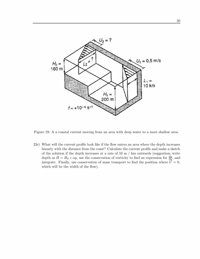
H + η) = 0. (5)
We will now investigate a coastal current as it moves from an area with deep water to amore shallow area (Figure 19). Current maximum is at the coast and it decreases linearlyto 0 (zero) at a distance L1 from the coast. In the deep area the current at the coastis U1 =0.5 ms−1, the width of the current L1 =10 km, and the water depth is 200 m.The Coriolis parameter is f = 10−4 s−1. Calculate the potential vorticity and the volumetransport in the deep area.
22c) Use the above findings to calculate the maximum speed U2 and the width of the flow L2
as the water depth reduces to 160 m (see Figure 19).
22d) Try to calculate U2 and L2 if the depth is reduced to as little as 100 m. Do you get aphysical solution? What do you think will happen to the flow?
9This exercise is mainly adapted from Benoit Cushman-Roisin: Introduction to geophysical fluid dynamics.
50
Figure 19: A a coastal current moving from an area with deep water to a more shallow area.
22e) What will the current profile look like if the flow enters an area where the depth increaseslinearly with the distance from the coast? Calculate the current profile and make a sketchof the solution if the depth increases at a rate of 10 m / km outwards (suggestion; writedepth as H = H0 +αy, use the conservation of vorticity to find an expression for ∂u
∂y , andintegrate. Finally, use conservation of mass transport to find the position where U = 0,which will be the width of the flow).

51
23 Ekman spiral
For large scale flows in the atmosphere or the ocean, we can usually neglect the friction termsin the equation of motion. However, this is not the case for the flow near a boundary wherestrong gradients in the vertical stress will slow down or accelerate the fluid. The region wherethe friction is important is known as the Ekman layer. The flow properties in this layer will bethe topic for this study.
23a) The linearised equations that describe a stationary flow driven by pressure gradients andfriction are given by
−fv = − 1
ρ0
∂p
∂x+ ν
∂2u
∂z2(1)
fu = − 1
ρ0
∂p
∂y+ ν
∂2v
∂z2(2)
0 = − 1
ρ0
∂p
∂z− g (3)
∂u
∂x+
∂v
∂y+
∂w
∂z= 0, (4)
where density ρ0 is assumed to be constant. Show that the geostrophic part of the flowis independent of depth, and explain how the Ekman equations
−fve = ν∂2ue
∂z2, and fue = ν
∂2ve
∂z2(5)
are derived.
23b) We now introduce the complex velocity ue = ue + ive, where i =√
(− 1) is the imaginaryunit vector. Show that a single equation for ue is
∂2ue
∂z2=
if
νue, (6)
and that the general solution becomes
ue(z) = Ae±(1+i)z/De , where De =√
(2ν
f), (7)
and A is an integration constand which may be complex.
23c) We will now look at the special case with a steady flow below the sea ice. We assume thatthe ice is moving with velocity u0 and that the water at the underside is moving with theice. Let the ice-ocean interphase be at z = 0 and show that the solution is given by
ue(z) = u0ez/Deeiz/De . (8)
Make a sketch of the solution at z = 0, z = −De/2, z = −De, z = −3De/2 and soon. Compare your results with the measurements of Miles McPhee (Figure 20), and tryto estimate the kinematic viscosity ν. Do you think that our use of a constant ν isappropriate?
23d) Integrate the flow over the Ekman layer to show that the Ekman transport is directed 45
to the right of the direction of the surface flow (i.e. the ice motion).

52
Figure 20: Measured currents vectors (upper plot) and u and v components (lower plot) relativeto the flow 32 m below the ice during a storm in the Arctic. At 32 m, the flow was less than0.02 ms−1 from the bottom velocities (from McPhee 1986, The upper ocean, in The Geophysicsof Sea Ice, Plenum, New York).

53
24 Ekman transports and Ekman pumping
While the previous exercise illuminated some of the properties in the relatively thin Ekmanlayer, we are here going to look at the more larger scale implications of the Ekman dynamics.
24a) We start with the linearised equations of motion
−fv = − 1
ρ0
∂p
∂x+
1
ρ0
∂τx
∂z(1)
fu = − 1
ρ0
∂p
∂y+
1
ρ0
∂τy
∂z(2)
0 = − 1
ρ0
∂p
∂z− g (3)
∂u
∂x+
∂v
∂y+
∂w
∂z= 0, (4)
where density ρ0 is assumed to be constant, and τ x and τy are the components of thehorizontal stress vector in the x and y directions respectively. Divide the flow into apressure driven and a friction driven part, u = ug + ue and v = vg + ve, and find thecorresponding equations for the two parts of the flow.
24b) At the boundary between ocean and atmosphere, the stress is measured to be τ s, andaway from the boundary, in the interior of the fluids, the stress is assumed to be zero.Integrate the equations for the Ekman part of the flow over the boundary layers to showthat the Ekman mass transport is given by |τ s|/f and directed 90 to the left of the windstress vector in the atmosphere and 90 to the right of the wind stress vector in the ocean.
24c) Integrate over the continuity equation (4) show that the Ekman pumping velocity in boththe atmosphere and the ocean is given by
we =1
ρ0fk · ∇ × τ s. (5)
24d) Explain (in your own words) what you see in Figure 21.
24e) Estimate the atmospheric and oceanic Ekman mass transports and Ekman pumping ve-locities associated with an intense cyclone where the surface wind stress 100 km from thecentre is 1 kg m−1s−2, the densities in the atmosphere and ocean are respectively 1.25 kgm−3 and 1025 kg m−3, and the Coriolis parameter is 10−4 s−1. What will be the verticaldisplacement of a water parcel below the centre of the low after 24 hours?

54
Figure 21: Schematic view of the Ekman transports associated with a cyclone over the ocean(from Gill, 1982).

55
25 Storm surge
A storm surge refers to abnormal high sea level caused by severe meteorological conditions.If a wind is blowing in an along-shore direction, with the coast to the right (on the northernhemisphere), there will be an Ekman transport directed towards the coast, causing an increasein surface elevation and a downwelling motion. Low-lying land areas adjacent to the sea willthen be vulnerable and may be flooded. This happened in the area of the Zuyder Zee in Holland19 November 1421 when 100 000 drowned, and as late as 31 January 1953, when more than2000 lost their lives in England and Holland.
25a) We are going to look at a simple model with wind blowing along a straight coast. We letthe x axis be along the coast, and the y axis pointing normal out from the coast, suchthat the coast is defined by y = 0. We will further assume that the length scale (L) inthe x direction is so large that we may ignore variations in this direction ( ∂
∂x = 0). Startwith the linearised equations of motion, integrate and divide by depth to show that theequations describing the depth-averaged flow is given by
∂u
∂t− fv =
τ
ρ0H(1)
∂v
∂t+ fu = −g
∂η
∂y(2)
∂η
∂t+ H
∂v
∂y= 0, (3)
where the Coriolis parameter f , the gravitational acceleration g, the density ρ0 =constant,and the wind stress in positive x direction τ are all assumed to be constants.
25b) Show that the equation for the v component becomes
(∂2
∂t2+ f2 − c2 ∂2
∂y2)v = − fτ
ρ0H, where c2 = gH. (4)
25c) Equation (4) contains a transient part (a wave solution), and a stationary part. We willhere focus on the stationary part ( ∂
∂t = 0). Show with the aid of physically boundaryconditions at y = 0 and y → ∞ that the stationary solution is given by
v = − τ
ρ0Hf(1 − e−y/a), where a =
c
f. (5)
What name do we have for the parameter a?
25d) Derive the corresponding expressions for u and η. Make a simple sketch showing thesolutions.
25e) Typical values for the wind stress and the depth on a shallow shelf may be τ = 1 kgm−1s−2 and H = 10 m. How large is the surface elevation at the coast after 3 hours(∼ 104s)? What happens to the solutions when time goes towards infinity? What do youthink we should include in the model in order to adjust for this?

56
26 Coastal upwelling with weak winds
We will here study a two-layer upwelling system (see Figure 22a). Surface elevation is η (notshown in figure), and the displacement of the interphase is h. The densities in the two layersare ρ1 and ρ2. We assume that there are no variations in the alongshore direction ( ∂
∂y = 0),and that the lower layer is infinitely deep and motionless. The system is forced with a constantwind stress τ in the positive y direction. We assume that all perturbations are small so we canlinearize10.
26a) Show that the set of equations governing this system becomes
∂u
∂t− fv = g′
∂h
∂x,
∂v
∂t+ fu =
τ
ρ1H1, and
∂h
∂t− H1
∂u
∂x= 0,
where g′ = (ρ2 − ρ1)g/ρ1. What is the name of the parameter g′?
26b) Show that the velocity normal to the shore is given by the equation
∂2u
∂t2− g′H1
∂2u
∂x2+ f2u =
fτ
ρ1H1.
26c) The solution will involve a steady and a transient (wave) part. Use appropriate boundaryconditions at the coast and far offshore (x = 0 and x → ∞) to show that the steadysolution is given by
u =τ
fρ1H1(1 − e−x/a), where a =
√g′H1
f.
26d) Find the corresponding expressions for v and h.
26e) Calculate the alongshore velocity and the interphase displacement at the coast 10 hoursafter the wind starts to blow. Use g = 10 ms−2, τ = 0.1Nm−2, ρ = 1000kgm−3, H1=100m,and ρ2 − ρ1 = 1kgm−3.
10This exercise was given at the GEOF330 exam 14. December 2005.

57
27 Coastal upwelling with strong winds
Upwelling along coasts brings nutrient rich water to the surface, and is therefore an extremelyimportant factor for the biological production in the world ocean. We will here study a two-layer upwelling system (see figure 22). Surface elevation is η (not shown in figure), and thedisplacement of the interphase is h. The upper layer has density ρ1 and thickness D = η+H1−h.Density in the lower layer is ρ2. We assume that there are no variations in the alongshoredirection ( ∂
∂y = 0), and that the lower layer is infinitely deep and motionless. The system isforced with a constant wind stress τ in the positive y direction.
27a) The set of equations governing the motion of the upper layer is
∂u
∂t+ u
∂u
∂x− fv = − 1
ρ1
∂p
∂x,
∂v
∂t+ u
∂v
∂x+ fu =
1
ρ1
∂τ
∂z,
0 = − 1
ρ1
∂p
∂z− g
∂u
∂x+
∂w
∂z= 0,
where f is the coriolis parameter, p the pressure in the upper layer, and g gravity. Showthat ∂η
∂x = −g′ ∂D∂x , where g′ = (ρ2 − ρ1)g/ρ2. What is the name of the parameter g′?
27b) Integrate over the upper layer (from −H1 + h to η) and show that the equations can bewritten
∂u
∂t+ u
∂u
∂x− fv = −g′
∂D
∂x,
∂v
∂t+ u
∂v
∂x+ fu =
τ
ρ1D,
∂D
∂t+
∂
∂x(Du) = 0,
where u and v now represent the mean velocities in the upper layer.
27c) With strong or prolonged wind events, also the non-linear terms will become important.Although there are no analytical solutions to the equations above, we can calculate thefinal state of the system (see Figure 22b). Show that the potential vorticity is a conservedquantity in the flow, and that
1
D(f +
∂v
∂x) =
f
H1.
27d) The geostrophic equilibrium after a wind event will be a state of no offshore flow (u = 0and no acceleration ∂
∂t = 0. Use the equations in b) and the conservation of vorticity toshow that the equation for the thickness of the upper layer becomes
∂2D
∂x2− f2
g′H1D +
f2
g′= 0.

58
(a) (b)
H1+η−h
h
xz
y
τ
z=0
z=−H1
ρ1
ρ2
H1+η−h
h
xz
y
τ
z=0
z=−H1
ρ1
ρ2
Figure 22: Coastal upwelling after a longshore wind: (a) After a weak or brief wind event, theinterphase is slightly perturbed. (b) After a strong or prolonged wind event, the interphase hasreached the surface and forms a front some distance offshore.
27e) Show that the thickness and alongshore velocity of the upper layer is given by
D = H1 − Ae−x/a, and v = A√
g′/H1e−x/a,
where A is a constant that must be determined by the wind forcing.
27f) Use the second equation in b) to show that
v(t) + fx(t) − fx(t = 0) =
∫ t
t=0
τ
ρ1Ddt = I,
where I is called the wind impulse.
27g) Show that a condition for the interphase to reach the surface is
I ≥√
g′H1.
(suggestion: for a particle initially at the coast, the equation in i) becomes v = I. Calcu-late v(x = 0) and use that D(x = 0) ≥ 0).
27h) Show that for larger wind impulses, the front will be located in the position
x = I/f − a
(suggestion: for a particle initially at the coast, the equation in i) gives v+fxf = I wherexf is the location of the front. Calculate v(xf ) and use that D(xf ) = 0).

59
28 Topographic waves
We will now study waves that are due to varying depths. For simplicity we assume constantdensity ρ, and a depth that is gradually increasing in the positive y direction, H = H0 +γy (seeFigure 23). The surface elevation is given by η. Furthermore, we neglect friction, and assumesmall perturbations and depth variations so we can linearize the equations11.
28a) Show that the governing equations are given by
∂u
∂t− fv = −g
∂η
∂x,
∂v
∂t+ fu = −g
∂η
∂y,
∂η
∂t+ H0(
∂u
∂x+
∂v
∂y) + γv = 0,
where f is the coriolis parameter and g gravity.
28b) Show that if depth is constant (γ = 0), a steady geostrophic flow will satisfy the set ofequations above. Explain (using few words!) the effects of the γ term.
28c) Use quasi-geostrophic approximation to show that u and v can be written
u ≈ − g
f
∂η
∂y− g
f2
∂2η
∂t∂x,
v ≈ g
f
∂η
∂x− g
f2
∂2η
∂t∂y,
and identify the geostrophic and ageostrophic terms.
28d) Show that the wave equation for the surface elevation becomes
∂η
∂t− a2 ∂
∂t(∂2η
∂x2+
∂2η
∂y2) +
γg
f
∂η
∂x= 0,
where a2 = gH0/f2. What is the name of the parameter a?
28e) Assume a surface perturbation on the form η = η0 cos(kx + ly − ωt), and show that thedispersion relation for these kind of waves becomes
ω =γg
f
k
1 + a2(k2 + l2).
28f) Show that the dispersion relation can be written on the form
(ak − γg
2fωa)2 + (al)2 = (
γg
2fωa)2 − 1,
and make a sketch of the solution.
11This exercise was given at the GEOF330 exam 14. December 2005.
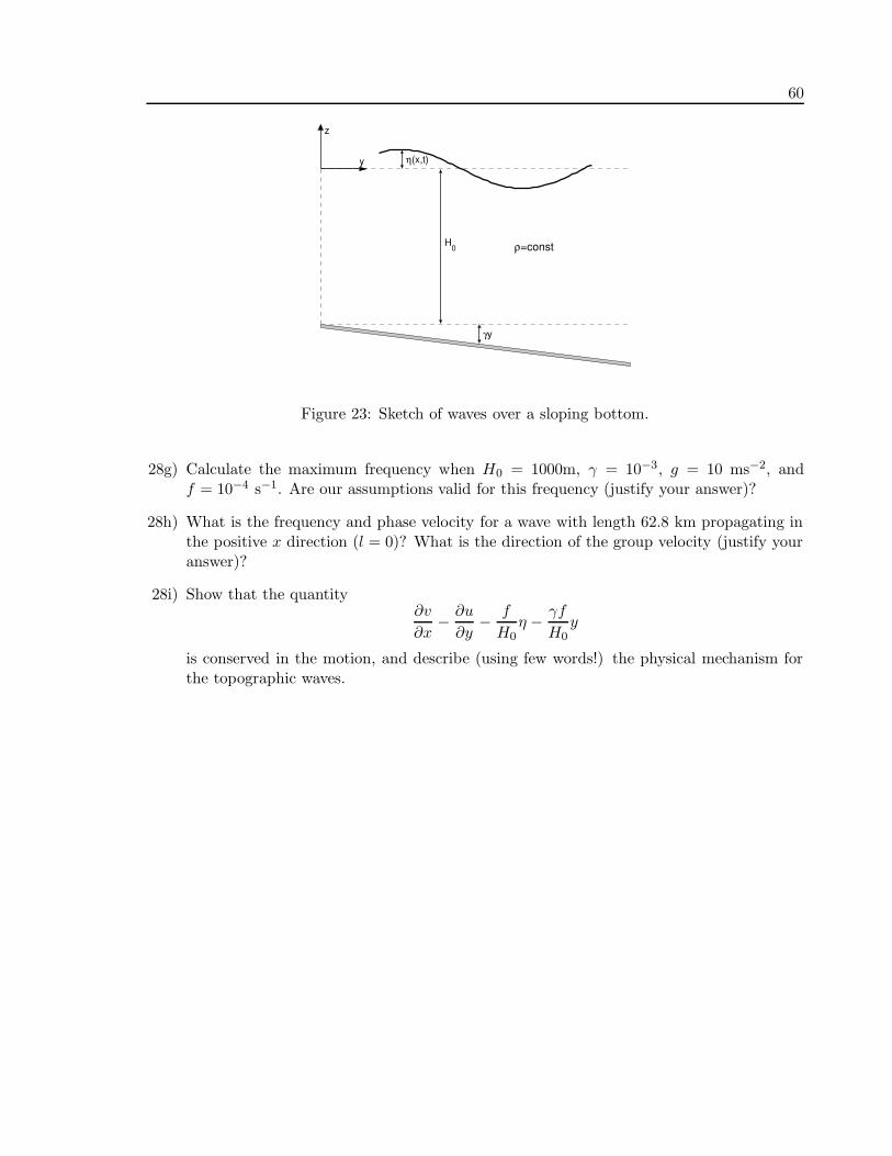
60
z
y η(x,t)
H0
γy
ρ=const
Figure 23: Sketch of waves over a sloping bottom.
28g) Calculate the maximum frequency when H0 = 1000m, γ = 10−3, g = 10 ms−2, andf = 10−4 s−1. Are our assumptions valid for this frequency (justify your answer)?
28h) What is the frequency and phase velocity for a wave with length 62.8 km propagating inthe positive x direction (l = 0)? What is the direction of the group velocity (justify youranswer)?
28i) Show that the quantity∂v
∂x− ∂u
∂y− f
H0η − γf
H0y
is conserved in the motion, and describe (using few words!) the physical mechanism forthe topographic waves.

61
29 Equatorial Kelvin Waves
In this section we will study the strongest natural climate variability signal on the globe, the ElNino in the Pacific. During periods of a weakening or even reversal of the trade winds, eastwardpropagating equatorial Kelvin waves are generated, that eventually causes anomalous highsurface temperatures in the eastern Pacific (see Figure 24). These situations with anomalouslywarm water are known as El Nino episodes, and they have large impacts on weather over largeparts of the globe.
29a) We assume that we can describe the Equatorial region as a two-layer system, wheredensity in the upper layer is ρ1, density in the lower layer is ρ2, and mean thickness ofthe upper layer is H. Disturbances on the surface is denoted by η (positive upward) andthe thickness of the upper layer is given by h. Show that the hydrostatic pressure in thelower layer is given by
p2 = ρ1gh + ρ2g(η − h − z). (1)
29b) Show that if the lower layer is at rest, the relationship between the surface elevation andthe interphase displacement is
η =ρ2 − ρ1
ρ2h. (2)
29c) Near the equator the Coriolis parameter f is to a good approximation given as βy, whereβ = ∂f/∂y ≈ 2.3 × 10⁻¹¹ m−1s−1. Show that the equations that governs the flow in theupper layer can be written
∂u
∂t− βyv = −g′
∂h
∂x(3)
∂v
∂t+ βyu = −g′
∂h
∂y(4)
∂h
∂t+ H(
∂u
∂x+
∂v
∂y) = 0. (5)
29d) Due to the fact that the Coriolis parameter changes sign at the Equator, these equationsadmit a solution that has no flow in the meridional direction, i.e. v = 0. Use thisassumption and derive a wave equation for the amplitude of the interphase h.
29e) We will for wave solutions of the form h = F (y) cos(kx − ωt) + G(y) cos(kx + ωt). Whatis the phase speed of such waves? Are they dispersive?
29f) Derive the u component and then use the relationship between u and ∂h/∂y to show that
dF
dy= −βy
cF and
dG
dy=
βy
cG, (6)
where c = ω/k is the phase speed of the waves.
29g) Integrate the two equation in (6) to show that the solution to our problem becomes
h = h0e−βy2/2c cos(kx − ωt), (7)
u =c
He−βy2/2c cos(kx − ωt), (8)
v = 0. (9)

62
Why did we have to discard the solution travelling towards west?
29h) Typical densities along the Equator is ρ1 = 1023 kgm−3 for the upper layer and ρ2 = 1025kgm−3 for the lower layer, and the mean depth of the upper layer can be set to H = 200m. What is the speed of the signal? Compare your results with what you see in Figure 24.
29i) Assume that we have individual measurements showing that the maximum fluid velocityassociated with the wave is u=0.5 ms−1. What will be the corresponding maximumdisplacement of the interphase? Is your result comparable to what you see in Figure 24?

63
(a)
(b)
Figure 24: Time-distance plot showing (a) the zonal wind speed in the western Pacific (densecurve) and the depth of the 20C isotherm along the Equator, and (b) the sea surface tem-perature along the Equator. The thick lines indicate when there are evidence of eastwardpropagating Kelvin waves, responsible for El Nino episodes. The strongest episode starts in thewinter of 1991-1992, when the trade winds in the western Pacific reversed, and blowed towardseast for several months. The result was Kelvin waves seen as a deepening of the upper layerthat propagated across the Pacific in less than 2 months (≈ 2 ms−1), and the result is seen asvery high surface temperatures in the eastern Pacific during the spring of 1992 (from Kessleret al 1995, Journal of Geophysical Research, 100(C6), 10613–10631).

64
30 Planetary waves
Through a series of publications in the 1930s the Swede C. G. Rossby demonstrated that thereexisted a kind of waves in the world oceans that propagates so slowly that they will use severalyears or even decades to cross the Pacific or the Atlantic Oceans. It was first through analysisof satellite images in the 1990s that one has managed to identify these waves that we now knowas Rossby waves. An example from the North Atlantic is shown in Figure 25.
As such waves has so large horizontal extension, one has to take into account that theCoriolis parameter f varies with the latitude. We therefore write f = f0 + βy where f0 is theconstant value in y = 0 and β ≡ df/dy is a constant. The equations that describe the Rossbywaves can be written12.
∂u
∂t− (f0 + βy)v = −1
ρ
∂p
∂x
∂v
∂t+ (f0 + βy)u = −1
ρ
∂p
∂y
0 = −1
ρ
∂p
∂z− g
∂u
∂x+
∂v
∂y+
∂w
∂z= 0.
30a) We will look at a two-layer model with an active upper layer having density ρ1 and meanthickness H, and a deep lower layer with density ρ2 and no flow (u = v = 0). The surfaceelevation is given by z = η and a perturbation on the interface between the two layers asz = −H + h. Show that the velocities in the upper layer may be written as
∂u
∂t− (f0 + βy)v = g′
∂h
∂x∂v
∂t+ (f0 + βy)u = g′
∂h
∂y
∂h
∂t− H(
∂u
∂x+
∂v
∂y) = 0,
where g′ = (ρ2 − ρ1)g/ρ1 and we apply the approximation that we neglect the surfaceelevation in the equation of continuity. What is the name of this approximation?
30b) As the Rossby waves have time scales that are much larger than the rotation period of theEarth, we can use the quasi-geostrophic approximation. Show that this gives the followingequations for the velocity components u and v:
u = +g′
f0
∂h
∂y+
g′
f20
∂2h
∂x∂t− βg′
f20
y∂h
∂y
v = − g′
f0
∂h
∂x+
g′
f20
∂2h
∂y∂t+
βg′
f20
y∂h
∂x
12This exercise was given at the GEOF330 exam 8. December 2004.

65
30c) Show that the wave equation becomes
∂h
∂t− a2(
∂2
∂x2+
∂2
∂y2)∂h
∂t− βa2 ∂h
∂x= 0, where a2 =
g′H
f20
.
30d) Assume a wave component on the form h = h0 cos(kx + ly − ωt) (or use complex form ifyou wish), and show that the dispersion relation for the baroclinic Rossby wave is givenas
ω = − βa2k
1 + a2(k2 + l2).
Let the north-south component l = 0, and and discuss the phase- and group velocities forvery short and very long waves.
30e) Use the quasi-geostrophic assumptions for u and v to show that the ratio between thekinetic and the potential energy per wave length is given as
kinetic energy density
potential energy density= (k2 + l2)a2.
Discuss the solution for short and long wave lengths.
30f) From Figure 25b we read typical wave length and wave period for the waves travellingalong 34N to be 600 km and 6 months respectively. Calculate the Rossby radius a, thephase velocity cp and the group velocity cg. Where do you think the waves are generated?
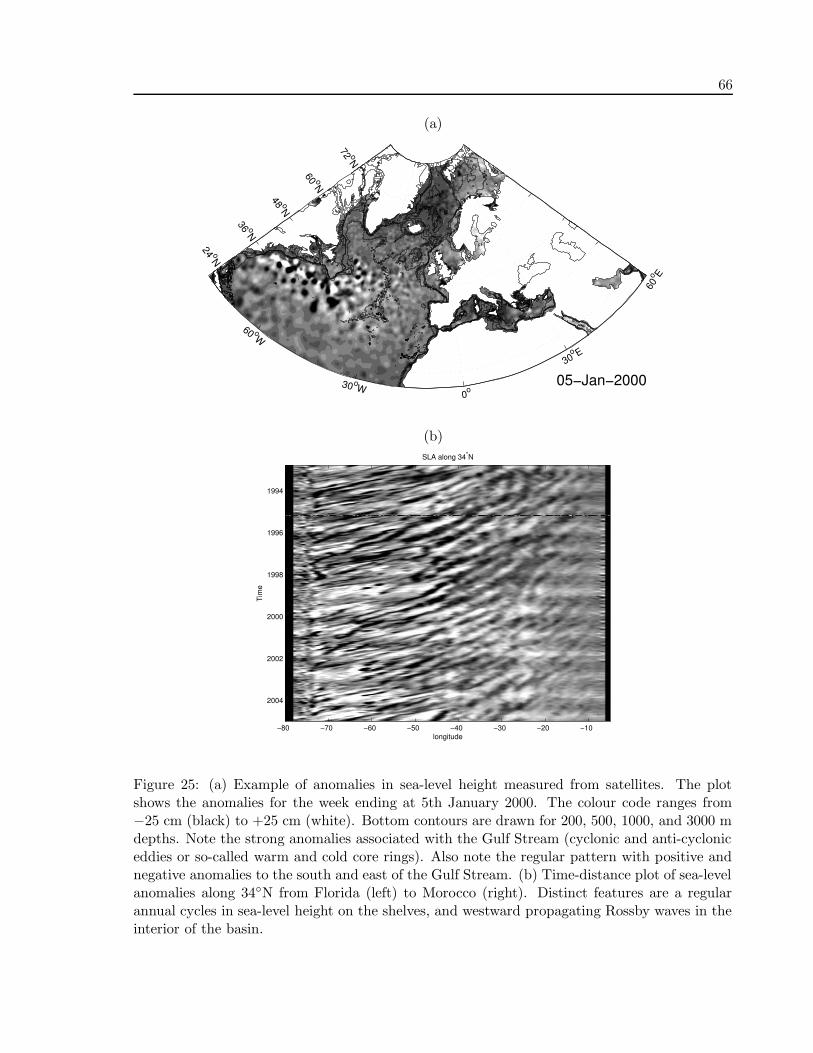
66
(a)
60 oW
30 oW 0o
30o E
60
o E
24 oN
36 oN 48 oN
60 oN 72 oN
05−Jan−2000
(b)
longitude
Tim
e
SLA along 34°N
−80 −70 −60 −50 −40 −30 −20 −10
1994
1996
1998
2000
2002
2004
Figure 25: (a) Example of anomalies in sea-level height measured from satellites. The plotshows the anomalies for the week ending at 5th January 2000. The colour code ranges from−25 cm (black) to +25 cm (white). Bottom contours are drawn for 200, 500, 1000, and 3000 mdepths. Note the strong anomalies associated with the Gulf Stream (cyclonic and anti-cycloniceddies or so-called warm and cold core rings). Also note the regular pattern with positive andnegative anomalies to the south and east of the Gulf Stream. (b) Time-distance plot of sea-levelanomalies along 34N from Florida (left) to Morocco (right). Distinct features are a regularannual cycles in sea-level height on the shelves, and westward propagating Rossby waves in theinterior of the basin.