ATM 111

Weather Map Discussion

R. Grotjahn

W 2005

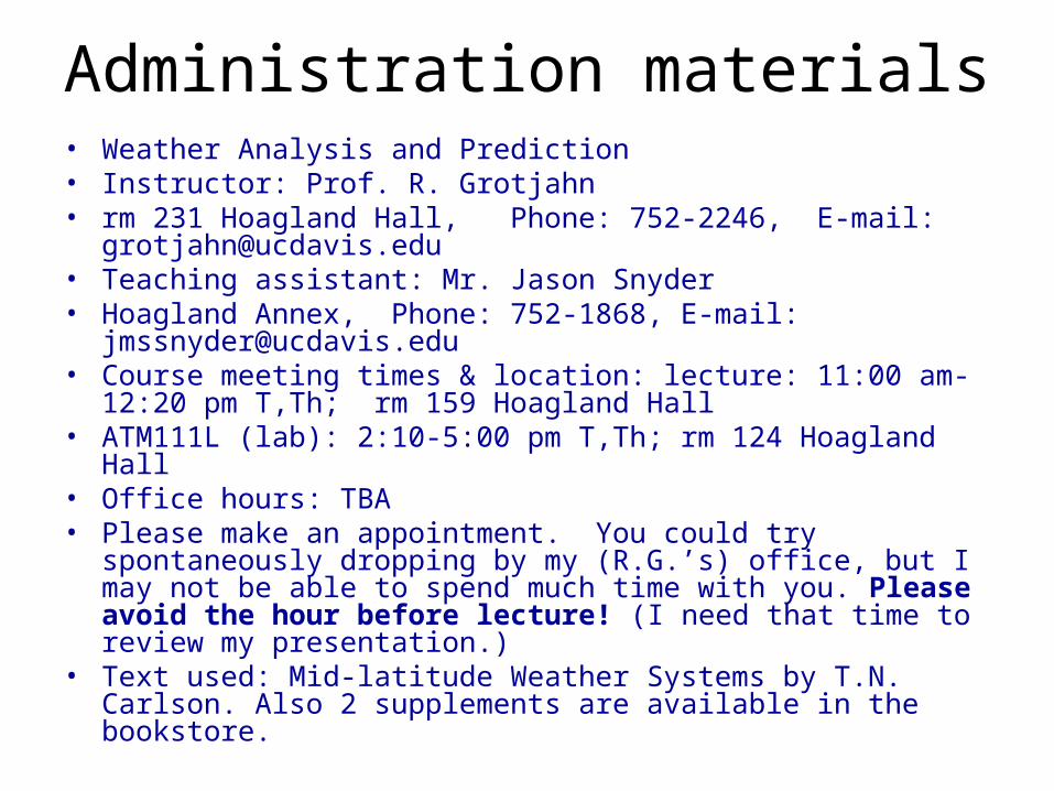
Administration materials• Weather Analysis and Prediction• Instructor: Prof. R. Grotjahn• rm 231 Hoagland Hall, Phone: 752-2246, E-mail:

grotjahn@ucdavis.edu• Teaching assistant: Mr. Jason Snyder• Hoagland Annex, Phone: 752-1868, E-mail:

jmssnyder@ucdavis.edu• Course meeting times & location: lecture: 11:00 am-12:20 pm T,Th;

rm 159 Hoagland Hall• ATM111L (lab): 2:10-5:00 pm T,Th; rm 124 Hoagland Hall• Office hours: TBA• Please make an appointment. You could try spontaneously

dropping by my (R.G.’s) office, but I may not be able to spend much time with you. Please avoid the hour before lecture! (I need that time to review my presentation.)

• Text used: Mid-latitude Weather Systems by T.N. Carlson. Also 2 supplements are available in the bookstore.

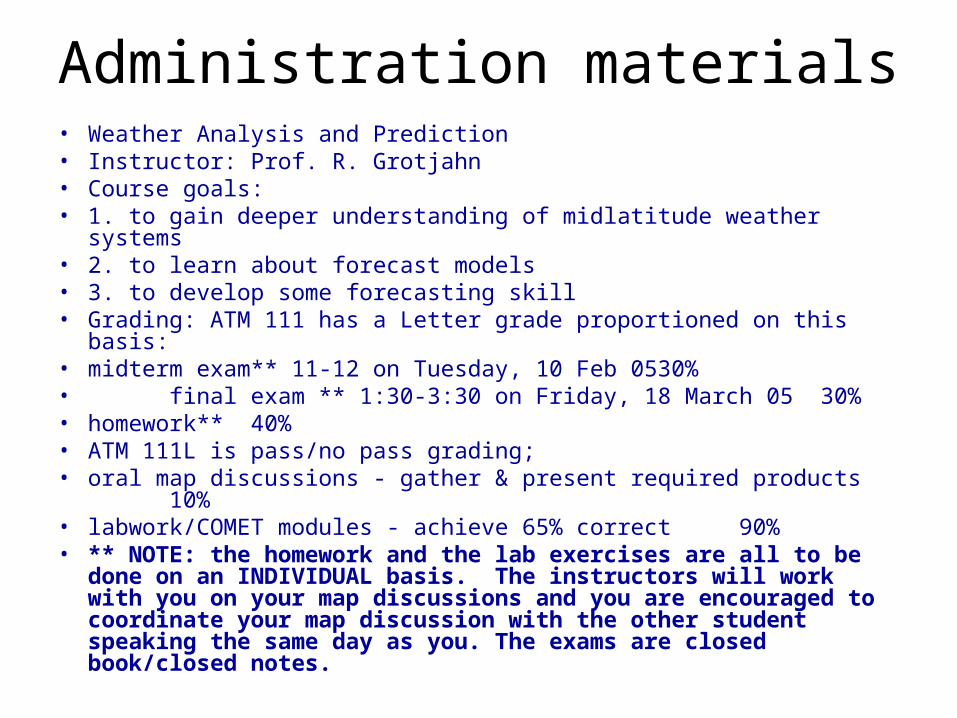
Administration materials• Weather Analysis and Prediction• Instructor: Prof. R. Grotjahn• Course goals:• 1. to gain deeper understanding of midlatitude weather systems• 2. to learn about forecast models• 3. to develop some forecasting skill• Grading: ATM 111 has a Letter grade proportioned on this basis: • midterm exam** 11-12 on Tuesday, 10 Feb 05 30%• final exam ** 1:30-3:30 on Friday, 18 March 05 30%• homework** 40%• ATM 111L is pass/no pass grading; • oral map discussions - gather & present required products 10%• labwork/COMET modules - achieve 65% correct 90%• ** NOTE: the homework and the lab exercises are all to be done

on an INDIVIDUAL basis. The instructors will work with you on your map discussions and you are encouraged to coordinate your map discussion with the other student speaking the same day as you. The exams are closed book/closed notes.

Forecast Notebook

• information presented there addresses same four questions each time: – (1) Why look at this chart, image or map?– (2) What features on this product should

be noted?– (3) What aspects of those features are

significant?– (4) What do those aspects of those

features signify?

Oral Presentations General Advice

• Follow format in the forecast notebook• Avoid common pitfalls:

– Familiarize yourself with the equipment before your presentation – images load quicker off of the hard drive – Use short, descriptive file names in your own directory for each

file. – The machine is slowed down if many applications are running – Only a portion of the object may be displayed on the projection

screen – not leaving enough time to think about what you are going to

say – Try not to show too many maps

Map Review of Recent Weathera. Primary charts:• hemispheric and N. American 500 mb Z

– i. overview of major troughs, ridges, short-waves. present location & motion– ii. (geostrophic) wind pattern (jet axis, direction of flow, etc.)– iii. possible PVA, NVA locations

• 1000/500 mb thickness (N. America or hemis. if N. Am. not available)– i. for assessing warm & cold air masses, – ii. finding occluded fronts– iii. possible locations of WAA, CAA

• 500mb Z overlay on IR satellite -- link Z pattern & satellite imagery• satellite imagery (N. Pacific, N. America) latest image AND loops

– i. see motion of main systems– ii. usually use IR, especially for loops.– iii. visible imagery useful for finding fog and other special events

• current radar imagery – i. see which clouds are precipitating and what type of precip

• current surface chart -- try to explain: – i. all areas of precip, – ii. identify locations of major fronts & trofs and their properties (e.g. type,

intensity, change, direction of motion). – iii. other unusual weather like severe winds, severe convection, fog, hard freezes,

etc.

Map Review of Recent Weatherb. Supplementary charts (as needed to justify explanations

& information presented above)• 200/300 mb level Z and isotachs –

– jet stream, especially jet streaks location(s)

• skew-T ln-P charts -- useful for discussion of: – i. convection, – ii. freezing rain, – iii. cloud depths, etc.– iv. alternatives: LI, 4 panel moisture, or CAPE charts

• meteograms -- useful for noting a time sequence at a station:– i. frontal passage– ii. time of occurrence of max T or min T, or precip.

• potential temperature charts -- assessing potential vorticity (PV) movement

Review of Recent Model Performance2. a. Review recent forecasts (e.g. compare models’ 12 or

24 hr fcsts with most recent obs). Maybe human forecasters and MOS.

• 500 mb Z – i. compare troughs (locations, strengths, orientation & shape)– ii. location of strongest gradient (e.g. geostrophic wind jet)

• surface chart – i. compare SLP (locations, strengths, and shapes of highs and

lows)– ii. areas of precipitation

• 24 hour precip chart -- how does distribution & amount of precip compare to fcst in past 24 hrs?

• b. Specific forecasts: 24 hour max T & min T -- how did

guidance and forecasters do?

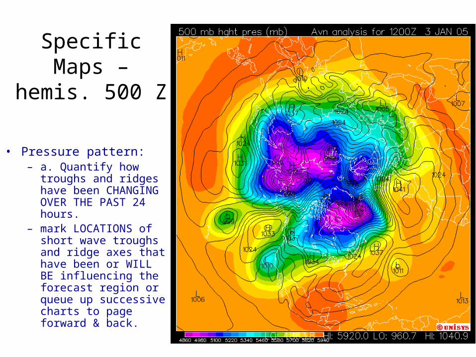
Specific Maps – hemis. 500 Z

• Pressure pattern:– a. Quantify how

troughs and ridges have been CHANGING OVER THE PAST 24 hours.

– mark LOCATIONS of short wave troughs and ridge axes that have been or WILL BE influencing the forecast region or queue up successive charts to page forward & back.

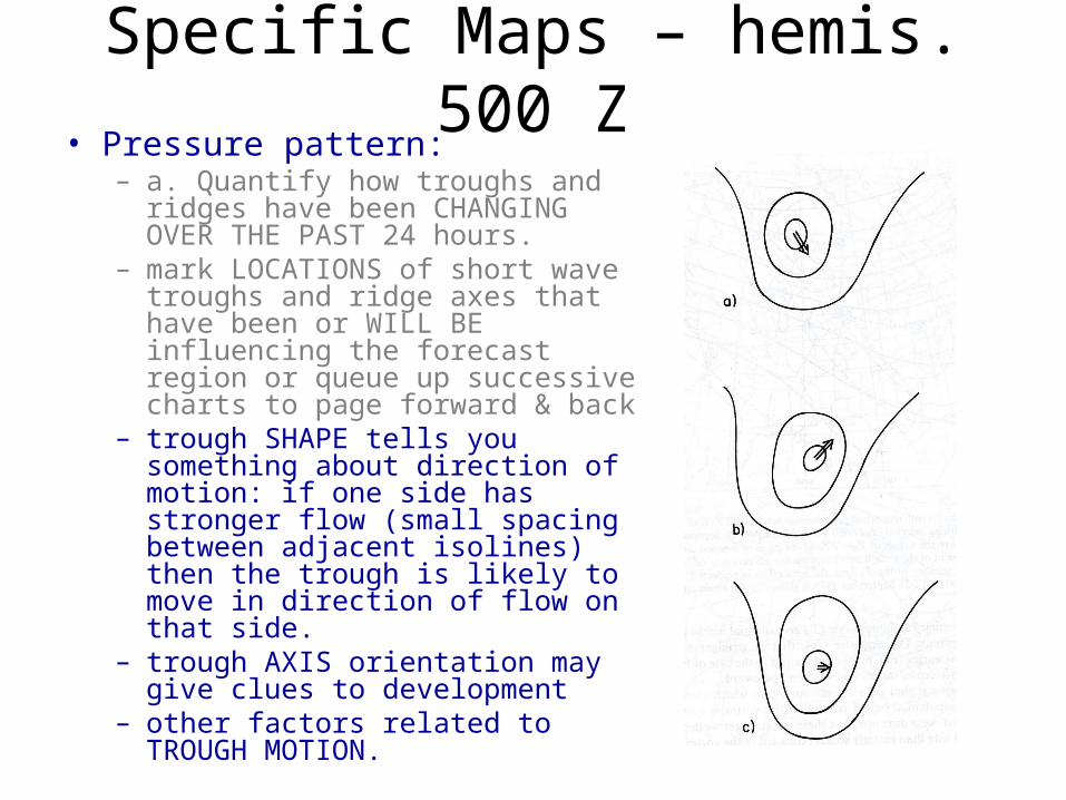
Specific Maps – hemis. 500 Z• Pressure pattern:

– a. Quantify how troughs and ridges have been CHANGING OVER THE PAST 24 hours.

– mark LOCATIONS of short wave troughs and ridge axes that have been or WILL BE influencing the forecast region or queue up successive charts to page forward & back

– trough SHAPE tells you something about direction of motion: if one side has stronger flow (small spacing between adjacent isolines) then the trough is likely to move in direction of flow on that side.

– trough AXIS orientation may give clues to development

– other factors related to TROUGH MOTION.

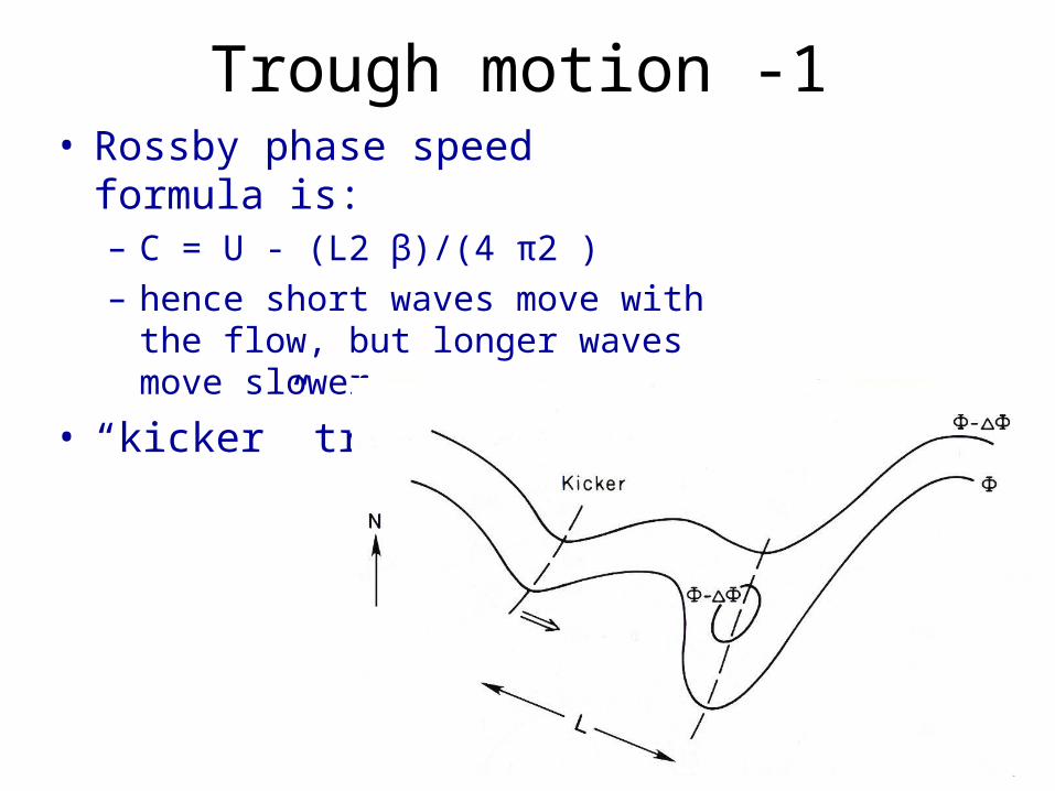
Trough motion -1• Rossby phase speed formula is:

– C = U - (L2 β)/(4 π2 )– hence short waves move with the

flow, but longer waves move slower.

• “kicker” trough.

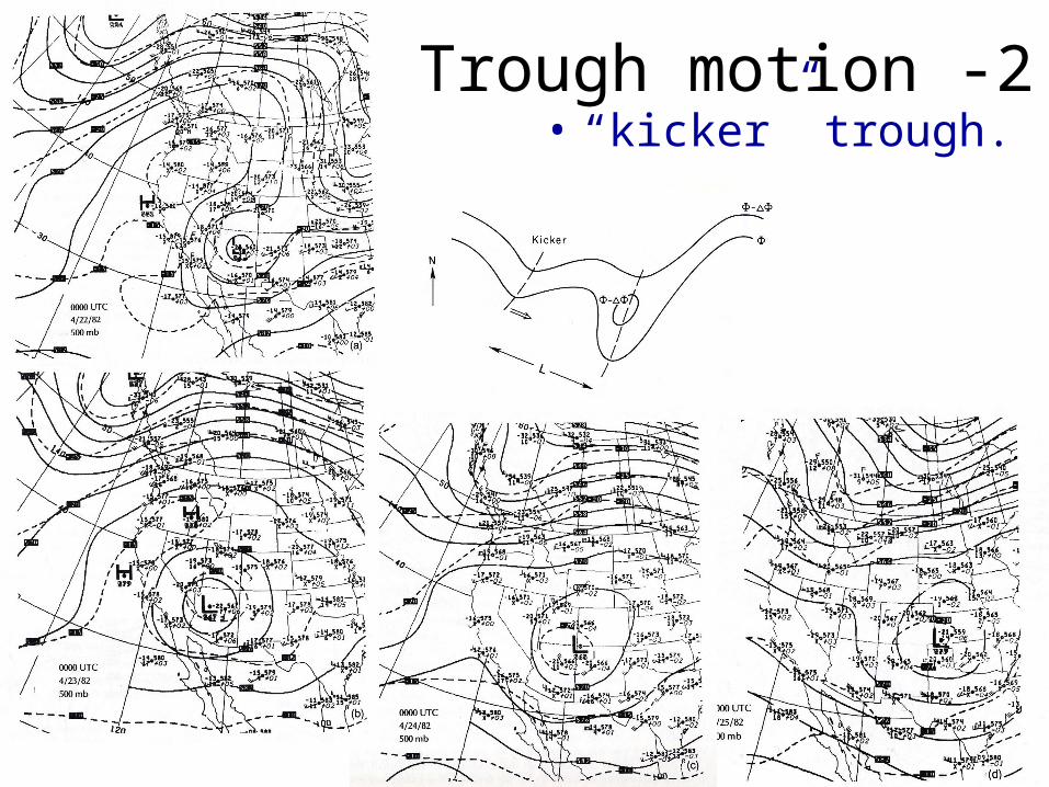
Trough motion -2• “kicker” trough.

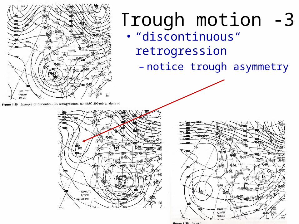
Trough motion -3• “discontinuous

retrogression” – notice trough asymmetry

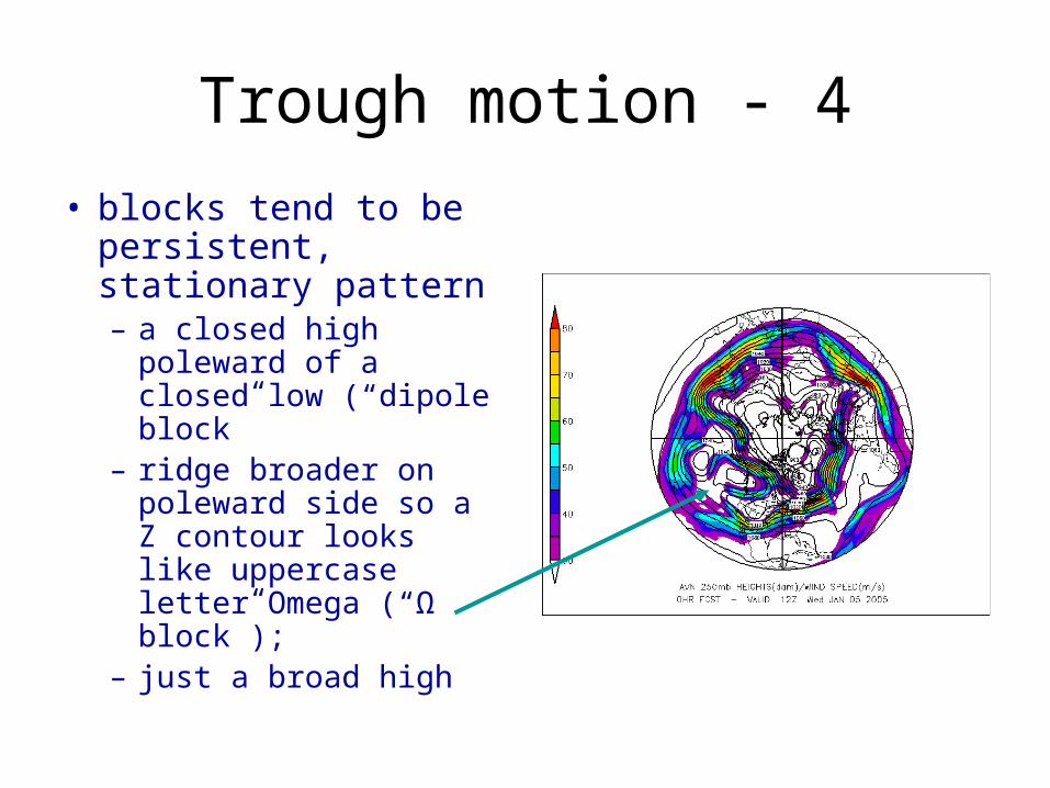
Trough motion - 4

• blocks tend to be persistent, stationary pattern– a closed high poleward

of a closed low (“dipole block”

– ridge broader on poleward side so a Z contour looks like uppercase letter Omega (“Ω block”);

– just a broad high

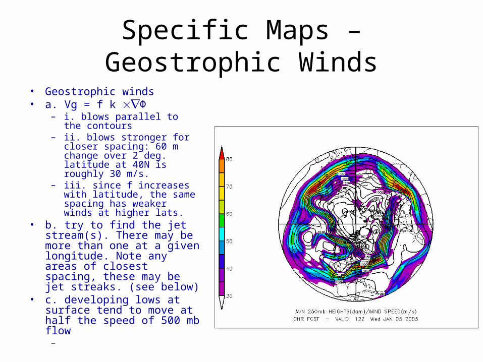
Specific Maps – Geostrophic Winds

• Geostrophic winds• a. Vg = f k Φ

– i. blows parallel to the contours

– ii. blows stronger for closer spacing: 60 m change over 2 deg. latitude at 40N is roughly 30 m/s.

– iii. since f increases with latitude, the same spacing has weaker winds at higher lats.

• b. try to find the jet stream(s). There may be more than one at a given longitude. Note any areas of closest spacing, these may be jet streaks. (see below)

• c. developing lows at surface tend to move at half the speed of 500 mb flow

–

Specific Maps – N. America 500 Z• PVA & NVA from geostrophic

wind and vorticity: – i. PVA and NVA occur as a

“dipole” pair; one ahead and one behind vorticity extremum. PVA behind a ridge; NVA behind a trough.

– ii. From the omega equation: PVA encourages upward motion, NVA encourages downward motion. Such motion is not guaranteed: other factors may compensate, such as temperature advection.

– iii. If NVA causes downward motion, then that implies such possibilities as: clearing & bringing strong winds down to the surface.

– iv. If PVA causes upward motion, then that may imply: cloudiness, precipitation

Specific Maps –Thickness -1• a. Thickness is

proportional to mean T in a layer so, assess warm & cold air masses, – i. identify areas

of warmer and colder air masses

– ii. identify how intense such air masses are (by low values of thickness)

colors: SLP black: 1000-500 hPa thickness

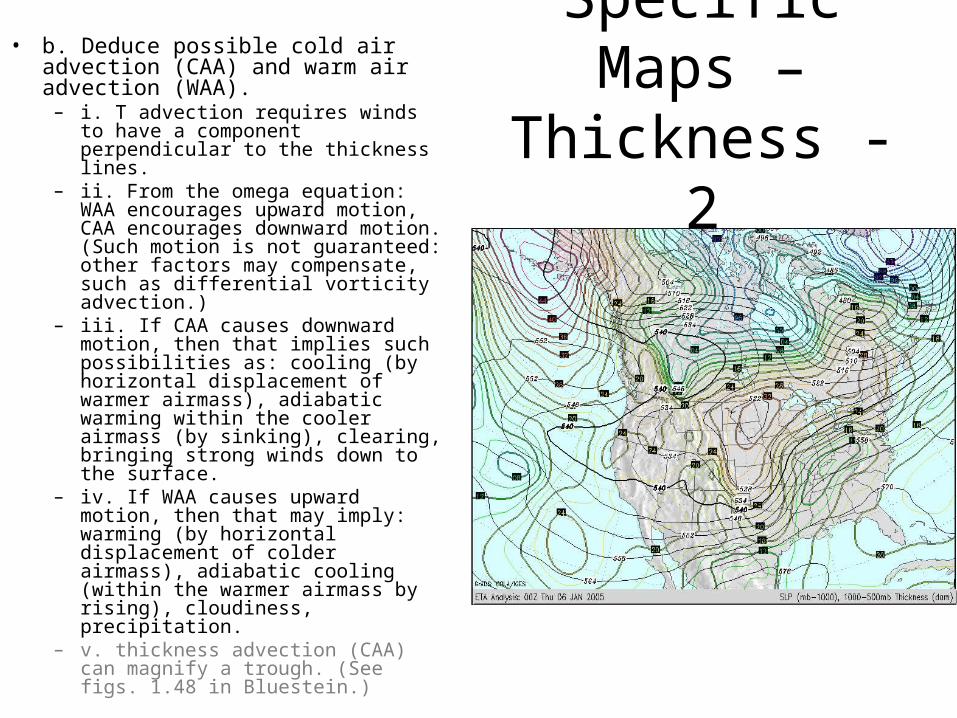
Specific Maps –Thickness - 2

• b. Deduce possible cold air advection (CAA) and warm air advection (WAA).

– i. T advection requires winds to have a component perpendicular to the thickness lines.

– ii. From the omega equation: WAA encourages upward motion, CAA encourages downward motion. (Such motion is not guaranteed: other factors may compensate, such as differential vorticity advection.)

– iii. If CAA causes downward motion, then that implies such possibilities as: cooling (by horizontal displacement of warmer airmass), adiabatic warming within the cooler airmass (by sinking), clearing, bringing strong winds down to the surface.

– iv. If WAA causes upward motion, then that may imply: warming (by horizontal displacement of colder airmass), adiabatic cooling (within the warmer airmass by rising), cloudiness, precipitation.

– v. thickness advection (CAA) can magnify a trough. (See figs. 1.48 in Bluestein.)

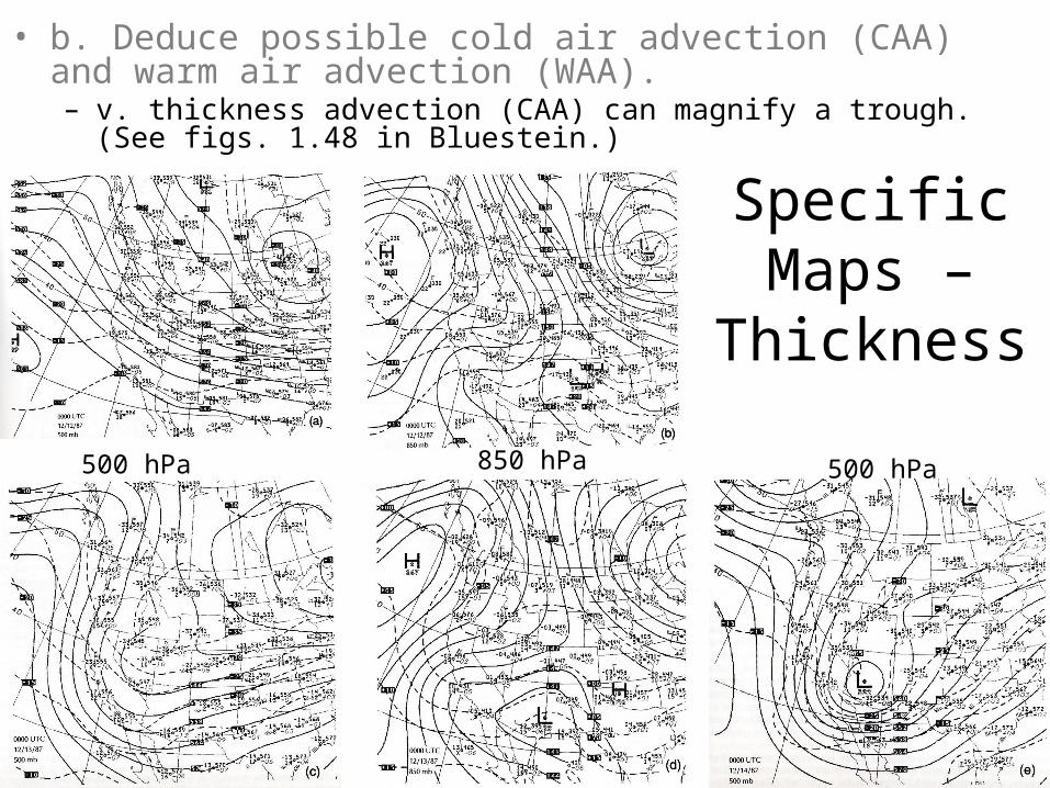
Specific Maps –

Thickness

• b. Deduce possible cold air advection (CAA) and warm air advection (WAA).– v. thickness advection (CAA) can magnify a trough. (See figs. 1.48 in

Bluestein.)

500 hPa 850 hPa 500 hPa

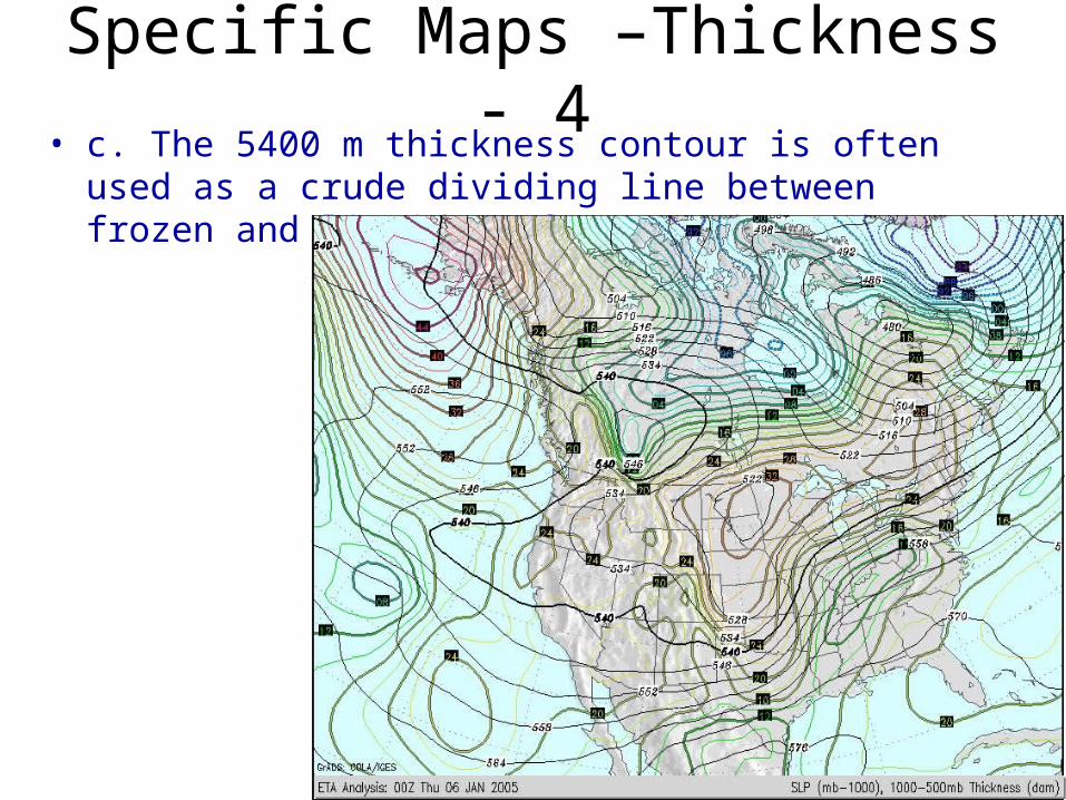
Specific Maps –Thickness - 4• c. The 5400 m thickness contour is often used as a crude

dividing line between frozen and liquid surface precipitation.

Specific Maps –Thickness - 5

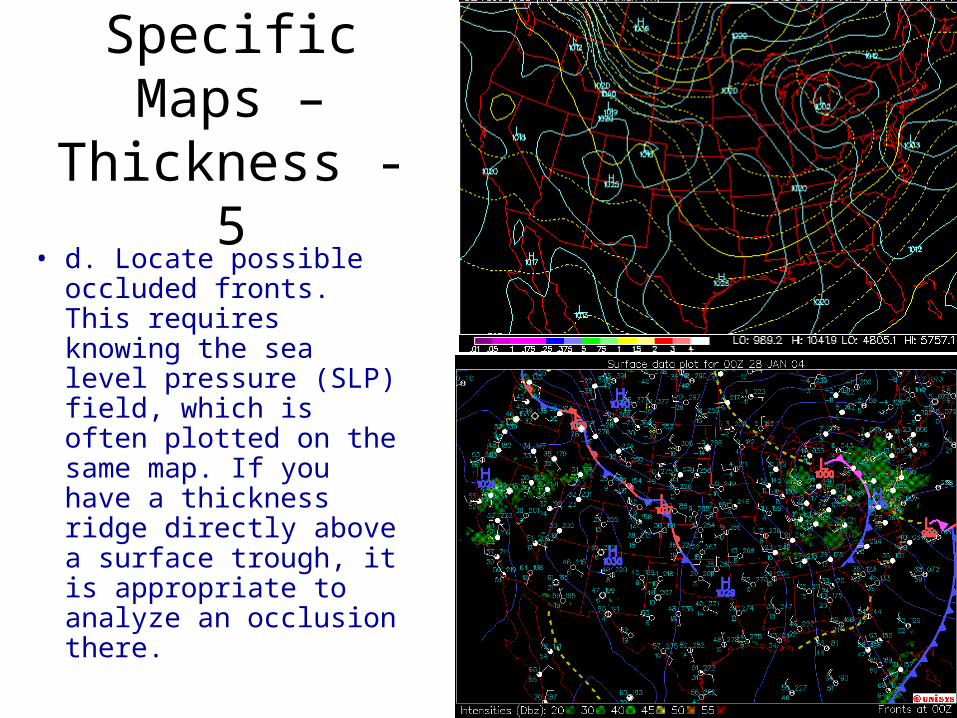
• d. Locate possible occluded fronts. This requires knowing the sea level pressure (SLP) field, which is often plotted on the same map. If you have a thickness ridge directly above a surface trough, it is appropriate to analyze an occlusion there.

Specific Maps – Satellite & 500 Z

overlay

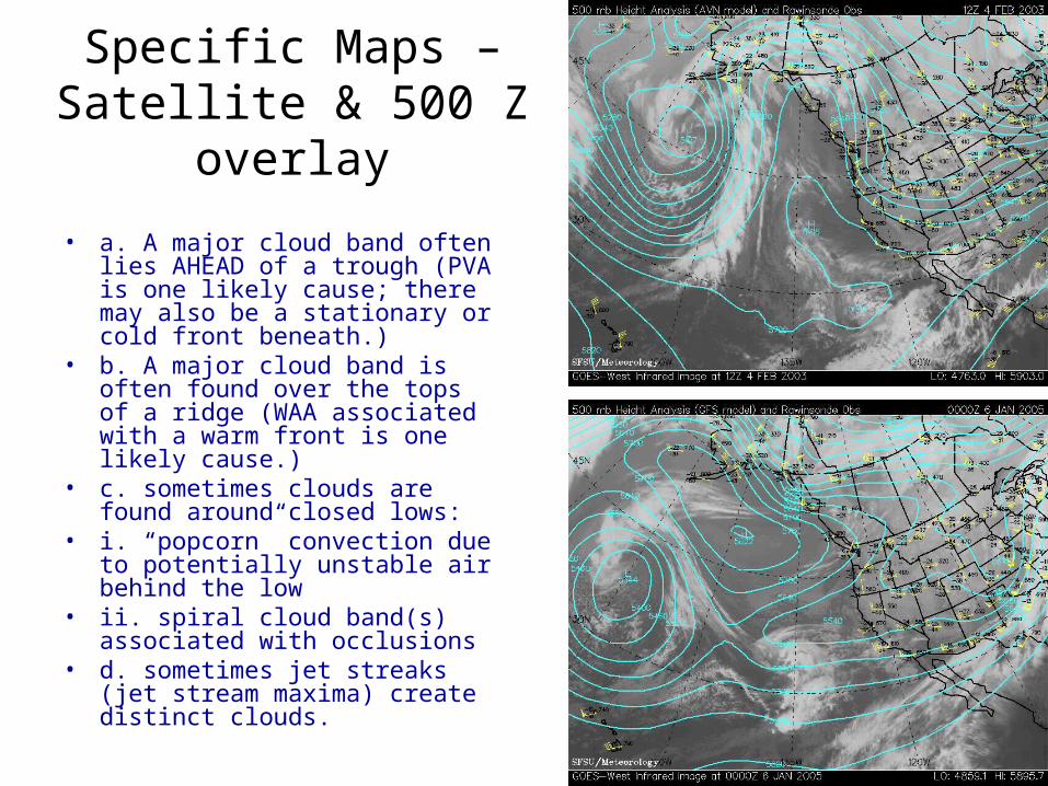
• a. A major cloud band often lies AHEAD of a trough (PVA is one likely cause; there may also be a stationary or cold front beneath.)

• b. A major cloud band is often found over the tops of a ridge (WAA associated with a warm front is one likely cause.)

• c. sometimes clouds are found around closed lows:

• i. “popcorn” convection due to potentially unstable air behind the low

• ii. spiral cloud band(s) associated with occlusions

• d. sometimes jet streaks (jet stream maxima) create distinct clouds.

Specific Maps – Satellite loops

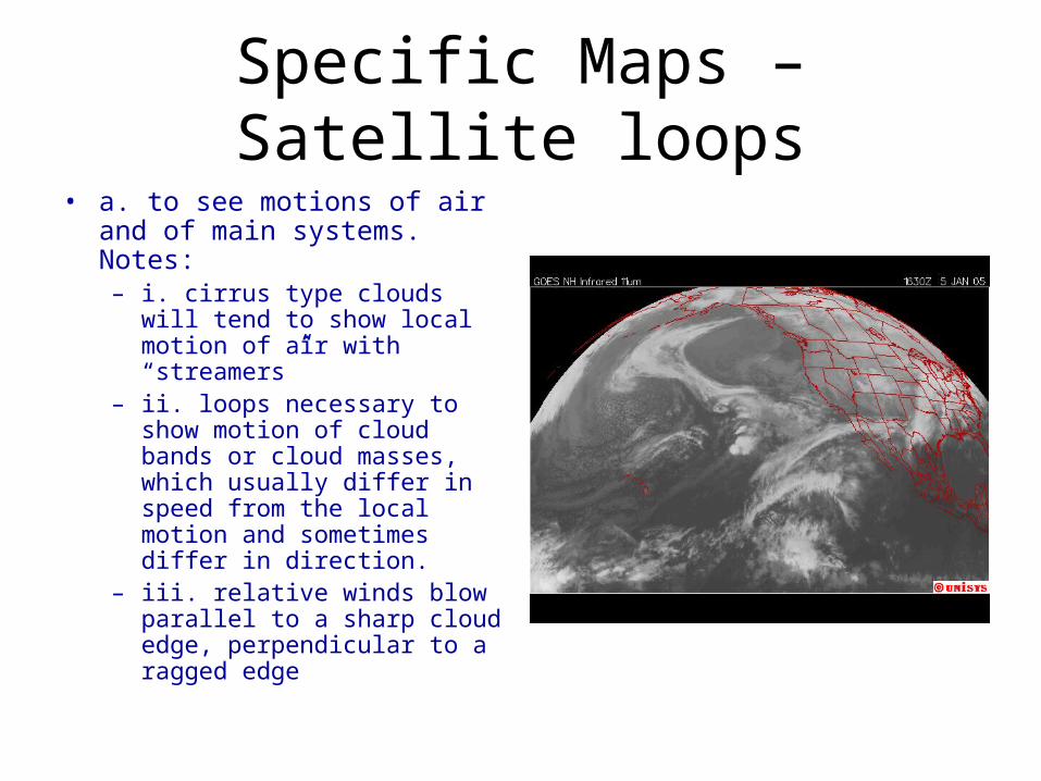
• a. to see motions of air and of main systems. Notes: – i. cirrus type clouds will tend to

show local motion of air with “streamers”

– ii. loops necessary to show motion of cloud bands or cloud masses, which usually differ in speed from the local motion and sometimes differ in direction.

– iii. relative winds blow parallel to a sharp cloud edge, perpendicular to a ragged edge

Specific Maps – Satellite imagery

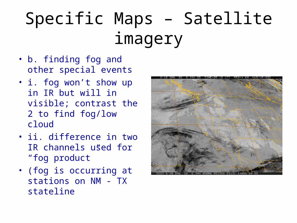
• b. finding fog and other special events

• i. fog won’t show up in IR but will in visible; contrast the 2 to find fog/low cloud

• ii. difference in two IR channels used for “fog product”

• (fog is occurring at stations on NM - TX stateline

Specific Maps – Satellite imagery• c. special uses:• i. jet streams and jet streaks: • 1. cloud often on anticyclone shear side of subtropical jet stream (e.g. Baja)• 2. on the left rear quadrant of jet streak the cloud has a sharp edge in IR,

visible or vapor channel images. A water vapor channel image of a generally cloudy area where the jet lies, may have a region with a sharp boundary between dry and moist air, the jet streak is centered at the leading portion of this sharp edge. (See p. 366-68 and p. 409, in Carlson book) (Bader et al: p. 204, 100, etc.)

Specific Maps – Satellite imagery

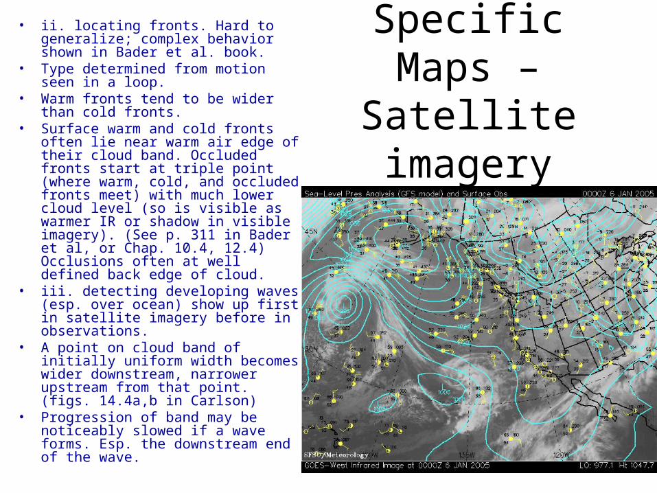
• ii. locating fronts. Hard to generalize; complex behavior shown in Bader et al. book.

• Type determined from motion seen in a loop.

• Warm fronts tend to be wider than cold fronts.

• Surface warm and cold fronts often lie near warm air edge of their cloud band. Occluded fronts start at triple point (where warm, cold, and occluded fronts meet) with much lower cloud level (so is visible as warmer IR or shadow in visible imagery). (See p. 311 in Bader et al, or Chap. 10.4, 12.4) Occlusions often at well defined back edge of cloud.

• iii. detecting developing waves (esp. over ocean) show up first in satellite imagery before in observations.

• A point on cloud band of initially uniform width becomes wider downstream, narrower upstream from that point. (figs. 14.4a,b in Carlson)

• Progression of band may be noticeably slowed if a wave forms. Esp. the downstream end of the wave.

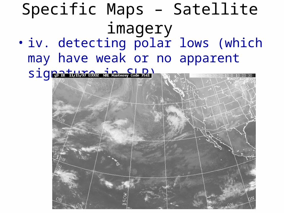
Specific Maps – Satellite imagery

• iv. detecting polar lows (which may have weak or no apparent signature in SLP).

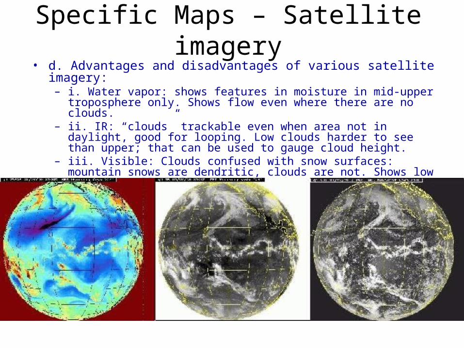
Specific Maps – Satellite imagery• d. Advantages and disadvantages of various satellite imagery:

– i. Water vapor: shows features in moisture in mid-upper troposphere only. Shows flow even where there are no clouds.

– ii. IR: “clouds” trackable even when area not in daylight, good for looping. Low clouds harder to see than upper; that can be used to gauge cloud height.

– iii. Visible: Clouds confused with snow surfaces: mountain snows are dendritic, clouds are not. Shows low clouds equally well as high clouds. Poor for looping.

Specific Maps - Radar

• a.. Relate the larger areas of precip to what already shown..

– i. precip may occur where there is WAA or PVA, especially if both together

– ii. precip may occur if there is moist flow up a mountain slope

– iii. compare with satellite imagery to see which clouds are precipitating and what type of precip

• b. note other information if available:– i. general values of echo tops -- note

extreme heights such as > 45 k ft. Deeper clouds may produce more precip. Snow can fall from very shallow clouds.

– ii. general values of echo bases -- low ceilings important for aviation

– iii. general direction of cell movement vs movement of system as a whole. For convective systems, individual cells that move to the right of the general pattern may be more intense.

– iv. watch for virga may show up -- need to compare overlapping radar scans. v. severe weather watch boxes

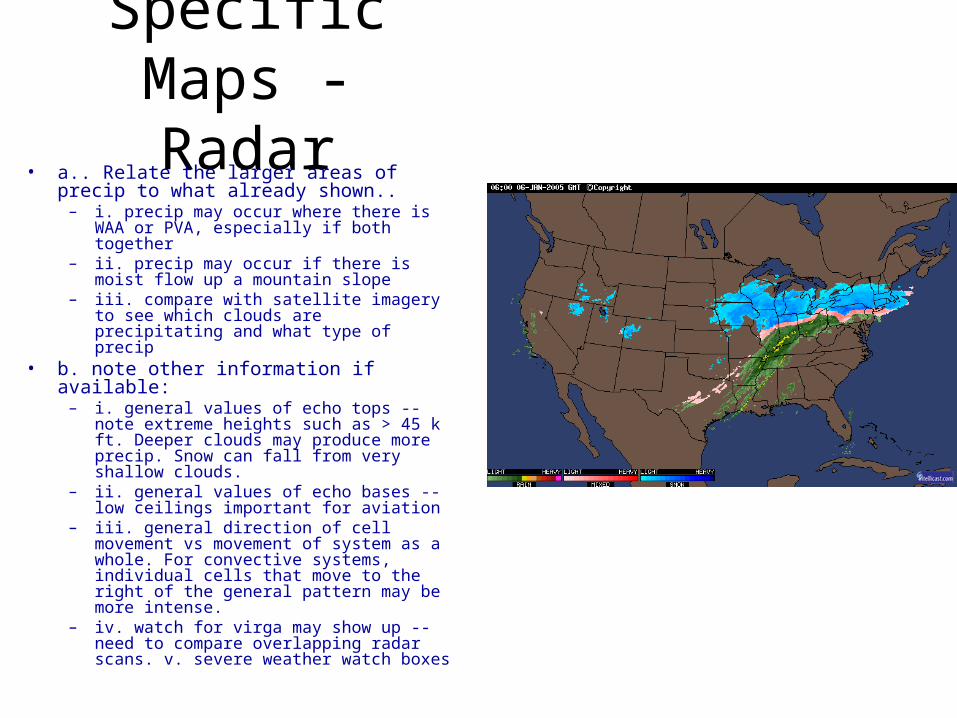
Specific Maps - Radar

• a.. Relate the larger areas of precip to what already shown..

– i. precip may occur where there is WAA or PVA, especially if both together

– ii. precip may occur if there is moist flow up a mountain slope

– iii. compare with satellite imagery to see which clouds are precipitating and what type of precip

• b. note other information if available:– i. general values of echo tops -- note

extreme heights such as > 45 k ft. Deeper clouds may produce more precip. Snow can fall from very shallow clouds.

– ii. general values of echo bases -- low ceilings important for aviation

– iii. general direction of cell movement vs movement of system as a whole. For convective systems, individual cells that move to the right of the general pattern may be more intense.

– iv. watch for virga may show up -- need to compare overlapping radar scans. v. severe weather watch boxes

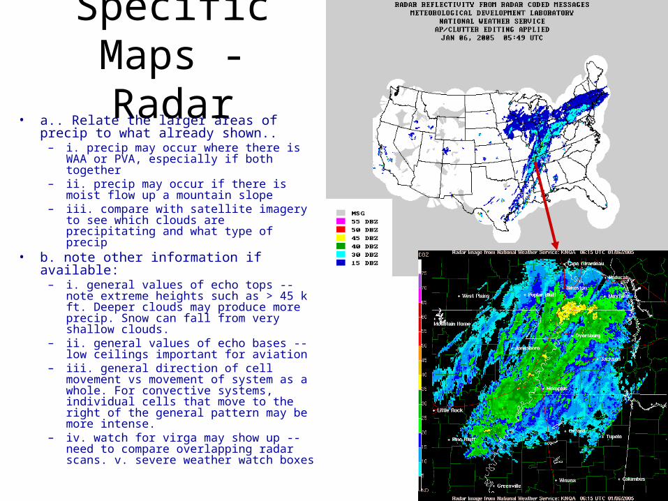
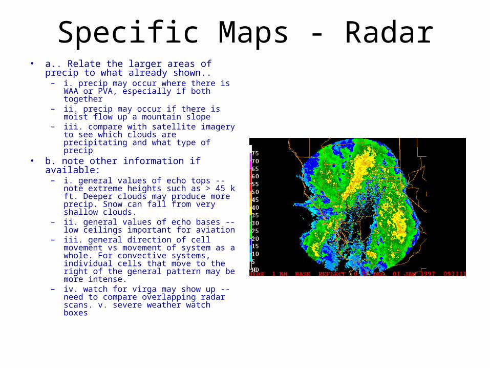
Specific Maps - Radar• a.. Relate the larger areas of precip to

what already shown..– i. precip may occur where there is

WAA or PVA, especially if both together

– ii. precip may occur if there is moist flow up a mountain slope

– iii. compare with satellite imagery to see which clouds are precipitating and what type of precip

• b. note other information if available:– i. general values of echo tops -- note

extreme heights such as > 45 k ft. Deeper clouds may produce more precip. Snow can fall from very shallow clouds.

– ii. general values of echo bases -- low ceilings important for aviation

– iii. general direction of cell movement vs movement of system as a whole. For convective systems, individual cells that move to the right of the general pattern may be more intense.

– iv. watch for virga may show up -- need to compare overlapping radar scans. v. severe weather watch boxes

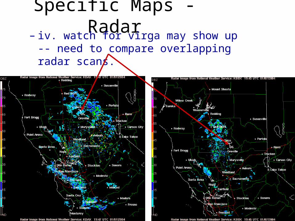
Specific Maps - Radar– iv. watch for virga may show up -- need

to compare overlapping radar scans.

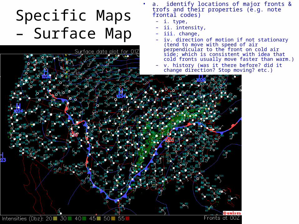
Specific Maps – Surface Map

• a. identify locations of major fronts & trofs and their properties (e.g. note frontal codes)

– i. type, – ii. intensity, – iii. change, – iv. direction of motion if not stationary (tend to

move with speed of air perpendicular to the front on cold air side; which is consistent with idea that cold fronts usually move faster than warm.)

– v. history (was it there before? did it change direction? Stop moving? etc.)

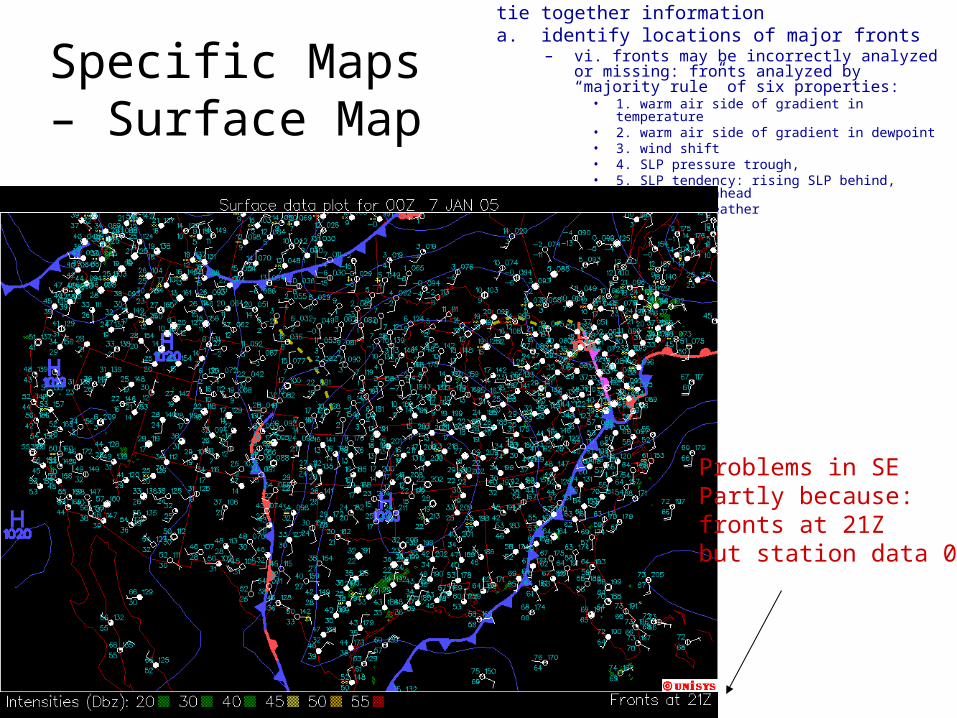
Specific Maps – Surface Map

tie together information a. identify locations of major fronts

– vi. fronts may be incorrectly analyzed or missing: fronts analyzed by “majority rule” of six properties:

• 1. warm air side of gradient in temperature• 2. warm air side of gradient in dewpoint• 3. wind shift• 4. SLP pressure trough, • 5. SLP tendency: rising SLP behind, falling SLP ahead• 6. type of weather

Problems in SEPartly because:fronts at 21Zbut station data 00Z

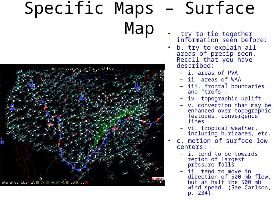
Specific Maps – Surface Map• try to tie together information

seen before:• b. try to explain all areas of

precip seen. Recall that you have described:

– i. areas of PVA– ii. areas of WAA– iii. frontal boundaries and

“trofs”.– iv. topographic uplift – v. convection that may be

enhanced over topographic features, convergence lines

– vi. tropical weather, including huricanes, etc.

• c. motion of surface low centers:

– i. tend to be towards region of largest pressure falls

– ii. tend to move in direction of 500 mb flow, but at half the 500 mb wind speed. (See Carlson, p. 234)

Specific Maps – Surface Map• try to tie together information seen before:• d. watch for significant mesoscale weather (details in later sections)

– i. severe winds, (e.g. Chinooks, Santa Anas, CA central valley northwinds)

– ii. severe convection, squall lines, the Midwest’s “dry line”– iii. sea breezes, – iv. convergence zones– v. fog, (it may not have been noted on the satellite imagery shown)– vi. lake-effect snows (esp. Great Lakes)– vii. freezing rain, sleet

• e. other unusual weather like – i. unusually warm or unusually cold temperatures – ii. dust storms, haze, etc.

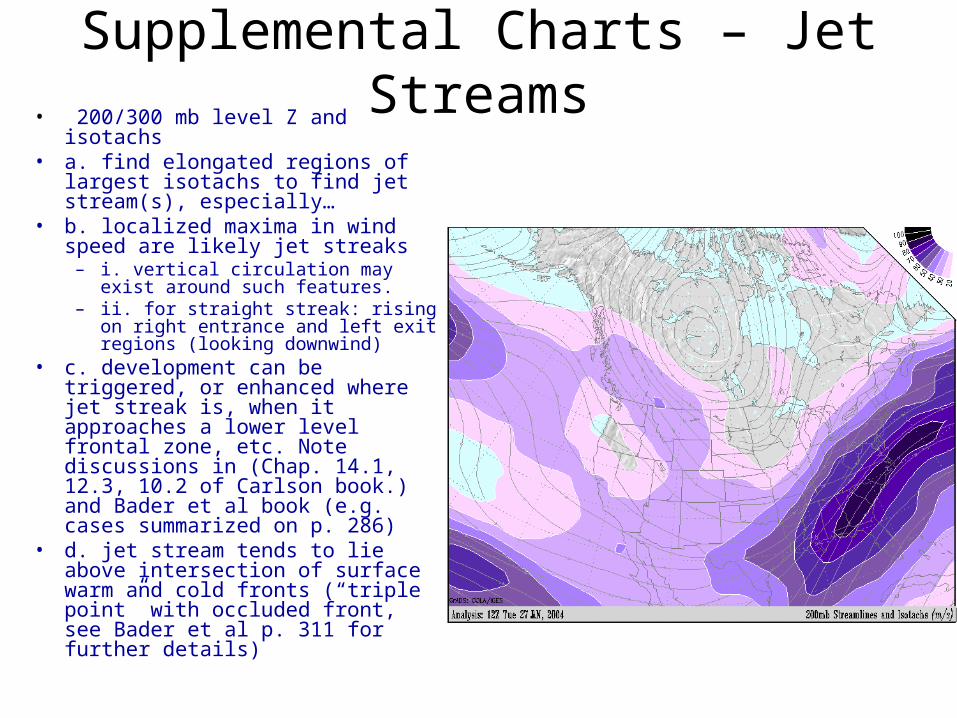
Supplemental Charts – Jet Streams• 200/300 mb level Z and isotachs • a. find elongated regions of largest

isotachs to find jet stream(s), especially…

• b. localized maxima in wind speed are likely jet streaks

– i. vertical circulation may exist around such features.

– ii. for straight streak: rising on right entrance and left exit regions (looking downwind)

• c. development can be triggered, or enhanced where jet streak is, when it approaches a lower level frontal zone, etc. Note discussions in (Chap. 14.1, 12.3, 10.2 of Carlson book.) and Bader et al book (e.g. cases summarized on p. 286)

• d. jet stream tends to lie above intersection of surface warm and cold fronts (“triple point” with occluded front, see Bader et al p. 311 for further details)

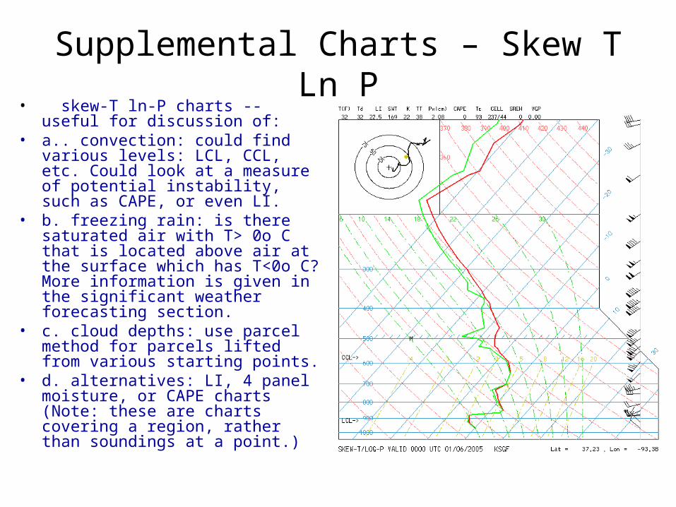
Supplemental Charts – Skew T Ln P• skew-T ln-P charts -- useful for

discussion of: • a.. convection: could find various

levels: LCL, CCL, etc. Could look at a measure of potential instability, such as CAPE, or even LI.

• b. freezing rain: is there saturated air with T> 0o C that is located above air at the surface which has T<0o C? More information is given in the significant weather forecasting section.

• c. cloud depths: use parcel method for parcels lifted from various starting points.

• d. alternatives: LI, 4 panel moisture, or CAPE charts (Note: these are charts covering a region, rather than soundings at a point.)

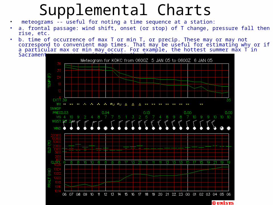
Supplemental Charts• meteograms -- useful for noting a time sequence at a station:• a. frontal passage: wind shift, onset (or stop) of T change, pressure fall then rise, etc.• b. time of occurrence of max T or min T, or precip. These may or may not correspond to

convenient map times. That may be useful for estimating why or if a particular max or min may occur. For example, the hottest summer max T in Sacramento may occur quite late in the day.

End of Current Weather

Storage