ATFM 2016

User Guide

FLIM / FRET …………………… 3

FRAP ……………………………… 13

SIM ……………………………….. 23

STED ……………………………… 37

The workshop is organized in the framework of the Czech-BioImaging

research infrastructure supported by MEYS (LM2015062)

ATFM 2016

2

ATFM 2016 – general partners

Distributor of Thermo Scientific and Leica-microsystems instruments

ATFM 2016

3

FLIM / FRET

Marie Olšinová / Aleš Benda

ATFM 2016

4

01 FLIM - FRET – PRINCIPLE AND THEORY

FRET introduction

Förster resonance energy transfer (FRET) is a non-radiative energy transfer between two fluorophores,

named a donor and an acceptor, meeting several criteria (Figure 1): the fluorophores are in a close

proximity, their mutual orientation is favorable (meaning that their transition dipole moments are not

perpendicular) and the donor emission and the acceptor excitation spectra overlap. In particular, the

proximity criterion indicates the most common application of FRET: studying molecular interactions.

Another application is microenvironment sensing through FRET based sensors.

Figure 1 A demonstration of necessary criteria for FRET to happen. a. a donor emission spectrum and

an acceptor excitation spectrum overlap; b. a proximity of the donor and the acceptor; c. an orientation

of the donor and the acceptor. Adopted from Broussard et al.1

Energy is radiationlessly transferred between the excited fluorescent molecule (donor) and the

acceptor molecule through a dipole-dipole coupling. The donor molecule returns to the ground state

and the acceptor molecule gets to the excited state, which is followed by a red photon emission. FRET

manifests itself by a signal reduction in the donor channel, signal increase in the acceptor channel, or

by a reduction of the donor lifetime. Efficiency of the energy transfer EFRET depends mainly on the

distance between the donor and the acceptor r (Figure 2), for freely rotating donor and/or acceptor

fluorophores can be described by:

ATFM 2016

5

𝐸𝐹𝑅𝐸𝑇 =𝑅06

𝑅06 + 𝑟6

Where 𝑅0 is Förster radius indicating a distance at which FRET efficiency decreases to 50%. For the

most used FRET pairs, e.g. CFP and YFP, 𝑅0 is around 5 nm meaning that FRET is detectable up to the

distance of about 10 nm. 𝑅0 depends on the quantum yield and the excited state lifetime of the donor

in the absence of the acceptor, the refractive index of the medium, the spectral overlap of the donor

and the acceptor and the factor describing a relative orientation of the donor and acceptor dipoles.

𝑅0might be calculated directly (for details please see e.g. Lakowicz2).

Figure 2 The dependence of FRET efficiency on the

donor-acceptor distance. Adopted from

Piston&Kremers.3

Different types of microscopes can be used to detect and quantify FRET, applying several different

methodological approaches. For our hands-on experiments we will focus on a confocal microscope,

which is a versatile tool enabling to apply any of the three most common methodologies used3:

1) Sensitized emission

The sensitized emission is an intensity based approach that compares fluorescence intensities in

the donor and the acceptor channels while exciting the donor only. If FRET occurs, the intensity in

the acceptor channel increases and simultaneously decreases in the donor channel. On contrary,

FRET absence shows itself as a high signal in the donor channel and a low signal in the acceptor

channel. Although the idea is straightforward, a practical realization is often complicated due to

the spectral properties of the donor and the acceptor. The donor emission is usually seen also in

the acceptor channel (a spectral bleed-through or cross-talk) and the acceptor could be directly

excited by the donor excitation wavelength (a direct excitation). An absolute quantification of FRET

efficiency thus requires a number of careful control experiments. Moreover, for direct interaction

or FRET sensor based studies an unknown or variable labeling ratio of the molecules of interest by

both fluorophores complicates the analysis (in simple words some molecules are missing the

acceptor). For indirect colocalization (aggregation) studies the complication comes from varying

concentrations of donor and/or acceptor molecules (the higher the acceptor concentration the

higher the FRET). These inherent uncertainties can be caused by an unstable fluorescence protein

expression, different FP maturation rates, varying efficiency of external fluorophore linking

reactions, or simply by photobleaching. A low average FRET efficiency might mean both longer

distances between the donor and the acceptor or just a low abundance of complete FRET pairs or

low acceptor concentrations.

2) FLIM-FRET

ATFM 2016

6

FLIM-FRET is the excited state lifetime based FRET that monitors changes in the donor excited state

lifetime in the presence and the absence of the acceptor. The excited state fluorescence lifetime

is a characteristic time that molecule spends on average in the excited state before a photon

emission occurs, typically in range of ns. It is also environment specific. If FRET occurs, the donor

returns to the ground state without a photon emission causing a reduction of the donor excited

state lifetime. A comparison of the donor fluorescence lifetime in the presence and the absence

of the acceptor provides information about the FRET efficiency EFLIM-FRET.

𝐸𝐹𝐿𝐼𝑀−𝐹𝑅𝐸𝑇 = 1 −𝜏𝐷𝐴𝜏𝐷

Where τDA resp. τD is the donor lifetime in the presence, resp. the absence of the acceptor. The

main advantage of the lifetime based approach is that it is not prone to spectral and concentrations

artefacts. On the other hand it is more demanding in respect to the microscopy equipment.

3) Anisotropy imaging (homo-FRET)

FRET can occur also between two identical fluorophores provided their excitation and emission

spectra overlap, which is often the case. This so-called homo-FRET is not detectable by changes in

spectral or excited state lifetime properties of the sample. The only way how to detect it is to

follow the fluorescence anisotropy (polarization). As the energy migrates from one fluorophore to

another, which is on average oriented slightly differently that the original acceptor, the orientation

of the emission dipole is more different to the orientation of the original absorption dipole, which

decreases the overall anisotropy. To precisely measure the anisotropy the instrument must allow

to split the signal according to the photon polarization onto two detectors, usually by using a

polarization splitting cube. This method is not covered in our hands-on experiments.

One of the popular and powerful ways to obtain a negative reference is an acceptor

photobleaching method. The acceptor photobleaching (or donor dequenching) is used for both

intensity and lifetime based FRET. As was already mentioned, the donor signal is reduced

(quenched) in the presence of the acceptor by an energy transfer. If the acceptor is disabled

(photobleached), the original donor intensity is restored. A comparison of the donor signal (both

the intensity and the excited state lifetime) at sample containing both the donor and the acceptor

before and after the acceptor photobleaching provides information about the FRET efficiency. This

approach is free of signal bleedthrough and might be performed during a single measurement. The

obvious disadvantage is that it can be done only once and only in fixed cells (a diffusion of the

acceptor to the bleached area might distort the result). In order to perform these experiments,

one must ensure that the donor is not destructed by the acceptor photobleaching and that the

acceptor signal fully diminishes – this takes time (minutes) and prolongs the experiment. Despite

the mentioned drawback, it is worthy to perform the acceptor photobleaching at least in the end

of the experiment session.

What is FLIM?

Fluorescence Lifetime Imaging Microscopy (FLIM) is a method that enables to measure fluorophores

excited state lifetimes at individual image pixels. As the lifetime is fluorophore and environment

specific, FLIM can be used to e.g. local environment sensing, detection of molecular interactions (FRET)

or to discriminate among multiple labels.4

ATFM 2016

7

It is probably worth to repeat that the excited state lifetime is the characteristic average time

molecules remains in the excited state after a photon absorption and before a photon emission. The

emphasis is on the words “characteristic average” implying that the photon emission is a random

process. A photon can be emitted 0.5 ns after the excitation but also 6 ns after the excitation. In order

to get the average value, several thousands of photons need to be detected by time correlated single

photon counting (TCSPC). TCSPC measures time between the pulsed excitation (start of the

measurement) and the photon detection (end of the measurement) (Figure 3a). A histogram of arrival

times provides the temporal record of fluorescence decay (Figure 3b).

A real measurement of the photon arrival times is accompanied by some uncertainty coming from

electronics limitations. The time for the photon detection and its conversion to an electric signal could

take tens to hundreds of ps mainly depending on the detector type. Next, the laser pulse width is also

usually tens to hundreds of picoseconds. All these factors influence the shape of the measured decay.

The way how the infinitely short fluorescence decay is detected by a microscope is represented by

Instrument Response Function (IRF). IRF is analogous to the point spread function (PSF), just IRF is in

time domain and PSF in spatial domain. This means that every measured decay is partly distorted by

IRF especially at short decay times. A reconstruction of the “true decay” is possible by an iterative

reconvolution method. Another way is to study events only on the longer timescale by excluding the

IRF time window (a tail-fitting approach).

Figure 3. a. A measurement of time interval between the

laser pulse and the photon detection by TCSPC. Image

adopted from Wahl.5 b. A schematic representation of a

photon arrival times histogram forming the fluorescence

decay.

Decay analysis

ATFM 2016

8

A fluorescence decay I(t) is mathematically described by mono or multi exponential functions. For

simplicity we will consider a theoretical decay not influenced by IRF. Fitting of this decay to the mono-

or multi-exponential model provides characteristics decay times i.

𝐼(𝑡) =∑𝛼𝑖 𝑒−𝑡/𝜏𝑖

i are amplitudes of components at time t = 0. There are also approaches that do not a priori assume

the number of exponentials, e.g. phasor plot representation6, but because of their complexity we will

not go into the details.

The fitted parameters provide us with more details about the system. Consider e.g. the situation that

not every donor is bound to the acceptor. Then the decay of the donor at presence of the acceptor

would contain at least two exponentials. The first decay time would represent a lifetime of the donor

in the presence of the acceptor, the second one the donor in the absence of the acceptor. A

comparison of amplitudes related to the mentioned lifetimes could provide information about the

binding stoichiometry. Another situation: If the resulting decay is multiexponential, it might indicate

that the donor and the acceptor distances vary. In order to describe such a complicated decay, we can

calculate the average lifetime based on amplitude weighting.

𝜏𝐴𝑚𝑝𝑙 =∑ 𝛼𝑖𝜏𝑖𝑖

∑ 𝛼𝑖𝑖

This amplitude weighted lifetime is used for FRET efficiency calculation.

02 FRET – PRACTICAL PART

02.1 Equipment Confocal inverted microscope Leica SP8 SMD-FLIM

An inverted microscope Dmi8 AFC Bino with a laser scanning confocal head, a motorized microscope stage with a Super Z-galvo scanning insert for fast and precise Z movement, HW autofocus control, transmitted light equipment including a transmitted light PMT, differential interference contrast available for 63x objectives. A pulsed excitation by 405 nm laser or white light laser (470 nm – 670 nm). The confocal head is equipped with two standard PMT detectors and two highly sensitive HyD detectors suitable for FLIM with a time resolved gating option. The system is equipped with a TCSPC unit (HydraHarp400, Picoquant) enabling time resolved experiments such as FLIM or FCS. Illumination: Epifluorescence: CoolLED p300 (fluorescence filter cubes DAPI, FITC, RHOD, Cy5) Excitation lasers: A pulsed White Light Laser (WLL2) 470 nm-670 nm, the actual wavelength selectable with 1 nm step, up to 8 parallel laser lines, up to 1.5 mW per each line, the basic frequency is 80 MHz, dividable to 40 MHz and lower. The laser wavelength and intensity is controlled by a combination of AOTF and AOBS.

A pulsed 405 nm laser diode, laser power at sample position up to 83 W, frequency 40 MHz and lower (down to 312,5 kHz). Objectives: HC PL APO 10x/0.40 HC PL APO 20x/0.75 CS2

ATFM 2016

9

HC PL APO 63x/1.2 W Corr CS2 HC PL APO 63x/1.4 Oil CS2 Confocal scanning head: Leica TCS SP8. The laser excitation wavelength is selected and intensity regulated by an acousto-optical tunable filter (AOTF). The excitation and emission light is separated by an acousto-optical beam splitter (AOBS). Conventional FOV SP8 scanner, with maximal sampling 8192x8192px, speed 1-1800 Hz (7fps@512x512 px), hardware zoom 0.75x-48x, spectrally tunable detection (a simultaneous detection of four different channels via a prism-based dispersive element), 2x PMT detectors (400-800nm), 2x HyD detectors (GaAsP, 400 – 720 nm) for FLIM (time-gating possible), 1x TLD detector for transmitted light. TCSPC unit: HydraHarp400. Two channels available. Enables to detect photon arrival times with respect to the beginning of the experiment and the excitation pulse and the channel in which the photon was registered (TTTR mode). In combination with a scanner controller, a histogram acquisition at different image positions is available. Histogramming measurement ranges from 65 ns to 2.19 s (depending on the chosen time bin resolution: 1, 2, 4, ..., 33 554 432 ps). Software: LAS X for image acquisition and Symphotime64 for image acquisition and analysis. The microscope is equipped with the OKOlab incubation system for live cell imaging (regulation of

temperature and CO2 level).

02.2 Aim

To acquire and analyze FLIM images and to implement FLIM in FRET experiments.

02.3 Sample preparation

For FLIM-FRET imaging, the structures of interest need to be labelled by donor and acceptor molecules.

There is a great variety of fluorophores that might be used. Not only protein-protein pairs, but also

organic dyes pairs can be employed (𝑹𝟎 of different organic dyes are often provided by companies7, it

can serve as a basic tool for dye pair selection). To mention just few protein-protein pairs: CFP-YFP,

GFP-mCherry, GFP-mRFP, Cerulean-YFP, BFP-GPF, mClover-mRuby and many more. Different protein

based FRET pairs were compared and reviewed at e.g. Bajar et al8. If possible, please prepare three

samples: unlabeled cells, cells labeled with the donor only, cells labeled with both the donor and the

acceptor.

Preparation of training sample for hands-on session: FLIM will be measured in HT1080 cells (human

fibrosarcoma) transfected with Src-biosensor. Src is localised at cytoplasm, accumulates in leading

edge, in focal adhesions, and in invadopodia. The biosensor consists of full-length Src kinase, into which

mTurquoise (donor) and mCitrine (acceptor) variants of GFP are inserted. During the training we will

try to distinguish between the compact and loose conformation of Src-biosensor. The distance

between the donor and the acceptor is shorter for the compact conformation resulting in higher FRET

efficiency.

Cells were transiently transfected, sorted and grown on Mattek Petri dishes. For purpose of this

practical course cells were fixed with 4% PFA and kept in PBS at 4°C. As a negative control donor-only

ATFM 2016

10

containing cells will be measured. The measurement will consist of: 1) FLIM measurements of donor

signal in the whole cell; 2) an acceptor bleaching of selected part of the cell; 3) FLIM measurements of

donor signal in both bleached and unbleached areas of the cell; 4) a comparison of the obtained data.

02.4 Data acquisition

Setup the microscope for FLIM-FRET measurements on the sample containing both the donor and the

acceptor. Select the laser wavelengths and frequency, objective, pinhole, emission detection ranges

for HyD detectors, line/frame acquisition and line/frame accumulation/averaging. Adjust laser

intensities, image size, scanning speed and zoom. Keep the same acquisition settings during the

measurement of both your sample and controls.

Check the unlabelled sample for autofluorescence.

Acquire intensity images of the donor and the acceptor. To be sure that both structures are present.

Acquire lifetime image of the donor in the presence of the acceptor. A general rule for FLIM data

acquisition: To avoid artefacts, a maximum count rate per pixel (is different from the average signal

per image) should not exceed 10% of the laser repetition.

Acquire lifetime image of the donor in the absence of the acceptor. Either prepare a sample where just

the donor structure would be labelled. Or bleach the acceptor and measure the donor lifetime in the

bleached area (applicable only for fixed cells or rigid structure with negligible diffusion).

Training sample: Follow the general workflow. The lifetime image of the donor in the absence of the

acceptor will be measured after the acceptor photobleaching. To bleach a selected part of the cell, a

maximal laser intensity is needed, the bleaching is stopped when the acceptor intensity drops at least

to 10% of its initial value. A sufficient time bin for our TCSPC system is 32 ps.

02.5 Data analysis

Load the data to the software that can read the time-resolved images (e.g. Symphotime64). Select the

region of interest for the donor only area, select the fitting range based on the fitting method (n-

Exponential Tailfit or n-Exponential Reconvolution), start with the mono-exponential fit. If insufficient,

go for the two-exponential fit. The fit is good if residual values are low and without periodic pattern

and χ2 close to one. Repeat the procedure for the donor-acceptor area. Compare the shape of decays

and fitted amplitude weighted lifetimes.

03 Literature 1. Broussard, J. A., Rappaz, B., Webb, D. J. & Brown, C. M. Fluorescence resonance energy

transfer microscopy as demonstrated by measuring the activation of the serine/threonine kinase Akt. Nat. Protoc. 8, 265–81 (2013).

2. Lakowicz, J. R. Principles of Fluorescence Spectroscopy Principles of Fluorescence Spectroscopy. (Springer, 2006). doi:10.1007/978-0-387-46312-4

3. Piston, D. W. & Kremers, G.-J. Fluorescent protein FRET: the good, the bad and the ugly. Trends Biochem. Sci. 32, 407–414 (2007).

ATFM 2016

11

4. Trautmann, Susanne Buschmann, V., Orthaus, S., Koberling, F., Otrmann, U. & Erdmann, R. Fluorescence Lifetime Imaging (FLIM) in Confocal Microscopy Applications: An Overview. Application Note PicoQuant 1–14 (2013). at <https://www.picoquant.com/images/uploads/page/files/7350/appnote_flim_overview.pdf>

5. Wahl, M. Time-correlated single photon counting. Technical Note PicoQuant 1–14 (2014). doi:10.1016/0022-2313(89)90051-3

6. Digman, M. a, Caiolfa, V. R., Zamai, M. & Gratton, E. The phasor approach to fluorescence lifetime imaging analysis. Biophys. J. 94, L14-6 (2007).

7. ATTO TEC GmbH. Förster-radius of selected ATTO-dye pairs. 15–16 (2016). doi:10.1139/o05-906

8. Bajar, B., Wang, E., Zhang, S., Lin, M. & Chu, J. A Guide to Fluorescent Protein FRET Pairs. Sensors 16, 1488 (2016).

ATFM 2016

12

ATFM 2016

13

FRAP

Michaela Efenberková (Blažíková)

ATFM 2016

14

01 FRAP – PRINCIPLE AND THEORY

The methods that allow us to study and compare dynamics of molecules within living cells are

based on perturbation of the steady-state fluorescence distribution in a selected region of the

specimen and observation of fluorescence recovery towards the steady-state. They include

the techniques based on photobleaching, photoactivation and photoconversion. The

photobleaching methods involve Fluorescence Recovery After Photobleaching (FRAP),

Fluorescence Loss In Photobleaching (FLIP) and inverse FRAP (iFRAP).

In FRAP experiment, first a selected region of interest (ROI) in the sample is selectively photobleached by a brief exposure to an intense focused laser beam. The fluorophores in the bleached spot are photochemically altered and they are permanently unable to fluoresce. The subsequent recovery of fluorescence intensity in the same ROI is caused by replenishment of intact fluorophore in the bleached spot by transport from the surrounding unbleached regions, see Figure 1. The recovery of the fluorescence is monitored by the same, but attenuated, laser beam.

Figure 1. Principle of FRAP and example of recovery curve In the simplest case of pure diffusion of particles, the diffusion coefficient D can be calculated according to Stokes-Einstein equation:

𝐷 =𝑘𝑇

6𝜋𝜂𝑅 Eq.1

ATFM 2016

15

where k is Boltzmann constant, T represents absolute temperature, ƞ viscosity of the solution and R hydrodynamic radius of the particle. It is thus clear that the mobility of a molecule in the cellular environment is affected by

size of the molecule

cellular environment (viscosity, temperature)

protein-protein interactions and binding to other macromolecules

flow or active transport.

01.1 Qualitative analysis

The first FRAP experiments developed in 1970’s were able to investigate 2-dimensional lateral movement monitored by a laser beam of Gaussian intensity profile, and of uniform circular disc profile [1]. Later models investigate the motion of the molecules also in 3D (3D diffusion can be inspected using multi-photon FRAP), however still under defined specific conditions. This exercise is aimed on 2D models. The simplest approximation of the fluorescence recovery curve F is a single exponential growth function

𝐹 = 𝐹0 +𝑀(1 − 𝑒−𝜏𝑡) Eq. 2

where F0 is the initial value of fluorescence intensity after photobleaching, t represents time and M and τ are coefficients of the exponential function. Using this single exponential it is possible to fit the recovery curve and obtain 2 basic qualitative parameters - immobile fraction and half-time, see Figure 2. Immobile fraction I corresponds to (1-M), where M is the mobile fraction equal to % of the maximum reached intensity and half-time τ1/2

𝜏1/2 =ln(0.5)

−𝜏 Eq. 3

Figure 2. Basic qualitative parameters of the recovery curve

ATFM 2016

16

In the case the single exponential does not fit the curve sufficiently, which can be easily determined e.g. using residuals (difference between the observed value and the estimated value of the quantity of interest) that should be randomly distributed around zero, a different function might be used to fit the curve and obtain the desired parameters (immobile fraction and half-time), as is shown in Figure 3. The most common is the double exponential function

𝐹 = 𝐹0 + 𝐶1(1 − 𝑒−𝜏1𝑡) + 𝐶2(1 − 𝑒−𝜏2𝑡) Eq. 4

where C1, C2 and τ1, τ2 are coefficients of the double exponential function and do not necessarily represent two fractions of fluorescently labeled particles (only immobile fraction and half-time can be compared using such qualitative analysis).

Figure 3. Simple and double exponential fit with residuals It is usually necessary to correct the FRAP curves for photobleaching before analyzing them (by acquiring the fluorescence intensity in areas where the fluorophores were not photobleached). For further comparisons it is also necessary to normalize the FRAP curves (set intensity before photobleaching equal to 1).

FRAP is then used to:

compare the motion of two different fluorescently labeled molecules

compare the motion of the same molecule in different region/structure

compare the motion of the same molecule before and after treatment.

For example faster recovery after the treatment (when compared to the situation before the treatment) can indicate lack of interaction or spatial restriction, conformational change of the

ATFM 2016

17

protein that is now diffusing faster; higher immobile fraction can indicate a new interaction or spatial restriction, etc.

01.2 Quantitative analysis

To obtain more information about the movement of the labeled molecules, more complicated functions and models have to be used. An appropriate model can be chosen according to the role of diffusion. This can be investigated experimentally. When diffusion plays a substantial role, the recovery exhibits a spatial dependence, whereas if only binding is measured then the rate of recovery should not change as a function of either bleach spot size or location within the bleach spot [2]. Bleaching can be performed with different spot sizes or the fluorescence profile over time can be recorded across the bleach spot to check the role of diffusion.

The reaction-limited recovery reflects the situation when diffusion is very fast compared to binding and to the timescale of FRAP experiment and a single binding reaction dominates. The reaction is:

𝑆𝑓 + 𝐵

𝑘𝑜𝑛→

𝑘𝑜𝑓𝑓← 𝐶𝑓 Eq .5

where Sf is the free fluorescently labeled solute molecule, B its unlabeled binding partner, Cf their fluorescent complex, and kon and koff the on and off rates of binding. The fluorescent signal in FRAP experiment is a contribution of both free molecules and molecules in the complex. The recovery curve can be then approximated using a single exponential function [3]

𝐹 = 1 − 𝐶𝑒𝑞𝑒−𝑘𝑜𝑓𝑓𝑡 ,𝐶𝑒𝑞 =

𝑘𝑜𝑛∗

𝑘𝑜𝑛∗ +𝑘𝑜𝑓𝑓

Eq. 6

where koff and kon*are off- and pseudo-on rates, respectively; these can be calculated as a result of the analysis. Pseudo-on rate constant is given by kon* = kon[B], [B] being the concentration of the unlabeled binding partner that is constant throughout the FRAP experiment. There is also a possibility to take into account 2 binding reactions, the approximation of the FRAP recovery curve then corresponds to double exponential function (similarly to Eq. 4).

In the case of diffusion-limited recovery we are able to calculate the effective diffusion coefficient Deff, that is equal to diffusion coefficient D in the case of pure diffusion of the molecules (where there are nearly no interactions present and most of the fluorescent molecules are free). Effective diffusion coefficient is an approximation of the diffusion coefficient in the case of diffusion-limited recovery, when reaction process is much faster than diffusion (kon<<koff), and reflects the mean squared displacement explored by the proteins through a random walk over time [4]

𝐹 = 𝑒−𝜏𝐷2𝑡 (𝐼0 (

𝜏𝐷

2𝑡) + 𝐼1 (

𝜏𝐷

2𝑡)),𝜏𝐷 = 𝑤2/𝐷𝑒𝑓𝑓 Eq .7

ATFM 2016

18

where I0 and I1 are modified Bessel functions of the first kind, w is the bleach spot radius and Deff = D/(1 + kon*/koff) the effective diffusion coefficient.

The full reaction-diffusion model is an approximation of the combination of effective diffusion and one binding reaction. The Laplace transform of the FRAP recovery curve then corresponds to [5]

𝐹(𝑝)̅̅ ̅̅ ̅̅ = (1−𝐶𝑒𝑞

𝑝) (2𝐾1(𝑞𝑤)𝐼1(𝑞𝑤)) (1 +

𝑘𝑜𝑛∗

𝑝+𝑘𝑜𝑓𝑓) ,𝑞 = (

𝑝

𝐷𝑒𝑓𝑓) (1 +

𝑘𝑜𝑛∗

𝑝+𝑘𝑜𝑓𝑓)Eq. 8

where I1 and K1 are modified Bessel function of the first and second kind. The final solution is represented as inverse Laplace transform of the Eq.8. As a results the effective diffusion coefficient, off-rate and pseudo-on rate can be calculated.

A modification of the full model for two binding reactions and accounting for the boundary effects (e.g. nucleus) are also possible.

The models have to be selected carefully with some prior knowledge about the processes using different experimental methods. The models can then determine:

how fast the molecule is moving

if the molecule is bound to one or more surrounding structures

if it is freely diffusing or the movement is restricted by surrounding structures.

For further information about modelling approaches see [6, 7]. For examples of FRAP analysis and results using the above mentioned modeling approaches see [8, 9]. There is a possibility to construct more complicated models of specific interactions between molecules using compartmental analysis. A multi-compartment model is a type of mathematical model used for describing the way materials or energies are transmitted among the compartments of a system. Each compartment is assumed to be a homogeneous entity within which the entities being modelled are equivalent (e.g. concentration). For an example of such approach see [10].

ATFM 2016

19

02 FRAP – PRACTICAL PART

02.1 Equipment

Microscope: Delta Vision Core

Software for image and data analysis: FIJI, Matlab (MathWorks), MS Excel

Instructor: Michaela Blažíková, PhD

02.2 Aims

To analyze and compare the movement of several fluorescently labeled molecules using

FRAP. Measure FRAP experiments in different cell areas and compartments. Analyze the

images to obtain recovery curves and determine qualitative and quantitative parameters

using different models. Compare the results. Try out photoactivation and photoconversion

experiments.

02.2 Sample preparation

In the practical part, FRAP will be measured in nuclei of human HeLa cells that stably express GFP-tagged spliceosomal proteins under endogenous promoter from recombineered BACs. The cells are maintained in DMEM containing 10% serum and 1% antibiotics. 24 hours before the experiment, cells are transferred on 3 cm glass-bottomed petri-dish. The day of the experiment, cells are washed with PBS and incubated in imaging medium without phenol red. This step is important because phenol red increases background fluorescence. Photobleaching will be performed in different sub-nuclear compartments and protein dynamics in these compartments will be compared.

For photoactivation and photoconversion experiments, HeLa cells are transfected with plasmids encoding photoactivatable (PA) GFP or Dendra, respectively. 24 hours before the experiment, cells in 3 cm glass-bottomed petri-dish are treated with 2 µg DNA mixed with Lipofectamine transfection reagent and DMEM; transfection is done according to manufacturer’s protocol. The day of the experiment, cells are washed and incubated in imaging medium as described above.

02.3 Data acquisition

Every FRAP experiment is unique and depends on biological molecule to be studied, the

fluorochrome used, the geometry of the specimen and microscope set-up. Here, we present

a set of useful guidelines that should be followed in most photobleaching experiments.

Requirements for FRAP:

1. microscope that allows fast recording of fluorescence intensity over time,

2. system that allows local increase of excitation light to perform the bleach.

ATFM 2016

20

FRAP experiment will be demonstrated using wide-field fluorescence microscope Olympus

IX70 equipped with lasers which fulfills both of these requirements.

FRAP measurement details:

- Objective – usually 60x or 100x with a high numerical aperture, but for some

applications a low numerical aperture objective to ensure cylindrical and homogenous

bleach in depth should be considered

- Pinhole – adjusted according to the thickness of the studied structure/compartment

(not applicable for a wide-field microscope)

- Pixel size – adjusted according to the speed required (not applicable for wide-field

microscope)

- Time intervals – should provide a good resolution of the dynamic part of the

fluorescence redistribution

- determine time of the first image after photobleaching (sa fast as possible)

- total time of acquisition - it is essential to clearly see the plateau at the end of the

recovery if immobile fraction and half-time of the recovery want to be analyzed; the

gold rule is to acquire twice as long as it took to reach the plateau

- approximately 10 images should be acquired before the bleach, it serves a reference

for the percentage of the recovery, essential for the quantitative analysis

- Shape and size of the photobleached area – depends on the specimen

- Bleaching efficiency – optimized experimentally on a fixed sample – should be > 50%

- laser power set to maximum, number of iterations kept the same for all experiment

repetitions; it affects the recovery profile

- Intensity of the laser for image acquisition after photobleaching – to prevent

photobleaching during recovery

02.4 Data analysis

Acquired images will be processed using FIJI to obtain FRAP recovery curves that will be

analyzed using Matlab scripts.

I. Using FIJI obtain intensities in the bleached region (ROI), background and area for

correction of photobleaching during fluorescence recovery (far from the bleached

region)

II. Normalize fluorescence intensities in Excel. There is also possibility to use FIJI script to

obtain intensities and perform normalization of the FRAP curves

(http://fiji.sc/Analyze_FRAP_movies_with_a_Jython_script)

III. Qualitative analysis using Matlab scripts (will be presented during the exercise)

a. Fit the recovery curves by single exponential function and estimate

mobile/immobile fraction and recovery half-time, according to Eq. 2 and 3

b. Fit the recovery curve by double exponential function, according to Eq. 4

c. Compare the results

IV. Quantitative analysis using Matlab scripts (will be presented during the exercise)

ATFM 2016

21

a. Choose an appropriate model according to the role of diffusion and estimate

diffusion coefficient and binding rates

b. Fit the recovery curve with the chosen models, according to Eq. 6, 7 or 8

c. Compare the results

When comparing and summarizing the final results, one has to be careful and aware of the

assumptions applied to most of the models [2]:

infinite homogeneous media

absence of flow or other type of directed motion

free and unrestricted diffusion

initial uniform distribution of fluorophores

absence of diffusion during bleaching.

There are also alternative techniques to determine molecular dynamics, such as single-particle tracking include (SPT), fluorescence correlation spectroscopy (FCS), image correlation spectroscopy (ICS) and and nuclear magnetic resonance diffusometry (NMRd). These can be used in case when FRAP cannot be applied, due to e.g. too fast or too slow diffusion of molecules undetectable by FRAP, or as complementary methods to FRAP.

02.5 Literature

1. Axelrod, D., et al., Mobility measurement by analysis of fluorescence photobleaching recovery kinetics. Biophys J, 1976. 16(9): p. 1055-69.

2. Loren, N., et al., Fluorescence recovery after photobleaching in material and life sciences: putting theory into practice. Q Rev Biophys, 2015. 48(3): p. 323-87.

3. Sprague, B.L., et al., Analysis of binding reactions by fluorescence recovery after photobleaching. Biophys J, 2004. 86(6): p. 3473-95.

4. Soumpasis, D.M., Theoretical analysis of fluorescence photobleaching recovery experiments. Biophys J, 1983. 41(1): p. 95-7.

5. Sprague, B.L., et al., Analysis of binding at a single spatially localized cluster of binding sites by fluorescence recovery after photobleaching. Biophysical Journal, 2006. 91(4): p. 1169-1191.

6. McNally, J.G., Quantitative FRAP in analysis of molecular binding dynamics in vivo. Methods Cell Biol, 2008. 85: p. 329-51.

7. Mueller, F., et al., FRAP and kinetic modeling in the analysis of nuclear protein dynamics: what do we really know? Curr Opin Cell Biol, 2010. 22(3): p. 403-11.

8. Phair, R.D. and T. Misteli, Kinetic modelling approaches to in vivo imaging. Nat Rev Mol Cell Biol, 2001. 2(12): p. 898-907.

9. Huranova, M., et al., The differential interaction of snRNPs with pre-mRNA reveals splicing kinetics in living cells. J Cell Biol, 2010. 191(1): p. 75-86.

10. Novotny, I., et al., In vivo kinetics of U4/U6.U5 tri-snRNP formation in Cajal bodies. Mol Biol Cell, 2011. 22(4): p. 513-23.

ATFM 2016

22

ATFM 2016

23

SIM

Jindřiška Fišerová / Martin Čapek

ATFM 2016

24

01 STRUCTURED ILLUMINATION MICROSCOPY – SIM – PRINCIPLE AND THEORY

Structured illumination microscopy (SIM) is one of super-resolution light microscopy

techniques that allows doubling the resolution in comparison with wide-field microscopy. This

might not seem that stunning when acknowledging that other super resolution techniques

(e.g., STED, STORM) can increase the resolution up to tens of nanometres. However, the great

advantage of SIM is the compatibility with live-cell imaging. Further, in 3D-SIM, increasing the

axial resolution results in substantial improvement of the localisation volume. And finally,

since quite large field of view can be captured, the object can be observed within the cellular

context.

In SIM the sample is excited by a non-uniform (or patterned) wide-field illumination. The

patterned illumination is achieved by passing the laser light through an optical grating, which

generates a stripe-shaped interference illumination pattern. The pattern is used to illuminate

the sample in three angles and five shifts (see Fig. 1).

Figure 1. Principle of the SIM microscopy (adopted from Shermelleh et al. 2010)

The interference of the illumination pattern and the object structures bellow the diffraction

limit of the particular wavelength (in other words below the resolution of a wide-field

microscope and, therefore, impossible to detect by wide-field) generates so called Moiré

fringes. Otherwise unobservable sample information can be computed from the Moiré fringes

and computationally restored. The process of computing a final image, i.e. the reconstruction

of the image, results in generating a high-resolution SIM image with doubled resolution in xy

as well as in z compared with the wide-field. More details on the optics and physics behind

can passionate readers find in the recommended literature bellow.

ATFM 2016

25

The Point Spread Function. An important characteristic of a microscope is the Point Spread

Function (PSF). It describes the response of the imaging system to a point source. In ideal case,

the response of the system on a bright point should be again a bright point. In real practice,

however, the response of a point is a blurred object, both in xy (Fig. 2) and xz (Fig. 3) plane [7].

Figure 2. 3D visualization of PSF intensities of microscopes in xy plane in space domain and

corresponding OTFs in kxky plane in frequency domain with increasing quality of objectives, i.e.

with increasing their NA (=numerical aperture). The emission wavelengths were 510 nm.

Notice that wider PSF corresponds to narrower OTF and vice versa.

Figure 3. Axial slice (xz plane) of the PSF for objective NA = 1.2 and λem = 510 nm. Intensity

shown in pseudo-color in logarithmic scale. Axial axis is along vertical direction. Scale bar 500

nm.

ATFM 2016

26

Fourier transform and Optical Transfer Function. The basic concept of reconstruction of

super-resolved images from SIM raw data can be described through conversion of images to

the frequency domain by using the Fourier transform.

The Fourier transform of a function of time, e.g. an image, is a function of frequency that

represents the amount of that frequency present in the image. The Fourier transform is called

the frequency domain representation of the original image

(https://en.wikipedia.org/wiki/Fourier_transform).

The Fourier transform of the PSF is called the Optical Transfer Function (OTF) (Eq. 1). There

are three OTFs computed for objectives with different NA shown in Fig. 2a-c above. We

observe that a localization of the PSF in real space (narrow peak) leads to a delocalization of

the OTF (broad peak) in Fourier space and vice versa. In general, the OTF is always zero for

high spatial frequencies of the Fourier transformation. In other words the microscopy system

acts as a low pass filter (transmitting low frequencies only) for spatial frequencies in the

Fourier transform. A comparison of the OTFs computed for objectives with different NA is

shown in Fig. 4 (d-f). An absence of Fourier components along the axial direction (kz axis) is

the so called ”missing cone” problem – a red cone drawn in the image, which results in worse

resolution and, consequently, worse optical sectioning of structures in z.

ATFM 2016

27

𝐹{𝑃𝑆𝐹(𝑟)}(�⃗⃗�) = 𝑂𝑇𝐹(�⃗⃗�);𝑟 … 𝑠𝑝𝑎𝑐𝑒𝑣𝑒𝑐𝑡𝑜𝑟, �⃗⃗� … 𝑓𝑟𝑒𝑞𝑢𝑒𝑛𝑐𝑦𝑣𝑒𝑐𝑡𝑜𝑟 (1)

Figure 4: Axial slices (xz plane) of the PSF for water immersion objectives with numerical

apertures (a) NA = 0.3, (b) NA = 0.9 and (c) NA = 1.2. λem = 510 nm. Scale bar 3 µm.

Corresponding OTF (kxkz plane) displayed in (d-f). The z-axis is along the vertical direction.

Notice again that better shaped PSF corresponds to broader OTF, which means that objectives

with higher NA can transfer higher frequencies, i.e. more details. A ”missing cone” problem is

demonstrated in (f).

ATFM 2016

28

The concept of resolution improvement by structured illumination. To understand the following

explanations it is useful to know that Fourier transform of a constant signal contains one peak

at zero frequency and of a sinusoid with spatial frequency 2k contains two extra peaks at -2k

and 2k (Fig. 5).

Figure 5: Constant signal (e.g., white constant image), sinusoid (e.g., stripes in an image) and

their counterparts in the Fourier space.

When the Fourier transform of the object (Fig. 6a) is multiplied with the OTF, all frequency

components outside the support of the OTF are lost (Fig. 6b). When the sample is multiplied

with a sinusoidal grating pattern, i.e. illuminated using a structured pattern creating a Moiré,

two extra peaks at -2k and 2k corresponding to the sinusoid are created in Fourier space with

the same information attached to each peak (Fig. 6c). After multiplication with the OTF again,

there is now information inside the OTF that would have normally been lost (Fig. 6d). If the

ATFM 2016

29

information attached to the side components can be separated and moved to coincide with

the middle peak, extra frequencies can be recovered (Fig. 6e). After shifting both side

components (Fig. 6f) they are combined with the middle peak using weighted averaging (Fig.

6g). The final image, obtained by inverse Fourier transform, now contains more frequencies

and thus has better resolution.

Figure 6: Resolution improvement by structured illumination described in the Fourier space, for

simplicity using the Fourier transform of 1D signal.

(a) (b)

(c) (d)

(e) (f) (g)

ATFM 2016

30

Illumination pattern projected on a 2D sample (simulated images). Four orientations of the

illumination pattern are projected on the sample using orientations of 0°, 90°, 45° and 135°

(Fig. 7a-d). Corresponding Fourier transforms (in kxky frequency domain; amplitude at the

given frequency is coded by intensity) are in Fig. 7e-h. Additional peaks in the Fourier

transform created by the illumination sinusoidal pattern are pointed with white arrows.

Figure 7: Four orientations of the illumination pattern projected on the sample.

The next step is separation of individual components corresponding to peaks so as they can

be placed back to the origin and aligned with the zero order peak (i.e., middle peak, in the

center of images of frequency domain), as explained in the previous chapter. Fig. 8

demonstrates separation of the components for two orientations of the illumination pattern

(0° and 45°) (a, e). The Fourier transform shows the data with arrows pointing to the -2k peak

components (b, f) and +2k peak components (d, h). Zero order components are in (c, g).

To get images having super-resolution in all directions (isotropic resolution) using the

sinusoidal illumination pattern we have to acquire images using at least 3 different angles of

the pattern. Thus, in commercial SIM systems 0°, 120° and 240° angles are often used. Then,

to be able to solve mathematically a corresponding linear set of equations, 5 additional phase-

ATFM 2016

31

shifted images for each angle have to be captured. Therefore, to compute one super-resolved

image with isotropic super-resolution we need to acquire 3 angles × 5 shifts = 15 images. See

also an interactive tutorial by Zeiss [8]

Figure 8: Separation of the individual components

Next steps are aligning components (-2k, +2k) with the zero order peak in Fourier space – as

depicted by red arrows, the weighted recombining of the components and applying an

apodization filter to reduce image noise and artefacts. The result can be seen in Fig. 9 where

(a) is a frequency domain for a wide-field microscopic image compared with reconstructed

Fourier transform with enlarged area of detectable Fourier frequencies of the SIM image (b).

The resulting super-resolved image (Fig. 9d) is computed by the inverse Fourier transform of

the reconstructed Fourier image (Eq. 2). When compared with Fig. 9c, we can see an image

with improved resolution.

𝐼𝑚𝑔𝑓𝑖𝑛𝑎𝑙(𝑟) = 𝐹−1 {𝐼𝑚𝑔𝑓𝑖𝑛𝑎𝑙

(�⃗⃗�)} ;𝑟 … 𝑠𝑝𝑎𝑐𝑒𝑣𝑒𝑐𝑡𝑜𝑟, �⃗⃗� … 𝑓𝑟𝑒𝑞𝑢𝑒𝑛𝑐𝑦𝑣𝑒𝑐𝑡𝑜𝑟

(2)

ATFM 2016

32

Influence of the apodization filter is described by the area given by white borders in Fig. 9a-

b. When increasing this area, greater area of frequency domain enters the inverse Fourier

transform giving the resulting image with better details; however, at the expense of higher

level of noise and reconstruction artefacts. In practice, some compromise should be set and,

therefore, commercial systems have often a tunable element in their software for users to be

able to influence the final image by setting the size of this filter.

Figure 9: Wide-field and reconstructed SIM images (c, d) with their counterparts in Fourier

domain (a, b). Scale bar 1 µm.

ATFM 2016

33

Structured illumination microscopy enhances the resolution by a factor up to 2 “only”, both

laterally and axially, since the pattern cannot be focused to anything smaller than half the

wavelength of the excitation light. A high contrast sinusoidal pattern with a periodicity of

approximately 200 nm is used, consistent with the diffraction limit of light microscopy and

the resolution of the objective. Resulting resolutions are approximately up to 100 nm laterally

and 300 nm axially.

Among the benefits of high resolution SIM are the widespread availability of dyes and

fluorescent proteins for labelling specimens and the ease of conducting multicolour imaging.

The primary drawback is the length of acquisition time (e.g., about 20 seconds for acquiring

15 rotated and shifted images of one optical section in one channel using Nikon N-SIM), and

increased photobleaching.

ATFM 2016

34

STRUCTURED ILLUMINATION MICROSCOPY – SIM – PRACTICALS

02.1 Equipment

Please, see:

http://www.img.cas.cz/servisni-pracoviste/centrum-mikroskopie/pristrojove-vybaveni/

(in Czech)

or

http://omx.hms.harvard.edu/tech-specs/

(in English; although it is a system installed in Harvard, we have got practically the same one).

Instructor: Jindřiška Fišerová

02.2 Aims

From the biological point of view:

A. To compare the impact of different mounting media on the final SIM image

B. To compare the different immersion oils on the final SIM image

C. To explore the organisation of the nuclear periphery and the position of nucleoporins

within NPCs in human U2OS cells. To compare the resolution of wide-field and SIM images

From the technical point of view: To learn basics of microscopic image reconstruction from

SIM raw data. To evaluate quality of data reconstructed by a standard algorithm and an

alternative one.

02.3 Example of the sample preparation for SIM

1. Cell cultivation: Grow adherent cells (for instance U2OS, HeLa) on No.1 square coverslips (Marienfeld, Lauda-Königshofen, Germany) (rectangle, 18 mm in diameter, 170±5µm

thickness) in D-MEM media containing 10% fetal bovine serum and 40 µg/ml gentamicin to 60-90% confluence.

2. Cell Fixation:

Wash cells with phosphate buffered saline (PBS) 2x4 min, RT Fix cells in 3% paraformaldehyde in PBS Wash cells with phosphate buffered saline (PBS) 2x4 min, RT

ATFM 2016

35

3. Cell Permeabilisation Incubate cells with 0.1% Triton X-100 in PBS for 20 min Wash 3x5 min in PBS

4. Blocking

Incubate with 3% bovine serum albumin 5. Immunostaining

Incubate cells with primary antibodies for 1 hour in a wet chamber, 70 µl per coverslip, RT (for the ATFM course we used mouse anti-lamin, rabbit anti-H3K4me2 and rat anti-Nup62)

Wash cells with PBS containing 0.05% Tween-20 (PBST) 3x5 min Incubate cells with secondary antibodies for 1 hour in a wet chamber, 70 µl per coverslip, RT (for the ATFM course were used Goat anti-Mouse/Rabbit or Rat IgG (H+L) Secondary Antibody, Alexa

Fluor® 555 conjugate in combination with 488 and 647; For the Alexa Fluor® we recommend the dilution 1:300) Wash cells with PBST 3x5 min and PBS 2x5min

6. Nuclei staining

Stain nuclei with 0.2 µg/ml DAPI in PBS for 10 min Wash in PBS 3x5min

6. Mounting: Wash properly coverslip with water - salts removing Dry glasses on the bench (cells up, e.g. 20 min, RT) Mount cover glasses to the slides with mounting medium (5 µl per 18 mm rectangle cover glass (for the superresolution techniques is highly recommended to use non-hardening mounting

media; in combination with Alexa Fluor® fluorophores we routinely use 90% Glycerol mounting medium with 5% n-propylgalate as an anti-fade additive)

02.4 Data acquisition

1. Mount the slide on microscope

stage, choose an immersion oil with the

most appropriate refractive index (very

important!) and find focus.

2. Adjust laser settings to maximal

intensity between 10 000 – 14 000 for

each channel separately.

3. In z-acquisition, define 0,125 µm

spacing between z-stacks.

4. For 3D-SIM, define the positions of the first and last z-step.

5. Run the scan.

Point spread function and convolution. The process of fluorescence imaging with a well-designed microscope is somewhat similar to painting the perfect object structure with a fuzzy brush. The shape (or rather the intensity distribution) of this brush is called the point spread function (PSF) as it describes how a point-like object is spread out in the image. The process of painting with such a fuzzy brush is mathematically called a convolution operation (object is convolved with PSF to form the image). Thus, the fineness as well as the shape of the brush (PSF) determines the level of detail that can be discerned in an image. Text adopted from Schermelleh et al. 2010.

ATFM 2016

36

02.5 Data analysis

During practical exercises in the afternoon we will:

1. Apply deconvolution to widefield data and reconstruct super-resolution data of the

same biological specimen by using SoftWorx software package and compare the

image results.

2. Inspect the quality of both raw and reconstructed data sets by using SIMCheck [9]

plugin in Fiji.

3. Do alternative reconstruction of raw data using MAP-SIM approach [10] that is

implemented in SIMToolbox in Matlab [11] and compare the image results with

reconstruction in SoftWorx.

4. Do another alternative reconstruction of SIM raw data by using fairSIM plugin in Fiji

[12].

02.6 Literature

1. Schermelleh, L., Heintzmann, R., and Leonhardt, H. 2010. A guide to super-resolution fluorescence microscopy. J Cell Biol. 190:165-175. 2. Engel, U. 2014. Structured illumination superresolution imaging of the cytoskeleton. Met Cell Biol. 123:315-333. 3. Heintzmann, R. and Ficz, G. 2006. Breaking the Resolution Limit in the Light Microscopy. Met Cell Biol. 114: 525-544. 4. Schermelleh, L., Carlton, P.M., Haase, S., Shao, L., Winoto, L., Kner, P., Burke, B., Cardoso, M.C., Agard, D.A., Gustafsson, M.L., Leonhardt, H., Sedat, J.W. 2008. Subdiffraction Multicolor Imaging of the Nuclear Periphery with 3D Sutructured Illumination Microscopy. Science. 320:1332-1335. 5. Maraki Y., Smeets, D., Fiedler, S., Schmidt, V.J., Schermelleh, L., Cremer T. and Cremer M. 2012. The potential of 3D-FISH and super-resolution structured illumination microscopy for studies of 3D nuclear architecture. Bioessays 34: 412-426. 6. Sonnen, K., Schermelleh, L., Leonhardt, H. and Nigg, E.A. 2012. 3D-Structured illumination microscopy provides novel insight into architecture of human centrosomes. Biol Open 1: 965-976. 7. Mandula, O. 2008 Patterned excitation microscopy. Diploma thesis, Charles University in Prague. 8. http://zeiss-campus.magnet.fsu.edu/tutorials/superresolution/hrsim/indexflash.html 9. http://www.micron.ox.ac.uk/microngroup/software/SIMcheck.html 10. Lukeš T., Křížek P., Švindrych Z., Benda J., Ovesný M., Fliegel K., Klíma M., Hagen GM. 2014. Three-dimensional super-resolution structured illumination microscopy with maximum a posteriori probability image estimation. Opt. Express 22: 29805-29817. 11. http://mmtg.fel.cvut.cz/SIMToolbox/ 12. Marcel Müller, Viola Mönkemöller, Simon Hennig, Wolfgang Hübner, Thomas Huser (2016). "Open-source image reconstruction of super-resolution structured illumination microscopy data in ImageJ", Nature Communications, doi: 10.1038/ncomms10980.

ATFM 2016

37

STED

Ivan Novotný

ATFM 2016

38

01 STED – PRINCIPLE AND THEORY

Stimulated emission depletion (STED) is one of several light microscopy techniques which goes

beyond the resolution of light microscopy postulated by Ernst Abbe (Eq01); the methods breaking

the barrier are called superresolution techniques.

𝑑 =𝜆

2𝑁𝐴 , 01

𝑁𝐴 = 𝑛𝑠𝑖𝑛𝛼, 02

𝒅 is resolution diameter, 𝝀 is a wavelength, 𝒏 is refractive index, 𝜶 is half of the objective opening angle; 𝑵𝑨 is numerical aperture. The resolution limit defined by Ernst Abbe is not only for emission observation but the rule is

a general, thus also the excitation spot in the confocal microscope cannot be smaller than is defined

by Abbe criterion. The idea is to create an excitation spot which is much smaller than Abbe criterion

allows. Then, when the excitation spot is well defined and the position is known, the methods allow

us to precisely determine the position of the fluorophore and thereby achieve the superresolution.

STED microscopy is a superresolution confocal microscopy technique using two lasers – one for an

excitation and the second for an emission depletion (Fig.1A). The lasers are co-aligned to form a

donut shape so that the sub-resolution inner spot is formed by the excitation laser and the outer ring

by the depletion laser (STED laser). The depletion laser modulates the final effective excitation Point

Spread Function (PSF) (Fig.1B). The STED saturation factor defines the width of PSF, for = 0 PSF is

confocal.

Fig.1: A – the STED donut pattern with an excitation laser beam in the center; B – normalized STED PSF

and effective excitation PSF with STED saturation factor visualization.

𝑑𝑆𝑇𝐸𝐷 =𝜆

2𝑁𝐴√1+, 03

=𝐼𝑆𝑇𝐸𝐷

𝐼𝑆, 04

ATFM 2016

39

d is a lateral diameter of STED spot (Abbe), dSTED is a lateral diameter of effective excitation spot and

defines the resolution. is a STED saturation factor. ISTED is the applied STED intensity, IS is the STED intensity where the half of the initial fluorescence is depleted.

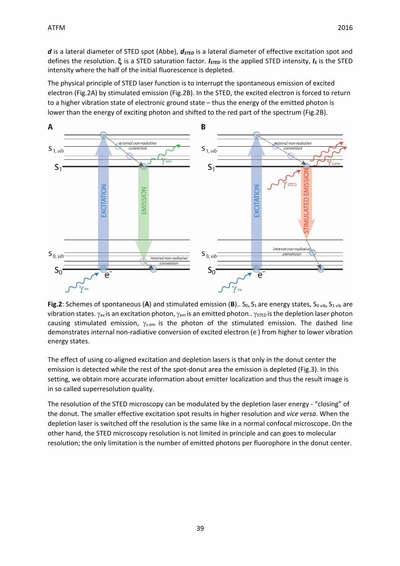
The physical principle of STED laser function is to interrupt the spontaneous emission of excited

electron (Fig.2A) by stimulated emission (Fig.2B). In the STED, the excited electron is forced to return

to a higher vibration state of electronic ground state – thus the energy of the emitted photon is

lower than the energy of exciting photon and shifted to the red part of the spectrum (Fig.2B).

Fig.2: Schemes of spontaneous (A) and stimulated emission (B).. S0, S1 are energy states, S0 vib, S1 vib are

vibration states. ex is an excitation photon, em is an emitted photon.. STED is the depletion laser photon

causing stimulated emission, s.em is the photon of the stimulated emission. The dashed line demonstrates internal non-radiative conversion of excited electron (e-) from higher to lower vibration energy states.

The effect of using co-aligned excitation and depletion lasers is that only in the donut center the

emission is detected while the rest of the spot-donut area the emission is depleted (Fig.3). In this

setting, we obtain more accurate information about emitter localization and thus the result image is

in so called superresolution quality.

The resolution of the STED microscopy can be modulated by the depletion laser energy - “closing” of

the donut. The smaller effective excitation spot results in higher resolution and vice versa. When the

depletion laser is switched off the resolution is the same like in a normal confocal microscope. On the

other hand, the STED microscopy resolution is not limited in principle and can goes to molecular

resolution; the only limitation is the number of emitted photons per fluorophore in the donut center.

ATFM 2016

40

Fig.3: The controlling of excitation spot area allows to precisely determine the fluorophore localization. A – a situation with normal confocal laser spot; B – STED donut co-aligned lasers spot when only fluorophores in the center emit photons; C – the much closed STED donut achieves the molecular resolution.

In reality, the emission depletion in the donut area is not absolute and a STED laser causes also the

anti-Stokes emission when the energy of the emitted photon is higher than the STED laser photon

energy (Fig.4).

The anti-Stokes effect is higher when the excitation spectrum of the fluorophore is closer to the STED

laser line. When the gap between the excitation spectrum of the fluorophore and STED laser line is

longer, the anti-Stokes emission is minimal. On the other hand, for the STED is necessary to overlap

the emission spectrum with the STED laser line otherwise the emission depletion does not work. The

selection of the proper fluorophore is crucial - we can reduce the anti-Stokes to minimum and scarify

the STED and the resolution or take one with high overlap between STED laser line and the

fluorophore emission spectrum and acquire high anti-Stokes emission and therefore totally blurred

image. The fluorophores selection must be balanced with the STED system configuration.

ATFM 2016

41

Fig.4: The illustration of anti-Stokes emission. The energy of the emitted photons are higher than the energy of the excitation. The electron in higher vibration state S0, vib is excited and internal non-radiative conversion is to the higher S1, vib states. Then, the anti-Stokes emission is possible.

Time gating improves the STED microscopy by increasing the resolution and also filtering out

significant part of anti-Stokes emission. In confocal microscopy it can be used for filtering unwanted

reflections. The essential equipment for time gating is a combination of pulse excitation laser and

suitable detector (e.g. GaAsP hybrid detector) which allows to acquire the signal from the

fluorophore in defined time interval after the excitation laser pulse (Fig.5).

Fig.5: A - The schematic illustration of a time gating setup; two pulses. The emission decay after the excitation laser pulse corresponds with the fluorophore lifetime. The anti-Stokes emission caused by continuous cwSTED laser is constant and excitation laser pulse independent. Tg is the time gap after the excitation pulse where the signal is not acquired. B - The effective excitation PSF diameter and its dependence on Tg value.

There are two important aspects for time gating setup. First, the decay of the emission fluorescence intensity has an exponential character while anti-Stokes emission caused by continuous STED laser is constant. It allows to close the time gating interval effectively to

ATFM 2016

42

acquire proportionally much more fluorescence emission signal compared to anti-Stokes signal (Fig.5A). Second, the improvement of the resolution due to time gating is based on changing the fluorophore lifetime within the center of the STED donut when the lifetime increases towards the center. Therefore, by the Tg increasing decreases emission PSF diameter and thus the resolution increases (Fig.5B). These two aspects depends on individual fluorophore and also chemical environment (e.g. used mounting solution) which both influence the emission lifetime (see Tab1) and thus must be balanced for each individual specimen.

Fluorophore Lifetime [ns] Solvent Excitation max

[nm] Emission max [nm]

ATTO 565 3.4 Water 561 585

Acridine Orange 2.0 PB pH 7.8 500 530

Acridine Yellow 470 550

Alexa Fluor 488 4.1 PB pH 7.4 494 519

Alexa Fluor 532 530 555

Alexa Fluor 546 4.0 PB pH 7.4 554 570

Alexa Fluor 633 3.2 Water 621 639

Alexa Fluor 647 1.0 Water 651 672

Alexa Fluor 680 1.2 PB pH 7.5 682 707

CY3B 2.8 PBS 558 572

CY3 0.3 PBS 548 562

CY3.5 0.5 PBS 581 596

Tab1: fluorescence emission lifetime of several common fluorophores.

ATFM 2016

43

02 STED – PRACTICAL PART

02.1 Equipment

Leica TCS SP8 STED 3X Inverted microscope DMI6000 AFC Bino with laser scanning confocal head Leica TCS SP8, motorized microscope stage with Super Z-galvo scanning insert for fast and precise Z movement, HW autofocus control, transmitted light equipment including transmitted light PMT, differential interference contrast available for all objectives. Confocal head is equipped with two fluorescence PMT detectors and one highly sensitive HyD detector with time resolved gating function. System is equipped with STED 3X module and 660 nm depletion laser and enables super-resolution imaging by stimulated depletion of emission (up to 50 nm lateral, 130nm axial resolution). Illumination: EL6000, Hg arc lamp, 120W Excitation lasers: Pulsed White Lite Laser (WLL2) 470 nm-640 nm with 1nm step, 8 parallel laser lines, 1.5 mW per each. Laser excitation and intensity is controlled by combination of AOTF. Continuous 405 nm DMOD Flexible laser with 50 mW output power. Depletion laser: 660 nm CW STED depletion laser, output power >1.5 W Objectives: HC PL APO 10x/0.40 CS HC PL APO 20x/0.75 CS IMM CORR CS2 STED White Objective CS 100x/1.40 OIL Fluorescence filtercubes / filterwheels: DAPI (A) (Ex:340-380, Em:LP425) FITC (I3) (Ex:450-490, Em:LP515) RHOD (N2.1) (Ex:515-560, Em:LP590) Cy5 (Y5 ET) (Ex:620/60, Em:700/75) Confocal scanning head: Confocal laser scanning head: Leica TCS SP8. Laser excitation switched and intensity regulated by acousto-optical tunable filter (AOTF). Conventional FOV SP8 scanner, maximal resolution 8192x8192px, speed 1-1800 Hz (7fps@512x512 px), hardware zoom 0.75x-48x, spectraly tunable detection, 2x PMT detectors (400-800nm), 1X HyD detector (400 – 720 nm) with time-gating function (0-12 ns with 0.1 ns step), 1x TLD detector for transmitted light. STED module: STED 3X with 3D STED function allows adjustment of xy and z resolution; maximal lateral resolution 50 nm, maximal axial resolution 130 nm.

Software: LAS X 64bit package with LAS AF SP8 Dye Finder, 3D visualization, deconvolution and colocalization module Software for STED deconvolution: Huygens professional, SVI. Instructor: Ivan Novotný, PhD, (Kateřina Rohlenová, MSc)

02.2 Aims

Using the STED microscopy technique, acquire images in superresolution; in situ specimens.

Compare several STED microscope settings, using the time gating and compare images resolution

ATFM 2016

44

with confocal microscope images. Measure subcellular structures diameter and estimate the

resolution. Using the deconvolution for raw 3D STED images, find the optimal raw image quality for

the deconvolution; evaluate the deconvolution quality.

02.2 Example of the Sample preparation for STED microscopy

1. Cell cultivation: Adherent cells were grown minimally 24h on high performance coverslip (rectangle,

18 mm in diameter, 170±5µm thickness) in appropriate media/additives; 70% confluence.

2. Cells fixation: Discard medium 3x wash specimen: 1xPBS buffer, RT

Load 4% PFA in PIPES buffer, 15 min, RT Discard PFA 3x wash specimen: 1xPBS buffer, RT 3. Permeabilization:

Discard PBS Add 0.2% TRITON solution in PBS, 5 min, RT 3x wash cells: 1xPBS buffer, RT 1x wash in dH2O Transfer cover glasses onto the 1xPBS buffer drops (250 µm) on the parafilm layer stuck to the bench desk (cells down). From now, all procedure proceeds on drops.

4. Blocking:

5% NGS (normal goat serum), 100 µm per coverslip, 10 min, RT 1x wash cells: 1xPBS buffer, RT

5. Immunostaining:

Incubate samples on the primary antibody solution, 50 µl per coverslip, 60 min, RT (for

the ATFM course were used mouse anti-Tubulin01 or rat anti-Nup or rabbit anti-Lamin or their combinations) 3x wash cells: 1xPBS buffer, 2 min per wash, RT Incubate samples on the secondary antibody solution, 50 µl per coverslip, 60 min, RT (for the ATFM course were used Goat anti-Mouse/Rabbit or Rat IgG (H+L) Secondary Antibody, Alexa Fluor® 555 conjugate or combination of 568 and 514; For the Alexa Fluor® we recommend the dilution 1:300) 3x wash cells: 1xPBS buffer, 2 min per wash, RT

6. Mounting: Wash properly coverslip with water - salts removing Dry glasses on the bench (cells up, e.g. 20 min, RT)

Mount cover glasses to the slides with mounting medium (5 µl per 18 mm rectangle cover glass (for the superresolution techniques is highly recommended to use non-hardening mounting media; in

ATFM 2016

45

combination with Alexa Fluor® fluorophores we routinely use 90% Glycerol mounting medium with 5% n-propylgalate as an anti-fade additive)

02.3 Settings of the experiment

- Tune the STED laser intensity (depends on fluorophore properties)

- Define the time gating interval

- Set a proper sampling (pixel size) for STED image - Do the confocal and STED image both with the STED sampling; compare - Measure intracellular structures

- Do the STED deconvolution: estimate the proper Signal to noise ratio (SNR), do the

deconvolution - Evaluate the deconvolved image, compare the contrast of the deconvolved image with the raw

one

02.4 Literature & recommended web sources

Buckers, J., D. Wildanger, G. Vicidomini, L. Kastrup and S. W. Hell (2011). "Simultaneous multi-lifetime multi-color STED imaging for colocalization analyses." Optics Express 19(4): 3130-3143. Hernandez, I. C., C. Peres, F. C. Zanacchi, M. d'Amora, S. Christodoulou, P. Bianchini, A. Diaspro and G. Vicidomini (2014). "A new filtering technique for removing anti-Stokes emission background in gated CW-STED microscopy." Journal of Biophotonics 7(6): 376-380. Javad N. Farahani, M. J. S. a. L. A. B. (2010). Stimulated Emission Depletion (STED) Microscopy: from Theory to Practice. Microscopy: Science, Technology, Applications and Education, FORMATEX ,C/ Zurbarán 1, 2º - Oficina 1, 06002 Badajoz Spain, 2: 1539-1547. Vicidomini, G., I. C. Hernandez, P. Bianchini and A. Diaspro (2013). "STED Microscopy with Time-Gated Detection: Benefits and Limitations." Biophysical Journal 104(2): 667a-668a. Vicidomini, G., I. C. Hernandez, M. d'Amora, F. C. Zanacchi, P. Bianchini and A. Diaspro (2014). "Gated CW-STED microscopy: A versatile tool for biological nanometer scale investigation." Methods 66(2): 124-130. Vicidomini, G., G. Moneron, K. Y. Han, V. Westphal, H. Ta, M. Reuss, J. Engelhardt, C. Eggeling and S. W. Hell (2011). "Sharper low-power STED nanoscopy by time gating." Nature Methods 8(7): 571-U575. Vicidomini, G., A. Schonle, H. S. Ta, K. Y. Han, G. Moneron, C. Eggeling and S. W. Hell (2013). "STED Nanoscopy with Time-Gated Detection: Theoretical and Experimental Aspects." Plos One 8(1).

ATFM 2016

46

Web sources (downloaded: 20151112)

https://en.wikipedia.org/wiki/Stokes_shift

https://en.wikipedia.org/wiki/STED_microscopy

https://en.wikipedia.org/wiki/Jablonski_diagram

http://www.leica-microsystems.com/science-lab/huygens-sted-deconvolution-increases-signal-to-

noise-and-image-resolution-towards-22-nm/

http://www.leica-microsystems.com/science-lab/gated-sted-microscopy-with-cw-sted-lasers/

__________________________________________________________________________________

Contact us:

Course Coordinator: Ivan Novotny, PhD Light Microscopy Core Facility Institute of Molecular Genetics AS CR Videnska 1083 14220 Praha 4 Czech Republic Phone: +420 296 44 3192 Fax: +420 224 310 955 E-mail: ivan.novotny@img.cas.cz

Administration: Lenka Pišlová Microscopy Centre Institute of Molecular Genetics of the ASCR Videnska 1083 142 20 Prague 4 Czech Republic Phone: +420 241 062 289 Fax: +420 241 062 289 lenka.pislova@img.cas.cz