asynchronous online testing of multiple hypotheses
TRANSCRIPT

Journal of Machine Learning Research 22 (2021) 1-39 Submitted 11/19; Revised 1/21; Published 1/21
Asynchronous Online Testing of Multiple Hypotheses
Tijana Zrnic [email protected]
Department of Electrical Engineering and Computer SciencesUniversity of California, BerkeleyBerkeley, CA 94720, USA
Aaditya Ramdas [email protected]
Department of Statistics and Data ScienceCarnegie Mellon UniversityPittsburgh, PA 15232, USA
Michael I. Jordan [email protected]
Department of Electrical Engineering and Computer SciencesDepartment of StatisticsUniversity of California, BerkeleyBerkeley, CA 94720, USA
Editor: Gabor Lugosi
AbstractWe consider the problem of asynchronous online testing, aimed at providing control of the false discovery rate(FDR) during a continual stream of data collection and testing, where each test may be a sequential test thatcan start and stop at arbitrary times. This setting increasingly characterizes real-world applications in scienceand industry, where teams of researchers across large organizations may conduct tests of hypotheses in adecentralized manner. The overlap in time and space also tends to induce dependencies among test statistics,a challenge for classical methodology, which either assumes (overly optimistically) independence or (overlypessimistically) arbitrary dependence between test statistics. We present a general framework that addressesboth of these issues via a unified computational abstraction that we refer to as “conflict sets.” We show howthis framework yields algorithms with formal FDR guarantees under a more intermediate, local notion ofdependence. We illustrate our algorithms in simulations by comparing to existing algorithms for online FDRcontrol.Keywords: FDR control, false discovery rate, sequential hypothesis testing, sequential experimentation,p-values
1. Introduction
As applications of machine learning expand in scope beyond the classical setting of a single decision-makerand a single dataset, the decision-making side of the field has become increasingly important. Unfortunately,research on the decision-making side of the field has lagged relative to the pattern-recognition side, oftenfocusing only on the validity of single decisions. Arguably, however, deployed machine learning modelswitness large collections of decisions, typically occurring in an extended asynchronous stream. In suchsettings, it is essential to consider error rates over sets of decisions, and not merely over single decisions.
Although it is not a focus of research in machine learning, multiple decision-making has been promi-nent during the past two decades in statistics, in the wake of seminal research by Benjamini and Hochberg(1995) on false discovery rate (FDR) control in multiple testing. That literature has, however, principallyfocused on batch data analysis and relatively small-scale problems. Modern applications in domains such asmedicine, commerce, finance, and transportation are increasingly of planetary scale, with statistical analy-sis and decision-making tools being used to evaluate hundreds or thousands of related hypotheses in smallwindows of time (see, e.g., Tang et al., 2010; Xu et al., 2015). These testing processes are often sequential,
c©2021 Tijana Zrnic, Aaditya Ramdas, and Michael I. Jordan.
License: CC-BY 4.0, see https://creativecommons.org/licenses/by/4.0/. Attribution requirements are provided athttp://jmlr.org/papers/v22/19-910.html.

ZRNIC, RAMDAS, AND JORDAN
conducted in the context of a continuing stream of data analysis. The sequentiality is at two levels—eachindividual test is often a sequential procedure, terminating at a random time when a stopping criterion issatisfied, and also the overall set of tests is carried out sequentially, with possible overlap in time. In thissetting—which we refer to as asynchronous online testing—the goal is to control a criterion such as the FDRnot merely at the end of a batch of tests, but at any moment in time, and to do so while recognizing that thedecision for a given test must generally be made while other tests are ongoing.
A recent literature on “online FDR control” has responded to one aspect of this problem, namely theproblem of providing FDR control during a sequence of tests, and not merely at the end, by adaptively settingthe test levels for the tests (Foster and Stine, 2008; Javanmard and Montanari, 2018; Ramdas et al., 2017,2018). These methods are synchronous, meaning that each test can only start when the previous test hasfinished. Our goal is to consider the more realistic setting in which each test is itself a sequential processand where tests can overlap in time. This is done in real applications to gain time efficiency, and becauseof the difficulties of coordination in a large-scale, decentralized setting. To illustrate this point, Figure 1compares the testing of five hypotheses within an asychronous setting and a synchronous setting. In theasynchronous setting, the test level αt used to test hypothesis Ht is allowed to depend only on the outcomesof the previously completed tests—for example, α3 can depend on the outcome of H1, however not on theoutcome of H2. In the synchronous setting, on the other hand, the test level αt can depend on all previouslystarted (hence also completed) tests. To account for the uncertainty about the tests in progress, the test levelsassigned by asynchronous online procedures must be more conservative. Thus, there is a tradeoff—althoughasynchronous procedures take less time to perform a given number of tests they are necessarily less powerfulthan their synchronous counterparts. The management of this tradeoff involves consideration of the overallpower achieved per unit of real time, and consideration of the complexity of the coordination required in thesynchronous setting.
Another limitation of existing work on online multiple testing is that the dependence assumptions on thetested sequence of test statistics, under which the formal false discovery rate guarantees hold, are usually atone of two extremes—they are either assumed to be independent, or arbitrarily dependent. From a practicalperspective, independence seems overly optimistic as new tests may use previously collected data to formulatehypotheses, or to form a prior, or as evidence while testing. On the other hand, arbitrary dependence is likelytoo pessimistic, as older data and test outcomes with time become “stale,” and no longer have direct influenceon newly created tests. We see that a reconsideration of dependence is natural in the setting of online FDRcontrol, and is particularly natural in the asynchronous setting, given that tests that are being conductedconcurrently are often likely to be dependent, since they may use the same or highly correlated data duringtheir overlap.
We therefore define and study a notion of local dependence, and place it within the context of asyn-chronous multiple testing. Working with p-values for simplicity, and letting Pt denote the t-th tested p-value,we say that a sequence of p-values {Pt} satisfies local dependence if the following condition holds:
for all t > 0, there exists Lt ∈ N such that Pt ⊥ Pt−Lt−1, Pt−Lt−2, . . . , P1, (1)
where {Lt} is a fixed sequence of parameters which we will refer to as “lags.” Clearly, when Lt = 0 for all t,we obtain the independent setting, and when Lt = t, we recover the arbitrarily dependent setting. If Lt ≡ Lfor all t, condition (1) captures a lagged dependence of order L.
To further emphasize the natural connection between asynchrony and local dependence, consider thesimple setting in Figure 2. This diagram captures the setting in which a research team is collecting data overtime, and decides to run multiple tests in a relatively short time interval. For example, such a situation mightarise when testing multiple treatments against a common control (Robertson and Wason, 2018), or in large-scale A/B testing by internet companies (Xu et al., 2015). Since there is overlap in the data these tests useto compute their test statistics, the corresponding p-values could be arbitrarily dependent. In general severaltests might share data with the first test. Thus the p-values are locally dependent, with the lag parameter beingequal to the number of consecutive tests that share data.
In this work, we reinforce this connection between asynchronous online testing and dependence by devel-oping a general abstract framework in which, from an algorithmic point of view, these two issues are treated
2

ASYNCHRONOUS ONLINE TESTING OF MULTIPLE HYPOTHESES
Figure 1: Testing five hypotheses synchronously (top) and asynchronously (bottom). In both cases, the testlevels αt depend on the outcomes of previously completed tests, which in the synchronous case includes allpreviously started tests. At the start time of experiment t, Wt−1 is used to denote the remaining “wealth”for making false discoveries. At the end of experiment t, a p-value Pt and its corresponding decision Rt : =1 {Pt ≤ αt} are known, which is used to adjust the available wealth at the start time of the next new test.
Figure 2: Example of p-values within a short interval computed on overlapping data. They exhibit localdependence; for example, P3 and P4 are independent of P1.
with a single formal structure. We do so by associating with each test a conflict set, which consists of othertests that have a potentially adversarial relationship with the test in question. Within this framework, we de-velop algorithms with provable guarantees on the rate of false discoveries. The core idea is to enforce a notionof pessimism with regard to the conflict set—when computing a new test level, the algorithm “hallucinates”the worst-case outcomes of the conflicting tests.
We derive procedures that handle conflict sets as strict generalizations of current state-of-the-art onlineFDR procedures; indeed, when there are no conflicts, for example when there is no asynchrony and when the
3

ZRNIC, RAMDAS, AND JORDAN
p-values are independent, our solutions recover LORD (Javanmard and Montanari, 2018), LOND (Javanmardand Montanari, 2015), and SAFFRON (Ramdas et al., 2018), the latter of which recovers alpha-investing(Foster and Stine, 2008) as a special case for a particular choice of parameters. On the other hand, if theconflict sets are as large as possible—for example, if the parameter Lt or the number of tests run in paralleltend to infinity—our algorithms behave like alpha-spending,1 which was designed to control a more stringentcriterion called the family-wise error rate (FWER), under any dependence structure. Independently, we alsoprove that the original LOND procedure controls the FDR even under positive dependence (PRDS), the firstonline procedure to provably have this guarantee under the PRDS condition that is popular in the offline FDRliterature (Benjamini and Yekutieli, 2001; Ramdas et al., 2019).
Organization. The rest of this paper is organized as follows. After a presentation of the general problemformulation and related work, Section 2 presents the key notion of conflict sets. We present two generalprocedures based on conflict sets, deferring their formal FDR guarantees to Section 6. In Section 3, we couchasynchronous testing in terms of conflict sets. In a similar fashion, in Section 4, we describe synchronoustesting of locally dependent p-values using conflict sets, and present procedures having FDR guaranteeswithin this environment. Section 5 then combines the ideas of local dependence and asynchronous testing intoan overall framework designed for testing asynchronous batches of dependent p-values. Section 6 providesadditional, stronger guarantees of the presented algorithms, which hold under more stringent assumptions onthe p-value sequence. In Section 7 we present simulations designed to explore our methods, comparing themto existing procedures that handle dependent p-values. Finally, we conclude the paper with a short discussionin Section 8. All proofs are deferred to the Appendix.
1.1 Technical preliminaries
We briefly overview the technical background upon which our work builds. Recall that the false discoveryrate (FDR) (Benjamini and Hochberg, 1995) is defined as follows:
FDR ≡ E [FDP] = E[|H0 ∩R||R| ∨ 1
],
where H0 is the unknown set of true null hypotheses and R is the set of hypotheses rejected by some proce-dure. Formally we haveH0 = {i : Hi is true}, R = {i : Hi is rejected}. The random ratio appearing insidethe expectation is called the false discovery proportion (FDP). It is also of theoretical and practical interest tostudy a related metric called the modified false discovery rate (mFDR):
mFDR ≡E[|H0 ∩R|
]E [|R| ∨ 1]
.
Foster and Stine (2008) show that in the long run the mFDR behaves similarly to the FDR in an onlineenvironment. Similarly, Genovese and Wasserman (2002) prove that the mFDR and FDR achieved by thecelebrated Benjamini-Hochberg procedure (Benjamini and Hochberg, 1995) become equivalent as the num-ber of hypotheses tends to infinity. In this work, we mainly focus on the control of mFDR, as we can providesimple proofs under less restrictive assumptions. Importantly, in the Appendix we provide a side-by-sidecomparison of the mFDR and FDR for all of the experiments in this paper; as we show there, the plots formFDR and FDR are visually indistinguishable when the number of non-nulls is non-negligible, and mFDRdominates the FDR when non-nulls are sparse. Thus, our experiments suggest that mFDR control suffices forFDR control as well.
In addition, we point out one advantage of mFDR over FDR which is especially relevant in the onlinecontext. Suppose that different sequences of hypotheses are tested with different algorithms controlling themFDR. Then, one can retroactively group the set of discoveries resulting from these different algorithms,
1. Alpha-spending is a generalization of the Bonferroni correction in which the assigned test levels do not have to be equal. In otherwords, the Bonferroni correction suggests testing n hypotheses under level α/n, while alpha-spending merely requires
∑ni=1 αi ≤
α, where αi is the test level for the i-th hypothesis.
4

ASYNCHRONOUS ONLINE TESTING OF MULTIPLE HYPOTHESES
all the while knowing that the mFDR is still controlled. If the original sets of discoveries come with FDRguarantees only, one cannot argue FDR control over the overall batch of discoveries. This decentralizedtesting of different sequences using different algorithms is particularly aligned with the online FDR setup,where not all hypotheses are known in advance. In fact, this “online” property of the mFDR was recognizedeven within offline FDR control (van den Oord, 2008).
To simplify our presentation, we will often suppress the distinction, referring to both of these metrics as“FDR.”
In online FDR control, the set of rejections possibly changes at each time step, implying changes inmFDR and FDR. Therefore, in online settings, we have to considerR(t), which is the set of rejections up totime t, and the naturally implied mFDR(t) and FDR(t). We will also use the symbol V(t) : = R(t) ∩ H0 todenote the set of false rejections made up to time t. The main objective of online FDR algorithms is to ensuremFDR(t) ≤ α or FDR(t) ≤ α, for a chosen level α and for all times t.
Many of the online FDR algorithms that have been proposed to date in the literature are special cases of thegeneralized alpha-investing (GAI) framework (Aharoni and Rosset, 2014). The initial interpretation of thesealgorithms, as put forward by Foster and Stine (2008), relied on a notion of dynamically changing “alpha-wealth.” Ramdas et al. (2017, 2018) subsequently presented an alternative perspective on GAI algorithms.In this view, GAI algorithms are viewed as keeping track of an empirical estimate of the true false discoveryproportion, denoted FDP(t), and they assign test levels αt in a way that ensures FDP(t) ≤ α for all timesteps t, where α is the pre-specified FDR level. In the earlier paper (Ramdas et al., 2017), they show thatsuch control of FDP estimates also yields FDR control. This perspective—which is equivalent to the earlier,wealth characterization of GAI algorithms—will provide the mathematical framework upon which we buildin this paper.
Finally, we recap the typical assumptions made for null p-values in the FDR literature. If a hypothesis Hi
is truly null, then the corresponding p-value Pi is stochastically larger than the uniform distribution (“super-uniformly distributed,” or “super-uniform” for short), meaning that:
If the null hypothesis Hi is true, then Pr{Pi ≤ u} ≤ u for all u ∈ [0, 1].
This condition is sometimes generalized to the online FDR setting by incorporating a filtrationF i−1, resultingin the following assumption:
If the null hypothesis Hi is true, then Pr{Pi ≤ u
∣∣ F i−1} ≤ u for all u ∈ [0, 1], (2)
Here, F i captures all relevant information about the first i tests. As we discuss in later sections, however,this condition can be overly stringent when there are interactions between p-values, and we will accordinglyintroduce weaker super-uniformity assumptions.
1.2 Problem formulation and contribution
We now give a formal introduction to the problem setting, at the same time introducing the necessary notationfor the sections to follow.
At time step t ∈ N, the test of hypothesisHt begins, and the p-value resulting from this test is denoted Pt.In contradistinction to the standard online FDR paradigm, Pt is not required to be known at time t; indeed,this test is not fully performed at time t, but is only initiated at time t. The decision time for Ht is denotedEt; this is the time of possible rejection. Fully synchronous testing is thus an instance of this setting in whichEt = t, as assumed in classical online FDR work. In general, however, Et 6= t. Note also that, unlike in theclassical online FDR problem, the set of rejections R(t) and false rejections V(t) at time t now consider notall {Pi : i ≤ t}, but only {Pi : Ei ≤ t}:
R(t) = {i ∈ [t] : Ei ≤ t,Hi is rejected}, V(t) = R(t) ∩H0.
In addition, to capture the desideratum of statistical validity in the face of data reuse, we allow the possibilityof the p-values not being completely independent; in particular, we allow local dependence. Here, we envi-sion Pt having arbitrary, possibly adversarial dependence on Pt−1, . . . , Pt−Lt
, while the dependence between
5

ZRNIC, RAMDAS, AND JORDAN
Pt and Pj , j < t−Lt is limited. For simplicity the reader can assume Pt ⊥ Pt−Lt−1, Pt−Lt−2, . . . , P1, how-ever in later sections we will discuss some restricted forms of dependence between Pt and Pj , for j < t−Lt,handled by our results.
We treat Et as fixed but unknown before time Et itself. While the p-value and the duration of a testcould indeed be dependent random quantities—for example, when the duration is a reasonably good proxyfor sample size—here Et is not the absolute duration on a meaningful time scale, but it merely captures howmany tests have started before the decision for the t-th test. Thus, treating Et as fixed roughly correspondsto asserting independence between Pt and the number of newly created tests before test t finishes. As weenvision a highly decentralized setting with little between-test coordination, we deem this assumption reason-able. We do, however, acknowledge the possibility of a more coordinated setting with Pt and Et randomlycoupled, and this is an important avenue for future work.
Under the setup described above, the goal is to produce test levels αt dynamically at the beginning ofthe t-th test, such that, despite arbitrary local dependence and regardless of the decision times Et, the falsediscovery rate is controlled at any given moment under a pre-specified level α. In this work, we provideprocedures which achieve this goal, both at all fixed times t ∈ N, as well as adaptively chosen stoppingtimes.
It is important to remark that, even under independence of p-values, we cannot simply ignore the asyn-chronous aspects of the problem and naively apply an existing online FDR algorithm. We discuss two suchplausible but naive applications of online methodology, and discuss why they are invalid.
One natural adjustment could be to apply an online FDR algorithm whenever each test finishes (that is,whichever test is the t-th one to finish, test it at level αt). This scheme would only assign αt to a test atthe end of that test, which is unrealistic because sequential hypothesis tests—parametric tests such as Wald’ssequential probability ratio test (SPRT), and nonparametric tests as well (Balsubramani and Ramdas, 2016)—typically require specification of the target type I error level in advance because it is an important componentof their stopping rule. For examples of sequential tests in clinical trials, see, e.g., (Bartroff et al., 2012;Bartroff and Lai, 2008; Bartroff and Song, 2014). The same constraint holds for more recent, multi-armedbandit approaches to A/B testing (Yang et al., 2017; Jamieson and Jain, 2018). Thus, we need to specify αt atthe start of test t. That said, there do exist tests which only require the test level at decision time. If all testsin the sequence are of the latter kind, existing online methodology is indeed sufficient; however, we find thisassumption too strong, especially given the popularity of bandit approaches in modern testing applications.
Alternatively, one could imagine computing αt at the start of test t by applying an online FDR algorithmto the completed tests only, and ignoring those that have not finished. From the theory perspective, thisclearly comes with no formal guarantee; for example, one could imagine starting N tests, and all N testsfinishing at once, after the N -th test has started. Given that there are no completed tests at the time of testlevel assignment, all tests would receive the same level, which would violate the FDR requirement under anynatural setting (we ignore trivial special cases such as all hypotheses being non-null). Somewhat less trivially,Figure 3 plots the FDR and mFDR achieved by this naive heuristic in a simulation setting from Section 7.When the proportion of non-null p-values is relatively small—as one would generally expect in practice—thisheuristic severely violates the FDR requirement.
1.3 Related work
There is a vast literature on sequential testing (see, e.g., Wald, 1945; Chernoff, 1959; Albert, 1961; Naghshvarand Javidi, 2013). We do not aim to contribute to that literature per se; rather, our goal is to consider multipletesting through a more realistic lens as an outer sequential process, one that acknowledges the existence ofinner sequential processes that are based on sequential testing.
Likewise, there is a large and growing literature on false discoveries in multiple testing, aimed at solvinga range of problems, often addressing issues of scientific reproducibility in research (Ioannidis, 2005). Herewe focus on work whose methods or objectives have the most overlap with ours. In particular, we focus onliterature on “online” methods in multiple testing, and compare and contrast those solutions to the ones wepropose.
6

ASYNCHRONOUS ONLINE TESTING OF MULTIPLE HYPOTHESES
0.0 0.1 0.2 0.3 0.4 0.5 0.6 0.7 0.8 0.9
π1
0.0
0.1
0.2
0.3
0.4
0.5
0.6
0.7
0.8
0.9
1.0
FD
R
naive LORD
0.0 0.1 0.2 0.3 0.4 0.5 0.6 0.7 0.8 0.9
π1
0.0
0.1
0.2
0.3
0.4
0.5
0.6
0.7
0.8
0.9
1.0
mF
DR
naive LORD
Figure 3: FDR and mFDR achieved by a naive application of the LORD algorithm with target FDR levelα = 0.05 (Javanmard and Montanari, 2018) in an asynchronous environment. We adopt the experimentalsetting from Section 7; we set the asynchrony parameter to p = 1/150, and the mean of observations underthe alternative to µc = 3. Here, π1 is the proportion of tested hypotheses which are non-null. Both FDR andmFDR are controlled only for π1 ≥ 0.4.
The most salient difference is that we address the general problem of asynchrony; when there is noasynchrony, meaning Et = t, our approach recovers a slew of existing methods, including work by Fosterand Stine (2008), Aharoni and Rosset (2014), Javanmard and Montanari (2015, 2018), Ramdas et al. (2017,2018).
Most previous work also differs from ours in that it assumes that condition (2) holds. This condition istoo strong for the notion of local dependence this paper considers; indeed, in Section 4 we present a simpletoy example in which this assumption fails. An exception is the work of Javanmard and Montanari (2015,2018), who discuss sufficient conditions for achieving FDR control under arbitrary dependence within thep-value sequence. However, these conditions essentially imply an alpha-spending-like correction for the testlevels, making their proposed procedure overly conservative. We elaborate on this argument and empiricallydemonstrate this observation in Section 7.
Robertson and Wason (2018) have investigated the performance of several online FDR algorithms empir-ically, including all of those listed above, when the p-value sequence is positively dependent. They do not,however, provide any formal guarantees for those procedures that have thus far been shown to work only un-der independence. We make partial progress to justifying their empirical observations by proving that LONDprovably controls FDR under positive dependence.
Recently, there has also been some work specifically motivated by controlling false discoveries in A/Btesting in the tech industry (Yang et al., 2017). However, their setup was again fully synchronous, and assumethat the observations are independent across all experiments, which are the two assumptions this paper deemstoo strong and circumvents.
The vast literature on adaptive data analysis (Dwork et al., 2015b,a; Bassily et al., 2016; Blum and Hardt,2015) focuses on an online setting where a distribution is adaptively queried for a chosen functional, and ateach step these queries are answered by making use of a single data set coming from that distribution. Thisline of work also has the goal of preventing false discovery, however by proving generalization bounds, ratherthan controlling the FDR in online multiple testing.
Ordered hypothesis testing considers tests for which additional prior information is available, and allowssorting null hypotheses from least to most promising (Li and Barber, 2017; Lei and Fithian, 2016; Lynchet al., 2017; G’Sell et al., 2016). In these papers, however, the word “sequential” or “ordered” does not referto online testing; these methods are set in an offline environment, requiring access to all p-values at once. Inour approach, we allow testing a possibly infinite number of hypotheses with no available knowledge of thefuture p-values.
7

ZRNIC, RAMDAS, AND JORDAN
2. Conflict sets: the unifying approachIn this section we describe a general, abstract formulation of multiple testing under asynchrony and depen-dence, which unifies the seemingly disparate solutions of this paper and provides the point of departure forderiving specific algorithms. We describe two such procedures, which we will refer to as LORD* and SAF-FRON*, that control mFDR within this framework.
LORD* and SAFFRON* build off the LORD (Javanmard and Montanari, 2018) and SAFFRON (Ramdaset al., 2018) algorithms. Like SAFFRON, SAFFRON* allows the user to choose a parameter λt ≥ αt, whichis the “candidacy threshold” at time t, meaning that, if Pt ≤ λt, then Pt is referred to as a candidate forrejection. We will discuss this extension introduced in the SAFFRON procedure further below; for now, wesimply note that it is an analog of the notion of “null-proportion adaptivity” in the offline multiple testingliterature. Indeed, Ramdas et al. (2018) argue that LORD can be seen as the online analog of the BH pro-cedure (Benjamini and Hochberg, 1995), while SAFFRON can be seen as the online analog of the adaptiveStorey-BH procedure (Storey, 2002; Storey et al., 2004).
Throughout we let Rt : = 1 {Pt ≤ αt} denote the indicator for rejection, and Ct : = 1 {Pt ≤ λt} denotethe indicator for candidacy.
We now define several filtrations, which capture the increasing information available to the experimenteras well as the FDR algorithm.
By Lt, we denote a filtration that captures all relevant information about the tests that started up to, andincluding, time t, for the LORD* procedure. Formally, Lt : = σ({R1, . . . , Rt, }). For SAFFRON*, we alsoincorporate candidates in the filtration: St : = σ({R1, C1, . . . , Rt, Ct}). Many of our arguments will applyto both algorithms; we accordingly use F t to indicate a generic filtration that can be either Lt or St.
With each test and its corresponding hypothesis, we associate a conflict set. For the test starting at stept, we denote this set X t; it consists of a (not necessarily strict) subset of {1, . . . , t − 1}. For example, X 5
could be {3, 4}. The reason why we refer to this set as conflicting for test t is because it contains the indicesof tests that interact with the t-th test in some unknown way. This could mean that, at time t, there is missinginformation about these tests, or that there potentially exists some arbitrary dependence between those testsand the upcoming one. More explicitly, we let
X t = {i ∈ [t− 1] : Ei ≥ t} ∪ {t− Lt, . . . , t− 1},
where Lt is the sequence of dependence lags. In words, X t consists of all tests that have not finished runningor are locally dependent with test t.
We require the conflict sets to be monotone: each index t has to be in a continuous “block” of conflictsets. More formally, if there exists j such that t ∈ X j , then t ∈ X i, for all i ∈ {t + 1, . . . , j}. Without anyconstraint on the sequence {Lt}, the conflict sets need not be monotone. Therefore, we translate the conditionof monotonicity of conflict sets into a constraint on the sequence {Lt} as: Lt+1 ≤ Lt + 1. Informally, this isjust a requirement that the “non-conflicting information” does not decrease with time. This will ensure thatthe test level αt and candidacy threshold λt have at least as much knowledge about prior tests as αt−1 andλt−1. Moreover, this requirement is indeed a natural one, and usual testing practices satisfy it; for example,this condition holds if dependent p-values come in disjoint blocks.
We define the last-conflict time of test t as τt : = max{j : t ∈ X j}. If test t never appears in a conflictset, we take τt = t.
Consider again the filtration F t. A subtlety we initially ignored is that the superscript t does not corre-spond to the physical quantity of time. In particular, different tests may run for different lengths of time andthe decision time for each test may even be random; therefore, Rt might be known before Rt−1. This moti-vates us to define a filtration as a counterpart ofF t whose increase at each step corresponds to the real increasein knowledge with time. We introduce F−X t
as the non-conflicting filtration; the sigma-algebra F−X t
con-tains information about the tests that started before time t which are not in the conflict set of test t. In partic-ular, L−X t
: = σ({Ri : i ≤ t− 1, i 6∈ X t}) for LORD*, S−X t
: = σ({Ri, Ci : i ≤ t− 1, i 6∈ X t}) for SAF-FRON*, and again we use F−X t
to generically denote either L−X t
or S−X t
. We have that F−X t ⊆ F t−1.Notice that we promised to make this set a filtration; if X t was an arbitrary set of indices, this would not in
8

ASYNCHRONOUS ONLINE TESTING OF MULTIPLE HYPOTHESES
general be satisfied. However, it is straightforward to verify that the monotonicity property of conflict setsensures that F−X t
indeed forms a filtration.We will design αt and λt to be F−X t
-measurable. This is essentially the idea of pessimism mentionedearlier—among all tests that finished before the t-th one starts, αt and λt have to ignore the ones conflictingwith test t in order to guard against unknown interactions that the conflicting tests have with the upcomingone.
Finally, we will generally require the following super-uniformity condition for null p-values:
If the null hypothesis Ht is true, then Pr{Pt ≤ u
∣∣∣ F−XEt}≤ u, for all u ∈ [0, 1]. (3)
This is a condition that requires validity of null p-values: given the knowledge one has before making adecision, if a hypothesis is truly null, it has to be well-behaved. However, unlike in classical online FDRwork, we do not have F−XEt
= F t−1. As we discuss further in later sections, assumption (3) will allowarbitrary local dependence, as well some limited, but nevertheless important, forms of dependence betweendistant p-values. Note that, if the distant p-values are independent—a setting we study in Section 4 andSection 5—this condition is automatically satisfied.
2.1 The LORD* algorithm
Following a recently proposed framework (Ramdas et al., 2017), we define LORD* and SAFFRON* asarbitrary update rules which control a certain estimate of the false discovery proportion under a pre-specifiedlevel α; the two algorithms differ in their choice of estimate. In Subsection 2.3, we introduce additionalanalysis tools which will justify the choice of these estimates.
LORD* is defined as any update rule for αt that ensures that the estimate
FDPLORD*(t) : =
∑j≤t αj
(∑j≤t,j 6∈X t Rj) ∨ 1
.
is at most α for all t ∈ N.Below we state two different versions of LORD*, using two different test level updates. Algorithm 1
generalizes the LORD++ procedure (Javanmard and Montanari, 2018; Ramdas et al., 2017), while Algorithm2 generalizes its predecessor, the LOND procedure (Javanmard and Montanari, 2015). These are not the onlyways of assigning αj that are consistent with the assumptions and satisfy the definition of LORD* in theircontrol of FDPLORD*, but they are our focus in the remainder of the paper. Other rules can be developed asextensions of the rules in the LORD paper (Javanmard and Montanari, 2018).
To state the algorithms in this paper, we will make use of the variable rk, which refers to the first timethat k rejections are non-conflicting, meaning that there exist k rejected hypotheses which are no longer inthe conflict set at that time. That is, we define rk as:2
rk : = min{i ∈ [t] :
i∑j=1
Rj1 {τj ≤ i} ≥ k}. (4)
Algorithm 1 The LORD++ algorithm under general conflict sets (a special case of LORD*)input: FDR level α, non-negative non-increasing sequence {γj}∞j=1 such that
∑j γj = 1, initial wealth W0 ≤ α
Set α1 = γ1W0
for t = 1, 2, . . . dostart t-th test with level αt
αt+1 = γt+1W0 + γt+1−r1 (α−W0) +(∑
j≥2 γt+1−rj
)α
end
2. Here, as well as in the rest of this paper, we define the minimum of an empty set to be −∞.
9

ZRNIC, RAMDAS, AND JORDAN
Algorithm 2 The LOND algorithm under general conflict sets (a special case of LORD*)input: FDR level α, non-negative non-increasing sequence {γj}∞j=1 such that
∑j γj = 1
Set α1 = γ1αfor t = 1, 2, . . . do
start t-th test with level αt
αt+1 = αγt+1
((∑t
j=1 1 {Pj ≤ αj , τj ≤ t}) ∨ 1)
end
It is a simple algebraic exercise to verify that the two update rules given for αt indeed guarantee thatFDPLORD*(t) ≤ α for all t ∈ N.
2.2 The SAFFRON* algorithm
In response to LORD and LOND’s FDP estimate, the SAFFRON method was derived after observing thatthe former might be overly conservative estimates of the FDP. Indeed, if the tested sequence contains asignificant fraction of non-nulls, and if the non-nulls yield strong signals for rejection, the realized FDP andthe estimated FDP might be very far apart. Motivated by this observation, SAFFRON was developed as theadaptive counterpart of LORD which keeps track of an empirical estimate of the null proportion, similar to theway in which Storey et al. (Storey, 2002; Storey et al., 2004) improved upon the BH procedure (Benjaminiand Hochberg, 1995). We thus propose the SAFFRON* algorithm to maintain control over the followingestimate:
FDPSAFFRON*(t) : =
∑j<t,j 6∈X t
αj
1−λj1 {Pj > λj}+
∑j∈{X t∪{t}}
αj
1−λj
(∑j≤t,j 6∈X t Rj) ∨ 1
.
Any update rule for αt and λt ensuring FDPSAFFRON*(t) ≤ α for all t ∈ N satisfies the definition of SAF-FRON*. Algorithm 3 and Algorithm 4 describe two particular instances of SAFFRON*, obtained for specificchoices of the sequence {λj}. We present an algorithmic specification of SAFFRON* for the constant se-quence {λj} ≡ λ in Algorithm 3. A different case of SAFFRON* is presented in Algorithm 4, where we usethe alpha-investing strategy λj = αj (Foster and Stine, 2008; Ramdas et al., 2018).
For the updates below, recall the definition of rk from equation (4).
Algorithm 3 The SAFFRON* algorithm for constant λ under general conflict setsinput: FDR level α, non-negative non-increasing sequence {γj}∞j=1 such that
∑j γj = 1, candidate threshold λ ∈ (0, 1), initial
wealth W0 ≤ αα1 = (1− λ)γ1W0
for t = 1, 2, . . . dostart t-th test with level αt
αt+1 = min{λ, (1− λ)
(W0γt+1−C0+
+ (α−W0)γt+1−r1−C1++∑
j≥2 αγt+1−rj−Cj+
)},
where Cj+ =∑t
i=rj+1 Ci1{i 6∈ X t
}end
Algorithm 4 The alpha-investing algorithm under general conflict sets (a special case of SAFFRON*)input: FDR level α, non-negative non-increasing sequence {γj}∞j=1 such that
∑j γj = 1, initial wealth W0 ≤ α
s1 = γ1W0
α1 = s1/(1 + s1)for t = 1, 2, . . . do
start t-th test with level αt
st+1 =W0γt+1−R0++ (α−W0)γt+1−r1−R1+
+∑
j≥2 αγt+1−rj−Rj+, where Rj+ =
∑ti=rj+1Ri1
{i 6∈ X t
}αt+1 = st+1/(1 + st+1),
end
10

ASYNCHRONOUS ONLINE TESTING OF MULTIPLE HYPOTHESES
2.3 Oracle estimate under conflict sets
Following Ramdas et al. (2018), we analyze LORD* and SAFFRON* through an oracle estimate of the falsediscovery proportion. This quantity serves as a good estimate of the true false discovery proportion, andcontrolling it under a pre-specified level guarantees that FDR is also controlled. Let the oracle estimate of theFDP be defined as:
FDP∗(t) : =
∑j≤t,j∈H0 αj
(∑Ej≤tRj) ∨ 1
,
where we recall that αj is required to be F−X j
-measurable, across all j. The following proposition givesformal justification for using FDP∗(t) as a proxy for the true FDP.
Proposition 1 Suppose that the null p-values are super-uniform conditional onF−XEt , meaning Pr{Pt ≤ u
∣∣∣ F−XEt}≤
u, for all u ∈ [0, 1] and t ∈ H0. Then, for all times t ∈ N, the condition FDP∗(t) ≤ α implies thatmFDR(t) ≤ α.
Note that Proposition 1 is technically true even if we only consider tests for which Ej ≤ t, j ∈ H0 inthe numerator of FDP∗(t). However, it is not clear how to achieve this without ensuring FDP∗(t) ≤ α. For
example, even if∑
Ej≤t,j∈H0 αj
(∑
Ej≤t Rj)∨1 ≤ α at time t, it is possible that in subsequent rounds all tests will finish
without any new rejections, thus increasing the FDP estimate. Therefore, we need to assign αj conservatively,such that this estimate is provably controlled underα, despite unknown future outcomes which might augmentthe FDP estimate.
The fact that αt is measurable with respect to F−X t
should give us pause. Even though we are onlyrequired to guarantee FDP∗(t) ≤ α, we cannot rely on the rejection indicators that push down the value ofFDP∗(t), if they are in the current conflict set. As a consequence, αt has to ensure FDP∗(t) ≤ α for theworst-case configuration of conflicting rejections; that is, when Rj = 0 for all j ∈ X t. This motivates us todefine the oracle estimate of the FDP under conflict sets:
FDP∗conf(t) : =
∑j≤t,j∈H0 αj
(∑
j≤t,j 6∈X t Rj) ∨ 1. (5)
Since this quantity is only more conservative than the oracle estimate, controlling it under α will preservethe guarantees given by Proposition 1. However, notice an unfortunate fact about both oracle estimates—theydepend on the unobservable set H0. This implies that not even FDP∗conf(t) can be controlled tightly. For thisreason, LORD* and SAFFRON* construct empirical estimates of FDP∗conf(t), such that the properties givenin Proposition 1 are retained. For LORD*, claiming mFDR control at fixed times boils down to a simpleobservation: for any chosen α, FDP∗conf(t) ≤ FDPLORD*(t) ≤ α, hence by Proposition 1 mFDR is controlled.SAFFRON* controls mFDR by virtue of ensuring that, on average, FDP∗conf(t) ≤ α. We make this argumentformal in Section 6.
3. Example 1: Asynchronous online FDR controlIn this section, we look at one instantiation of the conflict-set framework, which considers arbitrary asyn-chrony but limits possible dependencies between p-values. This immediately gives two procedures for asyn-chronous online testing as special cases of LORD* and SAFFRON*. From here forward we will refer to thesemethods as LORDasync and SAFFRONasync, respectively. In Section 6, we provide mFDR guarantees of theseprocedures in terms of the general conflict-set setting, as well as additional FDR guarantees for LORDasyncand SAFFRONasync under a strict independence assumption.
In this section, the only conflicting tests are those whose outcomes are unknown, since the allowed de-pendencies will be fairly restrictive. Therefore, the asynchronous conflict set at time t is:
X tasync = {i ∈ [t− 1] : Ei ≥ t},
11

ZRNIC, RAMDAS, AND JORDAN
which is observable at time t − 1. This simplified conflict set implies that the last-conflict time of test t is,naturally, τt = Et.
Denote byRt the set of rejections at time t, and similarly let Ct denote the set of candidates at time t:
Rt = {i ∈ [t] : Ei = t, Pi ≤ αi}, Ct = {i ∈ [t] : Ei = t, Pi ≤ λi}.
Therefore,R(t) = ∪ti=1Rt. With this, we can write the non-conflicting filtrationsL−X t
async and S−X t
async compactlyas:
L−Xt
async : = σ(R1, . . . ,Rt−1), S−Xt
async : = σ(R1, C1, . . . ,Rt−1, Ct−1).
Since the arguments for LORDasync and SAFFRONasync have significant overlap, for brevity we write F−X t
async
to refer to both L−X t
async and S−X t
async , where possible. Recall from Section 2 that αt is designed to be measurablewith respect to F−X t
async ; here this essentially means that it is computed as a function of the outcomes knownby time t. For SAFFRONasync, additionally λt is S−X t
async -measurable. More generally, for LORDasync, wecan choose αt = ft(R1, . . . ,Rt−1), for any deterministic function ft as long as the correct FDP estimateis controlled. The SAFFRONasync procedure also keeps track of encountered candidates, hence we can takeαt = gt(R1, C1, . . . ,Rt−1, Ct−1) and λt = ht(R1, C1, . . . ,Rt−1, Ct−1), for deterministic functions gt andht.
Our mFDR guarantees hold under a condition which we term asynchronous super-uniformity:
If the null hypothesis Ht is true, then Pr{Pt ≤ u
∣∣∣ F−XEt
async
}≤ u, for all u ∈ [0, 1]. (6)
This condition essentially shapes the allowed dependencies between p-values. It is immediately implied ifthe p-values are independent. However, it is strictly weaker. For example, it allows revisiting p-values whichwere previously not rejected. Suppose we have tested independent p-values thus far, and we failed to rejectHt, that is Pt > αt. If at a later time s > t we have a higher error budget αs > αt, we can, somewhatsurprisingly, test Ht using the same p-value Pt again at time s. This clearly violates independence of Pt andPs (as they are identical), however condition (6) is nevertheless satisfied. Indeed, for all u > αt:
Pr{Ps ≤ u
∣∣∣ F−XEs
async
}= Pr{Ps ≤ u | Ps > αt} ≤
u− αt1− αt
≤ u,
where the equality follows becausePs ⊥ F−XEs
async | 1 {Ps > αt}. On the other hand, if u ≤ αt, Pr{Ps ≤ u | Ps > αt} =0 ≤ u, and hence condition (6) follows.
The LORDasync and SAFFRONasync algorithms
We turn to an analysis of how the abstract LORD* and SAFFRON* procedures translate into our asyn-chronous testing scenario, for the particular choice of conflict set X tasync. They utilize all available informa-tion; the conflict set—the tests whose outcomes the algorithms ignore—consists only of the tests about whichwe temporarily lack information.
Plugging in the definition of X tasync, we obtain the following empirical estimate of the false discoveryproportion for LORDasync:
FDPLORDasync(t) =
∑j≤t αj
(∑j≤t 1 {Pj ≤ αj , Ej < t}) ∨ 1
.
For SAFFRONasync, we obtain the following estimate:
FDPSAFFRONasync(t) =
∑j≤t
αj
1−λj(1 {Pj > λj , Ej < t}+ 1 {Ej ≥ t})
(∑j≤t 1 {Pj ≤ αj , Ej < t}) ∨ 1
.
12

ASYNCHRONOUS ONLINE TESTING OF MULTIPLE HYPOTHESES
Consider the dynamics of these two algorithms, and how their pessimism comes into play. Whenevera test starts, they increase their FDP estimate, expecting that the resulting p-value will have no favorablecontribution. However, when the test in question ends, they readjust the FDP estimate if they see a positiveoutcome, namely a candidate and/or rejection. This shows that testing in parallel indeed has a cost—due topessimistic expectations about the tests in progress, the algorithms remain conservative when assigning a newtest level. For this reason, asynchronous testing should be used with caution, and the number of tests run inparallel should be monitored closely. Indeed, in the asymptotic limit where the number of parallel tests tendsto infinity, the algorithm behaves like alpha-spending; i.e., the sum of all assigned test levels converges to theerror budget α.
Substituting X t for X tasync in Algorithms 1-4 yields procedures for asynchronous online FDR control. Theexplicit statements of these algorithms, which correspond to asynchronous versions of LORD++, LOND,SAFFRON, and alpha-investing, are given in the Appendix.
4. Example 2: Online FDR control under local dependenceIn this section, we derive online FDR procedures that handle local dependencies. We begin with the fullysynchronous setting studied in classical online FDR literature, and turn to the asynchronous environment inthe next section.
A standard assumption in existing work on online FDR has been independence of p-values, a requirementthat is rarely justified in practice. Tests that cluster in time often use the same data, null hypotheses dependon the outcomes of recent tests, etc. On the other hand, arbitrary dependence between any two p-values inthe sequence is also arguably unreasonable—very old data used for testing in the past is usually considered“stale,” and hypotheses tested a long time ago may bear little relevance to current hypotheses. In light of this,we consider a notion of local dependence:
for all t > 0, there exists Lt ∈ N such that Pt ⊥ Pt−Lt−1, Pt−Lt−2, . . . , P1,
where {Lt} is a fixed sequence of parameters which we refer to as lags.Since we allow Pt to have arbitrary dependence on the previous Lt p-values, some of these dependencies
might be adversarial toward the statistician, and, with “peeking” into this adversarial set, the nulls might nolonger behave super-uniformly. Suppose we observe a sample X ∼ N(µ, 1), and wish to test two hypothesesusing this sample. Let the two hypotheses be H1 : µ < 0 and H2 : µ ≥ 0. If, for instance, R1 = 0, we knowthat P2 ≤ 1−α1 almost surely, implying that P2 is not super-uniform, given the information about past tests.On the other hand, if we were to ignore the outcome of the first test, P2 would indeed be super-uniform.
This observation motivates us to define the conflict set for testing under local dependence as:
X tdep : = {t− Lt, . . . , t− 1}.
The non-conflicting filtrations L−Xt
dep for LORDdep and S−Xt
dep for SAFFRONdep are respectively given by:
L−Xt
dep : = σ(R1, . . . , Rt−Lt−1), S−Xt
dep : = σ(R1, C1, . . . , Rt−Lt−1, Ct−Lt−1).
Since most formal arguments in this section apply to both procedures, we use F−Xt
dep to indicate that the
filtration in question could be both L−Xt
dep and S−Xt
dep .In contrast to asynchronous testing, the levels αt and λt under local dependence ignore some portion of
available information, specifically the outcomes of the last Lt tests. Notice the difference between these twosettings—in the asynchronous setting, pessimism guards against unknown outcomes, while here pessimismguards against known outcomes. Perhaps counterintuitively, this observation means that the pessimism ofLORDdep and SAFFRONdep actually guards against possible disadvantageous direct impact of the last Ltp-values on the upcoming one. In the Appendix we instantiate the test levels and candidacy thresholdsaccording to Algorithms 1-4, however more generally we allowαt = ft(R1, . . . , Rt−Lt−1) for LORDdep, andαt = gt(R1, C1, . . . , Rt−Lt−1, Ct−Lt−1) and λt = ht(R1, C1, . . . , Rt−Lt−1, Ct−Lt−1) for SAFFRONdep.
13

ZRNIC, RAMDAS, AND JORDAN
Consider some Pt which is from a null hypothesis. As previously emphasized, we cannot trust Pt tobehave like a true null, given that we already know its last Lt predecessors that have a direct impact on it.The appropriate super-uniformity condition satisfied by locally dependent p-values thus ignores these last Ltp-values and is of the following form:
If the null hypothesis Ht is true, then Pr{Pt ≤ u
∣∣∣ F−X t
dep
}≤ u, for all u ∈ [0, 1]. (7)
This will allow setting αt ∈ F−Xt
dep , while knowing Pr{Pt ≤ αt
∣∣∣ F−X t
dep
}≤ αt. Importantly, unlike in
the previous section where the appropriate super-uniformity condition implied dependence constraints on thep-values, condition (7) is immediately true by local dependence.
The LORDdep and SAFFRONdep algorithms
As in Section 3, we analyze the particular instances of LORD* and SAFFRON* that are obtained by takingthe conflict set of Section 2 to be X tdep = {t − Lt, . . . , t − 1}. Since this conflict set is deterministic,unlike X tasync, the estimate of the false discovery proportion that LORDdep and SAFFRONdep keep track of iscompletely determined Lt steps ahead, that is at time t− Lt − 1.
By definition of the general estimates and the conflict set in consideration, LORDdep controls the follow-ing quantity:
FDPLORDdep(t) =
∑j≤t αj
(∑j≤t,j 6∈{t−Lt,...,t−1}Rj) ∨ 1
.
The SAFFRONdep method, on the other hand, controls the estimate:
FDPSAFFRONdep(t) =
∑j<t−Lt
αj
1−λj1 {Pj > λj}+
∑tj=t−Lt
αj
1−λj
(∑j≤t,j 6∈{t−Lt,...,t−1}Rj) ∨ 1
.
In the case of running asynchronous tests, the algorithms were constructed as pessimistic; however, theyhad access to as much information as the statistician performing the tests. Here, that is not the case—LORDdepand SAFFRONdep choose to ignore the outcomes of completed tests as long as they are in the conflict set ofsubsequent tests. Only after the last-conflict time τi, positive outcomes are rewarded by readjusting theFDP estimate. On the other hand, the statistician’s perspective is different—as soon as round t is over, thestatistician knows the outcome of the t-th test. Just like testing in parallel, testing locally dependent p-valuescomes at a cost—if the lags are large, the algorithm keeps increasing the FDP estimate, assigning ever smallertest levels, waiting for rewards from tests performed a long time ago. In the extreme case of Lt = t, the testlevels steadily decrease so that their sum converges to α, regardless of the fact that discoveries have possiblybeen made.
Explicit setting-specific algorithms, obtained by substituting X t for X tdep in Algorithms 1-4, resulting inLORD++, LOND, SAFFRON, and alpha-investing under local dependence, are given in the Appendix.
5. Example 3: Controlling FDR in asynchronous mini-batch testingHere we merge the ideas of the previous two sections, bringing together asynchronous testing and localdependence of p-values. Although there are various ways one could think of in which these two conceptsintertwine, here we discuss a particularly simple and natural one.
Let a mini-batch represent a grouping of an arbitrary number of tests that are run asynchronously, whichresult in dependent p-values; for instance, these tests could be run on the same data. After a mini-batchof tests is fully executed, a new one can start, testing new hypotheses, independent of the previous batch,and doing so on fresh data. From the point of view of asynchrony, such a process could be thought of as acompromise between synchronous and asynchronous testing—batches are internally asynchronous, howeverthey are globally sequential and synchronous. If all batches are of size one, one recovers classical online
14

ASYNCHRONOUS ONLINE TESTING OF MULTIPLE HYPOTHESES
testing; if the batch-size tends to infinity, the usual notion of asynchronous testing is obtained. Figure 4depicts an example of a mini-batch testing process with three mini-batches.
Figure 4: Running three mini-batches of tests. The batches are run synchronously, while the tests that com-prise each of them are run asynchronously. We use Wt,j−1 to denote the remaining "wealth" for making falsediscoveries before starting the j-th test in the t-th batch.
We introduce notation that captures this setting. We will use two time indices; Pb,t denotes the p-valueresulting from the test that starts as the t-th one in the b-th batch, testing hypothesis Hb,t. We allow any twop-values in the same batch to have arbitrary dependence; however, we require any two p-values in differentbatches to be independent. This can be written compactly as:
Pb1,i ⊥ Pb2,j , for any b1, b2, i, j, such that b1 6= b2.
We will denote the size of the b-th batch as nb. Thus, the first batch results in P1,1, . . . , P1,n1 , thesecond one in P2,1, . . . , P2,n2 , etc. Analogously, the test levels and candidacy thresholds will also be doubly-indexed; αb,t and λb,t are used for testing Pb,t. Further, we define Rb,t : = 1 {Pb,t ≤ αb,t}, and Cb,t := 1 {Pb,t ≤ λb,t} as the rejection and candidacy indicators, respectively. By Rb we will denote the set ofrejections in the b-th batch, and by Cb the set of candidates in the b-th batch.
Recall the key ideas of the previous two sections—tests running in parallel, or those resulting in dependentp-values, are seen as conflicting. We again pursue this approach, and let the conflict set of Pb,t consist of allother p-values in the same batch. More formally, the mini-batch conflict set can be defined as:
X b,tmini = {(b, i) : i < t}.
Notice that in Section 3, the conflicts arise solely due to missing information, in Section 4 solely due todependence, while here they are due to both.
The instances of LORD* and SAFFRON* used to test mini-batches will be referred to as LORDmini andSAFFRONmini. As before, we will define the past-describing filtrations for both of these algorithms. Due tolocal dependence, as in Section 4, whole batches of tests are mutually conflicted. Only at the finish time of abatch are the discoveries taken into account. For this reason, from the perspective of any batch, all rejectionsin any prior batch happened at one time step. Consequently, there is no need to consider the actual finishtime of any test from previous batches, and thus the respective non-conflicting filtrations for LORDmini andSAFFRONmini will be of the form:
L−Xb,t
mini = σ(R1, . . . ,Rb−1), S−Xb,t
mini = σ(R1, C1, . . . ,Rb−1, Cb−1).
As before, we use F−Xb,t
mini to refer to both of these two filtrations simultaneously. The test levels {αb,t}and candidacy thresholds {λb,t} are therefore computed as functions of the outcomes of the tests in previousbatches, i.e., we can writeαb,t = fb,t(R1, . . . ,Rb−1) for LORDmini, and similarly, αb,t = gb,t(R1, C1, . . . ,Rb−1, Cb−1)and αb,t = hb,t(R1, C1, . . . ,Rb−1, Cb−1) for SAFFRONmini.
By analogy with the last section, we do not necessarily expect the p-value Pb,t to be well-behaved, giventhat we have seen the outcomes of tests whose p-values have dependence on Pb,t. By the local dependenceassumption, it is straightforward to verify that the following condition holds true:
If the null hypothesis Hb,t is true, then Pr{Pb,t ≤ u
∣∣∣ F−X b,t
mini
}≤ u, for all u ∈ [0, 1]. (8)
15

ZRNIC, RAMDAS, AND JORDAN
The LORDmini and SAFFRONmini algorithms
By definition of the mini-batch conflict set and the general estimate of LORD*, LORDmini is obtained as anupdate rule for αb,t such that the following quantity is controlled for all b, t ∈ N:
FDPLORDmini(b, t) =
∑i<b
∑j≤ni
αi,j +∑j≤t αb,j
(∑i<b
∑j≤ni
Ri,j) ∨ 1.
Similarly, SAFFRONmini controls the following adaptive estimate:
FDPSAFFRONmini(b, t) =
∑i<b
∑j≤ni
αi,j
1−λi,j1 {Pi,j > λi,j}+
∑j≤t
αb,j
1−λb,j
(∑i<b
∑j≤ni
Ri,j) ∨ 1.
Since the set of rejections corresponding to tests that are not in the current conflict set is invariant through-out the testing of any whole batch, the FDP estimate gradually increases while a batch is being tested. Onlywhen the batch has finished testing in its entirety does the algorithm get rewarded for every rejection it madein that batch. This implies that the batch size should be carefully chosen, as the achieved power decreaseswith batch size. This is numerically verified in Section 7.
The LORD++, LOND, SAFFRON, and alpha-investing procedures for mini-batch testing are explicitlystated in the Appendix, obtained by substituting X b,tmini into Algorithms 1-4.
6. Controlling mFDR and FDR at fixed and stopping timesThe previous three sections have shown that the abstract framework of conflict sets is a useful representa-tional tool for expressing interactions across different tests, yielding three natural specific testing protocols.In this section, we return to the abstract unified framework in order to prove mFDR guarantees of LORD*and SAFFRON*, which implies mFDR control of all of the setting-specific algorithms. Additionally, we pro-vide several results on strict FDR control under asynchrony and dependence, although under more stringentconditions.
6.1 mFDR control
We begin by focusing on fixed-time mFDR control. As mentioned earlier, the claim for LORD* follows triv-ially from Proposition 1, so the proof of Theorem 2, given in the Appendix, focuses on providing guaranteesfor SAFFRON*.
Theorem 2 Suppose that the null p-values are super-uniform conditional onF−XEt , meaning Pr{Pt ≤ u
∣∣∣ F−XEt}≤
u, for all u ∈ [0, 1] and t ∈ H0. Then, LORD* and SAFFRON* with target FDR level α both guarantee thatmFDR(t) ≤ α for all t ∈ N.
Notice that the super-uniformity assumption above reduces to conditions (6), (7), and (8), in the threesettings previously described.
The result of Theorem 2 actually holds more generally; in particular, in the following theorem we showthat mFDR is also controlled at certain stopping times. Our approach is based on constructing a processwhich behaves similarly to a submartingale, which allows us to derive a result mimicking optional stopping.This process, however, is not a submartingale in the general case. For example, it is not a submartingale inthe synchronous setting under local dependence, described in Section 4.
More specifically, we show that LORD* and SAFFRON* control mFDR at any stopping time T whichsatisfies the following conditions:
(C1) T is defined with respect to the filtration F−X t+1
, {T = t} ∈ F−X t+1
;
(C2) T is almost surely bounded.
16

ASYNCHRONOUS ONLINE TESTING OF MULTIPLE HYPOTHESES
Recall that F−X t+1
denotes the non-conflicting information about the first t tests (in particular, not thefirst t+ 1), and hence the offset by 1 in indexing. Intuitively, this means that the decision to stop at time t candepend on all information up to time t that the algorithm is allowed to utilize.
Condition (C2) is a mild one, as in practice we primarily care about bounded stopping times. For instance,one would not wait infinitely long to observe the first rejection; if Tr1 denotes the time of the first rejection, anatural stopping time would be T : = Tr1 ∧ tmax, where tmax is the fixed longest time one is willing to waitfor a rejection.
When Et = t and the p-values are independent, we require the same conditions as Foster and Stine(2008) in their stopping-time analysis of the mFDR. Consequently, their result can be seen as a special caseof Theorem 3, given that alpha-investing is a special instance of SAFFRON.
Theorem 3 Suppose that the null p-values are super-uniform conditional onF−XEt , meaning Pr{Pt ≤ u
∣∣∣ F−XEt}≤
u, for all u ∈ [0, 1] and t ∈ H0. Consider any stopping time T that satisfies conditions (C1-C2). Then,LORD* and SAFFRON* with target FDR level α both control mFDR at T : mFDR(T ) ≤ α.
6.2 FDR control
Even though the main objective of the paper is to provide mFDR guarantees, one can also obtain FDR controlfor LORDasync and SAFFRONasync, provided that the p-values in the sequence are independent. This is inline with earlier work where (synchronous) online FDR control has only been proved under independenceassumptions (Javanmard and Montanari, 2018; Ramdas et al., 2017, 2018). While our arguments below gen-eralize the earlier ones, we stress that the independence assumption may not be reasonable in asynchronoussettings, which is why we focused on the mFDR for most of the paper and we only present the argumentbelow for completeness.
For FDR control, we additionally require αt and λt to be monotone. In the context of LORDasync, thismeans that
αt = ft(R1, . . . ,Ri, . . .Rt−1) ≥ ft(R1, . . . ,R′i, . . .Rt−1) = α′t
whenever R′i ⊆ Ri. For SAFFRONasync, we require the same condition also when C′i ⊆ Ci, both for αt andλt. All update rules stated in this paper are monotone by design.
First we state a technical lemma that is the key ingredient in proving FDR control of our asynchronousprocedures, which generalizes several similar lemmas that have appeared in related work (Javanmard andMontanari, 2018; Ramdas et al., 2017, 2018).
Lemma 4 Assume that null p-values are independent of each other and of the non-nulls. Moreover, letg : {N∪ {0}}M → R be any coordinate-wise non-decreasing function. Then, for any index t ≤M such thatt ∈ H0, we have:
E[
αt1 {Pt > λt}(1− λt)g(|R|1:M )
∣∣∣∣ F−XEt
async
]≥ E
[αt
g(|R|1:M )
∣∣∣∣ F−XEt
async
]≥ E
[1 {Pt ≤ αt}g(|R|1:M )
∣∣∣∣ F−XEt
async
],
where |R|1:M = (|R1|, . . . , |RM |).
With this lemma, we directly obtain FDR guarantees of LORDasync and SAFFRONasync under indepen-dence, as stated in Theorem 5.
Theorem 5 Suppose that the null p-values are independent of each other and of the non-nulls, and thatαt and λt are monotone. Then, LORDasync and SAFFRONasync with target FDR level α both guaranteeFDR(t) ≤ α for all t ∈ N.
Additionally, we prove that the original LOND algorithm (Javanmard and Montanari, 2015) controlsFDR for an arbitrary sequence of p-values that satisfy positive regression dependency on a subset (PRDS)(Benjamini and Yekutieli, 2001), without any correction. In other words, under the PRDS assumption, it
17

ZRNIC, RAMDAS, AND JORDAN
suffices to take all conflict sets in the sequence to be empty. For convenience, we state the formal definitionof PRDS in the Appendix.
Recall the setup of the LOND algorithm. Given a non-negative sequence {γj}∞j=1 such that∑∞j=1 γj = 1,
the test levels are set as αt = αγt(|R(t− 1)| ∨ 1), where |R(t− 1)| denotes the number of rejections at timet− 1. Note that this rule is monotone, in the sense that αt is coordinate-wise non-decreasing in the vector ofrejection indicators (R1, . . . , Rt−1). Below, we prove that LOND controls the FDR at any time t ∈ N underPRDS.
Recalling the definition of reshaping (Ramdas et al., 2019; Blanchard and Roquain, 2008), we will alsoprove that if {βt} is a sequence of reshaping functions, then using the test levels αt := αγtβt(|R(t−1)| ∨1)controls FDR under arbitrary dependence. We call this the reshaped LOND algorithm. As one example,using the Benjamini-Yekutieli reshaping yields αt := αγt(|R(t− 1)| ∨ 1)/(
∑ti=1
1i ).
Theorem 6 (a) The LOND algorithm satisfies FDR(t) ≤ α for all t ∈ N under positive dependence(PRDS).
(b) Reshaped LOND satisfies FDR(t) ≤ α for all t ∈ N under arbitrary dependence.
7. Numerical experimentsHere we present the results of several numerical simulations, which show the gradual change in performanceof LORD* and SAFFRON* with the increase of asynchrony and the lags of local dependence.3 We alsocompare these solutions to existing procedures with formal FDR guarantees under dependence. The plots inthis section compare the achieved power and FDR of LORDasync, SAFFRONasync, LORDdep, SAFFRONdep,LORDmini and SAFFRONmini for different problem parameters, in settings with p-values computed fromGaussian observations. We present additional experiments, including those on real data, in the Appendix.
The justification for focusing on synthetic data is two-fold. First, there is no standardized real data setfor testing online FDR procedures. The quintessential applications of these methods involve testing withsensitive data, which are not publicly available due to privacy concerns. Second, even when real data areobtainable, it is unclear how one would evaluate the ground truth.
In all of the simulations we present the FDR is controlled at α = 0.05, and we estimate the FDR andpower by averaging the results of 200 independent trials. The SAFFRON-type algorithms use the constantcandidacy threshold sequence λ = 1/2, across all tests. The LORD-type algorithms use the LORD++ updatefor test levels. Each figure additionally plots the performance of uncorrected testing, in which the constanttest level αt = α = 0.05 is used across all t ∈ N, and alpha-spending, whose test levels decay according tothe {γt}∞t=1 sequence of LORD* and SAFFRON*.
The experiments test for the means of M = 1000 Gaussian observations, and each null hypothesis takesthe form Hi : µi = 0, where µi is the mean of the Gaussian sample. We generate samples {Zi}Mi=1, whereZi ∼ N(µi, 1) and the parameter µi is chosen as µi = ξF1, where ξ ∼ Bern(π1), for a fixed proportionof non-nulls in the sequence π1, and some random variable F1. We consider two distributions for F1—adegenerate distribution with a point mass at µc, where µc is a fixed constant for the whole sequence, orN(0, 2 log(M)). The motivation for the latter is that
√2 log(M) is the minimax amplitude for estimation
under the sparse Gaussian sequence model. In the case of the mean coming from a degenerate distribution,we form one-sided p-values as Pi = Φ(−Zi), where Φ is the standard Gaussian CDF. If the mean has aGaussian distribution, we form two-sided p-values, i.e., Pi = 2Φ(−|Zi|).
7.1 Varying asynchrony
First we show the results of simulated asynchronous tests, in which the p-values are independent. At each timestep, the test duration is sampled from a geometric distribution with parameter p: Ei ∼ i− 1 + Geom(p) forall i. This implies that p = 1 yields the fully synchronous setting, while, as p gets smaller, the expectation of
3. The code for all experiments in this section is available at: https://github.com/tijana-zrnic/async-online-FDR-code
18

ASYNCHRONOUS ONLINE TESTING OF MULTIPLE HYPOTHESES
0.0 0.1 0.2 0.3 0.4 0.5 0.6 0.7 0.8 0.9
π1
0.0
0.2
0.4
0.6
0.8
1.0
Pow
erLORDasync, p = 1
LORDasync, p = 1/50
LORDasync, p = 1/100
LORDasync, p = 1/150
Alpha-spending
Uncorrected
0.0 0.1 0.2 0.3 0.4 0.5 0.6 0.7 0.8 0.9
π1
0.0
0.1
0.2
0.3
0.4
0.5
0.6
0.7
0.8
0.9
1.0
FD
R
LORDasync, p = 1
LORDasync, p = 1/50
LORDasync, p = 1/100
LORDasync, p = 1/150
Alpha-spending
Uncorrected
0.0 0.1 0.2 0.3 0.4 0.5 0.6 0.7 0.8 0.9
π1
0.0
0.2
0.4
0.6
0.8
1.0
Pow
er
SAFFRONasync, p = 1
SAFFRONasync, p = 1/50
SAFFRONasync, p = 1/100
SAFFRONasync, p = 1/150
Alpha-spending
Uncorrected
0.0 0.1 0.2 0.3 0.4 0.5 0.6 0.7 0.8 0.9
π1
0.0
0.1
0.2
0.3
0.4
0.5
0.6
0.7
0.8
0.9
1.0
FD
R
SAFFRONasync, p = 1
SAFFRONasync, p = 1/50
SAFFRONasync, p = 1/100
SAFFRONasync, p = 1/150
Alpha-spending
Uncorrected
Figure 5: Power and FDR of LORDasync and SAFFRONasync with varying the parameter of asynchrony p ofthe tests. In all five runs LORDasync and SAFFRONasync have the same parameters ({γj}∞j=1,W0). The meanof observations under the alternative is a point mass at µc = 3.
0.0 0.1 0.2 0.3 0.4 0.5 0.6 0.7 0.8 0.9
π1
0.0
0.2
0.4
0.6
0.8
1.0
Pow
er
LORDasync, p = 1
LORDasync, p = 1/50
LORDasync, p = 1/100
LORDasync, p = 1/150
Alpha-spending
Uncorrected
0.0 0.1 0.2 0.3 0.4 0.5 0.6 0.7 0.8 0.9
π1
0.0
0.1
0.2
0.3
0.4
0.5
0.6
0.7
0.8
0.9
1.0
FD
R
LORDasync, p = 1
LORDasync, p = 1/50
LORDasync, p = 1/100
LORDasync, p = 1/150
Alpha-spending
Uncorrected
0.0 0.1 0.2 0.3 0.4 0.5 0.6 0.7 0.8 0.9
π1
0.0
0.2
0.4
0.6
0.8
1.0
Pow
er
SAFFRONasync, p = 1
SAFFRONasync, p = 1/50
SAFFRONasync, p = 1/100
SAFFRONasync, p = 1/150
Alpha-spending
Uncorrected
0.0 0.1 0.2 0.3 0.4 0.5 0.6 0.7 0.8 0.9
π1
0.0
0.1
0.2
0.3
0.4
0.5
0.6
0.7
0.8
0.9
1.0
FD
R
SAFFRONasync, p = 1
SAFFRONasync, p = 1/50
SAFFRONasync, p = 1/100
SAFFRONasync, p = 1/150
Alpha-spending
Uncorrected
Figure 6: Power and FDR of LORDasync and SAFFRONasync with varying the parameter of asynchrony p ofthe tests. In all five runs LORDasync and SAFFRONasync have the same parameters ({γj}∞j=1,W0). The meanof observations under the alternative is N(0, 2 log(M)).
the test duration grows larger, hence the procedure gets more asynchronous, and consequently less powerful.Figure 5 shows numerically how changing p affects the achieved power of LORDasync and SAFFRONasync,across different non-null proportions π1, when the mean of the alternative is fixed as µc = 3. Figure 6 plotspower and FDR of LORDasync and SAFFRONasync against π1 for normally distributed means, showing a moregradual change in performance with the increase of asynchrony.
Building on our discussion in Section 1.2, we note that certain sequential tests have simpler, less “opti-mized” counterparts that do not require knowledge of the test level up front. As a result, standard online FDRalgorithms can be applied. This leads to another tradeoff in asynchronous testing—one between the powergain of optimized tests, which make use of the test level at the beginning of the test, and the accompanyingpower loss when running such tests asynchronously. We illustrate this point numerically in Appendix D,where we simulate A/B tests of varying levels of asynchrony using two approaches: an optimized one whichmakes use of αi throughout the test, and a naive one which computes a p-value without knowledge of αi.
7.2 Varying the lag of dependence
The second set of simulations considers synchronous testing of locally dependent p-values. We take Lt tobe invariant and equal to L, which reduces to lagged dependence. We generate an M -dimensional vector ofGaussian observations (Z1, . . . , ZM ), which are marginally distributed according to the model described at
19

ZRNIC, RAMDAS, AND JORDAN
0.0 0.1 0.2 0.3 0.4 0.5 0.6 0.7 0.8 0.9
π1
0.0
0.2
0.4
0.6
0.8
1.0
Pow
erLORDdep, L = 0
LORDdep, L = 50
LORDdep, L = 100
LORDdep, L = 150
Alpha-spending
Uncorrected
0.0 0.1 0.2 0.3 0.4 0.5 0.6 0.7 0.8 0.9
π1
0.0
0.1
0.2
0.3
0.4
0.5
0.6
0.7
0.8
0.9
1.0
FD
R
LORDdep, L = 0
LORDdep, L = 50
LORDdep, L = 100
LORDdep, L = 150
Alpha-spending
Uncorrected
0.0 0.1 0.2 0.3 0.4 0.5 0.6 0.7 0.8 0.9
π1
0.0
0.2
0.4
0.6
0.8
1.0
Pow
er
SAFFRONdep, L = 0
SAFFRONdep, L = 50
SAFFRONdep, L = 100
SAFFRONdep, L = 150
Alpha-spending
Uncorrected
0.0 0.1 0.2 0.3 0.4 0.5 0.6 0.7 0.8 0.9
π1
0.0
0.1
0.2
0.3
0.4
0.5
0.6
0.7
0.8
0.9
1.0
FD
R
SAFFRONdep, L = 0
SAFFRONdep, L = 50
SAFFRONdep, L = 100
SAFFRONdep, L = 150
Alpha-spending
Uncorrected
Figure 7: Power and FDR of LORDdep and SAFFRONdep with varying the dependence lag L in the p-valuesequence. In all five runs LORDdep and SAFFRONdep have the same parameters ({γj}∞j=1,W0). The meanof observations under the alternative is a point mass at µc = 3.
0.0 0.1 0.2 0.3 0.4 0.5 0.6 0.7 0.8 0.9
π1
0.0
0.2
0.4
0.6
0.8
1.0
Pow
er
LORDdep, L = 0
LORDdep, L = 50
LORDdep, L = 100
LORDdep, L = 150
Alpha-spending
Uncorrected
0.0 0.1 0.2 0.3 0.4 0.5 0.6 0.7 0.8 0.9
π1
0.0
0.1
0.2
0.3
0.4
0.5
0.6
0.7
0.8
0.9
1.0
FD
R
LORDdep, L = 0
LORDdep, L = 50
LORDdep, L = 100
LORDdep, L = 150
Alpha-spending
Uncorrected
0.0 0.1 0.2 0.3 0.4 0.5 0.6 0.7 0.8 0.9
π1
0.0
0.2
0.4
0.6
0.8
1.0P
ower
SAFFRONdep, L = 0
SAFFRONdep, L = 50
SAFFRONdep, L = 100
SAFFRONdep, L = 150
Alpha-spending
Uncorrected
0.0 0.1 0.2 0.3 0.4 0.5 0.6 0.7 0.8 0.9
π1
0.0
0.1
0.2
0.3
0.4
0.5
0.6
0.7
0.8
0.9
1.0
FD
R
SAFFRONdep, L = 0
SAFFRONdep, L = 50
SAFFRONdep, L = 100
SAFFRONdep, L = 150
Alpha-spending
Uncorrected
Figure 8: Power and FDR of LORDdep and SAFFRONdep with varying the dependence lag L in the p-valuesequence. In all five runs LORDdep and SAFFRONdep have the same parameters ({γj}∞j=1,W0). The meanof observations under the alternative is N(0, 2 log(M)).
the beginning of the section, and have the following M ×M Toeplitz covariance matrix:
Σ(M,L, ρ) =
1 ρ ρ2 . . . ρL 0 . . . 0 0 0ρ 1 ρ . . . ρL−1 ρL . . . 0 0 0...
. . ....
.... . .
......
. . ....
.... . .
...0 0 0 . . . 0 0 . . . ρ 1 ρ0 0 0 . . . 0 0 . . . ρ2 ρ 1
, (9)
where we set ρ = 0.5. Figure 7 compares the power and FDR of LORDdep and SAFFRONdep under localdependence, when the mean of the observations under the alternative is µc = 3 with probability 1. Figure 8gives the same comparison when the mean of non-null samples is normally distributed, which yields a slowerdecrease in performance with increasing the lag.
7.3 Varying mini-batch sizes
Here we analyze the change in performance of LORDmini and SAFFRONmini when the size of mini-batchesvaries. We fix the batch size nb ≡ n for all batches b. Within each batch tests are performed asynchronously,
20

ASYNCHRONOUS ONLINE TESTING OF MULTIPLE HYPOTHESES
0.0 0.1 0.2 0.3 0.4 0.5 0.6 0.7 0.8 0.9
π1
0.0
0.2
0.4
0.6
0.8
1.0
Pow
erLORDmini, B = 1
LORDmini, B = 50
LORDmini, B = 100
LORDmini, B = 150
Alpha-spending
Uncorrected
0.0 0.1 0.2 0.3 0.4 0.5 0.6 0.7 0.8 0.9
π1
0.0
0.1
0.2
0.3
0.4
0.5
0.6
0.7
0.8
0.9
1.0
FD
R
LORDmini, B = 1
LORDmini, B = 50
LORDmini, B = 100
LORDmini, B = 150
Alpha-spending
Uncorrected
0.0 0.1 0.2 0.3 0.4 0.5 0.6 0.7 0.8 0.9
π1
0.0
0.2
0.4
0.6
0.8
1.0
Pow
er
SAFFRONmini, B = 1
SAFFRONmini, B = 50
SAFFRONmini, B = 100
SAFFRONmini, B = 150
Alpha-spending
Uncorrected
0.0 0.1 0.2 0.3 0.4 0.5 0.6 0.7 0.8 0.9
π1
0.0
0.1
0.2
0.3
0.4
0.5
0.6
0.7
0.8
0.9
1.0
FD
R
SAFFRONmini, B = 1
SAFFRONmini, B = 50
SAFFRONmini, B = 100
SAFFRONmini, B = 150
Alpha-spending
Uncorrected
Figure 9: Power and FDR of LORDmini and SAFFRONmini with varying the size of mini-batches. In all fiveruns LORDmini and SAFFRONmini have the same parameters ({γj}∞j=1,W0). The mean of observations underthe alternative is a point mass at µc = 3, and ρ = 0.5.
0.0 0.1 0.2 0.3 0.4 0.5 0.6 0.7 0.8 0.9
π1
0.0
0.2
0.4
0.6
0.8
1.0
Pow
er
LORDmini, B = 1
LORDmini, B = 50
LORDmini, B = 100
LORDmini, B = 150
Alpha-spending
Uncorrected
0.0 0.1 0.2 0.3 0.4 0.5 0.6 0.7 0.8 0.9
π1
0.0
0.1
0.2
0.3
0.4
0.5
0.6
0.7
0.8
0.9
1.0
FD
R
LORDmini, B = 1
LORDmini, B = 50
LORDmini, B = 100
LORDmini, B = 150
Alpha-spending
Uncorrected
0.0 0.1 0.2 0.3 0.4 0.5 0.6 0.7 0.8 0.9
π1
0.0
0.2
0.4
0.6
0.8
1.0P
ower
SAFFRONmini, B = 1
SAFFRONmini, B = 50
SAFFRONmini, B = 100
SAFFRONmini, B = 150
Alpha-spending
Uncorrected
0.0 0.1 0.2 0.3 0.4 0.5 0.6 0.7 0.8 0.9
π1
0.0
0.1
0.2
0.3
0.4
0.5
0.6
0.7
0.8
0.9
1.0
FD
R
SAFFRONmini, B = 1
SAFFRONmini, B = 50
SAFFRONmini, B = 100
SAFFRONmini, B = 150
Alpha-spending
Uncorrected
Figure 10: Power and FDR of LORDmini and SAFFRONmini with varying the size of mini-batches. In allfive runs LORDmini and SAFFRONmini have the same parameters ({γj}∞j=1,W0). The mean of observationsunder the alternative is N(0, 2 log(M)), and ρ = 0.5.
and all p-values within the same batch are dependent. In particular, they follow a multivariate normal distri-bution, where the marginal distributions are as described at the beginning of this section, and the covariancematrix is the Toeplitz matrix Σ(n, n− 1, ρ) (9), where we fix ρ = 0.5. Dependent p-values come in “blocks”of size n, implying that any two p-values belonging to two different batches are independent. Figure 9 com-pares the power and FDR of LORDmini and SAFFRONmini for different batch sizes when the mean of thenon-null Zi is a point mass at µc = 3, and Figure 10 plots the same comparison when the mean of thenon-null observations is normally distributed.
7.4 Comparison with LORD under dependence
The final set of experiments contrasts LORDdep and SAFFRONdep to the original LORD algorithm underdependence. The latter controls FDR under arbitrary dependence, however, as mentioned earlier, this entailsa similar update to alpha-investing; more precisely, the test levels αindep
j of LORD under independence haveto be discounted by a convergent sequence {ξj}∞j=1, resulting in new test levels αj : = ξjα
indepj , which
essentially diminishes the effect of αindepj earning extra budget through discoveries. We generate the p-value
sequence using the same scheme as in Subsection 7.2; they are computed from Gaussian observations withcovariance matrix Σ(M,L, ρ) (9), where we fix ρ = 0.5 and L = 150. By construction, this sequence isonly locally dependent, which implies that the application of our algorithms comes with provable guarantees.Figure 11 compares the power and FDR of SAFFRONdep, LORDdep, LORD under dependence, and alpha-
21

ZRNIC, RAMDAS, AND JORDAN
0.0 0.1 0.2 0.3 0.4 0.5 0.6 0.7 0.8 0.9
π1
0.0
0.2
0.4
0.6
0.8
1.0
Pow
erSAFFRONdep
LORDdep
LORD under dependence
Alpha-spending
Uncorrected
0.0 0.1 0.2 0.3 0.4 0.5 0.6 0.7 0.8 0.9
π1
0.0
0.1
0.2
0.3
0.4
0.5
0.6
0.7
0.8
0.9
1.0
FD
R
SAFFRONdep
LORDdep
LORD under dependence
Alpha-spending
Uncorrected
0.0 0.1 0.2 0.3 0.4 0.5 0.6 0.7 0.8 0.9
π1
0.0
0.2
0.4
0.6
0.8
1.0
Pow
er
SAFFRONdep
LORDdep
LORD under dependence
Alpha-spending
Uncorrected
0.0 0.1 0.2 0.3 0.4 0.5 0.6 0.7 0.8 0.9
π1
0.0
0.1
0.2
0.3
0.4
0.5
0.6
0.7
0.8
0.9
1.0
FD
R
SAFFRONdep
LORDdep
LORD under dependence
Alpha-spending
Uncorrected
Figure 11: Power and FDR of SAFFRONdep, LORDdep, LORD under dependence, and alpha-spending. Thedecay of test levels in alpha-spending and discount sequence {ξj}∞j=1 act according to the sequence {γj}∞j=1
used for SAFFRONdep and LORDdep. On the left two plots, the mean of observations under the alternative isa point mass at µc = 3, while on the right two plots, it is distributed as N(0, 2 log(M)). We fix parametersρ = 0.5 and L = 150.
spending when the mean of the non-null Zi is a point mass at µc = 3 (left), as well as in the setting with anormally distributed mean under the alternative (right).
8. DiscussionWe have presented a unified framework for the design and analysis of online FDR procedures for asyn-chronous testing, as well as testing locally dependent p-values. Our framework reposes on the concept of“conflict sets,” and we show the value of this concept for the study of both asynchronous testing and localdependence and for their combination. We derive two specific procedures that make use of conflict sets toyield algorithms that provide online mFDR and FDR control.
Several technical questions remain open for future work. While we have shown strict FDR control ofour asynchronous procedures under independence, it is still unclear how to prove their FDR control underlocal dependence. We believe that it might also be possible to prove FDR control of uncorrected LORDunder positive dependence, similarly to how we proved validity of the plain LOND algorithm under positivedependence in Section 6. Finally, it would be of great interest to obtain strict FDR control at stoppingtimes, a problem that remains open even under independence of p-values. In mFDR control, this proof relieson a martingale-like argument which decouples the numerator and denominator of the FDP. The expectednumerator increments, conditional on the information from past tests, are then controlled by invoking super-uniformity. When false rejection indicators are coupled with the FDP denominator, however, it is less clearhow to invoke conditional super-uniformity. This is a non-trivial step even when analyzing FDR at fixedtimes, as witnessed by many “super-uniformity lemmas” in the literature (Javanmard and Montanari, 2018;Ramdas et al., 2017, 2018).
22
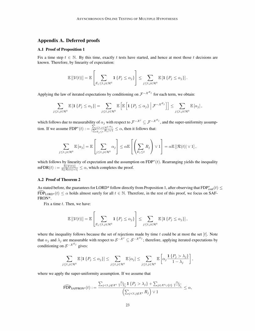
ASYNCHRONOUS ONLINE TESTING OF MULTIPLE HYPOTHESES
Appendix A. Deferred proofs
A.1 Proof of Proposition 1
Fix a time step t ∈ N. By this time, exactly t tests have started, and hence at most those t decisions areknown. Therefore, by linearity of expectation:
E [|V(t)|] = E
∑Ej≤t,j∈H0
1 {Pj ≤ αj}
≤ ∑j≤t,j∈H0
E [1 {Pj ≤ αj}] .
Applying the law of iterated expectations by conditioning on F−XEj for each term, we obtain:∑
j≤t,j∈H0
E [1 {Pj ≤ αj}] =∑
j≤t,j∈H0
E[E[1 {Pj ≤ αj}
∣∣∣ F−XEj]]≤
∑j≤t,j∈H0
E [αj ] ,
which follows due to measurability of αj with respect toF−X j ⊆ F−XEj , and the super-uniformity assump-
tion. If we assume FDP∗(t) : =∑
j≤t,j∈H0 αj
(∑
Ej≤t Rj)∨1 ≤ α, then it follows that:
∑j≤t,j∈H0
E [αj ] = E
∑j≤t,j∈H0
αj
≤ αE∑
Ej≤t
Rj
∨ 1
= αE [|R(t)| ∨ 1] ,
which follows by linearity of expectation and the assumption on FDP∗(t). Rearranging yields the inequalitymFDR(t) : = E[|V(t)|]
E[|R(t)|∨1] ≤ α, which completes the proof.
A.2 Proof of Theorem 2
As stated before, the guarantees for LORD* follow directly from Proposition 1, after observing that FDP∗conf(t) ≤FDPLORD*(t) ≤ α holds almost surely for all t ∈ N. Therefore, in the rest of this proof, we focus on SAF-FRON*.
Fix a time t. Then, we have:
E [|V(t)|] = E
∑Ej≤t,j∈H0
1 {Pj ≤ αj}
≤ ∑j≤t,j∈H0
E [1 {Pj ≤ αj}] ,
where the inequality follows because the set of rejections made by time t could be at most the set [t]. Notethat αj and λj are measurable with respect to S−X j ⊆ S−X
Ej ; therefore, applying iterated expectations byconditioning on S−X
Ej gives:
∑j≤t,j∈H0
E [1 {Pj ≤ αj}] ≤∑
j≤t,j∈H0
E [αj ] ≤∑
j≤t,j∈H0
E[αj
1 {Pj > λj}1− λj
],
where we apply the super-uniformity assumption. If we assume that
FDPSAFFRON*(t) : =
∑j<t,j 6∈X t
αj
1−λj1 {Pj > λj}+
∑j∈X t∪{t}
αj
1−λj(∑j<t,j 6∈X t Rj
)∨ 1
≤ α,
23

ZRNIC, RAMDAS, AND JORDAN
then it follows that:∑j≤t,j∈H0
E[αj
1 {Pj > λj}1− λj
]≤∑j≤t
E[αj
1 {Pj > λj}1− λj
]
≤ E
∑j<t,j 6∈X t
αj1− λj
1 {Pj > λj}+∑
j∈X t∪{t}
αj1− λj
≤ αE ∑
j<t,j 6∈X t
Rj
∨ 1
≤ αE [|R(t)| ∨ 1] ,
where the first inequality drops the condition j ∈ H0, the second one ignores the condition 1 {Pj > λj} forsome terms, the third inequality applies the assumption on FDPSAFFRON*(t) and the last inequality uses thefact thatR(t) contains all past rejections that are no longer conflicting. Rearranging the terms in the previousderivation, we reach the conclusion that mFDR(t) ≤ α, which concludes the proof of the theorem.
A.3 Proof of Theorem 3
We first prove the theorem for LORD*, and then we move on to proving the SAFFRON* guarantees.
LORD*. For all t ∈ N, define the process A(t) as:
A(t) : = −∑
i≤t,i∈H0
1 {Ei ≤ t} (1 {Pi ≤ αi} − αi) = A(t− 1)−∑
i≤t,i∈H0
1 {Ei = t} (1 {Pi ≤ αi} − αi),
where we take A(0) = 0. Let H(t) : = 1 {T ≥ t}. Since T is a stopping time, it holds that {T ≥ t + 1} =
{T ≤ t}c ∈ F−X t+1
, therefore H(t + 1) is predictable, that is it is measurable with respect to F−X t+1
.Define the transform (H ·A) of H by A as follows:
(H ·A)(t) : =
t∑m=1
H(m)(A(m)−A(m− 1))
=
t∑m=1
H(m)
− ∑i≤m,i∈H0
1 {Ei = m} (1 {Pi ≤ αi} − αi)
.
By taking conditional expectations, we can obtain:
E[(H ·A)(t+ 1)
∣∣∣ F−X t+1]
= E[(H ·A)(t)
∣∣∣ F−X t+1]
+ E[H(t+ 1)(A(t+ 1)−A(t))
∣∣∣ F−X t+1]
= E[(H ·A)(t)
∣∣∣ F−X t+1]
+H(t+ 1)E
− ∑i≤t+1,i∈H0
1 {Ei = t+ 1} (1 {Pi ≤ αi} − αi)
∣∣∣∣∣∣ F−X t+1
= E
[(H ·A)(t)
∣∣∣ F−XEt]
+H(t+ 1)∑
i≤t+1,i∈H0
1 {Ei = t+ 1}E[−(1 {Pi ≤ αi} − αi)
∣∣∣ F−X t+1],
where the first and last equality follow by linearity of expectation, and the second one uses the predictabilityof H(t+ 1). Now we can apply the super-uniformity condition (3), since we are summing over null indices:E[−1 {Pi ≤ αi}+ αi
∣∣∣ F−XEi]≥ −αi + αi = 0. Therefore, additionally applying the law of iterated
24

ASYNCHRONOUS ONLINE TESTING OF MULTIPLE HYPOTHESES
expectations, it follows that E [(H ·A)(t+ 1)] ≥ E [(H ·A)(t)]. Iteratively applying the same argument, wereach the conclusion that, for all t ∈ N:
E [(H ·A)(t)] ≥ 0. (10)
So far we have only used the predictability of H(t); observe that, by its definition, and the definition ofA(t), (H · A)(t) = A(T ∧ t) − A(0) = A(T ∧ t), and hence by equation (10), we obtain E [(H ·A)(t)] =E [A(T ∧ t)] ≥ 0.
Since A(T ∧ t)→ A(T ) almost surely as t→∞, by boundedness of T and dominated convergence wecan conclude that E [A(T ∧ t)]→ E [A(T )] as t→∞. With this we obtain a useful intermediate result:
E [A(T )] ≥ 0. (11)
Recall thatR(t) denotes the set of all rejections made by time t, and V(t) denotes the set of false rejectionsmade by time t. Consider the following process:
B(t) : = α(|R(t)| ∨ 1)− |V(t)|+∑j≤t
αj − α
∑j<t,j 6∈X t
Rj ∨ 1
≥ −|V(t)|+
∑j≤t
αj ≥ A(t),
where the final inequality applies the definition ofA(t) together with the fact that∑j≤t αj ≥
∑j≤t 1 {Ej ≤ t}αj .
Now take a stopping time T such that the conditions of the theorem are satisfied, then:
E [α(|R(T )| ∨ 1)− |V(T )|] = E
B(T )−∑j≤T
αj + α
∑j<T,j 6∈XT
Rj ∨ 1
≥ E [B(T )] ≥ E [A(T )] ≥ 0,
where the first inequality follows by definition of the LORD* FDP estimate, the second one by the relationshipalready established between A(t) and B(t), and the third inequality applies the intermediate result (11).Rearranging the terms we have that mFDR(T ) ≤ α, as desired.
SAFFRON*. We begin the proof using similar tools as in the LORD* section of the proof. For all t ∈ N,define the process A(t) as:
A(t) : = −∑
i≤t,i∈H0
1 {Ei ≤ t}(1 {Pi ≤ αi} − 1 {Pi > λi}
αi1− λi
)
= A(t− 1)−∑
i≤t,i∈H0
1 {Ei = t}(1 {Pi ≤ αi}+ 1 {Pi > λi}
αi1− λi
),
where we take A(0) = 0. Let H(t) : = 1 {T ≥ t}. Since T is a stopping time, it holds that {T ≥ t + 1} =
{T ≤ t}c ∈ F−X t+1
, therefore H(t + 1) is measurable with respect to F−X t+1
. Define the followingtransform of H by A:
(H ·A)(t) : =
t∑m=1
H(m)(A(m)−A(m− 1))
=
t∑m=1
H(m)
− ∑i≤m,i∈H0
1 {Ei = m}(1 {Pi ≤ αi}+ 1 {Pi > λi}
αi1− λi
) .
25

ZRNIC, RAMDAS, AND JORDAN
By taking conditional expectations, we can obtain:
E[(H ·A)(t+ 1)
∣∣∣ F−X t+1]
= E[(H ·A)(t)
∣∣∣ F−X t+1]
+ E[H(t+ 1)(A(t+ 1)−A(t))
∣∣∣ F−X t+1]
= E[(H ·A)(t)
∣∣∣ F−X t+1]
+H(t+ 1)E
− ∑i≤t+1,i∈H0
1 {Ei = t+ 1}(1 {Pi ≤ αi}+ 1 {Pi > λi}
αi1− λi
) ∣∣∣∣∣∣ F−X t+1
= E
[(H ·A)(t)
∣∣∣ F−X t+1]
+H(t+ 1)∑
i≤t+1,i∈H0
1 {Ei = t+ 1}E[−(1 {Pi ≤ αi}+ 1 {Pi > λi}
αi1− λi
) ∣∣∣∣ F−X t+1
],
where the first equality follows by linearity of expectation and the definition of the transform and the secondone uses measurability of H(t+1). The term−1 {Ei = t+ 1} (1 {Pi ≤ αi}+1 {Pi > λi} αi
1−λi) is clearly
non-negative when Ei 6= t + 1. If Ei = t + 1 however, we can invoke the super-uniformity condition (3),since we are summing over null indices:
E[−(1 {Pi ≤ αi}+ 1 {Pi > λi}
αi1− λi
)
∣∣∣∣ F−XEi
]≥ −αi + (1− λi)
αi1− λi
= 0.
Therefore, additionally applying the law of iterated expectations, it follows that E [(H ·A)(t+ 1)] ≥ E [(H ·A)(t)].Iteratively applying the same argument, we reach the conclusion that, for all t ∈ N:
E [(H ·A)(t)] ≥ 0. (12)
So far we have only used the predictability of H(t); observe that, by its definition, and the definition ofA(t), (H · A)(t) = A(T ∧ t) − A(0) = A(T ∧ t), and hence by equation (12), we obtain E [(H ·A)(t)] =E [A(T ∧ t)] ≥ 0.
Since A(T ∧ t)→ A(T ) almost surely as t→∞, by boundedness of T and dominated convergence wecan conclude that E [A(T ∧ t)]→ E [A(T )] as t→∞. As in the LORD* argument, we reach the result thatstates:
E [A(T )] ≥ 0. (13)
Recall R(t), the set of all rejections made by time t, and V(t), the set of false rejections made by time t.Consider the following process:
B(t) : = α(|R(t)| ∨ 1)− |V(t)|+∑
j<t,j 6∈X t
1 {Pj > λj}αj
1− λj+
∑j∈X t∪{t}
αj
1− λj−
∑j<t,j 6∈X t
Rj ∨ 1
α
≥ −|V(t)|+∑j≤t
1 {Pj > λj}αj
1− λj≥ A(t),
where the second inequality applies the definition of A(t) together with 1 {Ej ≤ t} ≤ 1.Now taking a stopping time T that satisfies the conditions of the theorem, we have:
E [α(|R(t)| ∨ 1)− |V(t)|]
= E
B(T )−∑
j<T,j 6∈XT
1 {Pj > λj}αj
1− λj−
∑j∈XT∪{T}
αj1− λj
+
∑j<T,j 6∈XT
Rj ∨ 1
α
≥ E [B(T )] ≥ E [A(T )] ≥ 0,
26

ASYNCHRONOUS ONLINE TESTING OF MULTIPLE HYPOTHESES
where the first inequality follows by construction of the SAFFRON* empirical FDP estimate, the secondinequality uses the proved relationship betweenA(t) andB(t), and the third inequality applies equation (13).Rearranging the terms we have that mFDR(T ) ≤ α, as desired.
A.4 Proof of Lemma 4
We begin by focusing on the first inequality. Letting P1:M = (P1, . . . , PM ) be the original vector of p-values,we define a “hallucinated” vector of p-values P t→1
1:M : = (P1, . . . , PM ) that equals P1:M , except that the t-thcomponent is set to one:
Pi =
{1 if i = t,Pi if i 6= t.
Further, denote by Ej the finish times of the tests that yield Pj , and let Ej be equal to Ej for all 1 ≤j ≤ M . Denote the set of candidates and rejections in the hallucinated sequence at time i by Ci and Ri,respectively, and let αi be the test level for Pi. Also, letR1:M = (R1, . . . ,RM ) and Rt→1
1:M = (R1, . . . , RM )
denote the vectors of the numbers of rejections using P1:M and P t→11:M , respectively. Similarly, let C1:M =
(C1, . . . , CM ) and Ct→11:M = (C1, . . . , CM ) denote the vectors of the numbers of candidates using P1:M and
P t→11:M , respectively.
By construction, we have the following properties:
1. Ej = Ej ,∀j implies αi = αi for all i ≤ Et.
2. Ri = Ri and Ci = Ci for all i < Et, since the p-values from the finished tests and the respective testlevels are the same in the original and hallucinated setting.
3. REt ⊆ REt and CEt ⊆ CEt , and hence Ri ⊆ Ri also for all i > Et, due to monotonicity of the testlevels αi and candidacy thresholds λi.
Therefore, on the event {Pt > λt}, we haveREt= REt
and CEt= CEt
, and hence alsoR1:M = Rt→11:M and
C1:M = Ct→11:M . This allows us to conclude that:
αt1 {Pt > λt}(1− λt)g(|R|1:M )
=αt1 {Pt > λt}
(1− λt)g(|R|t→11:M )
.
Since the null p-values are mutually independent and independent of the non-nulls, we conclude thatRt→1
1:M is independent of Pt conditioned on F−XEt
async . With this, we can obtain:
E[
αt1 {Pt > λt}(1− λt)g(|R|1:M )
∣∣∣∣ F−XEt
async
]= E
[αt1 {Pt > λt}
(1− λt)g(|R|t→11:M )
∣∣∣∣∣ F−XEt
async
]≥ E
[αt
g(|R|t→11:M )
∣∣∣∣∣ F−XEt
async
]
≥ E[
αtg(|R|1:M )
∣∣∣∣ F−XEt
async
],
where the first inequality follows by taking an expectation only with respect to Pt by invoking the asyn-chronous super-uniformity property (6), and the second inequality follows because g(|R|1:M ) ≥ g(|R|t→1
1:M )
since |Ri| ≥ |Ri| for all i by monotonicity of the test levels and candidacy thresholds. This concludes theproof of the first inequality.
The second inequality uses a similar idea of hallucinating tests with identical finish times, only now thep-values that these tests result in are:
Pi =
{0 if i = t,Pi if i 6= t,
where Pi are the p-values in the original sequence. In a similar fashion, the following observations hold:
27

ZRNIC, RAMDAS, AND JORDAN
1. Ej = Ej implies αi = αi for all i ≤ Et.
2. Ri = Ri and Ci = Ci for all i < Et, since the p-values from the finished tests and the respective testlevels are the same in the original and hallucinated setting.
3. REt⊇ REt
and CEt⊇ CEt
, and hence Ri ⊇ Ri also for all i > Et, due to monotonicity of the testlevels αi.
Then, on the event {Pt ≤ αt}, we have REt = REt and CEt = CEt, and hence also R1:M = Rt→1
1:M andC1:M = Ct→1
1:M . From this we conclude that:
1 {Pt ≤ αt}g(|R|1:M )
=1 {Pt ≤ αt}g(|R|t→1
1:M ).
As in the first part of the proof, we use the fact that the null p-values are mutually independent andindependent of the non-nulls, which allows us to conclude that Rt→1
1:M is independent of Pt conditioned onFXEt
async . This observation results in the following:
E[1 {Pt ≤ αt}g(|R|1:M )
∣∣∣∣ FXEt
async
]= E
[1 {Pt ≤ αt}g(|R|t→1
1:M )
∣∣∣∣∣ FXEt
async
]≤ E
[αt
g(|R|t→11:M )
∣∣∣∣∣ FXEt
async
]
≤ E[
αtg(|R|1:M )
∣∣∣∣ FXEt
async
],
where the first inequality follows by taking an expectation only with respect to Pt by invoking the asyn-chronous super-uniformity property (6), and the second inequality follows because g(|R|1:M ) ≤ g(|R|t→1
1:M )
since |Ri| ≤ |Ri| for all i by monotonicity of the test levels. This concludes the proof of the lemma.
A.5 Proof of Theorem 5
LORDasync. Fix a time step t. First we show the claim for LORDasync, so suppose that
FDPLORDasync(t) : =
∑j≤t αj∑
j≤t 1 {Pj ≤ αj , Ej ≤ t} ∨ 1≤ α.
Then:
FDR(t) : = E[|V(t)||R(t)| ∨ 1
]= E
[∑j≤t,j∈H0 1 {Pj ≤ αj , Ej ≤ t}∑j≤t 1 {Pj ≤ αj , Ej ≤ t} ∨ 1
]
≤∑
i≤t,i∈H0
E
[1 {Pi ≤ αi}∑
j≤t 1 {Pj ≤ αj , Ej ≤ t} ∨ 1
],
where the second equality follows by definition of V(t) and R(t), and the inequality drops the conditionEi ≤ t from the numerator and applies linearity of expectation. Now we can apply Lemma 4 with g(|R|1:t) =(∑ti=1 |Ri|) ∨ 1, together with iterated expectations, to obtain:
∑i≤t,i∈H0
E
[1 {Pi ≤ αi}∑
j≤t 1 {Pj ≤ αj , Ej ≤ t} ∨ 1
]≤
∑i≤t,i∈H0
E
[αi∑
j≤t 1 {Pj ≤ αj , Ej ≤ t} ∨ 1
]
≤ E[FDPLORDasync(t)
]≤ α,
where the second inequality follows by dropping the condition i ∈ H0. This completes the proof forLORDasync.
28

ASYNCHRONOUS ONLINE TESTING OF MULTIPLE HYPOTHESES
SAFFRONasync. Now we move on to SAFFRONasync. Using the same steps as above, for any fixed time t,we can conclude the following inequality:
FDR(t) ≤∑
i≤t,i∈H0
E
[αi∑
j≤t 1 {Pj ≤ αj , Ej ≤ t} ∨ 1
].
Here we additionally apply the other inequality of Lemma 4, with the same choice g(|R|1:t) = (∑ti=1 |Ri|)∨
1, again with iterated expectations:
∑i≤t,i∈H0
E
[αi∑
j≤t 1 {Pj ≤ αj , Ej ≤ t} ∨ 1
]≤
∑i≤t,i∈H0
E
[αi1 {Pi > λi}
(1− λi)(∑j≤t 1 {Pj ≤ αj , Ej ≤ t} ∨ 1)
].
Assuming that the inequality
FDPSAFFRONasync(t) : =
∑j≤t
αj
1−λj(1 {Pj > λj , Ej ≤ t}+ 1 {Ej > t})∑j≤t 1 {Pj ≤ αj , Ej ≤ t} ∨ 1
≤ α
holds, it follows that:
∑i≤t,i∈H0
E
[αi1 {Pi > λi}
(1− λi)(∑j≤t 1 {Pj ≤ αj , Ej ≤ t} ∨ 1)
]
≤ E
[∑j≤t
αj
1−λj(1 {Pj > λj , Ej ≤ t}+ 1 {Ej > t})∑j≤t 1 {Pj ≤ αj , Ej ≤ t} ∨ 1
]= E
[FDPSAFFRONasync(t)
]≤ α,
where the first inequality follows by dropping the conditions j ∈ H0 and {Pj > λj} for some rounds. Thesecond inequality follows by assumption, hence proving the theorem.
A.6 Proof of Theorem 6
For statement (a), we begin by noting that for any t ∈ N:
FDR(t) = E[∑
i≤t,i∈H0 1 {Pi ≤ αi}|R(t)| ∨ 1
]≤
∑i≤t,i∈H0
E[
1 {Pi ≤ αi}|R(i− 1)| ∨ 1
]=
∑i≤t,i∈H0
γiαE[1 {Pi ≤ αi}
αi
],
where the first equality follows by definition of FDR, the sole inequality follows because the number ofrejections can only increase with time, and the second equality follows by definition of the LOND rule forαi. Lemma 1 from Ramdas et al. (2019) now asserts that the term in the expectation is bounded by one underPRDS. Hence, by also noting that
∑i≤t γi ≤ 1 we immediately deduce statement (a).
For statement (b), we follow almost the same sequence of steps to note that:
FDR(t) = E[∑
i≤t,i∈H0 1 {Pi ≤ αi}|R(t)| ∨ 1
]≤
∑i≤t,i∈H0
E[
1 {Pi ≤ αi}|R(i− 1)| ∨ 1
]
=∑
i≤t,i∈H0
γiαE[1 {Pi ≤ γiαβi(|R(i− 1)| ∨ 1)}
γiα(|R(i− 1)| ∨ 1)
].
We now apply Lemma 1 from Ramdas et al. (2019) with c = γiα and f(P ) = |R(i− 1)| ∨ 1 to again assertthat the term in the expectation is bounded by one under arbitrary dependence, hence establishing statement(b).
29

ZRNIC, RAMDAS, AND JORDAN
Appendix B. Different instantiations of LORD* and SAFFRON*Here we give explicit statements of different instances of LORD* and SAFFRON* described in Section 3,Section 4 and Section 5. All of the following algorithms are special instances of Algorithms 1-4, given inSection 2.
First we state LORDasync and SAFFRONasync explicitly, by takingX t = X tasync in the statement of LORD*and SAFFRON*. Algorithm 5 and Algorithm 6 state the LORD++ and LOND versions of LORDasync, Al-gorithm 7 states SAFFRONasync for constant candidacy thresholds, i.e. {λj} ≡ λ, and Algorithm 8 statesasynchronous alpha-investing, i.e. SAFFRONasync when λj = αj . Recall the definition of rk, which in thissetting takes the form:
rk = min{i ∈ [t] :
i∑j=1
Rj1 {Ej ≤ i} ≥ k}.
Algorithm 5 The asynchronous LORD++ algorithm as a version of LORDasync
input: FDR level α, non-negative non-increasing sequence {γj}∞j=1 such that∑
j γj = 1, initial wealth W0 ≤ αα1 = γ1W0
for t = 1, 2, . . . dostart t-th test with level αt
αt+1 = γt+1W0 + γt+1−r1 (α−W0) +(∑
j≥2 γt+1−rj
)α
end
Algorithm 6 The asynchronous LOND algorithm as a version of LORDasync
input: FDR level α, non-negative non-increasing sequence {γj}∞j=1 such that∑
j γj = 1W0 = αα1 = γ1W0
for t = 1, 2, . . . dostart t-th test with level αt
αt+1 = αγt+1
((∑t
j=1 1 {Pj ≤ αj , Ej ≤ t}) ∨ 1)
end
Algorithm 7 The SAFFRONasync algorithm for constant λinput: FDR level α, non-negative non-increasing sequence {γj}∞j=1 such that
∑j γj = 1, candidate threshold λ ∈ (0, 1), initial
wealth W0 ≤ αα1 = (1− λ)γ1W0
for t = 1, 2, . . . dostart t-th test with level αt
αt+1 = min
{λ, (1− λ)
(W0γt+1−C
#0+
+ (α−W0)γt+1−r1−C#1+
+∑
j≥2 αγt+1−rj−C#j+
)},
where C#j+ =
∑ti=rj+1 |Ci|
end
Algorithm 8 The asynchronous alpha-investing algorithm as a special case of SAFFRONasync
input: FDR level α, non-negative non-increasing sequence {γj}∞j=1 such that∑
j γj = 1, initial wealth W0 ≤ αs1 = γ1W0
α1 = s1/(1 + s1)for t = 1, 2, . . . do
start t-th test with level αt
st+1 =W0γt+1−R#0 +
+ (α−W0)γt+1−r1−R#1+
+∑
j≥2 αγt+1−rj−R#j+
, where R#j+ =
∑ti=rj+1 |Ri|
αt+1 = st+1/(1 + st+1)end
30

ASYNCHRONOUS ONLINE TESTING OF MULTIPLE HYPOTHESES
Below we give explicit statements of LORDdep and SAFFRONdep as special cases of LORD* and SAF-FRON*. Algorithm 9 and Algorithm 10 state LORD++ and LOND under local dependence, both as instancesof LORDdep. Algorithm 11 states SAFFRONdep for the constant sequence {λj} ≡ λ, and Algorithm 12 statesalpha-investing under local dependence, which is a particular instance of SAFFRONdep obtained by takingλj = αj . The definition of rk under local dependence simplify to:
rk = min{i ∈ [t] :
i−Li+1∑j=1
Rj ≥ k}.
Algorithm 9 The LORD++ algorithm under local dependence as a version of LORDdep
input: FDR level α, non-negative non-increasing sequence {γj}∞j=1 such that∑
j γj = 1, initial wealth W0 ≤ αα1 = γ1W0
for t = 1, 2, . . . dorun t-th test with level αt
αt+1 = γt+1W0 + γt+1−r1 (α−W0) +(∑∞
j=2 γt+1−rj
)α
end
Algorithm 10 The LOND algorithm under local dependence as a version of LORDdep
input: FDR level α, non-negative non-increasing sequence {γj}∞j=1 such that∑
j γj = 1W0 = αα1 = γ1W0
for t = 1, 2, . . . dorun t-th test with level αt
αt+1 = αγt+1
((∑t−Lt+1
i=1 Ri) ∨ 1)
end
Algorithm 11 The SAFFRONdep algorithm for constant λinput: FDR level α, non-negative non-increasing sequence {γj}∞j=1 such that
∑j γj = 1, candidate threshold λ ∈ (0, 1), initial
wealth W0 ≤ αα1 = γ1W0
for t = 1, 2, . . . dorun t-th test with level αt
αt+1 = min{λ, (1− λ)
(W0γt+1−C0+ + (α−W0)γt+1−r1−C1+
+ α(∑
j≥2 γt+1−rj−Cj+))}
,
where Cj+ =∑t−Lt+1
i=rj+1 Ci
end
Algorithm 12 The alpha-investing algorithm under local dependence as a special case of SAFFRONdep
input: FDR level α, non-negative non-increasing sequence {γj}∞j=1 such that∑
j γj = 1, initial wealth W0 ≤ αs1 = γ1W0
α1 = s1/(1 + s1)for t = 1, 2, . . . do
run t-th test with level αt
st+1 =W0γt+1−R0+ + (α−W0)γt+1−r1−R1++∑
j≥2 αγt+1−rj−Rj+, where Rj+ =
∑t−Lt+1i=rj+1 Ri
αt+1 = st+1/(1 + st+1)end
Algorithms 13 and 14 describe the mini-batch versions of LORD++ and LOND respectively, both ascases of LORDmini. Algorithm 15 is a variant of SAFFRONmini with λj chosen constant and equal to some
31

ZRNIC, RAMDAS, AND JORDAN
λ ∈ (0, 1), and Algorithm 16 is the alpha-investing version of SAFFRONmini, in which λj = αj . In thissetting, the definition of rk is slightly tweaked in order to satisfy the convention of double indexing; rk refersto the batch in which the k-th non-conflicting rejection occurs:
rk : = min{i ∈ [b− 1] :
i∑j=1
|Rj | ≥ k}.
Algorithm 13 The mini-batch LORD++ algorithm as a version of LORDmini
input: FDR level α, non-negative non-increasing sequence {γj}∞j=1 such that∑
j γj = 1, initial wealth W1,0 ≤ αα1,1 = γ1W1,0
for b = 1, 2, . . . doif b > 1 then
Wb,0 =Wb−1,n + α|Rb−1| −W1,01 {r1 = b− 1}endfor t = 1, 2, . . . , nb do
start t-th test in the b-th batch with level αb,t
αb,t+1 = γ∑b−1i=1 ni+t+1
W1,0 + γ∑b−1i=1 ni+t+1−
∑r1i=1 ni
(α−W1,0) +
(∑∞j=2 γ∑b−1
i=1 ni+t+1−∑rj
i=1 ni
)α
endend
Algorithm 14 The mini-batch LOND algorithm as a version of LORDmini
input: FDR level α, non-negative non-increasing sequence {γj}∞j=1 such that∑
j γj = 1α1,1 = γ1α
for b = 1, 2, . . . dofor t = 1, 2, . . . , nb do
start t-th test in the b-th batch with level αb,t
αb,t+1 = αγ∑b−1i=1 ni+t+1
((∑b−1
j=1 |Rj |) ∨ 1)
endend
Algorithm 15 The SAFFRONmini algorithm for constant λinput: FDR level α, non-negative non-increasing sequence {γj}∞j=1 such that
∑j γj = 1, initial wealth W1,0 ≤ α, constant λ
α1,1 = (1− λ)γ1W1,0
for b = 1, 2, . . . dofor t = 1, 2, . . . , n do
start t-th test in the b-th batch with level αb,t
αb,t+1 = (1 − λ)(γ∑b−1i=1 ni−|C
+0 |+t+1
W1,0 + γ∑b−1i=1 ni−|C
+1 |+t+1−
∑r1i=1 ni
(α − W1,0) +(∑∞j=2 γ∑b−1
i=1 ni−|C+j |+t+1−
∑r1i=1 ni
)α), where |C+j | =
∑b−1j=rj+1 |Cj |
endend
32

ASYNCHRONOUS ONLINE TESTING OF MULTIPLE HYPOTHESES
Algorithm 16 The mini-batch alpha-investing as a special case of SAFFRONmini
input: FDR level α, non-negative non-increasing sequence {γj}∞j=1 such that∑
j γj = 1, initial wealth W1,0 ≤ αs1,1 = γ1W1,0
α1,1 = s1,1/(1 + s1,1)for b = 1, 2, . . . do
for t = 1, 2, . . . , n dostart t-th test in the b-th batch with level αb,t
sb,t+1 = γ∑b−1i=1 ni−|C
+0 |+t+1
W1,0 + γ∑b−1i=1 ni−|C
+1 |+t+1−
∑r1i=1 ni
(α − W1,0) +(∑∞j=2 γ∑b−1
i=1 ni−|C+j |+t+1−
∑rji=1 ni
)α, where |C+j | =
∑b−1j=rj+1 |Cj |
αb,t+1 = sb,t+1/(1 + sb,t+1)
endend
Appendix C. Experiments on real data with local dependence
We perform an additional case study on a high-throughput phenotypic data set from the International MousePhenotyping Consortium (IMPC) data repository. This database documents gene knockout experiments onmice and annotates every protein coding gene by exploring the impact of the gene knockout on the resultingphenotype. This is an example of a continuously growing data set, as the family of hypotheses and the newknockouts grow with time. Karp et al. (2017) tested the role of genotype and the role of sex as a modifier ofgenotype effect. In this section, we focus on the p-values resulting from the analysis of genotype effects. Thisset of p-values exhibits local dependence—the same set of mice is used to test multiple hypotheses adjacenton the time horizon, while p-values computed at sufficiently distant time points are statistically independent.
We use the subset of the database organized by Robertson et al. (2019), which is available at https://zenodo.org/record/2396572.Hypotheses belonging to the same batch have the same experimental ID. For the sake of computational ef-ficiency, we only analyze the hypotheses whose experimental ID is in the interval [36700, 37000). Thisresults in 4275 distinct hypotheses and their corresponding p-values, split into 172 batches of varying sizes.For different target FDR levels, we report the number of discoveries made by SAFFRONdep, LORDdep, andalpha-spending. Since we expect a small number of truly relevant genes, for SAFFRONdep we set λ = 0.1;all other parameters for all three algorithms are as in Section 7. We cannot evaluate the FDR and power dueto lack of ground truth, but theoretically all three procedures control the FDR at the target level.
0.05 0.10 0.15 0.20 0.25 0.30 0.35 0.40
FDR level
0
200
400
600
800
num
ber
ofre
ject
ion
s
SAFFRONdep
LORDdep
Alpha-spending
Figure 12: Number of rejections made by SAFFRONdep, LORDdep, and alpha-spending, for different targetFDR levels.
33

ZRNIC, RAMDAS, AND JORDAN
Appendix D. Additional experiments with varying asynchrony
We illustrate the tradeoff between the power gain of optimized tests, which make use of the test level αi atthe beginning of the test, and the accompanying power loss when running such tests asynchronously. We doso by contrasting optimized sequential tests with their simpler counterparts which compute p-values withoutknowledge of αi in a simulated A/B testing environment.
We test null hypotheses of the formHi : µ(i)treatment−µ
(i)control = 0, and for each test we collect samples from
N(µ(i)control, 1) and N(µ
(i)treatment, 1). We collect samples by uniformly sampling from the treatment and control
distribution; at every sampling step j of test i we draw a single sample from both distributions, X(i,j)treatment ∼
N(µ(i)treatment, 1),X(i,j)
control ∼ N(µ(i)control, 1), akin to allocating one of two matched patients to each of those arms.
We contrast two approaches: in one, we fix the number of per-test draws n from each distribution, and simplycalculate a p-value by computing Pi = 1−Φ(
√n/2(µ
(i)treatment−µ
(i)control)), where µ(i)
treatment = 1n
∑nj=1X
(i,j)treatment
and µ(i)control = 1
n
∑nj=1X
(i,j)control. This approach does not require an asynchronous correction. In the other
approach, we use the test level αi and the law of the iterated logarithm to adaptively stop sample collectiononce a rejection is admissible; as in the first approach, we collect at most n samples from each distribution,but we stop and make a rejection after k ≤ n draws if
k∑j=1
(X
(i,j)treatment −X
(i,j)control
)>√k(4 log(1/(αi ∧ 0.1)) + 12 log(log(1/(αi ∧ 0.1))) + 6 log(log(ek))).
Validity of this stopping rule follows from Theorem 8 in Kaufmann et al. (2016). For other stopping rulesthat can be employed in nonparametric situations, see Howard et al. (2021).
Rather than fixing the total number of tests, we fix the total sample budget B. In the simpler strategy, thiscorresponds to fixing the total number of tests one can perform, namely bB/(2n)c. In the adaptive approach,the number of tests is lower bounded by bB/(2n)c, but can be higher if rejections are made with fewer thann samples drawn per distribution.
For each test, with equal probability we let µ(i)treatment − µ
(i)control = 0, in which case the null hypothesis is
true, or we draw the margin from an exponential distribution, µ(i)treatment − µ
(i)control ∼ Exp(1), in which case the
null is false. We set α = 0.05 and average all results over 200 trials. In each trial, all considered algorithmsobserve the same sequence of average treatment effects, {µ(i)
treatment−µ(i)control}, but draw independent Gaussian
samples. In Figure 13, we plot the number of true discoveries made by LORD against different values of thesample budget B for several different values of n (varying n changes the false negative rate). The adaptivestopping strategy with a low level of asynchrony generally outperforms the naive approach; however, if thelevel of asynchrony is high (relative to other problem parameters), the naive approach dominates, as expected.
Appendix E. Positive regression dependency on a subset (PRDS)
We briefly review the definition of positive regression dependency on a subset (PRDS).
Definition 7 Let D ⊆ [0, 1]n be any non-decreasing set, meaning that x ∈ D implies y ∈ D, for all ysuch that yi ≥ xi for all i ∈ [n]. We say that a vector of p-values P = (P1, . . . , Pn) satisfies positivedependence (PRDS) if for any null index i ∈ H0 and arbitrary non-decreasing D ⊆ [0, 1]n, the functiont→ Pr{P ∈ D | Pi ≤ t} is non-decreasing over t ∈ (0, 1].
Clearly, independent p-values satisfy PRDS. Another important example is given for Gaussian obser-vations. Suppose Z = (Z1, . . . , Zn) is a multivariate Gaussian with covariance matrix Σ, and let P =(Φ(Z1, ), . . . ,Φ(Zn)) be a vector of p-values, where Φ is the standard Gaussian CDF. Then, P satisfiesPRDS if and only if, for all i ∈ H0 and j ∈ [n], Σij ≥ 0.
34

ASYNCHRONOUS ONLINE TESTING OF MULTIPLE HYPOTHESES
50000 100000 150000 200000 250000
sample budget
50
100
150
200
num
ber
oftr
ue
reje
ctio
ns
LORD w/ simple p-values
LORDasync, p = 1/50
LORDasync, p = 1/500
LORDasync, p = 1/1000
50000 100000 150000 200000 250000
sample budget
25
50
75
100
125
num
ber
oftr
ue
reje
ctio
ns
LORD w/ simple p-values
LORDasync, p = 1/50
LORDasync, p = 1/500
LORDasync, p = 1/1000
50000 100000 150000 200000 250000
sample budget
20
40
60
80
100
num
ber
oftr
ue
reje
ctio
ns
LORD w/ simple p-values
LORDasync, p = 1/50
LORDasync, p = 1/500
LORDasync, p = 1/1000
Figure 13: Number of true discoveries made by LORD with simple p-values and LORDasync with a sequentialstrategy, against the sample budgetB. The values of n are 400 (left), 800 (middle), 1200 (right). The durationof asynchronous tests is sampled as in Section 7.
Appendix F. Examining the difference between mFDR and FDR
In Section 7, we plotted strict FDR estimates, obtained by averaging the false discovery proportion over200 independent trials; on the other hand, the main guarantees of this paper apply to mFDR control. Forthis reason, here we provide the plot of both mFDR and FDR estimates, for all experiments in Section 7.We estimate mFDR by computing the ratio of the average number of false discoveries and the average totalnumber of discoveries.
0.0 0.1 0.2 0.3 0.4 0.5 0.6 0.7 0.8 0.9
π1
0.0
0.1
0.2
0.3
0.4
0.5
0.6
0.7
0.8
0.9
1.0
FD
R
LORDasync, p = 1
LORDasync, p = 1/50
LORDasync, p = 1/100
LORDasync, p = 1/150
Alpha-spending
Uncorrected
0.0 0.1 0.2 0.3 0.4 0.5 0.6 0.7 0.8 0.9
π1
0.0
0.1
0.2
0.3
0.4
0.5
0.6
0.7
0.8
0.9
1.0
mF
DR
LORDasync, p = 1
LORDasync, p = 1/50
LORDasync, p = 1/100
LORDasync, p = 1/150
Alpha-spending
Uncorrected
0.0 0.1 0.2 0.3 0.4 0.5 0.6 0.7 0.8 0.9
π1
0.0
0.1
0.2
0.3
0.4
0.5
0.6
0.7
0.8
0.9
1.0
FD
R
SAFFRONasync, p = 1
SAFFRONasync, p = 1/50
SAFFRONasync, p = 1/100
SAFFRONasync, p = 1/150
Alpha-spending
Uncorrected
0.0 0.1 0.2 0.3 0.4 0.5 0.6 0.7 0.8 0.9
π1
0.0
0.1
0.2
0.3
0.4
0.5
0.6
0.7
0.8
0.9
1.0
mF
DR
SAFFRONasync, p = 1
SAFFRONasync, p = 1/50
SAFFRONasync, p = 1/100
SAFFRONasync, p = 1/150
Alpha-spending
Uncorrected
0.0 0.1 0.2 0.3 0.4 0.5 0.6 0.7 0.8 0.9
π1
0.0
0.1
0.2
0.3
0.4
0.5
0.6
0.7
0.8
0.9
1.0
FD
R
SAFFRONasync, p = 1
SAFFRONasync, p = 1/50
SAFFRONasync, p = 1/100
SAFFRONasync, p = 1/150
Alpha-spending
Uncorrected
0.0 0.1 0.2 0.3 0.4 0.5 0.6 0.7 0.8 0.9
π1
0.0
0.1
0.2
0.3
0.4
0.5
0.6
0.7
0.8
0.9
1.0
mF
DR
SAFFRONasync, p = 1
SAFFRONasync, p = 1/50
SAFFRONasync, p = 1/100
SAFFRONasync, p = 1/150
Alpha-spending
Uncorrected
Figure 14: The left plots reproduce FDR from Figure 5 and Figure 6, while the right plots show mFDR forthe same experiments.
35

ZRNIC, RAMDAS, AND JORDAN
0.0 0.1 0.2 0.3 0.4 0.5 0.6 0.7 0.8 0.9
π1
0.0
0.1
0.2
0.3
0.4
0.5
0.6
0.7
0.8
0.9
1.0
FD
RLORDdep, L = 0
LORDdep, L = 50
LORDdep, L = 100
LORDdep, L = 150
Alpha-spending
Uncorrected
0.0 0.1 0.2 0.3 0.4 0.5 0.6 0.7 0.8 0.9
π1
0.0
0.1
0.2
0.3
0.4
0.5
0.6
0.7
0.8
0.9
1.0
mF
DR
LORDdep, L = 0
LORDdep, L = 50
LORDdep, L = 100
LORDdep, L = 150
Alpha-spending
Uncorrected
0.0 0.1 0.2 0.3 0.4 0.5 0.6 0.7 0.8 0.9
π1
0.0
0.1
0.2
0.3
0.4
0.5
0.6
0.7
0.8
0.9
1.0
FD
R
LORDdep, L = 0
LORDdep, L = 50
LORDdep, L = 100
LORDdep, L = 150
Alpha-spending
Uncorrected
0.0 0.1 0.2 0.3 0.4 0.5 0.6 0.7 0.8 0.9
π1
0.0
0.1
0.2
0.3
0.4
0.5
0.6
0.7
0.8
0.9
1.0
mF
DR
LORDdep, L = 0
LORDdep, L = 50
LORDdep, L = 100
LORDdep, L = 150
Alpha-spending
Uncorrected
0.0 0.1 0.2 0.3 0.4 0.5 0.6 0.7 0.8 0.9
π1
0.0
0.1
0.2
0.3
0.4
0.5
0.6
0.7
0.8
0.9
1.0
FD
R
SAFFRONdep, L = 0
SAFFRONdep, L = 50
SAFFRONdep, L = 100
SAFFRONdep, L = 150
Alpha-spending
Uncorrected
0.0 0.1 0.2 0.3 0.4 0.5 0.6 0.7 0.8 0.9
π1
0.0
0.1
0.2
0.3
0.4
0.5
0.6
0.7
0.8
0.9
1.0
mF
DR
SAFFRONdep, L = 0
SAFFRONdep, L = 50
SAFFRONdep, L = 100
SAFFRONdep, L = 150
Alpha-spending
Uncorrected
0.0 0.1 0.2 0.3 0.4 0.5 0.6 0.7 0.8 0.9
π1
0.0
0.1
0.2
0.3
0.4
0.5
0.6
0.7
0.8
0.9
1.0
FD
R
SAFFRONdep, L = 0
SAFFRONdep, L = 50
SAFFRONdep, L = 100
SAFFRONdep, L = 150
Alpha-spending
Uncorrected
0.0 0.1 0.2 0.3 0.4 0.5 0.6 0.7 0.8 0.9
π1
0.0
0.1
0.2
0.3
0.4
0.5
0.6
0.7
0.8
0.9
1.0
mF
DR
SAFFRONdep, L = 0
SAFFRONdep, L = 50
SAFFRONdep, L = 100
SAFFRONdep, L = 150
Alpha-spending
Uncorrected
Figure 15: The left plots reproduce FDR from Figure 7 and Figure 8, while the right plots show mFDR forthe same experiments.
0.0 0.1 0.2 0.3 0.4 0.5 0.6 0.7 0.8 0.9
π1
0.0
0.1
0.2
0.3
0.4
0.5
0.6
0.7
0.8
0.9
1.0
FD
R
LORDmini, B = 1
LORDmini, B = 50
LORDmini, B = 100
LORDmini, B = 150
Alpha-spending
Uncorrected
0.0 0.1 0.2 0.3 0.4 0.5 0.6 0.7 0.8 0.9
π1
0.0
0.1
0.2
0.3
0.4
0.5
0.6
0.7
0.8
0.9
1.0
mF
DR
LORDmini, B = 1
LORDmini, B = 50
LORDmini, B = 100
LORDmini, B = 150
Alpha-spending
Uncorrected
0.0 0.1 0.2 0.3 0.4 0.5 0.6 0.7 0.8 0.9
π1
0.0
0.1
0.2
0.3
0.4
0.5
0.6
0.7
0.8
0.9
1.0
FD
R
SAFFRONmini, B = 1
SAFFRONmini, B = 50
SAFFRONmini, B = 100
SAFFRONmini, B = 150
Alpha-spending
Uncorrected
0.0 0.1 0.2 0.3 0.4 0.5 0.6 0.7 0.8 0.9
π1
0.0
0.1
0.2
0.3
0.4
0.5
0.6
0.7
0.8
0.9
1.0
mF
DR
SAFFRONmini, B = 1
SAFFRONmini, B = 50
SAFFRONmini, B = 100
SAFFRONmini, B = 150
Alpha-spending
Uncorrected
0.0 0.1 0.2 0.3 0.4 0.5 0.6 0.7 0.8 0.9
π1
0.0
0.1
0.2
0.3
0.4
0.5
0.6
0.7
0.8
0.9
1.0
FD
R
SAFFRONmini, B = 1
SAFFRONmini, B = 50
SAFFRONmini, B = 100
SAFFRONmini, B = 150
Alpha-spending
Uncorrected
0.0 0.1 0.2 0.3 0.4 0.5 0.6 0.7 0.8 0.9
π1
0.0
0.1
0.2
0.3
0.4
0.5
0.6
0.7
0.8
0.9
1.0
mF
DR
SAFFRONmini, B = 1
SAFFRONmini, B = 50
SAFFRONmini, B = 100
SAFFRONmini, B = 150
Alpha-spending
Uncorrected
Figure 16: The left plots reproduce FDR from Figure 9 and Figure 10, while the right plots show mFDR forthe same experiments.
36

ASYNCHRONOUS ONLINE TESTING OF MULTIPLE HYPOTHESES
0.0 0.1 0.2 0.3 0.4 0.5 0.6 0.7 0.8 0.9
π1
0.0
0.1
0.2
0.3
0.4
0.5
0.6
0.7
0.8
0.9
1.0
FD
RSAFFRONdep
LORDdep
LORD under dependence
Alpha-spending
Uncorrected
0.0 0.1 0.2 0.3 0.4 0.5 0.6 0.7 0.8 0.9
π1
0.0
0.1
0.2
0.3
0.4
0.5
0.6
0.7
0.8
0.9
1.0
mF
DR
SAFFRONdep
LORDdep
LORD under dependence
Alpha-spending
Uncorrected
0.0 0.1 0.2 0.3 0.4 0.5 0.6 0.7 0.8 0.9
π1
0.0
0.1
0.2
0.3
0.4
0.5
0.6
0.7
0.8
0.9
1.0
FD
R
SAFFRONdep
LORDdep
LORD under dependence
Alpha-spending
Uncorrected
0.0 0.1 0.2 0.3 0.4 0.5 0.6 0.7 0.8 0.9
π1
0.0
0.1
0.2
0.3
0.4
0.5
0.6
0.7
0.8
0.9
1.0
mF
DR
SAFFRONdep
LORDdep
LORD under dependence
Alpha-spending
Uncorrected
Figure 17: The left plots reproduce FDR from Figure 11, while the right plots show mFDR for the sameexperiments.
ReferencesEhud Aharoni and Saharon Rosset. Generalized α-investing: definitions, optimality results and application
to public databases. Journal of the Royal Statistical Society, Series B (Statistical Methodology), pages771–794, 2014.
Arthur E Albert. The sequential design of experiments for infinitely many states of nature. The Annals ofMathematical Statistics, pages 774–799, 1961.
Akshay Balsubramani and Aaditya Ramdas. Sequential nonparametric testing with the law of the iteratedlogarithm. In Proceedings of the 32nd Conference on Uncertainty in Artificial Intelligence, 2016.
Jay Bartroff and Tze Leung Lai. Generalized likelihood ratio statistics and uncertainty adjustments in efficientadaptive design of clinical trials. Sequential Analysis, 27(3):254–276, 2008.
Jay Bartroff and Jinlin Song. Sequential tests of multiple hypotheses controlling type I and II familywiseerror rates. Journal of statistical planning and inference, 153:100–114, 2014.
Jay Bartroff, Tze Leung Lai, and Mei-Chiung Shih. Sequential experimentation in clinical trials: design andanalysis, volume 298. Springer Science & Business Media, 2012.
Raef Bassily, Kobbi Nissim, Adam Smith, Thomas Steinke, Uri Stemmer, and Jonathan Ullman. Algorithmicstability for adaptive data analysis. In Proceedings of the 48th Annual ACM Symposium on Theory ofComputing, pages 1046–1059. ACM, 2016.
Yoav Benjamini and Yosef Hochberg. Controlling the false discovery rate: a practical and powerful approachto multiple testing. Journal of the Royal Statistical Society, Series B (Methodological), 57(1):289–300,1995.
Yoav Benjamini and Daniel Yekutieli. The control of the false discovery rate in multiple testing underdependency. Annals of Statistics, pages 1165–1188, 2001.
Gilles Blanchard and Etienne Roquain. Two simple sufficient conditions for FDR control. Electronic Journalof Statistics, 2:963–992, 2008.
Avrim Blum and Moritz Hardt. The Ladder: A reliable leaderboard for machine learning competitions. InProceedings of the 32nd International Conference on Machine Learning, pages 1006–1014, 2015.
Herman Chernoff. Sequential design of experiments. The Annals of Mathematical Statistics, 30(3):755–770,1959.
37

ZRNIC, RAMDAS, AND JORDAN
Cynthia Dwork, Vitaly Feldman, Moritz Hardt, Toniann Pitassi, Omer Reingold, and Aaron Roth. Thereusable holdout: Preserving validity in adaptive data analysis. Science, 349(6248):636–638, 2015a.
Cynthia Dwork, Vitaly Feldman, Moritz Hardt, Toniann Pitassi, Omer Reingold, and Aaron Leon Roth.Preserving statistical validity in adaptive data analysis. In Proceedings of the 47th Annual ACM Symposiumon Theory of Computing, pages 117–126. ACM, 2015b.
Dean P Foster and Robert A Stine. α-investing: a procedure for sequential control of expected false discov-eries. Journal of the Royal Statistical Society, Series B (Statistical Methodology), 70(2):429–444, 2008.
Christopher Genovese and Larry Wasserman. Operating characteristics and extensions of the false discoveryrate procedure. Journal of the Royal Statistical Society, Series B (Statistical Methodology), 64(3):499–517,2002.
Max Grazier G’Sell, Stefan Wager, Alexandra Chouldechova, and Robert Tibshirani. Sequential selectionprocedures and false discovery rate control. Journal of the Royal Statistical Society, Series B (StatisticalMethodology), 78(2):423–444, 2016.
Steven R Howard, Aaditya Ramdas, Jon McAuliffe, and Jasjeet Sekhon. Time-uniform, nonparametric,nonasymptotic confidence sequences. The Annals of Statistics (to appear), 2021.
John PA Ioannidis. Why most published research findings are false. PLoS medicine, 2(8):e124, 2005.
Kevin Jamieson and Lalit Jain. A bandit approach to multiple testing with false discovery control. In Proceed-ings of the 32nd International Conference on Neural Information Processing Systems, pages 3664–3674,2018.
Adel Javanmard and Andrea Montanari. On online control of false discovery rate. arXiv preprintarXiv:1502.06197, 2015.
Adel Javanmard and Andrea Montanari. Online rules for control of false discovery rate and false discoveryexceedance. The Annals of Statistics, 46(2):526–554, 2018.
Natasha A Karp, Jeremy Mason, Arthur L Beaudet, Yoav Benjamini, Lynette Bower, Robert E Braun,Steve DM Brown, Elissa J Chesler, Mary E Dickinson, Ann M Flenniken, et al. Prevalence of sexualdimorphism in mammalian phenotypic traits. Nature Communications, 8(1):1–12, 2017.
Emilie Kaufmann, Olivier Cappé, and Aurélien Garivier. On the complexity of best-arm identification inmulti-armed bandit models. The Journal of Machine Learning Research, 17(1):1–42, 2016.
Lihua Lei and William Fithian. Power of ordered hypothesis testing. In Proceedings of the 33rd InternationalConference on Machine Learning, pages 2924–2932, 2016.
Ang Li and Rina Foygel Barber. Accumulation tests for FDR control in ordered hypothesis testing. Journalof the American Statistical Association, 112(518):837–849, 2017.
Gavin Lynch, Wenge Guo, Sanat K Sarkar, and Helmut Finner. The control of the false discovery rate in fixedsequence multiple testing. Electronic Journal of Statistics, 11(2):4649–4673, 2017.
Mohammad Naghshvar and Tara Javidi. Active sequential hypothesis testing. The Annals of Statistics, 41(6):2703–2738, 2013.
Aaditya Ramdas, Fanny Yang, Martin J Wainwright, and Michael I Jordan. Online control of the falsediscovery rate with decaying memory. In Proceedings of the 31st Conference on Neural InformationProcessing Systems, pages 5655–5664, 2017.
38

ASYNCHRONOUS ONLINE TESTING OF MULTIPLE HYPOTHESES
Aaditya Ramdas, Tijana Zrnic, Martin Wainwright, and Michael Jordan. SAFFRON: an adaptive algorithmfor online control of the false discovery rate. In Proceedings of the 35th International Conference onMachine Learning, pages 4286–4294, 2018.
Aaditya K Ramdas, Rina F Barber, Martin J Wainwright, Michael I Jordan, et al. A unified treatment ofmultiple testing with prior knowledge using the p-filter. The Annals of Statistics, 47(5):2790–2821, 2019.
David S Robertson and James Wason. Online control of the false discovery rate in biomedical research. arXivpreprint arXiv:1809.07292v1, 2018.
David S Robertson, Jan Wildenhain, Adel Javanmard, and Natasha A Karp. onlinefdr: An R package tocontrol the false discovery rate for growing data repositories. Bioinformatics, 35(20):4196–4199, 2019.
John D Storey. A direct approach to false discovery rates. Journal of the Royal Statistical Society, Series B(Statistical Methodology), 64(3):479–498, 2002.
John D Storey, Jonathan E Taylor, and David Siegmund. Strong control, conservative point estimation andsimultaneous conservative consistency of false discovery rates: a unified approach. Journal of the RoyalStatistical Society, Series B (Statistical Methodology), 66(1):187–205, 2004.
Diane Tang, Ashish Agarwal, Deirdre O’Brien, and Mike Meyer. Overlapping experiment infrastructure:More, better, faster experimentation. In Proceedings of the 16th ACM SIGKDD International Conferenceon Knowledge Discovery and Data Mining, pages 17–26, 2010.
Edwin JCG van den Oord. Controlling false discoveries in genetic studies. American Journal of MedicalGenetics Part B: Neuropsychiatric Genetics, 147(5):637–644, 2008.
Abraham Wald. Sequential tests of statistical hypotheses. The Annals of Mathematical Statistics, 16(2):117–186, 1945.
Ya Xu, Nanyu Chen, Addrian Fernandez, Omar Sinno, and Anmol Bhasin. From infrastructure to culture:A/B testing challenges in large scale social networks. In Proceedings of the 21th ACM SIGKDD Interna-tional Conference on Knowledge Discovery and Data Mining, pages 2227–2236, 2015.
Fanny Yang, Aaditya Ramdas, Kevin G Jamieson, and Martin J Wainwright. A framework for multi-A(rmed)/B (andit) testing with online FDR control. In Proceedings of the 31st Conference on Neural Infor-mation Processing Systems, pages 5957–5966, 2017.
39