Asymptotic Characterization of Log-LikelihoodMaximization Based Algorithms and

Applications

Doron Blatt and Alfred Hero

Department of Electrical Engineering and Computer Science, University of Michigan,Ann Arbor, MI

dblatt@umich.edu, hero@eecs.umich.edu

Abstract. The asymptotic distribution of estimates that are based ona sub-optimal search for the maximum of the log-likelihood functionis considered. In particular, estimation schemes that are based on atwo-stage approach, in which an initial estimate is used as the start-ing point of a subsequent local maximization, are analyzed. We showthat asymptotically the local estimates follow a Gaussian mixture dis-tribution, where the mixture components correspond to the modes ofthe likelihood function. The analysis is relevant for cases where the log-likelihood function is known to have local maxima in addition to theglobal maximum, and there is no available method that is guaranteedto provide an estimate within the attraction region of the global max-imum. Two applications of the analytic results are offered. The firstapplication is an algorithm for finding the maximum likelihood estima-tor. The algorithm is best suited for scenarios in which the likelihoodequations do not have a closed form solution, the iterative search iscomputationally cumbersome and highly dependent on the data length,and there is a risk of convergence to a local maximum. The second ap-plication is a scheme for aggregation of local estimates, e.g. generatedby a network of sensors, at a fusion center. This scheme provides themeans to intelligently combine estimates from remote sensors, wherebandwidth constraints do not allow access to the complete set of data.The result on the asymptotic distribution is validated and the perfor-mance of the proposed algorithms is evaluated by computer simulations.

Keywords – Maximum likelihood, mixture models, clustering, sensornetworks, data fusion.

1 Introduction

The maximum likelihood (ML) estimation method introduced by Fisher [1] isone of the standard tools of statistics. Among its appealing properties are con-sistency and asymptotic efficiency [2]. Furthermore, its asymptotic Gaussiandistribution makes the asymptotic performance analysis tractable [2]. However,one drawback of this method is the fact that the associated likelihood equations

required for the derivation of the estimator rarely have a closed form analyticsolution. Therefore, suboptimal iterative maximization procedures are used. Inmany cases, the performance of these methods depends on the starting point.In particular, if the likelihood function of a specific statistical model does nothave a known strictly convex property and there is no available method that isguaranteed to provide a starting point within the attraction region of the globalmaximum, then there is a risk of convergence to a local maximum, which leadsto large-scale estimation errors.

The first part of this paper considers the asymptotic distribution of estimatesthat are based on a sub-optimal search for the ML estimate. In particular, esti-mators that are based on a two-stage approach, in which an initial estimate isused as the starting point of a subsequent iterative search that converges to amaximum point, are analyzed and shown to be asymptotically Gaussian mixturedistributed. The results are linked to previous results by Huber [3], White [4],and Gan and Jiang [5] as explained in detail below.

In the second part of the paper, two applications of the analytical results arepresented. The first is an algorithm for finding the ML estimate. The algorithm isbest suited for scenarios in which the likelihood equations do not have a closedform solution, the iterative search is computationally cumbersome and highlydependent on the data length, and there is a risk of convergence to a local max-imum. The algorithm is performed in two stages. In the first stage, the data aredivided into sub-blocks in order to reduce the computational burden, and localestimates are computed from each block. The second stage involves clustering ofthese local estimates using a finite Gaussian mixture model, which is a classicproblem in statistical pattern recognition (e.g. [6], [7], and references therein.)The second application arises in distributed sensor networks. In particular, con-sider a case where a large number of sensors are distributed in order to performan estimation task. Due to power and bandwidth constraints the sensors do nottransmit the complete data but rather only a suboptimal estimate. As will beshown, the analytical results provide the means for combining these sub-optimalestimates into a final estimate.

2 Problem Formulation

The independent random vectors yn, n = 1, . . . , N have a common probabilitydensity function (p.d.f.) f(y;θ), which is known up to a vector of parametersθ = [θ1θ2 . . . θK ]T ∈ Θ. The unknown true parameter vector will be denoted byθ0. The log-likelihood of the measurements under f(y;θ) is

LN (Y;θ) =N∑

n=1

ln f(yn;θ) , (1)

where Y = [y1 y2 . . . yN ]. The ML estimator (MLE) for θ, which will be denotedby θ̂N is

θ̂N = arg maxθ

LN (Y;θ) . (2)

2

In many cases, the above maximization problem does not have an analytical so-lution, and a sub-optimal maximization technique is used. One possible methodcould be the following. First, a sub-optimal algorithm generates a rough estimatefor θ. Then, this rough estimate is used as the starting point of an iterative al-gorithm, which searches for the maximum of the log-likelihood function. Amongthose are the standard maximum search algorithms, such as the steepest ascentmethod, Newton’s algorithm, the Nelder-Mead method, and the statistically de-rived expectation maximization algorithm [8] and its variations. This class ofmethods will be referred to as two-stage methods, and the resulting estimatorwill be denoted by θ̃N . If the starting point of the search algorithm is withinthe attraction region of the global maximum (with respect to the specific search-ing technique), then this approach leads to the MLE. However, if the likelihoodfunction has more than one maximum and if the staring point is not within theattraction region of the global maximum, then the algorithm will converge to alocal maximum resulting in a large-scale estimation error. In the next section,the asymptotic p.d.f. of θ̃N is derived. The derivation is performed using con-ditional distributions, where the conditioning is on the location of the initialestimator in Θ.

3 Asymptotic Analysis

The maximization of LN (Y;θ) is identical to the maximization of 1N LN (Y;θ),

which, due to the law of large numbers, converges almost surely (a.s.) to theambiguity function

1N

N∑n=1

ln f(yn;θ) → Eθ0 {ln f(y;θ)} a.s.

=∫Y

ln (f(y;θ)) f(y;θ0)dy4= g(θ0,θ) , (3)

where Eθ0 {·} denotes the statistical expectation with respect to the true pa-rameter θ0, and Eθ0 {ln f(y;θ)} is assumed to be finite for all θ ∈ Θ. Therefore,asymptotically, the two-stage method will result in an estimate which is in thevicinity of one of the local maxima of the ambiguity function. The ambiguityfunction has its global maximum at the true parameter θ0 [9], and it is assumedto have a number of local maxima in Θ at points which will be denoted byθm, m = 1, . . . , M . All the local maxima satisfy

∂g(θ0,θ)∂θk

∣∣∣∣θ=θm

= 0, m = 0, . . . , M, k = 0, . . . , K , (4)

by definition, and we assume that

∂Eθ0 {ln f(y;θ)}∂θ

= Eθ0

{∂ ln f(y;θ)

∂θ

}(5)

3

for all θ ∈ Θ.The computation of the asymptotic p.d.f. is done using conditional probabil-

ity density functions. The conditioning is on the event that the initial estimateis within the attraction region of the m’th maxima, which will be denoted byΘm, i.e.

f(θ̃N ) =M∑

m=0

f(θ̃N |Θm)P(Θm) , (6)

where f(θ̃N ) is the distribution of θ̃N1, f(θ̃N |Θm) is the distribution of θ̃N

given that the initial estimate was in Θm, and P(Θm) is the probability that theinitial estimate was in Θm. The prior probabilities P(Θm) are assumed to beknown in advance and can be found by empirical analysis of the initial estimator.These probabilities do not play a key role in the derivation or the applicationsdiscussed in the sequel. Here we implicitly assume that the entire space Θ canbe divided into disjoint subsets Θm, each of which is the attraction region ofone of the maxima of g(θ0,θ), and that

⋃Mm=0 Θm = Θ.

For large N , given that the initial estimate is in Θm, θ̃N is assumed to be inthe close vicinity of θm, and the asymptotic conditional p.d.f. can be found usingan analysis similar to that presented in [10] for the standard MLE and similar toHuber’s derivation of the asymptotic p.d.f. of M-estimators [2]. The regularityconditions on LN (Y;θ), which are needed for the derivation, are summarizedin [3], and will be recalled during the derivation. One major difference of thepresent derivation from these other methods is that the Taylor expansion isperformed around θm, which is not necessarily the true parameter, nor is it theglobal maximum (or minimum) of the target function. In order to give a self-contained treatment, we give the complete derivation for the case of a scalarparameter. For the case of a vector of parameters, we only state the final result.

3.1 Scalar Parameter Case

From the mean value theorem we have

∂LN (Y; θ)∂θ

∣∣∣∣θ=θ̃N

=∂LN (Y; θ)

∂θ

∣∣∣∣θ=θm

+∂2LN (Y; θ)

∂2θ

∣∣∣∣θ=θ

(θ̃N − θm) , (7)

where θm < θ < θ̃N , assuming that the derivatives exist and are finite. Since θ̃N

is a local maximum of the log-likelihood function, we have

∂LN (Y; θ)∂θ

∣∣∣∣θ=θ̃N

= 0 . (8)

Therefore,

√N(θ̃N − θm) =

1√N

∂LN (Y;θ)∂θ

∣∣∣θ=θm

− 1N

∂2LN (Y;θ)∂2θ

∣∣∣θ=θ

. (9)

1 The dependency on the true parameter θ0 has been omitted in order to simplify thenotation.

4

Next, ∂2LN (Y;θ)∂2θ in the denominator is written explicitly

1N

∂2LN (Y; θ)∂2θ

∣∣∣∣θ=θ

=1N

N∑n=1

∂2 log f(yn; θ)∂θ2

∣∣∣∣θ=θ

. (10)

Since θm < θ < θ̃N and θ̃N → θm as N → ∞ a.s., we must have θ → θm asN →∞ a.s.. Hence

1N

∂2LN (Y; θ)∂2θ

∣∣∣∣θ=θ

→ Eθ0

{∂2 log f(yn; θ)

∂θ2

∣∣∣∣θ=θm

}a.s.

4= A(θm) , (11)

due to the law of large numbers, where Eθ0

{∂2 log f(yn;θ)

∂θ2

∣∣∣θ=θm

}is assumed to be

finite. In order to evaluate the numerator of (9), the following random variablesare defined

xn =∂ ln f(yn; θ)

∂θ

∣∣∣∣θ=θm

n = 1, . . . , N . (12)

Since the yn’s are independent and identically distributed, so are the xn’s. There-fore, by the Central Limit Theorem, the p.d.f. of the numerator of (9) will con-verge to a Gaussian p.d.f. with mean

Eθ0

{1√N

N∑n=1

∂ log f(yn; θ)∂θ

∣∣∣∣θ=θm

}= 0 (13)

and variance

Eθ0

(

1√N

N∑n=1

∂ log f(yn; θ)∂θ

∣∣∣∣θ=θm

)2 = Eθ0

{(∂ log f(yn; θ)

∂θ

∣∣∣∣θ=θm

)2}

4= B(θm) , (14)

where we assume that B(θm) is finite. Next, Slutsky’s theorem [11] is invoked.The theorem says that if xn converges in distribution to x and zn converges inprobability to a constant c than xn/zn converges in distribution to x/c. There-fore, we arrive at the following result

√N(θ̃N − θm) a∼ N

(0,

B(θm)A2(θm)

)(15)

or, equivalently,

θ̃Na∼ N

(θm,

B(θm)NA2(θm)

), (16)

where a∼ denotes convergence in distribution. In the case where θm is the trueparameter θ0, we obtain the standard asymptotic Gaussian distribution of theMLE

θ̃Na∼ N

(θo, I−1(θ0)

), (17)

5

where I(θ0) = NA(θ0) is the Fisher Information (FI) of the measurements.However, it should be noted that in the general case A(θm) 6= −B(θm).

In summary, the conditional p.d.f. f(θ̃N |Θm) is asymptotically Gaussian withmean θm and variance B(θm)

NA2(θm) , which equals I−1(θ0) only in the case where

m = 0. Using this result, we can state that the asymptotic distribution of θ̃N

in (6) is a Gaussian mixture with weights P(Θm), m = 0, . . . , M , which dependon the p.d.f. of the initial estimator.

3.2 Generalization to a Vector of Parameters

In the case of a vector of parameters, the conditional p.d.f. f(θ̃N |Θm) is asymp-totically multivariate Gaussian with vector mean θm and covariance matrix

Cm4= Covθ0(θ̃N ) =

1N

A−1(θm)B(θm)A−1(θm) , (18)

which equals 1N I−1(θ0) - the Fisher Information Matrix (FIM) - in the case

where m = 0, i.e. θm is the global maximum. The kl elements of the matricesA(θ) and B(θ) are given by

{A(θ)}kl = Eθ0

{∂2 log f(yn;θ)

∂θk∂θl

}, (19)

and

{B(θ)}kl = Eθ0

{∂ log f(yn;θ)

∂θk

∂ log f(yn;θ)∂θl

}. (20)

Therefore the asymptotic p.d.f. of θ̃N is a multivariate Gaussian mixture.The result (18) on the asymptotic conditional p.d.f. coincides with results

reported in [4] in the context of misspecified models. Indeed, under the assump-tion θ̃N ∈ Θm, m 6= 0, the estimation problem can be viewed as a misspecifiedmodel. The family of distributions is correct but the domain of θ does not con-tain the true parameter. In addition, the conditional p.d.f. f(θ̃N |Θm) can befound from Huber’s work on M-estimators [2] by taking the target function thatis minimized to be the negation of the log-likelihood function restricted to theattraction region of the specific local maximum.

The covariance (18) being equal to the inverse FIM is a necessary but notsufficient condition for θm to be the global maximum. In particular, it is possibleto construct a special parametric model in which A(θm) equals −B(θm) for θm

which is not the global maximum [5].The following proposition summarizes the result presented in this section.

Proposition 1. Under the assumptions made above, an estimator θ̃N asymp-totically follows a Gaussian mixture distribution with mean vectors θm and co-variance matrices Cm specified in (18), i.e.

fθ̃N(t;θ0) →

M∑m=0

P(Θm)(2π)K/2

√|Cm|exp

{−1

2(t− θm)T C−1

m (t− θm)}

as N →∞, ∀ t ∈ Θ .

6

4 Applications

4.1 An Algorithm for Finding the MLE Based on the AsymptoticDistribution Result

In the present section, we propose an algorithm for finding the MLE that exploitsthe asymptotic results of the last section. As mentioned above, the algorithmwas designed for scenarios in which the likelihood equations do not have a closedform solution, and, therefore, one must rely on iterative search over Θ to find theMLE. If, in addition, the iterative search becomes computationally cumbersomefor large data length, it might be impossible to perform the search algorithm onthe log-likelihood function of the entire data set. In such cases, one can dividethe complete data set into sub-blocks and find an estimator for each sub-block.These estimators will be referred to as sub-estimators. If the ambiguity functionhas one global maximum, then the average of the sub-estimators will closelyapproximate the MLE. However, if the ambiguity function has local maxima inaddition to the global maximum, then some of the sub-estimators might convergeto those local maxima and contribute large errors to the sub-estimators’ average.A possible solution to this problem could be to cluster the sub-estimators and tochoose the cluster whose members have the largest average log-likelihood value.However, if the dimension of the parameter vector is large and the local maximaof the ambiguity function are close to each other in Θ, the clustering problembecomes numerically intractable as well. Furthermore, as will be shown later,two remote local maxima might have nearly identical log-likelihood values. Insuch a case, the hight of the likelihood is not reliable for discriminating localfrom global maxima.

Therefore, we resort to a solution that circumvents the clustering require-ment. To this end, we first employ the component-wise EM for mixtures (CEM)algorithm proposed by Figueiredo and Jain in [7]. Recall that according to theasymptotic result presented in the previous section, if the length of each datasub-block is large enough, the sub-estimators are random variables drawn froma Gaussian mixture distribution with means equal to the locations of the localmaxima of the ambiguity function and covariance matrices as specified by (18).Therefore, the CEM can be used to estimate these mean and covariance pa-rameters. The estimated means serve as candidates for the final estimate, andthe estimated covariance matrices provide the means for discerning the globalmaximum using the procedure described below.

As can be seen from the derivation in Sec. 3, at the global maximum thecovariance matrix of the estimates equals the inverse of the FIM. Therefore, inorder to decide which local maxima are close to the global maximum, we cancompare the estimated covariance matrices to the inverse of the FIM computedby an analytical or a numerical calculation, and choose the one having the bestfit to this inverse FIM.

In order to explicitly state the algorithm, recall the statistical setting of ourproblem. The independent random vectors yn, n = 1, . . . , N have a common

7

p.d.f. f(y;θ), which is known up to the parameter vector θ that is to be esti-mated. The algorithm is as follows:

1. Divide the entire data set into L sub-blocks of length Ns.2. Find an estimator, which is a maximum of the log-likelihood of each of the

sub-blocks, θ̂lNs

; l = 1, . . . , L, by some local optimization algorithm2.3. Run the CEM algorithm on θ̂l

Ns; l = 1, . . . , L to find the estimated means

and covariance matrices of the Gaussian mixture model.4. Compute either analytically or numerically the inverse of the FIM at each

of the estimated means of the Gaussian mixture.5. Choose the final estimate θ̂final to be the mean of the cluster that has

the best fit between its estimated covariance and the inverse of the FIMevaluated at its mean (in the Forbenius norm sense, for example).

As for choosing the length Ns of the data sub-block, we will see in the simulationsdescribed below that the choice of Ns in the range of

√N gives the best results.

Furthermore, since the covariance matrices of the clusters are known to be closeto the inverse of the FIM, we use the FIM to initialize the CEM algorithm.Next, we present simulation results that validate the asymptotic p.d.f. stated inProp. 1 and present a study of the performance of the proposed estimator.

4.2 Estimating Cauchy Parameters on a Non-Linear Manifold

Consider the following estimation problem, which is related to the estimation ofa parameter, e.g. an image or a shape, embedded in a non-linear smooth mani-fold. The data are independent random vectors y1, y2, . . . , yN each of which iscomposed of three independent Cauchy random variables, with parameter α = 1and mode (median)

µ(θ) =

µ1(θ)µ2(θ)µ3(θ)

=

θθ sin(θ)θ cos(θ)

, (21)

i.e.,

f(yi; θ) =1/π

1 + (yi − µi(θ))2, i = 1, 2, 3 . (22)

These data can be considered as noisy measurements in IR3 of the mode of theCauchy density, which is constrained to lie on the manifold (a spiral) definedby (21). Since there exists no finite dimensional sufficient statistic for the modeof the Cauchy density, the complexity of the estimation problem increases inthe number of samples. The ambiguity function associated with this estimationproblem is depicted in Fig. 1(a) for different values of the true parameter θ0,and a cross section is presented in Fig. 1(b) for θ0 = 5 - the value used in oursimulations. Numerical calculations showed that the ambiguity function has two

2 We assume that P(Θ0) > 0.

8

−10

−5

0

5

10

0

1

2

3

4

5

6−18

−16

−14

−12

−10

−8

−6

θθ0

g(θ

0,

θ)

(a) The ambiguity function fordifferent values of θ0.

−10 −8 −6 −4 −2 0 2 4 6 8 10−17

−16

−15

−14

−13

−12

−11

−10

−9

−8

−7

θ

g(5

, θ)

(b) Cross section of the ambiguityfunction at θ0 = 5.

Fig. 1. Multi-modal ambiguity function.

maxima in this region. One is the true parameter θ0 = 5 and another localmaximum at θ1 = 0.82. Further analysis revealed that the regions of attractionassociated with these modes are the open intervals Θ0 = (2.56, 6) and Θ1 =(0, 2.56), respectively. In addition, the analytical result (16) predicts that incases where the search algorithm converges to θ0, the estimate will be Gaussianwith mean θ0 and variance B(θ0)

NA2(θ0) = 1NA(θ0) = 0.074

N , and in cases where thesearch algorithm converges to θ1, the estimate will be Gaussian with mean θ1 andvariance B(θ1)

NA2(θ1) = 0.31N . Since the initial estimate is uniformly distributed, it is

easily found that P(Θ0) = 0.57 and P(Θ1) = 0.43. In practice, these values areestimated by the CEM algorithm, even though they play no role in determiningthe final estimate.

In our simulations, N = 200 and the local optimization algorithm is Matlab’sroutine ’fminsearch’, which implements the Nelder-Mead algorithm on the log-likelihood function. The starting point for the algorithm is chosen randomlyin the interval [0, 6]. 1000 Monte Carlo trials showed good agreement with theanalytical predictions (16). In order to verify the Gaussian mixture distributionof the estimates, they were divided into two groups, one contained the estimatesthat were around θ0 and the second contained the estimates around θ1. Then,the two groups were centralized according to the predicted mean, divided bythe predicted standard deviation, and compared against the standard Gaussiandistribution. The resulting Q-Q plots are depicted in Figs. 2(a) and 2(b).

Next, the performance of this algorithm was examined. The entire data recordwas divided into sub-blocks for several choices of block lengths. The CEM wasused to find the estimated number of clusters, their means, and variances. The

9

−4 −3 −2 −1 0 1 2 3 4−4

−3

−2

−1

0

1

2

3

4

Standard Normal Quantiles

Qu

an

tile

s o

f In

pu

t S

am

ple

QQ Plot of Sample Data versus Standard Normal

(a) Estimates around θ0 = 5 nor-

malized according to B(θ0)

NA2(θ0)=

1NA(θ0)

.

−4 −3 −2 −1 0 1 2 3 4−4

−3

−2

−1

0

1

2

3

4

Standard Normal Quantiles

Qu

an

tile

s o

f In

pu

t S

am

ple

QQ Plot of Sample Data versus Standard Normal

(b) Estimates around θ1 = 0.82

normalized according to B(θ1)

NA2(θ1).

Fig. 2. Validation of the Gaussian mixture distribution.

variance of each cluster was compared to the inverse of the Fisher informationat the mean of each cluster. The Fisher information for this statistical problemcan be found analytically to be I(θ) = 2+θ2

2α2 . The final estimate was the meanof the cluster that its variance was closer to the inverse of I(θ) evaluated at themean.

The probability of deciding on the wrong maximum, which will be referredto as the probability of large error, and the small error performance in caseswhere the decision was correct were estimated using 500 Monte Carlo trials. Asexpected, the small error performance improved as the number of samples ineach sub-block increases. However, the probability of a large scale error has aminimum point with respect to the sub-block length as seen in Fig. 3. Thus, thereis an optimum sub-block length for minimizing the influence of large errors. Anintuitive explanation of this phenomenon is the following. When the sub-blocksize is too large, the Gaussian mixture approximation is good but the number ofsamples available for the CEM estimation is small, resulting in poor covarianceestimation which leads to estimation errors. On the other hand, when the numberof sub-blocks is large the amount of data available to the CEM algorithm is large.However, since the number of samples at each sub-block is small, the data are farfrom being distributed as a Gaussian mixture, and the variance of the estimatoraround the true parameter no longer equals the inverse of the Fisher information,which again results in estimation errors.

10

0 10 20 30 40 50 60 700

0.05

0.1

0.15

0.2

0.25

0.3

0.35

0.4

Sub−block size

Pro

babi

lity

of la

rge

estim

atio

n er

ror

Fig. 3. Influence of sub-block length on the probability of large error. Note that theoptimal block length is

√N , where here N = 200.

4.3 Aggregation of Estimates from Remote Sensors

The present section, addresses a scenario in which the division of the entiredata sample into sub-blocks is imposed by the system design. Consider the fol-lowing distributed processing problem. A large number of low power sensorsare geographically distributed in order to perform an estimation task. Each ofthese sensors collects data generated independently by a common parametricmodel f(y;θ), which has a multi-modal ambiguity function. Due to power andbandwidth constraints, the sensors do not transmit the complete data to thecentral processing unit, but rather each performs a suboptimal local search onthe log-likelihood function and transmits only its local estimate. The questionthen arises as to how to treat the large number of estimates, some of whichmay correspond to successful convergence to the global maximum and some toerroneous local maxima.

Again, the analytical result stated in Prop. 1 provides the means to finda global estimate through a well-posed Gaussian mixture problem. The dataavailable for the central processing unit are the local estimates delivered by theindividual sensors. The theory in Sec. 3 asserts that these are drawn from aGaussian Mixture model. Furthermore, the cluster corresponding to estimateswhich are close to the global maximum has the property that its covariancematrix is close to the inverse of the FIM evaluated at mean of this cluster ofestimates. As in the previous application, this property will be used to find thefinal estimate.

11

Simulation Results. We generate 2D sensors data from the following Gaussianmixture density

f(y;θ) =2∑

j=1

αjf(y;µj) , (23)

where f(y;µj) is the bivariate Gaussian density

f(y;µj) =1

2π√|Cj |

exp{−1

2(y − µj)T C−1

j (y − µj)}

, (24)

and where y = [y1 y2]T . Note that the Gaussian mixture model of the new

data (23) has nothing to do with the Gaussian mixture model which is an asymp-totic distribution for the local estimates θ̂l

N ; l = 1, . . . , L. The parameters vectorθ contains the two vector means µj = [µj1 µj2]

T ; j = 1, 2 in the following order

θ =

µ11

µ12

µ21

µ22

. (25)

The entries of the covariance matrices Cj ; j = 1, 2 associated with each of thecomponents and the mixing probabilities α1 and α2 are assumed known. This isa simple model corresponding to a network of L 2D position estimating sensors.

Each sensor estimates θ from N = 50 samples. The true values for thelocation parameters to be estimated were chosen to be

θ0 =

1221

. (26)

The remaining known parameters were chosen to be

C1 = C2 =[

0.2 00 0.2

](27)

andα1 = 0.4; α2 = 0.6 . (28)

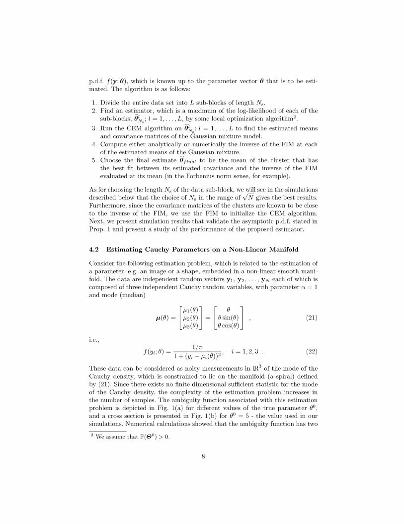
The vector means are known a-priori to lie in the rectangle Θ = {[0, 3]× [0, 3]}.Typical sensor data, generated according to the above model (23) are presentedin Fig. 4. The two circles correspond to the two components.

Each sensor uses the following algorithm to find an estimate. A point isgenerated randomly, according to a uniform distribution on the given rectangleΘ. Then this point is used as the starting point of a local search for a maximumof the log-likelihood function of the measurement. In our simulation, we usedthe Matlab routine ’fminsearch’ which applies the Nelder-Mead algorithm to

12

−0.5 0 0.5 1 1.5 2 2.5 3 3.5−0.5

0

0.5

1

1.5

2

2.5

3

3.5

Fig. 4. Measured data for a single sensor.

maximize the local log-likelihood function LN (Y;θ) with respect to the unknownparameters θ. Denote the estimate from the l’th sensor by θ̂l

N .We have found that the ambiguity function has two maxima in Θ. One

maximum is at the true parameters vector θ0 and the second maximum

θ1 =

2.050.951.081.92

(29)

corresponds to the reversed model, i.e., switching between the two components.Therefore, the estimates θ̂l

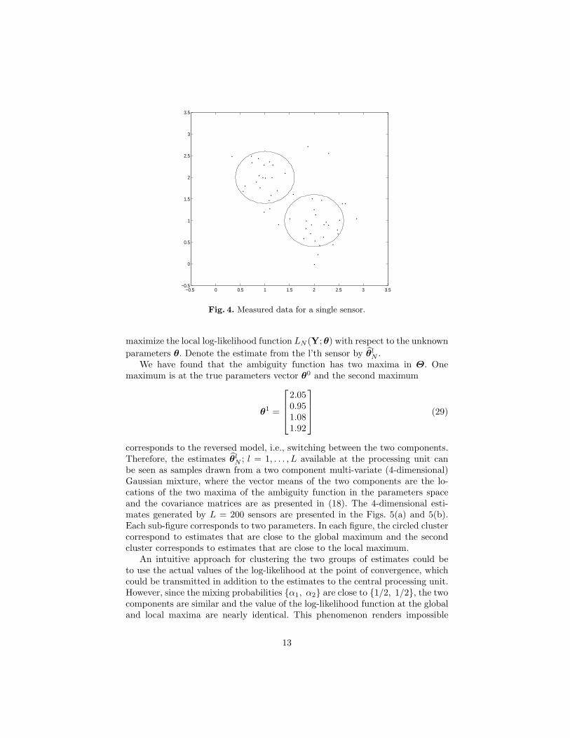
N ; l = 1, . . . , L available at the processing unit canbe seen as samples drawn from a two component multi-variate (4-dimensional)Gaussian mixture, where the vector means of the two components are the lo-cations of the two maxima of the ambiguity function in the parameters spaceand the covariance matrices are as presented in (18). The 4-dimensional esti-mates generated by L = 200 sensors are presented in the Figs. 5(a) and 5(b).Each sub-figure corresponds to two parameters. In each figure, the circled clustercorrespond to estimates that are close to the global maximum and the secondcluster corresponds to estimates that are close to the local maximum.

An intuitive approach for clustering the two groups of estimates could beto use the actual values of the log-likelihood at the point of convergence, whichcould be transmitted in addition to the estimates to the central processing unit.However, since the mixing probabilities {α1, α2} are close to {1/2, 1/2}, the twocomponents are similar and the value of the log-likelihood function at the globaland local maxima are nearly identical. This phenomenon renders impossible

13

0.6 0.8 1 1.2 1.4 1.6 1.8 2 2.2 2.40.6

0.8

1

1.2

1.4

1.6

1.8

2

2.2

µ11

µ 12

0.6 0.8 1 1.2 1.4 1.6 1.8 2 2.2 2.40.6

0.8

1

1.2

1.4

1.6

1.8

2

2.2

µ21

µ 22

Fig. 5. Estimates θ̂lN ; l = 1, . . . , L generated by L = 200 sensors.

75 80 85 90 95 100 1050

5

10

15

20

25

30

Negative log−likelihood function values

Num

ber

of o

ccur

renc

es

Fig. 6. Histogram of the log-likelihood function values ln f(Y; θ̂lN ); l = 1, . . . , L ob-

tained from estimates θ̂lN ; l = 1, . . . , L generated by L = 200 sensors.

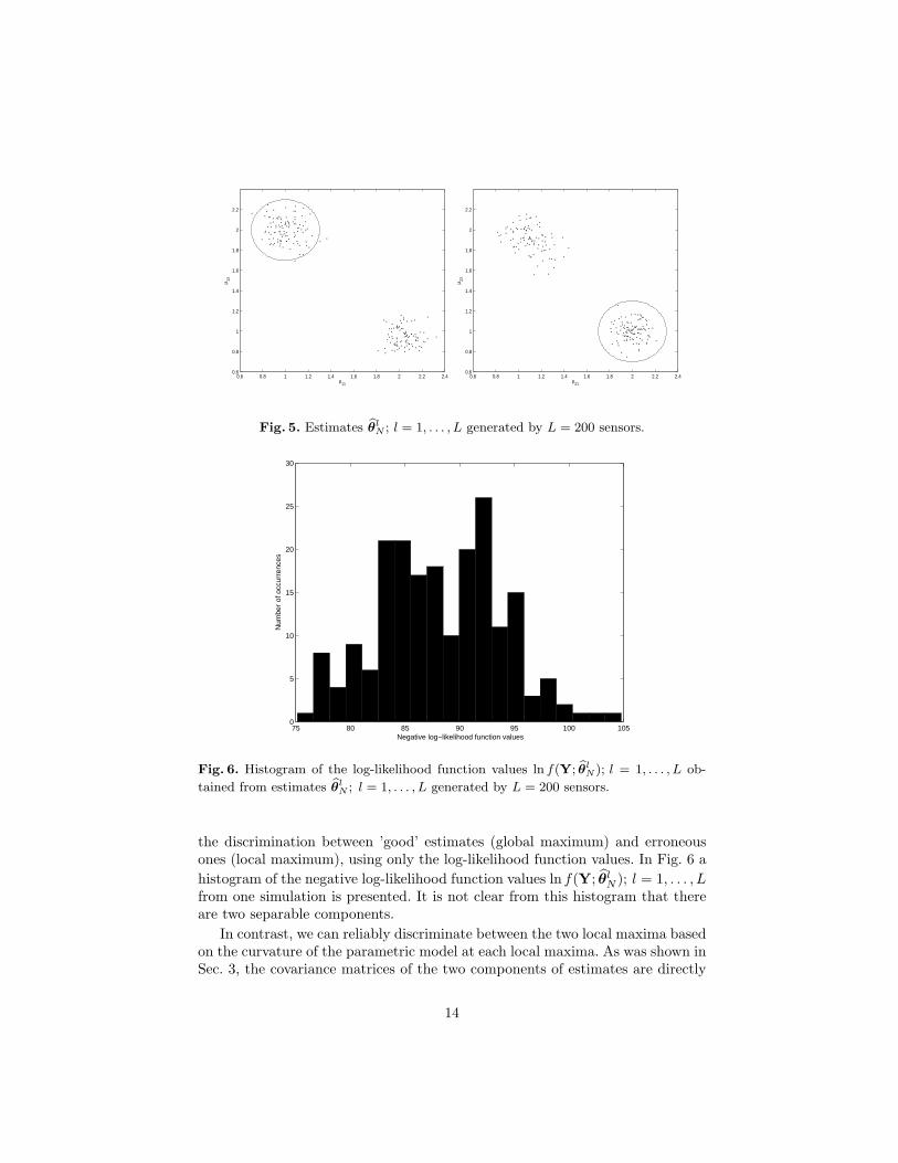
the discrimination between ’good’ estimates (global maximum) and erroneousones (local maximum), using only the log-likelihood function values. In Fig. 6 ahistogram of the negative log-likelihood function values ln f(Y; θ̂l

N ); l = 1, . . . , Lfrom one simulation is presented. It is not clear from this histogram that thereare two separable components.

In contrast, we can reliably discriminate between the two local maxima basedon the curvature of the parametric model at each local maxima. As was shown inSec. 3, the covariance matrices of the two components of estimates are directly

14

related to the curvature of the ambiguity function at the two maxima, and atthe global maximum equal the inverse of the FIM. Therefore, the algorithmproposed in Sec. 4.1 can be applied.

First the number of components, the mean vectors and the covariance ma-trices, of the estimates are estimated using the CEM algorithm. The estimatedmean vectors serve as candidates for the final estimate and the estimated covari-ance matrices provides the means to find the component that corresponds to theglobal maximum. More explicitly, for each component the distance between theestimated covariance and the inverse of the FIM calculated at the point of themean is computed. In our simulation, the Frobenius norm of the difference ma-trix was used as the distance measure. Finally, the mean of the component withthe smallest norm is chosen as the final estimate. Since the 4 × 4 dimensionalFIM cannot be computed analytically, it is computed by numerical integrationand then inverted. The kl entry of the FIM is found by numerically calculatingthe following integral

FIMkl =∫ ∞

−∞

∂ log f(y;θ)∂θk

∂ log f(y;θ)∂θl

f(y;θ)dy , (30)

where the estimated mean of the candidate component is plugged-in for theunknown parameters.

The algorithm was tested in the above setting for several possible numbersof sensors L in order to evaluate two aspects of its performance. The first isthe probability of detecting the global maximum. The second is the small-scaleestimation errors when the global maximum is detected correctly. The algorithmwas run 100 times for L = 50, 100, 150 and 200 sensors. In the case of L = 50sensors, there were 6 cases of erroneous decisions. For systems of 100, 150, and200 sensors there was 100 percent success, i.e. the algorithm always detectedthe correct maximum. The fact that the estimated covariance matrix of the twocomponents is small, which is usually the case when the number of samples ateach sensor is sufficiently large, contributed to the success of the CEM stage.The small-scale estimation errors in cases where the global maximum was de-tected correctly, were compared to the performance of a clairvoyant estimatorwhich knows which local estimates are close to the global max. This clairvoyantestimator averages only those estimates that close to the global maximum. Theperformances of the CEM estimator and the clairvoyant estimator are identical.

5 Concluding Remarks

The work presented in this paper is closely related to the work of White [4] onmisspecified models and to the work of Gan and Jiang [5] on the problem of localmaxima. Given a ML estimate, White proposed a test to detect a misspecifiedmodel. Given a local maximizer of the log-likelihood function, Gan and Jiangoffered the same test in order to detect a scenario of convergence to a localmaximum. This test is based on the observation that the two ways to estimate theFIM from the data given the estimated parameters, i.e., the Hessian form and the

15

outer product form, converge to the same value in the case of a global maximumin a correctly specified model. The test statistic, which is the difference betweenthose two estimators of the FIM, was shown to be asymptotically Gaussiandistributed. However, as mentioned in [5], the convergence of the test statisticto its asymptotic distribution is slow and the test suffers from over rejectionin a moderate number of samples. Therefore, this test could not be used todetermine whether or not the sub-estimates of the algorithm proposed in Sec. 4.1are related to a global maximum. Furthermore, this test requires access to thedata and therefore, could not be used in the estimates fusion problem, discussedin Sec. 4.3.

In contrast, the present paper considers cases in which the complete data aredivided into sub-blocks, either due to computational burden or due to the systemdesign. This data partitioning gives direct access to the estimated covariancematrix of the sub-estimates, which can then be compared to the calculated FIM.This procedure has considerably better performance and does not require re-processing the complete data.

6 Acknowledgement

This work was partially supported by a Dept. of EECS at the University ofMichigan Fellowship and DARPA-MURI Grant Number DAAD19-02-1-0262.

References

1. R. A. Fisher. On the mathematical foundation of theoretical statistics. Phil. Trans.Roy. Soc. London, 222:309–368, 1922.

2. P.J. Huber. Robust Statistics. John Wiley & Sons, 1981.3. P.J. Huber. The behavior of maximum likelihood estimates under nonstandard

conditions. Proceedings of the Fifth Berkeley Symposium in Mathematical Statisticsand Probability, 1967.

4. H. White. Maximum likelihood estimation of misspecified models. Econometrica,50(1):1–26, Jan 1982.

5. L. Gan and J. Jiang. A test for global maximum. Journal of the American Statis-tical Association, 94(447):847–854, Sep 1999.

6. A.K. Jain, R. Duin, and J. Mao. Statistical pattern recognition: A review. IEEETrans. Pattern Analysis and Machine Intelligence, 22(1):4–38, Jan 2000.

7. M.A.T. Figueiredo and A.K. Jain. Unsupervised learning of finite mixute models.IEEE Trans on Pattern Anal and Machine Intelligence, 24:381–396, March 2002.

8. A.P. Dempster, N.M. Laird, and D.B. Rubin. Maximum likelihood from incompletedata using the em algorithm. Ann. Roy. Statist. Soc., 39:1–38, Dec 1977.

9. A. Wald. Note on the consistency of the maximum likelihood estimate. Annals ofMathematical Statistics, 60:595–603, Dec 1949.

10. S.M. Kay. Fundamentals of Statistical Signal Processing - Estimation Theory.Prentice Hall, 1993.

11. P.J. Bickel and K.A. Doksum. Mathematical Statistics. Holden-Day, San Francisco,1977.

16