asymptotic behavior of underlying nt paths in interior point...

Asymptotic Behavior of Underlying NT Paths in Interior Point

Method for Monotone Semidefinite Linear Complementarity

Problems

Chee-Khian Sim1 2

Communicated by F. Potra

1This work was partially supported by a startup grant from The Hong Kong Polytechnic University. Part of

this research was done while the author is a research fellow at the Logistics Institute - Asia Pacific, Singapore,

and at the NUS Business School. The author is grateful to Prof. Paul Tseng for starting him on the proof of

Proposition 3.2, and in getting Example 3.1.2Department of Applied Mathematics, The Hong Kong Polytechnic University, Hung Hom, Kowloon, Hong

Kong. Email: [email protected]

This is the Pre-Published Version.

Abstract

An interior point method (IPM) defines a search direction at each interior point of the feasible region.

These search directions form a direction field, which in turn gives rise to a system of ordinary differential

equations (ODEs). Thus, it is natural to define the underlying paths of the IPM as solutions of the

system of ODEs. In [32], these off-central paths are shown to be well-defined analytic curves and any

of their accumulation points is a solution to the given monotone semidefinite linear complementarity

problem (SDLCP). In [32]-[34], the asymptotic behavior of off-central paths corresponding to the HKM

direction is studied. In particular, in [32], the authors study the asymptotic behavior of these paths

for a simple example, while, in [33,34], the asymptotic behavior of these paths for a general SDLCP

is studied. In this paper, we study off-central paths corresponding to another well-known direction,

the Nesterov-Todd (NT) direction. Again, we give necessary and sufficient conditions for these off-

central paths to be analytic w.r.t.√

µ and then w.r.t. µ, at solutions of a general SDLCP. Also, as in

[32], we present off-central path examples using the same SDP, whose first derivatives are likely to be

unbounded as they approach the solution of the SDP. We work under the assumption that the given

SDLCP satisfies a strict complementarity condition.

Keywords: Semidefinite linear complementarity problem; Interior point methods; NT direction; Local

convergence; Ordinary differential equations

AMS Subject Classification: 90C51; 90C22; 34C05

1 Introduction.

The notion of a central path is introduced by Sonnevend [35] in 1985 to interior point methods (IPMs).

Since then, researchers realize that an IPM is actually a homotopy method following underlying paths

and that many remarkable properties of an IPM are attributed to the nice geometry of these paths.

Readers who are interested to know more about basic geometry of these paths may refer to [2].

An important role the underlying paths play in the study of IPMs is to show its fast local conver-

gence. The classical proof of local convergence of an iterative method, such as the Newton’s method,

for finding the solution of a system of equations relies on the nonsingularity of the Jacobian matrix.

However, the Jacobian matrix of the equation system, defining the search direction in an IPM, may be

singular at an optimal solution. Thus, the traditional approach of local convergence analysis does not

work for IPM. Study of underlying paths, which mimic the behavior of iterates generated by an interior

point algorithm, especially when the iterates are close together at a solution of the given problem, pro-

vides an alternative approach. Fast local convergence of IPMs has been successfully proved by relating

it to the boundedness of derivatives of the underlying paths in [27,38,42,43]. See also [36,37]. Superlin-

ear convergence of IPMs for linear complementarity problem (LCP) is proved in [18,19,20,14,6,24] by

explicitly using the analyticity of off-central path. Also, [10,9,21,22,23] contain results about superlinear

convergence of IPMs for SDP.

Study of fast local convergence is particularly important for the class of monotone semidefinite

linear complementarity problems (SDLCPs), with the class of semidefinite programs (SDPs) as a special

case, because, in contrast to a monotone linear complementarity problem (LCP), the exact solution of

a SDLCP cannot be obtained from an approximate solution by determining a complementary basis.

The analysis for SDP, and hence for SDLCP, is considered to be more difficult than that for linear

programming (LP). This arises mainly due to the difficulty in maintaining symmetry in the linearized

complementarity [44]. Researchers working in the IPM area have proposed ways to overcome this

drawback, which result in different symmetrized search directions, along which iterates generated by

interior point algorithms move [1,7,13,28,29,30,31,41]. Among these search directions, the AHO, HKM

and NT directions are more commonly used.

There are various ways in which the underlying paths, using these different search directions, for

SDLCPs are defined in literature [3,15,17,26,32,40]. Paths arising from different search directions are

likely to behave differently from each other. In [32], a new definition of the underlying paths of IPMs

for SDLCPs, using ordinary differential equations (ODEs), is proposed. The motivation for defining

paths in this way is to relate these paths to the vector field of search directions of an IPM. In [32]-

[34], the behavior of these off-central paths, corresponding to the HKM direction, near solutions of a

1

SDLCP is investigated. It is found that, for off-central paths corresponding to the HKM direction,

their asymptotic behavior [32] suggests that superlinear convergence of iterates, generated by a generic

interior point algorithm using the HKM direction, may not be guaranteed. This contrasts with that for

interior point algorithms using the AHO direction, where it has been shown that superlinear convergence

of iterates, generated by a generic interior point algorithm (which does not, say, perform “narrowing” of

the neighborhood), is possible [1,12,16,17,25,26]. It is interesting to investigate the asymptotic behavior

of off-central paths corresponding to another well-known direction, the so-called NT direction [30,31],

to see whether they behave like that corresponding to the AHO direction or that corresponding to the

HKM direction.

In this paper, we use our definition of paths for SDLCPs [32] to study the asymptotic behavior of

SDLCP paths, corresponding to the NT direction. To the author’s knowledge, this study is the first to

study off-central paths corresponding to the NT direction. In Section 2, through the same simple SDP

example that we used in [32], we show the behavior of a few off-central paths as they approach the

unique solution of the SDP. We show graphically that except for the central path, the first derivatives

of all the other paths are likely to be unbounded as these paths approach the unique solution of the

SDP. In Section 3, considering a general SDLCP, we give necessary and sufficient conditions for an

off-central path, corresponding to the NT direction, to be analytic in the limit, w.r.t.√

µ and then

w.r.t. µ. Here, µ is related to the variable in the primal space and the variable in the dual space for a

SDP (see Remark 2.1). Finally, we give some concluding remarks in Section 4.

1.1 Notations and Common Definitions.

The space of symmetric n×n matrices is denoted by Sn. Given matrices X and Y in <p×q, the standard

inner product is defined by X • Y ≡ Tr(XT Y ), where Tr(·) denotes the trace of a matrix. If X ∈ Sn

is positive semidefinite (resp., positive definite), we write X º 0 (resp., X Â 0). The cone of positive

semidefinite (resp., positive definite) symmetric matrices is denoted by Sn+ (resp., Sn

++). Either the

identity matrix or operator will be denoted by I. Eij ∈ <n×n is a square matrix with 1 at its (i, j)

entry and the rest of entries equal to zero. ‖ · ‖ for a vector in <n refers to its Euclidean norm, and for

a matrix in <p×q, it refers to its Frobenius norm.

For a matrix X ∈ <p×q, we denote its component at the ith row and jth column by Xij . Also,

Xi· denotes the ith row of X, and X·j the jth column of X. In case X is partitioned into blocks of

submatrices, then Xij refers to the submatrix in the corresponding (i, j) position.

Given square matrices Ai ∈ <ni×ni , i = 1, . . . , m, Diag(A1, . . . , Am) is a square matrix with Ai as

its diagonal blocks arranged in accordance to the way they are lined up in Diag(A1, . . . , Am). All the

2

other entries in Diag(A1, . . . , Am) are taken to be zero.

Given functions f : Ω −→ E and g : Ω −→ <++, where Ω is an arbitrary set and E is a

normed vector space, and a subset Ω ⊆ Ω, we write f(w) = O(g(w)) for all w ∈ Ω to mean that

‖f(w)‖ ≤ Mg(w) for all w ∈ Ω, where M > 0 is a positive constant. Suppose we have E = Sn. Then

we write f(w) = Θ(g(w)) if for all w ∈ Ω, f(w) ∈ Sn++, f(w) = O(g(w)) and f(w)−1 = O(1/g(w)).

What the subset Ω is should be clear from the context. Usually, Ω = (0, w) for a small w > 0.

A function f = (f1, . . . , fm) from an open subset O of <k to <m is analytic at a point x =

(x1, . . . , xk) ∈ O iff each fi, i = 1, . . . , m, can be written as a convergent power series expansion about

x in an open neighborhood of x. Furthermore, if x0 ∈ <k is on the boundary of O, we say f is analytic

at x0 (or can be extended analytically to x0), and we let f(x0) = limx→x0 f(x), iff there exists an

analytic function g, which is analytic at x0 and coincides with f wherever both are defined.

The above also applies if a component xj of x = (x1, . . . , xk) is a symmetric matrix, instead of a

number, in which case, we consider xj to lie in an Euclidean space of appropriate dimension. If the

range of f is in the space of (symmetric) matrices, we also view the space as an appropriate Euclidean

space, when considering analyticity, so that the above applies.

2 Definition of an Off-central Path and an Investigation on NT

Paths for an Example.

Let us consider the following SDLCP:

XY = 0, (1)

A(X) + B(Y ) = q, (2)

X, Y ∈ Sn+, (3)

where A,B : Sn −→ <n are linear operators mapping Sn to the space <n, where n := n(n+1)/2. Hence

A and B have the form A(X) = (A1 • X, . . . , An • X)T , respectively, B(Y ) = (B1 • Y, . . . , Bn • Y )T ,

where Ai, Bi ∈ Sn for all i = 1, . . . , n. Also, q ∈ <n.

We have the following assumptions on the SDLCP throughout the paper:

Assumption 2.1 (a) SDLCP is monotone, i.e., A(X) + B(Y ) = 0 for X, Y ∈ Sn ⇒ X • Y ≥ 0.

(b) There exist X1, Y 1 Â 0, such that A(X1) + B(Y 1) = q.

(c) A(X) + B(Y ) : X, Y ∈ Sn = <n.

3

Assumption 2.1(a)-(c) are basic assumptions used in the literature when SDLCP is studied in the

context of IPM.

Let us now define the off-central path for SDLCP passing through a point (X0, Y 0), X0, Y 0 Â 0,

satisfying A(X) + B(Y ) = q.

Definition 2.1 The solution (X(µ), Y (µ)), X(µ), Y (µ) Â 0, to

HP (XY ′ + X ′Y ) =1µ

HP (XY ), (4)

A(X ′) + B(Y ′) = 0, (5)

where µ > 0, with the initial condition (X(1), Y (1)) = (X0, Y 0), X0, Y 0 Â 0, is the off-central path

for SDLCP, corresponding to P , passing through (X0, Y 0). Here HP (U) := 12 (PUP−1 + (PUP−1)T ),

and P ∈ <n×n is an invertible matrix.

Assuming P be an analytic function of X, Y and PXY P−1 be always symmetric (such P include

the well-known directions like the HKM, and its dual, and NT directions), it is proved in [32] that the

above is well-defined, and (X(µ), Y (µ)) is unique, analytic over µ ∈ (0,∞). The motivation for defining

an off-central path as in Definition 2.1 is also given in [32].

Remark 2.1 The central path (Xc(µ), Yc(µ)) for SDLCP, which satisfies Xc(µ)Yc(µ) = µI, is a special,

but important, example of an off-central path for SDLCP. When µ = 1, it satisfies Tr(Xc(1)Yc(1)) = n.

Therefore, we also require the initial data (X0, Y 0) when µ = 1 in (4)-(5) to satisfy Tr(X0Y 0) = n. In

this case, using (4), it is easy to see that the parameter µ in the ODE system (4)-(5) actually represents

the duality gap, X(µ) • Y (µ), at the point (X(µ), Y (µ)) on the path.

Let us now consider a SDP example as follows:

(P) min

0 0

0 1

•X

subject to

2 0

0 0

•X = 2,

0 −1

−1 2

•X = 0, X ∈ S2

+

and

(D) max 2v1

subject to v1

2 0

0 0

+ v2

0 −1

−1 2

+ Y =

0 0

0 1

, Y ∈ S2

+.

This example, which first appeared in [11], has all the nice properties (e.g. primal and dual

nondegeneracy, strict complementarity, e.t.c.) for a SDP. The example is also used in [?] to analyze the

asymptotic behavior of its off-central paths corresponding to the HKM direction.

4

It has an unique solution,

1 0

0 0

,

0 0

0 1

, which satisfies strict complementarity and

nondegeneracy.

Written as a SDLCP, the above example can be expressed as

XY = 0

Asvec(X) + Bsvec(Y ) = q

X, Y ∈ S2+,

where A =

2 0 0

0 0 0

0 −√2 2

, B =

0 0 0

0√

2 1

0 0 0

and q =

2

1

0

. Note that A and B are the

corresponding matrix representation of the linear operator A and B respectively in (2).

In [32], off-central paths for the example are analyzed. The off-central paths analyzed correspond to

the dual HKM direction, which are obtained by setting P = Y 1/2 in (4). It is shown analytically in [32]

that unless an off-central path satisfies certain algebraic condition, its first derivatives are unbounded

in the limit as the path approaches the unique solution of the example. In this section, we consider

off-central paths for the same SDP example, but corresponding to the NT direction, where P in (4) is

such that PT P = W−1, W is a symmetric, positive definite matrix with WY W = X.

Although it is known that one can express W in terms of X and Y , it is still difficult to write

down explicitly each entry of W in terms of that of X and Y for the example, even if these matrices

are only of size two. We are therefore unable to further analyze the asymptotic behavior of these paths

analytically, like the (dual) HKM case in [32]. As an alternative, we have written Matlab codes to study

the behavior of the first derivatives of various off-central paths corresponding to the NT direction, for

the example.

Using Tr(X0Y 0) = 2 and (5), we have the off-central path for the example, (X(µ), Y (µ)), passing

through (X0, Y 0) = (X(1), Y (1)), is of the form

X(µ) =

1 2µ− y1(µ)

2µ− y1(µ) 2µ− y1(µ)

and Y(µ) =

y1(µ) y2(µ)

y2(µ) 1− 2y2(µ)

.

The central path for the example is given by

Xc(µ) =

1 2µ− yc

1(µ)

2µ− yc1(µ) 2µ− yc

1(µ)

and Yc(µ) =

yc

1(µ) yc2(µ)

yc2(µ) 1− 2yc

2(µ)

,

where yc2(µ) = −yc

1(µ) and

yc1(µ) =

2µ√1 + 4µ2 + 1− 2µ

. (6)

5

In the below plots, X0 are all set to be equal to Xc(1), while Y 0 are varied by varying y02 = y2(1),

keeping y01 = y1(1) equal to yc

1(1) = 2√5−1

.

2 2.5 3 3.5 4 4.5 5 5.5

x 10−10

300

310

320

330

340

350

360

µ

Su

m o

f n

orm

sq

ua

red

of firs

t d

eriva

tive

s

y20=0.25

2 2.5 3 3.5 4 4.5 5 5.5

x 10−10

1150

1200

1250

1300

1350

1400

1450

1500

µ

Su

m o

f n

orm

sq

ua

red

of firs

t d

eriva

tive

s

y20=0

2 2.5 3 3.5 4 4.5 5 5.5

x 10−10

5000

5500

6000

6500

7000

7500

8000

µ

Su

m o

f n

orm

sq

ua

red

of firs

t d

eriva

tive

s

y20=−0.6

1 1.5 2 2.5 3 3.5

x 10−5

1.99

2

2.01

2.02

2.03

2.04

2.05

2.06

2.07

2.08

2.09

µ

Su

m o

f n

orm

sq

ua

red

of firs

t d

eriva

tive

s

y20=−1.6

1 1.5 2 2.5 3 3.5

x 10−5

3.1623

3.1623

3.1623

3.1623

3.1623

3.1623

3.1623

3.1623

3.1623

3.1624

3.1624

µ

Su

m o

f n

orm

sq

ua

red

of firs

t d

eriva

tive

s

Central Path

6

2 2.5 3 3.5 4 4.5 5 5.5

x 10−10

450

500

550

600

650

700

750

µ

Su

m o

f n

orm

sq

ua

red

of firs

t d

eriva

tive

s

y20=−1.6

2 2.5 3 3.5 4 4.5 5 5.5

x 10−10

3.1623

3.1623

3.1623

3.1623

3.1623

3.1623

3.1623

3.1623

3.1623

µ

Su

m o

f n

orm

sq

ua

red

of firs

t d

eriva

tive

s

Central Path

As observed from these plots, we see that except for the case when the off-central path is actually

the central path, the sums of norm squared of first derivatives1 of the given paths get larger as µ

approaches zero. The first three plots are for paths that are initiated relatively far from the central

path, while the fourth and sixth plots are for the same off-cental path that is initiated near to the

central path. Comparison between the fourth and fifth plot shows that for this off-central path with

y02 = −1.6, for the same range of µ, the sum of norm squared of its derivatives starts to increase while

that of the central path remains stable. For the case of the central path, one can observe that its sum

of first derivatives’ norm squared is approaching 3.162 . . . as µ approaches zero (seventh plot), which

should be the case, as can be verified using yc2(µ) = −yc

1(µ) and (6).

Hence, from these graphical examples, they indicate the possibility that unless the off-central paths

corresponding to the NT direction, for the example, satisfy certain condition, their first derivatives are

likely to be unbounded as µ tends to zero.

3 Asymptotic Analyticity Behavior of NT Paths for a general

SDLCP.

Based on what is observed of the first derivatives of off-central paths for the SDP example in the above

section, it suggests that off-central paths corresponding to the NT direction are in general not analytic

at solutions of a SDLCP. In this section, we study the conditions that are required to ensure analyticity

of paths corresponding to the NT direction, for a general SDLCP. We investigate the asymptotic

analyticity of an off-central path, corresponding to the NT direction, first w.r.t.√

µ and then w.r.t.

1Sum of norm squared of first derivatives here stands for√‖X′(µ)‖2 + ‖Y ′(µ)‖2.

7

µ. By studying the conditions which ensure asymptotic analyticity of paths, one can hope to ensure

that iterates generated by interior point algorithms are guaranteed to converge superlinearly as they

approach a solution of a given SDLCP.

We require an additional assumption, besides Assumption 2.1, to carry out the analysis.

Assumption 3.1 There exists a strictly complementary solution, (X∗, Y ∗), to SDLCP (1)-(3).

The analysis of the asymptotic behavior of an off-central path for a general SDLCP is considered

to be difficult without this assumption (Assumption 3.1). However, we note that there have been some

work done in this area for special classes of SDLCP without the assumption. See for example [5].

Let (X∗, Y ∗) be a strictly complementary solution to SDLCP (1)-(3), which exists by Assumption

3.1.

Since X∗ and Y ∗ commute, they are jointly diagonalizable by some orthogonal matrix. So, using

a suitable orthogonal similarity transformation of the matrices in SDLCP (1)-(3), we may assume,

without loss of generality, that

X∗ =

Λ∗11 0

0 0

, Y ∗ =

0 0

0 Λ∗22

,

where Λ∗11 = Diag(λ∗1, . . . , λ∗m) Â 0 and Λ∗22 = Diag(λ∗m+1, . . . , λ

∗n) Â 0. Here λ∗1, . . . , λ

∗n are real

numbers greater than zero.

Hereafter, whenever we partition a matrix S ∈ Sn, we do it in a similar way, i.e., S is always

partitioned as

S11 S12

ST12 S22

, where S11 ∈ Sm, S22 ∈ Sn−m and S12 ∈ <m×(n−m). The same holds for

S ∈ <n×n, which may not necessarily be symmetric.

3.1 Analyticity w.r.t.√

µ.

Let us now analyze the analyticity of off-central paths, corresponding to the NT direction, w.r.t.√

µ.

From now onwards, we may occasionally suppress the dependence of a variable on another variable.

For example, instead of writing X(µ) for the primal part of an off-central path, we simply write X. We

do this only when the dependency is clear from the context, and also for the sake of not cluttering an

expression with too many symbols.

Written in matrix-vector form, the ODE system (4)-(5) can be expressed as:

svec(A1)T svec(B1)T

......

svec(An)T svec(Bn)T

P ⊗s (P−T Y ) (PX)⊗s P−T

svec(X ′)

svec(Y ′)

=

1µ

0

svec(HP (XY ))

, (7)

8

where n = n(n + 1)/2.

Here, the operation ⊗s and the map svec (with inverse smat) are used, whose properties are given

on pp. 775− 776 and the appendix of [39].

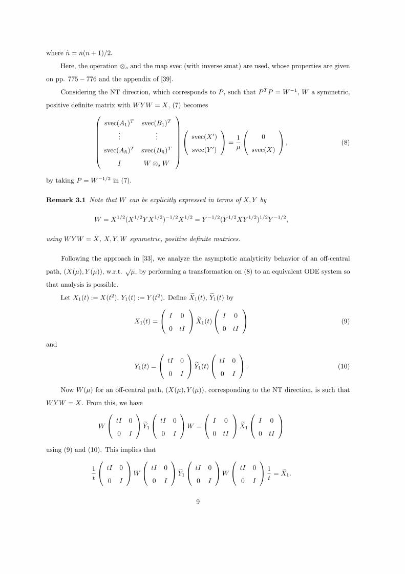
Considering the NT direction, which corresponds to P , such that PT P = W−1, W a symmetric,

positive definite matrix with WY W = X, (7) becomes

svec(A1)T svec(B1)T

......

svec(An)T svec(Bn)T

I W ⊗s W

svec(X ′)

svec(Y ′)

=

1µ

0

svec(X)

, (8)

by taking P = W−1/2 in (7).

Remark 3.1 Note that W can be explicitly expressed in terms of X, Y by

W = X1/2(X1/2Y X1/2)−1/2X1/2 = Y −1/2(Y 1/2XY 1/2)1/2Y −1/2,

using WY W = X, X, Y,W symmetric, positive definite matrices.

Following the approach in [33], we analyze the asymptotic analyticity behavior of an off-central

path, (X(µ), Y (µ)), w.r.t.√

µ, by performing a transformation on (8) to an equivalent ODE system so

that analysis is possible.

Let X1(t) := X(t2), Y1(t) := Y (t2). Define X1(t), Y1(t) by

X1(t) =

I 0

0 tI

X1(t)

I 0

0 tI

(9)

and

Y1(t) =

tI 0

0 I

Y1(t)

tI 0

0 I

. (10)

Now W (µ) for an off-central path, (X(µ), Y (µ)), corresponding to the NT direction, is such that

WY W = X. From this, we have

W

tI 0

0 I

Y1

tI 0

0 I

W =

I 0

0 tI

X1

I 0

0 tI

using (9) and (10). This implies that

1t

tI 0

0 I

W

tI 0

0 I

Y1

tI 0

0 I

W

tI 0

0 I

1

t= X1.

9

Define

W1(t) :=1t

tI 0

0 I

W (t2)

tI 0

0 I

. (11)

Remark 3.2 X1(t), Y1(t) and W1(t) (of an off-central path) given above in (9)-(11) satisfy W1Y1W1 =

X1. Hence, we can write

W1 = X1/21 (X1/2

1 Y1X1/21 )−1/2X

1/21 (12)

by Remark 3.1. Therefore, W1 is an analytic function of X1, Y1, and for (X1(t), Y1(t)) corresponding

to the off-central path (X(µ), Y (µ)), W1(t) is an analytic function of t. Also, by (9), and that

X1(t) =

Θ(1) O(t)

O(t) Θ(t2)

,

we have X1(t) is symmetric, positive definite in the limit as t approaches zero. Similar property holds

for Y1(t). Using (12), W1(t) is hence symmetric, positive definite in the limit as t approaches zero.

Let us now reformulate (8) in terms of X1(t), Y1(t), W1(t), their derivatives and t, in order to

analyze the asymptotic analyticity behavior of (X1(t), Y1(t)) = (X(t2), Y (t2)), as t approaches zero.

From (8), we have

svec(X ′) + (W ⊗s W )svec(Y ′) =1µ

svec(X).

Expressing the above in terms of X1(t), Y1(t), W1(t), their derivatives and t(=√

µ), we obtain

svec(X ′1) + (W1 ⊗s W1)svec(Y ′

1)

=1t

I 0

0 −I

⊗s I

svec(X1)− 1

t(W1 ⊗s W1)

I 0

0 −I

⊗s I

svec(Y1).

(13)

Following [33],

svec(A1)T

...

svec(An)T

svec(X ′) +

svec(B1)T

...

svec(Bn)T

svec(Y ′) = 0

from (8) can be expressed as

A(t)svec(X ′1) + B(t)svec(Y ′

1) = −G(t)svec(X1)−H(t)svec(Y1), (14)

10

where

A(t)k· :=

svec

(Ak)11 t(Ak)12

t(Ak)T12 t2(Ak)22

T

for 1 ≤ k ≤ i1

svec

0 (Ak)12

(Ak)T12 t(Ak)22

T

for i1 + 1 ≤ k ≤ i1 + i2

svec

0 0

0 (Ak)22

T

for i1 + i2 + 1 ≤ k ≤ n

, (15)

B(t)k· :=

svec

t2(Bk)11 t(Bk)12

t(Bk)T12 (Bk)22

T

for 1 ≤ k ≤ i1

svec

t(Bk)11 (Bk)12

(Bk)T12 0

T

for i1 + 1 ≤ k ≤ i1 + i2

svec

(Bk)11 0

0 0

T

for i1 + i2 + 1 ≤ k ≤ n

, (16)

G(t)k· :=

svec

0 (Ak)12

(Ak)T12 2t(Ak)22

T

for 1 ≤ k ≤ i1

svec

0 0

0 (Ak)22

T

for i1 + 1 ≤ k ≤ i1 + i2

0 for i1 + i2 + 1 ≤ k ≤ n

, (17)

and

H(t)k· :=

svec

2t(Bk)11 (Bk)12

(Bk)T12 0

T

for 1 ≤ k ≤ i1

svec

(Bk)11 0

0 0

T

for i1 + 1 ≤ k ≤ i1 + i2

0 for i1 + i2 + 1 ≤ k ≤ n

, (18)

for some fixed i1, i2.

Details on how A(t),B(t),G(t) and H(t) are derived can be obtained from [33].

Combining (13) and (14), we have that (X1(t), Y1(t)), corresponding to the off-central path

11

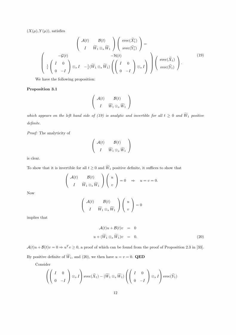
(X(µ), Y (µ)), satisfies A(t) B(t)

I W1 ⊗s W1

svec(X ′

1)

svec(Y ′1)

=

−G(t) −H(t)

1t

I 0

0 −I

⊗s I − 1

t (W1 ⊗s W1)

I 0

0 −I

⊗s I

svec(X1)

svec(Y1)

.

(19)

We have the following proposition:

Proposition 3.1 A(t) B(t)

I W1 ⊗s W1

which appears on the left hand side of (19) is analytic and invertible for all t ≥ 0 and W1 positive

definite.

Proof: The analyticity of A(t) B(t)

I W1 ⊗s W1

is clear.

To show that it is invertible for all t ≥ 0 and W1 positive definite, it suffices to show that A(t) B(t)

I W1 ⊗s W1

u

v

= 0 ⇒ u = v = 0.

Now A(t) B(t)

I W1 ⊗s W1

u

v

= 0

implies that

A(t)u + B(t)v = 0

u + (W1 ⊗s W1)v = 0. (20)

A(t)u + B(t)v = 0 ⇒ uT v ≥ 0, a proof of which can be found from the proof of Proposition 2.3 in [33].

By positive definite of W1, and (20), we then have u = v = 0. QED

Consider

I 0

0 −I

⊗s I

svec(X1)− (W1 ⊗s W1)

I 0

0 −I

⊗s I

svec(Y1)

12

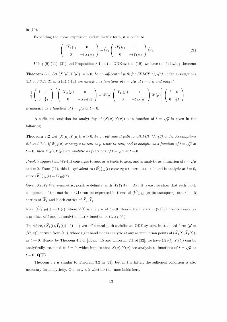
in (19).

Expanding the above expression and in matrix form, it is equal to (X1)11 0

0 −(X1)22

− W1

(Y1)11 0

0 −(Y1)22

W1. (21)

Using (9)-(11), (21) and Proposition 3.1 on the ODE system (19), we have the following theorem:

Theorem 3.1 Let (X(µ), Y (µ)), µ > 0, be an off-central path for SDLCP (1)-(3) under Assumptions

2.1 and 3.1. Then X(µ), Y (µ) are analytic as functions of t =√

µ at t = 0 if and only if

1t

I 0

0 1t I

X11(µ) 0

0 −X22(µ)

−W (µ)

Y11(µ) 0

0 −Y22(µ)

W (µ)

I 0

0 1t I

is analytic as a function of t =√

µ at t = 0.

A sufficient condition for analyticity of (X(µ), Y (µ)) as a function of t =√

µ is given in the

following:


2.1 and 3.1. If W12(µ) converges to zero as µ tends to zero, and is analytic as a function of t =√

µ at

t = 0, then X(µ), Y (µ) are analytic as functions of t =√

µ at t = 0.

Proof. Suppose that W12(µ) converges to zero as µ tends to zero, and is analytic as a function of t =√

µ

at t = 0. From (11), this is equivalent to (W1)12(t) converges to zero as t → 0, and is analytic at t = 0,

since (W1)12(t) = W12(t2).

Given X1, Y1, W1, symmetric, positive definite, with W1Y1W1 = X1. It is easy to show that each block

component of the matrix in (21) can be expressed in terms of (W1)12 (or its transpose), other block

entries of W1 and block entries of X1, Y1.

Now, (W1)12(t) = tV (t), where V (t) is analytic at t = 0. Hence, the matrix in (21) can be expressed as

a product of t and an analytic matrix function of (t, X1, Y1).

Therefore, (X1(t), Y1(t)) of the given off-central path satisfies an ODE system, in standard form (y′ =

f(t, y)), derived from (19), whose right hand side is analytic at any accumulation points of (X1(t), Y1(t)),

as t → 0. Hence, by Theorem 4.1 of [4], pp. 15 and Theorem 2.1 of [32], we have (X1(t), Y1(t)) can be

analytically extended to t = 0, which implies that X(µ), Y (µ) are analytic as functions of t =√

µ at

t = 0. QED

Theorem 3.2 is similar to Theorem 3.2 in [33], but in the latter, the sufficient condition is also

necessary for analyticity. One may ask whether the same holds here.

13

If (X1(t), Y1(t)) is analytic at t = 0, then clearly, (W1)12(t) is analytic at t = 0. What about the

condition “(W1)12(t) tends to zero as t → 0”? If this condition holds, then the sufficient condition for

asymptotic analyticity of (X1(t), Y1(t)) in the above Theorem 3.2, which is equivalent to “(W1)12(t)

converges to zero as t → 0 and is analytic at t = 0”, is also necessary.

Suppose (X1(t), Y1(t)) derived from an off-central path, (X(µ), Y (µ)), corresponding to the NT

direction is analytic at t = 0. These lead to the following conditions which must be satisfied by

X∗1 = limt→0 X1(t), Y ∗

1 = limt→0 Y1(t), W ∗1 = limt→0 W1(t):

W ∗1 Y ∗

1 W ∗1 = X∗

1 , (22)

W ∗1

(Y ∗

1 )11 0

0 −(Y ∗1 )22

W ∗

1 =

(X∗

1 )11 0

0 −(X∗1 )22

. (23)

Here, X∗1 , Y ∗

1 , W ∗1 are symmetric, positive definite matrices.

Condition (22) is derived from the fact that (X1(t), Y1(t)) is derived from an off-central path

corresponding to the NT direction, while Condition (23) is necessary for (X1(t), Y1(t)) to be analytic

at t = 0.

Also, from the monotonicity assumption of SDLCP (1)-(3), Assumption 2.1(a), we have X∗1 , Y ∗

1

must also satisfy

(X∗1 )12 • (Y ∗

1 )12 ≥ 0. (24)

Does Conditions (22)-(24) suffice to conclude that (W1)12(t) converges to zero as t → 0, that is,

(W ∗1 )12 = 0?

It turns out that in general, using Conditions (22)-(24), we cannot conclude that (W ∗1 )12 = 0. Here

is a counterexample:

Example 3.1 Let

(W ∗1 )12 =

0 0

β 0

, (Y ∗

1 )12 =

0 β1

−β 0

,

(Y ∗1 )11 = (Y ∗

1 )22 = (W ∗1 )11 = (W ∗

1 )22 = I2×2.

Choose β be a small value between 0 and 1, and

β21 = −β4 + β2.

We have X∗1 , Y ∗

1 and W ∗1 defined this way, where X∗

1 = W ∗1 Y ∗

1 W ∗1 , are symmetric, positive definite

matrices satisfying (22)-(24) with (24) being satisfied with equality, while (W ∗1 )12 6= 0.

14

However, under a further restriction on the matrices involved, the conclusion “(W ∗1 )12 = 0” holds,

as shown in the following proposition:

Proposition 3.2 If the upper left hand block of every matrix involved is one dimensional, Conditions

(22)-(24) implies that (W ∗1 )12 = 0.

Proof. By pre-multiplying and post-multiplying Y ∗1 by

(Y ∗

1 )−1/211 0

0 (Y ∗1 )−1/2

22

, (25)

we can assume the diagonal blocks of Y ∗1 to be identity matrices. Also, in order for Conditions (22)-(24)

to hold for the new Y ∗1 , we have to take the new W ∗

1 to be W ∗1 pre- and post-multiplied by the inverse

of the above matrix (25).

With these transformations, if the upper left hand block of every matrix involved is one dimensional,

we have

Y ∗1 =

1 yT

y I

, W ∗

1 =

w11 wT

w (W ∗1 )22

,

where w11 is a scalar and y, w are column vectors.

We are done if we can show that w = 0.

From Conditions (22) and (23), we have

w11wT y + ‖w‖2 = 0, (26)

2wwT + (W ∗1 )22ywT + wyT (W ∗

1 )22 = 0, (27)

w11w = (W ∗1 )22w. (28)

Post-multiplying the equation in (27) by w, we obtain

2‖w‖2w + ‖w‖2(W ∗1 )22y + wyT (W ∗

1 )22w = 0.

Using (28) and then (26) on the above equation, we obtain y = −(W ∗1 )−1

22 w, if we assume w 6= 0.

Using Condition (24), we have

w11wT y + (wT y)2 + w11y

T (W ∗1 )22y + wT (W ∗

1 )22y ≥ 0.

15

Substituting y = −(W ∗1 )−1

22 w derived earlier into the above inequality and using (28), we obtain

‖w‖2(‖w‖2

w211

− 1)≥ 0.

Since we assume w 6= 0, we then have ‖w‖ ≥ w11. But this is a contradiction to the positive definiteness

of W ∗1 . Hence we are done. QED

From Proposition 3.2, we have the following corollary:

Corollary 3.1 Let m = 1 or m = n− 1, that is, a primal optimal solution X∗ to SDLCP (1)-(3) has

rank 1 or n− 1.

Suppose (X(µ), Y (µ)), µ > 0, is an off-central path for SDLCP (1)-(3) under Assumptions 2.1 and 3.1.

Then X(µ), Y (µ) are analytic as functions of t =√

µ at t = 0 if and only if W12(µ) converges to zero

as µ tends to zero, and is analytic as a function of t =√

µ at t = 0.

Remark 3.3 From Example 3.1, we see that for 2 ≤ m ≤ n−2, the sufficient condition in Theorem 3.2

is unlikely to be also necessary for analyticity of an off-central path corresponding to the NT direction,

w.r.t.√

µ, in general.

3.2 Analyticity w.r.t. µ.

Now, let us turn our attention to the analyticity of off-central paths, corresponding to the NT direction,

w.r.t. µ.

To analyze the analyticity of an off-central path, (X(µ), Y (µ)), with respect to µ, a necessary

condition is that X12(µ) = O(µ) and Y12(µ) = O(µ). Hence, we take X12(µ) = O(µ), Y12(µ) = O(µ)

from now onwards. Also, a necessary condition for X(µ), Y (µ) to be analytic at µ = 0 is W12(µ) =

O(√

µ). To see this, we observe that X12(µ) = O(µ), Y12(µ) = O(µ) imply that W12(µ) → 0 as µ → 0.

Also, X(µ), Y (µ) analytic at µ = 0 implies that they are analytic as a function of t =√

µ at t = 0.

That is, X1(t), Y1(t) are analytic at t = 0. Hence, W1(t), in particular, (W1)12(t) = W12(t2) is analytic

at t = 0. Therefore, with W12(µ) → 0 as µ → 0, we have W12(µ) = O(√

µ).

Analyzing analyticity w.r.t. µ involves different transformation on X(µ) and on Y (µ), as compared

to the case, ((9), (10)), of analyticity w.r.t.√

µ, [34].

Following [34], let us define X(µ) and Y (µ) which are related to X(µ), Y (µ) by

X(µ) = X(µ)

I 0

0 µI

(29)

and

Y (µ) =

µI 0

0 I

Y (µ). (30)

16

Since X11(µ) = Θ(1), X12(µ) = O(µ), X22(µ) = Θ(µ), we have X(µ) = O(1). Similarly, we have

Y (µ) = O(1).

From WY W = X which must be satisfied by (X(µ), Y (µ)) - an off-central path corresponding to

the NT direction, we have

W

µI 0

0 I

Y W = X

I 0

0 µI

which implies that

W

√

µI 0

0 1√µI

Y W

√

µI 0

0 1√µI

= X.

Define

W (µ) := W (µ)

√

µI 0

0 1√µI

. (31)

Therefore, we have W Y W = X. Also, X(µ), Y (µ), W (µ) are invertible even in the limit as µ → 0.

Note that accumulation points of W (µ) exist as µ → 0 since W (µ) = O(1). The latter follows from

W11(µ) = O(

1√µ

), W22 = O(

√µ) and W12(µ) = O(

√µ).

Since the “tilde” matrices are in general nonsymmetric, instead of using the operation ⊗s and the

map svec, we consider the operation ⊗ and the map vec (with inverse mat) from now on. Properties of

these can be found for example in Chapter 4 of [8] and the appendix of [39].

From (4) (with P , such that PT P = W−1, W a symmetric, positive definite matrix and WY W =

X), we have

X ′ + WY ′W =1µ

X.

Expressing the latter in terms of X, Y , W , their derivatives and µ, we obtain

vec(X ′) + (WT ⊗ W )vec(Y ′) =1µ

vec

X

I 0

0 0

− W

I 0

0 0

Y W

. (32)

Now, in the wider context when we treat X, Y ∈ <n×n instead of in Sn, let us introduce the

following:

(Eij − Eji) ·X = 0, 1 ≤ i < j ≤ n, (33)

(Eij − Eji) · Y = 0, 1 ≤ i < j ≤ n, (34)

to (2) to form

(A1 B1)

vec(X)

vec(Y )

=

q

0

, (35)

17

where

(A1 B1) =

vec((A1)1) vec((B1)1)...

...

vec((A1)n2+n(n−1)/2) vec((B1)n2+n(n−1)/2)

:=

vec(A1)T vec(B1)T

......

vec(An)T vec(B

n)T

vec(Eij − Eji)T1≤i<j≤n 0

0 vec(Eij − Eji)T1≤i<j≤n

∈ <(n2+n(n−1)/2)×2n2.

Conditions (33), (34) are introduced to ensure that although X, Y belong to <n×n, they are

necessarily symmetric.

From (35), together with (32) (see [34]), we have the following ODE system: A1(µ) B1(µ)

I WT ⊗ W

vec(X ′)

vec(Y ′)

=

1µ

−A1(µ)

0 0

0 I

⊗ I

vec(X)− B1(µ)

I ⊗

I 0

0 0

vec(Y )

vec

X

I 0

0 0

− W

I 0

0 0

Y W

,

(36)

where

A1(µ)k· :=

vec

((A1)k)11 µ((A1)k)12

((A1)k)21 µ((A1)k)22

T

for 1 ≤ k ≤ i′1

vec

0 ((A1)k)12

0 ((A1)k)22

T

for i′1 + 1 ≤ k ≤ n2 + n(n− 1)/2

(37)

and

B1(µ)k· :=

vec

µ((B1)k)11 µ((B1)k)12

((B1)k)21 ((B1)k)22

T

for 1 ≤ k ≤ i′1

vec

((B1)k)11 ((B1)k)12

0 0

T

for i′1 + 1 ≤ k ≤ n2 + n(n− 1)/2

, (38)

for some fixed i′1.

Details on how A1(µ),B1(µ) are derived and their properties can be obtained from [34].

18

The analyticity of the matrix A1(µ) B1(µ)

I WT ⊗ W

,

which appears on the left hand side of (36), in an open neighborhood of (µ, X(µ), Y (µ)), µ > 0, of an

off-central path, and its accumulation points, is given in the following proposition. Analyticity of this

matrix is required to analyze the asymptotic analyticity behavior of paths corresponding to the NT

direction, using ODE system (36) (or (42)).

Before we state and prove the proposition, let us first state a well-known result which will be used

in the proof of the proposition.

Result 3.1 Let A ∈ <p×p and B ∈ <q×q. The equation AX + XB = C has an unique solution

X ∈ <p×q for each C ∈ <p×q if and only if σ(A) ∩ σ(−B) = ∅.Here, σ(A) refers to the set of all eigenvalues of the square matrix A.

The above result can be found for example in Chapter 4 of [8].

Proposition 3.3 There exists an open neighborhood U ⊂ <×<n×n×<n×n of (µ, X(µ), Y (µ)), µ > 0,

of an off-central path, and (0, X∗, Y ∗) corresponding to any accumulation point of the off-central path,

such that for (µ, X, Y ) ∈ U , the matrix A1(µ) B1(µ)

I WT ⊗ W

is analytic at (µ, X, Y ), where W exists, is an analytic function of (X, Y ), and satisfies W Y W = X.

Proof. Consider

f : <n×n ×<n×n ×<n×n −→ <n×n

defined by

f(X, Y , W ) = W Y W − X.

We have

∇W

f(X, Y , W )U = W Y U + UY W , U ∈ <n×n.

We need only show that∇W

f(X, Y , W ) is invertible for (X, Y , W ) with W Y W = X and (X, Y ) derived

from the set of (µ, X(µ), Y (µ)), µ > 0, of an off-central path, or any of its accumulation points. The

proposition then follows from the Implicit Function Theorem.

19

First, we consider (X, Y ) to be derived from the set (µ, X(µ), Y (µ));µ > 0.

From (30) and (31), we have

W Y =1√µ

WY

and

Y W =1√µ

1√µI 0

0√

µI

Y W

√

µI 0

0 1√µI

.

Since W and Y are symmetric and positive definite, we see from the above relations that σ(W Y ) ∩σ(−Y W ) = ∅. Hence, by Result 3.1, ∇

Wf(X, Y , W ) is invertible.

Let (X, Y ) be derived from one of the accumulation points of (µ, X(µ), Y (µ)) as µ tends to zero, with

corresponding W . Let us denote them by X∗, Y ∗ and W ∗ respectively.

Let (Xk, Yk, Wk) be derived from an off-central path corresponding to µk > 0, with limk→∞ µk = 0,

limk→∞ Xk = X∗, limk→∞ Yk = Y ∗ and limk→∞ Wk = W ∗. (Actually, we should have written Xk =

X(µk), Yk = Y (µk), Wk = W (µk). They are written this way for the sake of simplification of notations.)

We have WkYk = 1√µk

WkYk by (30) and (31), where again Wk and Yk stand for W (µk) and Y (µk)

respectively.

Now,

Wk =√

µk

1√µk

I 0

0 I

(Wk)11

√µk(Wk)12

√µk(Wk)T

12 (Wk)22

1√µk

I 0

0 I

,

where (Wk)11, (Wk)22 are symmetric, positive definite matrices even in the limit as k → ∞, (Wk)11 =

Θ(1), (Wk)22 = Θ(1) and (Wk)12 = O(1), and

Yk =

√

µkI 0

0 I

(Yk)11

√µk(Yk)12

√µk(Yk)T

12 (Yk)22

√

µkI 0

0 I

,

where (Yk)11, (Yk)22 are symmetric, positive definite matrices even in the limit as k → ∞, (Yk)11 =

Θ(1), (Yk)22 = Θ(1) and (Yk)12 = O(1).

The above properties on (Wk)ij , (Yk)ij hold due to (Wk)11 = Θ(

1√µk

), (Wk)22 = Θ(

√µk), (Wk)12 =

O(√

µk), and (Yk)11 = Θ(µk), (Yk)22 = Θ(1), (Yk)12 = O(µk).

Note that the limit of each “check” submatrix exists as k tends to ∞. (If not, then they exist by taking

a suitable subsequence.)

20

Therefore,

WkYk =

(Wk)11(Yk)11 + µk(Wk)12(Yk)T

12 (Wk)11(Yk)12 + (Wk)12(Yk)22

µk(Wk)T12(Yk)11 + µk(Wk)22(Yk)T

12 µk(Wk)T12(Yk)12 + (Wk)22(Yk)22

.

Letting µk → 0, we have

W ∗Y ∗ =

W ∗

11Y∗11 W ∗

11Y∗12 + W ∗

12Y∗22

0 W ∗22Y

∗22

.

Similarly,

Y ∗W ∗ =

Y ∗

11W∗11 Y ∗

11W∗12 + Y ∗

12W∗22

0 Y ∗22W

∗22

.

Therefore, σ(W ∗Y ∗) ∩ σ(−Y ∗W ∗) = ∅. And ∇W

f(X∗, Y ∗, W ∗) is invertible, by Result 3.1 again.

Hence, we are done. QED

Note that the matrix A1(µ) B1(µ)

I WT ⊗ W

is not square. However, we show in the following proposition that it is one-to-one in an open neighbor-

hood of (µ, X(µ), Y (µ)), µ > 0, of an off-central path, and any of its accumulation points.

Proposition 3.4 There exists an open neighborhood U ⊂ <×<n×n×<n×n of (µ, X(µ), Y (µ)), µ > 0,

of an off-central path, and (0, X∗, Y ∗) corresponding to any accumulation point of the off-central path,

such that the matrix A1(µ) B1(µ)

I WT ⊗ W

is one-to-one in U , where W exists, is unique, and is such that W Y W = X, for (µ, X, Y ) ∈ U .

Proof. For µ > 0, we need only show that for X1 = X1(µ) and Y1 = Y1(µ), where (X1(µ), Y1(µ)) is

derived from an off-central path, if A1(µ) B1(µ)

I WT ⊗ W

vec(U)

vec(V )

= 0, for U, V ∈ <n×n, (39)

then U = V = 0.

From A1(µ)vec(U) + B1(µ)vec(V ) = 0 in (39), using monotonicity, we have vec(V T )T vec(U) ≥ 0.

Therefore, using vec(U) + (WT ⊗ W )vec(V ) = 0 in (39), we have vec(V T )T (WT ⊗ W )vec(V ) ≤ 0.

21

Let us now look at the expression vec(V T )T (WT ⊗ W )vec(V ). We have

vec(V T )T (WT ⊗ W )vec(V )

= Tr(V WV W )

=1µ

Tr

µI 0

0 I

V W

I 0

0 µI

µI 0

0 I

V W

1µ 0

0 I

=1µ

Tr

µI 0

0 I

V W

1√µI 0

0√

µI

µI 0

0 I

V W

1√µ 0

0√

µI

=1µ

∥∥∥∥∥∥∥

W

1√µ 0

0√

µI

1/2 µI 0

0 I

V

W

1√µ 0

0√

µI

1/2∥∥∥∥∥∥∥

2

≥ 0,

since W

1√µ 0

0√

µI

is symmetric, positive definite, and

µI 0

0 I

V is symmetric.

Hence, we conclude that U = V = 0.

Now, suppose (X∗, Y ∗) is an accumulation point of (X(µ), Y (µ)) as µ → 0. We have W ∗ is such that

W ∗Y ∗W ∗ = X∗. Let us consider A1(0) B1(0)

I (W ∗)T ⊗ W ∗

vec(U0)

vec(V0)

= 0, for U0, V0 ∈ <n×n. (40)

Again, we need only show that U0 = V0 = 0.

By monotonicity, we have using A1(0)vec(U0) + B1(0)vec(V0) = 0 in (40) that vec(V T0 )T vec(U0) ≥ 0.

Also, we can show that (V0)11 = (V0)T11, (V0)22 = (V0)T

22 and (V0)21 = 0. (See proof of Proposition 2.2

in [34] for details.)

Note that W ∗21 = 0, and W ∗

11, W∗22 are symmetric, positive definite. Together with the above properties

of V0, we have

vec(V T0 )T ((W ∗)T ⊗ W ∗)vec(V0)

= Tr(V0W∗V0W

∗)

= Tr

(V0)11 (V0)12

0 (V0)22

W ∗

11 W ∗12

0 W ∗22

×

(V0)11 (V0)12

0 (V0)22

W ∗

11 W ∗12

0 W ∗22

= Tr((V0)11W ∗11(V0)11W ∗

11) + Tr((V0)22W ∗22(V0)22W ∗

22)

= ‖(W ∗11)

1/2(V0)11(W ∗11)

1/2‖+ ‖(W ∗22)

1/2(V0)22(W ∗22)

1/2‖ ≥ 0.

22

Since vec(V T0 )T vec(U0) ≥ 0, we also have ‖(W ∗

11)1/2(V0)11(W ∗

11)1/2‖ + ‖(W ∗

22)1/2(V0)22(W ∗

22)1/2‖ ≤ 0.

Hence, (V0)11, (V0)22 = 0.

Using vec(U0) + ((W ∗)T ⊗ W ∗)vec(V0) = 0 in (40), we deduce from what is known of V0 and W ∗, that

(U0)11 = 0, (U0)22 = 0 and (U0)21 = 0. Also,

(U0)12 + W ∗11(V0)12W ∗

22 = 0. (41)

By monotonicity arguments, we have Tr((V0)T12(U0)12) ≥ 0 (see proof of Proposition 2.2 in [34]). Hence,

using (41), we conclude that (U0)12 = (V0)12 = 0. QED

As in [34], observe that we can further reduce the number of rows in the above ODE system (36)

to form the following ODE system: A1(µ) B1(µ)

I

WT ⊗ W

vec(X ′)

vec(Y ′)

=

1µ

−A1(µ)

0 0

0 I

⊗ I

vec(X)− B1(µ)

I ⊗

I 0

0 0

vec(Y )

vec

X

I 0

0 0

− W

I 0

0 0

Y W

,

(42)

where the “hat” operation is defined as follows:

Definition 3.1 Given D ∈ <n2×n2, define D ∈ <(n2−m(n−m))×n2

such that for all u ∈ <n2, Du

consists of entries of V11, V12, V22 in the order in which they appear in the image of Du, where Du =

vec

V11 V12

V21 V22

.

Also, define the map vec from <n×n to <n2−m(n−m) such that, given V ∈ <n×n, vec(V ) is the vector

in <n2−m(n−m) obtained from vec(V ) by removing entries of V21.

Remark 3.4 The matrix on the left hand side of the above ODE system (42) is again one-to-one

and analytic in an open neighborhood of (µ, X(µ), Y (µ)), µ > 0, of an off-central path, and any of its

accumulation points.

Using the ODE system (42) (or (36)), we have the following theorem, which is similar to Theorem

2.1 in [34]:


2.1 and 3.1. Then X(µ), Y (µ) are analytic at µ = 0 if and only if X12(µ) = O(µ), Y12(µ) = O(µ),

W12(µ) = O(√

µ), and 1µ (W11Y11W12 + W11Y12W22)(µ) → 0 as µ → 0 and is analytic at µ = 0.

23

Proof. First, observe that “ 1µ (W11Y11W12 + W11Y12W22)(µ) → 0 as µ → 0 and is analytic at µ = 0” is

equivalent to “(W11Y11W12 + W11Y12W22)(µ) → 0 as µ → 0 and is analytic at µ = 0”. Also, X12(µ) =

O(µ) ⇔ X12(µ) = O(1), Y12(µ) = O(µ) ⇔ Y12(µ) = O(1) and W12(µ) = O(√

µ) ⇔ W12(µ) = O(1).

(⇒) Suppose X(µ), Y (µ) are analytic at µ = 0.

Then it is clear that X12(µ) = O(µ) and Y12(µ) = O(µ), and W12(µ) = O(√

µ).

Also, since the left hand side of the ODE system (42) is analytic at µ = 0, and that

W11Y11W12 + W11Y12W22 =

X

I 0

0 0

− W

I 0

0 0

Y W

12

,

we have the required result.

(⇐) Suppose X12(µ) = O(1), Y12(µ) = O(1), W12(µ) = O(1), and (W11Y11W12 + W11Y12W22)(µ) → 0

as µ → 0 and is analytic at µ = 0.

We have (X(µ), Y (µ), W (µ)) satisfies W Y W = X, X21 = µXT12, Y21 = µY T

12, W21 = µWT12 and

X

I 0

0 0

− W

I 0

0 0

Y W

=

X11 − W11Y11W11 − W11Y12W21 −W11Y11W12 − W11Y12W22

X21 − W21Y11W11 − W21Y12W21 −W21Y11W12 − W21Y12W22

.

These imply that for X = X(µ), Y = Y (µ),

vec

X

I 0

0 0

− W

I 0

0 0

Y W

in (42) can be written as a product of µ, and an analytic function of µ, X, Y at any accumulation points

of (µ, X(µ), Y (µ)), derived from the given off-central path, as µ tends to zero.

Also, for X = X(µ), Y = Y (µ),

−A1(µ)

0 0

0 I

⊗ I

vec(X)− B1(µ)

I ⊗

I 0

0 0

vec(Y )

in (42) can be written as a product of µ and an analytic function of X, Y (see [34]).

Together with Remark 3.4, we see that (X(µ), Y (µ)) of the given off-central path satisfies an ODE

system in standard form (y′ = f(t, y)), derived from (42), whose right hand side is analytic at any

accumulation points of (µ, X(µ), Y (µ)). Hence, by Theorem 4.1 of [4], pp. 15 and Theorem 2.1 of [32],

(X(µ), Y (µ)) can be analytically extended to µ = 0, which implies that the same holds for (X(µ), Y (µ)),

due to (29), (30). And we are done. QED

24

4 Conclusion.

In this paper, we provide a few off-central path examples, corresponding to the NT direction, for a

particularly simple and nice SDP, whose behavior near the unique solution of this SDP is not well-

behaved. We also provide in Section 3 necessary and sufficient conditions for when an off-central path,

corresponding to the NT direction, for a general SDLCP is analytic, first w.r.t.√

µ and then w.r.t. µ,

at µ = 0. In the analysis in Section 3, we follow the approach in [33,34]. Similar analysis like in [32]

for the NT case for the simple SDP example in Section 2 proves to be too difficult for this paper.

References

1. Alizadeh, F., Haeberly, J.A., Overton, M.: Primal-dual interior-point methods for semidefinite

programming: Convergence Rates, Stability and Numerical Results. SIAM J. Optim. 8, 746-768

(1998).

2. Bayerm, D.A., Lagarias, J.C.: The nonlinear geometry of linear programming, I, II, III. Trans.

Amer. Math. Soc. 314, 499-526 (1989), 527-581 (1989), Vol. 320, 193-225 (1990).

3. Chua, C.B.: Analyticity of weighted central paths and error bounds for semidefinite programming.

Math. Program. Series A. 115, 239-271 (2008).

4. Coddington, E.A., Levinson, N.: Theory of Ordinary Differential Equations. International Series

in Pure and Applied Mathematics (1955).

5. da Cruz Neto, J. X., Ferreira, O.P., Monteiro, R.D.C.: Asymptotic behavior of the central path

for a special class of degenerate SDP problems. Math. Program. Series A. 103, 487-514 (2005).

6. Gurtuna, F., Petra, C., Potra, F.A., Shevchenko, O., Vancea, A.: Corrector-predictor infeasible

interior point methods for sufficient linear complementarity problems. Comput. Optim. Appl.

Online First, DOI 10.1007/s10589-009-9263-4 (2009).

7. Helmberg, C., Rendl, F., Vanderbei, R.J., Wolkowicz, H.: An interior-point method for semidefi-

nite programming. SIAM J. Optim. 6, 342-361 (1996).

8. Horn, R.A., Johnson, C.R.: Topics in Matrix Analysis. Cambridge University Press, New York

(1991).

9. Ji, J., Potra, F.A., Sheng, R.: On a general class of interior-point algorithms for semidefinite

programming with polynomial complexity and superlinear convergence. Methods Appl. Anal. 6

(1999).

25

10. Ji, J., Potra, F.A., Sheng, R.: On the local convergence of a predictor-corrector method for

semidefinite programming. SIAM J. Optim. 10, 195-210 (1999).

11. Kojima, M., Shida, M., Shindoh, S.: Local convergence of predictor-corrector infeasible-interior-

point algorithms for SDPs and SDLCPs. Math. Program. Series A. 80, 129-160 (1998).

12. Kojima, M., Shida, M., Shindoh, S.: A predictor-corrector interior-point algorithm for the

semidefinite linear complementarity problem using the Alizadeh-Haeberly-Overton search direc-

tion. SIAM J. Optim. 9, 444-465 (1999).

13. Kojima, M., Shindoh, S., Hara, S.: Interior-point methods for the monotone semidefinite linear

complementarity problem in symmetric matrices. SIAM J. Optim. 7, 86-125 (1997).

14. Liu, X., Potra, F.A.: Corrector-predictor methods for sufficient linear complementarity problems

in a wide neighborhood of the central path. SIAM J. Optim. 17, 871-890 (2006).

15. Lu, Z., Monteiro, R.D.C.: Error bounds and limiting behavior of weighted paths associated with

the SDP map X1/2SX1/2. SIAM J. Optim. 15, 348-374 (2004).

16. Lu, Z., Monteiro, R.D.C.: A note on the local convergence of a predictor-corrector interior-point

algorithm for the semidefinite linear complementarity problem based on the Alizadeh-Haeberly-

Overton search direction. SIAM J. Optim. 15, 1147-1154 (2005).

17. Lu, Z., Monteiro, R.D.C.: Limiting behavior of the Alizadeh-Haeberly-Overton weighted paths

in semidefinite programming. Optim. Methods Softw. 22, 849-870 (2007).

18. Potra, F.A.: A superlinearly convergent predictor-corrector method for degenerate LCP in a wide

neighborhood of the central path with O(√

nL)-iteration complexity. Math. Program. Series A.

100, 317-337 (2004).

19. Potra, F.A.: Corrector-predictor methods for monotone linear complementarity problems in a

wide neighborhood of the central path. Math. Program. Series B. 111, 243-272 (2008).

20. Potra, F.A., Liu, X.: Predictor-corrector methods for sufficient linear complementarity problems

in a wide neighborhood of the central path. Optim. Methods Softw. 20, 145-168 (2005).

21. Potra, F.A., Sheng, R.: Superlinear convergence of interior-point algorithms for semidefinite

programming. J. Optim. Theory Appl. 99, 103-119 (1998).

22. Potra, F.A., Sheng, R.: A superlinearly convergent primal-dual infeasible-interior-point algorithm

for semidefinite programming. SIAM J. Optim. 8, 1007-1028 (1998).

26

23. Potra, F.A., Sheng, R.: Superlinear convergence of a predictor-corrector method for semidefinite

programming without shrinking central path neighborhood. Bulletin Mathematique de la Societe

des Sciences Mathematiques de Roumanie, Vol. 43, 106-123 (2000).

24. Potra, F.A., Stoer, J.: On a class of superlinearly convergent polynomial time interior point

methods for sufficient LCP. SIAM J. Optim. 20, 1333-1363 (2009).

25. Preiß, M., Stoer, J.: Analysis of infeasible-interior-point paths and high-order methods for solving

SDLCPs. Parametric Optimization and Related Topics, VII. Aportaciones Matematicas: Investi-

gacion, 18, 235-251 (2004).

26. Preiß, M., Stoer, J.: Analysis of infeasible-interior-point paths arising with semidefinite linear

complementarity problems. Math. Program. Series A. 99, 499-520 (2004).

27. Mehrotra, S.: Quadratic convergence in a primal-dual method. Math. Oper. Res. 18, 741-751

(1993).

28. Monteiro, R.D.C.: Primal-dual path following algorithms for semidefinite programming. SIAM

J. Optim. 7, 663-678 (1997).

29. Monteiro, R.D.C., Tsuchiya, T.: Polynomial convergence of a new family of primal-dual algo-

rithms for semidefinite programming. SIAM J. Optim. 9, 551-577 (1999).

30. Nesterov, Y., Todd, M.: Self-scaled barriers and interior-point methods for convex programming.

Math. Oper. Res. 22, 1-42 (1997).

31. Nesterov, Y., Todd, M.: Primal-dual interior-point methods for self-scaled cones. SIAM J. Optim.

8, 324-364 (1998).

32. Sim, C.-K., Zhao, G.: Underlying paths in interior point methods for the monotone semidefinite

linear complementarity problem. Math. Program. Series A. 110, 475-499 (2007).

33. Sim, C.-K., Zhao, G.: Asymptotic behavior of Helmberg-Kojima-Monteiro (HKM) paths in in-

terior point methods for monotone semidefinite linear complementarity problems: general theory.

J. Optim. Theory Appl. 137, 11-25 (2008).

34. Sim, C.-K.: On the analyticity of underlying HKM paths for monotone semidefinite linear com-

plementarity problems. J. Optim. Theory Appl. 141, 193-215 (2009).

35. Sonnevend, G.: An analytic center for polyhedrons and new classes for linear programming. In:

A. Prekopa (ed.): System Modelling and Optimization, Lecture Notes in Control and Information

Sciences, Vol. 84, pp. 866-876, Springer-Verlag, Berlin (1985).

27

36. Stoer, J., Wechs, M.: On the analyticity properties of infeasible-interior-point paths for monotone

linear complementarity problems. Numer. Math. 81, 631-645 (1999).

37. Stoer, J., Wechs, M., Mizuno, S.: High order infeasible-interior-point methods for solving suffi-

cient linear complementarity problems. Math. Oper. Res. 23, 832-862 (1998).

38. Sturm, J.F.: Superlinear convergence of an algorithm for monotone linear complementarity prob-

lems, when no strictly complementary solution exists. Math. Oper. Res. 24, 72-94 (1999).

39. Todd, M.J., Toh, K.C., Tutuncu, R.H.: On the Nesterov-Todd direction in semidefinite program-

ming. SIAM J. Optim. 8, 769-796 (1998).

40. Halicka, M., Trnovska, M.: Limiting behavior and analyticity of weighted central paths in

semidefinite programming. Optim. Methods Softw. 25, 247-262 (2010).

41. Tseng, P.: Search directions and convergence analysis of some infeasible path-following methods

for the monotone semi-definite LCP. Optim. Methods Softw. 9, 245-268 (1998).

42. Ye, Y., Anstreicher, K.: On quadratic and O(√

nL) convergence of a predictor-corrector algorithm

for LCP. Math. Program. Series A. 62, 537-551 (1993).

43. Ye, Y., Guler, O., Tapia, R.A., Zhang, Y.: A quadratically convergence O(√

nL)-iteration algo-

rithm for linear programming. Math. Program. Series A. 59, 151-162 (1993).

44. Zhang, Y.: On extending some primal-dual interior-point algorithms from linear programming

to semidefinite programming. SIAM J. Optim. 8, 365-386 (1998).

28

asymptotic behavior of underlying nt paths in interior point...

Documents