1

Asymmetric and Symmetric Gradient Operators

with Application in Face Recognition

in Renaissance Portrait Art

Artyom M. Grigoryan and Sos S. Agaian

Department of Electrical and Computer Engineering

The University of Texas at San Antonio, San Antonio, Texas, USA

and

Computer Science Department, College of Staten Island and the

Graduate Center, Staten Island, NY, USA

amgrigoryan@utsa.edu sos.agaian@utsa.edu

April 2019

2

OUTLINE

• Introduction

• Asymmetric 3×3 Gradients of 2nd order

• Gradients with 4 directions

• Gradients with 8 directions

• Example on Art Painting Images

• Portrait Image Representation for Recognition

• Color Portrait Face Recognition by LBP

• Examples

• Summary

• References

3

Abstract

• This paper proposes a class of gradient invertible

asymmetric and symmetric operators. Examples of

generated 5×5 gradient operators in different directions

are described.

• Extensive computer simulation is directed on 270

Renaissance portraits, including the art work of

Raphael, Michelangelo, Leonardo Da Vinci and others.

• The simulation results show that the fusion of local

binary patterns (LBP) with asymmetric and symmetric

operators are better than traditional LBP features for

face recognition, including Renaissance portraits the

proposed.

4

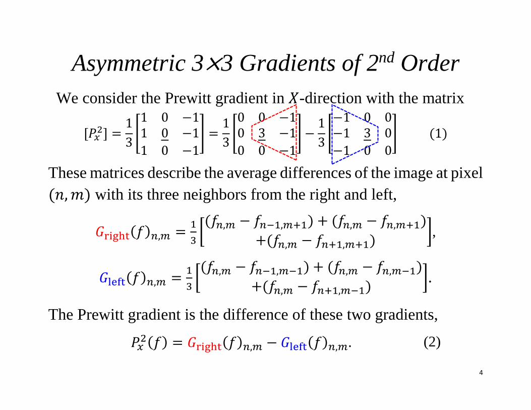
Asymmetric 3×3 Gradients of 2nd Order

We consider the Prewitt gradient in 𝑋-direction with the matrix

[𝑃𝑥2] =

1

3[1 0 −11 0 −1

1 0 −1

] =1

3[0 0 −10 3 −1

0 0 −1

] −1

3[−1 0 0−1 3 0

−1 0 0

] (1)

These matrices describe the average differences of the image at pixel

(𝑛,𝑚) with its three neighbors from the right and left,

𝐺right(𝑓)𝑛,𝑚 =1

3[(𝑓𝑛,𝑚 − 𝑓𝑛−1,𝑚+1) + (𝑓𝑛,𝑚 − 𝑓𝑛,𝑚+1)

+(𝑓𝑛,𝑚 − 𝑓𝑛+1,𝑚+1)],

𝐺left(𝑓)𝑛,𝑚 =1

3[(𝑓𝑛,𝑚 − 𝑓𝑛−1,𝑚−1) + (𝑓𝑛,𝑚 − 𝑓𝑛,𝑚−1)

+(𝑓𝑛,𝑚 − 𝑓𝑛+1,𝑚−1)].

The Prewitt gradient is the difference of these two gradients,

𝑃𝑥2(𝑓) = 𝐺right(𝑓)𝑛,𝑚 − 𝐺left(𝑓)𝑛,𝑚. (2)

5

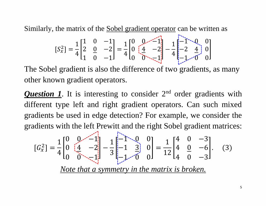
Similarly, the matrix of the Sobel gradient operator can be written as

[𝑆𝑥2] =

1

4[1 0 −12 0 −2

1 0 −1

] =1

4[0 0 −10 4 −2

0 0 −1

] −1

4[−1 0 0−2 4 0

−1 0 0

]

The Sobel gradient is also the difference of two gradients, as many

other known gradient operators.

Question 1. It is interesting to consider 2nd order gradients with

different type left and right gradient operators. Can such mixed

gradients be used in edge detection? For example, we consider the

gradients with the left Prewitt and the right Sobel gradient matrices:

[𝐺𝑥2] =

1

4[0 0 −10 4 −2

0 0 −1

] −1

3[−1 0 0−1 3 0

−1 0 0

] =1

12[4 0 −34 0 −6

4 0 −3

]. (3)

Note that a symmetry in the matrix is broken.

6

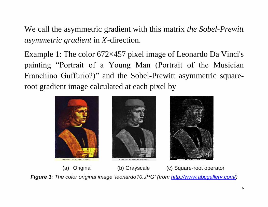
We call the asymmetric gradient with this matrix the Sobel-Prewitt

asymmetric gradient in 𝑋-direction.

Example 1: The color 672×457 pixel image of Leonardo Da Vinci's

painting “Portrait of a Young Man (Portrait of the Musician

Franchino Guffurio?)” and the Sobel-Prewitt asymmetric square-

root gradient image calculated at each pixel by

(a) Original (b) Grayscale (c) Square-root operator

Figure 1: The color original image ‘leonardo10.JPG’ (from http://www.abcgallery.com/)

7

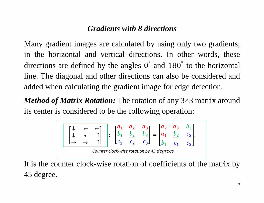
Gradients with 8 directions

Many gradient images are calculated by using only two gradients;

in the horizontal and vertical directions. In other words, these

directions are defined by the angles 0° and 180° to the horizontal

line. The diagonal and other directions can also be considered and

added when calculating the gradient image for edge detection.

Method of Matrix Rotation: The rotation of any 3×3 matrix around

its center is considered to be the following operation:

It is the counter clock-wise rotation of coefficients of the matrix by

45 degree.

Counter clock-wise rotation by 45 degrees

[

𝑎1 𝑎2 𝑎3𝑏1 𝑏2 𝑏3𝑐1 𝑐2 𝑐3

] =

𝑎2 𝑎3 𝑏3𝑎1 𝑏2 𝑐3

𝑏1 𝑐1 𝑐2

. :

[↓ ← ←↓ • ↑→ → ↑

]

8

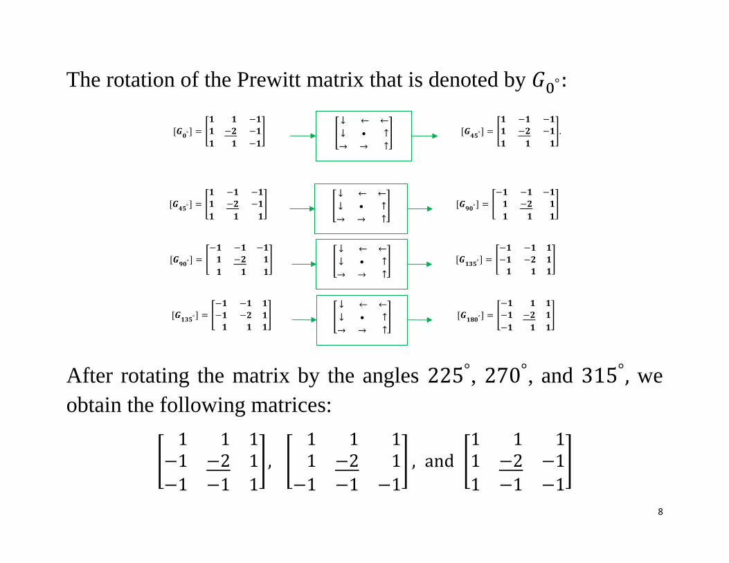
The rotation of the Prewitt matrix that is denoted by 𝐺0°:

After rotating the matrix by the angles 225°, 270°, and 315°, we

obtain the following matrices:

[1 1 1

−1 −2 1

−1 −1 1

], [1 1 11 −2 1

−1 −1 −1

] , and [1 1 11 −2 −1

1 −1 −1

]

[𝑮𝟎°] = [

𝟏 𝟏 −𝟏

𝟏 −𝟐 −𝟏

𝟏 𝟏 −𝟏

]

[↓ ← ←

↓ • ↑

→ → ↑

] [𝑮𝟒𝟓°] = [

𝟏 −𝟏 −𝟏

𝟏 −𝟐 −𝟏

𝟏 𝟏 𝟏

].

[𝑮𝟗𝟎°] = [

−𝟏 −𝟏 −𝟏

𝟏 −𝟐 𝟏

𝟏 𝟏 𝟏

]

[𝑮𝟏𝟑𝟓°

] = [−𝟏 −𝟏 𝟏

−𝟏 −𝟐 𝟏

𝟏 𝟏 𝟏

]

[↓ ← ←

↓ • ↑

→ → ↑

]

[𝑮𝟏𝟑𝟓°

] = [−𝟏 −𝟏 𝟏

−𝟏 −𝟐 𝟏

𝟏 𝟏 𝟏

]

[𝑮𝟏𝟖𝟎°

] = [−𝟏 𝟏 𝟏

−𝟏 −𝟐 𝟏

−𝟏 𝟏 𝟏

]

[↓ ← ←

↓ • ↑

→ → ↑

]

[𝑮𝟒𝟓°] = [

𝟏 −𝟏 −𝟏

𝟏 −𝟐 −𝟏

𝟏 𝟏 𝟏

]

[↓ ← ←

↓ • ↑

→ → ↑

] [𝑮𝟗𝟎°] = [

−𝟏 −𝟏 −𝟏

𝟏 −𝟐 𝟏

𝟏 𝟏 𝟏

]

9

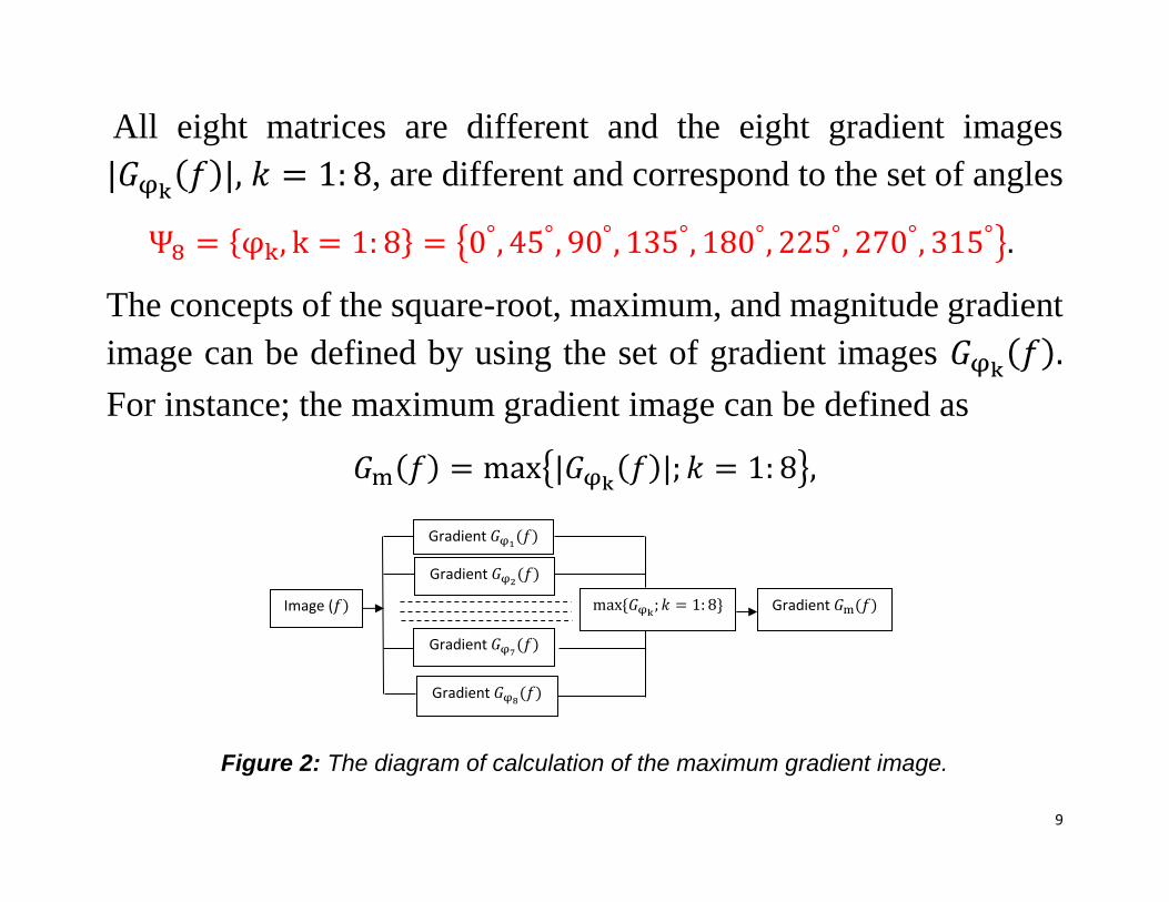
All eight matrices are different and the eight gradient images

|𝐺φk(𝑓)|, 𝑘 = 1: 8, are different and correspond to the set of angles

Ψ8 = {φk, k = 1: 8} = {0°, 45°, 90°, 135°, 180°, 225°, 270°, 315°}.

The concepts of the square-root, maximum, and magnitude gradient

image can be defined by using the set of gradient images 𝐺φk(𝑓).

For instance; the maximum gradient image can be defined as

𝐺m(𝑓) = max{|𝐺φk(𝑓)|; 𝑘 = 1: 8},

Figure 2: The diagram of calculation of the maximum gradient image.

Image (𝑓)

Gradient 𝐺φ1(𝑓)

Gradient 𝐺φ8(𝑓)

Gradient 𝐺m(𝑓) max{𝐺φk; 𝑘 = 1: 8}

Gradient 𝐺φ7(𝑓)

Gradient 𝐺φ2(𝑓)

10

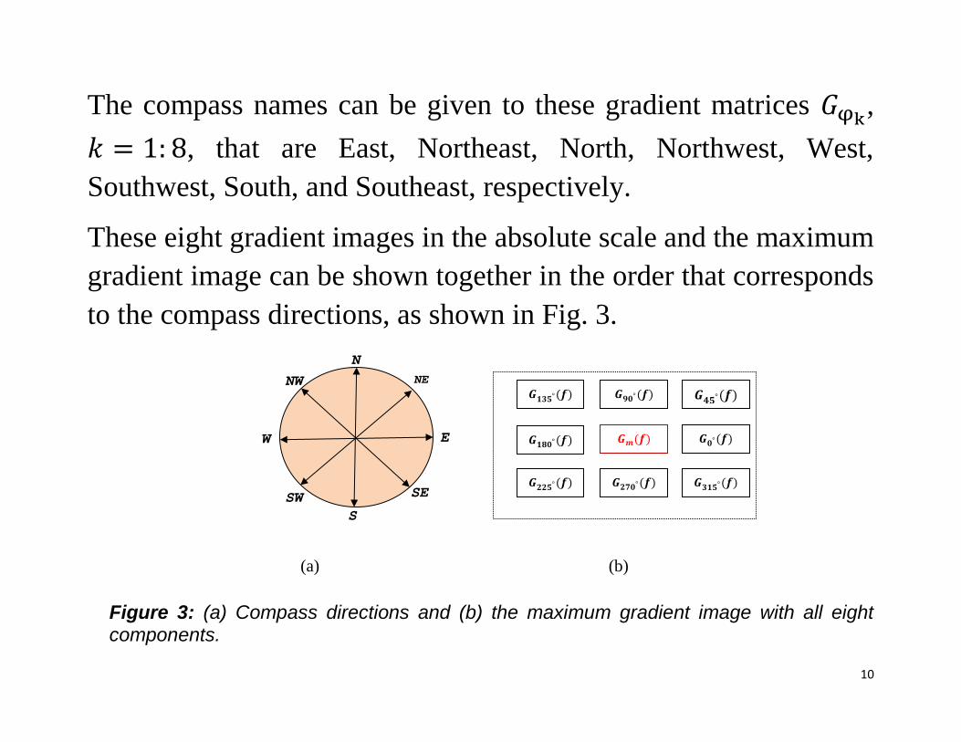
The compass names can be given to these gradient matrices 𝐺φk,

𝑘 = 1: 8, that are East, Northeast, North, Northwest, West,

Southwest, South, and Southeast, respectively.

These eight gradient images in the absolute scale and the maximum

gradient image can be shown together in the order that corresponds

to the compass directions, as shown in Fig. 3.

(a) (b)

Figure 3: (a) Compass directions and (b) the maximum gradient image with all eight components.

N

E W

S

NE NW

SW SE

𝑮𝒎(𝒇) 𝑮𝟎°(𝒇) 𝑮𝟏𝟖𝟎°(𝒇)

𝑮𝟐𝟕𝟎°(𝒇) 𝑮𝟐𝟐𝟓°(𝒇) 𝑮𝟑𝟏𝟓°(𝒇)

𝑮𝟏𝟑𝟓°(𝒇) 𝑮𝟗𝟎°(𝒇) 𝑮𝟒𝟓°(𝒇)

11

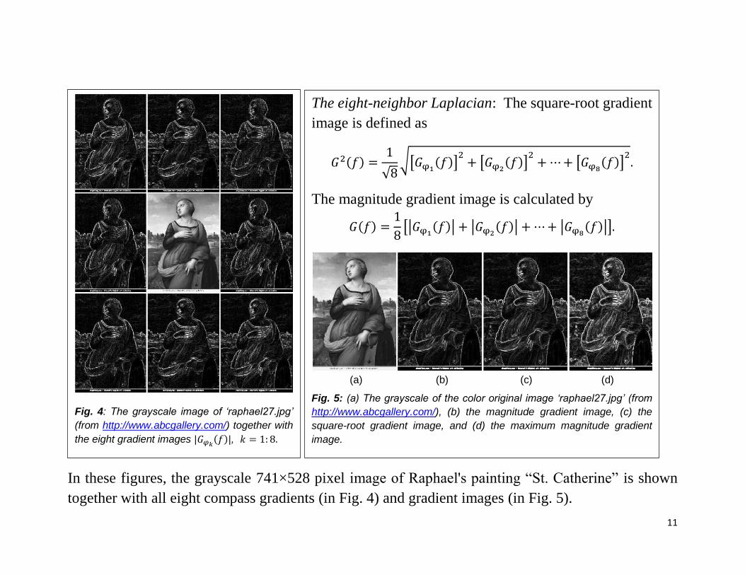
In these figures, the grayscale 741×528 pixel image of Raphael's painting “St. Catherine” is shown

together with all eight compass gradients (in Fig. 4) and gradient images (in Fig. 5).

Fig. 4: The grayscale image of ‘raphael27.jpg’

(from http://www.abcgallery.com/) together with

the eight gradient images |𝐺𝜑𝑘(𝑓)|, 𝑘 = 1: 8.

The eight-neighbor Laplacian: The square-root gradient

image is defined as

𝐺2(𝑓) =1

√8√[𝐺φ1(𝑓)]

2+ [𝐺φ2(𝑓)]

2+⋯+ [𝐺φ8(𝑓)]

2.

The magnitude gradient image is calculated by

𝐺(𝑓) =1

8[|𝐺φ1(𝑓)| + |𝐺φ2(𝑓)| + ⋯+ |𝐺φ8(𝑓)|].

(a) (b) (c) (d)

Fig. 5: (a) The grayscale of the color original image ‘raphael27.jpg’ (from

http://www.abcgallery.com/), (b) the magnitude gradient image, (c) the

square-root gradient image, and (d) the maximum magnitude gradient

image.

12

All eight gradient images are different, since the matrices of

rotations are different, and they are shown in Table 1.

[𝐺0°]

=1

5[1 1 −11 −2 −1

1 1 −1

]

[𝐺45°]

=1

5[1 −1 −11 −2 −1

1 1 1

]

[𝐺90°]

=1

5[−1 −1 −11 −2 1

1 1 1

]

[𝐺135°]

=1

5[−1 −1 1−1 −2 11 1 1

]

[𝐺180°]

=1

5[−1 1 1−1 −2 1

−1 1 1

]

[𝐺225°]

=1

5[1 1 1

−1 −2 1

−1 −1 1

]

[𝐺270°]

=1

5[1 1 11 −2 1

−1 −1 −1

]

[𝐺315°]

=1

5[1 1 11 −2 −1

1 −1 −1

]

∑[𝐺φk]

=16

5∙1

8[1 1 11 −8 1

1 1 1

]

Table 1: Matrices of gradient operators.

13

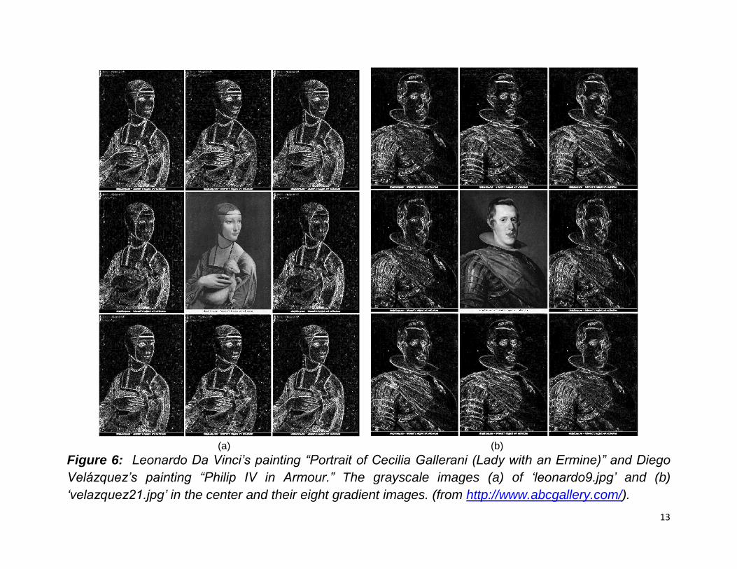
(a) (b)

Figure 6: Leonardo Da Vinci’s painting “Portrait of Cecilia Gallerani (Lady with an Ermine)” and Diego

Velázquez’s painting “Philip IV in Armour.” The grayscale images (a) of ‘leonardo9.jpg’ and (b)

‘velazquez21.jpg’ in the center and their eight gradient images. (from http://www.abcgallery.com/).

14

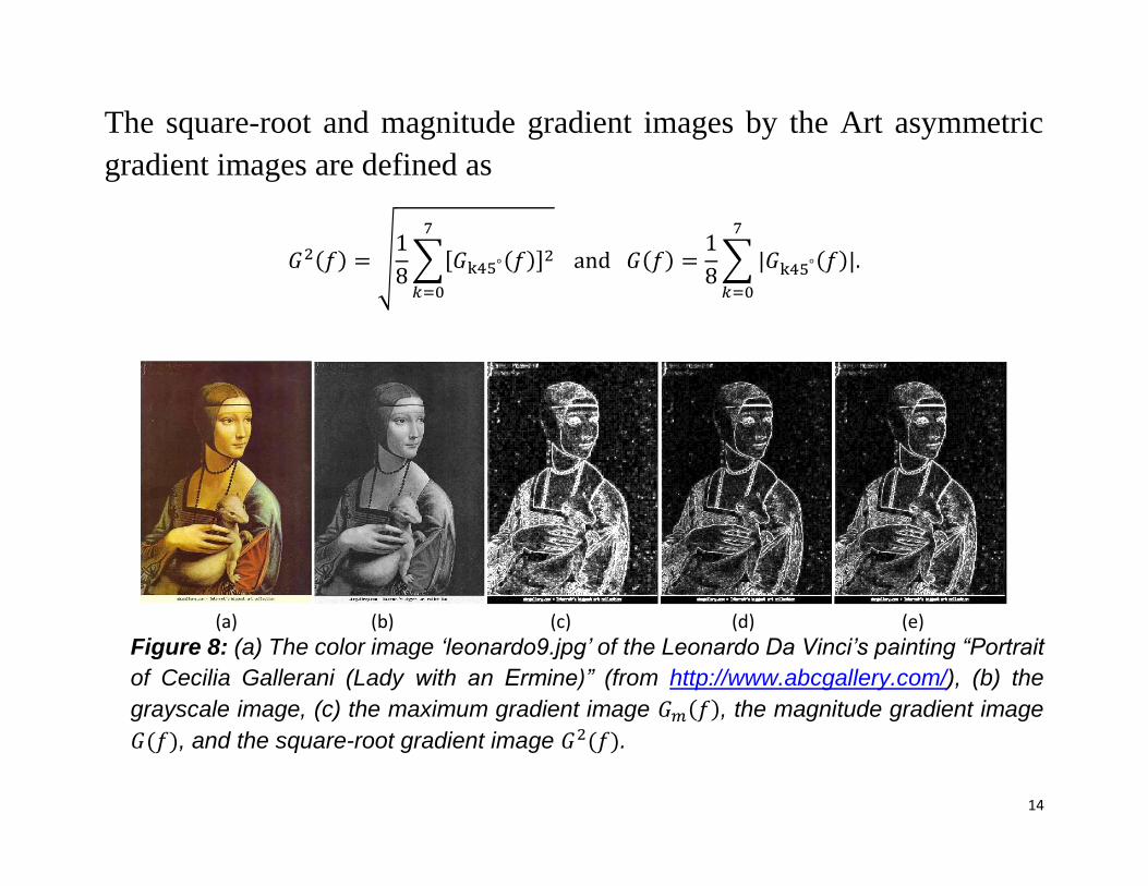
The square-root and magnitude gradient images by the Art asymmetric

gradient images are defined as

𝐺2(𝑓) = √1

8∑[𝐺k45°(𝑓)]

2

7

𝑘=0

and 𝐺(𝑓) =1

8∑ |𝐺k45°(𝑓)|

7

𝑘=0

.

(a) (b) (c) (d) (e)

Figure 8: (a) The color image ‘leonardo9.jpg’ of the Leonardo Da Vinci’s painting “Portrait

of Cecilia Gallerani (Lady with an Ermine)” (from http://www.abcgallery.com/), (b) the

grayscale image, (c) the maximum gradient image 𝐺𝑚(𝑓), the magnitude gradient image

𝐺(𝑓), and the square-root gradient image 𝐺2(𝑓).

15

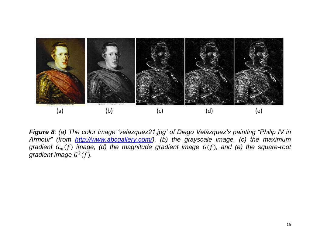
(a) (b) (c) (d) (e)

Figure 8: (a) The color image ‘velazquez21.jpg’ of Diego Velázquez’s painting “Philip IV in Armour” (from http://www.abcgallery.com/), (b) the grayscale image, (c) the maximum gradient 𝐺𝑚(𝑓) image, (d) the magnitude gradient image 𝐺(𝑓), and (e) the square-root

gradient image 𝐺2(𝑓).

16

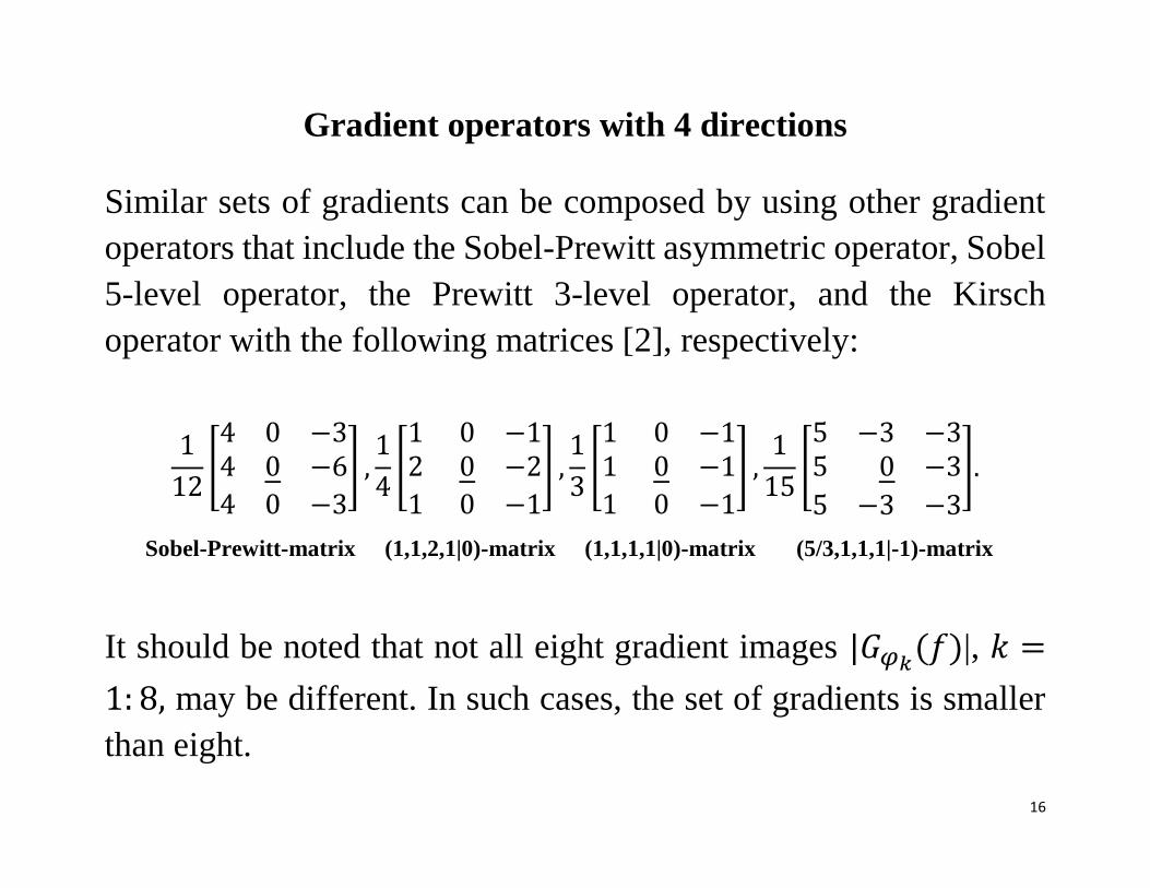
Gradient operators with 4 directions

Similar sets of gradients can be composed by using other gradient

operators that include the Sobel-Prewitt asymmetric operator, Sobel

5-level operator, the Prewitt 3-level operator, and the Kirsch

operator with the following matrices [2], respectively:

1

12[4 0 −34 0 −6

4 0 −3

] ,1

4[1 0 −12 0 −2

1 0 −1

] ,1

3[1 0 −11 0 −1

1 0 −1

] ,1

15[5 −3 −35 0 −3

5 −3 −3

].

Sobel-Prewitt-matrix (1,1,2,1|0)-matrix (1,1,1,1|0)-matrix (5/3,1,1,1|-1)-matrix

It should be noted that not all eight gradient images |𝐺𝜑𝑘(𝑓)|, 𝑘 =

1: 8, may be different. In such cases, the set of gradients is smaller

than eight.

17

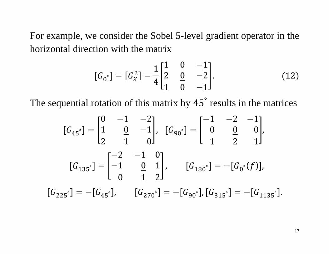
For example, we consider the Sobel 5-level gradient operator in the

horizontal direction with the matrix

[𝐺0°] = [𝐺𝑥2] =

1

4[1 0 −12 0 −2

1 0 −1

]. (12)

The sequential rotation of this matrix by 45° results in the matrices

[𝐺45°] = [0 −1 −21 0 −1

2 1 0

], [𝐺90°] = [−1 −2 −10 0 0

1 2 1

],

[𝐺135°] = [−2 −1 0−1 0 1

0 1 2

] , [𝐺180°] = −[𝐺0°(𝑓)],

[𝐺225°] = −[𝐺45°], [𝐺270°] = −[𝐺90°], [𝐺315°] = −[𝐺1135°].

18

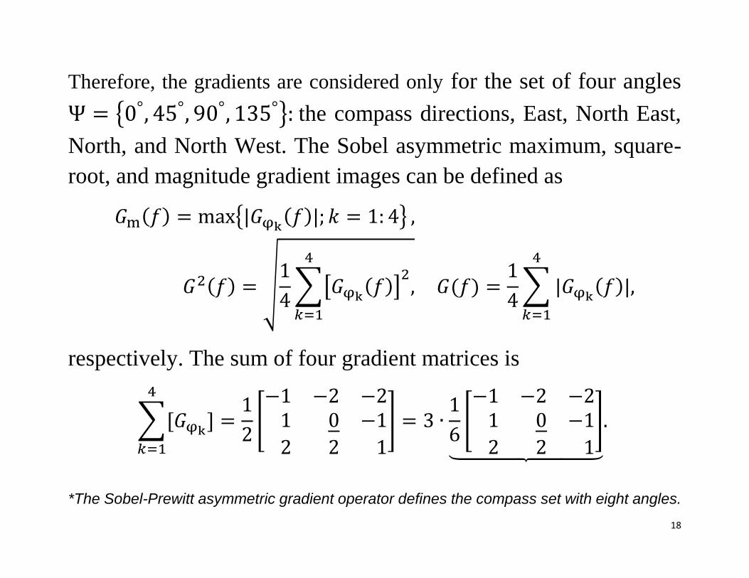
Therefore, the gradients are considered only for the set of four angles

Ψ = {0°, 45°, 90°, 135°}: the compass directions, East, North East,

North, and North West. The Sobel asymmetric maximum, square-

root, and magnitude gradient images can be defined as

𝐺m(𝑓) = max{|𝐺φk(𝑓)|; 𝑘 = 1: 4} ,

𝐺2(𝑓) = √1

4∑[𝐺φk(𝑓)]

2,

4

𝑘=1

𝐺(𝑓) =1

4∑ |𝐺φk(𝑓)|,

4

𝑘=1

respectively. The sum of four gradient matrices is

∑[𝐺φk]

4

𝑘=1

=1

2[−1 −2 −21 0 −1

2 2 1

] = 3 ∙1

6[−1 −2 −21 0 −1

2 2 1

]⏟

.

*The Sobel-Prewitt asymmetric gradient operator defines the compass set with eight angles.

19

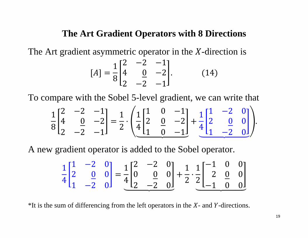
The Art Gradient Operators with 8 Directions

The Art gradient asymmetric operator in the 𝑋-direction is

[𝐴] =1

8[2 −2 −14 0 −2

2 −2 −1

]. (14)

To compare with the Sobel 5-level gradient, we can write that

1

8[2 −2 −14 0 −2

2 −2 −1

] =1

2· (1

4[1 0 −12 0 −2

1 0 −1

]⏟

+1

4[1 −2 02 0 0

1 −2 0

]⏟

).

A new gradient operator is added to the Sobel operator.

1

4[1 −2 02 0 0

1 −2 0

] =1

4[2 −2 00 0 0

2 −2 0

]⏟

+1

2·1

2[−1 0 02 0 0

−1 0 0

]⏟

*It is the sum of differencing from the left operators in the 𝑋- and 𝑌-directions.

20

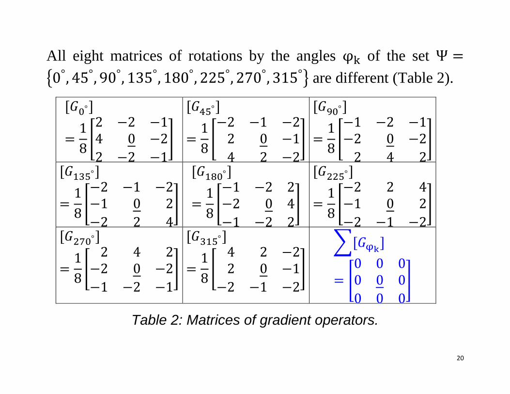
All eight matrices of rotations by the angles φk of the set Ψ =

{0°, 45°, 90°, 135°, 180°, 225°, 270°, 315°} are different (Table 2).

[𝐺0°]

=1

8[2 −2 −14 0 −2

2 −2 −1

]

[𝐺45°]

=1

8[−2 −1 −22 0 −1

4 2 −2

]

[𝐺90°]

=1

8[−1 −2 −1−2 0 −2

2 4 2

]

[𝐺135°]

=1

8[−2 −1 −2−1 0 2

−2 2 4

]

[𝐺180°]

=1

8[−1 −2 2−2 0 4

−1 −2 2

]

[𝐺225°]

=1

8[−2 2 4−1 0 2

−2 −1 −2

]

[𝐺270°]

=1

8[2 4 2

−2 0 −2

−1 −2 −1

]

[𝐺315°]

=1

8[4 2 −22 0 −1

−2 −1 −2

]

∑[𝐺φk]

= [0 0 00 0 0

0 0 0

]

Table 2: Matrices of gradient operators.

21

Portrait Image Representation for Recognition

We consider the grayscale facial image representation, or

description, which is based on the local binary patterns (LBP) over

the whole facial image [1,2]. We describe this representation in

terms of simple gradient operators with following composition of

the 8-bit LBP image and its histogram, which can be used as the

feature in classification of facial images.

The main parts of representation of the grayscale 𝑁 ×𝑀–pixel

facial image 𝑓𝑛,𝑚 are shown in the block-diagram of Fig. 9.

Figure 9. The block-diagram of the facial image representation.

8 Rotation Gradient-Based Local Binary Patterns (8R-GLBP)

Grayscale

Image

8R-Gradient

image

Gaussian

filter

LBP/ULBP

image

Histogram of

LBP/ULBP

22

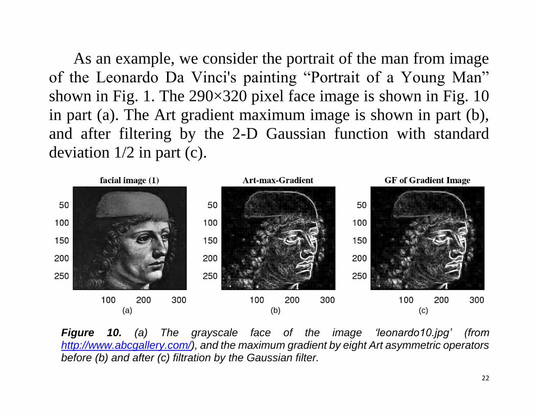
As an example, we consider the portrait of the man from image

of the Leonardo Da Vinci's painting “Portrait of a Young Man”

shown in Fig. 1. The 290×320 pixel face image is shown in Fig. 10

in part (a). The Art gradient maximum image is shown in part (b),

and after filtering by the 2-D Gaussian function with standard

deviation 1/2 in part (c).

(a) (b) (c)

Figure 10. (a) The grayscale face of the image ‘leonardo10.jpg’ (from http://www.abcgallery.com/), and the maximum gradient by eight Art asymmetric operators before (b) and after (c) filtration by the Gaussian filter.

23

Figure 11 shows the LBP image of this face in part (a) and its histogram

with the range [0,255] in part (b).

Figure 11. (a) The local binary pattern image and (b) and the histogram of the image.

The concept of the uniform LBP was introduced to reduce the range of the

histogram from [0,255] to [0,58]. The window for calculating the local

pattern is 3×3 and the ULBP is calculated recursively in 8 stages, by using

the special mapping to the patterns in number 59.

24

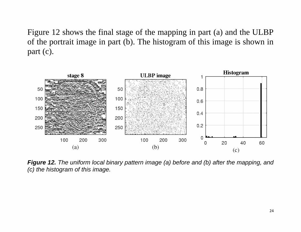
Figure 12 shows the final stage of the mapping in part (a) and the ULBP

of the portrait image in part (b). The histogram of this image is shown in

part (c).

Figure 12. The uniform local binary pattern image (a) before and (b) after the mapping, and (c) the histogram of this image.

25

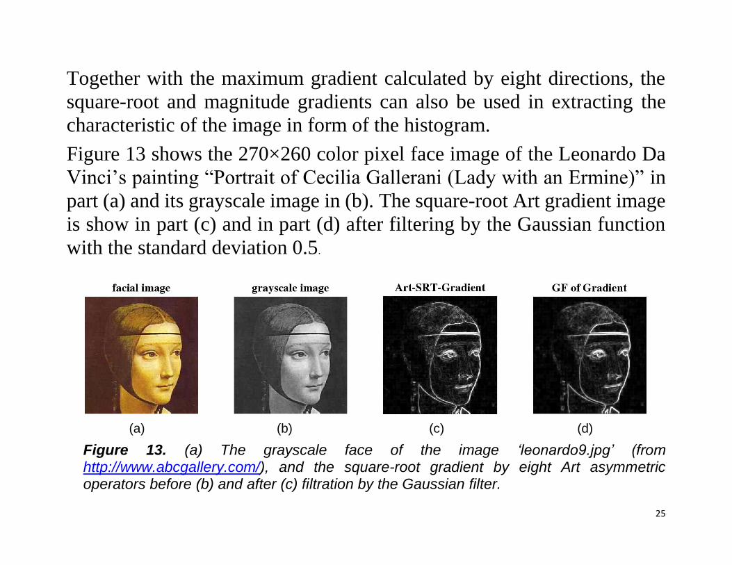
Together with the maximum gradient calculated by eight directions, the

square-root and magnitude gradients can also be used in extracting the

characteristic of the image in form of the histogram.

Figure 13 shows the 270×260 color pixel face image of the Leonardo Da

Vinci’s painting “Portrait of Cecilia Gallerani (Lady with an Ermine)” in

part (a) and its grayscale image in (b). The square-root Art gradient image

is show in part (c) and in part (d) after filtering by the Gaussian function

with the standard deviation 0.5.

(a) (b) (c) (d)

Figure 13. (a) The grayscale face of the image ‘leonardo9.jpg’ (from http://www.abcgallery.com/), and the square-root gradient by eight Art asymmetric operators before (b) and after (c) filtration by the Gaussian filter.

26

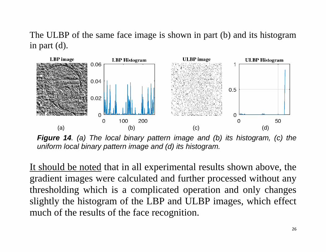
The ULBP of the same face image is shown in part (b) and its histogram

in part (d).

(a) (b) (c) (d)

Figure 14. (a) The local binary pattern image and (b) its histogram, (c) the uniform local binary pattern image and (d) its histogram.

It should be noted that in all experimental results shown above, the

gradient images were calculated and further processed without any

thresholding which is a complicated operation and only changes

slightly the histogram of the LBP and ULBP images, which effect

much of the results of the face recognition.

27

Summary

A novel face recognition approach is proposed, by using multiple

feature fusion across color, spatial and frequency domains. The

proposed approach is useful and applicable not only for face

recognition, but also for object recognition.

We are planning to evaluate the presented face recognition concept,

by using the color FERET database: http://www.face-

rec.org/databases/.

References 1. A.M. Grigoryan, S.S. Agaian, Practical Quaternion and Octonion Imaging With

MATLAB, SPIE PRESS, 2018. 2. A.M. Grigoryan, S.S. Agaian, “Color facial image representation with new quaternion

gradients,” Image Processing: Algorithms and Systems, IS&T Electronic Imaging Symposium, p. 6, Burlingame, CA, 28 Jan.-2 Feb 2018.

3. A.M. Grigoryan, S.S. Agaian, “Two general models for gradient operators in imaging,” Proceedings of IS&T International Symposium, Electronic Imaging: Algorithms and Systems, 28 Jan.-2 Feb., Burlingame, CA, 2018. ...