a_study on mobile production
TRANSCRIPT

8/8/2019 A_study on Mobile Production
http://slidepdf.com/reader/full/astudy-on-mobile-production 1/66
A STUDY ON MOBILE PRODUCTION
BY
RAMU THIAGARAJAN
OF
GREAT EASTERN MANAGEMENT SCHOOL, CHENNAI.
2010-2011
A PROJECT REPORT
SUBMITTED TO THE DEPARTMENT OF MANAGEMENT STUDIES
IN PARTIAL FULFILLMENT OF THE REQUIREMENTS
FOR THE AWARD OF DEGREE
OF
MASTER OF BUSINESS ADMINISTRATION
8/8/2019 A_study on Mobile Production
http://slidepdf.com/reader/full/astudy-on-mobile-production 2/66
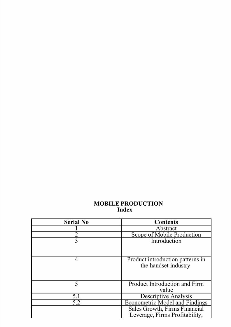
MOBILE PRODUCTIONIndex
Serial No Contents
1 Abstract2 Scope of Mobile Production3 Introduction
4 Product introduction patterns inthe handset industry
5 Product Introduction and Firmvalue5 1 Descriptive Analysis

8/8/2019 A_study on Mobile Production
http://slidepdf.com/reader/full/astudy-on-mobile-production 3/66
Estimation Results of RandomEffects Model
Description of the Data
6 Conceptual Framework andRelated Literature
7 Institutional Context8 Hypothesis Data and Empherical
Design9 Empherical Specification and
Strategy10 Results and Analysis11 Cross Sectional Results
12 Conclusion13 Bibliography14 Descriptive Statistics
14(i) Unbalanced Panel14(ii) Balanced Panel14(iii) Balanced Panel Correlations14(iv) Adoption of Mobile IT Networks
and the Boundary of the Firm14(v) Adoption of Mobile IT Networks
and the Productivity14(vi) Complementarities
15 Total Factor Productivity inQuantities (TFPQ)
ABSTRACT: We study the effect of new product introduction on firm value. Using a uniquesample on mobile phone handset introduction by 16 major handset manufacturers over 10years, we distinguish between imitative product introduction and truly innovative productintroduction. We find that while most product introduction is imitative, both types of innovation increase firm value. However, truly innovative innovation is found to increase firmvalue by more than imitative introductions.
Keywords: Product innovation, mobile telephony, firm value.
1. Introduction
The markets for wireless technologies are the origin of new products that can be applied
throughout the economy and of which widespread adoption provides substantial growth
8/8/2019 A_study on Mobile Production
http://slidepdf.com/reader/full/astudy-on-mobile-production 4/66
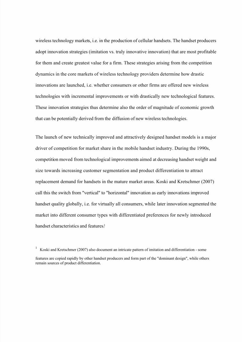
wireless technology markets, i.e. in the production of cellular handsets. The handset producers
adopt innovation strategies (imitation vs. truly innovative innovation) that are most profitable
for them and create greatest value for a firm. These strategies arising from the competition
dynamics in the core markets of wireless technology providers determine how drastic
innovations are launched, i.e. whether consumers or other firms are offered new wireless
technologies with incremental improvements or with drastically new technological features.
These innovation strategies thus determine also the order of magnitude of economic growth
that can be potentially derived from the diffusion of new wireless technologies.
The launch of new technically improved and attractively designed handset models is a major
driver of competition for market share in the mobile handset industry. During the 1990s,
competition moved from technological improvements aimed at decreasing handset weight and
size towards increasing customer segmentation and product differentiation to attract
replacement demand for handsets in the mature market areas. Koski and Kretschmer (2007)
call this the switch from "vertical" to "horizontal" innovation as early innovations improved
handset quality globally, i.e. for virtually all consumers, while later innovation segmented the
market into different consumer types with differentiated preferences for newly introduced
handset characteristics and features.1
1Koski and Kretschmer (2007) also document an intricate pattern of imitation and differentiation - some
features are copied rapidly by other handset producers and form part of the "dominant design", while othersremain sources of product differentiation.
8/8/2019 A_study on Mobile Production
http://slidepdf.com/reader/full/astudy-on-mobile-production 5/66
2
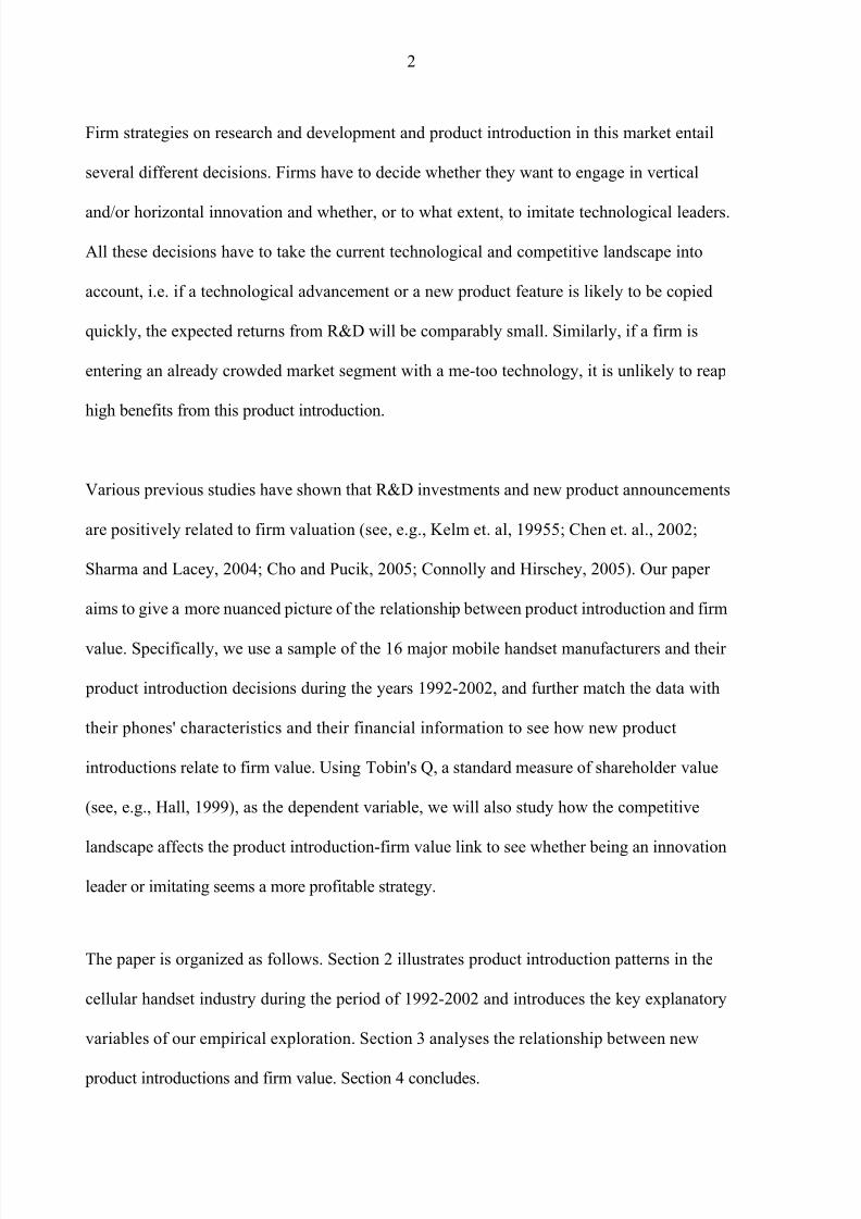
Firm strategies on research and development and product introduction in this market entail
several different decisions. Firms have to decide whether they want to engage in vertical
and/or horizontal innovation and whether, or to what extent, to imitate technological leaders.
All these decisions have to take the current technological and competitive landscape into
account, i.e. if a technological advancement or a new product feature is likely to be copied
quickly, the expected returns from R&D will be comparably small. Similarly, if a firm is
entering an already crowded market segment with a me-too technology, it is unlikely to reap
high benefits from this product introduction.
Various previous studies have shown that R&D investments and new product announcements
are positively related to firm valuation (see, e.g., Kelm et. al, 19955; Chen et. al., 2002;
Sharma and Lacey, 2004; Cho and Pucik, 2005; Connolly and Hirschey, 2005). Our paper
aims to give a more nuanced picture of the relationship between product introduction and firm
value. Specifically, we use a sample of the 16 major mobile handset manufacturers and their
product introduction decisions during the years 1992-2002, and further match the data with
their phones' characteristics and their financial information to see how new product
introductions relate to firm value. Using Tobin's Q, a standard measure of shareholder value
(see, e.g., Hall, 1999), as the dependent variable, we will also study how the competitive
landscape affects the product introduction-firm value link to see whether being an innovation
leader or imitating seems a more profitable strategy.
The paper is organized as follows. Section 2 illustrates product introduction patterns in the
cellular handset industry during the period of 1992-2002 and introduces the key explanatory
variables of our empirical exploration. Section 3 analyses the relationship between new
product introductions and firm value. Section 4 concludes.
8/8/2019 A_study on Mobile Production
http://slidepdf.com/reader/full/astudy-on-mobile-production 6/66
3
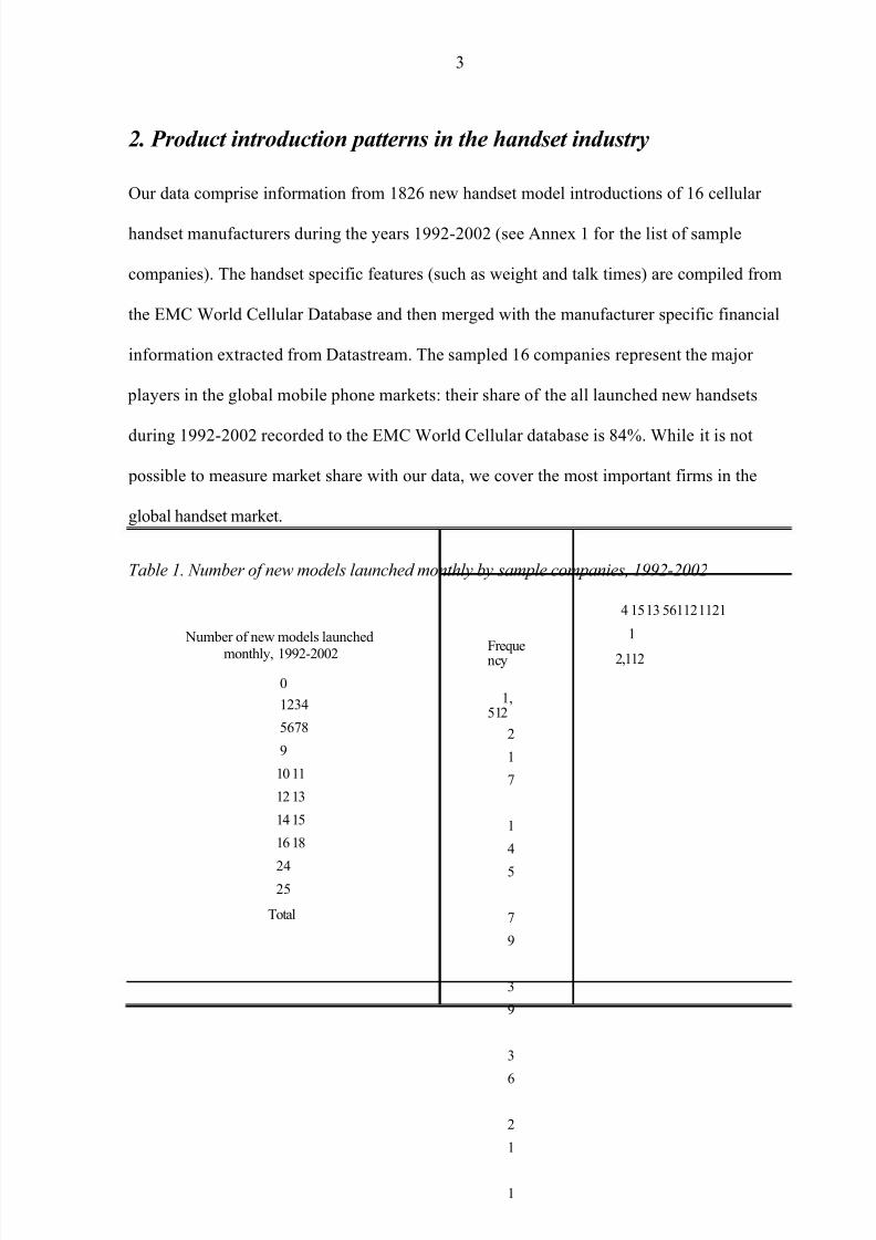
2. Product introduction patterns in the handset industry
Our data comprise information from 1826 new handset model introductions of 16 cellular
handset manufacturers during the years 1992-2002 (see Annex 1 for the list of sample
companies). The handset specific features (such as weight and talk times) are compiled from
the EMC World Cellular Database and then merged with the manufacturer specific financial
information extracted from Datastream. The sampled 16 companies represent the major
players in the global mobile phone markets: their share of the all launched new handsets
during 1992-2002 recorded to the EMC World Cellular database is 84%. While it is not
possible to measure market share with our data, we cover the most important firms in the
global handset market.
Table 1. Number of new models launched monthly by sample companies, 1992-2002
Number of new models launched
monthly, 1992-2002
0
1234
5678
9
10 11
12 13
14 15
16 18
2425
Total
Frequency
1,512
2
1
7
1
4
5
7
9
3
9
3
6
2
4 15 13 561121121
1
2,112

8/8/2019 A_study on Mobile Production
http://slidepdf.com/reader/full/astudy-on-mobile-production 7/66
% of new handsets launched bysample firms
71.59%
10.27% 6.87%
3.74% 1.85% 1.70%
0.99% 0.66% 0.71%
0.62% 0.24% 0.28%
0.05
%
0.05
%
0.09
%
0.05
%
0.05%
0.09%
0.05%
0.05%
100.00%
8/8/2019 A_study on Mobile Production
http://slidepdf.com/reader/full/astudy-on-mobile-production 8/66
4
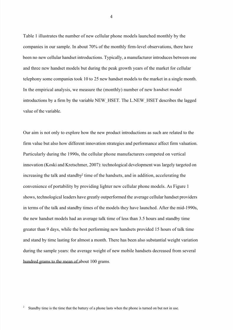
Table 1 illustrates the number of new cellular phone models launched monthly by the
companies in our sample. In about 70% of the monthly firm-level observations, there have
been no new cellular handset introductions. Typically, a manufacturer introduces between one
and three new handset models but during the peak growth years of the market for cellular
telephony some companies took 10 to 25 new handset models to the market in a single month.
In the empirical analysis, we measure the (monthly) number of new handset model
introductions by a firm by the variable NEW_HSET. The L.NEW_HSET describes the lagged
value of the variable.
Our aim is not only to explore how the new product introductions as such are related to the
firm value but also how different innovation strategies and performance affect firm valuation.
Particularly during the 1990s, the cellular phone manufacturers competed on vertical
innovation (Koski and Kretschmer, 2007): technological development was largely targeted on
increasing the talk and standby2 time of the handsets, and in addition, accelerating the
convenience of portability by providing lighter new cellular phone models. As Figure 1
shows, technological leaders have greatly outperformed the average cellular handset providers
in terms of the talk and standby times of the models they have launched. After the mid-1990s,
the new handset models had an average talk time of less than 3.5 hours and standby time
greater than 9 days, while the best performing new handsets provided 15 hours of talk time
and stand by time lasting for almost a month. There has been also substantial weight variation
during the sample years: the average weight of new mobile handsets decreased from several
hundred grams to the mean of about 100 grams.

8/8/2019 A_study on Mobile Production
http://slidepdf.com/reader/full/astudy-on-mobile-production 9/66
5
Figure 1. Technological leaders vs. average firms: talk and standby times
Technological leader vs. average firms: talk and standby times
1000
900
800
700
600
500
400
300
200
100
0
Av.talk time (minutes)
Av.standby time (hours)
Max talk time
Max standby time
1992 1993 1994 1995 1996 1997 1998 1999 2000 2001 2002
We use the variable TECH_LEAD to capture the (relative) vertical innovation performance of
the firm. The variable is calculated by adding up three dummy variables that take value 1 if
the handset models a firm introduced during the sample year: i) have greater talk time, ii)
have greater standby time and iii) are lighter, on average, than the handset models introduced
in the same year, and 0 otherwise. This constructed variable thus takes values between 0 and 3
- 0 indicates that a firm is a complete imitator in vertical innovation (i.e. the average new
handset models on the market outperform the focal firm's new handsets in all three
dimensions), and 3 indicates that the firm belongs to the vertical innovation leaders (i.e. its
new handsets have been superior to the average models in regard to their standby and talk
times and weight).
Successful (horizontal) product differentiation may soften competition and thus generate

8/8/2019 A_study on Mobile Production
http://slidepdf.com/reader/full/astudy-on-mobile-production 10/66
6
sufficient data concerning the sample firms' horizontal innovation patterns such as the
availability of the games and design features (e.g. clamshells) for the empirical estimations.
However, as the inclusion of the additional features to the given handset model decreases its
talk and standby time, we can use the dispersion in the talk and standby times of the firm's
new handset models at a given time as indicator of its horizontal innovation strategy. The
intuition here is that if that if all new handset models of the firm at a given time were
homogeneous in terms of the additional features, the firm would produce new handsets with
equal (maximum possible for a firm) talk and standby times. Thus, higher variation in talk
and standby times also implies more differentiated products. Therefore, we use the variables
CV_TALK and CV_STANDBY to measure the coefficient of variation (i.e. mean divided by
standard deviation) in the talk and standby times, respectively, of the firm's new handset
models in a given year. Since there is a tradeoff between talk and standby times and the
handset size as well, we use the variable SIZE to control for the average size (i.e. log of
handset height*weight*length) of the handsets the firm has launched that year.
Also, the firm's product mix and market strategy may influence its valuation. Competition
between different technological standards has characterized the markets for cellular telephony
throughout the sample time. The cellular telephone manufacturers have launched different
mixes of new phones for analogous and digital standards GSM, CDMA, TDMA and
PHSPDC network connections. These standard choices also reflect the manufacturers'
geographical market strategies as the regional differences in the standard choices for the
mobile telephony networks have been substantial (see, e.g., Koski, 2006). We control for the
firm's product mix strategy in terms of technological standards by the variable
CV_STANDARD. This variable is the number of new GSM, CMDA, TDMA, PHSPDC and
analogue handset models the firm has launched at a given year. The variable gets value 0 if

8/8/2019 A_study on Mobile Production
http://slidepdf.com/reader/full/astudy-on-mobile-production 11/66
7
the greater the mix of phones using different technological standards (i.e. value 5 means that
the firm has launched new cellular phone models compatible with all 4 digital standards and
with one or more analogue standards)
3. Product introductions and firm value
3.1 Descriptive analysis
We use the following approximation of the theoretical Tobin's Q measure to measure firm
value: (common shares outstanding * prices + book value total assets - common equity) /
book value total assets. Figure 2 compares the monthly averages of Tobin's Q values of firms
which introduced new cellular handset models to those of the firms that launched no new
handset models during the observed month. The average Tobin's Q over all observed months
Figure 2. Tobin's Q monthly averages: firms with new handset introductions vs. no new handsets
Tobin'q monthly average for firms with new handset introductions vs. no new handsets
4
3.5
3
2.5
New handset introduction(s)2
No new handset introductions
1.5
1
0.5
0
1992 1993 1994 1995 1996 1997 1998 1999 2000 2001 2002
8/8/2019 A_study on Mobile Production
http://slidepdf.com/reader/full/astudy-on-mobile-production 12/66
8
during the years 1992-2002 is about 2 for the manufacturers introducing new handset models,
whereas the corresponding number is about 1.4 for firms with no new mobile handsets. The t-
test further indicates that this difference is statistically significant, providing preliminary
evidence on the positive relationship between the cellular phone manufacturers' market value
and new handset model introductions.
Figure 2 also illustrates that the stock market value of the cellular handset manufacturers
rapidly increased at the end of the 1990s when the global market for the cellular handsets
witnessed a fast expansion as the demand for the cellular handsets were strongly growing. The
underlying reason for this growth pattern, however, relates rather to the "dot-com boom", the
general overvaluation of the IT stocks in the end of the 1990s. In 2001, when the share prices
of many IT companies crashed, we also observe a sharp decline in the share values of the
stocks of the major cellular handset manufacturers. As the sample cellular handset
manufacturers had a viable business models, unlike many newly established dot-com
companies, the stock market valuation of the handset manufacturers was not collapsing but
just returning to the level it was before the period of general overvaluation of the IT stocks.
3.2. Econometric model and findings
Our main interest is in the relationship between product launch (imitative and innovative) and
firm value. At the same time, there are a number of control variables we need to consider
because they are expected to have an impact on firm value in their own right. We chose to use
the random effects model as our interest is to use information from the 16 sampled companies
to draw inferences regarding all firms in the industry3. We use the following econometric
3 The disadvantage of the random effect model compared to the fixed effect model is that former one does not allow,

8/8/2019 A_study on Mobile Production
http://slidepdf.com/reader/full/astudy-on-mobile-production 13/66
9
model in our estimations aiming at explaining variation in the firm value of the mobile
handset manufacturers during the years 1992-2002:
Log (Tobin' sQit
) = α0+ α
1 NEW _ HSET
it + α
2L1. NEW _ HSET
it + α
3TECH _
LEADit
+ α4SIZE
it + α
5CV _ STANDBY
it + α
6CV _ TALK
it + α
7CV _
STANDARDit
+ α8SALES _ GROWTH
it + α
9DEBT
it + α
10PROFITABILITY
it
+
12.2002
∑α t dm + ∑α ydy + ∑α idi +
ui+ ε
it 2002 16
t = 1.1992 y= 1992 i= 1
The subscripts i and t denote, respectively, firm- and month-specific observations from
January 1992 to December 2002 among the samped 16 companies. The dummy variables dm,
dy and di control, respectively, for fixed month, year, and firm effects. In addition to t the
standard error term, ha εit , the model includes firm-specific, time-constant random
heterogeneity term, ui.
In addition to the major explanatory variables of interest describing the firms' innovation
performance and strategies, we use the following covariates:4
Sales growth may raise investors' expectations about a firm's future returns and thus affect its
market valuation. Growing firms are expected to perform well in the future in two ways: First,
higher sales simply enable them to reap higher profits. Second, fast-growing firms may gain
market share on their rivals, giving them a stronger position in the market. However, as most
of the products in our sample are multiproduct firms, we cannot account for this second

8/8/2019 A_study on Mobile Production
http://slidepdf.com/reader/full/astudy-on-mobile-production 14/66
4 We do not report the coefficients for year, month and firm dummies. Results on these are available on request.

8/8/2019 A_study on Mobile Production
http://slidepdf.com/reader/full/astudy-on-mobile-production 15/66
10
Firm's financial leverage is also expected to have an effect on firm value. On the one hand,
higher financial leverage may indicate a higher likelihood of financial distress and
bankruptcy. On the other hand, financial leverage may also indicate that an investor's share of
total equity stretches further. Although it is an empirical question which of the effects
dominates, we need to control for these effects. We do this by including the variable DEBT,
defined by (Total Assets - Total Equity) / Total Assets, in our regressions.
Firm profitability will also have an effect on firm value. However, in a market characterized
by high growth like the mobile handset industry, the link between current profits and overall
firm value may be tenuous.5 We define PROFITABILITY as (net income / sales).
As mentioned above, we include annual dummies to account for global shifts in the market,
monthly dummies to account for seasonality, and firm dummies to control for differences
between the firms in our sample.
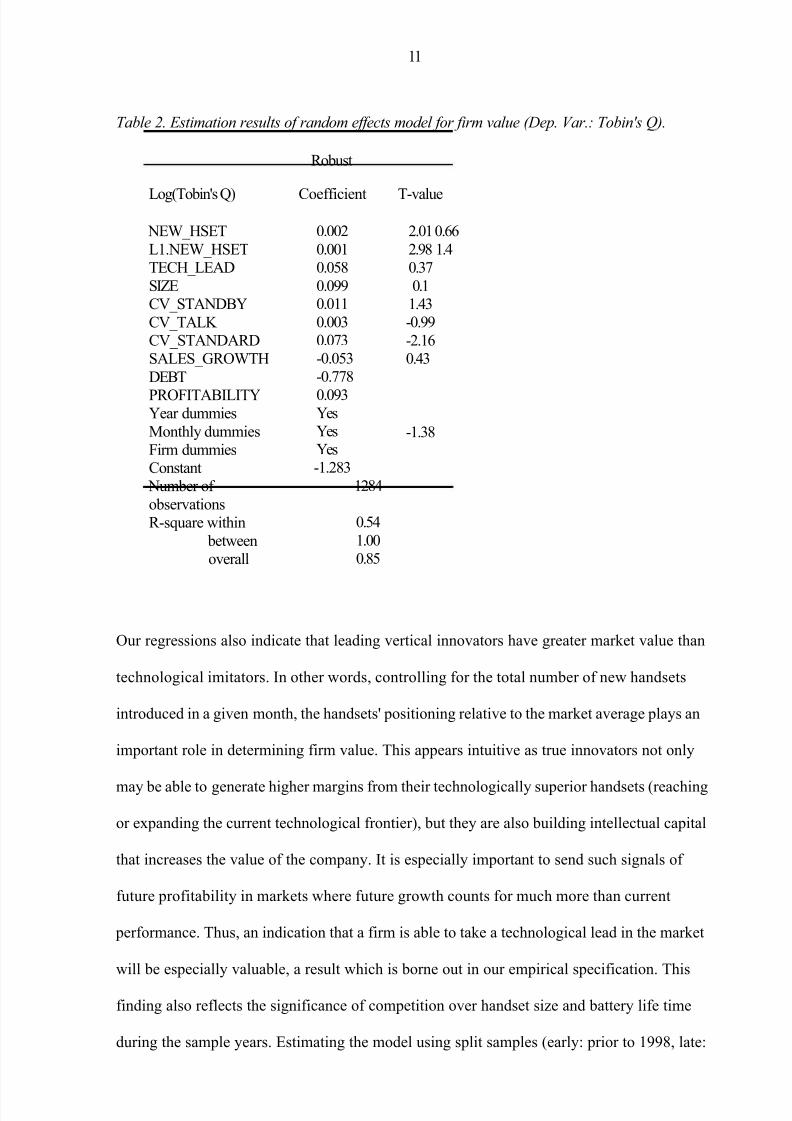
We estimated a random-effects model with standard errors robust to heteroscedasticity and
serial correlation. Our estimated model, reported in Table 2, suggests that the relationship
between the number of new mobile handset models the firm has launched and its market value
is positive and statistically significant. It seems that the market reacts rapidly to the new
handset introductions as only the current month's new products, not the ones launched during
the previous months, matter. That is, the one-period lag of the number of handsets introduced
is insignificant in our regressions.6 This is consistent with the intuition that investors view a
new handset more as an indicator of future innovativeness rather than a proxy for expected
sales in the near future. Another interpretation would be that most sales of new handsets take
place in the first few months after their introduction, which would imply that the model's
success is already well-known shortly after introduction.
8/8/2019 A_study on Mobile Production
http://slidepdf.com/reader/full/astudy-on-mobile-production 16/66
11
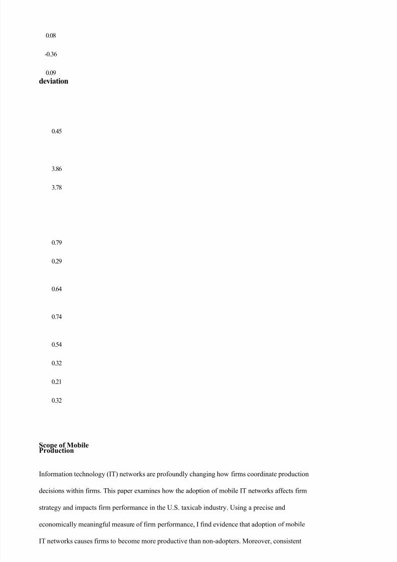
Table 2. Estimation results of random effects model for firm value (Dep. Var.: Tobin's Q).
Robust
Log(Tobin's Q)
NEW_HSETL1.NEW_HSETTECH_LEADSIZECV_STANDBYCV_TALK CV_STANDARDSALES_GROWTHDEBT
PROFITABILITYYear dummiesMonthly dummiesFirm dummiesConstant
Number of observationsR-square within
betweenoverall
Coefficient
0.0020.0010.0580.0990.0110.0030.073-0.053-0.778
0.093YesYesYes-1.283
1284
0.541.000.85
T-value
2.01 0.662.98 1.40.370.1
1.43-0.99-2.160.43
-1.38
Our regressions also indicate that leading vertical innovators have greater market value than
technological imitators. In other words, controlling for the total number of new handsets
introduced in a given month, the handsets' positioning relative to the market average plays an
important role in determining firm value. This appears intuitive as true innovators not only
may be able to generate higher margins from their technologically superior handsets (reaching
or expanding the current technological frontier), but they are also building intellectual capital
that increases the value of the company. It is especially important to send such signals of
future profitability in markets where future growth counts for much more than current
performance. Thus, an indication that a firm is able to take a technological lead in the market
will be especially valuable, a result which is borne out in our empirical specification. This
finding also reflects the significance of competition over handset size and battery life time

8/8/2019 A_study on Mobile Production
http://slidepdf.com/reader/full/astudy-on-mobile-production 17/66
12
1998 and after) shows that the variable TECH_LEAD is highly statistically significant in the
early sample while it does not explain variation in firm value significantly later in the
industry. This suggests that the competitive advantage that cellular manufacturers have
derived from the technological leadership in terms of handset size, talk and standby times had
vanished by the late 1990s, and the firms thereafter needed to employ other, more horizontally
oriented, innovation strategies. This is in line with the observations in Koski and Kretschmer
(2007), who find a shift from vertical to horizontal innovation strategies around that time. 7
The results above shed some light on why this was the case.
Differences in the firms' horizontal innovation and product mix strategies do not, however,
explain the variation in firm values significantly. Note that imitation in the handset production
is substantial: innovative and successful handset features are copied rapidly by the
competitors, reducing returns from such horizontal innovation efforts. This could be one of
the reasons why the coefficients on CV_STANDBY and CV_TALK are not statistically
significant - in other words, a heterogeneous product portfolio is no indication that the firm
will be able to occupy a profitable market niche for long as it is likely to be imitated quickly.
It is also possible that these variables measure firms' product differentiation strategies too
imprecisely. More accurate information on the firms' horizontal innovation choices would be
needed for making general conclusions on the relationship between firm value and its
horizontal innovation strategies. We leave this interesting extension for future work.
7 This is also consistent with Adner and Zemsky (2006) stating that in mature markets when technological

8/8/2019 A_study on Mobile Production
http://slidepdf.com/reader/full/astudy-on-mobile-production 18/66
quality is already relatively high, users' marginal utilities from technological improvements decrease and firms' profits from vertical innovation shrink.

8/8/2019 A_study on Mobile Production
http://slidepdf.com/reader/full/astudy-on-mobile-production 19/66
16
Appendix 1. Description of the data
Manufacturers included in the sample:
Nokia; Ericsson; Motorola; Alcatel; Fujitsu; Hyundai; JRC; Maxon; Mitsubishi;
NEC; Philips; Samsung; Sanyo; Sharp; Toshiba; Sony.
Description of the variables:
Standard
Description of variable
Dependent variable:
(common shares outstanding * prices + book value total assets - common equity) / book value total assets
Explanatory variables:
Log Number of new mobile handsets firm has introduced during the current month.
Log Number of new mobile handsets firm hasintroduced during the previous month.
The sum of three dummy variables that getvalue 1 if handset models firm has introduced during sample year: i) have greater talk time,ii) have greater standby time and iii) arelighter, on average, than all handset models introduced during the year, and 0 otherwise.Log average size of new handset modelsfirm has launched during the year.
Log coefficient of variation of standby time of new handset models firm has launched during the year.
Log coefficient of variation of talk time of newhandset models firm has launched during the year.
Log number of new handset models using
different standards firm has launched during the year.(Sales at year t-Sales at year (t-1))/Sales atyear (t-1)(Total Assets - Total Equity) / Total Assets,annual data
Firm's net income divided by its sales, annualdata
Variable name
TOBINSQ

8/8/2019 A_study on Mobile Production
http://slidepdf.com/reader/full/astudy-on-mobile-production 20/66
NEW_HSET
L1.NEW_HSET
TECH_LEAD
SIZE
CV_STANDBY
CV_TALK
STANDARD
SALES_GROWTH
DEBT
PROFITABILITYMean
0.40
-3.57
-4.02
1.57
11.87
-0.97
-1.26
8/8/2019 A_study on Mobile Production
http://slidepdf.com/reader/full/astudy-on-mobile-production 21/66
0.08
-0.36
0.09
deviation
0.45
3.86
3.78
0.79
0.29
0.64
0.74
0.54
0.32
0.21
0.32
Scope of MobileProduction
Information technology (IT) networks are profoundly changing how firms coordinate production
decisions within firms. This paper examines how the adoption of mobile IT networks affects firm
strategy and impacts firm performance in the U.S. taxicab industry. Using a precise and
8/8/2019 A_study on Mobile Production
http://slidepdf.com/reader/full/astudy-on-mobile-production 22/66
with the predictions of transaction cost economics (Williamson 1975 and 1985), firms respond to
adoption of mobile IT networks by changing their organizational structure, shifting toward
owning a greater fraction of vehicles in their fleets (as opposed to contracting with independent
driver-owners for vehicles). The results suggest that adoption of mobile IT networks increases
asset utilization by improving within-firm coordination but that firms must simultaneously shift
toward a more highly vertically integrated structure to fully capture the benefits of mobile IT
networks, although I cannot formally reject the null hypothesis that the asset utilization and asset
ownership effects operate independently.
This paper addresses endogeneity issues in the relationship between adoption of mobile IT
networks, firm productivity and asset ownership in two important ways. First, by linking mobile
IT network adoption directly to firms, empirical tests that focus on within-firm changes in
productivity and the boundary of the firm control for unobserved time-invariant characteristics of
firms that may bias cross-sectional results. Second, because U.S. taxicab markets are
geographically isolated from one another this paper essentially examines one-hundred and fifty
distinct local markets. I exploit the exogenous variation in local market conditions using an
instrumental variables approach to control for unobservable characteristics of firms that may be
correlated with both adoption and productivity and/or the boundary of the firm. The instrument I
deploy for adoption is lagged average fleet size of other fleets in the same market. The effect of
2

8/8/2019 A_study on Mobile Production
http://slidepdf.com/reader/full/astudy-on-mobile-production 23/66
lagged size of other fleets in the same market should be orthogonal to changes in "own" firm
boundaries and productivity. However, lagged average fleet size may be correlated with adoption
to the extent that markets with larger average fleet size are the kinds of markets where adoption is
more likely to be prevalent.
I find strong evidence that adoption leads to higher rates of fleet ownership of vehicles and
increases firm productivity. The results are consistent with transaction cost economics and
suggest that there are complementarities between the adoption of mobile IT networks and fleet
ownership of vehicles.
The rest of this document is organized as follows:
Section 2 explores the conceptual foundation for this paper and describes the related literature.
Section 3 describes the institutional context in which mobile IT networks are used in the U.S.
taxicab market. Section 4 develops explicit adoption and productivity hypotheses. Section 5
describes the data and the empirical strategy. Section 6 discusses the results. Section 7
concludes.
2. Conceptual framework and related literature
Mobile information technology networks are fundamentally altering how firms organize
production. Given the rapid growth of mobile IT networks in the modern economy, gaining a
deeper understanding of the relationship between the adoption of mobile IT networks, firm
strategy and performance is of great importance. To address these questions the paper builds on
and integrates contract theory and the empirical literatures on information technology and firm
boundaries.
3
8/8/2019 A_study on Mobile Production
http://slidepdf.com/reader/full/astudy-on-mobile-production 24/66
Understanding patterns of asset ownership has been a central issue in organizational economics
since Coase (1937), who argued that firms should coordinate transactions internally only when
doing so is more efficient than coordinating those activities through markets. Contract theorists
extended and refined Coase's insight by highlighting the importance of contractual
incompleteness in the presence of potential opportunism, in particular the problem of hold-up
with respect to firm specific investments, in drawing the boundary of the firm (Williamson 1975,
1985; Klein, Crawford and Alchian 1978). When taxi fleets implement mobile IT networks they
force independent owner-drivers, who could formerly contract with the fleet for generalized
radio-based dispatching services, to choose between being excluded from the fleet's network or
adopting specialized on board computers (OBC). OBC are usually incompatible with other
fleets' dispatching systems and therefore cannot be easily redeployed. Thus, following the
adoption of a mobile IT network, fleets and their pool of potential driver-owners face a joint
investment decision over OBC that has the potential to fundamentally change their contracting
relationship. As predicted by contract theory, which emphasizes the role of asset specificity in
the vertical integration decision, adoption of mobile IT networks leads to a shift in the boundary
of the firm toward fleet ownership of vehicles as fleets acquire independent owner-operators who
do not wish to invest in OBC as non-integrated agents of the fleet.
While there are alternative theoretical lenses through which to view boundary of the firm
questions besides transaction cost economics, the issues of incomplete contracting, hold-up and
asset specificity are particularly salient in this context. Indeed, one of the contributions of this
paper is its sharp theoretical focus on the role of transaction cost economics in the context of
technological change. Given our expectation that mobile IT networks increase the efficiency of
coordinating a network of distributed assets, and the fact that adoption of OBC is a firm-specific
investment that cannot be easily redeployed to another firms mobile IT network, transaction cost
4

8/8/2019 A_study on Mobile Production
http://slidepdf.com/reader/full/astudy-on-mobile-production 25/66
economics should particularly well suited to render predictions about the effect of adoption on the
boundary of the firm. By contrast, agency theory and the property-right theory of the firm rely on
variation in incentives between employees and contractors (Grossman and Hart 1986), a notion
that seems far less germane in an industry where high-powered incentives are nearly ubiquitous
across ownership states. Since most taxi drivers are full residual claimants there is little room to
consider the incentive changing effects of investments in mobile IT networks in taxicab fleets.
By integrating technological change into a transaction cost economics framework the paper builds
on and extends the literature on information technology and firm strategy. While the theoretical
implications of mobile IT networks on the boundary of the firm are relatively straightforward in
this context, examining the empirical relationship between investments in mobile IT networks
and firm strategy from a transaction cost economics perspective is an important step in
developing our understanding of the strategic implications of mobile IT networks specifically and
coordination technologies more generally. In a recent paper, Bartel, Ichniowski and Shaw (2005)
find evidence that adoption of stand-alone information technology changes the organization of
production in valve manufacturing firms. This paper considers similar questions but differs from
theirs in that I consider the impact of the adoption of mobile IT networks on firm strategy and
performance.
The two papers most closely related to this work, Hubbard (2003) and Baker and Hubbard (2003)
study of the effect of OBC adoption on truck utilization and the boundary of trucking fleets.
Hubbard (2003) finds evidence that OBC improves asset utilization and Baker and Hubbard
(2003) find that incentive-improving features of OBC push the boundary of the firm toward
driver-owned vehicles, while coordination-improving features of OBC pull the boundary of the
firm back toward fleet-ownership. However, Baker and Hubbard (2003) could not link OBC
adoption to fleets and therefore could not control for omitted variables that affect both the
5

8/8/2019 A_study on Mobile Production
http://slidepdf.com/reader/full/astudy-on-mobile-production 26/66
technology adoption decision and the boundary of the firm. This paper builds on Hubbard (2003)
and Baker and Hubbard (2003) by examining within-firm changes in performance and the
boundary of the firm, following the adoption of mobile IT networks. This distinction is important
because unobserved heterogeneity amongst adopting and non-adopting biases cross-sectional
analyses. By examining changes in productivity and the boundary of the firm within-firm, the
empirical design controls for time-invariant characteristics of firms which may affect both
adoption and performance and/or boundary of the firm decisions. I explicitly control for
unobservable characteristics of firms that may bias the results using an instrumental variables
(IV) approach that exploits the exogenous characteristics of the local markets in which taxicab
fleets operate.
3. Institutional context
Taxi fleets began using computers during the 1970s, but fully automated data dispatch systems
did not arrive until the early 1980s. Even then adoption of mobile IT networks, comprised of a
central coordination and communication technology and specialized vehicle-level on-board
computers, was limited to a handful of firms until the early to mid-1990s. These systems use a
mobile data terminal installed in each vehicle. Basic mobile IT networks systems called "partially
automated" systems require drivers to indicate their location by entering a zone number into the
terminal and transmitting it to the computer, which organizes vehicles into queues for each zone.
When a customer requests a ride, the computer determines the caller location using a built-in
street directory and sends a message to a central dispatcher. More advanced systems called "fully
automated" systems deploy in-car devices with two-way communication capability, allowing the
back-end optimization algorithm to communicate directly with vehicles. These systems also
automatically monitor pickup and drop-off actions, such as turning the meter on and off. The
6

8/8/2019 A_study on Mobile Production
http://slidepdf.com/reader/full/astudy-on-mobile-production 27/66
most advanced mobile IT networks are GPS-based, which eliminates the need for drivers to enter
zone numbers and tracks a vehicle's exact location at all times.
Computerized dispatch greatly simplifies the coordination of large taxicab fleets. It can also end
claims of dispatcher favoritism by drivers, end call stealing by other cab companies using radio
scanners, and can simplify communication between dispatchers and foreign-born drivers.
However, non-GPS-based systems do not verify the location of a cab and cannot prevent drivers
from manipulating the dispatch system by misrepresenting their current status or location.
Nevertheless, a 1993 case study of 16 fleets with an average of 300 cabs documented 50 to 60
percent reductions in dispatch time at an average cost of $1 million (Gilbert, Nalevanko and
Stone, 1993). More advanced systems rely on in-car terminals with two-way communication
ability. These in-car terminals are three to four times as expensive as one-way communication
terminals. By contrast the back-end computing cost for a fully-automated system is only 50%-
100% more expensive than the back-end computing cost for a partially automated system. Thus,
economies of scale in purchasing are actually steeper for partially-automated systems than for
fully-automated and GPS systems.
Besides strategic issues, local regulatory, competitive and unique geographic factors can
influence the costs and benefits of installing computerized dispatching. Most of these factors are
exogenous to the choices of taxi fleet operators and provide the natural experiment missing from
many studies of technology adoption. Local regulations1 can set retail prices, fix the number of
permits or medallions, devise a permit allocation system (e.g., lottery or auction), set limits on the
transferability of permits, set restrictions on the entry and exit of fleets and may require either
fleets or individuals to own operating permits. Differences between cities, such as regulated fare
1 Taxi regulation is usually promulgated at the city level. As of 1997 seven states used a uniform code to
regulate taxis: Arkansas, Connecticut, Colorado, Delaware, Kentucky, New Mexico, Rhode Island.Kentucky has subsequently changed to city-level regulation.
7

8/8/2019 A_study on Mobile Production
http://slidepdf.com/reader/full/astudy-on-mobile-production 28/66

8/8/2019 A_study on Mobile Production
http://slidepdf.com/reader/full/astudy-on-mobile-production 29/66
changes, may also influence the adoption of automated dispatch systems by changing the benefits
of adoption. Moreover, the unique geography of a city can influence the distribution of rides
between dispatched fares and curbside hails. The paper exploits this natural variation in markets
by using market-level instrumental variables to control for the endogenous nature of the adoption
decision.
4. Hypotheses
The first hypothesis is derived directly from transaction cost economics' emphasis on hold-up and
incomplete contracts, proposing that adoption of mobile IT networks leads to changes in the
boundary of the firm toward more fleet ownership of networked assets:
(H1) Adoption of mobile IT networks should lead to an increase in the fraction of
vehicles that are owned by the fleet relative to those owned by drivers but
operated by the fleet.
The "productivity paradox" in information technology (IT), the dearth of causal evidence
connecting IT adoption and productivity, has been addressed empirically in a number of recent
papers (Brynjolfsson and Hitt 1996, 2003; Hubbard 2003; Bartel, Ichniowski and Shaw 2005).
However, only Athey and Stern (2002) have done so convincingly using mobile IT networks
rather than traditional stand-alone IT. But mobile IT networks are unique and important in their
own right, particularly because they directly shift the returns to activities that require
coordination.2 Because mobile IT networks improve coordination by bringing information to
2 Baker and Hubbard (2003) point out that mobile IT networks can also have monitoring benefits.
However, in this empirical context monitoring is far less important to taxicab fleets because driverstypically have very high powered incentives (e.g., they are full residual claimants) whether they own the
8

8/8/2019 A_study on Mobile Production
http://slidepdf.com/reader/full/astudy-on-mobile-production 30/66

8/8/2019 A_study on Mobile Production
http://slidepdf.com/reader/full/astudy-on-mobile-production 31/66
bear on resource allocation decisions across a networks of assets, the effect of mobile IT networks
on productivity are fundamentally different from traditional stand-alone IT, which raises the
productivity of isolated assets in ways that do not affect coordination directly. Thus this paper
hypothesizes that there is a causal relationship between mobile IT network adoption and firm
productivity, due to coordination benefits:
(H2) Adoption of a mobile IT network should increase firm productivity.
The relationship between productivity and coordination with respect to mobile IT networks
speaks directly to the importance of assessing the impact of the adoption of mobile IT networks
on productivity in conjunction with considerations of the boundary of the firm. Because contract
theory predicts that adoption of mobile IT networks should exhibit positive dependency with
changes in asset ownership for reasons of efficiency, this setting is a natural place to consider the
empirical evidence in support of complementarities in the production function, in the sense of
Milgrom and Roberts (1990). I expect that the marginal effect of mobile IT network adoption on
productivity should be higher in the presence of larger shifts in the boundary of the firm toward
centralized ownership:
(H3) The firm's production function should exhibit complementarities between adoption
of mobile IT networks and increasing fleet ownership of vehicles.
While there is broad support for the hypothesis that complementarities between IT and
organizational change are an important part of the productivity equation, there is relatively little
evidence of specific business practices that increase the marginal returns to IT adoption. This
taxicab or lease it from the firm. I shall therefore emphasize the coordination benefits inherent in mobile ITnetworks throughout the paper.
9
8/8/2019 A_study on Mobile Production
http://slidepdf.com/reader/full/astudy-on-mobile-production 32/66
paper examines the complementarities question directly in an industrial context where the
econometrician can directly observe both shifts in asset ownership and changes in productivity.
5. Data and Empirical Design
5.1 Data
The core dataset from this paper comes from the 1992 and 1997 Economic Census of
Transportation and Warehousing firms (ECTW). The ECTW began tracking the private-for-hire
industry in 1992 and has continued to track the industry every five years (2002 data has been
collected but not yet released). The ECTW is a comprehensive dataset that includes every taxi
firm in the United States with at least one employee (SIC code 412100): 3,184 in 1992 and 3,337
in 1997. I augment the standard ECTW data with the accompanying supplementary files on
vehicle inventory and segment revenues. This micro-data is extremely valuable as it includes
firm revenue, line of business revenue, number of taxis by ownership type (e.g., fleet-owned
versus driver owned) and organizational form (e.g., partnership, cooperative etc.) which allows
for a very precise measure of each firm's factor inputs and output. There are approximately 1,000
firms in the 1992 and 1997 ECTW with complete records, which comprise between 60-80% of
the $2 billion PHV industry.3 The ECTW does not, however, contain mobile IT network
adoption information.
To generate the dataset used for this paper I merge technology adoption data from the Transit
Cooperative Research Program (TCRP) and from my own supplemental survey with the ECTW
data. The TCRP survey conducted by the Institute for Transportation Research and Education at
3 1,829 observations in 1992 and 1,719 observations in 1997 are considered incomplete and unusable
because they do not contain the number of taxicabs in their fleet. This set is primarily administrative record(AR) observations - very small firms that the Economic Census does not actually survey but rather imputesvalues for.
10

8/8/2019 A_study on Mobile Production
http://slidepdf.com/reader/full/astudy-on-mobile-production 33/66
8/8/2019 A_study on Mobile Production
http://slidepdf.com/reader/full/astudy-on-mobile-production 34/66
North Carolina State University in conjunction with the International Taxicab and Livery
Association and Multisystems, Inc. A report including summary statistics from the survey was
published in 2002 under the title "TCRP Report 75: The Role of the Private-for-Hire Vehicle
Industry in Public Transit" (1998). A survey questionnaire was mailed to 13,751 private-for-hire
operators (taxi, limousine and other private transportation providers) identified from previous
studies of which 1,691 were returned undeliverable. 677 operators responded to the survey,
representing at least one fleet from each state. 363 taxi fleets completed all the fields of interest
for the analyses in this paper including questions about dispatching technology, and number of
vehicles by ownership type.4 I augmented the TCRP survey with our own survey of the largest
2,000 taxicab operators in the Dun and Bradstreet national database of firms with taxicab SIC
codes (e.g., 412100). 391 surveys were returned undeliverable and 403 firms responded with
complete questionnaires (25% response rate). 272 of the firms that responded to the authors'
survey began operations before 1997. I merged the 635 (363 TCRP observations and 272 author
survey observations) technology observations with the 3,153 observations in the 1997 ECTW by
zip code or county and firm size and generated 409 complete observations.5 Of these 409
observations 532 were in both the 1992 and 1997 ECTW.
See Table 1 for summary statistics and Table 2 for correlations between key variables. It is
interesting to note in Table 1 that the secular shift in the industry is away from fleet ownership of
taxis toward driver ownership of taxis. Yet I predict the opposite in mobile information
technology adopters, expecting a shift toward fleet ownership in these firms.
4 I are grateful to Tom Cook and Gorman Gilbert for generously sharing the detailed responses to the TCRP
survey with us.5 The 226 unmatched observations were primarily very small firms that could not be matched preciselywhere there were multiple small fleets within a market and fleets that are in the technology survey data set but failed to report line of business revenue in the ECTW.
11

8/8/2019 A_study on Mobile Production
http://slidepdf.com/reader/full/astudy-on-mobile-production 35/66

8/8/2019 A_study on Mobile Production
http://slidepdf.com/reader/full/astudy-on-mobile-production 36/66
In addition to the quantitative data, I conducted 73 semi-structured interviews with city taxi
regulators (37), fleet owners and mobile IT network technology vendors (26) and taxi drivers (10)
focusing on the relationship between regulatory change, lateral entry and driver ownership.
These interviews provided a wealth of insights and anecdotes that greatly facilitated hypothesis
development for this paper.6
One of the key advantages of studying the taxicab industry is that it is comprised of hundreds of
distinct independent local markets. The ECTW contains geographic information about firm
location at the level of zip code, which allows us to take advantage of this natural source of
variation in the industry. To do so, I attach additional geographic information such as population
density, income per capita and regulatory information; group firms into markets; and create
market-level variables that allow us to exploit the high degree of cross-sectional variation in the
data by market.
A second important advantage of the taxi industry is that taxi prices are set by local regulation in
every major market. This means that productivity regressions with market-level fixed effects
capture differences in physical output per unit of input across firms rather than relying simply on
revenue measures of output as most productivity studies do. A number of papers have
demonstrated the perils of relying on deflated revenues to measure total factor productivity (TFP)
including Klette and Griliches (1996), Katayama, Lu and Tybout (2003) and most recently Foster,
Halitwanger and Syverson (2005), hereafter FHS, who find that prices and technical efficiency
6 I are indebted to C.J. Christina (New Orleans, LA), Jason Diaz CEO of Taxipass (New York, NY),
Thomas Drischler (Los Angeles, CA), John Hamilton (Portland, OR), Stan Faulwetter (San Jose, CA),Alfred La Gasse Executive Vice President of the Taxi Limousine and Paratransit Association (TLPA),Kimberly Lewis (Washington, D.C.) Joe Morra (Miami, FL), Marco Henry, President of Yellow Cab(Bloomfield, CT), John Perry (Mentor Engineering), David Reno (Boston, MA), Aubby Sherman (Detroit,MI), Doug Summers (Digital Dispatch Systems) and especially Craig Leisy (Seattle, WA) for so freelysharing with us the wealth of knowledge they have accumulated regarding the U.S. taxicab industry. I alsowish to thank the hundreds of taxi company executives who responded to our written mail survey and toour requests for interviews at the TLPA conference in Boston, MA in 2006. I acknowledge excellentassistance from YooMin Hong, Elisa Wong and especially Stephanie Simos in conducting survey research.
12

8/8/2019 A_study on Mobile Production
http://slidepdf.com/reader/full/astudy-on-mobile-production 37/66

8/8/2019 A_study on Mobile Production
http://slidepdf.com/reader/full/astudy-on-mobile-production 38/66
tend to be inversely correlated. They conclude that, "previous work linking (revenue-based)
productivity to survival has confounded the separate and opposing effects of technical efficiency
and demand," an issue which this paper squarely addresses. FHS call physical output measures
of technical efficiency TFPQ to differentiate it from traditional measures of TFP. This paper
follows their notation by using TFPQ to represent the technical efficiency of the firm.
Empirical tests are supported by the relatively simple and homogenous production function in the
taxicab industry, since simple production functions control for heterogeneous influences on
factors of production and allow the econometrician to isolate the effects of unobserved
organizational characteristics on observed productivity. This approach minimizes measurement
error in the key reduced-form establishment-level productivity measure I employ, total factor
productivity in quantities (TFPQ).
Following the standard approach for measuring plant (e.g., fleet) total factor productivity in
quantities (TFPQ) for firm i at time t is computed as the log of its physical output q minus a
weighted sum of its logged capital k and labor l inputs. That is,
(1) TFPQit = qit - α ktk it -α ltlit
The key feature of (1) is that output is measured in physical units, rather than in dollars. When
output is measured in dollars rather than in physical units, TFP measures are contaminated by
price differences across firms. In this dataset we do not observe physical outputs or market
prices, only revenues in dollars. However, we can easily recover TFPQ as a measure of physical
output in this case by including a market fixed effect in a standard Cobb-Douglas production
function, because market prices are fixed for all firms in a market. Market fixed effects have the
added advantage of eliminating unobservable market level characteristics that influence returns. I
13
8/8/2019 A_study on Mobile Production
http://slidepdf.com/reader/full/astudy-on-mobile-production 39/66
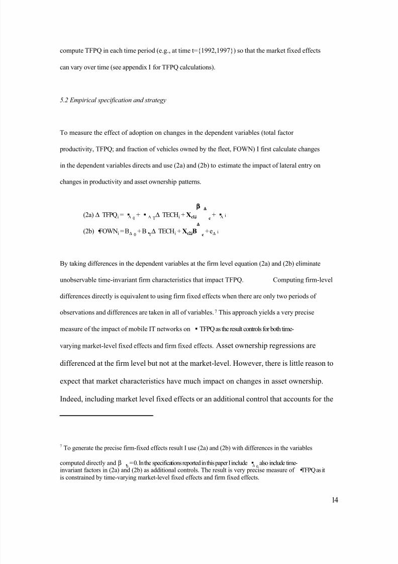
compute TFPQ in each time period (e.g., at time t={1992,1997}) so that the market fixed effects
can vary over time (see appendix I for TFPQ calculations).
5.2 Empirical specification and strategy
To measure the effect of adoption on changes in the dependent variables (total factor
productivity, TFPQ; and fraction of vehicles owned by the fleet, FOWN) I first calculate changes
in the dependent variables directs and use (2a) and (2b) to estimate the impact of lateral entry on
changes in productivity and asset ownership patterns.
(2a) ∆ TFPQi =∆ 0+∆ T
∆ TECHi + Xc1,iβ ∆ c+∆ i
(2b)FOWNi = B∆ 0+ BT∆ TECHi + Xc2,iB∆ c
+ e∆ i
By taking differences in the dependent variables at the firm level equation (2a) and (2b) eliminate
unobservable time-invariant firm characteristics that impact TFPQ. Computing firm-level
differences directly is equivalent to using firm fixed effects when there are only two periods of
observations and differences are taken in all of variables.7 This approach yields a very precise
measure of the impact of mobile IT networks onTFPQ as the result controls for both time-
varying market-level fixed effects and firm fixed effects. Asset ownership regressions are
differenced at the firm level but not at the market-level. However, there is little reason to
expect that market characteristics have much impact on changes in asset ownership.
Indeed, including market level fixed effects or an additional control that accounts for the
7 To generate the precise firm-fixed effects result I use (2a) and (2b) with differences in the variables
computed directly and β0
= 0. In the specifications reported in this paper I include∆ 0also include time-
invariant factors in (2a) and (2b) as additional controls. The result is very precise measure of TFPQ as itis constrained by time-varying market-level fixed effects and firm fixed effects.
14

8/8/2019 A_study on Mobile Production
http://slidepdf.com/reader/full/astudy-on-mobile-production 40/66
8/8/2019 A_study on Mobile Production
http://slidepdf.com/reader/full/astudy-on-mobile-production 41/66
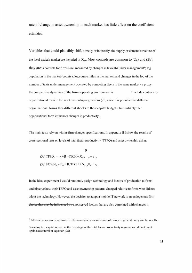
rate of change in asset ownership in each market has little effect on the coefficient
estimates.
Variables that could plausibly shift, directly or indirectly, the supply or demand structure of
the local taxicab market are included in Xc,i. Most controls are common to (2a) and (2b),
they are: a controls for firms size, measured by changes in taxicabs under management8; log
population in the market (county); log square miles in the market; and changes in the log of the
number of taxis under management operated by competing fleets in the same market - a proxy
the competitive dynamics of the firm's operating environment is. I include controls for
organizational form in the asset ownership regressions (2b) since it is possible that different
organizational forms face different shocks to their capital budgets, but unlikely that
organizational form influences changes in productivity.
The main tests rely on within-firm changes specifications. In appendix II I show the results of
cross-sectional tests on levels of total factor productivity (TFPQ) and asset ownership using:
(3a) TFPQit =0 + β TTECH + Xc1,itβ c + ε it
(3b) FOWNit = B0 + BTTECH + Xc2,itBc + eit
In the ideal experiment I would randomly assign technology and factors of production to firms
and observe how their TFPQ and asset ownership patterns changed relative to firms who did not
adopt the technology. However, the decision to adopt a mobile IT network is an endogenous firm
choice that may be influenced by unobserved factors that are also correlated with changes in
8 Alternative measures of firm size like non-parametric measures of firm size generate very similar results.
Since log taxi capital is used in the first stage of the total factor productivity regressions I do not use itagain as a control in equation (2a).
15

8/8/2019 A_study on Mobile Production
http://slidepdf.com/reader/full/astudy-on-mobile-production 42/66

8/8/2019 A_study on Mobile Production
http://slidepdf.com/reader/full/astudy-on-mobile-production 43/66
TFPQ and asset ownership. I address the potential for selection bias in the technology adoption
decision using an instrumental variables (IV) approach that exploits the high degree of variation
in market characteristics in which taxi fleets operate. Specifically, I use lagged (e.g., 1992)
average fleet size for other firms in the same market as an instrument for adoption.
Lagged size of other fleets in the same market should not cause "own firm" to adopt a mobile IT
network or cause changes in "own firm" productivity or asset ownership. However, lagged
average size of other fleets in the same market may be correlated with "own firm" adoption to the
extent that "own firm" is operating in a market where exogenous characteristics of the market
necessitate that firms are large on average and therefore tend to exhibit high demand for
coordination. One might also expect that knowledge spillovers associated with operating in a
market where other firms adopt mobile IT networks influence "own firm" adoption since "own
firm" is more likely to be exposed to the benefits of mobile IT networks when their (large)
competitors adopt it. Therefore, lagged average size of other firms in the same market should
only be expected to have an effect on changes in "own firm" through its effect on "own firm"
adoption of mobile IT networks.
6. Results and Analysis
The central tests of the first hypothesis are within-firm regressions on changes in the boundary of
the firm following the adoption of mobile IT networks. Table 3 shows the results of the tests of
this hypothesis. Column (1) demonstrates a strong unconditional correlation between adoption
and increases in the fraction of vehicles that are fleet owned on the order of 15%. This result was
replicated using firm fixed effects and a time dummy. The results are much larger (55%) when I
instrument for adoption using lagged (e.g., 1992) average fleet size of other firms in the same
market suggesting that true impact of mobile IT network adoption on the boundary of the firm is
16

8/8/2019 A_study on Mobile Production
http://slidepdf.com/reader/full/astudy-on-mobile-production 44/66

8/8/2019 A_study on Mobile Production
http://slidepdf.com/reader/full/astudy-on-mobile-production 45/66
17

8/8/2019 A_study on Mobile Production
http://slidepdf.com/reader/full/astudy-on-mobile-production 46/66
evidence presented in this paper, strongly suggests that vehicles with OBC are more valuable than
those without, the budget constraints hypothesis is plausible. Although I use organizational form
(cooperative, partnership and sole proprietorship) to proxy for budget constraints faced by the
firm, the baseline tests do not account for budget constraints faced by drivers. I consider this
alternative hypothesis by testing whether adopting fleets acquire more vehicles from independent
drivers in markets where drivers are more likely to be financially constrained. Specifically, I use
population density as a proxy for wealth constraints and then test to see if the interaction between
adoption and population density impacts firm boundaries. Since permit prices should be
correlated with population density, the cost of OBC should have a smaller marginal impact on a
driver's resources in high density markets. To test the effect of driver budget constraints on
changes in the boundary of the firm I simply add the term DENSITY x TECH to the regression in
column (4). The coefficient on DENSITY x TECH operates in the direction expected but the
effect is small (0.004 per 1,000 people per square mile) and insignificant (t=0.23), providing no
evidence that wealth constraints have a significant impact on the change in firm boundaries.
Table 4 shows the main tests of the second hypothesis that adoption of mobile IT networks leads
to improved productivity (TFPQ). Column (1) shows an economically meaningful and
statistically significant correlation between adoption and changes in productivity suggesting
adoption leads to a 15% improvement in productivity. I interpret changes in productivity in terms
of real output per unit of input. In other words the adoption of mobile IT networks is correlated
with as a 15% increase in ride-miles per taxicab. Of course, it is unlikely that firms would adopt
mobile IT networks if they did not lead to increased levels of productivity so this result is hardly
surprising. However, this same logic points out how difficult it is to interpret OLS coefficients as
the causal effect of adoption on changes in productivity. Since unobserved heterogeneity in the
usefulness of mobile IT networks to firms implies that only the firms most likely to benefit from
18

8/8/2019 A_study on Mobile Production
http://slidepdf.com/reader/full/astudy-on-mobile-production 47/66
the mobile IT networks are likely to adopt it. Therefore, I instrument for technology adoption
using a 2SLS approach.
The point estimates are twice as large when I instrument for adoption in column (2), although the
result is not statistically different from the OLS point estimate. Column (2) can be interpreted as
showing that adoption of mobile IT networks causes taxicab ride-miles to increase by 33%
relative to taxicabs in fleets that do not adopt mobile IT networks, although the standard error is
much larger than in the univariate OLS regression in column (1).
Adding controls to the OLS regression (column 3) improves the precision of the estimate and
increases the estimated magnitude of the effect to 20%. IV estimates of the effect of adoption on
productivity conditional on the vector of controls are similar in magnitude to the unconditional
estimates in column (2), although the result is on the margin of statistical significance. These
results support the hypothesis that adoption of mobile IT networks increases firm productivity by
improving asset utilization.
Taken together, Tables 3 and 4 provide evidence that adoption of mobile IT networks
simultaneously leads to increased firm productivity and causes the boundary of the firm to shift
toward vertical integration to allow firms to more fully capture the coordination benefits
associated with the technology. I formally test for the existence of complementarities in the
production function in Table 5 by interacting the change in the fraction of vehicles owned by the
firm with adoption of mobile IT networks. In each of the specifications (with or without controls,
on or off the common support of the distribution of firms that adopt or do not adopt mobile IT
networks) I find no evidence of first-order complementarities in the production function. The
point estimate on the interaction term cannot be measured reliably, and in the preferred
specification the sign on the interaction term is negative, although it usually statistically
19
8/8/2019 A_study on Mobile Production
http://slidepdf.com/reader/full/astudy-on-mobile-production 48/66
insignificant or on the margin of significance. Alternative specifications flip the sign on the
interaction term so that it operates in the direction expected but the result is never precisely
estimated and (obviously) not robust to specification. Thus, I cannot reject that the adoption of
mobile IT networks independently increases firm productivity and shift the boundary of the firm
toward firm ownership of vehicles.
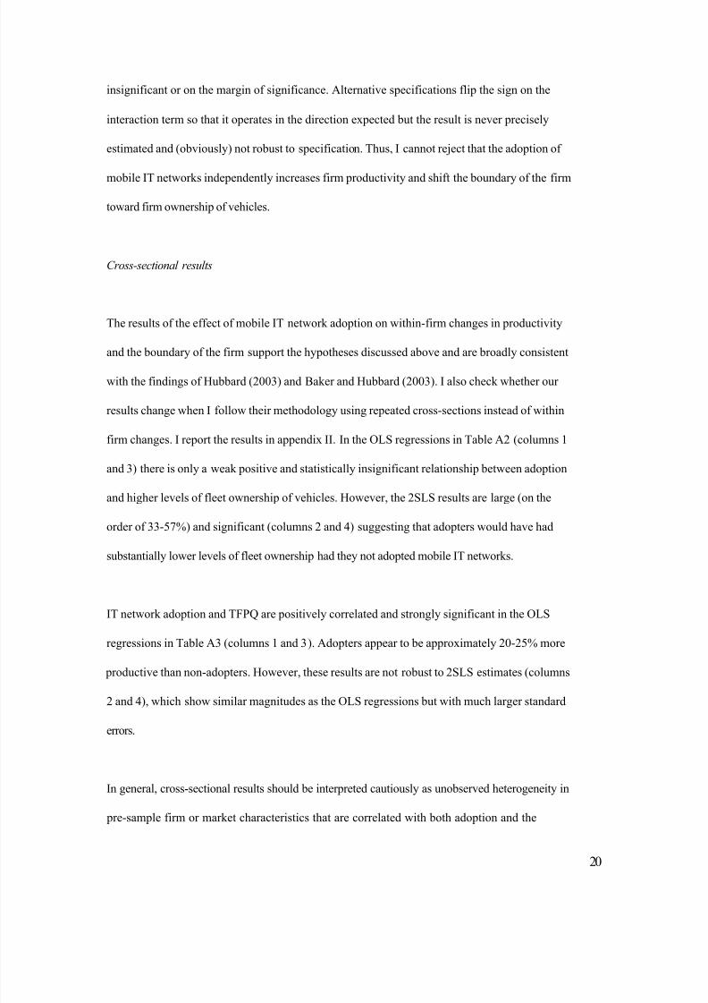
Cross-sectional results
The results of the effect of mobile IT network adoption on within-firm changes in productivity
and the boundary of the firm support the hypotheses discussed above and are broadly consistent
with the findings of Hubbard (2003) and Baker and Hubbard (2003). I also check whether our
results change when I follow their methodology using repeated cross-sections instead of within
firm changes. I report the results in appendix II. In the OLS regressions in Table A2 (columns 1
and 3) there is only a weak positive and statistically insignificant relationship between adoption
and higher levels of fleet ownership of vehicles. However, the 2SLS results are large (on the
order of 33-57%) and significant (columns 2 and 4) suggesting that adopters would have had
substantially lower levels of fleet ownership had they not adopted mobile IT networks.
IT network adoption and TFPQ are positively correlated and strongly significant in the OLS
regressions in Table A3 (columns 1 and 3). Adopters appear to be approximately 20-25% more
productive than non-adopters. However, these results are not robust to 2SLS estimates (columns
2 and 4), which show similar magnitudes as the OLS regressions but with much larger standard
errors.
In general, cross-sectional results should be interpreted cautiously as unobserved heterogeneity in
pre-sample firm or market characteristics that are correlated with both adoption and the
20

8/8/2019 A_study on Mobile Production
http://slidepdf.com/reader/full/astudy-on-mobile-production 49/66
dependent variables of interest could bias the coefficient estimates. In this context, using lagged
market-level instruments, the 2SLS cross-sectional results are broadly consistent with the 2SLS
results of the regressions on within-firm changes. This implies that the effect of unobserved
within-firm variation on the observed relationship between adoption and higher levels of TFPQ
and fleet ownership of vehicles is not particularly important in this context, suggesting that
lagged market-level instruments are sufficient to identify the effects of interest even in cross-
section.
7. Conclusion
This central proposition of this paper is that the adoption of mobile IT networks leads to
improved performance through improved coordination and increased vertical integration for
transaction cost economizing reasons. By adopting mobile IT networks firms can better
coordinate resources within the firm leading to improved asset utilization. By simultaneously
vertically integrating, firms overcome haggling and hold-up costs associated with implementing
mobile IT networks, which allows them to leverage the benefits of the technology across the firm.
Although there is a rich theoretical basis for expecting such effects there has been little work
testing these propositions empirically in the context of coordination technologies. This paper
identifies within-firm effects of mobile IT network adoption on the boundary of the firm and
performance rather than relying on potentially misleading results from repeated cross-sections as
previous empirical work has done. The results suggest that adoption of mobile IT networks
improves firm performance through improved coordination but requires the firm to shift toward
an increasingly vertically integrated structure to fully capture the benefits of mobile IT networks,
although I cannot formally reject the null hypothesis that the asset utilization and asset ownership
effects operate independently.
21

8/8/2019 A_study on Mobile Production
http://slidepdf.com/reader/full/astudy-on-mobile-production 50/66
Bibliography
Athey, Susan and Scott Stern, (1998) "An Empirical Framework for Testing Theories About
Complementarity in Organizational Design" NBER Working Paper 6600.
Athey, Susan and Scott Stern, (2002) "The Impact of Information Technology on Emergency Health
Care Outcomes" Rand Journal of Economics, 33(3): 399-432.
Baker, George F. and Thomas N. Hubbard, (2003) "Make Versus Buy in Trucking: Asset
Ownership, Job Design and Information," American Economic Review: 551-572.
Bartel, Ann P., Casey Ichniowski and Kathryn L. Shaw, (2005) "How Does Information
Technology Really Affect Productivity? Plant-Level Comparisons of Product Innovation,
Process Improvement and Worker Skills," NBER Working Paper #11773.
Brynjolfsson, Erik. and Lauren M. Hitt, (1996) "Paradox Lost? Firm-level evidence on the returns
to information systems spending." Management Science, 42(4):541-558.
Brynjolfsson, Erik and Lauren M. Hitt, (2000) "Beyond Computation: Information Technology,Organizational Transformation and Business Performance," Journal of Economic Perspectives.
Brynjolfsson, E. and Hitt, L., (2003) "Computing Productivity: Firm-Level Evidence," The Review
of Economics and Statistics, 85(4): 793-808.
Coase, Ronald (1937) "The Nature of the Firm," Economica 4: 386-405.
Foster, Lucia, John Haltiwanger, and Chad Syverson (2005) "Reallocation, Firm Turnover, and
Efficiency: Selection on Productivity or Profitability?," Working Paper.
Gilbert, Gorman, Anna. Nalevanko and John R. Stone, (1993) "Computer Dispatch and
Scheduling in the Taxi and Paratransit Industries: An Application of Advanced Publictransportation Systems," ITRE Working Paper.
Grossman, Sanford and Oliver Hart, (1986) "The Costs and Benefits of Ownership: A Theory of
Vertical and Lateral Integration," Journal of Political Economy, Vol. 94, (August): 691-719.
Hubbard, T., (2003) "Information, Decisions, and Productivity: On Board Computers and
Capacity Utilization in Trucking," American Economic Review: 1328-1353.
Katayama, Haijme, Shihua Lu and James Tybout, (2003) "Why Plant-Level Productivity Studies are
Often Misleading, and an Alternative Approach to Inference," NBER Working Paper 9617.
Klein, Benjamin, Robert G. Crawford and Armen A. Alchian, (1978) "Vertical Integration,Appropriable Rents and the Competitive Contracting Process," Journal of Law and Economics 21:
297-326.
Klette, Tor Jakob and Zvi Griliches, (1996) "The Inconsistency of Common Scale Estimators When
Output Prices are Unobserved and Endogenous," Journal of Applied Econometrics 11(4): 343-361.
22

8/8/2019 A_study on Mobile Production
http://slidepdf.com/reader/full/astudy-on-mobile-production 51/66
Milgrom, Paul and John Roberts, (1990) "The Economics of Modern Manufacturing:
Technology, Strategy and Organization," American Economic Review 80 (3): 511-28.
Transit Cooperative Research Program Report 75, (1998) "The Role of the Private-for-Hire
Vehicle Industry in Public Transit."
Stanley, Michael and Raymond J. Burby, (1988) "A Statistical Profile of the Private Taxicab andParatransit Industry," a U.S. Department of Transportation report prepared in conjunction with the
UNC-Chapel Hill Center for Urban and Regional Studies.
Williamson, Oliver, (1975) Markets and Hierarchies: Analysis and Antitrust Implications, New York:
Free Press.
Williamson, Oliver, (1985) The Economic Institutions of Capitalism: Firms, Markets, Relational
Contracting, New York: Free Press.
23

8/8/2019 A_study on Mobile Production
http://slidepdf.com/reader/full/astudy-on-mobile-production 52/66
Table 1 - Descriptive Statistics
Panel A - Unbalanced Panel
1992 1997
Variable N Mean Std dev N Mean Std dev
TFPQ 229 0.64 1.41 409 0.26 0.82
Taxi revenue ($000) 229 1124 2713 409 1146 3147
Total taxis 229 44 93 409 51 107
Taxi capital ($000) 229 585 1355 409 634 1522
Fleet owned taxis 229 37 90 409 32 90
Driver owned taxis 229 7 30 409 19 59
TECH 229 0.00 0.00 409 0.28 0.45
Taxis in the county -i 229 129 340 409 262 512
Average 1992 fleet size - i 229 18 29 409 15 27
County population (000) 229 695 958 409 799 1322
County square miles 229 1054 1878 409 1164 1899
Sole proprietor 229 0.10 0.30 409 0.15 0.36Partnership 229 0.01 0.09 409 0.03 0.18
Cooperative 229 0.05 0.21 409 0.03 0.17
Panel B - Balanced Panel
1992 1997
N Mean Std dev N Mean Std dev
TFPQ 166 0.29 0.71 166 0.39 0.76
Change in TFPQ 166 n/a n/a 166 0.10 0.48
Taxi revenue ($000) 166 1417 3084 166 1855 4564
Total taxis 166 50 103 166 66 123Taxi capital ($000) 166 683 1536 166 923 1995
Fleet owned taxis 166 44 103 166 50 121
Driver owned taxis 166 6 23 166 16 35
Change in fleet owned taxis (%) 166 n/a n/a 166 -0.19 0.45
TECH 166 0.00 0.00 166 0.34 0.48
Taxis in the county -i 166 151 390 166 288 474
Average 1992 fleet size -i 166 20 31 166 20 31
County population (000) 166 711 1065 166 795 1157
County square miles 166 1100 1576 166 1094 1575
Sole proprietor 166 0.09 0.29 166 0.09 0.29
Partnership 166 0.01 0.11 166 0.02 0.13
Cooperative 166 0.04 0.20 166 0.04 0.20
63 firms of the 229 in the 1992 cross-section exited the industry after 1992 leaving 166
observations in the 1992 and 1997 panel. There are 243 entrants (between 1992 and 1997) in the
1997 Unbalanced Panel.
24

8/8/2019 A_study on Mobile Production
http://slidepdf.com/reader/full/astudy-on-mobile-production 53/66
Table 2 - 1997 Balanced Panel Correlations (n=166)
TFPQ ∆ TFPQ Taxi rev. Tot. taxis Taxi K FOWN% ∆ FOWN%
TFPQ 1
∆ TFPQ 0.43 1
Taxi rev. 0.45 0.23 1
Tot. taxis 0.14 0.12 0.65 1Taxi K 0.15 0.16 0.67 0.98 1
FOWN% 0.10 0.25 0.22 0.10 0.21 1
FOWN% 0.13 0.10 0.14 0.05 0.13 0.73 1
TECH 0.17 0.15 0.29 0.36 0.34 0.09 0.16
Fips taxi-i 0.28 0.21 0.50 0.39 0.41 0.19 0.06
Avg. SZ-i 0.09 0.12 0.19 0.18 0.21 0.21 0.22
Fips pop2Fips mi
Sole prop.
P-ship
Coop.
TECH
Fips taxi-i
Avg. SZ-i
0.05
0.37
-0.09
-0.07
0.10
TECH
1
0.00
0.38
0.09
0.13
-0.11
-0.06
0.07
Fips taxi-i
1
0.11
0.32
0.
49
-0.1
0
-0.
04
0.
02
Avg.
SZ-i
1
0.49
0.
08
-0.1
3
-0.
03
-0.
00
Fips pop
0.51
0.1
0
-0.12
-0.0
3
0.0
0
Fips
mi2
0.17
0.11
-0.10
0.02
0.06
Sole prop.
0.11
0.11
-0.13
-0.02
0.00
P-ship
Fips pop2
Fips miSole prop.
P-ship Coop.
0.10
0.04
-0.10
-0.10
0.04
0.67
0.40
-0.09
-0.05
0.08
0.07
0.06
-0.11
-0.04
0.01
1
0.23
-0.15
0.01 0.18
1
0.09
-0.04
0.07
1
-0.03
-0.07
1
-0.03

8/8/2019 A_study on Mobile Production
http://slidepdf.com/reader/full/astudy-on-mobile-production 54/66
25

8/8/2019 A_study on Mobile Production
http://slidepdf.com/reader/full/astudy-on-mobile-production 55/66
Table 3: Adoption of mobile IT networks and the boundary of the firm
Within-firm changes 1992 - 1997
Dependent variable = Change in the fraction of fleet owned taxis (∆ FOWN)
(1) (2) (3) (4)
OLS 2SLS OLS 2SLS
TECH 0.15 ** 0.55 *** 0.19 *** 0.63 ***
(0.07) (0.16) (0.07) (0.16)
Change in taxis -0.01 *** -0.01 ***
(0.00) (0.00)
Sole proprietor -0.19 * -0.15
(0.11) (0.14)
Partnership -0.08 0.07
(0.17) (0.18)
Cooperative -0.06 -0.11
(0.09) (0.13)
Change in log(taxis in the market -i)
Log(population)
Log(square miles)
0
.0
2
(0
.0
2)
0
.0
4
(0
.0
3)0
.0
2
(0
.0
3)
0
.
0
3
(
0
.
0
3
)
0
.
0
3
(
0
.
8/8/2019 A_study on Mobile Production
http://slidepdf.com/reader/full/astudy-on-mobile-production 56/66
03)
0.03
(0.03)
Constant -0.24 *** -0.38 *** -0.81 ** -0.87 **
(0.04) (0.07) (0.36) (0.38)
N 166 166 166 166
R 2 0.02 n/a 0.20 n/a
Standard errors are robust and clustered at the metropolitan statistical area level.
First-state results for regression (2) using lagged (1992) average fleet size in the same market as an
instrument were: IV coefficient 0.006, standard error (0.001). F-stat = 28, Adjusted R 2 = 0.14.
First-state results for regression (4) using lagged (1992) average fleet size in the same market as aninstrument were: IV coefficient 0.005, standard error (0.001). F-stat = 9, Adjusted R 2 = 0.15.
*** Significant at the 1% level, ** Significant at the 5% level, * Significant at the 10% level
26

8/8/2019 A_study on Mobile Production
http://slidepdf.com/reader/full/astudy-on-mobile-production 57/66
Table 4: Adoption of mobile IT networks and productivity
Within-firm changes 1992 - 1997
Dependent variable = Change in TFPQ
(1) (2) (3) (4)
OLS 2SLS OLS 2SLS
TECH 0.15 ** 0.33 ** 0.20 *** 0.31 *
(0.08) (0.16) (0.07) (0.18)
Change total vehicles -0.00 *** -0.00 ***
(0.00) (0.00)
Change in log taxis in the market -i
Log (population)
Log (square miles)
0.01
(0.02)
0.05 ***
(0.01)
0.03
(0.03)
0.01
(0.02)
0.05 ***
(0.01)
0.03
(0.03)
Constant 0.05 -0.01 0.08 0.05
(0.05) (0.07) (0.05) (0.08)
N 166 166 166 166
R 2 0.02 n/a 0.11 n/a
Standard errors are robust and clustered at the metropolitan statistical area level.
First-state results for regression (2) using lagged (1992) average fleet size in the same market as an
instrument were: IV coefficient 0.006, standard error (0.001). F-stat = 28, Adjusted R 2 = 0.14.
First-state results for regression (4) using lagged (1992) average fleet size in the same market as an
instrument were: IV coefficient 0.005, standard error (0.001). F-stat = 9, Adjusted R 2 = 0.15.
*** Significant at the 1% level, ** Significant at the 5% level, * Significant at the 10% level

8/8/2019 A_study on Mobile Production
http://slidepdf.com/reader/full/astudy-on-mobile-production 58/66
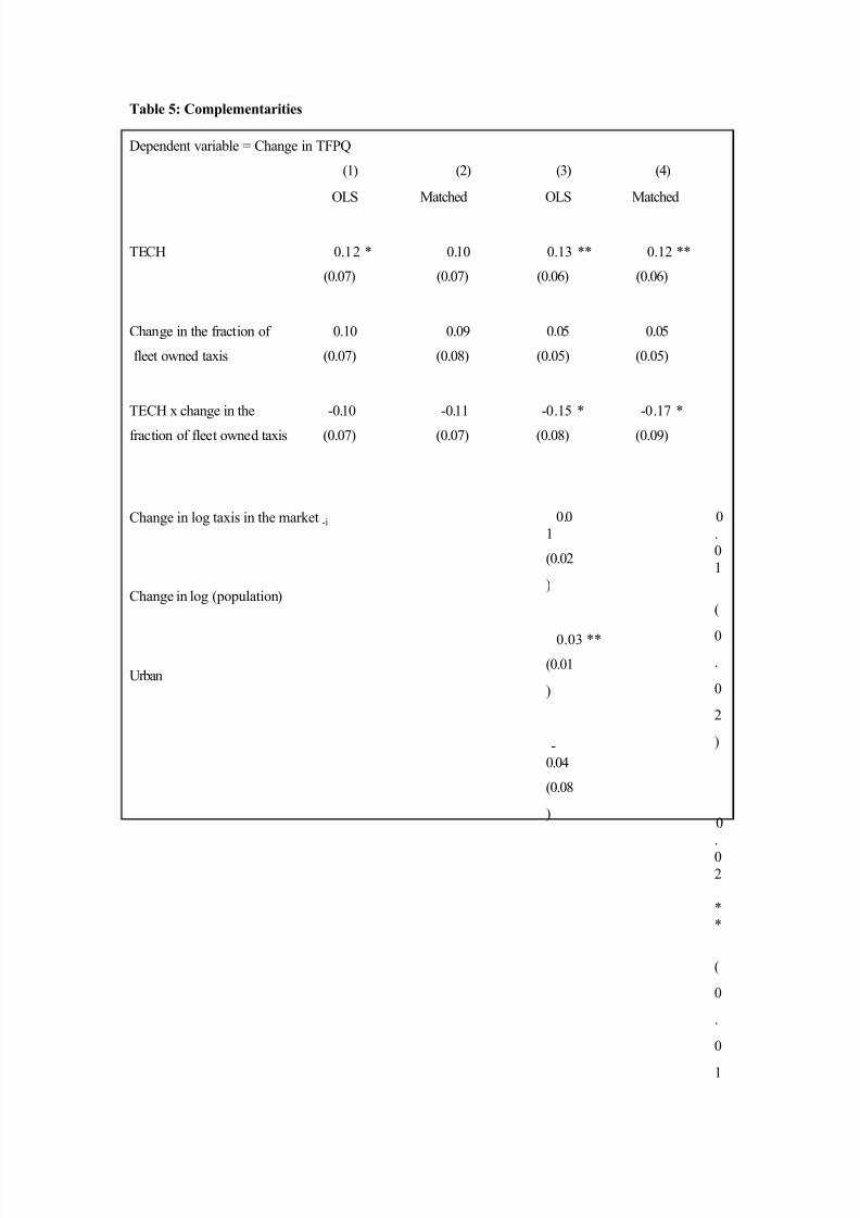
8/8/2019 A_study on Mobile Production
http://slidepdf.com/reader/full/astudy-on-mobile-production 59/66
Table 5: Complementarities
Dependent variable = Change in TFPQ
(1) (2) (3) (4)
OLS Matched OLS Matched
TECH 0.12 * 0.10 0.13 ** 0.12 **
(0.07) (0.07) (0.06) (0.06)
Change in the fraction of 0.10 0.09 0.05 0.05
fleet owned taxis (0.07) (0.08) (0.05) (0.05)
TECH x change in the -0.10 -0.11 -0.15 * -0.17 *
fraction of fleet owned taxis (0.07) (0.07) (0.08) (0.09)
Change in log taxis in the market -i
Change in log (population)
Urban
0.01
(0.02
)
0.03 **
(0.01
)
-0.04
(0.08
)
0.01
(
0.
0
2
)
0.
02 **
(
0
.
0
1
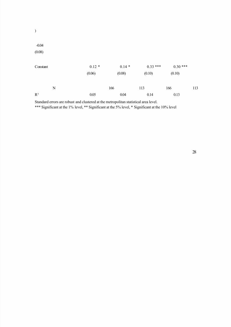
8/8/2019 A_study on Mobile Production
http://slidepdf.com/reader/full/astudy-on-mobile-production 60/66
)
-0.04
(0.08)
Constant 0.12 * 0.14 * 0.33 *** 0.30 ***
(0.06) (0.08) (0.10) (0.10)
N 166 113 166 113
R 2 0.05 0.04 0.14 0.13
Standard errors are robust and clustered at the metropolitan statistical area level.
*** Significant at the 1% level, ** Significant at the 5% level, * Significant at the 10% level
28
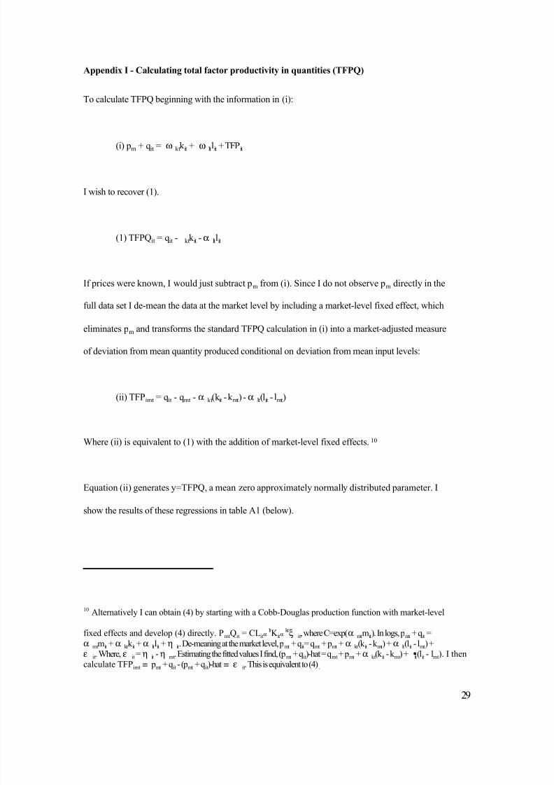
8/8/2019 A_study on Mobile Production
http://slidepdf.com/reader/full/astudy-on-mobile-production 61/66
Appendix I - Calculating total factor productivity in quantities (TFPQ)
To calculate TFPQ beginning with the information in (i):
(i) pm + qit = ω ktk it + ω ltlit + TFPit
I wish to recover (1).
(1) TFPQit = qit - ktk it -α ltlit
If prices were known, I would just subtract pm from (i). Since I do not observe pm directly in the
full data set I de-mean the data at the market level by including a market-level fixed effect, which
eliminates pm and transforms the standard TFPQ calculation in (i) into a market-adjusted measure
of deviation from mean quantity produced conditional on deviation from mean input levels:
(ii) TFPimt = qit - qmt - α kt(k it - k mt) -α lt(lit - lmt)
Where (ii) is equivalent to (1) with the addition of market-level fixed effects.10
Equation (ii) generates y=TFPQ, a mean zero approximately normally distributed parameter. I
show the results of these regressions in table A1 (below).
10 Alternatively I can obtain (4) by starting with a Cobb-Douglas production function with market-level
fixed effects and develop (4) directly. PmtQit = CLitαltK itα
ktξ it, where C=exp(α mtmit). In logs, pmt + qit =α mtmit +α ktk it +α ltlit +η it. De-meaning at the market level, pmt + qit= qmt + pmt +α kt(k it - k mt) +α lt(lit - lmt) +ε it. Where, ε it =η it -η mt. Estimating the fitted values I find, (pmt + qit)-hat = qmt + pmt +α kt(k it - k mt) +lt(lit - lmt). I thencalculate TFPimt ≡ pmt + qit - (pmt + qit)-hat ≡ ε it. This is equivalent to (4).
29

8/8/2019 A_study on Mobile Production
http://slidepdf.com/reader/full/astudy-on-mobile-production 62/66
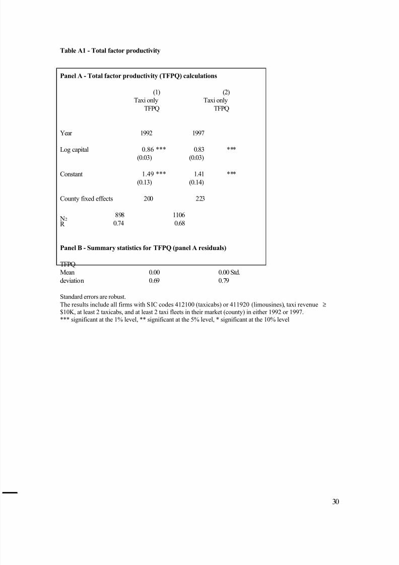
8/8/2019 A_study on Mobile Production
http://slidepdf.com/reader/full/astudy-on-mobile-production 63/66
Table A1 - Total factor productivity
Panel A - Total factor productivity (TFPQ) calculations
(1) (2)
Taxi only Taxi onlyTFPQ TFPQ
Year
Log capital
Constant
County fixed effects
1992
0.86 ***
(0.03)
1.49 ***
(0.13)
200
1997
0.83
(0.03)
1.41
(0.14)
223
***
***
N2R
898
0.74
1106
0.68
Panel B - Summary statistics for TFPQ (panel A residuals)
TFPQ
Mean 0.00 0.00 Std.
deviation 0.69 0.79
Standard errors are robust.The results include all firms with SIC codes 412100 (taxicabs) or 411920 (limousines), taxi revenue ≥$10K, at least 2 taxicabs, and at least 2 taxi fleets in their market (county) in either 1992 or 1997.*** significant at the 1% level, ** significant at the 5% level, * significant at the 10% level
30

8/8/2019 A_study on Mobile Production
http://slidepdf.com/reader/full/astudy-on-mobile-production 64/66

8/8/2019 A_study on Mobile Production
http://slidepdf.com/reader/full/astudy-on-mobile-production 65/66

8/8/2019 A_study on Mobile Production
http://slidepdf.com/reader/full/astudy-on-mobile-production 66/66
Table A3: Adoption of mobile IT networks and productivity
1997 cross-section
Dependent variable = TFPQ
(1) (2) (3) (4)
OLS 2SLS OLS 2SLS
TECH 0.25 *** 0.14 0.20 ** 0.08
(0.09) (0.23) (0.10) (0.28)
Total vehicles 0.00 0.00
(0.00) (0.00)
Log(taxis in the market -i) -0.02 -0.02
(0.03) (0.03)
Log(population) 0.06 0.07
(0.05) (0.05)
Log(square miles) 0.00 0.00
(0.04) (0.04)
Constant -0.58 -0.62
(0.49) (0.48)
N 409 409 409 409
R 2 0.01 n/a 0.02 n/a
Standard errors are robust.
First-state results for regression (2) using lagged (1992) average fleet size in the same market as an
instrument were: IV coefficient 0.005, standard error (0.001). F-stat = 43, Adjusted R 2 = 0.10.
First-state results for regression (4) using lagged (1992) average fleet size in the same market as an
instrument were: IV coefficient 0.004, standard error (0.001). F-stat = 13, Adjusted R 2 = 0.19.
*** Significant at the 1% level, ** Significant at the 5% level, * Significant at the 10% level
32