astrostats 2013 lecture 2 bayesian time series analysis and stochastic...

Astrostats 2013 Lecture 2

Bayesian time series analysis and stochastic processes

C.A.L. Bailer-JonesMax Planck Institute for Astronomy, Heidelberghttp://www.mpia.de/~calj/

Last updated: 2013-06-17 22:20

Contents

1 Key points 2

2 Introduction 3

3 Sinusoidal model and the Bayesian periodogram 3

3.1 An analytic Bayesian periodogram . . . . . . . . . . . . . . . . . . . . . . . . 4

4 Parameter estimation with the sinusoidal model 7

5 A general method for time series modelling 11

5.1 Measurement model . . . . . . . . . . . . . . . . . . . . . . . . . . . . . . . . 12

5.2 Time series model . . . . . . . . . . . . . . . . . . . . . . . . . . . . . . . . . 12

5.3 Likelihood . . . . . . . . . . . . . . . . . . . . . . . . . . . . . . . . . . . . . . 13

6 Stochastic processes 13

6.1 Markov processes . . . . . . . . . . . . . . . . . . . . . . . . . . . . . . . . . . 14

6.2 Describing continuous stochastic processes (Langevin equation) . . . . . . . . 14

6.3 Ornstein–Uhlenbeck process . . . . . . . . . . . . . . . . . . . . . . . . . . . . 15

6.4 Wiener process . . . . . . . . . . . . . . . . . . . . . . . . . . . . . . . . . . . 16

6.5 Historical note . . . . . . . . . . . . . . . . . . . . . . . . . . . . . . . . . . . 17

7 Modelling the OU process 17

8 Parameter estimation with the OU process 18

9 Comparison of sinusoidal and OU process models on real data 22

10 Exercises 24

A Further reading 25

B R functions for the sinusoidal model 26

http://www.mpia.de/~calj/

Astrostats 2013. Lecture 2: Bayesian time series analysis and stochastic processes 2

C R functions for the OU process 28

D Spectral analysis 32

D.1 General concepts . . . . . . . . . . . . . . . . . . . . . . . . . . . . . . . . . . 32

D.2 OU process . . . . . . . . . . . . . . . . . . . . . . . . . . . . . . . . . . . . . 33

1 Key points

• Fitting time series model to data is not fundamentally different from fitting other typesof data: the basic principle remains to define a generative model for the data, a likeli-hood, and a prior over the model parameters. Model comparison can be done as beforeusing the evidence, K-fold cross-validation likelihood, or other methods.

• A fully general solution to fitting an arbitrary model to time series data with arbi-trary noise models on both the signal and time axes is readily obtainable. It can besolved in general through numerical integration, although some common special casesor approximations render simpler solutions.

• Properly defined, the periodogram or power spectrum is closely related to the posteriorprobability density function over the frequency parameter of a sinusoidal model.

• A stochastic time series model is one in which the signal evolution itself has a non-deterministic component, even in the absence of measurement noise. A particularlyuseful model is the Ornstein–Uhlenbeck process, or damped random walk, which hasbeen used to model Brownian motion.

C.A.L. Bailer-Jones


2 Introduction

Bayesian data analysis is a general approach to modelling, and its principles and methodsapply equally well to time series data. In this lecture I will consider just single variable timeseries, in which we are interested in the variation of a single quantity, z, with time, t. Givena set of J events, D = {tj , zj}, we are interested in one or more of the usual three questions:

1. Parameter estimation: Given a model M , which values of its parameters, θ, best de-scribes the data? Or rather, what is the (multidimensional) posterior probability densityfunction (PDF) P (θ|D,M)?

2. Model comparison: Given a set of models {Mi}, which best explains the data? Orrather, what are the values of the model posterior probabilities P (Mi|D)?

3. Prediction: What value do we predict for the time series at some time t′? Or rather,what is P (z|t = t′)?1

3 Sinusoidal model and the Bayesian periodogram

A general model for our data, f(t), we can write as

zj = f(tj) + ε(tj) (1)

where ε(tj) is the noise model. A specific sinusoidal model we could write as

f(t) = A1 cos(ωt) +A2 sin(ωt) (2)

which has three parameters θ = (A1, A2, ω). (This is appropriate only if the data have zeromean, which we can arrange prior to modelling.) A typical noise model is a zero meanGaussian, i.e.

P (zj |θ,M) =1

σj√

2πexp

(− [zj − f(tj)]

2

2σ2j

)(3)

where the {σj} could be parameters of the model which we determine via inference, or theymay be given. Quite often the noise model is taken to be stationary, in which case we canreplace these with a scalar σ, which I will now assume. If we additionally assume the measuredtimes {tj} to be noise-free (“fixed”), then equation 3 is just the likelihood for one data point.Strictly speaking this likelihood should be written P (zj |tj , θ,M), but I make the dependenceon the fixed times implicit, and now write the (noisy) measured data as D = {zj}.

Assuming that the data have been measured independently, then the total likelihood is theproduct of the individual likelihoods

P (D|θ,M) =∏j

1

σj√

2πexp

(− [zj − f(tj)]

2

2σ2

)

=

(1

σ√

2π

)Jexp

(− 1

2σ2

∑j

[zj − f(tj)]2). (4)

1Posed this way, we have averaged over all models. We might be instead interested in P (z|t = t′,M),which has marginalized over the parameters for one model, or even P (z|t = t′, θ,M), for some “optimal” valueof θ.

C.A.L. Bailer-Jones


Inference of the model parameters proceeds in the usual way: we adopt a prior PDF andmultiply this by the likelihood to get the unnormalized posterior. As this does not havean exact closed form in the θ, we may sample it using some Monte Carlo technique, thenuse density estimation to plot the resulting posterior PDF and estimate from this summarystatistics such as the mean, mode and confidence intervals.

If we marginalize the posterior PDF over all parameters other than ω, then we end up withthe one-dimensional (1D) posterior PDF P (ω|D,M), which is the Bayesian periodogram. Bayesian

periodogramThis is already a probability density function, so unlike most other periodograms it does notneed to be calibrated via (often dubious) significance tests.

3.1 An analytic Bayesian periodogram2

A few simple and not very restrictive approximations to the likelihood allow us to extract ananalytic Bayesian periodogram from the above analysis. Expanding the square in equation 4and substituting in equation 2 we can write the likelihood as

P (D|θ,M) ∝ σ−J exp

(− G

2σ2

)(5)

where I have dropped the numerical constant and where

G =∑j

z2j +

∑j

f(tj)2 − 2

∑j

zjf(tj)

=∑j

z2j +

∑j

f(tj)2 − 2[A1R(ω) +A2I(ω)] (6)

with

R(ω) =∑j

zj cos(ωtj) (7)

I(ω) =∑j

zj sin(ωtj) . (8)

Expanding the model term∑j

f(tj)2 = A2

1

∑j

cos2(ωtj) +A22

∑j

sin2(ωtj) + 2A1A2

∑j

cos(ωtj) sin(ωtj) . (9)

When J � 1 this can be simplified using the following approximations∑j

cos2(ωtj) =J

2+

1

2

∑j

cos(2ωtj) ' J

2(10)

∑j

sin2(ωtj) =J

2− 1

2

∑j

cos(2ωtj) ' J

2(11)

∑j

cos(ωtj) sin(ωtj) =1

2

∑j

sin(2ωtj) � J

2. (12)

2This section follows the development in chapter 2 of Bretthorst (1998), with additional derivations andcomments.

C.A.L. Bailer-Jones


In each of these we have the sum of lots of positive and negative terms, and unless we happento have ωtj = n/2 for integer n for all tj , each of these sums is much less than 1, yieldingthe above approximations. This approximation also requires that ωtj � 1, otherwise we willhave cos(2ωtj) ' 1 ∀ i. Thus in addition to requiring a reasonably large amount of data(J � 1), our approximation also requires that we have no low frequency variation in the data(the data have been detrended if necessary).

The consequence of these approximations is that∑j

f(tj)2 ' J

2(A2

1 +A22) (13)

so we can write G in the likelihood (equation 5) as

G ' Jz2 +J

2(A2

1 +A22)− 2[A1R(ω) +A2I(ω)] (14)

where

z2 =1

J

j=J∑j=1

z2j (15)

is the mean square of the data. This form for G will prove useful in the next step.

Often we are interested in the posterior PDF over just the frequency. To find this we mustmultiply the likelihood by the prior PDF and integrate over A1 and A2. For simplicitywe adopt for both amplitudes a uniform prior which stretches from minus infinity to plusinfinity.3 Note that this is an improper prior, i.e. it does not have a finite integral. This isnot a problem here, however, because we are integrating its product with a function whichdrops to zero as the magnitude of the amplitude increases (the likelihood), so the integral– which is just the integral of equation 5 – will converge. From equation 14 can write theintegrand as

exp

(− G

2σ2

)= exp

(−Jz2

2σ2

)exp

(−JA

21

4σ2+R(ω)A1

σ2

)exp

(−JA

22

4σ2+I(ω)A2

σ2

)(16)

We make use of the following standard Gaussian integral for each integration∫ +∞

−∞exp (−ax2 − bx) dx =

√π

aexp

(b2

4a

)(a > 0) . (17)

Thus our integral becomes

∫∫ +∞

−∞exp

(− G

2σ2

)dA1dA2 = exp

(−Jz2

2σ2

)2σ

√π

Jexp

(R(ω)2

Jσ2

)2σ

√π

Jexp

(I(ω)2

Jσ2

)(18)

3We may think of this as being “uninformative” because it is uniform. This description is misleading,however, because a uniform distribution can be made non-uniform by various transformations of the parameter.A distribution uniform over A is not uniform over logA. Is this still “uninformative”?

C.A.L. Bailer-Jones


and so the marginalized posterior of ω and σ (implicitly also adopting uniform priors onthese) is

P (ω, σ|D,M) ∝ σ2−J exp

(−Jz

2

2σ2+R(ω)2 + I(ω)2

Jσ2

). (19)

If σ is given we can absorb the first term in the exponent into the proportionality constantand then have the posterior PDF over ω, the (Bayesian) periodogram Periodogram

forknownnoise

P (ω|D,M) ∝ exp

(W (ω)

σ2

)(20)

where

W (ω) =1

J

[R(ω)2 + I(ω)2

]=

1

J

∣∣∣ j=J∑j=1

zje−iωtj

∣∣∣2 . (21)

is the Schuster periodogram. Arthur Schuster intuitively defined the periodogram as W (ω) Schusterperiodogram1905. We now see a rigorous basis for it in terms of fitting a single component sinusoidal

model to data under some mild assumptions. But the Schuster periodogram itself ignoresthe noise in the data, whereas the Bayesian periodogram (posterior PDF) does not. Notethat the Schuster periodogram is just the magnitude of a discrete Fourier transform of thedata, and it is defined for any sampling of the data: nothing we have done demands uniformsampling.

If σ is instead unknown, then by adopting a prior over σ, multiplying this by the right-hand-side of equation 19 (which is proportional to the likelihood) and then integrating over σ, wewill get the posterior over ω for the case of unknown noise. A convenient prior is the Jeffrey’sprior, P (σ) = 1/σ, which is again an improper prior (and is equivalent to a prior uniform inlog σ). We have

P (ω|D,M) ∝ Q =

∫ ∞0

σ1−J exp

(−Jz

2

2σ2+W (ω)

σ2

)dσ (22)

Writing

a =Jz2

2−W (ω) (23)

and making the substitution x = 1/σ, we can write this as

Q =

∫ ∞0

xJ−3 exp (−ax2) dx . (24)

This is a standard integral, with result

Q =1

2Γ(J − 2

2

)a(2−J)/2 (a > 0, J > 2) . (25)

Absorbing the terms not involving a into the proportionality constant, we can write theposterior PDF over ω as Periodogram

forunknownnoiseP (ω|D,M) ∝

(Jz2

2−W (ω)

)(2−J)/2

. (26)

C.A.L. Bailer-Jones


The condition a > 0 implies Jz2

2 > W (ω). As the maximum value of W (ω) is z2, thiscondition is always met provided J > 2, a condition we already required earlier. The factthat a > 0 also ensures that the right-hand-side of equation 26 is always defined and ispositive, a requirement for a probability density function.

In summary, we have derived analytic forms for the Bayesian periodogram for the case ofconstant noise standard deviation, where this is known (equation 20) and unknown (equa-tion 26). These are valid for any time sampling. In both cases we have assumed that wehave a reasonably large amount of data, and that the data are zero mean and lacking anylow frequency trend. We will use them in the next section.

Bretthorst (1998) goes on to show (in his chapter 3) how the above can be extended to amodel with multiple sinusoidal components, or indeed any other set of basis functions. Heshows that the simplification to “analytic” forms for the PDF – similar to those derivedabove – can be achieved through a diagonalization of these basis functions (i.e. forming anew orthogonal basis set through linear combinations of the original set). This accommodateswhatever time sampling we have in the data.

4 Parameter estimation with the sinusoidal model

The following R code shows how we can implement the ideas in the previous sections. Itmakes use of the functions defined in the appendix in section B. Plots generated by this codeare shown in Figures 1 to 4.

The parameters are A1, A2, and ν, where ω = 2πν. There are called theta in the code.

Concerning the priors, I adopt Gaussian distributions for the two amplitude parameters,with zero mean, and standard deviations on the scale of the amplitude of the data. As thefrequency must be positive, I use a gamma distribution for its prior. The gamma distributionis characterized by two parameters, shape and scale. I adopt a shape parameter greater than1 to ensure that very low frequencies are suppressed (I use 1.5), and a scale parameter whichyields non-vanishing probabilities for the highest frequencies I expect. In real problems,we are likely to have some idea of this from the nature of the phenomenon, or from whatthe measurements may have been sensitive to. Thus in this implementation there are three“hyperparameters” (parameters of the prior PDF), the Gaussian standard deviation for eachof A1 and A2 and the gamma scale for frequency. There are called alpha in the code.

R file: Rcode/exp_sinusoidal.R

# C.A.L. Bailer-Jones

# Astrostats 2013

# This file: exp_sinusoidal.R

# R code for experimenting with the sinusoidal model

source("sinusoidal.R")

source("monte_carlo.R") # provides metrop() and make.covariance.matrix()

set.seed(200)

# Generate a time series from a sinusoidal model

C.A.L. Bailer-Jones


0 5 10 15 20

−2

−1

01

2

time

sign

al

measured = black, model = red

0 5 10 15 20

−2

−1

01

2

time

sign

al

measured = black, model = red

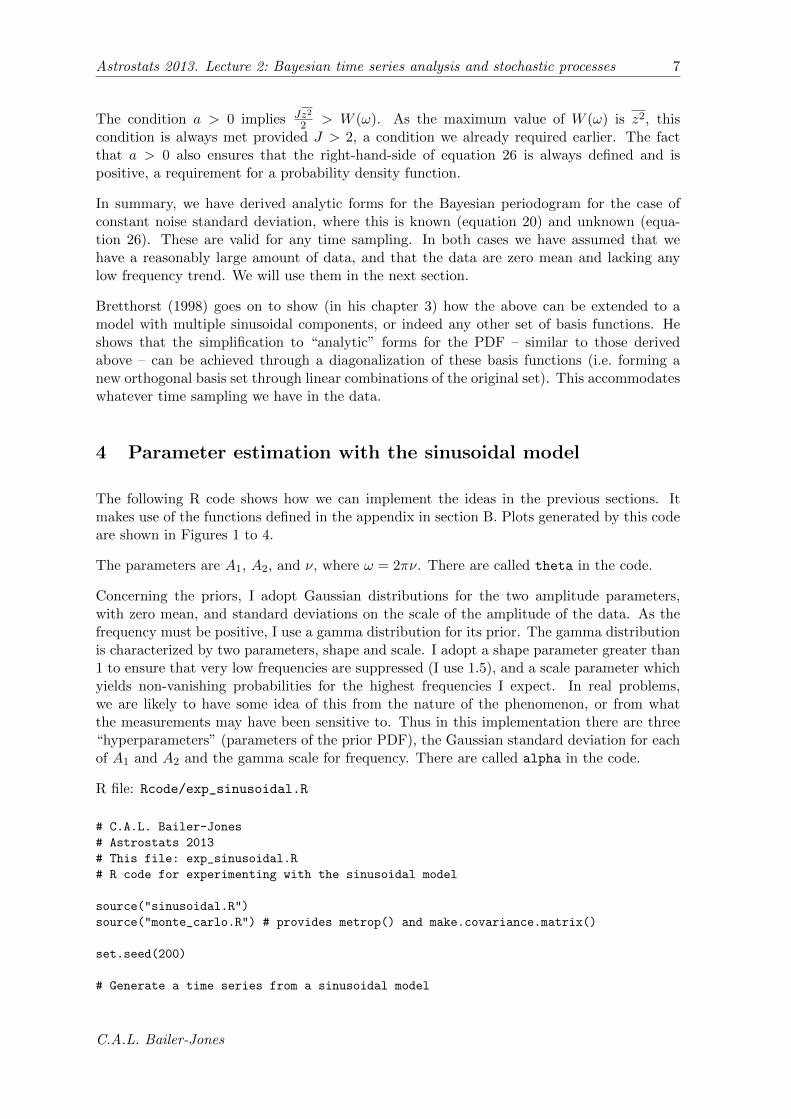
Figure 1: Data set (black) generated from the sinusoidal model (red), equation 2. The trueparameters are A1 = 1, A2 = 1, ω = 2π ∗ 0.5. The same data are shown in both panels.

02

46

8

sampFreq

pow

er (

norm

aliz

ed)

Schuster periodogram

020

60

sampFreq

log1

0pos

t

assuming common sigma

0.2 0.4 0.6 0.8 1.0

−10

−5

05

sampFreq

log1

0pos

t

assuming unknown sigma

frequency

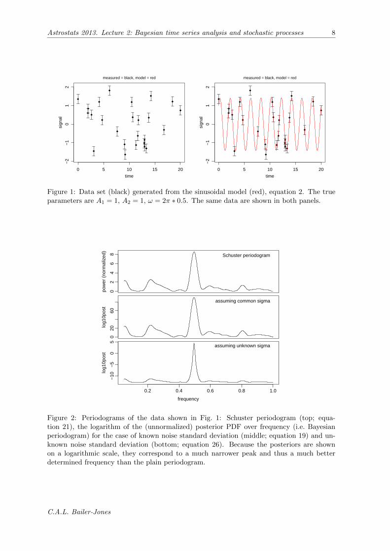
Figure 2: Periodograms of the data shown in Fig. 1: Schuster periodogram (top; equa-tion 21), the logarithm of the (unnormalized) posterior PDF over frequency (i.e. Bayesianperiodogram) for the case of known noise standard deviation (middle; equation 19) and un-known noise standard deviation (bottom; equation 26). Because the posteriors are shownon a logarithmic scale, they correspond to a much narrower peak and thus a much betterdetermined frequency than the plain periodogram.

C.A.L. Bailer-Jones


0 5000 15000 25000

0.4

0.8

1.2

iteration

a1

0.2 0.4 0.6 0.8 1.0 1.2 1.4

0.0

1.0

2.0

a1

dens

ity

0 5000 15000 25000

0.0

1.0

2.0

iteration

a2

0.0 0.5 1.0 1.5 2.0

0.0

0.6

1.2

a2

dens

ity

0 5000 15000 25000

0.25

0.40

iteration

freq

0.20 0.30 0.40 0.50

040

80

freq

dens

ity

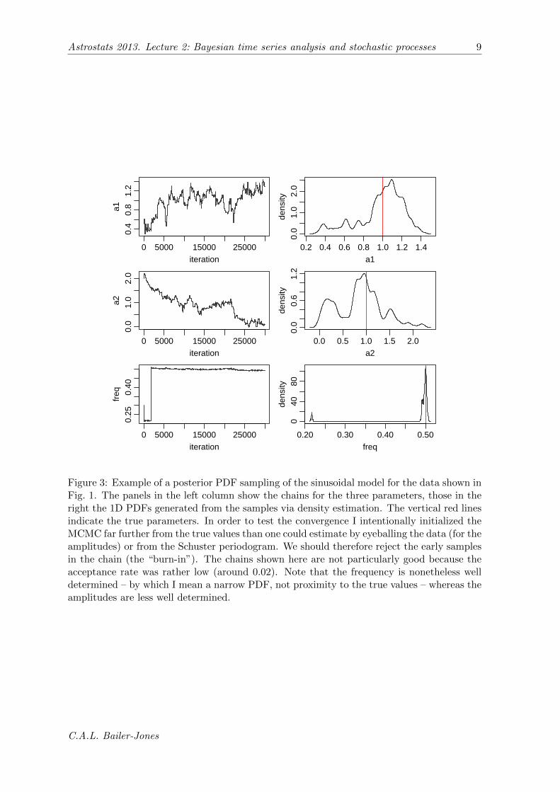
Figure 3: Example of a posterior PDF sampling of the sinusoidal model for the data shown inFig. 1. The panels in the left column show the chains for the three parameters, those in theright the 1D PDFs generated from the samples via density estimation. The vertical red linesindicate the true parameters. In order to test the convergence I intentionally initialized theMCMC far further from the true values than one could estimate by eyeballing the data (for theamplitudes) or from the Schuster periodogram. We should therefore reject the early samplesin the chain (the “burn-in”). The chains shown here are not particularly good because theacceptance rate was rather low (around 0.02). Note that the frequency is nonetheless welldetermined – by which I mean a narrow PDF, not proximity to the true values – whereas theamplitudes are less well determined.

C.A.L. Bailer-Jones


●

●

●

●

●

●

●

●

●

●

●

●

●

●

●

●

●

●

●

●

●

●

●

●

●

0 5 10 15 20

−2

−1

01

2

time

sign

al

●

●

●

●

●

●

●

●

●

●

●

●

●

●

●

●

●

●

●

●

●

●

●

●

●

Figure 4: Predicted data at the mode (in blue) and mean (in green) of the posterior PDF inFigure 3. Overplotted are the data (black points) and true model (in red).

sinmod <- list(a1=1, a2=1, freq=0.5)

eventTimes <- sort(c(0, 20, runif(n=23, min=0, max=20)))

ysigma <- 0.25

obsdata <- gen.sinusoidal(sinmod=sinmod, eventTimes=eventTimes, ysigma=ysigma)

# Plot data and overplot with true sinusoidal model

oplot.obsdata.sinusoidal(obsdata=obsdata, sinmod=sinmod, ploterr=TRUE, fname="sindat1.pdf")

oplot.obsdata.sinusoidal(obsdata=obsdata, sinmod=NULL, ploterr=TRUE, fname="sindat2.pdf")

# Model assumes data are zero mean

obsdata[,3] <- obsdata[,3] - mean(obsdata[,3])

# Calculate and plot Schuster periodogram and derived posterior PDFs over frequency

schuster(obsdata=obsdata, minFreq=0.05, maxFreq=1, NFreq=1e3, fname="schuster.pdf")

# For the following inference we sample over the three parameters

# theta = c(a1, a2, freq). The hyperparameters of the prior PDFs are

# alpha = c(sd_a1, sd_a2, scale_freq), with mean_a1, mean_a2, and

# shape_freq fixed in the definitions of the functions.

alpha <- c(1, 1, 1) # c(sd_a1, sd_a2, scale_freq)

# Use MCMC to sample posterior for sinusoidal model: c(a1, a2, freq)

sampleCov <- make.covariance.matrix(sampleSD=c(0.05, 0.05, 0.1), sampleCor=0)

thetaInit <- c(0.5, 2, 0.3)

postSamp <- metrop(func=logpost.sinusoidal, thetaInit=thetaInit, Nburnin=0,

Nsamp=3e4, verbose=1e3, sampleCov=sampleCov,

obsdata=obsdata, alpha=alpha)

# Plot MCMC chains and use density estimation to plot 1D posterior PDFs from these.

thetaTrue <- as.numeric(sinmod)

parnames <- c("a1", "a2", "freq")

pdf("sindat_mcmc.pdf", width=7, height=6)

par(mfrow=c(3,2), mar=c(3.0,3.0,0.5,0.5), oma=c(1,1,1,1), mgp=c(1.8,0.6,0), cex=1.0)

for(p in 3:5) { # columns of postSamp

plot(1:nrow(postSamp), postSamp[,p], type="l", xlab="iteration", ylab=parnames[p-2])

C.A.L. Bailer-Jones


postDen <- density(postSamp[,p], n=2^10)

plot(postDen$x, postDen$y, type="l", xlab=parnames[p-2], ylab="density")

abline(v=thetaTrue[p-2], col="red")

}

dev.off()

# Find MAP solution and mean solutions and overplot on data

posMAP <- which.max(postSamp[,1]+postSamp[,2])

(thetaMAP <- postSamp[posMAP, 3:5])

(thetaMean <- apply(postSamp[,3:5], 2, mean)) # Monte Carlo integration

locplot <- function(theta, col) {

tsamp <- seq(from=min(eventTimes), to=max(eventTimes), length.out=1e3)

omegat <- 2*pi*theta[3]*tsamp

modpred <- theta[1]*cos(omegat) + theta[2]*sin(omegat)

lines(tsamp, modpred, col=col, lw=1)

}

pdf("sindat_fits.pdf", width=6, height=5)

par(mfrow=c(1,1), mgp=c(2.0,0.8,0), mar=c(3.5,4.0,1.0,1.0), oma=c(0,0,0,0), cex=1.2)

plotCI(obsdata[,1], obsdata[,3], xlab="time", ylab="signal", uiw=obsdata[,4], gap=0)

locplot(theta=as.numeric(sinmod), col="red")

locplot(theta=thetaMAP, col="blue")

locplot(theta=thetaMean, col="green")

dev.off()

5 A general method for time series modelling4

In section 3 I made two implicit assumptions. First, I assumed that the process itself wasdeterministic. Randomness arose only on account of measurement noise. Yet some processesare intrinsically random (or stochastic), even if there is no measurement noise. These arediscussed further in section 6. Second, I assumed that the times at which the data wereobtained were subject to no uncertainty. This is not true in general, and often not in practice,e.g. astronomical ages derived from photometric redshifts or stellar clusters, or geological agesfrom the fossil record.

For this more general case we first need a more general notation. Let t and z now correspondto the true time and signal (respectively), not to the measured values. Instead, for each eventj, our measurement of its time of the event, tj , is sj with a standard deviation (estimatedmeasurement uncertainty) σsj , and our measurement of the signal of the event, zj , is yj witha standard deviation (estimated measurement uncertainty) σyj .

For shorthand I write Dj = (sj , yj), the (noisy) data for one event, and σj = (σsj , σyj ). Themeasurement model (or noise model) describes the probability of observing the measuredvalues for a single event given the true values and the estimated uncertainties: it givesP (Dj |tj , zj , σj). The σj are considered fixed parameters of the measurement model.

M is a stochastic time series model with parameters θ. It specifies P (tj , zj |θ,M), the prob-ability of observing an event at time tj with signal zj .

To do inference we need to derive the likelihood, P (D|σ, θ,M), where D = {Dj} and σ =

4This section is an introduction to the method explained in detail in Bailer-Jones (2012).

C.A.L. Bailer-Jones


{σj}. (We can also write this as P (D|θ,M) because σ is fixed.) We will see below how toderive it in terms of the measurement model and time series model, but let’s first examinethese a little more.

5.1 Measurement model

If t and z have no bounds and the measurement uncertainties are standard deviations, then anappropriate choice for the measurement model is a two-dimensional Gaussian in the variables(sj , yj) for event j. If we assume no covariance between the variables then this reduces tothe product of two 1D Gaussians

P (Dj |tj , zj , σj) =1√

2πσsje−(sj−tj)2/2σ2

sj1√

2πσyje−(yj−zj)2/2σ2

yj . (27)

(The two terms are normalized with respect to sj and yj respectively.) If we had otherinformation about the measurement, e.g. asymmetric error bars, strictly positive signals, oruncertainties which are not standard deviations, then we should adopt a more appropriatedistribution.

5.2 Time series model

We can write the time series model as the product of two components

P (tj , zj |θ,M) = P (zj |tj , θ,M)P (tj |θ,M) (28)

which I will refer to as the signal and time components respectively.

The process may be subject to a stochastic component (which has nothing to do with mea-surement noise). In that case it is useful to express the signal component itself using twoindependent subcomponents: (1) the stochastic model of the variation in the signal, z; (2) adeterministic function which defines the time-dependence of its mean.

The stochastic subcomponent might be a Gaussian

P (zj |tj , θ,M) =1√2πλ

e−(zj−η[tj ])2/2λ2

(29)

where θ = (η, λ) are the “parameters” of the distribution: η[tj ] is the expected true signalat true time tj ; λ

2 is a parameter which reflects the degree of stochasticity (in this case thevariance) of the process.

For a sinusoidal process, the deterministic subcomponent can be written as before

η = A1 cos(ωt) +A2 sin(ωt) (30)

which has parameters (A1, A2, ω).

The final term in equation 28, P (tj |θ,M), reflects the stochasticity in the event times them-selves. This is used to model the probability distribution over the times of events which areconsidered non-deterministic in the problem context, such as supernovae or asteroid impacts.If there is no stochasticity in the event times, then a uniform distribution should be adopted.

C.A.L. Bailer-Jones


5.3 Likelihood

The probability of observing data Dj from time series model M with parameters θ when theuncertainties are σj , is P (Dj |σj , θ,M), the event likelihood. This is obtained by marginalizingover the true, unknown event time and signal

P (Dj |σj , θ,M) =

∫∫tj ,zj

P (Dj , tj , zj |σj , θ,M) dtjdzj

=

∫∫tj ,zj

P (Dj |tj , zj , σj , θ,M)P (tj , zj |σj , θ,M) dtjdzj

=

∫∫tj ,zj

P (Dj |tj , zj , σj)︸︷︷︸Measurement model

P (tj , zj |θ,M)︸︷︷︸Time series model

dtjdzj (31)

where the time series model and its parameters drop out of the first term because Dj isindependent of this once conditioned on the true variables, and the measurement model (viaσj) drops out of the the second term because it has nothing to do with the predictions of thetime series model. For specific, but common, situations, this two-dimensional integral can beapproximated by a 1D integral or even a function evaluation.

If we have a set of J events for which the ages and signals have been estimated independentlyof one another, then the probability of observing all these, the likelihood, is

P (D|σ, θ,M) =∏j

P (Dj |σj , θ,M) . (32)

Armed with the likelihood for our given measurement model, time series model, and measureddata, and adopting suitable priors over the model parameters, we can now calculate all theusual things we need for Bayesian inference (posterior PDFs, evidences etc.), typically usingMCMC methods to sample the likelihood. Specific models and an application to brown dwarflight curves can be found in Bailer-Jones (2012). This also makes use of stochastic models,which we now turn to.

6 Stochastic processes

A stochastic process is one in which some aspect of the system evolves randomly. Normallywe do not take this definition to include the effects of measurement noise, as then almostall observed processes would appear stochastic. Rather, we take stochastic to mean that theevolution of the system itself has a non-deterministic component.

If {zj} is the state of a stochastic system at times {tj}, then the multidimensional PDFP ({zj}, {tj}) completely describes the system. The conditional PDF of future events (j > 0)in terms of past events can then be written

P (zj+1, tj+1; zj+2, tj+2; . . . |z0, t0; zj−1, tj−1; . . .) =P ({zj}, {tj})

P (z0, t0; zj−1, tj−1, . . .)(33)

where for convenience I’ve adopted the notation such that . . . ≥ tj+1 ≥ tj ≥ tj−1 ≥ . . .. Asimple stochastic system is one in which all events are independent,

P ({zj}, {tj}) =∏j

P (zj , tj) (34)

C.A.L. Bailer-Jones


an example of which is a pure noise process.

In this section I will use the notation N (x;µ, V ) to indicate a random number drawn from aGaussian PDF with mean µ and variance V . The x indicates that a different random numberis drawn for every x, i.e. N (x;µ, V ) is statistically independent of N (x′;µ, V ) if x 6= x′. N (x)is a shorthand for N (x;µ = 0, V = 1).

6.1 Markov processes

A Markov process is a specific type of stochastic process in which the future value of thestate variable is independent of the past values conditioned on the present value, i.e.

P (zj+1, tj+1; zj+2, tj+2; . . . |z0, t0; zj−1, tj−1; . . .) = P (zj+1, tj+1; zj+2, tj+2; . . . |z0, t0) . (35)

Such “one step memory” processes are useful in practice, because a chain of past dependenciescan then be written as a probability conditional on only one previous time step, e.g.

P (z1, t1; z2, t2|z0, t0) = P (z2, t2|z1, t1)P (z1, t1|z0, t0) (36)

Markov processes are widely applicable, because many stochastic processes can be reducedto a Markov process. For example, if we had a “two step memory” process, we could convertit into two Markov processes.

6.2 Describing continuous stochastic processes (Langevin equation)

A general first order differential equation which describes the evolution of a continuous statevariable z(t) is

dz

dt= A(z, t) . (37)

If A is a deterministic function then z is a deterministic process. If we want the differentialequation to describe a stochastic process, then we may add to the right-hand-side of thisa stochastic term. The differential equation is then referred to as a Langevin equation. Itturns out that in order to keep this equation self-consistent, we are limited in what kind ofstochastic term we can add. If z(t) is to describe a continuous Markov process, then thefollowing three conditions must apply, with dz = z(t+ dt)− z(t),

1. dz depends only on z, t and dt (this makes it Markov),

2. dz depends smoothly on z, t and dt,

3. z is continuous in the sense that dz → 0 as dt→ 0 for all t and z.

It turns out that the general form of the Langevin equation which satisfies this is

dz = A(z, t)dt+N (t)√D(z, t)dt (38)

where A and D are any smooth functions and D is non-negative. A and D are sometimescalled the drift and diffusion terms respectively. The presence of the second term on theright-hand-side makes this equation a stochastic differential equation. The square-root of dtmay be unfamiliar. We could write the second term instead as N (t; 0, dt)

√D(z, t), in which

N (t; 0, dt) is a Gaussian random variable with variance dt.

C.A.L. Bailer-Jones


6.3 Ornstein–Uhlenbeck process

The Ornstein–Uhlenbeck (OU) process is a particular but widely-used description of a stochas-tic process. It has a Langevin equation with constant drift and diffusion terms

dz = −1

τzdt+ c1/2N (t; 0, dt) (t > 0) (39)

where τ and c are positive constants, the relaxation time (dimension t) and the diffusion con-stant (dimension z2t−1) respectively. The OU process can also be seen as the continuous-timeanalogue of the discrete-time AR(1) (autoregressive) process, and so is sometimes referred toas the (or a) CAR(1) process. It turns out that in the context of Brownian motion, z(t) is agood description of the velocity of the particle.

The OU process is stationary, Gaussian and Markov.5 The solution of equation 39 is thePDF of z(t) given z0 = z(t= t0) for any t > t0

P (z|t, z0, t0) = N (z;µz, Vz) where

µz = z0υ

Vz =cτ

2(1− υ2)

υ = e−(t−t0)/τ . (40)

The relaxation time determines the time scale over which the mean and variance change. Thediffusion constant determines the amplitude of the variance. The OU process z(t) is a mean-reverting process: for t − t0 � τ the mean tends towards zero and the variance asymptotesto cτ/2 (for finite τ).

It follows from equation 40 that z(t) is the sum of z0υ and a random number drawn from azero-mean Gaussian with time-dependent variance. Thus given the event zj−1(tj−1), we canwrite down an update equation (or generative model) for the state at the next time step,zj(tj), as update

equationfor OUprocess

zj = zj−1υ + N (z)√Vz (41)

where now

υ = e−(tj−tj−1)/τ (42a)

Vz =cτ

2(1− υ2) . (42b)

For a given sequence of time steps, (t0, t1, . . .), we can use this to simulate an OU process.Because the time series is stochastic and must be calculated at discrete steps, then even fora fixed random number seed, the generated time series depends on the actual sequence ofsteps. Some examples are shown in Fig. 5.

We can then show that zj has a Gaussian distribution with mean and variance

µ[zj ] = µ[zj−1]υ (43a)

V [zj ] = V [zj−1]υ2 + Vz (43b)

5It is actually the only stochastic process which has these three properties.

C.A.L. Bailer-Jones


−15

−5

05

10−

15−

50

510

0 20 60 100

−15

−5

05

10

0 20 60 100 0 20 60 100 0 20 60 100time

sign

al

Figure 5: Examples of time series generated from the OU process using the update equation(equation 41). The columns from left to right have τ = (1, 10, 100, 1000) respectively. Therows differ only in the random number sequence used in the update equation. The otherparameters are fixed in all cases to c = 1, µ[z1] = 0, V [z1] = 0. All time series are calculatedwith the same uniform time step (0.1) and all panels have the same scales. Plot generatedby R code Rcode/plot OUprocess.R.

respectively. This is subtly different from the update equation, because it concerns theexpected distribution of zj in terms of the expected distribution at the previous time step.It has an additional variance term beyond Vz, because the uncertainty (variance) in zj isincreased by the uncertainty in zj−1.

6.4 Wiener process

The Wiener process can be considered as a special case of the OU process in which therelaxation time scale is infinite, τ →∞ in equation 39, i.e. there is no damping. EquivalentlyA = 0 in equation 38. With υ = e−∆t/τ , υ → 1 and6 τ(1 − υ2) → (∆t)2. The PDF of z(t)

6Using a Taylor expansion

τ(1− e−2(∆t)/τ ) = τ

[1−

(1− 2∆t

τ+

1

2!

(2∆t

τ

)2

− . . .

)]

= τ

[2∆t

τ− 1

2!

(2∆t

τ

)2

+ . . .

]= 2∆t as τ →∞ .

C.A.L. Bailer-Jones


remains Gaussian as in equation 40, but the mean and variance become (with ∆t = t− t0)

µz = z0

Vz = c(t− t0) . (44)

There is no damping, so the variance of the state variable grows monotonically with time, andthis is not a stationary process. Yet as the expectation value of the state variable is constant,this Wiener process is referred to as being driftless. The Wiener process is sometimes takento describe (in a somewhat idealized form) the position of a particle undergoing Brownianmotion.

6.5 Historical note

The Langevin equation and the Wiener and OU processes all evolved from various approachesto modelling Brownian motion. Einstein modelled Brownian motion with a kinematic ap-proach, solving a partial differential equation of the PDF of the particle position (what wetoday would call a special case of the Fokker-Planck equation). Langevin instead adopted adynamic approach, applying Newton’s second law to a typical particle, and writing

dz

dt= βz + η(t) . (45)

where z is the velocity of the particle, with constant β and where the stochastic force, η(t), issubject to 〈η(t)〉 = 0 and 〈η(t)η(t′)〉 = c δ(t− t′) for some constant c. Einstein and Langevinessentially arrived at the same result by different methods, but both approaches had issuesconcerning the assumption and approximations. Ornstein and Uhlenbeck generalized andimproved upon them.

7 Modelling the OU process

This is a little technical. An qualitative summary is given in section 8

Given a set of data D = {Dj} with measurement uncertainties σ = {σj}, we can in principlecalculate the likelihood and thus posterior PDF over the model parameters of a stochasticprocess. This is, however, not quite so straight forward even for a Markov process, becausethe time series model, P (zj , tj |θ,M), which appears in the equation for the likelihood (equa-tion 32), now depends on the PDF at the previous time step. A relatively simple solutioncan nonetheless be obtained if we can assume uncertainties on the times to be negligible,and if both the signal measurement model and the stochastic part of the time series modelare Gaussian. The latter is the case for the OU process. The result is a recurrence relationin which each event likelihood is a Gaussian distribution with mean and variance dependingon both the signal uncertainties for the present and previous events and the variance of theOU process (which depends on the time step size). A full explanation and derivation can befound in section A.2 of Bailer-Jones (2012). Below I just give the result, which we will thenuse to analyse some data.

C.A.L. Bailer-Jones


Starting from equation 31, making the above assumptions, and using the properties of theOU process, we find that we can write the event likelihood as a Gaussian

P (Dj |σj , θ,M) =1

T2 − T1

∫zj

P (yj |zj , σyj )P (zj |tj , θ,M) dzj

=1

T2 − T1

1√2πV [yj ]

exp

(−(yj − µ[yj ])

2

2V [yj ]

)(T1 < tj < T2) (46)

which has mean and variance

µ[yj ] = 0 + µ[zj ] (47a)

V [yj ] = σ2yj + V [zj ] (47b)

respectively, with µ[zj ] and V [zj ] given by equation 43. For simplicity I have additionallyassumed that the time component of the time series model, P (tj |θ,M), is uniform from T1

to T2.

As this is a Markov process, the likelihood depends on the previous time step through µ[zj−1]and V [zj−1] appearing in equation 43. These we must estimate using the data at that previoustime step. How, for any time step j (such as j − 1), do the values of µ[zj ] and V [zj ] dependon yj and σyj? This is equivalent to asking what is the posterior PDF over zj using boththe data at tj and the prior value of zj (which is the posterior from the previous time step).This is given by Bayes theorem. It turns out that this posterior PDF over zj is a Gaussianwith mean and variance

µ′[zj ] =yjV [zj ] + µ[zj ]σ

2yj

V [zj ] + σ2yj

(48a)

V ′[zj ] =V [zj ]σ

2yj

V [zj ] + σ2yj

(48b)

respectively, where the prime symbol is used to distinguish these posterior moments fromthe prior ones in equation 43. It is these quantities which we then use at the next event asthe estimates of the mean and variance of z. Thus, at iteration (event) j, when we evaluateequation 47 )and hence the likelihood), we use µ′[zj−1] and V ′[zj−1] as our estimates ofµ[zj−1] and V [zj−1]. This is how we introduce a dependence on the previous measurement(the Markov property). We then calculate the mean and variance of the posterior for zj usingequation 48, and will then use these in the next iteration. The result is a recurrence relationfor the posterior PDF of zj . At each time step we can siphon off the relevant quantities inorder to calculate the event likelihood (equation 46).

To initialize the process we must specify initial values µ[z1] and V [z1]. We use these inequation 47 to calculate µ[y1] and V [y1] and hence the likelihood for the first event, y1, fromequation 46. We then calculate the posterior moments using equation 48. For the next event,j = 2, these posterior moments are assigned to µ[zj−1] and V [zj−1] in equation 43 and thelikelihood calculated. The procedure is iterated through all the events.

8 Parameter estimation with the OU process

The following R code estimates the posterior PDF for an OU process using the ideas in theprevious section. It makes use of the functions defined in the appendix in section C.

C.A.L. Bailer-Jones


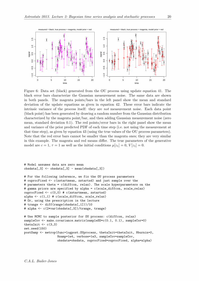
I first simulate an OU process at a series of time steps using the update equation (equa-tion 41). The mean and standard deviation of the state variable are shown as the magentapoints/error bars in the left panel of Figure 6. This is the true process: there is no mea-surement noise. From each of these a value is drawn and measurement noise added: this isshown as the black point/error bar. These, together with value for the OU process parame-ters, are then used to predict the process. The mean and variance of the predicted PDF ateach time step is shown with the red points/error bars in the right panel of Figure 6. As aMarkov process, each of these predictions uses the data at just the previous data point. This“prior” prediction of event j is then combined with the data at event j to make a “posterior”prediction (equation 48; not plotted), which is propagated by equation 43 to give the priorprediction for the next event.

The R code uses MCMC to sample the posterior PDF over the OU process parameters. Ateach parameter sample, the whole OU process is predicted and the likelihood calculated asdescribed in section 7. An example of the sampling is show in Figure 7.

The OU process as defined has four parameters, c, τ , µ[z1], and V [z1]. The latter two are takenas fixed in the following. In practice we may choose to set µ[z1] to the initial value of the timeseries, and V [z1] = 0, which I do here. Concerning the priors, I use the gamma distributionsfor both c and τ , which forces their values to be positive. To suppress vanishingly smallvalues, I set the shape parameter of the gamma distribution to be 1.5. The scale parametersI set as follows. For τ , I set it to tenth of the duration of the time series. This is somewhatarbitrary, so sensitivity to it should be checked. As the long-term variance of an OU processis cτ/2, then I set the scale for c to be this asymptotic value, 2ς2/τ , where ς is the standarddeviation of the time series. Thus there are two “hyperparameters” (parameters of the priorPDF), called alpha in the code.

R file: Rcode/exp_OUprocess.R


# Astrostats 2013

# This file: exp_OUprocess.R

# R code for experimenting with modelling the OU process

source("OUprocess.R")

source("monte_carlo.R")

set.seed(102)

# Generate a time series from an OU process

ouproc <- list(diffcon=1, relax=1, zstartmean=0, zstartsd=0)

eventTimes <- sort(c(0, 20, runif(n=48, min=0, max=20)))

ysigma <- 0.1

temp <- gen.OUprocess(ouproc=ouproc, eventTimes=eventTimes, ysigma=ysigma)

obsdata <- temp$obsdata

procDist <- temp$procDist

# Plot data, ... first overplotting the distributions for each point from the true process

# i.e. the mean and sd of the update equation

oplot.obsdata.OUprocess(obsdata=obsdata, procDist=procDist, fname="ouprocdat1.pdf")

# ... then overplotting the prior PDF evaluated for the OU process at the given parameters

oplot.obsdata.OUprocess(obsdata=obsdata, ouproc=ouproc, fname="ouprocdat2.pdf")

C.A.L. Bailer-Jones


0 5 10 15 20

−1.

0−

0.5

0.0

0.5

1.0

1.5

time

sign

almeasured = black, true process = magenta, model prior = red

0 5 10 15 20

−1.

0−

0.5

0.0

0.5

1.0

1.5

time

sign

al

measured = black, true process = magenta, model prior = red

Figure 6: Data set (black) generated from the OU process using update equation 41. Theblack error bars characterize the Gaussian measurement noise. The same data are shownin both panels. The magenta points/bars in the left panel show the mean and standarddeviation of the update equations as given in equation 42. These error bars indicate theintrinsic variance of the process itself: they are not measurement noise. Each data point(black point) has been generated by drawing a random number from the Gaussian distributioncharacterized by the magenta point/bar, and then adding Gaussian measurement noise (zeromean, standard deviation 0.1). The red points/error bars in the right panel show the meanand variance of the prior predicted PDF of each time step (i.e. not using the measurement atthat time step), as given by equation 43 (using the true values of the OU process parameters).Note that the red error bars cannot be smaller than the magenta ones; they are very similarin this example. The magenta and red means differ. The true parameters of the generativemodel are c = 1, τ = 1 as well as the initial conditions µ[z1] = 0, V [z1] = 0.

# Model assumes data are zero mean


# For the following inference, we fix the OU process parameters

# ouprocFixed <- c(zstartmean, zstartsd) and just sample over the

# parameters theta = c(diffcon, relax). The scale hyperparameters on the

# gamma priors are specified by alpha = c(scale_diffcon, scale_relax)

ouprocFixed <- c(0,0) # c(zstartmean, zstartsd)

alpha <- c(1,1) # c(scale_diffcon, scale_relax)

# Or, using the prescription in the lecture

# trange <- diff(range(obsdata[,1]))/10

# alpha <- c(2*var(obsdata[,3])/trange, trange)

# Use MCMC to sample posterior for OU process: c(diffcon, relax)

sampleCov <- make.covariance.matrix(sampleSD=c(0.1, 0.1), sampleCor=0)

thetaInit <- c(3,3)

set.seed(150)

postSamp <- metrop(func=logpost.OUprocess, thetaInit=thetaInit, Nburnin=0,


obsdata=obsdata, ouprocFixed=ouprocFixed, alpha=alpha)

C.A.L. Bailer-Jones


0 2000 6000 10000

0.5

1.0

1.5

2.0

2.5

iteration

diffc

on

0.5 1.0 1.5 2.0 2.5 3.0

0.0

0.4

0.8

1.2

diffcon

dens

ity

0 2000 6000 10000

0.5

1.5

2.5

3.5

iteration

rela

x

0 1 2 3

0.0

0.4

0.8

1.2

relax

dens

ity

Figure 7: Example of a posterior PDF sampling of the OU process model for the data shownin Fig. 6. The panels in the left column show the chains for the two parameters c (“diffcon”)and τ (“relax”). The panels on the right show the 1D PDFs generated from the samples viadensity estimation. The vertical red lines indicate the true parameters.

# Plot MCMC chains and use density estimation to plot 1D posterior PDFs from these.

thetaTrue <- as.numeric(ouproc[1:2])

parnames <- c("diffcon", "relax")

pdf("ouprocdat_mcmc.pdf", width=7, height=6)






abline(v=thetaTrue[p-2], col="red")

}

dev.off()

C.A.L. Bailer-Jones


51000 51500 52000 52500 53000 53500 54000 54500

−0.

20.

20.

6

days

mag

51000 51500 52000 52500 53000 53500 54000 54500

−0.

150.

000.

15

days

mag

51000 51500 52000 52500 53000 53500 54000 54500

−0.

20.

00.

2

days

mag

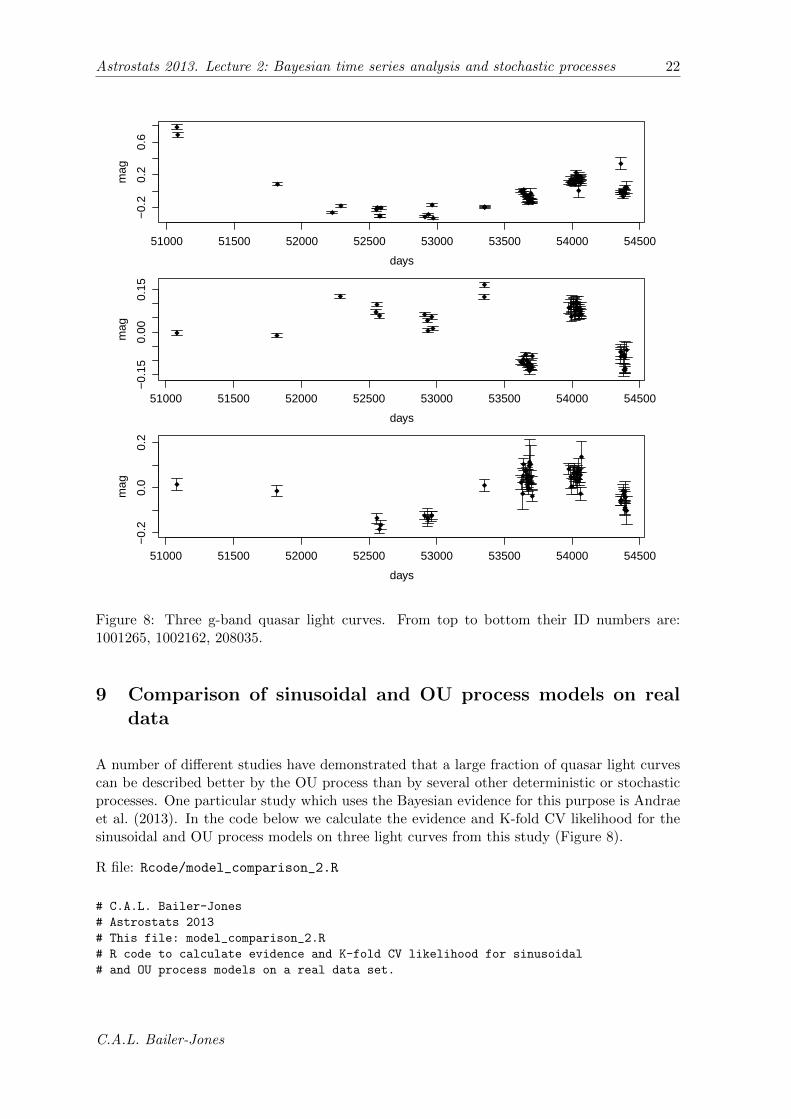
Figure 8: Three g-band quasar light curves. From top to bottom their ID numbers are:1001265, 1002162, 208035.

9 Comparison of sinusoidal and OU process models on realdata

A number of different studies have demonstrated that a large fraction of quasar light curvescan be described better by the OU process than by several other deterministic or stochasticprocesses. One particular study which uses the Bayesian evidence for this purpose is Andraeet al. (2013). In the code below we calculate the evidence and K-fold CV likelihood for thesinusoidal and OU process models on three light curves from this study (Figure 8).

R file: Rcode/model_comparison_2.R


# Astrostats 2013

# This file: model_comparison_2.R

# R code to calculate evidence and K-fold CV likelihood for sinusoidal

# and OU process models on a real data set.

C.A.L. Bailer-Jones


library(gplots) # for plotCI()

source("sinusoidal.R")

source("OUprocess.R")

source("monte_carlo.R")

source("kfoldCV.R")

########## Read in data

# Files:

#obsdata <- read.table("../data/g-band-LC_1001265.dat", header=FALSE)

#obsdata <- read.table("../data/g-band-LC_1002162.dat", header=FALSE)

obsdata <- read.table("../data/g-band-LC_208035.dat", header=FALSE)

# Models assumes data are zero mean


plotCI(obsdata[,1], obsdata[,3], uiw=obsdata[,4], err="y", xlab="time", ylab="signal",

pch=18, type="n", gap=0, sfrac=0.01)

########## Set priors and fixed parameters

zrange <- diff(range(obsdata[,3]))

alphaSinusoidal <- 0.5*c(zrange/2, zrange/2, 1/1000) # c(sd_a1, sd_a2, scale_freq)

#

ouprocFixed <- c(obsdata[,3], 0) # c(zstartmean, zstartsd)

tscale <- diff(range(obsdata[,1]))/10

alphaOUprocess <- 0.5*c(2*var(obsdata[,3])/tscale, tscale) # c(scale_diffcon, scale_relax)

########## Calculate evidences

set.seed(100)

# sinusoidal model

Nsamp <- 1e4

priorSamples <- sampleprior.sinusoidal(Nsamp, alphaSinusoidal)

logLike <- vector(length=Nsamp)

for(i in 1:Nsamp) {

logLike[i] <- loglike.sinusoidal(priorSamples[i,], obsdata)

}

evSM <- mean(10^logLike)

# OUprocess

Nsamp <- 1e4

priorSamples <- sampleprior.OUprocess(Nsamp, alphaOUprocess)

logLike <- vector(length=Nsamp)

for(i in 1:Nsamp) {

logLike[i] <- loglike.OUprocess(priorSamples[i,], obsdata, ouprocFixed)

}

evOU <- mean(10^logLike)

#

cat("Bayes factor [OUprocess/sinusoidal] = ", evOU/evSM, "\n")

cat("log10 Bayes factor [OUprocess - sinusoidal] = ", log10(evOU/evSM), "\n")

cat("log10 Evidences [OUprocess, sinusoidal] = ", log10(evOU), log10(evSM), "\n")

########## Calculate K-fold CV likelihoods

set.seed(100)

# sinusoidal model: c(a1, a2, freq)

sampleCov <- make.covariance.matrix(sampleSD=alphaSinusoidal/50, sampleCor=0)

C.A.L. Bailer-Jones


thetaInit <- alphaSinusoidal

kcvSM <- kfoldcv(Npart=10, obsdata=obsdata, logpost=logpost.sinusoidal,

loglike=loglike.sinusoidal, sampleCov=sampleCov, thetaInit=thetaInit,

Nburnin=1e3, Nsamp=1e4, alpha=alphaSinusoidal)

# OUprocess model: c(diffcon, relax)

sampleCov <- make.covariance.matrix(sampleSD=alphaOUprocess, sampleCor=0)

thetaInit <- alphaOUprocess

kcvOU <- kfoldcv(Npart=10, obsdata=obsdata, logpost=logpost.OUprocess,

loglike=loglike.OUprocess, sampleCov=sampleCov, thetaInit=thetaInit,

Nburnin=1e3, Nsamp=1e4, ouprocFixed=ouprocFixed, alpha=alphaOUprocess)

#

cat("log10 K-fold CV likelihood [OUprocess, sinusoidal]", kcvOU, kcvSM, "\n")

cat("Difference log10 K-fold CV likelihood [OUprocess - sinusoidal]", kcvOU - kcvSM, "\n")

######### Calculate posterior PDFs

# should really check the MCMC in the K-fold CV likelihood by plotting samples and

# posterior PDFs for the data partitions used there. But get a good idea by sampling

# the whole data set, as done here.

# sinusoidal model: c(a1, a2, freq)

sampleCov <- make.covariance.matrix(sampleSD=alphaSinusoidal/25, sampleCor=0)

thetaInit <- alphaSinusoidal

postSamp <- metrop(func=logpost.sinusoidal, thetaInit=thetaInit, Nburnin=1e3,


obsdata=obsdata, alpha=alphaSinusoidal)

parnames <- c("a1", "a2", "freq")






}

10 Exercises

R code to help you perform these exercises has been supplied above in the relevant sections.Recall that the analyses above assume the data to have zero mean signal, so you’ll need tosubtract the mean (even if you generate a finite amount of data from a zero mean process).

1. Sinusoidal model 1. Simulate data from a sinusoidal model (equation 2) and addsome Gaussian noise (see section 4). Calculate and plot the Schuster periodogram(equation 21) as well as the (unnormalized) log posterior PDF over frequency (i.e.the Bayesian periodogram), for the two cases of known common noise (equation 20)and unknown noise (equation 26). Experiment with changing the amount of data, theamplitudes and the frequency in relation to the time span.

2. Sinusoidal model 2. Taking one of your noisy simulated sinusoidal data sets, usean MCMC algorithm to infer the model parameters (i.e. sample the posterior). (Seesection 4.)

C.A.L. Bailer-Jones


3. OU process 1. Using the code in section 8, simulate data from an OU process usingthe update equations 41 and 42 for specific values of the two model parameters, τ andc. Get a feel for how changing the parameters alters the properties of the process theparameters. For fixed parameters, also get a feel for how much the time series changesjust by changing the random number seed. (In addition to plotting the generated datapoints, plot the distributions – as mean and error bar – of the update equations.)

4. OU process 2. Simulate data from an OU process as in the previous exercise andadd some Gaussian noise. Using the code in section 8, infer the model parameters (i.e.sample the posterior).

5. Astronomical variability. Look at the astronomical time series provided and exam-ined in section 9. Visual inspection suggests this may show periodic variability, butmaybe a stochastic model explains the data better? Adopting suitable priors, use theBayesian evidence to compare a periodic model with an OU process model. (You mayalso use the K-fold CV likelihood, but it can take a while to run). Infer the posteriorPDFs over the parameters of the two models to check whether there is a dominantsolution. For comparison you may also want to calculate the various periodograms) forthe two models, discussed in section 3.

A Further reading

Andrae R., Kim D.-W., Bailer-Jones C.A.L., 2013, Assessment of stochastic and deterministicmodels of 6 304 quasar lightcurves from SDSS Stripe 82, A&A in presshttp://arxiv.org/abs/1304.2863

Bailer-Jones C.A.L., 2012, A Bayesian method for the analysis of deterministic and stochastictime series, A&A 546, A89See http://www.mpia.de/~calj/ctsmod.html for more information and software

Bretthorst G.L., 1998, Bayesian spectrum analysis and parameter estimation, Lecture notesin statistics vol. 48, SpringerOut of print, but available from http://http://bayes.wustl.edu/glb/book.pdf

Gardiner C., 2009, Stochastic methods, Springer, 4th editionA definitive work, but is hard going after the first few chapters

Gillespie D.T., 1996, Exact numerical simulation of the Ornstein–Uhlenbeck process and itsintegral, Phys. Rev. E, 54, 2084

Gillespie D.T., 1996b, The mathematics of Brownian motion and Johnson noise, Am. J.Phys. 64, 225A nice introduction to stochastic processes

Gregory P.C., 2005, Bayesian logical data analysis for the physical sciences, Cambridge Uni-versity PressChapter 13 is on spectral analysis

Scott M., 2011, Applied stochastic processes in science and engineering, unpublished book,http://www.math.uwaterloo.ca/~mscott/Little_Notes.pdf

C.A.L. Bailer-Jones

http://arxiv.org/abs/1304.2863

http://www.mpia.de/~calj/ctsmod.html

http://http://bayes.wustl.edu/glb/book.pdf

http://www.math.uwaterloo.ca/~mscott/Little_Notes.pdf


B R functions for the sinusoidal model

R file: Rcode/sinusoidal.R


# Astrostats 2013

# This file: sinusoidal.R

# R functions related to the single frequency sinusoidal model

# An event is described by a 4 element vector c(s, s.sd, y, y.sd)

# where s is the time and y is the signal and s.sd and y.sd their

# uncertainties, respectively.

# Nevents is the number of events

# obsdata is a matrix of Nevents (rows) and 4 ordered columns c(s, s.sd, y, y.sd)

# Given sinmod and times eventTimes (vector), generate data from a sinusoidal model,

# optionally with additional Gaussian measurement noise of standard deviation ysigma.

# sigma can be a vector of length eventTimes, or a scalar. Default value is zero.

# Return in format obsdata.

gen.sinusoidal <- function(sinmod, eventTimes, ysigma=0) {

Nevents <- length(eventTimes)

obsdata <- matrix(data=0, nrow=Nevents, ncol=4)

obsdata[,1] <- eventTimes

obsdata[,2] <- 0

obsdata[,4] <- ysigma

omegat <- 2*pi*sinmod$freq*obsdata[,1]

obsdata[,3] <- sinmod$a1*cos(omegat) + sinmod$a2*sin(omegat)

obsdata[,3] <- obsdata[,3] + rnorm(Nevents, mean=0, sd=obsdata[,4])

return(obsdata)

}

# Plot obsdata, and optionally overplot a sinusoidal model with parameters sinmod.

# trange=c(tmin,tmax) can be supplied, otherwise (if it’s NULL) is calculated from the data.

# If ploterr=TRUE, plot error bars.

# If fname is supplied, save the plot in a PDF with this name.

oplot.obsdata.sinusoidal <- function(obsdata, sinmod=NULL, trange=NULL,

ploterr=TRUE, fname=NULL) {

library(gplots)

if(!is.null(fname)) pdf(fname, width=6, height=5)

par(mfrow=c(1,1), mgp=c(2.0,0.8,0), mar=c(3.5,4.0,1.0,1.0), oma=c(0,0,2.0,0), cex=1.2)

if(is.null(trange)) {

trange <- range(c(obsdata[,1]+obsdata[,2], obsdata[,1]-obsdata[,2]))

}

if(!is.null(sinmod)) {

tmod <- seq(from=min(trange), to=max(trange), length.out=1e3)

omegat <- 2*pi*sinmod$freq*tmod

ymod <- sinmod$a1*cos(omegat) + sinmod$a2*sin(omegat)

ymin <- min(ymod, obsdata[,3]-obsdata[,4])

ymax <- max(ymod, obsdata[,3]+obsdata[,4])

} else {

ymin <- min(obsdata[,3]-obsdata[,4])

ymax <- max(obsdata[,3]+obsdata[,4])

}

plot(obsdata[,1], obsdata[,3], xlim=trange, ylim=c(ymin,ymax), pch=18,

C.A.L. Bailer-Jones


xlab="time", ylab="signal")

if(ploterr) plotCI(obsdata[,1], obsdata[,3], uiw=obsdata[,4], err="y", type="n",

gap=0, sfrac=0.01, add=TRUE)

if(!is.null(sinmod)) {

lines(tmod, ymod, col="red")

}

mtext("measured = black, model = red", padj=-1)

if(!is.null(fname)) dev.off()

}

# Calculate the Schuster periodogram of obsdata at NFreq uniformly spaced

# frequencies between minFreq and maxFreq.

# Plot this as well as the unnormalized posterior assuming

# (1) a common sigma for all the data equal to the mean of obsdata[,4].

# (2) sigma is unknown

# as well as the other assumptions noted in the script for the

# approximations to hold.


schuster <- function(obsdata=obsdata, minFreq=NULL, maxFreq=NULL, NFreq=NULL, fname=NULL) {

cat("mean, sd of data =", mean(obsdata[,3]), sd(obsdata[,3]), "\n")

J <- nrow(obsdata)

sampFreq <- seq(from=minFreq, to=maxFreq, length.out=NFreq)

schuster <- vector(mode="numeric", length=length(sampFreq))

for(f in 1:length(sampFreq)) {

omegat <- 2*pi*sampFreq[f]*obsdata[,1]

R <- sum(obsdata[,3]*cos(omegat))

I <- sum(obsdata[,3]*sin(omegat))

schuster[f] <- (R^2 + I^2)/J

}

schusterNorm <- schuster/( sum(schuster)*(maxFreq-minFreq)/NFreq ) # set area to unity

#


par(mfrow=c(3,1), mar=c(0.5,3.5,0,0), oma=c(3.0,0,1,1), mgp=c(2.0,0.6,0), cex=1.1)

plot(sampFreq, schusterNorm, xaxt="n", ylab="power (normalized)", type="l")

text(max(sampFreq), 0.9*max(schusterNorm), "Schuster periodogram", pos=2)

# posterior periodogram with known common sigma

logpost <- (1/log(10))*schuster/mean(obsdata[,4])^2

plot(sampFreq, logpost, xaxt="n", ylab="log10post", type="l")

text(max(sampFreq), 0.9*max(logpost), "assuming common sigma", pos=2)

# posterior periodogram with unknown sigma

# print(sum(obsdata[,3]^2)/2 - schuster) # check: are always positive

posterior <- (sum(obsdata[,3]^2)/2 - schuster)^((2-J)/2)

plot(sampFreq, log10(posterior), ylab="log10post", type="l")

text(max(sampFreq), 0.7*max(log10(posterior)), "assuming unknown sigma", pos=2)

#

mtext("frequency", side=1, line=1.5, outer=TRUE, cex=1.1)


}

# Return log10(unnormalized posterior) of the sinusoidal model

# (see notes on the functions called)

logpost.sinusoidal <- function(theta, obsdata, alpha, ind=NULL) {

logprior <- logprior.sinusoidal(theta, alpha)

if(is.finite(logprior)) { # only evaluate model if parameters are sensible

return( loglike.sinusoidal(theta, obsdata, ind) + logprior )

C.A.L. Bailer-Jones


} else {

return(-Inf)

}

}

# Return log10(likelihood) of the sinusoidal model on rows ind of

# obsdata (to within an additive constant)

# with parameters theta = c(a1, a2, freq)

# ... is needed to pick up the unwanted alpha passed by kfoldcv(),

loglike.sinusoidal <- function(theta, obsdata, ind=NULL, ...) {

if(is.null(ind)) ind <- 1:nrow(obsdata)

omegat <- 2*pi*theta[3]*obsdata[ind,1]

modpred <- theta[1]*cos(omegat) + theta[2]*sin(omegat)

logEventLike <- (1/log(10))*dnorm(x=obsdata[ind,3], mean=modpred,

sd=sqrt(obsdata[ind,4]), log=TRUE)

return( sum(logEventLike) )

}

# Return log10(unnormalized prior) of the sinusoidal model

# with parameters theta = c(a1, a2, freq) and selected prior

# hyperparameters alpha

logprior.sinusoidal <- function(theta, alpha) {

a1Prior <- dnorm(x=theta[1], mean=0, sd=alpha[1])

a2Prior <- dnorm(x=theta[2], mean=0, sd=alpha[2])

freqPrior <- dgamma(x=theta[3], shape=1.5, scale=alpha[3])

return( sum(log10(a1Prior), log10(a2Prior), log10(freqPrior)) )

}

# return Nsamp samples from prior

# (is consistent with logprior.sinusoidal)

sampleprior.sinusoidal <- function(Nsamp, alpha) {

a1 <- rnorm(n=Nsamp, mean=0, sd=alpha[1])

a2 <- rnorm(n=Nsamp, mean=0, sd=alpha[2])

freq <- rgamma(n=Nsamp, shape=1.5, scale=alpha[3])

return(cbind(a1, a2, freq))

}

C R functions for the OU process

R file: Rcode/OUprocess.R


# Astrostats 2013

# This file: OUprocess.R

# R functions related to the OU process

# An event is described by a 4 element vector c(s, s.sd, y, y.sd)

# where s is the time and y is the signal and s.sd and y.sd their

# uncertainties, respectively.

# Nevents is the number of events

# obsdata is a matrix of Nevents (rows) and 4 ordered columns c(s, s.sd, y, y.sd)

# ouproc is a named list of the parameters of the OU process

C.A.L. Bailer-Jones


# ouproc = list(diffcon, relax, zstartmean, zstartsd)

# zstartmean and zstartsd are the initial conditions.

# Given ouproc and times eventTimes (vector), generate data from an OU process

# using the update equations.

# If ysigma>0 add Gaussian measurement noise with this standard deviation.

# ysigma can be a vector of length eventTimes, or a scalar. Default value is zero.

# Return a two element list:

# obsdata

# procDist, a dataframe with Nevents rows and 2 columns:

# mean and variance of the process itself at each time step

gen.OUprocess <- function(ouproc, eventTimes, ysigma=0) {

Nevents <- length(eventTimes)

obsdata <- matrix(data=0, nrow=Nevents, ncol=4)

zMean <- vector(mode="numeric", length=Nevents)

zVar <- vector(mode="numeric", length=Nevents)

obsdata[,1] <- eventTimes

obsdata[,2] <- 0

zMean[1] <- ouproc$zstartmean

zVar[1] <- ouproc$zstartsd

obsdata[1,3] <- ouproc$zstartmean + rnorm(1, mean=0, sd=ouproc$zstartsd)

for(j in 2:Nevents) {

nu <- exp(-(obsdata[j,1]-obsdata[j-1,1])/ouproc$relax)

Vz <- (ouproc$diffcon*ouproc$relax/2)*(1-nu^2)

zMean[j] <- obsdata[j-1,3]*nu

zVar[j] <- Vz

obsdata[j,3] <- rnorm(1, mean=zMean[j], sd=sqrt(zVar[j]))

}

if(ysigma>0) { # add measurement noise

obsdata[,4] <- ysigma

obsdata[,3] <- obsdata[,3] + rnorm(Nevents, mean=0, sd=obsdata[j,4])

}

return(list(obsdata=obsdata, procDist=data.frame(zMean=zMean, zVar=zVar)))

}

# Plot obsdata, and optionally overplot either (if defined)

# (1) points with mean and variance given by procDist, or

# (2) predicted priors of an OU process evaluated on these data with parameters ouproc.

# If both are defined then only (1) is plotted. (This will usually be used to

# plot the mean and sd of the update formula used to generate obsdata.)

# The data are plotted in black, procDist in magenta, the predicted priors in red.

# trange=c(tmin,tmax) can be supplied, otherwise (if it’s NULL) is calculated from the data.

# If ploterr=TRUE, plot error bars on the data.


# NOTE: This will give warnings if the error bars are too small to plot

oplot.obsdata.OUprocess <- function(obsdata, procDist=NULL, ouproc=NULL, trange=NULL,

ploterr=TRUE, fname=NULL) {

library(gplots)


if(is.null(trange)) {

trange <- range(c(obsdata[,1]+obsdata[,2], obsdata[,1]-obsdata[,2]))

}

if(!is.null(ouproc)) {

procParam <- eval.OUprocess(ouproc, obsdata)

}

C.A.L. Bailer-Jones


if(!is.null(procDist)) {

procParam <- procDist

}

par(mfrow=c(1,1), mgp=c(2.0,0.8,0), mar=c(3.5,3.5,1.0,1.0), oma=c(0,0,1,0), cex=1.1)

if(!is.null(procParam)) {

ymin <- min(c(procParam$zMean-sqrt(procParam$zVar), obsdata[,3]-obsdata[,4]))

ymax <- max(c(procParam$zMean+sqrt(procParam$zVar), obsdata[,3]+obsdata[,4]))

} else {

ymin <- min(obsdata[,3]-obsdata[,4])

ymax <- max(obsdata[,3]+obsdata[,4])

}

plot(obsdata[,1], obsdata[,3], xlim=trange, ylim=c(ymin,ymax), pch=18,

xlab="time", ylab="signal")

if(ploterr) plotCI(obsdata[,1], obsdata[,3], uiw=obsdata[,4], err="y", type="n",

gap=0, sfrac=0.01, add=TRUE)

if(!is.null(procDist)) {

points(obsdata[,1], procDist$zMean, pch=8, col="magenta")

plotCI(obsdata[,1], procDist$zMean, uiw=sqrt(procDist$zVar), err="y", type="n",

col="magenta", gap=0, sfrac=0.01, add=TRUE)

}

if(!is.null(ouproc) && is.null(procDist)) {

points(obsdata[,1], procParam$zMean, pch=8, col="red")

plotCI(obsdata[,1], procParam$zMean, uiw=sqrt(procParam$zVar), err="y", type="n",

col="red", gap=0, sfrac=0.01, add=TRUE)

}

mtext("measured = black, true process = magenta, model prior = red", padj=-1)


}

# Evaluate an OU process of given parameters using given obsdata.

# Specifially, return a ncol(obsdata) x 2 dataframe with named columns

# zMean and zVar which give the mean and variance of the prior PDF

# of the OU process variable at each event.

# Note: probably slower than it should be due to presence of loop

eval.OUprocess <- function(ouproc, obsdata) {

Nevents <- nrow(obsdata)

zMean <- vector(mode="numeric", length=Nevents)

zVar <- vector(mode="numeric", length=Nevents)

j <- 1

zMean[j] <- ouproc$zstartmean

zVar[j] <- ouproc$zstartsd^2

for(j in 1:Nevents) {

if(j > 1) {

# warning: divide by zero if relax=0 (controlled by prior)

nu <- exp(-(obsdata[j,1]-obsdata[j-1,1])/ouproc$relax)

Vz <- (ouproc$diffcon*ouproc$relax/2)*(1-nu^2)

zMean[j] <- zMeanPost*nu # + ouproc$offset*(1-nu)

zVar[j] <- zVarPost*nu^2 + Vz

}

if(j < Nevents) { # calculate posterior

ysigsq <- obsdata[j,4]^2

denom <- ysigsq + zVar[j]

if(denom==0) { # controlled by data/prior

stop("Both ysigsq and zVar are zero, so posterior moments are undefined")

}

C.A.L. Bailer-Jones


zMeanPost <- (obsdata[j,3]*zVar[j] + zMean[j]*ysigsq)/denom

zVarPost <- zVar[j]*ysigsq/denom

}

}

return(data.frame(zMean=zMean, zVar=zVar))

}

# Return log10(unnormalized posterior) of the OU process

# (see notes on functions called)

logpost.OUprocess <- function(theta, obsdata, ouprocFixed, alpha, ind=NULL) {

logprior <- logprior.OUprocess(theta, alpha)

if(is.finite(logprior)) { # only evaluate model if parameters are sensible

return( loglike.OUprocess(theta, obsdata, ouprocFixed, ind) + logprior )

} else {

return(-Inf)

}

}

# Return log10(likelihood) of the OU process defined by parameters

# theta = c(diffcon, relax) and ouprocFixed = c(zstartmean, zstartsd)

# for events ind in the time series obsdata (to within an additive

# constant). We require the full set of data in order to propagate the

# estimates of the process parameters along the chain of

# events. However, the likelihood is calculated and returned only for

# the events specified in ind. (This can be used for calculating the

# k-fold CV likelihood, for example.) If ind=NULL (the default), the

# likelihood for all the data is calculated.

# ... is needed to pick up the unwanted alpha passed by kfoldcv().

# Note: Function is much slower than other loglike functions, presumably

# due to eval.OUprocess()

loglike.OUprocess <- function(theta, obsdata, ouprocFixed, ind=NULL, ...) {

if(is.null(ind)) ind <- 1:nrow(obsdata)

ouproc <- list(diffcon=theta[1], relax=theta[2], zstartmean=ouprocFixed[1],

zstartsd=ouprocFixed[2])

procParam <- eval.OUprocess(ouproc, obsdata)

yMean <- procParam$zMean

yVar <- obsdata[,4]^2 + procParam$zVar

logEventLike <- (1/log(10))*dnorm(x=obsdata[ind,3], mean=yMean[ind],

sd=sqrt(yVar[ind]), log=TRUE)

return( sum(logEventLike) )

}

# Return log10(unnormalized prior) unnormalized prior of the OU process

# with parameters theta = c(diffcon, relax) and selected prior

# hyperparameters alpha.

# zstartmean and zstartsd are assumed fixed.

logprior.OUprocess <- function(theta, alpha) {

diffconPrior <- dgamma(x=theta[1], shape=1.5, scale=alpha[1])

relaxPrior <- dgamma(x=theta[2], shape=1.5, scale=alpha[2])

return( sum(log10(diffconPrior), log10(relaxPrior)) )

}

# return Nsamp samples from prior

# (is consistent with logprior.OUprocess)

sampleprior.OUprocess <- function(Nsamp, alpha) {

C.A.L. Bailer-Jones


diffcon <- rgamma(n=Nsamp, shape=1.5, scale=alpha[1])

relax <- rgamma(n=Nsamp, shape=1.5, scale=alpha[2])

return(cbind(diffcon, relax))

}

D Spectral analysis

D.1 General concepts

The auto-covariance function of the signal z(t) is auto-covariance

C(t′) = limT→∞

1

T

∫ T

0z(t)z(t+ t′) dt = 〈z(t)z(t+ t′)〉 . (49)

If z(t) is stationary, then the auto-covariance is independent of t.

The power spectrum of a stationary process z(t) is defined as powerspectrum

S(ω) = limT→∞

1

2πT|φ(ω)|2 (50)

where φ(ω) is the Fourier transform of the signal

φ(ω) =

∫ T

−Tz(t)e−iωt dt . (51)

Taking the limit T →∞, it can then be shown that

S(ω) =1

π

∫ ∞−∞

C(t)e−iωt dt

=2

π

∫ ∞0

C(t) cos(ωt) dt (52)

the second line following by taking just the real part and with 0 < ω <∞, and

C(t) =

∫ ∞0

S(ω) cos(ωt) dω . (53)

This shows that the power spectrum is the Fourier transform (real part, positive frequencies)of the auto-covariance function, and is known as the Wiener–Khintchine theorem. Settingt′ = 0 in equation 49 and t = 0 in equation 53 we see that

〈z(t)2〉 =

∫ ∞0

S(ω) dω . (54)

Thus we see that the power spectrum, S(ω), is the portion of intensity of the signal withfrequencies between ω and ω + dω. Note that it gives the frequency spectrum of 〈z(t)2〉 andnot of z(t) itself.

Comparing equation 21 with equation 50 we see that the Schuster periodogram is a discreteapproximation of the power spectrum over a finite time scale.

C.A.L. Bailer-Jones


0 1 2 3 4 5

0.00

0.10

0.20

0.30

frequency, w / radians

pow

er, S

(w)

−4 −2 0 2 4

−8

−6

−4

−2

log(w)

log(

S)

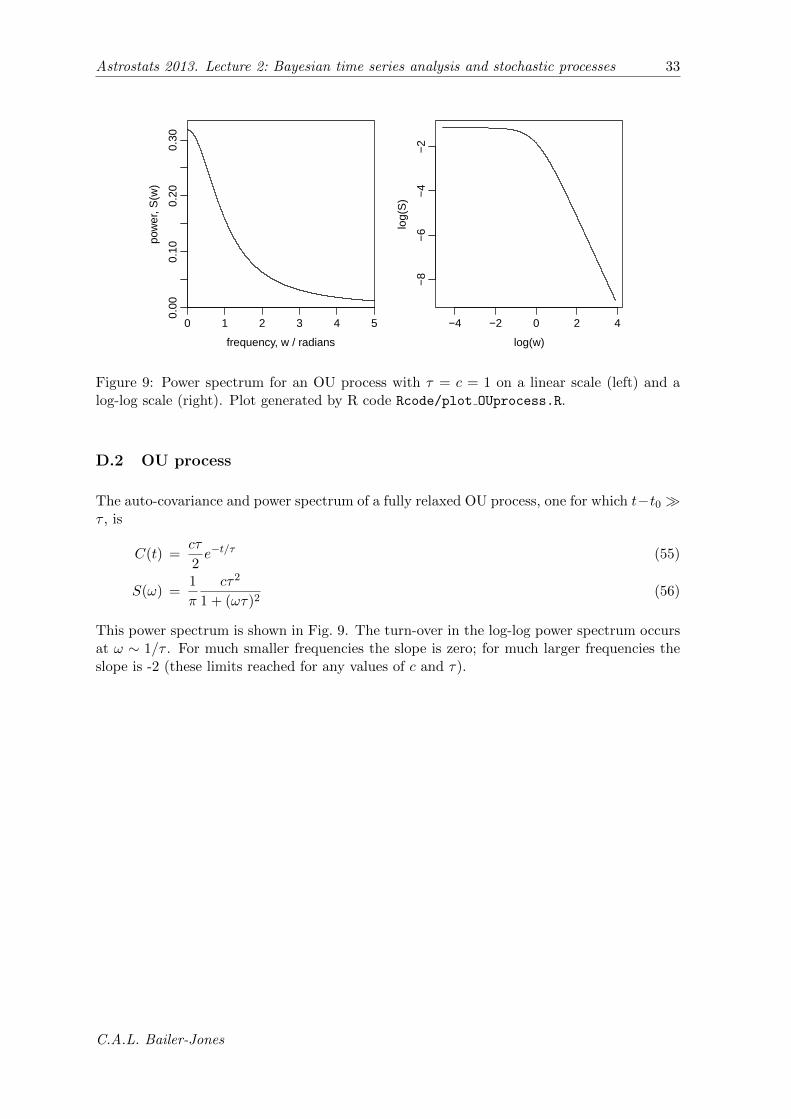
Figure 9: Power spectrum for an OU process with τ = c = 1 on a linear scale (left) and alog-log scale (right). Plot generated by R code Rcode/plot OUprocess.R.

D.2 OU process

The auto-covariance and power spectrum of a fully relaxed OU process, one for which t−t0 �τ , is

C(t) =cτ

2e−t/τ (55)

S(ω) =1

π

cτ2

1 + (ωτ)2(56)

This power spectrum is shown in Fig. 9. The turn-over in the log-log power spectrum occursat ω ∼ 1/τ . For much smaller frequencies the slope is zero; for much larger frequencies theslope is -2 (these limits reached for any values of c and τ).

C.A.L. Bailer-Jones

astrostats 2013 lecture 2 bayesian time series analysis and stochastic...

Documents