AFRL-IF-RS-TR-2006-16 Final Technical Report January 2006 ASSOCIATIVE MEMORY HARDWARE ELEMENTS FOR COGNITIVE SYSTEMS

Saffron Technology, Inc.

APPROVED FOR PUBLIC RELEASE; DISTRIBUTION UNLIMITED.

AIR FORCE RESEARCH LABORATORY INFORMATION DIRECTORATE

ROME RESEARCH SITE ROME, NEW YORK

STINFO FINAL REPORT

This report has been reviewed by the Air Force Research Laboratory, Information Directorate, Public Affairs Office (IFOIPA) and is releasable to the National Technical Information Service (NTIS). At NTIS it will be releasable to the general public, including foreign nations. AFRL-IF-RS-TR-2006-16 has been reviewed and is approved for publication APPROVED: /s/

CHRISTOPHER FLYNN Project Engineer

FOR THE DIRECTOR: /s/

JAMES A. COLLINS Deputy Chief, Advanced Computing Division Information Directorate

REPORT DOCUMENTATION PAGE Form Approved

OMB No. 074-0188 Public reporting burden for this collection of information is estimated to average 1 hour per response, including the time for reviewing instructions, searching existing data sources, gathering and maintaining the data needed, and completing and reviewing this collection of information. Send comments regarding this burden estimate or any other aspect of this collection of information, including suggestions for reducing this burden to Washington Headquarters Services, Directorate for Information Operations and Reports, 1215 Jefferson Davis Highway, Suite 1204, Arlington, VA 22202-4302, and to the Office of Management and Budget, Paperwork Reduction Project (0704-0188), Washington, DC 20503 1. AGENCY USE ONLY (Leave blank)

2. REPORT DATEJANUARY 2006

3. REPORT TYPE AND DATES COVERED Final Sep 2004 – May 2005

4. TITLE AND SUBTITLE ASSOCIATIVE MEMORY HARDWARE ELEMENTS FOR COGNITIVE SYSTEMS

6. AUTHOR(S) Manuel Aparicio

5. FUNDING NUMBERS C - FA8750-04-C-0245 PE - 62702F PR - 459T TA - CS WU - TC

7. PERFORMING ORGANIZATION NAME(S) AND ADDRESS(ES) Saffron Technology, Inc. 1600 Perimeter Park Drive, Suite 150 Morrisville North Carolina 27560-5421

8. PERFORMING ORGANIZATION REPORT NUMBER

N/A

9. SPONSORING / MONITORING AGENCY NAME(S) AND ADDRESS(ES) Air Force Research Laboratory/IFTC 525 Brooks Road Rome New York 13441-4505

10. SPONSORING / MONITORING AGENCY REPORT NUMBER

AFRL-IF-RS-TR-2006-16

11. SUPPLEMENTARY NOTES AFRL Project Engineer: Christopher Flynn/IFTC/(315) 330-3249 Christopher.Flynn@rl.af.mil

12a. DISTRIBUTION / AVAILABILITY STATEENT APPROVED FOR PUBLIC RELEASE; DISTRIBUTION UNLIMITED.

12b. DISTRIBUTION CODE

13. ABSTRACT (Maximum 200 Words) The effort focused on investigating cognitive computer architectural designs using associated memory hardware elements.

15. NUMBER OF PAGES106

14. SUBJECT TERMS Associative Memory, Cognitive Computing

16. PRICE CODE

17. SECURITY CLASSIFICATION OF REPORT

UNCLASSIFIED

18. SECURITY CLASSIFICATION OF THIS PAGE

UNCLASSIFIED

19. SECURITY CLASSIFICATION OF ABSTRACT

UNCLASSIFIED

20. LIMITATION OF ABSTRACT

ULNSN 7540-01-280-5500 Standard Form 298 (Rev. 2-89)

Prescribed by ANSI Std. Z39-18 298-102

i

Table of Contents 1. Introduction..................................................................................................................... 1

1.1 Real Intelligence ....................................................................................................... 1 1.2 Scope of work ........................................................................................................... 3 1.3 Outline of Report ...................................................................................................... 4

2. Building Block Algorithm .............................................................................................. 5 2.1 Memory-based Reasoning ........................................................................................ 5 2.2 Memory Scalability................................................................................................... 6 2.3 External Context ....................................................................................................... 7 2.4 Internal Attributes ..................................................................................................... 9 2.5 Association Matrices............................................................................................... 10 2.6 Segment Structure................................................................................................... 13 2.7 Bit Planes ................................................................................................................ 15 2.8 Sub-Segments ......................................................................................................... 16 2.9 Matrix Examples..................................................................................................... 18 2.10 Virtual Store.......................................................................................................... 20

3. VHDL Design ............................................................................................................... 22 3.1 Approach and Challenges ....................................................................................... 22

3.1.1 Existence matrix............................................................................................... 22 3.1.2 Context Size ..................................................................................................... 22 3.1.3 Raw counts....................................................................................................... 23 3.1.4 Atom-based Interface....................................................................................... 23

3.2 Overall Architecture................................................................................................ 24 3.2.1 Associative Memory Entity ............................................................................. 24 3.2.2 Persistence Entity............................................................................................. 25 3.2.3 Top-Level Schematic ....................................................................................... 26

3.3 Large Matrix Design ............................................................................................... 27 3.3.1 Naïve Crossbar Architecture............................................................................ 27 3.3.2 Large Matrix Architecture ............................................................................... 28 3.3.3 Blocks, Segments, and Bit Planes.................................................................... 28

3.4 Small Matrix Design ............................................................................................... 30 3.4.1 Naïve Small Matrix.......................................................................................... 30 3.4.2 Small Matrix Using Segments ......................................................................... 31

3.5 Simulation Outputs and Waveforms....................................................................... 32 3.5.1 File-Driven Test Bench.................................................................................... 33 3.5.2 Behavior of Memory System........................................................................... 33 3.5.3 Simulation Waveforms for Observe ................................................................ 34 3.5.4 Simulation Waveforms for Attribute Query .................................................... 36

3.6 Additional Considerations ...................................................................................... 38 4. Advanced Building Block Exploration......................................................................... 39

4.1 Synaptic Growth ..................................................................................................... 39 4.1 Coincidence Detection ............................................................................................ 40 4.2 Strength Sorting ...................................................................................................... 43 4.3 Affinity Sorting....................................................................................................... 48 4.4 Hierarchical Sharing ............................................................................................... 52

ii

4.5 Larger Scale ............................................................................................................ 55 4.6 Hardware Considerations........................................................................................ 57

4.6.1 Neuromorphic Chips........................................................................................ 57 4.6.2 Parallel sorting ................................................................................................. 59

5 Accomplishments and Lessons ...................................................................................... 61 5.1 Project Results ........................................................................................................ 61 5.2 Distributed Product Design..................................................................................... 62 5.3 Hardware Inexperience ........................................................................................... 62 5.4 Application Scope................................................................................................... 63 5.5 Theory Advancement.............................................................................................. 65

6 Future Directions ........................................................................................................... 66 6.1 Appliance Model..................................................................................................... 66 6.2 SBIR Continuation.................................................................................................. 68 6.3 Quantum Neurons ................................................................................................... 72

7 References...................................................................................................................... 74

List of Appendixes

Appendix A Associative Memory .................................................................................... 76 Appendix B Naïve Large Matrix ...................................................................................... 78 Appendix C Large Matrix................................................................................................. 80 Appendix D Naïve Small Matrix ...................................................................................... 84 Appendix E Small Matrix ................................................................................................. 88 Appendix F Matrix Type Utilities..................................................................................... 93 Appendix G Top Level ..................................................................................................... 95 Appendix H Persistence.................................................................................................... 97 Appendix I Testbench ....................................................................................................... 98

List of Figures Figure 1: Inspiration for dominant linearity in real dendritic neural structures.................. 1 Figure 2: Symmetric associative matrix of coincidence counts.......................................... 9 Figure 3: Atom table from external to internal attributes ................................................... 9 Figure 4: Virtual attribute addressing of Large Associative Matrix ................................. 11 Figure 5: Actual values within Large Association Matrix................................................ 11 Figure 7: Virtual list of segments in Large Matrix ........................................................... 14 Figure 8: List of actual segments that have association counts ........................................ 14 Figure 9: List of single segment in Small Matrix ............................................................. 15 Figure 10: Sub-segment structure of map and data elements ........................................... 17 Figure 11: Entire matrix structure from segments to bit planes to sub-segments............. 17 Figure 12: Repeated example of Large Matrix segment list............................................. 18 Figure 13: Structure of example segment down to actual data representation ................. 18 Figure 14: Another example segment down to actual data representation ....................... 19

iii

Figure 15: List of segments and all actual data representations ....................................... 19 Figure 16: Repeated example of single segment for Small Matrix .................................. 20 Figure 17: Structure of Small Matrix example down to actual data representation ......... 20 Figure 18: Structure of example segment down to actual data representation ................. 21 Figure 19: Symbol Schematic for Associative Memory Entity ........................................ 25 Figure 20: VHDL implementation of BasicFlash............................................................. 26 Figure 21: Complete Schematic of General Interface....................................................... 27 Figure 22: VHDL implementation of block and segment indices .................................... 29 Figure 23: Indexing structures for blocks and segments .................................................. 29 Figure 24: VHDL structures for segments and blocks...................................................... 30 Figure 25: Data Structures for Naïve Small Matrix Design ............................................. 31 Figure 26: Structure of testbench input file ...................................................................... 33 Figure 27: Finite State Machine Diagram......................................................................... 34 Figure 28: Waveform of Observe (part 1 of 2) ................................................................. 35 Figure 29: Waveform for Observe (part 2 of 2)................................................................ 35 Figure 30: Waveform for Imagine (part 1 of 2)................................................................ 37 Figure 31: Waveform for Imagine (part 2 of 2)................................................................ 37 Figure 32: Synaptic changes in long-term potentiation as the basis for learning ............. 40 Figure 33: Historical examples of crossbar for associative memory hardware ................ 41 Figure 34: Recent ideas for coincidence detection within dendrites and neurons............ 42 Figure 35: Arbitrary matrix and its row and column ....................................................... 44 Figure 36: Digital tomography and projection sorting .................................................... 44 Figure 37: Read operation on projections and sort order of maximal matrix................... 45 Figure 38: Matrix views and run lengths before and after strength sorting...................... 46 Figure 39: Strength sorting of Small Matrices.................................................................. 47 Figure 40: Matrix sorting as Traveling Sales Problem ..................................................... 48 Figure 41: Prior-Next counts as statistical affinity of terms to each other ....................... 50 Figure 42: Matrix views and run lengths before and after affinity sorting....................... 51 Figure 43: Affinity sorting of Small Matrices .................................................................. 51 Figure 44: Dendritic structure of neurons as linear segments arranged in a tree.............. 52 Figure 45: Hierarchical separation of common counts ..................................................... 53 Figure 46: Strength sorting and hierarchical grouping ..................................................... 54 Figure 47: Affinity sorting and hierarchical grouping...................................................... 54 Figure 48: Comparison of all sorting (solid line) and sharing (dotted line) cases............ 55 Figure 49: Larger sampling of affinity sorting (red) and sharing (green) methods .......... 56 Figure 50: Self-organization of receptor map based on swapping of “softwires”............ 57 Figure 51: LTP induced spine growth over minutes and hours following learning ......... 58 Figure 52: Small Matrix translation table for affinity-based sorting ................................ 59 Figure 53: Theory of Neural Structure based on some combination of sortings .............. 60 Figure 54: FPX Configuration for deep context processing at Internet rates ................... 69 Figure 55: Distributed hardware/software processors across by massive storage............ 71 Figure 56: Microtubule with electron switching and electro-isolated interior ................. 72

1

1. Introduction

1.1 Real Intelligence Saffron Technology was formed to build truly intelligent cognitive systems. Rejecting traditional artificial intelligence and even “neural networks” as little to do with real neural systems, Saffron was inspired by the power of real neural devices, which we believe to be very complex, highly-nonlinear, nano-computing devices. Specifically, we believe them to be associative memories. Figure 1 below (Segev, 1998) for example presents a number of different neural types, which all display a dendritic, tree-like structure. Overall, these structures are dominantly linear. The inspiration for Saffron to emulate such neurons as the fundamental building blocks of neuro-cogntive systems is this: how do such dominantly linear structures compute complex nonlinear associations? The answers must rest in some form of compression and partitioning of associative memories into such linear and dendritic structures. We believe that neurons have solved the “crossbar problem”. Naïve hardware implementations as associative matrices connect everything to everything else in a complete, geometric crossbar. In contrast, neural inputs are known to store associative strengths and to interact with each other, but there is no obvious crossbar in these devices.

Figure 1: Inspiration for dominant linearity in real dendritic neural structures

2

The history of “neural” networks has not appreciated this potential power of neural devices. In fact, the rebirth of neural networks in the 1980s was founded largely by the school of Parallel Distributed Processing (PDP). This approach (Rumelhart and McClelland, 1986) argued that neurons are slow, inaccurate, and otherwise weak computational units. The power of neural systems is provided in the massive numbers of such units. Weak neurons are “saved” only by massive parallelism of distributed representations. While such neuro-computations succeeded in many industries, beyond more traditional AI, the dismissal of neural complexities resulted in many limitations. Most of these traditional neural network models are highly-parametric, slow to learn, non-incremental, and subject to over-fitting. This is not how our brains work. Fortunately, there is now an increasing turn toward more realistic cognitive systems and more realistic neurons. There is also a growing belief that neurons are memories and that memory-based systems are the foundation of “real intelligence”. Most recently, Jeff Hawkins has popularized the trend toward such real, memory-based intelligence in his book, On Intelligence: How a new understanding of the brain will lead to the creation of truly intelligent machines (2004). Very much like Saffron’s concerns with compression as the way neurons represent nonlinear interactions within linear structures, Hawkins predicts that neurons must be capable of “coincidence detection on thin dendrites”. In other words, neurons are associative memories and these associations are represented within the thin, linear processes of each dendrite. Saffron’s current products are software systems relying on Von Neumann computing architectures, but Saffron believes that real neurons are physical devices and that more is to be gained by deeper understanding and emulation. In addition to increased scientific understanding, this is also likely to be a very large business and probably an entire new industry. To again reference Hawkins, he believes that associative memories are the fundamental unit of future cognitive systems: “One day more silicon will be devoted to associative memories than for any other purpose.” (“That’s not how my brain works”, MIT Technology Review, 1999). The work reported here, supported by AFRL, has moved Saffron closer to these goals. Saffron has an enormous lead in the underlying implementation and application of associative memories for a wide variety of problems. Our proof points range from powering the “World’s Best Spam Blocker” (PC User Magazine review of Electronic Learning Assistant, 2003) to uniquely solving the pains and failures of the intelligence community in alias detection and database disambiguation (Case Study, available from Saffron, for classified customer). Other applications include military logistics and ISR decision support systems using our memory-based, experience-based approach. However, Saffron’s products are currently 100% Java. In order to continue its scaling for the most difficult problems in national security and large enterprises generally, we need to move to more hardware-based “appliance” systems. From near term appliance models to the far term vision of associative memories embedded in every device, this AFRL

3

work initiated this new corporate direction. We made progress in the engineering of our systems in hardware as well as in further understanding of what real neurons might do.

1.2 Scope of work The project began by assuming two levels for defining a unified cognitive architecture:

• Building Block. In biological terms, this level assumes that the neuron is the fundamental computing device. Therefore, such a “building block” is singular. Unlike most data modeling techniques and the grab-bag of data mining techniques, each of which is appropriate for only one function, this building block is assumed to be universally powerful. This is in fact the case for Saffron’s software in that one underlying representation supports a large number of different inferential functions. The goal of the building block effort was to port Saffron’s software designs into VHDL. Also, hardware-based neurons might lead to further understanding of this universal cognitive device.

• Cognitive Constructs. Assuming the building block, the project had planned to demonstrate this building block within a small number of different cognitive constructs, also in VHDL hardware specifications. A wide number of such constructs can be enumerated. For example, many neural principles are now textbook cases (for instance, see the classic Principles of Neural Science by Kandel et al., 2000). Saffron also has developed a large number of associative memory “design patterns” that have served a number of different applications. The breadth of these principles and patterns across a range of applications already proves the universal nature of the building block, but the intention was to further describe these constructs in VHDL.

However, as specific application requirements for the cognitive constructs unfolded, they moved more towards general Information Management rather than specific embedded systems. Embedded systems will tend to use building blocks in dedicated ways that also require the Cognitive Construct to be embedded in hardware. For example, this work began with the development of an embedded design for Cognitive Maps with Unmanned Combat Air Vehicles (UCAV). A Cognitive Map is one such cognitive construct for representing external space and how to explore and navigate it using an internal memory. Given the requirements of on-board autonomy and real-time rates, such initial designs were intended for embedded systems of both the building block and cognitive constructs. Both AFRL Information Directorate interests and Saffron’s business interests redirected this work toward General Information Management. Based on Saffron’s experience, such general purpose applications require a more general purpose micro-processor to support a wider number of construct and application types, which should remain in software to maximize their flexibility and extension. For example, Saffron’s product design separates SaffronOne as a singular core engine used in many different ways. This core can be seen as the universal building block, while many information management applications that use it are more flexible and variable. Embedded systems remain as a large potential future of a hardware building block, but for the business of moving Saffron products to an appliance model, the SaffronOne

4

engine is the “hot spot” and would most benefit from hardware processing. As will be described in Future Directions, other current research in cognitive hardware platforms, which Saffron intends to work with, also provide for such software-hardware mixes. Therefore, only the Building Block itself was reasonable to port to VHDL as will also be described and became the greater focus on this effort overall. The project work evolved into two primary investigations, both around different aspects of the Building Block:

• Development of hardware from current methods. This portion of work was essentially a specification and porting exercise. Given Saffron’s current methods in software, much of this work and report is dedicated to specifying the core methods and then describing them in VHDL behavioral descriptions. Even though this effort did not drive down to RTL descriptions, this work and report serves to prove and communicate Saffron’s algorithms and possible hardware designs for subsequent synthesis and implementation.

• Research of neural devices for new methods. While Saffron has made much progress in its respect for neural inspiration, there is still an enormous gap between its current algorithms and the Holy Grail of what real neurons must be computing with much more power and elegance. From its inception, Saffron has implemented and explored a number of additional methods, with more or less success. This work was an opportunity to further explore such intriguing but still unknown methods within real neural devices. We failed to reach the big breakthrough of neural theory, but we did make great strides in some new methods that will be practical to both software and hardware implementations, although hardware is more clearly required for these additional methods and hints at the needs for a “neuromorphic” device.

1.3 Outline of Report This report is organized as follows:

• Building Block Algorithm. Describes the compression and partitioning algorithms for Saffron’s associative memory representation.

• VHDL Design. Describes the rationale, VHDL elements, and testbench and waveform proofs of the hardware design effort.

• Advanced Explorations. Describes new algorithms and results for further compression, including how these methods require hardware parallelism, perhaps based on message passing in real neurons.

• Accomplishments and Lessons. Summarizes progress made in VHDL development and algorithmic research, as well as discussion of failures and lessons learned.

• Future Directions. Discusses Saffron’s growing need for a hardware appliance and plans for continuing this work in an AFRL supported SBIR. Includes review of neural network quantum algorithms speculation about long-term future.

All VHDL code listings for several versions of the Building Block are included in an appendix. Although Cognitive Constructs were not explicitly pursued in VHDL, and therefore not a direct effort leading to any new accomplishments, a number of examples have been presented in prior reports to demonstrate how the memory-based building

5

block can in fact provide the core of a unified cognitive architecture, which remains as a continuing goal of this work and Saffron’s business interests.

2. Building Block Algorithm

2.1 Memory-based Reasoning Saffron provides a unified cognitive architecture based on memory. The neuron is understood to be the fundamental unit of nervous systems, and we propose that most neurons are memory devices. Some cognitive architectures are heterogeneous in that they assume a number of different functions, each provided by “black boxes” that utilize different methods, each method selected as best suited to its function. However, we believe that all human cognitive functions are implemented in memory-based neurons and that artificial cognitive architectures should also be homogeneous, in which all functions are provided by a single memory-based building block (in addition to auxiliary neurons for sensory transduction, mapping, etc). At a functional level, this approach to cognitive inferencing is called memory-based reasoning. In a classic article called, “Toward Memory-based Reasoning”, Stanfill and Waltz (1986) proposed that memories – not rules – should be the basis of cognitive systems. More recently, David Aha (1997) coined the term “lazy learning” to describe a class of machine learning techniques such as case-based, experience-based, and memory-based that are different from “eager learning” methods such as most neural networks and statistical methods which try to model data. For instance, whether using back propagation neural network or merely a polynomial line fitting formula, these methods seek to “fit” the data to a model. One problem is that such models are highly parametric and are subject to over-fitting. In contrast, lazy learners – like memories – are not fitting data to models but rather – like memories – are something between the raw data and such specific models. The addition of more experience does not lead to model degradation by over-fitting. More experience is simply more experience, which should be positive. As such, lazy learners follow a minimum commitment strategy for cognitive architectures. Whereas eager learning models are intended to provide one and only one function such as classification, segmentation, or pattern completion, the lazy learning approach can provide all such functions. Eager learners assume a single function at modeling time. They simply capture experience and then use this experience to answer one of many different questions put to them at run time. This flexibility of the memory-based approach can be demonstrated through a number of cognitive constructs, but all will be built with a single building block for providing such memory as a sort of neural unit. The Psychology of Learning and Memory is also informative. Even at a general textbook level, a great debate is described between “gradualist” versus “absolutist”. As in the common thinking about learning, change is thought to be gradual. Animals learn trial-after-trial and slowly improve in performing a given task. Likewise, neural processes as the basis of learning are sometimes thought to be slow and require repetition, such as by

6

the slow modification of synaptic weights. These assumptions have been adopted as common experience and are the basis for almost all traditional neural network models as well. Such as in the Perceptron “convergence” procedures, connection weighs are slowly changed through repeated presentations of the data – often through many repetitive “eons” across all the data – before the model has been fully trained. While there is evidence for such slow processes, both in psychological function and physiological structure, there is also equal evidence for an absolutist theory. Change is not slow but instantaneous. While the sigmoidal learning curve is demonstrated by virtually all learning experiments, this is seen as an artifact of the animal population: Each individual animal might learn the “right” answer on any given trial. For example, one learn which of many doors to go through to get the cheese, some animals will select and learn the right answer early, while others select and learn it later. Each animal might instantly learn the right choice based on the first success and use this memory perfectly for all subsequent trials; however, the statistical report of all animals in general will show a gradual learning curve across trials. Even within one individual when given complex tasks, it might take time to learn all the elements to perform the complete task, but discovery and memory for each element is instantaneous. It takes time to learn the task but not because all the “weights” are slowly changing. Each hypothesis-confirmation insight is instantaneously learned and remembered. Neurophysiology is also demonstrating how memory change, called Long Term Potentiation (LTP), can be caused by only one coincidence event, if the inputs are significant. In this light, Saffron’s approach is more toward instant memory rather than gradual learning. The objective is to store the observation of all coincidences as an associative matrix. While learning is slow and lossy, memory is instant and lossless.

2.2 Memory Scalability In order to provide a lossless memory, Saffron was founded on the belief that memory-based architectures must also shift from philosophies of abstraction to philosophies of compression. Traditional AI has often bemoaned the “curse of dimensionality” in the complexity of intelligent functions, whether logical or statistical. As such, rule-based heuristics and statistical techniques are lossy, model-based abstractions. Abstractions lose information and accuracy. For example, rules have problems in also covering exceptions to the rules, and market segmentations are very inaccurate in their predictions about each individual customer. In contrast, memories seek to be perfect memories in the recording of experience, but because such stores do not scale well, the curse of dimensionality has been addressed by two approaches:

• Compression. The first objective is to make the memories smaller. Smaller memories take less space and hold more information before resorting to abstraction and reduction. We seek lossless compressions. This eliminates a vast number of common compression methods that are useful for imaging and such, but do not serve well as an incremental memory. For many reasons, lossy presentations can never be truly incremental. General compression – even if lossless – also will not work for a memory. For example optimal, embedding

7

compressions like arithmetic coding do not provide a searchable compression. And more than merely being searchable, fast memories must allow random-access. The problem is akin to the compression of very large data cubes, which is notoriously difficult. Saffron’s multi-memory system is equivalent to an associative memory cube. However, incremental learning also requires that the compression allow for new data updates, which data cube compressions, even if randomly accessible, do not provide. In summary, memory compressions must be limited to lossless, random access, and incremental update methods.

• Partitioning. While Saffron began with the development of memory compressions, we also learned that compression alone is insufficient for massive scalability. As in a data cube, Saffron maintains a 2D associative matrix for a vast number of people, places, and things (elements of the third dimension). Even if one memory is compressed and small enough to be resident in RAM, the extremes of scaling push many matrices to be much larger than this. In any case, RAM must be managed across a vast number of memories. These scales also require partitioning. As such, Saffron includes the notion of an agent “perspective” for each plane of the data cube. Each person, place, or thing is modeled by its own associative matrix. Beyond this, even one very large matrix can require further partitioning and special organization. For instance, this problem is much like that a very large spatial modeling. Very large maps reside in persistence, but must be organized into partitions with co-localities so that queries efficiently fetch and use such organization. Associative memories are also 2D “maps” but their functions and queries are different and need different organization to optimize query (and update).

The follow sections provide explicit descriptions of Saffron’s compressions and partitions for associative memories. Other methods have also been used and some are further explored in Advanced Explorations, but the following provides the best description of the core product’s engineering.

2.3 External Context Saffron transforms the situation of the external world into “snapshots” defined as attribute:value, or key:value, vectors. For example, a transaction record is defined as a vector of field-name and field-value tuples. For unstructured sources such as news items of message cables, Saffron uses entity extractors to define the people, places, and things in each sentence for example. These “entities” along with surrounding keywords describe the context: how each entity is associated with surround entities and keywords. As a cognitive construct, each entity is modeled as a separate associative memory, but for now, assume that all the attribute-values of a record or sentence (or XML stanza) are treated as one context to be observed into one matrix. For example, if we have a sentence of “John and Mary went to New York.”, we would group all the concepts/entities within the sentence into a single Context. An entity extractor may extract the following key:value pairs.

8

Person: John Person: Mary City: New York All the key:value pairs of a Context are associated against each other. Therefore, a list of associations is created with Person: John <-> Person: Mary = 1 Person: John <-> City: New York = 1 Person: Mary <-> City: New York = 1 If another sentence is observed into the system, its associations are merged with earlier sentences. For example, “John and Mary live in Seattle”. An entity extractor may extract the following key:value pairs. Person: John Person: Mary City: Seattle. The new Context’s list of associations would be Person: John <-> Person: Mary = 1 Person: John <-> City: Seattle = 1 Person: Mary <-> City: Seattle = 1 Merging the two lists of associations would be Person: John <-> Person: Mary = 2 Person: John <-> City: New York = 1 Person: Mary <-> City: New York = 1 Person: John <-> City: Seattle = 1 Person: Mary <-> City: Seattle = 1 As more contexts are observed, the list of associations grows. As given associations are observed over and over again, the association count also grows. Obviously, as in Figure 2, a more useful way to view the list of associations would be in matrix form, where the key:value pairs are indices of the matrix. This matrix is called an association matrix, also known as a coincidence matrix.

9

Jo h n M a ry N ew Y o rk S e a ttle

Jo h n 2 1 1

M ary 2 1 1

N ew Y o rk 1 1

S e a ttle 1 1

Jo h n M a ry N ew Y o rk S e a ttle

Jo h n 2 1 1

M ary 2 1 1

N ew Y o rk 1 1

S e a ttle 1 1

Jo h nJo h n M a ryM a ry N ew Y o rkN ew Y o rk S e a ttleS e a ttle

Jo h nJo h n 22 11 11

M aryM ary 22 11 11

N ew Y o rkN ew Y o rk 11 11

S e a ttleS e a ttle 11 11

Figure 2: Symmetric associative matrix of coincidence counts The dimension of the association matrix grows at a O(N2)rate, where N is the number of key:value pairs. The counts themselves grow at an O(logO) rate, where O is the number of observations. Therefore the majority of this design is concerned with minimizing the N2 growth and capitalizing on the logO growth.

2.4 Internal Attributes The first step is to change the external key:value information into an internal representation. This allows for easier manipulation of the data. Every value for each “key” and “value” is mapped to a numerical number (also called an “atom”). Therefore the above example would be mapped to Figure 3:

Figure 3: Atom table from external to internal attributes

A t o m T a b l e ( V i r t u a l S t o r e )

p e r s o n 1

J o h n 2

A t t r K e y / V a l u e N N

M a r y 3

c i t y 4

N e w Y o r k 5

S e a t t l e 6

10

The “key” atoms and the “value” atoms are concatenated to produce an internal representation of the key:value pair: Person: John 1:2 Person: Mary 1:3 City: New York 4:5 City: Seattle 4:6 The concatenation of the key:value pair is represented via a single M bit numerical value (also called an Internal Attribute). Where the first M/2 bits of the Internal Attribute is the key atom and the second M/2 bits is the value atom. Note that this example tracked the key atoms and value atoms in the same map. If the key and value atoms are tracked in separate maps the splitting of the M bit Internal Attribute could give more or less bits to the value atoms based on need. Most realistic implementations of the M bit Internal Attribute would set M to 64 (32 bits for key atom and 32 bits for value atom). For simplicity our example will set M to 16 bits (8 bits for the key and 8 bits for the value atom). Therefore Internal Attribute for the key:value pairs are: Person: John 0102 Hex 258 decimal Person: Mary 0103 Hex 259 decimal City: New York 0405 Hex 1029 decimal City: Seattle 0406 Hex 1030 decimal This scheme, while simple, provides an important property for later efficiency: All the values are low bit variations within the scope of the high bit keys. Therefore, all the internal attributes for values within a key are co-located within the internal attribute distance. Depending on the type of matrix used, this collocation property will be critical to asking questions of the associative matrix and having a run of all the possible answers be close to each other within a physical partition.

2.5 Association Matrices The internal attribute and the association counts are written to the association matrix. There are two types of Association Matrices where each have their pros and cons. The “Large” Association Matrix is a 2M X 2M matrix where the M bit internal attributes are the indices as in Figure 4.

11

Figure 4: Virtual attribute addressing of Large Associative Matrix Using the internal attribute as an index allows for a natural ordering by keys as described (i.e., all the people are together). This order is utilized in queries that request all associated attributes given an attribute and a key (i.e. all people associated with the city of New York). The Large Association Matrix is typically a very large, sparsely filled matrix; therefore the algorithm concentrates on areas in the matrix with data while also ignoring areas without data. Such matrices can auto-associate 10K to 10M attributes, making them very sparse. Assume that the example context of (Person:John, Person:Mary, City:New York) and (Person:John, Person:Mary, City:Seattle) is observed into an Association Matrix in Figure 5.

Figure 5: Actual values within Large Association Matrix

0 … 0

0 … 0

0 … 2 … 0

0 … 0

0 … 2 … 0

0 … 0

0 … 0

20

InternalAttr 1

InternalAttr 2

2M

20 InternalAttr 1 InternalAttr 2 2M

000000000216

000000000…

0000011001030 (City:Seattle)

0000011001029 (City:New York)

000000000…

001100200259 (Person:Mary)

001102000258 (Person:John)

000000000…

0000000000

216…10301029…259258…0Internal Attribute

000000000216

000000000…

0000011001030 (City:Seattle)

0000011001029 (City:New York)

000000000…

001100200259 (Person:Mary)

001102000258 (Person:John)

000000000…

0000000000

216…10301029…259258…0Internal Attribute

12

The Large Association Matrix has the following pros and cons: • Pros. First, key:values are directly mapped to the matrix indices. This provides

quick and direct computation of the index with no need to re-map the matrix indices through a translation table. Second, The key:value pairs are naturally grouped together in linear sequence, which allows for quick scanning of the matrix, such as when asking a question about any certain key. Finally, the Large Matrix is a fully square matrix; even though it is symmetrical, an association is stored twice as key:value1 key:value2 and key:value2 key:value1. While this is redundant information, this allows all given key:values to have their own “row” of contiguous key:value answers, which will be come important as the matrix is linearized and segmented, as in subsequent descriptions.

• Cons. Large Matrices also have large footprints. Even with the following methods of segmentation and bit plane separation, the bits can be sparse and expensive to maintain. On the other hand, for such very large matrices, compression is made as strong as possible but the focus is on collocation of bits to quickly answer queries within a given key – not just collocation for the sake of compression per se.

As a cognitive construct, Large Association Matrices play their best roles as large associative directories, for example. As something like a router, such memories lookup key:values that tend to be the indices to other, smaller memories. Such Large Matrices tend to also be few in number and represent the “Big Picture”, while smaller memories capture the details. Each smaller matrix, called a Small Association Matrix, also stores the association counts between internal attributes. However, the Small Association Matrix gives more emphasis to compressing per se into a small memory footprint and less emphasis to fast query (read) times when the space becomes very large as in Large Matrices. The rows of the Small Association Matrix are reorganized to only track the row/columns of the matrix that contain data. As shown below, this is accomplished by an intermediate step, a translation table that maps the internal attribute to a new row/column index. Also since the matrix is symmetric and the emphasis is on compression, only the bottom ½ of the matrix is tracked. Small Matrices are lower triangular as in Figure 6.

InternalAttr Row/Col

258 0

259 1

1029 2

1030 3

InternalAttr Row/Col

258 0

259 1

1029 2

1030 3

InternalAttrInternalAttr Row/ColRow/Col

258258 00

259259 11

10291029 22

10301030 33

InternalAttr 0 1 2 3

0

1 2

2 1 1

3 1 1

InternalAttr 0 1 2 3

0

1 2

2 1 1

3 1 1

InternalAttrInternalAttr 00 11 22 33

00

11 22

22 11 11

33 11 11

Figure 6: Translation table from internal attributes to Small Matrix location

13

The Small Association Matrix also has its pros and cons: • Pros. The footprint is very small. Associative counts are much less sparse and

only half of the full matrix needs to be represented. Given any two internal attributes, their associative count is contained at the greater’s row and lessor’s column.

• Cons. The translation table is an added cost for computation and storage. Also, attributes are now arbitrarily located, requiring more random accesses for disbursed associative counts, unlike the Large Matrix with co-located values for scanning.

On the other hand, Small Matrices are very much more likely to be containable in RAM, which allows efficient random access, while Large Matrices tend to NOT fit in RAM. The I/O bottleneck becomes dominant and so the co-location of attributes becomes more critical. In summary, these matrix types and the methods that follow are not so much about compression algorithms alone. Moreover, these matrices are not about the optimal solution for size and operation of just one such matrix. More towards the scale of an entire brain, Saffron builds millions of such matrixes, mostly Small with some Large, for large, enterprise scale applications. For such applications, I/O is the dominant bottleneck and so these matrices are optimized toward 2 different strategies for two different roles: If very, very large, then collocate and partition to send only parts between cache and store. If small, then compress to send the whole thing but smaller between cache and store.

2.6 Segment Structure Data from within either of the association matrix types is then viewed as a long list of counts. The list of counts is partitioned into subsets of size L x K, where L is the number of map bits and K is the number of bits in the plane data, which will be further defined. Realistic implementations would set L and K to be 64 bits, but for simplicity L and K are set to 4 bits. Therefore, the linear representation of an association matrix is partitioned into smaller segments of 16 counts. Segments that contain only counts of 0 are ignored. To demonstrate the matrix as a linear list of counts, the example association matrix is written as a stream of data: 0-0- … 0-0-2-0- … -0-1-1-0 … -0-2-0-0- … -0-1-1-0- … -0-1-1-0- …-0-1-1-0- … 0

The entire Large Association Matrix is broken up into 268,435,456 segments of 16 counts as shown in Figure 7.

14

…

0-1-1-0-0-0-0-0-0-0-0-0-0-0-0-04218896

…

0-1-1-0-0-0-0-0-0-0-0-0-0-0-0-04214800

…

0-0-0-0-0-1-1-0-0-0-0-0-0-0-0-01060928

…

0-2-0-0-0-0-0-0-0-0-0-0-0-0-0-01060880

…

0-0-0-0-0-1-1-0-0-0-0-0-0-0-0-01056832

…

0-0-2-0-0-0-0-0-0-0-0-0-0-0-0-01056784

…

0-0-0-0-0-0-0-0-0-0-0-0-0-0-0-00

DataSegment #

…

0-1-1-0-0-0-0-0-0-0-0-0-0-0-0-04218896

…

0-1-1-0-0-0-0-0-0-0-0-0-0-0-0-04214800

…

0-0-0-0-0-1-1-0-0-0-0-0-0-0-0-01060928

…

0-2-0-0-0-0-0-0-0-0-0-0-0-0-0-01060880

…

0-0-0-0-0-1-1-0-0-0-0-0-0-0-0-01056832

…

0-0-2-0-0-0-0-0-0-0-0-0-0-0-0-01056784

…

0-0-0-0-0-0-0-0-0-0-0-0-0-0-0-00

DataSegment #

Figure 7: Virtual list of segments in Large Matrix This segment structure only tracks segments that contain non-zero data, therefore the example Large Association Matrix is completely defined by the following segments in Figure 8.

0-1-1-0-0-0-0-0-0-0-0-0-0-0-0-04214800

0-1-1-0-0-0-0-0-0-0-0-0-0-0-0-04218896

0-0-0-0-0-1-1-0-0-0-0-0-0-0-0-01060928

0-2-0-0-0-0-0-0-0-0-0-0-0-0-0-01060880

0-0-0-0-0-1-1-0-0-0-0-0-0-0-0-01056832

0-0-2-0-0-0-0-0-0-0-0-0-0-0-0-01056784

DataSegment #

0-1-1-0-0-0-0-0-0-0-0-0-0-0-0-04214800

0-1-1-0-0-0-0-0-0-0-0-0-0-0-0-04218896

0-0-0-0-0-1-1-0-0-0-0-0-0-0-0-01060928

0-2-0-0-0-0-0-0-0-0-0-0-0-0-0-01060880

0-0-0-0-0-1-1-0-0-0-0-0-0-0-0-01056832

0-0-2-0-0-0-0-0-0-0-0-0-0-0-0-01056784

DataSegment #

Figure 8: List of actual segments that have association counts The example of the Small Association Matrix is also written as a stream of data defined by a linearization of a lower triangular matrix. A number of shape-filling curves are possible to linearize and co-locate 2-D maps for example. Matrices are also 2D maps of a sort, and the simple line-curve, row-by-row, through the lower triangular matrix seems to have the best space filling properties and query performance. As such, the Small Matrix example is linearized into the following counts: 2-1-1-1-1-0

In this case, the Small Association Matrix is broken up into only 1 segment of 16 counts as in Figure 9.

15

2-1-1-1-1-0-0-0-0-0-0-0-0-0-0-01

DataSegment #

2-1-1-1-1-0-0-0-0-0-0-0-0-0-0-01

DataSegment #

Figure 9: List of single segment in Small Matrix

2.7 Bit Planes Each segment is then represented as a set of bit planes. Bit plane separation is a well-known method of compression, such as used within JPEG for images. For images, of 256 bits for example, each of the 256 “planes” in the power of 2 series accounts for every bit for all pixels that have the specified bit ON within the particular plane. It’s as if all the pixel values were represented in binary and the entire image turned on its side. Each plane then represents all the bits at each level in the power series. While this is well known a part of image compression, it is particularly valuable for associative matrix compression. In images, the bits can be found arbitrarily in any plane, completely dependent on the image and pixel encoding. In this sense, a bit at any plane is equally likely as any other bit at any other plane (in general). Associative matrices, however, are machine learning systems. In this case, lower counts are more likely than higher counts in the sense that higher counts are required only as the observation load increases. This demand is logarithmic in that twice as many observations must be seen beyond the current observations just to increase the number of planes by just one more plane. Rather than allocate a fixed counter size, which is underutilized (or will overflow), bit planes are generated only on demand. Matrices with shallow loadings require only a few bit planes, while more resource is devoted to deeper matrices that have higher loadings. Moreover, while images are separated into bit planes, the linearization of associative matrices and the separation of segments allow the demand-based growth of bit planes to be further limited by the greatest count of each segment – not the entire matrix plane. Co-location in 2D images leads to other compression methods such as Quad-trees or R-trees. But as discussed, optimal key-value co-locality of associations is more linear and therefore organized into linear segments. In any case, the entire matrix can be viewed from the side in terms of its segments and bit planes; where counts are high the segment will require more bits, while other areas of the matrix might require less. For example, a data set of 4 counts

{1, 3, 9, 18}

16

can be represented in binary as

1 00001 3 00011 9 01001 18 10010

Therefore, the bit planes would be

Counts {1, 3, 9, 18} Bit plane 0 {1, 1, 1, 0} Bit plane 1 {0, 1, 0, 1} Bit plane 2 {0, 0, 0, 0} Bit plane 3 {0, 0, 1, 0} Bit plane 4 {0, 0, 0, 1}

Again, supposing the counts are 32 bit numbers and are initialized to 0, an increment for each association observed will rarely use the upper bits unless all the associations are heavily loaded. However, in the same way that associative matrices tend to be sparse (include many zero values), they also tend to be sparse in the bit-plane direction, tending toward lower values. Therefore, use of bit planes reduces the amount of physical memory needed to store the counts.

2.8 Sub-Segments The data stored within a bit plane is called a sub-segment. The sub-segment structure consists of an array of a bit-masked lookup map and one or more data elements. Data contains information if the corresponding association count contains a “1” for that plane. The actual representation of the data only lists data that contain non-zero values. The map is stored in the 0th location in the given plane and the next least significant bit of the map corresponds to the next data. For example, assume an L x K segment of data (where L = 4 and K = 4)

{1011 0000 0000 0110} This is broken up into 4 sets of 4 bits

Sub-segment 1 = {1, 0, 1, 1} Sub-segment 2 = {0, 0, 0, 0} Sub-segment 3 = {0, 0, 0, 0} Sub-segment 4 = {0, 1, 1, 0}

Sub-segment 1 and 4 contains data and Sub-segment 2 and 3 do not contain data. Therefore the Index Map turns bits on when the corresponding Sub-segment has data.

Index Map = {1, 0, 0, 1}

17

As shown in Figure 10, the index map is read as saying that sub-segment 4 contains data =1, sub-segment 3 does not contain data =0, sub-segment 2 does not contain data =0, and sub-segment 1 contains data = 1. Therefore the sub-segment would reduce to just the map and two data elements. (Note the inverted notion with sub-segment 1 on the bottom of the map diagram.)

Figure 10: Sub-segment structure of map and data elements From segment to data elements, the entire structure looks like Figure 11.

Figure 11: Entire matrix structure from segments to bit planes to sub-segments

Plane 0 Sub-Segment

1 0 1 1

Map

1

0

0

10 0 0 0

0 0 0 0

0 1 1 0Actual data representation:

plane[0] = {1001, 1011, 0110}

Bit Plane (Planes exists only when data is present)

Ordered Set of Segments

Segment 1

Segment 2

Segment NPlane 0 (0th bit)

Plane 1 (1st bit)

Plane 32 (32nd bit)

Plane 1 Sub-Segment

Plane Data (K bits)

Plane Data (K bits)

Map

(bits)

Lth

…

3rd

2nd

1st

0th

Plane Data (K bits)

18

2.9 Matrix Examples The above “Person: Mary, Person: John, City: New York, City: Seattle” example can be represented as a Large Association Matrix (just for example), compressed down to Figure 12.

Figure 12: Repeated example of Large Matrix segment list The structure for Segment 1056784 is shown in Figure 13.

Figure 13: Structure of example segment down to actual data representation The segment has only one association count with a value of 2. Therefore, we would expect this count to be represented in plane 1 (a value of 21). The planar map will have only one sub-segment with a value and the planar data will indicate the location of this value as the 4th location, the 4th bit in the first sub-segment. This is summarized in the actual data representation. The structure for Segment 1056832 is shown in Figure 14.

0-1-1-0-0-0-0-0-0-0-0-0-0-0-0-04214800

0-1-1-0-0-0-0-0-0-0-0-0-0-0-0-04218896

0-0-0-0-0-1-1-0-0-0-0-0-0-0-0-01060928

0-2-0-0-0-0-0-0-0-0-0-0-0-0-0-01060880

0-0-0-0-0-1-1-0-0-0-0-0-0-0-0-01056832

0-0-2-0-0-0-0-0-0-0-0-0-0-0-0-01056784

DataSegment #

0-1-1-0-0-0-0-0-0-0-0-0-0-0-0-04214800

0-1-1-0-0-0-0-0-0-0-0-0-0-0-0-04218896

0-0-0-0-0-1-1-0-0-0-0-0-0-0-0-01060928

0-2-0-0-0-0-0-0-0-0-0-0-0-0-0-01060880

0-0-0-0-0-1-1-0-0-0-0-0-0-0-0-01056832

0-0-2-0-0-0-0-0-0-0-0-0-0-0-0-01056784

DataSegment #

Bit Plane

Ordered Set of Segments

Segment 1056784

Segment 1056832

Segment 4214800

Plane 1 (1st bit)

Plane 1 Sub-Segment

0 0 1 0

Map

0

0

0

1Segment 1060880

Segment 1060928

Segment 4218896

Plane 0 (0th bit)

NULL

Actual data representation:

plane[0] = nullplane[1] = {0001, 0010}

19

Figure 14: Another example segment down to actual data representation The structure for Segment 1060880, 1060928, 4214800, and 4218896 would be represented in a similar way. The complete structure of the matrix is as follows in Figure 15.

Figure 15: List of segments and all actual data representations

Bit Plane

Ordered Set of Segments

Segment 1056784

Segment 1056832

Segment 4214800

Plane 0 Sub-Segment

0 1 1 0

Map

0

0

1

0Segment 1060880

Segment 1060928

Segment 4218896

Plane 0 (0th bit)

Actual data representation:

plane[0] = {0010, 0110}

Ordered Set of Segments

Segment 1056784

Segment 1056832

Segment 4214800

Segment 1060880

Segment 1060928

Segment 4218896

plane[0] = nullplane[1] = {0001, 0010}

plane[0] = {0010, 0110}

plane[0] = nullplane[1] = {0001, 0010}

plane[0] = {0010, 0110}

plane[0] = {0001, 0110}

plane[0] = {0001, 0110}

20

The Small Matrix also uses the segment-based compression. Recall that the Small Association Matrix example was represented by the single segment in Figure 9, here repeated as Figure 16.

2-1-1-1-1-0-0-0-0-0-0-0-0-0-0-01

DataSegment #

2-1-1-1-1-0-0-0-0-0-0-0-0-0-0-01

DataSegment #

Figure 16: Repeated example of single segment for Small Matrix As such, the bit plane and sub-segment representation is shown in Figure 17.

Bit Plane

Ordered Set of Segments

Segment 1

Plane 1 (1st bit)

Plane 1 Sub-Segment

1 0 0 0

Map

0

0

0

1Plane 0 (0th bit)

Actual data representation:

plane[0] = {1100, 0111, 1000}plane[1] = {0001, 1000}

Plane 0 Sub-Segment

Map

0

0

1

1 0 1 1 1

1 0 0 0

Bit Plane

Ordered Set of Segments

Segment 1

Plane 1 (1st bit)

Plane 1 Sub-Segment

1 0 0 0

Map

0

0

0

1Plane 0 (0th bit)

Actual data representation:

plane[0] = {1100, 0111, 1000}plane[1] = {0001, 1000}

Plane 0 Sub-Segment

Map

0

0

1

1 0 1 1 1

1 0 0 0

Figure 17: Structure of Small Matrix example down to actual data representation For example, plane 1 (bit value of 21) shows only one bit of power 2. This 2 count is in the first sub-segment.. Within the first segment, the data shows it in the first position. This represents the total count of 2 in the first position of the one and only segment. The four value of 1 in the segment exist at plane 0 (bit values of 20). These bits cross two sub-segments as indicated by the map, with the planar data for each sub-segment showing the exact location of 1 bit and 3 bits, respectively in each sub-segment.

2.10 Virtual Store For Large Matrix structures, the number of segments can grow very large. The total memory requirements can be larger than the system’s total memory. Therefore structure is used in conjuncture with a Virtual Store caching system that divides the large

21

structures into many smaller blocks that can be loaded and purged from memory as required. Figure 18 shows a combination of the Large Matrix example within a block-oriented Virtual Store. As well, Small Matrices can be smaller than the block size and can be combined in more efficient ways.

Figure 18: Structure of example segment down to actual data representation Such a block-oriented design can rely on standard hierarchical persistence schemes, but the point is again that very large scale associative memory applications are different than single matrix embedded systems. Whether for hardware or software processing, the problems of memory-intensive applications are like those of data-intensive applications. The solutions of compression and partitioning are used to store a massive number of such matrices, few of which need to be resident at any one time but which must be quickly fetched in whole or part to update them with new associations or read them to support a broad number of queries. This explanation of matrix types is intended to demonstrate the representational structure. It is not a process model. In other words, Saffron does not actually start with a complete coincidence matrix and go through the steps of segmentation and bit-planing for example. Saffron is not a method of such compression. Rather, it is an incremental learning method in which such representations are dynamically constructed and maintained. As new contexts are observed, new key-values are encoded and possibly translated, new segments might be created, or new bit planes might be formed. These dynamics, including some basic query functions, are described in VHDL behavioral specifications as described next.

Ordered Set of Segments

Segment 1056784

Segment 1056832

Segment 4214800

Segment 1060880

Segment 1060928

Segment 4218896

Virtual Store 1

Segment 1056784Segment 1056832Segment 1060880

Block Ref 1

Segment 1060928Segment 4214800Segment 4218896

Block Ref 2

DB or File System

plane[0] = nullplane[1] = {0001, 0010}

plane[0] = {0010, 0110}

plane[0] = nullplane[1] = {0001, 0010}

Block Data 1 Block Data 2

plane[0] = {0010, 0110}

plane[0] = {0001, 0110}

plane[0] = {0001, 0110}

22

3. VHDL Design

3.1 Approach and Challenges The goal of the system design was to build an associative memory in hardware capable of simulation based on the software design (known as “SaffronOne”) where appropriate and beneficial. In the end, the software design was referred to on occasion, but many of the natural design decisions for software could not be applied to the hardware design. As a result, several assumptions were made in order to make the process of porting from software to hardware more manageable. A recurring challenge for the hardware design was how to accommodate the dynamics of the data structures just described. The ability to dynamically grow (or re-organize) a data structure is seldom even a consideration in a high-level software design. Libraries providing dynamic lists, hash tables, trees, etc. are all readily available and easily integrated. This is more difficult in hardware and is the subject of many elements. To manage the risk, some of the dynamics were removed in order to make progress on other aspects of the VHDL design. This issue is also further discussed in Accomplishments and Lessons.

3.1.1 Existence matrix One of the more interesting dynamic structures in the software design deals with how the associative memory counts are represented. In order to minimize the amount of space consumed by a count, the Saffron associative memory representation employs the use of bit planes to insure that only the minimum numbers of bits are persisted. However, this requires that whenever a count is incremented (including from 0 to 1), the structure of bits must also be modified, which is to say, grow the memory footprint. In order to shield the hardware simulation from this additional complexity, the decision was made to implement an “existence matrix”. This matrix only records whether or not the co-occurrence has ever been observed, and not how many times that observation took place. This assumption allowed the bit-wise planar structure to be static, in that the plane must be allocated for the first occurrence, but additional occurrences do not require additional memory growth as the count will never exceed 1.

3.1.2 Context Size Early on, it was clear that there must be some restrictions on the size of the input context. In software, this is essentially an associative array (or hash table) of unlimited size. The hardware approach for this could have been to build a stream-based input mechanism; however, that would have immediately constrained the performance, and it is not clear how all n(n-1) attribute pairs would have been acquired in an efficient way when reading from a serial stream. Instead, the approach was to provide dedicated input lines for each attribute in the context, and then use generics to parameterize the design. In this way, an associative memory could be instantiated given some upper bound for context size. This was deemed an acceptable limitation, since knowing the maximum context size is quite likely for any given application (as opposed to limiting the size of the attribute space in the memory). The simulated implementation uses a context size of 4 attributes, just for

23

demonstration. Actual context sized for most applications range from 10 to 100, more toward 20-30 on average such as for modeling data records or unstructured paragraphs. However, very large context vectors might be imagined for military situations. At the extreme, genomic micro-arrays are defined as thousands of gene co-regulations. Context streams, ongoing state machines, and other designs are likely for different situations, but the vast majority of Saffron’s current applications use more modest context sizes. Each context is “clamped” for each observe (write) or imagine (read) operation, and then followed by another perhaps totally different context and different operation.

3.1.3 Raw counts The SaffronOne software implementation employs the use of various algorithms to interpret the counts in the associative matrix to answer queries with a probability confidence. These algorithms are called calculators. In the current SaffronOne implementation, these calculators are in close proximity to the components that manage the matrix itself and are used when performing queries. However, when designing the hardware implementation it became clear that not only would implementing these calculators in hardware require a great deal of effort, but it highlighted the fact that including these calculators at that level of abstraction was probably an incorrect design decision. Even for the software implementation, it is better to separate the responsibility of associative memory representation from that of memory-based inference. Moreover, there are many possible forms and philosophies of inference (inductive, deductive, Bayesian, non-Bayesian, analogical, etc), and many more yet to be discovered; therefore, it is better to allow for more freedom in developing new calculators on top of a more singular and “core” representation. As a result, the “clean room” hardware implementation was able to provide valuable insight into the software implementation. The calculators are currently being removed from the SaffronOne core, so that both the hardware and software designs are only concerned with managing the matrix of counts. All calculations are now done at a separate level of abstraction in the software product, and this will be an enduring theme of continued design of both our software and hardware efforts. However, as part of this current effort in order to demonstrate some of the basic query (read) operations and to validate the total building block design, two elemental count-based metrics – experience and novelty – were designed and tested within all the VHDL matrix designs.

3.1.4 Atom-based Interface In order to avoid the additional overhead of converting attribute categories and values into a low-level binary representation, it was decided early on that the hardware implementation would only be aware of attributes in their “atom” form. This allows the hardware implementation to only be concerned with the binary representation of an attribute, including how many bits are used for the attribute key and how many are interpreted to be the attribute value. This decision also had an effect on Saffron’s product architecture and is aligned with continuing hardware plans. This work in VHDL took place while Saffron was redesigning its product toward a fully distributed architecture. In addition to removing

24

the calculator layer from the raw count layer, the atom table that translates key-value pairs into atoms was separated and placed in an overall layer, separate from the SaffronOne core servers. As in the VHDL interface design, the SaffronOne product interface is now atom-based for more efficient distributed communication. In discussion with future hardware platform providers such as from Washington University at St Louis (WuStL), this is also their distributed design for hardware-software interaction. This common interface design will allow replacement of software components with hardware components using network protocols without major redesign of the software elements. In any case, SaffronOne is now designed more as a machine-level service based on more efficient indices and “op” codes.

3.2 Overall Architecture As we began the design of hardware, it became clear that there should be a focused effort on maintaining distinct interfaces between the developed components such that new behaviors could be quickly incorporated and evaluated. One of the more powerful constructs that VHDL offers is the notion of an entity. An entity is analogous to an abstract class in an object-oriented software language. In the world of VHDL, this means that it only specifies the ports that are exposed by the entity. An implementation (referred to as an architecture) can then be developed and then encapsulated by the entity definition. One of the advantages realized by this abstraction is that a single test environment could be developed to validate the behavior of any number of architectures, such as for the different types of association matrix, because the test environment (or test bench) is bound only to the entity definition, not a particular architecture implementation.

3.2.1 Associative Memory Entity The interface to the associative memory entity evolved over time, but eventually it fell out of the realization that it should reflect a context of attributes, since the context is such a fundamental representation in the Saffron associative memory. The entity symbol is depicted in the Figure 19 below, with annotations briefly describing the various exposed ports. These diagrams and all VHDL source code are provided in the appendix. Saffron defines associative memory reading and writing as “imagining” and “observing”, respectively. This adds the more appropriate cognitive flavor to distinguish an associative memory from a traditional RAM. However for hardware, the more standard write-enable (WE) and output-enable (OE) nomenclature is used. To model the way Saffron assumes the clamping of an attribute-value vector as one “snapshot” of the context, all attribute atoms can be specified in one clock cycle. SEL merely indicates the size of the context instance. In other words, the hardware design limits the maximum size of the context, and each individual context might be of lesser size (from a minimum of 2 to this maximum limit). Given an input context, the memory can be asked to merely observe it, in which case it will increment its counts to the added context associations. However, for output operations, the memory must also know the question being asked. While the complete Saffron implementation allows for a number of different functions, reading out the

25

cumulative associative strength of all the context elements to some other key:value as a “goal” is one such function. If the goal is input, the memory can provide its associative experience (sum of associations to the context) and/or novelty (number of associations that do not yet exist). As an output, the goal bus can also report the best value, when given the goal key, which Saffron also calls the “category”. For example, given a situation of people places and things as given key:values, Saffron can answer the query for other likely related people (the goal category).

Figure 19: Symbol Schematic for Associative Memory Entity Note that this device also has two basic control inputs for the clock (CLK) and a chip enable line (CE). The clock is global and used to synchronize interactions with the persistence entity described in the next section.

3.2.2 Persistence Entity Another generic entity was developed for simulating some form of persistent storage for the associative memory data to be kept and managed. An entity was used for this component largely because its function was not particularly interesting or relevant to the overall project effort. The ability to read or write a block of data could be implemented with anything from flash to some customized block device across a network. The current work used a flash memory but subsequent work will focus very heavily on block device interfaces such as to a Storage Area Network, communicating with cache and the memory device across a network. The basic parameters of the persistent device are the width of the address bus, width of the data bus, and the I/O delay values.

3. Each attribute is given a dedicated input bus, so that the complete context can be available on a single clock cycle.

7. Experience and novelty output scores to indicate how many of the context’s attributes are new and how many have been seen earlier.

6. Address and data lines to control read/write to the persistence component.

5. Read/write control lines to manage persistence and indicate busy state (ready for next context).

2. SEL to dictate how many attribute lines are active (part of context)

1. WE/OE to dictate if this is an observe (write) or imagine (output)

4. Goal bus is inout, where upper bits are in (category) and lower bits are out (value).

26

The BasicFlash architecture is the only implementation of this entity, and it is responsible for managing a large array of data words. The complete implementation is shown in Figure 20 below. architecture BasicFlash of Persistence is begin process subtype WORD is STD_LOGIC_VECTOR(data_width-1 downto 0); type MEMORY is ARRAY (0 to length-1) OF WORD; variable mem: MEMORY; -- can be backed by a file, when we use "real" flash model variable addr_int : INTEGER; begin wait until (CE = '1' and rising_edge(CLK)); if (WE'event and WE = '0') then -- if write enabled is on (active low), release bus DATA <= (OTHERS => 'Z'); elsif (OE = '0') then -- Output Enable (Neg) --> Read from memory onto bus addr_int := CONV_INTEGER(ADDR); DATA <= mem(addr_int) after read_delay; elsif WE = '0' then -- Write Enable (Neg) --> Write from bus onto memory addr_int := CONV_INTEGER(ADDR); mem(addr_int) := DATA; wait for write_delay; end if; end process; end BasicFlash;

Figure 20: VHDL implementation of BasicFlash

3.2.3 Top-Level Schematic The top-level system schematic is depicted in Figure 21 below, showing how the associative memory and persistence entities are wired up, along with the external interfaces to the system and defined generics for this particular instantiation of the entities. For this instantiation, the context size is limited to 4, and the attribute width is 16 bits, where the top 8 represent the key category and the lower 8 represent the value. Notice how the control lines for persistence are also used to indicate the busy state of the associative memory. The idea is that memory is only busy if it has to read/write to persistence, otherwise all the necessary data is cached and can be updated within the current clock cycle. Therefore, the time it takes the memory to process a context is dependent on the population of the cache, and the bandwidth of the persistence entity. It is hard to make specific estimates of the performance of this design. However, it is clear that performance is almost entirely dependent on the size of cache memory and the bandwidth to secondary persistence. The same is true of the software product, for which CPU power is almost irrelevant. Saffron is memory intensive. The ideal hardware system would support a processor-in-persistent-memory design, much like the brain, which merely activates – does not move – long-term memory into working memory. The brain also has “clocks” of a sort and the basic operations described next are likely to also take place within one cycle, evaluating the entire current context in each cycle, regardless of context size.

27

Figure 21: Complete Schematic of General Interface

3.3 Large Matrix Design

3.3.1 Naïve Crossbar Architecture The first architectural implementation of the associative memory entity was done as a trivial matrix, including memory for a complete crossbar. This implementation is trivial because it simply maps the two attribute atoms that co-occur into the corresponding cell of the matrix. This makes observe as well as imagine very simple, since lookup only involves concatenating the attributes and accessing that piece of memory. However, this design makes a huge trade off with storage requirements, in order to achieve this simplicity, since the storage must be large enough to accommodate the entire attribute space (N x N), even if only a handful of contexts are ever observed. Nevertheless, the ability to quickly develop this basic architecture made it possible to focus on any necessary control and timing logic, both internally between persistence and memory components as well as externally with the test bench. It also served as a verification tool to compare the output of more complicated architectures.

28

3.3.2 Large Matrix Architecture This architecture is based on the software model’s approach (the SaffronOne implementation). The idea is to group the populated portions of the matrix into chunks, referred to as segments, which are then collected into large pieces, called blocks. This is a far more efficient design, as only those co-occurrences that have been observed require storage space. However, when the co-occurrences are observed, there must be sufficient logic to locate the appropriate block and/or segment, and update or create the segment structure. For added efficiency, the data (counts) stored within this segment structure are represented using bit planes, in order to minimize the space used for each integer count. The Large Matrix presented numerous challenges to the novice hardware developer. The first was how to build the segment structure to allow for efficient indexing and dynamic growth. In software, this is done using the Java TreeSet data structure, which provides the convenience of a hash table (for random access lookup) as well as the order of a tree (for walking through the keys in some logical order, as opposed to ordered by hash code). While this data structure is backed by more primitive structures (sets and hash tables, which are then backed by lists and arrays), the effort to re-implement those data structures in VHDL seemed intimidating and, once again, not within the focus of this project. In an effort to gain most of the software model’s functionality, without spending weeks on re-implementing common data structures, the chosen approach was to use binary trees to handle the indexing of blocks and segments. The details of the trees are discussed in the next section.

3.3.3 Blocks, Segments, and Bit Planes As presented in the software design section, the segments contain the bit plane data representing the counts for some set of “nearby” attribute co-occurrences. The VHDL implementation assumes only an existence matrix, which means the segment data is not a complex structure, but a fixed-size array of bits, since the single bit plane will never grow. The segments are then indexed using a tree that is implemented with VHDL ACCESS types to RECORD structures. There is also a tree of block indices, where each block index refers to some range of segment indices. In this way, each node in the block tree is a pointer to the root of some segment tree. The blocks and segments themselves are simply bit vectors and are kept either in a local cache or in the persistence entity’s array. The structures only purpose is to quickly produce the cache/persistence memory address (indicated by the seg_index field) for a unique attribute pairing. The VHDL code listing and resulting data structure for just the indices is depicted in Figures 22 and 23 below.

29

type SegmentIndex; type SegmentIndexRef is ACCESS SegmentIndex; type SegmentIndex is RECORD seg_addr : NATURAL; seg_index : NATURAL; leftchild, rightchild : SegmentIndexRef; end RECORD SegmentIndex; type BlockIndex; type BlockIndexRef is ACCESS BlockIndex; type BlockIndex is RECORD min_seg_addr : NATURAL; max_seg_addr : NATURAL; block_index : NATURAL; next_free_index : INTEGER; seg_root : SegmentIndexRef; leftchild,rightchild : BlockIndexRef; end RECORD BlockIndex;

Figure 22: VHDL implementation of block and segment indices Figure 23: Indexing structures for blocks and segments

“Block Tree”

BlockIndex

minSegment maxSegment blockIndex=1 segmentRoot

“Segment Tree”

Segment 10100

Segment 10300

SegmentIndex

seg_addr=10400 seg_index=2

Segment 10200

30

While these “pointers” are quite powerful and give VHDL some high-level language characteristics, it may create challenges when moving to the synthesis phase. Libraries and other existing VHDL solutions will be pursued to address this implementation detail. Finally, the structures from blocks to segments to the bit-plane data are defined in Figure 24. -- how many counts are in each segment constant planar_data_width : natural := planar_map_width * planar_map_depth; -- a Segment is defined as a vector of bits and holds the bit plane map and data subtype SegmentStructure is STD_LOGIC_VECTOR(planar_data_width-1 downto 0); -- how many segments can fit in one block, this number would likely be much larger -- in a non-prototype implementation (eg, 4096) constant segments_per_block : natural := 16; -- a Block is defined as a vector of segments type BlockType is ARRAY(0 to segments_per_block-1) of SegmentStructure; -- memory holds maximum of 8 blocks constant block_store_size : natural := 8; -- an array of blocks is used as a cache, but could be entire memory type BlockList is ARRAY(0 to block_store_size-1) of BlockType;

Figure 24: VHDL structures for segments and blocks As described for the segment representation, each segment has one or more bit planes. However, this complication was excluded from this initial VHDL design such that each segment contains only one level of planar data. The size of this data is variable length in the current product, where the number of data elements is given by the number of bits in the map. But this is another complication of dynamic structure management, more difficult in hardware; therefore, the size of the planar data (planar_data_width) accounts for storing all possible data elements (planar_map_width * planar_map_depth).

3.4 Small Matrix Design

3.4.1 Naïve Small Matrix Other architectures were also prototyped, which was based on a SaffronOne software implementation of the Small Matrix design, since it tends to perform best when small numbers (under 10K) of unique attributes are observed. The approach for the Small Matrix is to create a matrix that represents the rows and columns of only those attribute pairs that have been observed, instead of representing the entire matrix of possible attributes as at least virtual rows and columns. For the first hardware prototype, it was decided that deviating from the software design would allow for a “quick and dirty” prototype to be built using only two simple arrays. The first array would be a bit vector large enough to represent the maximum capacity matrix. Knowing that the Small Matrix is only lower triangular, the storage vector needed to only be big enough to represent half of the NxN matrix. The second array was a lookup table to locate the corresponding row or column index in the matrix for some

31

particular attribute value. The array index would be the value for the row or column index in the matrix. In other words, this second array would provide a mapping from the logical matrix that was accessed with row and column indices to the physical storage vector that was accessed with a single offset value. The structures are depicted in Figure 25. Figure 25: Data Structures for Naïve Small Matrix Design This naïve design does not use the segment structuring and bit planning. It assumes only the “existence” single bit-plane, but a more complete representation of co-incidence counts would need to represent them individually as independent and complete counts (such as 16, 32, or 64 bit counters). However, this design does show the translation table from atoms to matrix indices and how these index combinations can be used to compute an offset into the linear array of such counts.

3.4.2 Small Matrix Using Segments With the simplified small matrix architecture complete, the move to the full-blown Small Matrix architecture could be made more easily. The only change was to recognize the

Logical Index

Attribute Value

0 AttrX 1 AttrY 2 AttrZ 3 AttrB 4 AttrC 5 AttrD

Offset Logical row, column Co-Occurrence 0 0,0 AttrX, AttrX 1 1,0 AttrY, AttrX 2 1,1 AttrY, AttrY 3 2,0 AttrZ, AttrX 4 2,1 AttrZ, AttrY 5 2,2 AttrZ, AttrZ 6 3,0 AttrB, AttrX … … …

LOOKUP TABLE STORAGE VECTOR

LOGICAL MATRIX

0 1 2 3 4 5 6 7 8 9 10 11 12 13 14 15 16 17 18 19 20

0 1 2 3 4 5

ROWS

0 1 2 3 4 5

32

space savings associated with storing the co-occurrences using the block, segment, and bit plane structures utilized in the current software implementation. There is a key advantage gained over the large matrix hardware implementation in that there is less metadata overhead. On the other hand, since the small matrix is organized by observed attributes instead of possible attributes, there was no need for the various binary trees to manage the lookup and locate the appropriate block and segment for a particular co-occurrence. Given only the offset into the triangular matrix, both of these could be computed directly without respect to the size of the matrix. This huge gain was realized by the fact that the triangular matrix only grows in one dimension; new attributes to the matrix are simply added as another new row at the end of the triangle. Compare this growth behavior with a Large Matrix, which would grow in two dimensions (i.e., the offset of some row/col cell would be a function of the size of the matrix). This behavior is simpler than the growth complexity of a large matrix, and thus better suited to hardware especially for fixed capacity embedded systems. In the interest of demonstrating such a complete matrix in memory, this design did not make use of the external off-chip storage device. Given a (row, column) logical co-occurrence index, the offset is computed as:

offset = row * (row + 1) / 2 + column Additionally, the block and segment indices are easily found given the number of co-occurrences a segment may hold (for a 4-bit planar map, it is 16) and the number of segments per block (the VHDL implementation chose a small number: 16). So, the co-occurrences per block is 256.

block_index = offset / 256 segment_index = (offset mod 256) / 16

These formulas illustrate that the index is easily determined and does not change as the size of the matrix grows. The only significant downside of the Small Matrix implementation is the additional computational time it will take for performing some types of queries, since the range of possible values for a goal key will be more fragmented than in the Large Matrix representation.

3.5 Simulation Outputs and Waveforms In this section, we will provide discussion of the simulations and waveform outputs produced by the top-level system under the control of the test bench. The VHDL simulation supports the following functions at this time:

• Observe. Ability to observe a context of attributes (in their atom form) into the existence matrix

• Observed novelty and experience. Indicate how the context compares to the stored matrix

• Imagine. Ability to imagine the result for an attribute query, given some attribute category as the goal. The imagine output is simply a list of counts for each possible attribute value.

33

3.5.1 File-Driven Test Bench In order to drive the test bench without having to create input waveforms or hard-code signal assignments using delay statements, the test bench reads its input from a simple text file and then drives the system using that data and synchronizing its stimulation using the global clock signal and the system’s busy flag. The format of the file allows for the two operations (observe and imagine), along with the attribute inputs that make up the context. The type of operation is specified in the first character, the number of attributes in the context is specified in the next number, followed by the attribute values for the context, and in the case of an imagine operation, the final number indicates the goal category for the query being executed. An example input file is depicted in Figure 26.

O 01 0002 0003 O 01 000A 000C O 10 000B 000D 0010 O 10 0002 0003 0001 O 01 0001 0003 I 01 0003 0002 00 I 01 000D 0003 00

Figure 26: Structure of testbench input file The test bench has 3 states: INIT, READ, and RUN. The INIT state is the initial state and is used to enable the top-level system (raise the CE line). Then, it moves into the READ state where it reads one line of this file into a buffer, where the operation code indicates what data to expect. Once the input signals have been setup, the test bench enters the RUN state where it remains in a “busy wait” for the top-level system to complete the operation. The test bench checks the BUSY signal after each clock cycle, and if it is low, it proceeds to the next input line, disabling the chip (lower CE line) when all lines have been processed. This allows the implementing architecture to take as many (or as few) clock cycles as it needs to complete the operation without having to change the behavior of the test bench.

3.5.2 Behavior of Memory System The behavioral model for the Large Matrix architecture of the top-level system is a bit more sophisticated. A simplified state diagram is shown below, to illustrate the significant states that the system moves through to perform the requested operations. There are also two other states not shown (READ_STORE and FLUSH_CACHE) which are used to manage a local cache of block data within the component. This most recently used (MRU) cache is managed by those two states to insure that any data necessary for computation is available there.

Operation code character (O=Observe, I=Imagine) Attribute selection bits (00=off, 01=2, 10=3, 11=4)

Goal category for imagine (upper half of atom)

Attribute Values in Atom Form (as hex)

34

For most states, returning to the IDLE state occurs when two conditions are met: 1) a CLK event occurs and 2) the state has finished processing its data (e.g., writing the memory for an observe operation, or producing results for an imagine operation). These transitions are indicated by the CLK’ notation in Figure 27.

Figure 27: Finite State Machine Diagram

3.5.3 Simulation Waveforms for Observe Using the test bench to drive the top-level system, several waveforms were produced. The first waveform, in Figures 28 and 29, shows a series of 4 observe commands, demonstrating the ability to write to the memory, as well as providing experience and novelty outputs for each context. Focusing on the first boxed area (from 5 ns to 35 ns), the test bench has raised the CE line (not shown), so that the top-level system has entered the “idle” state. Then, the first context input is set up, containing 2 attributes (indicated by an AttrSel signal of “01”), with attribute atom values of 0x0002 and 0x0003 on AttrBus0 and AttrBus1. After the observe is complete, the experience and novelty lines indicate how many attribute pairs in

DISABLED OBSERVE

IMAGINE_ RESPONSE

IMAGINE_ ATTR_QUERY

QUERY_ RESULTS

IDLE

CE=1 CE=0

WE=O

CLK’

WE=1 GOAL=undefined

WE=1 GOAL != undefined

CLK’

CLK’

CLK’

35

the context were previously observed (experience) and how many pairs were new to the memory (novelty). With a context of size 2, there is only one unique pair, and it is new, so the lines are experience = 0 and novelty = 1.

Figure 28: Waveform of Observe (part 1 of 2)

Figure 29: Waveform for Observe (part 2 of 2)

36

The next observe occurs with another context of size 2, this time with values 0x000A and 0x000C. Again, since these values are different from the previous, the same experience and novelty scores are produced. Moving on to the second box (from 70 ns to 90 ns), the test bench loads a context of size 3. For a context of size 3, there are 3 unique combinations (in general, for a context of size n, there are n * (n-1) / 2 unique pairs). Once again, these attribute values are all different from the previous 4 values, so the experience score is 0 and novelty is 3. At this point, there should be 7 counts in our associative memory (2 + 2 + 3). Continuing with the simulation, the next context is also of size 3, but this time it contains 2 attribute values that have been seen before (0x0002 and 0x0003) along with a 3rd new attribute. The result is there are 2 new combinations, and 1 previously observed; the experience and novelty output lines reflect this. Finally, a context of size 2 is observed. This is the same context that was observed at 40 ns, but the values have been reversed on the buses. However, attribute pairings are order-independent, so the result is a 0 for novelty and a 1 for experience.

3.5.4 Simulation Waveforms for Attribute Query The next simulation, in Figures 30 and 31, shows the ability to recall previously observed attributes. In this case, the context is not to be observed, but used to “remind” the associative memory of other attributes that would have been seen with the given input context. This simulation used the same series of input data as the previous simulation, but those observations are not repeated. However, this simulation did include an additional observation of a context of attributes (0x0001 and 0x0003). For the imagine call, the test bench not only sets up a context of size 2 (0x0003 and 0x0002), but it also provides the upper byte of the goal bus, which defines the category of the desired query result. So, the result for this query should be for attributes that would have been seen with either or both of the input attributes AND whose upper byte (attribute category) is 0x00. Notice that the test bench releases (sets to Z) the lower byte of the goal bus, so that the associative memory can assign its value. This was done to not only optimize the I/O lines, but also provides a convenient way to enforce that the attribute value returned has the corresponding category, as that byte can not be overwritten. After the input values are set up, the top-level system moves into the imagine_attr_query state. In this state, the possible values are found by doing lookups for the input attributes and matching co-occurrences whose top byte satisfies the goal category. From our previous simulation, we know that 0x0002 and 0x0003 were observed once as a context of 2, and again with a context of 3, where the 3rd attribute was 0x0001. Additionally, the extra context was observed of 0x0001 and 0x0003 as mentioned earlier. So, the associative memory recalls those values, and discards the 0x0002 and 0x0003 from the results, since they are part of the input context.

37

Figure 30: Waveform for Imagine (part 1 of 2)

Figure 31: Waveform for Imagine (part 2 of 2) Once the set of results has been found, the system moves into the query_results state to output the set of results, one per clock cycle. In this case, there is only one attribute displayed (0x0001) before returning to the idle state. Notice how the BUSY line was raised when the imagine_attr_query state was entered, and not lowered until the results

38

had been displayed. As discussed earlier, it is this BUSY line that indicates to the test bench when to proceed with the next operation. The next operation for this simulation was to perform a query using two different attributes, 0x000D and 0x0003, as shown above. While these attributes were never observed as part of the same context, they were observed with many different contexts. As a result, when this query is given to the system, it takes 3 clock cycles to display all of the possible results (0x0010, 0x0001, and 0x0002) before returning to the idle state. It should be noted that within the VHDL model, the number of times these attributes were seen is also available, and could be used to order the results or provide additional output, however, at this time the system simply returns those attributes that meet the criteria of the context and goal category.

3.6 Additional Considerations This work has influenced Saffron’s software design, which will also prepare for the replacement of SaffronOne software engine with a hardware appliance, based on the same entity interface and core functionality. However, there are some remaining differences and concerns:

• Associative counts. The VHDL design includes only one “existence” bit plane. A full implementation will require multi-plane representation and dynamics. For instance, as new contexts are observed, a form of adder is required that increments the bits, but at a planar data level. In other words, rather than add and carry bits for one counter, adding and carrying can be done for entire sub-segments at a time.

• Observation policies. As part of Saffron’s new distributed design, the raw count layer has been separated from the calculator or inferencing level. For example, Bayesian-like, entropy-based, and many other computations are possible once given a subset of matrix counts. These are too numerous and flexible to implement and over-bind into a general building block hardware, but some of these computations are very fundamental and can be included in the memory level, especially for controlling the memory. For example, Saffron includes a number of “observation policies”. One called “NEW_ONLY” controls observation so that only those contexts that add new information will cause the counts to actually change. It is like an attentional filter and is based on the use of the novelty measure. Only when the context contains some measure of novelty does the memory include the context. This also limits the maximum count strength and is useful for ensured capacity planning that would be required of embedded systems. For an application example, engine steady states have been modeled with Saffron for use in prognostics; the memory includes “normal” signatures and alerts any novelties when the engine dynamics move to an unknown regime.

• Separate operations. Saffron’s distributed design has also split the operations of observation and imagining into separate services. While the current design includes both operation codes within a single entity, continued pursuit of a hardware appliance might also consider such separation into two different implementations. In other words, one implementation would be devoted only to

39

observation of contexts into the memories. This is reasonable in that different applications will have higher demands and need for hardware acceleration for one operation or the others. For example, publish/subscribe architectures need to imagine and route at very high rates. In contrast, indexing architectures – like Saffron’s major product – are much more demanding of observation speeds. Follow on work is planned to focus on acceleration of observation rates, which plague most of Saffron’s customers. For example, some customers have millions of documents a day that need to be processed in Saffron memory-based modeling.

Overall, the very dynamic nature of the memory representation will likely need to be re-evaluated and re-designed for hardware implementation. These VHDL designs serve to demonstrate the design and provide the component structures, functions, and processes. But as will be further discussed in Accomplishments and Lessons, the overall design and specific data structures are likely to change as we move from VHDL behavioral modeling to actual implementation.

4. Advanced Building Block Exploration

4.1 Synaptic Growth It cannot be overstated about how much is known about neural systems and also how little is known at the same time. Therefore, all of the following investigations are very speculative. If such speculations are taken with a grain of salt, many ideas about neural function can be profitable in understanding possible mechanisms of the neural device and how we can make artificial devices in some similar ways. The history and Artificial Intelligence and Neural Networks was acrimonious, calling each other “artifactual intelligence” and “neural muddlers”, respectively. Our approach is in the middle, not ignoring the neuroscience but not intending to be a complete model of actual neurons. Saffron Technology is not explicitly committed to the implementation of realistic neural systems. As a business, its mission is to solving very hard problems as a matter of engineering – but inspired by real neuro-cognitive systems. Because of this, our neural inspirations falls short of a true neural theory, but approximations can also drive the discovery of new algorithms. Our exploration into advanced ideas for a neural building block is in this philosophy. Computational and structural understanding of the neuron at large is very speculative even among neural experts. However, when limited to the dynamics of a single synapse as the connection between one neuron and another, very much is known and there is enormous consensus that synaptic modification underlies the mechanism of learning and memory. As shown in Figure 32, many different mechanisms seem to be involved in synaptic long-term potentiation (LTP) of synaptic efficacy.

40

Figure 32: Synaptic changes in long-term potentiation as the basis for learning Without getting into all the physiological details, it can be clearly seen that the total amount of resources, from receptors to entire spine multiplication, underlies the change in synaptic strength. If the synapse is the seat of associative strength, then such changes are akin to increasing the associative count within coincidence matrices. This is relevant to our representation of bit-plane growth. At least in philosophy, the idea is to grow the physical basis for the associative counts as needed (“on the fly”). Small counts require small resources. Larger counts require more resources. The neural device is able to control the nano-level resources of each and every synapse for each and every associative count. Current software and hardware do not allow such fine grained manipulation of independent bits, but at least within the multi-word scope of each separate segment, Saffron grows local areas of the matrix and assumes the physical costs of growth only where needed to represent larger areas.

4.1 Coincidence Detection Beyond individual synaptic growth between two neurons, nobody knows how synapses act together to produce relevant cognitive functions. As introduced at the beginning of this report, neurons show highly nonlinear behavior but appear to be more dominantly linear in structure. Saffron pursues such understanding as a matter of compression and partitioning. In recent years, this understanding in real neurons is being pursued as a matter of nonlinear “coincidence detection” within the neuron. But even as late as the last decade, within-neuron nonlinear models have been rare. The rebirth of interest in neural network modeling in the mid 1980s showed a great deal of practicality, at least in contrast to the very limited success of traditional AI. However,

41

while the progress of “connectionism” assumed greater emulation of neurons, these assumptions were weak and limiting. As for many decades of neuro-computational modeling by the Parallel Distributed Processing (PDP) school, most models were based on a linear summation and threshold device as the fundamental unit. Associative memories also suffered these same weak assumptions. For example, Figure 33 (Hassoun, 1993) shows how each “neuron” is merely a summator of its interconnections. Such associative memories are non-linear in that the interconnections are modeled as a complete crossbar, connecting every neuron to every other. Unfortunately, hardware implementations must then implement a complete crossbar, which doesn’t scale well. For real neurobiologists, nothing could be further from the truth. Rather than a simple linear summation and threshold device, neurons are known to be highly non-linear. The complex synaptic and membrane functions might allow even small patches of a neuron to be Boolean-complete. The most recent investigations of real neural computation suggest that coincidence detection – the interconnectivity seen in the figure above – might take place within a single dendrite. In fact, Jeff Hawkins’ recent theory about memory-based prediction requires “coincidence detection in thin dendrites” within neocortical neurons (Hawkins, 2004). On the other hand, Hawkins does not propose a specific mechanism for such coincidence detection and nobody knows exactly how such a function is computed.

Figure 33: Historical examples of crossbar for associative memory hardware In contrast to such crossbars, Figure 34 shows some progress in beginning to speculate about such neural mechanisms.

42

Figure 34: Recent ideas for coincidence detection within dendrites and neurons The figure on the left (Hausser and Mel, 2003) illustrates how some researchers are beginning to view the neuron as a network within itself. In this case, the neuron is cast as a multi-layer perceptron (also known as back-propagation network). Such models were made popular in the 1980’s by assuming that each neuron was a summation-threshold device and that back-propagation learning methods acted across a network of simply, linear neurons. Instead, this figure shows how the entire nonlinear network might be implemented within a single neuron. In this view, coincidence occurs at the intersection of inputs on the dendritic tree. This is certainly possible, but back-propagation as the specific method is a very poor computation. It is sensitive to initial conditions, slow to learn, subject to over-fitting, and more. In contrast, we and others believe that the neuron is a memory and that coincidence detection should be more like the incremental and rapid update of coincidence weights – not slow learning as this model suggests. The second figure (Mehta, 2004) is more physiologically realistic. It assumes that synaptic co-locations are more effective in triggering LTP, which is the known basis of learning and memory. LTP is also known to be rapid and possible with even just one co-incidence of appropriate inputs. On the other hand, this model does not propose any particular cognitive function of such inputs and their coincidences. While it does show how two co-located inputs can be distinguished from two other inputs, it does not explain how any arbitrary pair of inputs to the dendrite can fire together and be stored as a coincidence. This is not a general purpose associative device. While we are making progress on understanding some basic mechanisms of the nonlinear neuron, we do not yet understand the overall computation and algorithm at a higher level. Saffron’s methods of compression and partitioning described above demonstrate a number of compression methods, but these are not yet the Holy Grail we believe is still available if we had better understanding of neurons. In addition to bit-planes, space-filling curves, sparse segmentation, etc, Saffron has a number of other methods which have been used and explored. The current work continues this exploration of how

43

coincidence detections – the fundamental unit of associative memories – can be further and further compressed into more dominantly linear structures. Also, in moving from software to hardware, this new work included the exploration of how the neural device might benefit from additional computation and parallelism beyond Saffron’s current software implementation. In might be that efficient coincident detection requires hardware. Neurons are devices and the required computation might also require device-level properties for message-passing and efficient parallelism, for example. The following elements were explored as additional computations for compression and parallelism in such devices:

• Projection sorting. We have explored some interesting properties of matrix projections, which in some cases show how a set of linear set of sorted projections can completely represent the elements of the matrix. Furthermore, these special cases show how message-passing on a purely linear structure could support coincidence detection on thin dendrites. Whether perfectly linear or not within thin dendrites, we further investigate how different forms of projection sorting can lead to improved packing of matrix elements and, hence, improve compression.

• Hierarchical grouping. We also explored how hierarchical structuring further improves compression. Whereas sorting is assumed to take place within a dendrite structure, a hierarchical tree structure might be akin to the organization of dendrites with each other. Again, whether these speculations about neurons are valid or not, we demonstrate how the methods improve compression as might be implemented in real neurons and artificial devices.

For now, we assume that these possibilities are limited to the Small Matrix. For instance, the Large Matrix uses a fixed indexing scheme so that values within each attribute are grouped together, while Small Matrix uses a translation table from external indexes to specific line locations into the matrix. The order of elements in the translation table is completely arbitrary and is usually capricious; new line codes are simply added to the matrix as they arrive from the data order. Because the order of the translation table is a free variable, different sort orders are possible without loss of information. Our approach to studying such sorting and how it might be implemented included mathematical analysis and testing within Saffron’s software product in order to leverage real data and our current representations. Based on these results, hardware considerations are also discussed for how to capitalize on these results in subsequent work.

4.2 Strength Sorting Saffron has been investigating an intriguing property of matrices since its inception: how can matrix projections be used to represent matrix values. Matrix projections are used in digital tomography to infer internal values of structures when the internal structure is inaccessible. For instance in medical imaging, CAT (Computer-Aided Tomography) reads the 1D projections of X-rays at various angles and combines them into an image of 2D complex internal structure. The application of tomography to associative memories is different than medical imaging; digital tomography begins with projections and tries to

44

infer internal structure, while memory compression begins with the matrix and tries to represent it by projections. But the common idea is to represent and then read complex 2D internal structures with 1D projections. Digital tomography uses a method (Herman and Kuba, 1999) for sorting matrix projections. The method sorts the projections for the rows and columns as seen in Figure 35 and 36 below. This tends to pack bits into the top left corner (by historical convention).

4316775897471

00000000100001

00011111110109

000111111101010

00011101110107

110111111111011

111111111111113

000111111101010

00000001100004

00000001100004

4316775897471

00000000100001

00011111110109

000111111101010

00011101110107

110111111111011

111111111111113

000111111101010

00000001100004

00000001100004

Figure 35: Arbitrary matrix and its row and column

1134456777789

11

112

112

11111117

111111118

111111118

111111118

1111111111111

111111111111113

1134456777789

11

112

112

11111117

111111118

111111118

111111118

1111111111111

111111111111113

Figure 36: Digital tomography and projection sorting Then, methods can test these projection orders for the property of “maximality”, defined as that part of the sorted matrix where the projections can serve as invariant, zero-offset run lengths. To the degree that the matrix is maximal, the projections can be used to read the matrix as described in Figure 37. As in the next figure of a binary matrix, the association between i and j is ON iff the projection of i is less that the index of j. In other

45

words, the projection can be viewed as the i run length of 1s (from the zero j index) so that any j index within this run length must have an association with i.

13

12

11

10

987654321C’ 13

12

11

10

987654321C’

1

2

2

7

8

8

8

10

13

R

1

2

2

7

8

8

8

10

13

R

Implicit READ of Maximal Matrixusing projections and sort order

•If the sorted column index, c’,is less than or equal tothe row projection value, r,

•Then the matrix bit is ON

Figure 37: Read operation on projections and sort order of maximal matrix Toward Saffron’s original questions about possible compression in neurons and Hawkins’ prediction that coincidence detection must occur in thin dendrites, such methods are intriguing in that a linear structure can compute the coincidence (or not) between two indices – at least for maximal matrices. If synaptic strength represents the projection strength, then they implicitly represent a number of associative counts, not just one association. The interaction of these projection weights represents the entire matrix. However, maximality is very rarely found to be true for any arbitrary matrix. Such pure linearity of the representation should not be assumed, but the effects of sorting toward some form of compression seem clear. Sorting tends to drive 1s to a corner and increases the property of consecutive 1s. Many schemes are now being widely explored and used for matrix-based indexing methods, including sorting to compress such matrices. For example, Goharian and others (2003) report the trend away from inverted indexing due to complexities of updating and parallelization, in favor of sparse matrix algorithms. These approaches tend to focus on Term X Document matrices. However, associative matrices are more specific types of matrices in that they are auto-associative. Beyond Term X Document matrices, Saffron also includes Term X Term matrices in which the row elements are the same as the column elements (although the Term X Document sub-matrix is also included). In other words, Saffron matrices are symmetrical or triangular matrices, and thus, the sort of the rows should be the same as the sort of the columns. As such, the measure of any term’s projection is the sum of both its row and column projections from the triangular form as

46

its total associative strength. Terms are sorted according to this total associative strength resulting in one new sort order for both rows and columns. We call this “strength” sorting. This method was tested in software by extending the Saffron product to include and measure the effects of such sorting. The effectiveness of such methods is likely to be very data-dependent. The question is whether or not such methods can help further compress the actual matrices produced by Saffron applications. For these tests, a standard TREC database, the entire year of Wall Street Journal articles from 1987, was ingested into associative memories. Overall, this generated more than 26,000 matrices. The persistence of the memories both with and without sorting was measured and is reported here. The following figure shows one matrix (City:Tampa) with and without the Row/Col sort of total associative strength. Figure 38 presents the matrix contents as will as the total number of run lengths. Run length representation was used as a close proxy to the segment and planning representation. In both cases, few resources are required when bits are packed closer together, but run length encoding was easier to implement and measure for such initial explorations. Sorting is clearly seen to increase the run-lengths and to even segregate the terms into local cliques of runs along the diagonal. It also shows a group of strongest terms in the matrix that are associated with many more terms. On inspection, these “terms” are actually the document references. They have stronger total strengths because they represent all the terms within them. But whether term-term or term-document, all associations were better compressed (and segregated) by the sorting.

Figure 38: Matrix views and run lengths before and after strength sorting Resorting the matrices is relatively expensive and inefficient with software. These tests were made by reading Saffron generated matrices from hard-drive persistence and rebuilding the entire matrix back to the hard-drive. In real implementation, Small

2304 1450

47

Matrices would be entirely within cache memory and could be rapidly sorted and streamed to the hard-drive in the new order if implemented in hardware. To be clear, the strength projections can also be persisted, updated, and sorted independent of the matrices themselves. After and then given such an independent projection sort, the “copy” from cache to storage can use the old and new sort orders to actually sort the matrix elements. Small Matrices up to 10K attributes can fit entirely in cache memory and are streamed into and out of memory, but the computation cost of this experiment allowed us to only sort and measure the effects on matrices up to 500 attributes. Across all 26,000 matrices generated from the WSJ data, sorting was applied to over 2,000 matrices below this size. As in Figure 39, strength sorting was found to compress these matrices by more than 50% overall. This shows the distribution of matrices from 60 to 500 attributes and how they were compressed with strength sorting. Compression is measured as sorted/unsorted run length encodings. No matrices are shown below 60 attributes because such small sizes tend to represent only 1 or 2 observations (of around 30 attributes each) which causes the sort order to already arrange the associations into highly compressed cliques. Sorting was found to have no effect on such already well-packed matrices. Further testing is needed to see how such compression holds or not up to the 10K attribute limit of Small Matrices.

Figure 39: Strength sorting of Small Matrices Also, the measure of compression was run length encoding. In other words, rather than the segment, bit-plane, and bit mapping functions now used in Saffron, we simply

48

measured the number of consecutive 1s run that existed before and after sorting. Run length encoding was easier to compute for such initial explorations, but we believe the same results will hold for our actual method. To the degree that bits are better packed by sorting, fewer segments and smaller maps will also be required to cover them. Disparate bits will tend to fall more into the same segments and sub-segments. However, using hardware in future test of larger matrices should also ensure that the results hold for such other representations. The sorted matrix also shows a tendency for attributes to form affinity cliques of associations near the diagonal. This appears to be a side-effect of strength sorting of an auto-associative matrix. However, we also tested another form of sorting that more directly computes such affinity.

4.3 Affinity Sorting The importance of large matrix compression has also been expressed by Johnson and others (2004). They further demonstrate that the sorting problem is akin to the Traveling Salesman Problem (TSP). They argue that each term’s binary association vector can be compared to another term’s association vector. The distance between these bit vectors can be measured as their Hamming distance. As a matter of compression, they describe how two terms with similar association vectors can be placed next to each other, and rather than have two independent bits, their collocation creates a single two-bit run. As similar bit vectors are placed next to each other in general, run lengths are also increased in general. However, since all the term similarities must be reduced to a single sort order, the problem becomes a matter of finding a single shortest “tour” through the terms, exactly like a TSP. This is demonstrated in Figure 40.

A

B

C

H

G

F

E

D

C

B2

A13

H

G

F

E

D

C

B2

A13

Distance Matrix(Hamming distances between vectors)

01001111

01001011

1 11001010

2

3

D

EFind Best Route(Order similar neighbors)

Figure 40: Matrix sorting as Traveling Sales Problem Each term’s binary associations to other terms are cast as its bit vector. These terms then have a location in Hamming space where distances between terms can be defined as their

49

Hamming distances. For example, if A’s bit vector of associations is 01001111 and B’s vector is 01001011, then they are only 1 bit away from each other. All such point to point distances can be computed and stored in a distance matrix (although only the AB, AC, and BC distances are shown here). Given these inter-term distances in Hamming space, the tour that minimizes the total route distance also maximized run length compression. For example, if A is followed by B in the row order, then all but one bit in A’s vector is included in the (short) run through B as well when looking down each column. The problem with this approach is that the TSP is NP-complete. This is to be expected as a method of compressing matrices because CONSEQUTIVE ONES and MATRIX COMPRESSION are also known to be NP-complete. Even in computing the term-term similarity matrix, this matrix must contain Hamming distances as integer values whereas the original data is simply a binary matrix! Aside from the combinatoric complexity of finding the optimal tour, the mere size of the distance matrix will be much larger and less sparse than the association matrix. Instead, Saffron has patented the use of statistical projections of the matrix, called Prior and Next counts. Given any particular order of terms, each term’s associations to others can be summarized as the number of associations before it and the number of associations to other terms after it. Numerically, Prior-Next counts are the same as Row-Col counts, but only in the case of triangular, auto-associative matrices. But the semantics of “prior” and “next” also better measures the strength and direction of affinity for each term to the other terms. In strength sorting, the projection strength of each term included all its associations to the other terms. For example in Figure 41, E’s strength is 5 associations while D’s strength is 3. These total associative strengths are not affected by the order of the terms. On the other hand, prior-next projections keep two directional strengths of association and are effected by the sort order. In this case of the unsorted matrix on the left, E is at the top of the order and so has no prior associations, with all 5 being to terms that are next in the order. As another case, D has one prior association (to E) and two next associations (to F and C). A similar terminology is used in the methods of topological sorting, which use “predecessor” and “successor” counts. However, the methods of topological sorting apply to directed acyclic graphs, not the bidirectional weights of an associative matrix that do not allow topological sort. Our definitions of prior and next are not given by the directed arcs but are defined by the arbitrary order of terms, which is a free variable.

50

Figure 41: Prior-Next counts as statistical affinity of terms to each other Prior-next sorting is modeled after bubble sort. Pseudo-code for N terms is as follows: for (j = 0; j < N-1; j++) { for ( k = j; k > -1; k--) { if ( shouldSwap( k, k + 1) ) swap(k, k + 1); } } The decision whether to swap vertices k and k+1 is made by shouldSwap( k, k + 1). Vertex k is to the left of k+1; intuitively, we will choose to swap if the net force on k to the right exceeds the net force on k+1 to the right, i.e., if

next(k)-prior(k) > next(k+1)-prior(k+1).

For example, swapping E and A above simply swaps their given prior-next counts. After the swap, E still has no prior associations (it has no association to A, now before it) and all 5 associations are to terms after it. On the other hand, the swap D with C must change the prior-next projections of each because they are associated to each other. Because the DC association is after D and before C – before the sort – the direction projections will change after the sort. Therefore, shouldSwap(k, k +1) needs to be modified to take into account the weight (w) between k to k+1. The test then becomes

(next(k) – w) - prior(k) > next(k+1) – (prior(k+1) - w)

so that in effect, the weight between the two terms does not effect their affinity to other terms across each other. If they still do swap, then the weight between them must be accounted as moving from prior-to-next and next-to-prior, respectively. For example, C winds up with 2 prior and 1 next.

H G 1

F 1 1 C

D1 1 B 1 1

A1 1 E 1 11 1 1

H G 1

F 1 1 C

D1 1 B 1 1

A1 1 E 1 11 1 1

E 0 5

A 0 2

HG1

F11

E111

D 11

C1 11

B1

A11

HG1

F11

E111

D 11

C1 B1

A11

D 1 2

C 3 0

SWAP!

SWAP!

#AssociationsPrior Next

51

In general, these measures of affinity and swapping can be seen as a statistical approach to the TSP. Rather than compute the exact Hamming distance bit-by-bit between all pairs of term bit vectors, prior-next counts and sorting represents the forces and tendencies for such similar terms to migrate together. As with the Row-Col total strength sort, this method was implemented in Saffron’s product for testing against the actual matrices produced by WSJ data. Results are shown in the Figures 42 and 43.

Figure 42: Matrix views and run lengths before and after affinity sorting

Figure 43: Affinity sorting of Small Matrices

2304 1368

52

Results are similar to strength sorting although better – greater than 60% compression. Direct computation of affinity seems to draw bits together into runs better than strength sorting, but affinity sorting is also more complex and expensive. Strength sorting requires only one total projection strength, which is constant through the sorting process. Affinity sorting requires two directional projections, which change in value as they are swapped. Affinity sorting is slightly more complex than simple strength sorting but is still much less expensive than more well known Sparse Matrix Ordering methods. For instance Cholesky factoring and Cuthill-McKee orderings are used to maximize the “fill” of 1s near the matrix diagonal. Such thin bandwidth matrices are very important to linear programming for example. While such methods are tangentially relevant here and subject to a great amount of investigation in computer science, they are not suggested for a number of reasons. First, they are very computationally expensive, whereas we desire a fast and simple method to keep reapplying to changing associative matrices. Second, they work well in packing bits toward the diagonal, which is a common property for the matrix problems they seek to support, but “natural” associative matrices such as in information retrieval are not as likely to be as “thin and long”. For example, even with light loading of City:Tampa, while sorting drives some tendencies toward the diagonal, the inter-relationships between terms are also more complex than in linear programming. Moreover, a more complete understanding of neural structure and further attempts at compression – hardware or wetware – needs to also be included.

4.4 Hierarchical Sharing Figure 44 shows how neural dendrites are dominantly linear and “thin” but are also arranged in a branching tree of linear segments. The figure on the left shows an entire Pyramidal cell of the neocortex. The figure of the right shows the order of dendritic branching within such neurons.

Figure 44: Dendritic structure of neurons as linear segments arranged in a tree

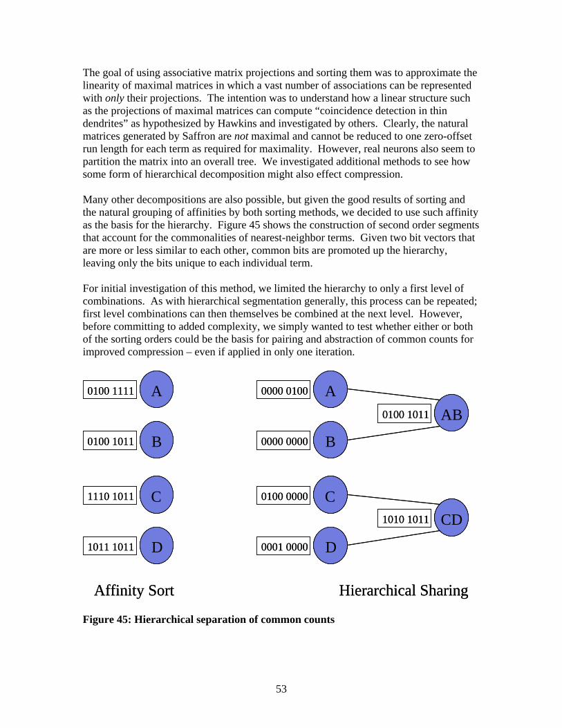
53

The goal of using associative matrix projections and sorting them was to approximate the linearity of maximal matrices in which a vast number of associations can be represented with only their projections. The intention was to understand how a linear structure such as the projections of maximal matrices can compute “coincidence detection in thin dendrites” as hypothesized by Hawkins and investigated by others. Clearly, the natural matrices generated by Saffron are not maximal and cannot be reduced to one zero-offset run length for each term as required for maximality. However, real neurons also seem to partition the matrix into an overall tree. We investigated additional methods to see how some form of hierarchical decomposition might also effect compression. Many other decompositions are also possible, but given the good results of sorting and the natural grouping of affinities by both sorting methods, we decided to use such affinity as the basis for the hierarchy. Figure 45 shows the construction of second order segments that account for the commonalities of nearest-neighbor terms. Given two bit vectors that are more or less similar to each other, common bits are promoted up the hierarchy, leaving only the bits unique to each individual term. For initial investigation of this method, we limited the hierarchy to only a first level of combinations. As with hierarchical segmentation generally, this process can be repeated; first level combinations can then themselves be combined at the next level. However, before committing to added complexity, we simply wanted to test whether either or both of the sorting orders could be the basis for pairing and abstraction of common counts for improved compression – even if applied in only one iteration.

Affinity Sort

C

D

1110 1011

1011 1011

A

B

0100 1111

0100 1011

C

D

0100 0000

0001 0000

A

B

0000 0100

0000 0000

AB0100 1011

CD1010 1011

Hierarchical SharingAffinity Sort

C

D

1110 1011

1011 1011

A

B

0100 1111

0100 1011

C

D

0100 0000

0001 0000

A

B

0000 0100

0000 0000

AB0100 1011

CD1010 1011

Hierarchical Sharing Figure 45: Hierarchical separation of common counts

54

Figures 46 and 47 show the compression results of hierarchical sharing based on both strength sorting and affinity sorting.

Figure 46: Strength sorting and hierarchical grouping

Figure 47: Affinity sorting and hierarchical grouping

55

In both cases of strength sorting and affinity sorting, hierarchical sharing across nearest neighbors improved the compression over sorting along. The trend lines for all 4 cases are shown in Figure 48.

Figure 48: Comparison of all sorting (solid line) and sharing (dotted line) cases Affinity sorting appears better than strength sorting and hierarchical sharing appears to improve both, respectively. The hierarchical sharing method also continues to fulfill the requirements of a lossless and incremental memory. For example, the individual term segments remain as the places where new associations are observed. The hierarchy is irrelevant to how new contexts are written into the memory. The consolidation of shared counts can occur at any time other than the time that they are observed. This is resonant with the idea that associative changes might be rapid, but that consolidation can take more time and occur later (after learning per se, perhaps as a function of sleep) .

4.5 Larger Scale However, our results are extremely tentative because of the restricted range of Small Matrix sizes that were measured. As a last effort of this work, both forms of sorting and hierarchical sharing were applied to a sample of larger Small Matrices. While the method used for these experiments is still extreme inefficient (reading and resorting the matrices from disk) and we would like to know more about even larger matrices, this final experiment sampled matrices up to 2500 attributes. Figure 49 shows the continuation of the compression effects. Affinity sorting continued to be the better method, and hierarchical sharing continues its additional improvement. Therefore, we have selected only affinity sorting for going forward and show only these

56

results. (Matrices smaller than 300 were excluded in order to determine the later sections of the scaling curve.)

500 750 1000 1250 1500 1750 2000

0.4

0.5

0.6

0.7

0.8

Figure 49: Larger sampling of affinity sorting (red) and sharing (green) methods The regression curves are now polynomial. However, given the degrees of freedom in polynomials and the limited sample size at the larger attribute numbers, it is unclear whether the tail of the curve is asymptote or reversing. It is entirely possible that the compression effects will become even greater as the matrices grow beyond 2500 attributes and the matrices become sparser, but this is extremely uncertain without more data. Subsequent work using hardware acceleration to more efficiently explore much larger dimensions will better determine whether this trend persists or not. If so, then these results could have more impact on the overall scalability of SaffronOne. For instance, empirical results suggest that transition to a Large Matrix should occur at 10K attributes. If resorting and sharing has significant compression effects at the Small Matrix approaches 10K, then this switch point may be pushed out to 20K-40K attributes perhaps. Further research and develop of the hierarchical sharing method is also likely to improve the results. For instance, as in a full tree, the method can be recursively applied to the hierarchical groupings adding (perhaps) another 10-20% or greater size reduction. To do this, a cost/benefit decision method should also be included. For example, even if some bits can be shared in the hierarchy it might not be more efficient to do so for specific branch points, depending on the case. More like real neurons that are tree-like but not complete trees, it is likely that the efficacy of sharing will halt the recursion at various

57

points, creating a sparser tree. This cost/benefit decision rule is not yet applied to even the first order sharing; therefore, the compression benefits now cited are likely to be an underestimate. The shared hierarchy was formed and then measured in total, whether more efficient or not for each decision point. Future results should be even better. Sorting and sharing seem profitable to continue and improve. Saffron is a memory-intensive application and any reduction of footprint is beneficial. Not only do such compressions decrease the precious cache requirements for resident matrices, it also decreases the overall persistent requirement by half. Moreover, smaller matrices will also improve time performance in both allowing more matrices in a given cache and in better transfer of matrices through the I/O bottleneck. As a general rule, Saffron’s concerns about compression have benefited the more critical issues of response time rather than footprint per se. Such accomplishments will be pursued in both our software product and in subsequent hardware efforts.

4.6 Hardware Considerations

4.6.1 Neuromorphic Chips As evidenced in the latest issue of Scientific American and the article entitled, “Neuormorphic Microchips” (Boahen, 2005), research on neural hardware is active and popular. This article also discusses self-organization by the swapping of “softwires”. As seen in Figure 50, the map from external input in ganglion cells is modified by activity. Given a random initial wiring, the wiring to tectal cells moves closer to its source of stimulation so that internal maps come closer to the external order.

Figure 50: Self-organization of receptor map based on swapping of “softwires”

58

However, such self-organization is more typical of receptive fields and is based on gradual, developmental processes. This is different from our sorting in both method and purpose. This process is slow and highly iterative. Self-organizing maps are very likely true of real neural development, but it is a slow developmental process, not a fast memory consolidation. We prefer a more instant sorting function based on projections, but such general principles of self-organization are very similar. Other neuromorphic research such as in hardware-based “softwire” will be informative to future implementations of the sorting methods. The existence and speed of neuromorphic change in real neurons is still controversial. The classic doctrine is that such self-organization occurs during development but not in adulthood. Learning might take place as a matter of local change in synaptic strength, but synaptic movement, new synapse formation, and dendritic branching changes were thought impossible. Recent evidence suggests that neuromorphic changes also occur in the adult. For instance, new synapses have been observed following LTP by minutes to hours (Lamprecht and LeDoux, 2004). This is relevant to the scheduling of memory consolidation. The associative counts are updated instantly, but sorting can be a delayed as a secondary process of consolidation. For instance, a Small Matrix can reside in cache memory and rapidly observe a number of new contexts. When saved to persistent storage at some arbitrary later time, this is when it can be resorted as a matter of consolidation. The hesitancy to believe in adult neuromorphics has been due to lack of empirical evidence, which has been due to the lack of neuranatomical techniques to generate such evidence. However, as shown in Figure 51, new microscopic methods are allowing neuroscientists to see and measure such changes (Lamprecht and LeDoux, 2004).

Figure 51: LTP induced spine growth over minutes and hours following learning If synaptic “movement” is a matter of such rewiring, then LTP changes in associative counts can be immediate, while such consolidations are then induced but made later. Such consolidation is not required to initially store the new memories, but only to better organize them.

59

4.6.2 Parallel sorting There is also a large body of work on hardware-based parallel sorting algorithms. Even inefficient sorts like Bubble-sort are more reasonable when made parallel. On the other hand, specific parallel algorithms such as a Batcher’s Bitonic sort are extremely efficient in hardware. While the basic algorithm is well known, specific implementations in FPGA is an active area of research for considerations of concurrent and block-wise memory access (Layer and Pfleiderer, 2004). VHDL implementation of a sort method was explored early in this project but was then considered as best left to future implementations. These initial efforts in message-passing in a linear hardware structure for maximal matrices have been described in interim reports, but the implementation of affinity sorting is now the priority concern going forward. As discussed below, message-passing methods were explored, but it was very unclear whether this is advisable for hardware realization. The decision depends on which sorting method is found to have better compression across scale, which is yet to be finally determined. For instance, affinity sorting is a variant of a bubble sort, which could be implemented as message passing for localized swapping. However, if strength sorting were found better, then this is a standard descending stable sort of projection strength. In this case, the best general purpose hardware sort, such as bitonic sort, would be the best decision in this case – not a modified bubble sort. Given the more complex sort and merge components of a bitonic sort, message passing would not be suggested. However, now that affinity sorting seems to be better than strength sorting, the Figure 52 outlines how the translation table needs to be extended.

Prior-NextProjections

CurrentIndex

InternalAttribute

Prior-NextProjections

CurrentIndex

InternalAttribute

Prior-NextProjections

CurrentIndex

InternalAttribute

Prior-NextProjections

CurrentIndex

InternalAttribute

Prior-NextProjections

CurrentIndex

InternalAttribute

Prior-NextProjections

CurrentIndex

InternalAttribute

Lookup Attribute-Index

Observe New Projections

SortSwap

SortSwap

Figure 52: Small Matrix translation table for affinity-based sorting Much like softwire swapping above, the table must hold the current translation order as well as the prior-next projections for the given order. As new observations are loaded

60

into the matrix itself, the prior-next projections must also observe and change along with the matrix itself. Such projection changes can be easily computed from the context; projections should NOT be recomputed by scanning over the matrix per se. These projections can then be swapped using a modified bubble-sort as described above. Once the matrix is also modified to the new sort order, then the new order can be used as the current order. More like neural self-organization, the sorting of the translation tables is really only sort-maintenance. The expected design is to compute the next sort order to a Small Matrix while it is in cache and then stream the matrix content from the cache to persistence in the new order. When the matrix is fetched again, it will be in the new order. Therefore, the matrices will tend to need only partial resorting each time, since the majority of the matrix will be in order and is altered only by the effects on count changes for a new observation. As matrices grow larger and gain more experience, the relative power of each observation to change the sort order will be continually reduced. The sorting order will self-organize and stabilize over the long-term, and even when they grow beyond the bounds of a single block in cache, the history of the matrix sorting at smaller size and the limit of sorting even within each block should be sufficient. Local message passing and swapping is likely to be very efficient. This approach can also support an anytime algorithm; depending on other resource demands, sorting can be arbitrarily delayed. It can also be partial. Any swapping moves the structure to a better state without requiring that the entire sort is completed. Even if some sorting is accomplished at one phase, the matrix can be further consolidated at some later time – without effect to the perfect content of the memory itself. At the time of this writing, a combined method of strength and affinity sorting is unknown but is suggested for further thought. Proximal (near the base soma) synapses are thought to be stronger than those that are distal (away from the soma). Affinity between synapses is also widely thought to occur in the organization of dendrites as illustrated in Figure 53.

Strong Base

Affinity Groups

Figure 53: Theory of Neural Structure based on some combination of sortings It is unclear how the sort methods and hierarchical groups map to a dendritic tree structure for coincidence detection. But from the single matrix perspective, strong attributes should clearly be at the matrix “bottom” for improved run lengths while

61

affinities should be gathered together for “long and thin” matrix organization along the diagonal. Furthermore, while explicit sorting of projections has been explored here, activity-based self-organization might cause such re-ordering as demonstrated by neuromorphic softwires. In other words, as contexts are observed, the synapses might move together in response to each context rather than as an overall sort. But this is all unclear at this time.

5 Accomplishments and Lessons

5.1 Project Results This work evolved through various accomplishments and setbacks which shifted priorities along the way. Through these changes, decisions were made to pursue those avenues that would continue to drive toward eventual hardware implementation and be most profitable to further understanding of possible neural algorithms that would also be part of future hardware. Some work was halted because it was inappropriate for such redirections (such as not placing Cognitive Constructs in VHDL) or because it became too uncertain without more fundamental understanding (not pursuing message passing in VHDL until sorting was better understood). However, the two major initiatives each produced positive outcomes that will be profitable for continued work:

• SaffronOne in VHDL. Saffron is a software company. This work was the first step in moving its products to hardware (at least the hot spot core) and providing an appliance model for enterprise scale. Saffron personnel are not capable of synthesis and implementation, but as a first step in moving from software to hardware, our core methods are now explicitly documented and also described in VHDL behavioral models. We believe that subsequent work with hardware experts will re-design, but our work is at least a communication vehicle to quicken such implementation. Rather than starting from scratch, all of the core functions – except for bit-plane growth – are described. Even basic functions for segment offsets, space filling curves, and such are clearly described for transfer to subsequent experts. Both Large Matrix and Small Matrix algorithms were described. Also, two designs of more naive implementations were described for boot-strapping and comparing them to the more complex structures.

• Additional compression. The Holy Grail of understanding dynamical dendritic structure and coincidence detection was not achieved, but very practical progress was made as a by-product of continuing to pursue Saffron’s ideas. The perfection of compressing maximal matrices into a linear form did not progress to a more general case. Several hypotheses about how to pursue these ideas were generated, and the exploration of projection-based sorting resulted as a practical result. Strength sorting and affinity sorting were both explored, but some future combination might still be most promising. Although of long-time interest to Saffron, renewed research into large matrix sorting found new ideas in the literature about nearest neighbor definitions and the equivalence of matrix sorting to the TSP. Projection sorting emerged as a practical answer. Moreover, once sorting was established, the idea of hierarchical sharing of affinity neighbors was also found to be additionally effective in further compression. Early work on message passing hardware was halted until such results were known (bitonic

62

hardware sorting would have been more effective for strength sorting), but subsequent implementations of the core in hardware should also include these sort methods, most likely in a message-passing, modified bubble sort.

Continuation of this work will pursue implementation of the SaffronOne Small Matrix in VHDL along with the addition of sorting its translation table. Saffron also intends to investigate patent protection of the new compression methods. Elements of matrix projection and sorting have been claimed in past filings, but the added methods might also have merit as a new invention due to this work.

5.2 Distributed Product Design During the course of this work, Saffron was also re-developing its products toward a distributed system design. Our thinking about the hardware interface also affected our thinking about distributed product design. Two principle design points are now common to the VHDL interface and SaffronOne’s service interface:

• Index interface. Earlier versions of the SaffronOne interface were intended for single process functions, such as to support OEM applications. The application would define its context in its own semantics of attribute-value and call SaffronOne for all translations and other processing. However, in separating concerns into a distributed service system, most of the surround support functions such as translating external attributes into internal attributes have been separated from the core memory. Now as a separate service process, SaffronOne assume that all context descriptions are referenced by the translated indices. As we also investigate hardware partners for subsequent work, this design point seemed to be shared with other distributed platforms.

• Count service. SaffronOne’s single process services also included a number of various inferencing options. For instance, SaffronOne would use entropy-based or Bayesian-like computations across the matrix counts. The product’s internal object architecture separated the counting from the inferencing, but when moving to a distributed system, this object separation became a process separation. The primary concern of SaffronOne is now to update, serve, and accumulate raw counts. These raw counts, in addition to the individual matrix counts, as also defined by the primate measures of experience (sum or associative counts) and novelty (absence of associative counts). As decided in this project to port SaffronOne to VHDL, other inferencing options are so various and dependent on the application that they were not also described in VHDL. As in the current product and as the expected “hot spot” for hardware replacement, SaffronOne is now focused on efficient multi-agent, associative matrix management.

The distribution of service functions and such interfaces for the SaffronOne core in the software product also align it for subsequent re-implementation and replacement with hardware.

5.3 Hardware Inexperience Finally, we learned that the difficulties of moving from a software basis to a hardware basis were harder than expected. Saffron is a software product company and we

63

underestimated the process and tool experience and costs in porting to hardware. Because this work was just the first step with very high risks, it was inappropriate to staff Saffron with hardware expertise for a short term and uncertain future. We had some VHDL experience to draw on – and did make good progress – but we also now see that outsourcing and partnership with hardware expertise will be faster and more productive. On the other hand, the port to VHDL and the increased understanding of the neural device have established some strong assets to continue this work and realize an associative memory building block. Based on the results of this work and other continuing demands on Saffron’s business, we now have even more motivation to implement SaffronOne in hardware and make it available for cognitive system applications at extreme scale. As discussed in Future Directions, increased scalability is the highest current business priority. We intend to outsource/partner for greater hardware experience. We also intend to include the SaffronOne core developer who is an EE by historical training. As we pursue this business and grow the company at large, additional hardware experience is likely to be a factor even if only for coordination with partners, but we now better understand the difficulties and issues for success.

5.4 Application Scope Saffron has always considered the two options: scaling up to massive data problems and scaling down to embedded systems. Hardware forms of associative memory will be required for both. For example, hardware acceleration of algorithms will used to increase scale while hardware embedding will used for miniaturization. Saffron’s initial considerations were focused only on scaling down to embedded systems as a new, future business. Saffron’s current business is focused on scaling up to massive databases and memory bases. As the project requirements unfolded, the shift was toward AFRL’s and Saffron’s needs for hardware acceleration in Information Management. But even within this scope, we began to understand different requirements between most current approaches and what Saffron is trying to do. The development of the building block in VHDL, for now, is independent of these application drivers, but in moving forward to implementation and as a matter of different Cognitive Constructs, we now understand the following differences:

• Microchip embedding. Many future applications of associative will require an on-board or in-device memory chip. These will be fixed-capacity system and the design of the building block and surround cognitive constructs will be hardwired into the design. The current VHDL is close to this design in assuming that an entire memory will “fit” within dedicated FPGAs, for example. This is neurologically realistic; neurons are devices that both process and store memories that are always “resident” in this sense. There is no separation of process and memory and is optimized for real-time, constant use by the specific application.

• Massive ingestion. Within the more general purpose scope of Information Management, hardware acceleration is needed more for the massive throughput of data. Rather than a small device model, specialized hardware is used within large, high performance systems. However, all current approaches have a traditional assumption in trying to accelerate “ingestion”. Most cognitive algorithms and

64

supporting methods assume fixed runtime models. For instance, entity extractors, decision tree and other classifiers, latent semantic indexing, concept mapping, and virtually all other vendors and research initiatives use the phrase “ingestion rate” to describe how fast a fixed model can process an incoming stream of data. Like rules, decision trees, latent semantics, neural classifiers, entity extractors, and more, these models are reductionistic. As such, these models tend to be reduces to a size and function in which they are complete resident in a large “sea of gates” or cache memory. The common idea is that a fixed model is resident and can rapidly apply its model to the incoming stream, such as to quickly extract concepts or classify documents, for example.

• Massive assimilation. These other approaches can only “ingest” at high rates because they are not incremental and lossless models like Saffron. For example, decision trees, most neural networks, latent semantic indexing are all built offline in slow, parametric batch-mode knowledge engineering processes. They are totally incapable of building and modifying their models as also a matter of ingestion. This is the way the brain works. Unlike abstracted, reductionistic models that cannot by their nature be truly incremental for on-the-fly learning, Saffron observes and modifies its models as a process of assimilation. Like real neural learning, new data is embedded into the existing knowledge representation, which involved the more complicated issues of growing and managing the representation. Not only this, Saffron manages millions of such models, which cannot possibly all reside in cache at the same time.

These realizations became clearer as this project considered the various Cognitive Constructs required for different Information Management applications and how the project managed its resources for future practical success. The Publish-Subscribe architecture of the Air Force Research Lab’s Joint Battlespace Infosphere (www.rl.af.mil/programs/jbi) is one example. The issue is in whether the high-event rates are driven to new observations (writes) or imaginations (reads). In such systems, the resident model must represent user subscriptions and serve as a router of new publications to such subscriptions. As such, observation events are defined by user subscription requests. These are low volume. High performance is required to handle the high rate of publication. As described in Future Directions, Saffron is most stressed by real-time-modeling of the new data. In other words, whether through a pub-sub architecture or in any other case in which massive data needs to be modeled and indexed, the focus needs to be on the speed of assimilation to model the publications, not the subscriptions. Saffron does also model users and user events, but these models are used to refine query intentions. Query rates are also much lower than source publication events; therefore, the fetching, updating, and query of user models is also not as taxing as source modeling. For continued interests of JBI, this means that Saffron’s massive assimilation and memory modeling should be applied to it Query Service. Saffron would subscribe to all new content entering JBI in order to provide a knowledge-level memory base of all people, places, and things in the total repository.

65

Saffron’s architecture for massive source modeling makes such associative memories very memory-intensive and storage-intensive, not CPU intensive. In addition, the I/O bottleneck of Von Neumann architectures is the overriding issue, which is why compression and partitioning are so important. Saffron memories are universal and can also be applied to large but single model classification (hetero-associative) and latent semantic indexing (auto-associative), but because such smaller fixed-models might be adequate, such applications are not as discriminating of Saffron. Context-dependent, incremental learning at massive scale is much harder and more valuable, but these rates and dynamics push the need to very flexible hardware acceleration, including issues of mass storage and high performance I/O.

5.5 Theory Advancement It is hard to describe conceptual progress when the final answers are not yet clear. For instance, we cannot yet say exactly how neurons compute coincidence detection in thin dendrites. While maximality is intriguing and sorting and hierarchy are better are now better understood, we still cannot report a complete, coherent theory. However, we feel that this work has moved our conceptions closer to a true understanding. Aside from the bit-planing, segmentation, sorting and hierarchy that have been discussed as major elements of the solution, a number of smaller but significant points have also become clearer over the course of this work:

• Maximality is not required to still pursue the benefits of sorting. While maximal matrices are perfectly compressed into linear projections, this extreme is not required for progress. Projections of a maximal matrix are also now seen as zero-offset run lengths. We also considered schemes for message-passing reads of run lengths with non-zero starts and how perfect run length encoding might work. But when nothing was clear and successful, the benefits of sorting toward better run length encoding remained profitable. Maximal projections still provide the best example of representing a large number of associations and reading the matrix as a form of coincidence detection using only the sort order of this “thin” linear structure. Sorting creates fewer run lengths in general, but there is still a gap in understanding this ideal structure for thin dendrites and the complexities of real associative matrices.

• Projection sorting is commutative across a complete matrix. The VHDL design was limited to a single “existence” plane. Also, many if not most examples in Advanced Explorations show single bit vector examples. However, the methods and results for sorting and sharing were based on complete, associative counts. For example, the strength and affinity projections were defined not just as the number of associative bits; they were defined as the sum of associative strengths. In earlier implementations, Saffron tried to sort each bit plane; however, the translation tables for each bit-plane can be come more expensive than the savings made by translation table sorting. However, the translation table is now at the level of the entire Small Matrix. It is also a “sunk” cost in that each Small Matrix needs one. In the case, the sort order of the single table is “free”. We discovered as a course of this work that projections based on total association counts across bit-planes still effects the compression of each bit-plane. In other words, the sum of bit-plane projections has a commutative effect

66

in that the sort of the total sums has the equivalent effect of sorting each plane and summing the separate effects. Whereas, sorting of each plane had less practical value due to the cost, the current method is more “free” and of practical value.

As described above, there are still many uncertainties in moving these discoveries into product. This AFRL support was a rare opportunity to pursue some ideas that we believe will eventually lead to a breakthrough general theory, although it is now time again to move these results into practice. As described below, the project has lead to much greater clarity with good results for moving forward.

6 Future Directions

6.1 Appliance Model There are many past failures of AI and NN hardware efforts. For example special LISP processors and neural network accelerators have been developed in the past but without much (if any) market success. There could have been many reasons for these past failure, including the fact that the underlying technologies were to young and ineffective to support a mass market. For example, AI itself has had limited success – hardware or software. This is less true of neural networks, but even here, the availability of cheap general purpose computing never allowed special purpose accelerators to have much benefit/cost, except in the most dedicated, embedded applications. This argument remains with force: A hardware solution must significantly outperform a software solution on general purpose hardware in order to compete. But the software world is also changing and other costs of installation and maintenance are changing the equation, especially for large-scale enterprise solutions. The costs of software installation, configuration, and maintenance are driving many applications to an “appliance” model. This model provides the customer with a complete solution in a hardware box, which is then simply be inserted into a local network. Entire, enterprise-scale solutions can be pre-configured by the provider for simple installation to the customer. Other industry dynamics are also forcing the need for hardware-based appliances. The growth and distribution of data and documents is unprecedented. For example, databases are so large that many data mining techniques are virtually impossible without acceleration. Companies such as Teradata and Netezza are addressing the need for “data appliances” to make even basic queries of massive data at scale. Even for basic SQL queries that find non-obvious relationships across a number of databases, companies like Seisint (now Lexis-Nexis) are largely based on a parallel, distributed query platform. In the area of unstructured indexing and search, at the scale of the Web, Google and other search engines require massive operation centers and our now selling “search appliances” for corporate enterprises to manage their own internal documents.

67

Saffron software solutions have also outperformed one competitor, Non-obvious Relationship Awareness (NORA, now owned by IBM), in accuracy (only 2% success compared to Saffron’s 80% success) on a most difficult intelligence problem. Now called IBM DB2 Identity Resolution, the hardware costs are 10X software costs. Increased Saffron hardware performance can also compete on total price/performance as well as the proven difference in accuracy. Saffron is in some sense another form of database, although a memory base. We provide a search and index system for massive amounts of structured and/or unstructured information, but what is more difficult, we do this at the level of real-time knowledge based on real-time associative memories. Saffron is associative, not relational, which opens up a number of new and more powerful cognitive abilities. Saffron is also planning to re-enter the commercial market and has plans to approach the major search engine companies within this year, but current government customers are now the most demanding. The need for continued scaling, which will require hardware acceleration, is the most pressing issue for many current efforts for the government:

• Data disambiguation. Saffron has proven its unique ability to solve on of the most difficult problems across the intelligence community. Working in the Research and Development Experimental Center (RDEC) for agencies such as the CIA and DIA, Saffron has developed an analogy-based method for detecting aliases and other ambiguities, not just within one database, but across different databases across different agencies. As just described, the nearest competitor failed this test on real foreign intelligence data (2% accuracy) while Saffron was recently measured at 80% accuracy. A small but multi-server system has been proven to join two databases of over 100K-200K entities each, but this is just the tip of the iceberg. Many, many more databases are intended for future work, the total number of entities that will need modeling needs another order of magnitude (or two) to cover the number and size of relational and transactional data that should be ideally considered.

• Open source intelligence. Saffron has recently started a new effort under the Topsail Project (classified owning agency, but administered through AFRL) in partnership with Factiva, a Dow Jones and Reuters Company. Stress testing of Saffron is a first order of investigation. Saffron will install itself within Factiva’s operations center, which receives 100K-200K news documents/day. This is within Saffron’s current capability, but the very long-term performance of a year or more is unknown. Factiva also has 30 years of open source news that should also ideally be observed by Saffron. This volume is likely unreasonable without hardware acceleration to assimilate such a large backlog to support OSINT.

• Deep Web mining. Although nothing is in contract or even qualified, Saffron was recently approached by IBM to work on its WebFountain solution within DIA. In case, the rates will be millions of documents/day.

Embedded applications remain as an additional future of associative memory hardware, but toward Saffron’s nearer-term business interests, we intend to provide our current enterprise software solutions within such an appliance model and are thankful to AFRL for the past and future support.

68

6.2 SBIR Continuation Thanks again to AFRL, Saffron has been awarded a Phase I award for continued research and business innovation in Cognitive Hardware. While Saffron personnel were able to describe the core memory representation and functions in VHDL behavioral models for this current work, implementation and synthesis will be outsourced to hardware experts for the SBIR continuation. More than this, expertise in leading edge FPGA application is required to configure the system at large. For instance, because Saffron is I/O intensive, a SaffronOne microprocessor for the core computations is only part of the required solution. How such an FPGA micro-processor interacts with cache memory, distributed communication bandwidth, and massive memory persistence mechanisms must also be defined for a complete solution. Toward the “business” of an SBIR, Saffron intends to prototype its Saffron Enterprise Platform as a software/hardware mix for its most demanding customers. Toward the “research” of an SBIR, Saffron will partner with a research institution for properly exploring novel hardware solutions for such a platform. Saffron intends to collaborate with John Lockwood from Washington University in St Louis. This collaboration will leverage other existing work by Saffron and by WUStL that are both currently under SAIC testing and integration at RDEC (under classified DoD ownership). The effort now has all 15 intelligence agencies and a growing number of military commands as its customers. Both Saffron and WUStL have provided outstanding, independent results to date:

• Saffron Technology. For example, Saffron uniquely solution to the alias detection and multi-database disambiguation problem has already been described. SaffronWeb for Discovery and Sharing is also being evaluated as yet another core application for the center. In general, Saffron is seen in RDEC as the breakthrough technology for many of the hardest problems – at scale. On the other hand, while Saffron’s software solution has scaled to millions of attributes per associative matrix and millions of such matrixes for tracking various people, places, and things, the demands of RDEC customers and the future requirements of the intelligence community are driving the need for even further scale, best provided by hardware.

• Washington University. In compliment, WU St Louis is also a key component of RDEC toward automating the “front end” content processing of very high throughput. The goal is to apply advanced cognitive algorithms to Internet data rates. As shown in Figure 54, stacks of WUStL’s Field Programmable Port Extender (FPX) implement various processing methods, from simple parsing to high level semantics at very high rates. For example, WUStL has ported Latent Semantic Indexing (LSI) to such hardware and is categorizing 30,000 documents/second.

Beyond the FPGA-based core processing, this platform is also ideal for software/hardware mixing. The FPX interfaces support IP protocols for TCP or UDP communication to other network subsystems, which might be other FPXs or other software application of persistence subsystems. Each of the hardware modules is

69

equipped with 2 banks of pipelined SRAM and 2 banks of SDRAM. Each can do up to four memory operations per hardware clock cycle. Up to 1 Gigabyte of memory can be loaded onto each module (512MBytes on each of 2 SDRAMs, and 2MBytes on each SRAM). The FPGA is a Xilinx Virtex 2000E (about 2M gates of logic).

Figure 54: FPX Configuration for deep context processing at Internet rates The SBIR plan is to complete the work begun here and implement the VHDL within an FPX module. Many elements of the Saffron and WUStL architectures are similar. For instance, both systems include additional infrastructure to parse the ingestion flows, parse documents, and identify semantic words by index through an atom table. Both are distributed, multi-processor systems in which the core algorithms (whether Saffron or LSI) receive IP packets with index-based description vectors of the original content. Saffron and WUStL both have installations managed by SAIC within RDEC. The plan is to install SaffronWeb on the WUStL software/hardware platform and then replace the SaffronOne software servers with FPX-based equivalents using the same network-based, index-based interface from one to the other. It is critically important to also understand that this work must address more than just the FPGA implementation of the Saffron VHDL as described above. As already mentioned, Saffron is not a static-model like LSI and requires more than in-memory residence of such a model. Two issues must be further addressed specifically for Saffron’s approach to associative memories at massive scale:

• Dynamic assimilation. Unlike LSI and almost all other machine learning approaches, Saffron allows for incremental learning. Rather than training phases that build a model and then load a static version of the model for runtime use, Saffron is a memory that can be constantly updated even during its use. Such

OC-192 .. OC-768(10-40 Gbps)

All trafficpassing through

network backbone

OC-48(2.5 Gbps)

…

Network Switch

Content Scannerin reconfigurable

hardware

OC-48(2.5 Gbps)

OC-192 .. OC-768(10-40 Gbps)

All trafficpassing through

network backbone

OC-48(2.5 Gbps)

…

Network Switch

Content Scannerin reconfigurable

hardware

OC-48(2.5 Gbps)

Field-programmable Port Extender (FPX)

Process TCP/IP traffic flows Prune

Stem

Ingest Content Rapidly

has is wa

informati -> presiden -> presi

Cognitive Methods

Count and score

Display and Analyze

Process TCP/IP traffic flows Prune

Stem

Ingest Content Rapidly

has is wahas is wa

informati -> presiden -> presi

Count and score

Display and Analyze

70

dynamics push the meaning of “flexible” hardware. We are very uncertain of how the VHDL tree growth and other dynamics will survive synthesis and implementation. The current VHDL design assumes more of an embedded system design in which the Saffron structures are entirely within the FPGA. Instead, it might be more reasonable to implement a micro-processor version of the methods in which the structure itself is manipulated within the memory cache. In any case, this is left to the hardware development experience of WUStL, which has implemented many other algorithms and complex data structures in the past.

• Massive storage block device. The WUStL installation at RDEC already includes a large scale Storage Area Network (SAN). Saffron is also investigating the use of a SAN to improve its own scaling, software or hardware. Saffron is planning a re-design of its persistence layer in order to more directly work with block-devices. Currently, Saffron stores are memories in any JDBC-compliant database. There are many benefits to commercial database persistence, but it is also wasteful to Saffron’s core persistence needs. The blocks described about are merely stored as “blobs” in the database. The block addressing is simple and there is nothing relation in the content that requires the relational overhead. As such, Saffron is moving to remove the database requirement and more directly control the I/O as its own block device and we are exploring the block device interfaces provided by SAN vendors. A “raw” block device interface will be used to support the persistence of SaffronOne servers, whether in hardware or software. Saffron will define this block design implementation in coordination with WUStL for common use.

Both of these elements seem within the capability of WUStL personnel and the FPX platform. Saffron will provide the current VHDL description to bootstrap the new design and work together to define the block device storage strategy. WuStL has implemented many other algorithms in hardware de novo (such as LSI from SAIC and associative methods from Fair Isaac); therefore, Saffron’s VHDL descriptions should accelerate their process. A key to success will be to focus the hardware implementation on a specific “hot spot” function. The VHDL behaviors of the current work include both the observe (write) function as well as basic imagine (read) functions. In actuality, Saffron’s distributed system design separates the observe and imagine functions into two, separately dedicated processes as shown in Figure 55. We intend to focus the hardware implementation on the following elements:

• Observation processor. Both observe and imagine functions are desirable, but we will focus on accelerating the observation rate as the bigger bottleneck.

• Affinity sorting. The sorting methods will also be added to the implementation in order to further compress the memories, such as when moving from cache to storage.

• Block storage. I/O is the primary bottleneck to current performance. Block device interfaces and other relevant architectural issues will be addressed to overcome this bottleneck.

71

HardwareObserve

Storage Network

HardwareSort

SoftwareImagine

SoftwareConstructs

HardwareObserve

Storage Network

HardwareSort

SoftwareImagine

SoftwareConstructs

Figure 55: Distributed hardware/software processors across by massive storage Of course, as one bottleneck is removed, others such as communication bandwidth will become the next limiting factor. Contractually, the first task of the SBIR is to research an appropriate platform, which must also be with an academic institution. Of options are also available, but the WUStL FPX platform and personnel seem ideal. For one, this choice will leverage the common SAIC arrangements within RDEC, which is very metrics oriented and provides a source of massive data. Second, John Lockwood and the FPX platform are also associated with a venture company called Global Velocity. The outsourcing of SBIR work can enjoy the rates and research benefits of an academic institution while also already having a commercial organization for subsequent platform availability as a partner. Otherwise, one of the first tasks will be to develop a test plan. In order to better plan the implementation scope, the volumes and type of data will be defined along with the expected goals of the system. For example, the desired (sustainable) assimilation rate should be determined up front in order to then design the system for such goals. The test plan and metrics will focus on:

• Observation speed. Software and hardware modules should conform to the same interface and be plug-and-play. This will allow comparison of assimilation rates between software and hardware. This will be described functionally as documents/second and/or structurally as associations/second. Desired and actual speed up will be reported.

• Persistence size. Increasing the observation rate to new levels will also drive the storage requirements to new levels. Increased storage costs must also be

72

accounted. This will drive the need for sorting-based consolidation, which should improve these storage costs. Small matrices will also improve bandwidth and likely improve overall observation speed as a side effect. The inclusion of sorting-based consolidation will be considered as an option in order to measure and report such differential effects.

The goal accomplishment of this work is to demonstrate a prototype software-hardware appliance model of Saffron’s product that would address the high performance demands of Saffron’s current customers and the interests of JBI.

6.3 Quantum Neurons Several neural network algorithms, including associative memories, have been proposed in as theoretical quantum algorithms. For instance, a form of associative memory has been derived from Grover’s algorithm for quantum search (Ventura and Martinez, 1998). This model has even been simulated against standard machine learning databases and shows exponential memory capacity. For example, one test with 200 patterns was learned by only 7 quantum “neurons”. Another body of research also suggests that neurons and brains are quantum computers (Hameroff, 1987). As in Figure 56, these quantum effects are believed to exist in the microtubules within dendrites. In the same way that dendrite segments are thin, linear structures, the interiors of dendrites are filled with long, thin microtubules. While traditional thinking held these as merely skeletal and supportive of neural structure, there is also speculation that the microtubules are fundamental to neural computation. The tubules protein elements might provide an electron switch, and since this speculation also holds that the interior of the microtubules can provide the isolation required for long-range quantum coherence.

Figure 56: Microtubule with electron switching and electro-isolated interior

73

On the other hand, the theoretical speculations about quantum algorithms also have a neural counter-argument. Even if neurons do use quantum effects to speed computation, there is a big difference between the vast number of atoms and complex molecules used by real neurons and the single-atom power that is assumed by quantum computing. For example, the quantum dream is that a 64bit quantum computer can be implemented by only 64 atoms. Although all such things are possible, we suggest that this position for hardware intelligence is equivalent to the hubris of AI during its early years. AI assumed that computers would surpass human cognitive ability within a decade of its founding in 1957. Its philosophies rejected the idea that actual brains were fair superior and that the “wetware” that supported cognitive functioning might hold the keys to improved computer design. We suggest that real neurons might indeed use quantum effects but that quantum computing has limits – more to the scale of “wetware” abilities already found by neural evolution. In fact, separate from any consideration of quantum neurons, some experts in general quantum computation warn of many uncertainties. For example, the exact mechanisms of quantum effects and the nature of quantum coherence are still unknown (Brooks, 1999). The limits of coherence and the ability for individual atoms to entangle with each other might hamper the reality of building a 64bit computer with only 64 bits. Quantum entanglements and coherence might have limits even if real neural systems use quantum effects within these limits. On the other hand, if individual atoms and nanostructures do have quantum limits, then the partitioning and ordering explored here and seen in neuromorphic structures might also be relevant. Neural architectures will likely continue for many decades to be the inspiration for cognitive architectures, whether using quantum effects of not.

74

7 References Aha,David W. Editorial. Artificial Intelligence Review, 11(1-5):1-6, 1997. (Special Issue on Lazy Learning). Boahen, Kwabena. Neuromorphic Microchips. Scientific American, May, 2005 Brooks, Michael, editor. Quantum Computing and Communications. Springer: New york, 1999. Goharian, N., A. Jain, Q. Sun, Comparative Analysis of Sparse Matrix Algorithms for Information Retrieval. Journal of Systemics, Cybernetics and Informatics, 2003. Hameroff, Stuart R. Ultimate Computing. North-Holland: New York, 1987. Hassoun, Mohamad H., editor. Associative Neural Memories: Theory and Implementation. Oxford University: New York, 1993. Hausser, Michael, and Bartlett Mel. Dendrites: Bug or Feature? Current Opinion in Neurobiology, 13:372–383, 2003. Hawkins, Jeff. On Intelligence. Times Books: New York, 2004. Herman, Gabar. T., and Attila Kuba. Discrete Tomography: Foundations, Algorithms, and Applications. Birkhauser: Boston, 1999. Johnson, David, Shankar Krishnan, Jatin Chhugani, Subodh Kumar, Suresh Venkatasubramanian. Compressing Large Boolean Matrices Using Reordering Techniques. Proceedings of the 30th VLDB Conference, Toronto, Canada, 2004 Kandel, Eric R., James H. Schwartz, and Thomas M. Jessell. Principles of Neural Science. McGraw-Hill: New York, 2000. Lamprecht, Raphael, and Joseph LeDoux. Structural Plasticity and Memory. Nature Reviews, January, 2004. Layer, Christophe, and Hans-Jorj Pfleiderer. A Reconfigurable recurrent bitonic sorting network for concurrent accessible data. Lecture Notes in Computer Science, Volume 3203, 2004. Mehta, Mayank R. Cooperative LTP can map memory sequences on dendritic branches. TRENDS in Neurosciences, 27:2, 2004. MIT Technology Review. That’s not how my brain works. July/August, 1999.

75

Rumelhart, D.E. and J.L. McClelland, editors. Parallel Distributed Processing. MIT Press, Cambridge, 1986. Segev, I. Sound grounds for computing dendrites. Nature 393: 207–208, 1998. Stanfill, Craig, and David Waltz. Toward Memory-based Reasoning. Communications of the ACM, 29:12, 1986. Ventura, Dan and Tony Martinez. Quantum Associative Memory with Exponential Capacity. Proceedings of the International Joint Conference on Neural Networks, pp. 509-13, May 1998.

76

Appendix A Associative Memory --------------------------------------------------------------------------------------------------- -- -- Title : AssocMemory -- Design : LargeMatrix -- Author : Brian McGiverin -- Company : Saffron Technology, Inc. -- --------------------------------------------------------------------------------------------------- -- -- File : AssocMemory.vhd -- --------------------------------------------------------------------------------------------------- -- -- Description : This entity specifies the basic hardware interface for the SaffronOne core. -- The input ports of this entity are as follows: -- -- CE -- enables the chip for operation -- CLK -- clock signal to drive the chip -- -- OE -- Output Enable (active low): putting a '0' on this line indicates the -- associative memory chip should perform an imagine call (query) -- WE -- Write Enable (active low): putting a '0' on this line indicates the -- associative memory chip should perform an observe (update assoc. counts) -- -- ATTR_[0-3] -- each ATTR bus specifies the atom of an attribute for some context. -- -- SEL -- this bus indicates which ATTR buses should be read and included in the -- context: -- '00' means only first attribute (context of one is ignored) -- '01' means first two attributes (ATTR_0 and ATTR_1) -- '10' means first three attributes (ATTR_0, ATTR_1, and ATTR_2) -- '11' means first four attributes (all) -- -- GOAL -- This is an experimental inout bus for handling results from an Imagine call. -- The idea is that one could express the target category for an AttributeQuery -- goal field on the high end of the bus as an input, and when the Imagine was -- executed, the resulting value could be placed on the low-end of the bus -- as an output of the AM chip. -- -- NOV_CNT -- This is the novelty count for the context. For an observe, this value -- indicates how many of the pairwise associations have never been observed -- before. For n input attributes, this value will never be greater than -- the number of unique pairs in the context or n * (n - 1 ) / 2. -- -- EXP_CNT -- This is the experience count for the context. For an observe, this value -- indicates how many times each pairwise association in the context has been -- previously observed. For a single bit plane (existence plane), this value -- will plus the NOV_CNT value will always total n * (n - 1) / 2. -- -- P_ADDR -- Persistence Address: specifies the memory address for the persistence -- (eg, flash eeprom) to read from or write to -- -- P_DATA -- Persistence Data: specifies the data to be written to persistence or -- provides a bus for placing data read from persistence -- -- P_OE -- Persistence Output Enable: specifies that the address on P_ADDR should -- be read from memory and its data placed on P_DATA -- -- P_WE -- Persistence Write Enable: specifies that the memory word at the address -- on P_ADDR should get the new data value found on P_DATA -- -- --------------------------------------------------------------------------------------------------- library IEEE; use IEEE.STD_LOGIC_1164.all; entity AssocMemory is generic( attr_width : natural; addr_width : natural; data_width : natural ); port( ATTR_0 : in STD_LOGIC_VECTOR(attr_width-1 downto 0); -- ATTR_1 : in STD_LOGIC_VECTOR(attr_width-1 downto 0); -- these are the attributes of the context ATTR_2 : in STD_LOGIC_VECTOR(attr_width-1 downto 0); -- ATTR_3 : in STD_LOGIC_VECTOR(attr_width-1 downto 0); -- CE : in STD_ULOGIC; -- Chip Enable OE : in STD_ULOGIC; -- Output Enable, which is "IMAGINE" (active low) WE : in STD_ULOGIC; -- Write Enable, which is "OBSERVE" (active low) CLK : in STD_ULOGIC; -- Clock signal SEL : in STD_LOGIC_VECTOR(1 downto 0); -- need to identify which of 4 attributes are part of context -- '00' means only first attribute (context of one is ignored) -- '01' means first two attributes (ATTR_0 and ATTR_1) -- '10' means first three attributes (ATTR_0-2)

77

-- '11' means first four attributes (all) GOAL : inout STD_LOGIC_VECTOR(attr_width-1 downto 0); -- identify goal field category, and write query output value EXP_CNT : out STD_LOGIC_VECTOR(2 downto 0); -- holds the experience score for the context NOV_CNT : out STD_LOGIC_VECTOR(2 downto 0); -- holds the novelty score the the context P_ADDR : out STD_LOGIC_VECTOR(addr_width-1 downto 0); -- address for Flash to read/write P_DATA : inout STD_LOGIC_VECTOR(data_width-1 downto 0); -- data for Flash to read/write P_WE : out STD_ULOGIC; -- drives the persistence Write Enabled (flash write) P_OE : out STD_ULOGIC -- drives the persistence Output Enabled (flash read) ); end AssocMemory;

78

Appendix B Naïve Large Matrix -- -- Title : Uncompressed Large Matrix implementation -- Design : LargeMatrix -- Author : Brian McGiverin -- Company : Saffron Technology, Inc. -- --------------------------------------------------------------------------------------------------- -- -- File : UncompressedLargeMatrix.vhd -- --------------------------------------------------------------------------------------------------- -- -- Description : Trivial implementation of the AssocMemory entity that performs -- a direct/full mapping of the co-occurrence matrix onto a -- persistence memory. This implementation is meant to serve as a -- reference or benchmark for more advanced implementations. -- --------------------------------------------------------------------------------------------------- library IEEE; use IEEE.STD_LOGIC_UNSIGNED.all; use IEEE.STD_LOGIC_ARITH.all; library LargeMatrix; use LargeMatrix.MatrixTypes.all; architecture UncompressedLargeMatrix of AssocMemory is function COMPUTE_ADDR(ATTR_A : in STD_LOGIC_VECTOR(attr_width-1 downto 0); ATTR_B : in STD_LOGIC_VECTOR(attr_width-1 downto 0)) return INTEGER is variable bit_addr_int : INTEGER; begin -- compute address of existence bit via concatenation (eg, 24 bit address, if each attribute is 12 bits) bit_addr_int := CONV_INTEGER(ATTR_A & ATTR_B); return bit_addr_int; end; begin -- -- This is the main process loop for this implementation. At every clock signal, it is either -- attempting to pull a new set of attributes (context) off of the set of buses (ready is true), -- or it is processing the context to observe (ready is false). -- -- This allows for a single co-occurrence calculation per clock tick. That co-occurrence -- data is then placed on the memory bus for writing. Because a full-matrix representation -- requires bi-directional co-occurrences, this means that a context w/ n attributes will -- require n(n-1) clock ticks to be fully observed. -- process variable p_bit_addr_int : INTEGER := 0; variable sel_int : INTEGER; variable inner : INTEGER; variable outer : INTEGER; variable ready : BOOLEAN := TRUE; variable p_data_driver : STD_LOGIC_VECTOR(data_width-1 downto 0); type VECTOR_ARRAY is ARRAY(0 to 3) OF STD_LOGIC_VECTOR(attr_width-1 downto 0); variable ATTR_SIGNALS : VECTOR_ARRAY; begin wait until rising_edge(CLK); -- put the signals into a vector, so that the rest of this routine can -- manipulate n number of signals in a generic manner ATTR_SIGNALS(0) := ATTR_0; ATTR_SIGNALS(1) := ATTR_1; ATTR_SIGNALS(2) := ATTR_2; ATTR_SIGNALS(3) := ATTR_3; if (ready and (sel_int /= CONV_INTEGER(SEL))) then sel_int := CONV_INTEGER(SEL); outer:= sel_int; inner:= sel_int - 1; end if; if (sel_int = 0) then -- todo: wait for a ready/done signal from flash? P_WE <= '1'; P_OE <= '1'; ready := TRUE; else ready := FALSE; end if; -- compute the persistence address (P_ADDR) based on each pair of attribute inputs if (sel_int > 0) then

79

-- todo: wait for a ready/done signal from flash? p_bit_addr_int := COMPUTE_ADDR(ATTR_SIGNALS(outer), ATTR_SIGNALS(inner)); p_data_driver := (OTHERS => '0'); p_data_driver(p_bit_addr_int MOD data_width) := '1'; -- locate this "bit" address (bit-based) in the address space (word-based) P_ADDR <= CONV_STD_LOGIC_VECTOR(p_bit_addr_int/data_width, addr_width); P_WE <= '0'; P_DATA <= p_data_driver; -- determine the next pair of attributes to be observed --NEXT_PAIR_HALF_MATRIX(inner, outer); NEXT_PAIR_FULL_MATRIX(inner, outer, sel_int); end if; end process; end UncompressedLargeMatrix;

80

Appendix C Large Matrix --------------------------------------------------------------------------------------------------- -- -- Title : Limited Small Matrix implementation -- Design : LargeMatrix -- Author : Brian McGiverin -- Company : Saffron Technology, Inc. -- --------------------------------------------------------------------------------------------------- -- -- File : SimpleSmallMatrix.vhd -- --------------------------------------------------------------------------------------------------- -- -- Description : This architecture of the AssocMemory entity seeks to duplicate the software -- implementation referred to as the "small matrix" design. The fundamental -- technique is to keep a matrix of size NxN where N is the number of attributes -- observed, not the number of possible attributes. This implementation only stores -- half of the matrix (since it is symmetrical), and only stores a single bit for -- each pairing, to represent an existence memory. Therefore, for N unique observed -- attributes, this implementation consumes N*N/2 bits of storage (N*N/16 bytes) which -- was done as a single bit vector in this simplified implementation. -- -- In general cases, this implementation is very compact, using storage resources -- very efficiently, while performing observes very quickly. However, the trade-off -- is speed of queries, which typically involve more searching and lookups than the -- large matrix design. This query trade-off is usually acceptable for smaller values -- of N. -- --------------------------------------------------------------------------------------------------- library IEEE; use IEEE.STD_LOGIC_UNSIGNED.all; use IEEE.MATH_REAL.all; use IEEE.STD_LOGIC_ARITH.all; library LargeMatrix; use LargeMatrix.MatrixTypes.all; architecture SimpleSmallMatrix of AssocMemory is -- values for FSM type SmallMatrixState is (DISABLED, IDLE, OBSERVE, IMAGINE_RESPONSE, IMAGINE_ATTR_QUERY, QUERY_RESULTS); signal state : SmallMatrixState := DISABLED; constant max_context_size : NATURAL := 4; -- support a 256 attribute matrix (256 x 256) constant matrix_dimension : INTEGER := 256; -- the entire existence matrix is managed as a single vector -- since the matrix is symmetrical, only need to store half of it -- this means a N x N matrix requires N*N/2 BITS of storage. -- For 256, this means 8 kB. subtype EXISTENCE_MATRIX is STD_LOGIC_VECTOR(0 to matrix_dimension * matrix_dimension / 2); -- data type for representing attribute atoms subtype ATTR is STD_LOGIC_VECTOR(attr_width-1 downto 0); -- data type for containing all attributes in a single context type ATTR_ARRAY is ARRAY(0 to max_context_size-1) OF ATTR; -- data type for holding each logical row/col index for an attribute type LOGICAL_INDEX_ARRAY is ARRAY(0 to max_context_size-1) OF INTEGER; -- uninitialized value placeholder ("tombstone") used when context size is less than 4 constant UNASSIGNED : INTEGER := -9; -- data type for holding all logical row/col indices for observed attributes -- a better implementation would actually support some sort of lookup (constant order) -- function, such as a hash. For demonstration purposes, this implementation does -- an exhaustive, linear search (order N). type LOOKUP_ARRAY is ARRAY(0 to matrix_dimension-1) OF ATTR; -- -- This function determines the offset into the physical matrix storage vector given a -- logical row/column address. -- function COMPUTE_PHYSICAL_OFFSET(row : in INTEGER; col : in INTEGER) return INTEGER is variable offset : INTEGER; -- the physical storage maps half of the square matrix onto a single bit vector: -- -- -- LOGICAL FORM IS A MATRIX PHYSICAL FORM IS AN ARRAY -- -- COLUMNS -- 0 1 2 3 4 INDEX (ROW, COL) -- ----------------------- 0 => (0,0) -- 0 | 0 1 => (1,0)

81

-- ROWS 1 | 1 2 2 => (1,1) -- 2 | 3 4 5 3 => (2,0) -- 3 | 6 7 8 9 4 => (2,1) -- | ... etc. -- -- .. etc. -- -- Since only half of the matrix is stored, we first find the row offset based on how -- many columns are in each row, and then add the column offset to that row offset. -- -- So, row R has an offset of the sum of the series of (i), for i=0 to R. This is more easily computed -- as R * (R+1) / 2. Then, we just add the column value, C, to determine the complete offset for the -- row, column pair. Offset => [R * (R+1) / 2] + C. For example, (3,1) corresponds to 3*4/2 + 1 = 7. begin offset := row * (row + 1) / 2; return offset + col; end COMPUTE_PHYSICAL_OFFSET; -- -- Given an array of attribute atoms (ATTR_SIGNALS), determine the logical row/col index for -- each and put those values in the logical_indices return value. The indices are either -- found in the lookup_table (attributes that were previously observed), or they are added -- into the lookup_table at the next_free_index (attributes that have never been observed). procedure FIND_INDICES(ATTR_SIGNALS : in ATTR_ARRAY; lookup_table: inout LOOKUP_ARRAY; logical_indices : inout LOGICAL_INDEX_ARRAY; next_free_index : inout INTEGER) is variable lookup_entry : ATTR; variable i : INTEGER := 0; begin -- loop over entire table, to try and find already existing index for i in 0 to next_free_index-1 loop lookup_entry := lookup_table(i); -- compare the table entry to each attribute, if matched, assign the logical index for j in 0 to logical_indices'length-1 loop if ((not Is_X(ATTR_SIGNALS(j)) and (not Is_X(lookup_entry)) and (lookup_entry = ATTR_SIGNALS(j)))) then logical_indices(j) := i; end if; end loop; end loop; -- loop over attributes, if any are unassigned, then give them the next free slot at end of table for a in 0 to logical_indices'length-1 loop if (not Is_X(ATTR_SIGNALS(a)) and logical_indices(a) = UNASSIGNED) then logical_indices(a) := next_free_index; lookup_table(next_free_index) := ATTR_SIGNALS(a); next_free_index := next_free_index + 1; end if; end loop; end FIND_INDICES; begin process variable sel_int : INTEGER; variable exp_int, nov_int : INTEGER; variable outer, inner : INTEGER; alias goal_category : STD_LOGIC_VECTOR(attr_width/2 - 1 downto 0) is GOAL(attr_width-1 downto attr_width/2); alias goal_value : STD_LOGIC_VECTOR(attr_width/2 - 1 downto 0) is GOAL(attr_width/2 - 1 downto 0); variable ATTR_SIGNALS : ATTR_ARRAY; variable cache: EXISTENCE_MATRIX := (OTHERS => '0'); variable next_free_index : INTEGER := 0; -- this structure maps attribute atom values to their row/col index in the logical matrix variable logical_indices : LOGICAL_INDEX_ARRAY; -- this is the offset into the bit vector that stores the matrix counts variable physical_offset : INTEGER; -- our lookup table entries consist of an attribute atom, followed by the logical index (sufficient size -- to index the existence matrix) variable lookup_table : LOOKUP_ARRAY; begin wait until rising_edge(CLK); case state is when DISABLED => if (CE = '1') then state <= IDLE; -- todo: determine next free physical memory address physical_offset := 0; GOAL <= (OTHERS => 'Z'); end if; when IDLE => if (CE = '0') then state <= DISABLED; end if; sel_int := CONV_INTEGER(SEL); NOV_CNT <= (OTHERS => 'U');

82

EXP_CNT <= (OTHERS => 'U'); GOAL <= (OTHERS => 'Z'); for i in 0 to logical_indices'length-1 loop logical_indices(i) := UNASSIGNED; end loop; if (sel_int /= 0) then outer:= sel_int; inner:= sel_int - 1; -- put the signals into a vector, so that the rest of this routine can -- manipulate n number of signals in a generic manner -- todo: consider some kind of generate statement? ATTR_SIGNALS(0) := ATTR_0; ATTR_SIGNALS(1) := ATTR_1; ATTR_SIGNALS(2) := ATTR_2; ATTR_SIGNALS(3) := ATTR_3; if (WE = '0') then state <= OBSERVE; P_WE <= '1'; P_OE <= '1'; elsif (OE = '0') then if (Is_X(goal_category)) then state <= IMAGINE_RESPONSE; else state <= IMAGINE_ATTR_QUERY; P_WE <= '1'; P_OE <= '0'; end if; end if; end if; when OBSERVE => -- reset variables for new context to observe exp_int := 0; nov_int := 0; -- lookup logical index values for each attribute in the context FIND_INDICES(ATTR_SIGNALS, lookup_table, logical_indices, next_free_index); pairwise: while (sel_int /= 0) loop -- note: using half-matrix above, since here we put pair in "canonical order" (high x low) -- and then compute physical address offset in memory cache if (logical_indices(outer) > logical_indices(inner)) then physical_offset := COMPUTE_PHYSICAL_OFFSET(logical_indices(outer), logical_indices(inner)); else physical_offset := COMPUTE_PHYSICAL_OFFSET(logical_indices(inner), logical_indices(outer)); end if; -- if it is already set (observed), then increment the experience score if (cache(physical_offset) = '1') then exp_int := exp_int + 1; -- otherwise, this is a new (novel) observation, so increment the novelty score else nov_int := nov_int + 1; -- this is where we actually set the observation count in the segment cache(physical_offset) := '1'; end if; -- iterate to next unique pair NEXT_PAIR_HALF_MATRIX(inner, outer, sel_int); end loop; -- push the experience and novelty counts onto the wire EXP_CNT <= CONV_STD_LOGIC_VECTOR(exp_int, 3); NOV_CNT <= CONV_STD_LOGIC_VECTOR(nov_int, 3); if (sel_int = 0) then -- todo: wait for a ready/done signal from flash? P_WE <= '1'; P_OE <= '1'; state <= IDLE; end if; when IMAGINE_RESPONSE => -- reset variables for new context to observe exp_int := 0; nov_int := 0; -- lookup logical index values for each attribute in the context FIND_INDICES(ATTR_SIGNALS, lookup_table, logical_indices, next_free_index); unique_pair: while (sel_int /= 0) loop -- note: using half-matrix above, since here we put pair in "canonical order" (high x low) -- and then compute physical address offset in memory cache if (logical_indices(outer) > logical_indices(inner)) then physical_offset := COMPUTE_PHYSICAL_OFFSET(logical_indices(outer), logical_indices(inner)); else physical_offset := COMPUTE_PHYSICAL_OFFSET(logical_indices(inner), logical_indices(outer)); end if; -- if it is already set (observed), then increment the experience score

83

if (cache(physical_offset) = '1') then exp_int := exp_int + 1; -- otherwise, this is a new (novel) observation, so increment the novelty score else nov_int := nov_int + 1; -- this is where we actually set the observation count in the segment cache(physical_offset) := '1'; end if; NEXT_PAIR_HALF_MATRIX(inner, outer, sel_int); end loop; -- push the experience and novelty counts onto the wire EXP_CNT <= CONV_STD_LOGIC_VECTOR(exp_int, 3); NOV_CNT <= CONV_STD_LOGIC_VECTOR(nov_int, 3); if (sel_int = 0) then P_WE <= '1'; P_OE <= '1'; state <= IDLE; end if; when IMAGINE_ATTR_QUERY => -- todo: NOT IMPLEMENTED state <= QUERY_RESULTS; when QUERY_RESULTS => report "query results complete"; P_WE <= '1'; P_OE <= '1'; state <= IDLE; end case; end process; end;

84

Appendix D Naïve Small Matrix --------------------------------------------------------------------------------------------------- -- -- Title : Limited Small Matrix implementation -- Design : LargeMatrix -- Author : Brian McGiverin -- Company : Saffron Technology, Inc. -- --------------------------------------------------------------------------------------------------- -- -- File : SimpleSmallMatrix.vhd -- --------------------------------------------------------------------------------------------------- -- -- Description : This architecture of the AssocMemory entity seeks to duplicate the software -- implementation referred to as the "small matrix" design. The fundamental -- technique is to keep a matrix of size NxN where N is the number of attributes -- observed, not the number of possible attributes. This implementation only stores -- half of the matrix (since it is symmetrical), and only stores a single bit for -- each pairing, to represent an existence memory. Therefore, for N unique observed -- attributes, this implementation consumes N*N/2 bits of storage (N*N/16 bytes) which -- was done as a single bit vector in this simplified implementation. -- -- In general cases, this implementation is very compact, using storage resources -- very efficiently, while performing observes very quickly. However, the trade-off -- is speed of queries, which typically involve more searching and lookups than the -- large matrix design. This query trade-off is usually acceptable for smaller values -- of N. -- --------------------------------------------------------------------------------------------------- library IEEE; use IEEE.STD_LOGIC_UNSIGNED.all; use IEEE.MATH_REAL.all; use IEEE.STD_LOGIC_ARITH.all; library LargeMatrix; use LargeMatrix.MatrixTypes.all; architecture SimpleSmallMatrix of AssocMemory is -- values for FSM type SmallMatrixState is (DISABLED, IDLE, OBSERVE, IMAGINE_RESPONSE, IMAGINE_ATTR_QUERY, QUERY_RESULTS); signal state : SmallMatrixState := DISABLED; constant max_context_size : NATURAL := 4; -- support a 256 attribute matrix (256 x 256) constant matrix_dimension : INTEGER := 256; -- the entire existence matrix is managed as a single vector -- since the matrix is symmetrical, only need to store half of it -- this means a N x N matrix requires N*N/2 BITS of storage. -- For 256, this means 8 kB. subtype EXISTENCE_MATRIX is STD_LOGIC_VECTOR(0 to matrix_dimension * matrix_dimension / 2); -- data type for representing attribute atoms subtype ATTR is STD_LOGIC_VECTOR(attr_width-1 downto 0); -- data type for containing all attributes in a single context type ATTR_ARRAY is ARRAY(0 to max_context_size-1) OF ATTR; -- data type for holding each logical row/col index for an attribute type LOGICAL_INDEX_ARRAY is ARRAY(0 to max_context_size-1) OF INTEGER; -- uninitialized value placeholder ("tombstone") used when context size is less than 4 constant UNASSIGNED : INTEGER := -9; -- data type for holding all logical row/col indices for observed attributes -- a better implementation would actually support some sort of lookup (constant order) -- function, such as a hash. For demonstration purposes, this implementation does -- an exhaustive, linear search (order N). type LOOKUP_ARRAY is ARRAY(0 to matrix_dimension-1) OF ATTR; -- -- This function determines the offset into the physical matrix storage vector given a -- logical row/column address. -- function COMPUTE_PHYSICAL_OFFSET(row : in INTEGER; col : in INTEGER) return INTEGER is variable offset : INTEGER; -- the physical storage maps half of the square matrix onto a single bit vector: -- -- -- LOGICAL FORM IS A MATRIX PHYSICAL FORM IS AN ARRAY -- -- COLUMNS -- 0 1 2 3 4 INDEX (ROW, COL) -- ----------------------- 0 => (0,0) -- 0 | 0 1 => (1,0)

85

-- ROWS 1 | 1 2 2 => (1,1) -- 2 | 3 4 5 3 => (2,0) -- 3 | 6 7 8 9 4 => (2,1) -- | ... etc. -- -- .. etc. -- -- Since only half of the matrix is stored, we first find the row offset based on how -- many columns are in each row, and then add the column offset to that row offset. -- -- So, row R has an offset of the sum of the series of (i), for i=0 to R. This is more easily computed -- as R * (R+1) / 2. Then, we just add the column value, C, to determine the complete offset for the -- row, column pair. Offset => [R * (R+1) / 2] + C. For example, (3,1) corresponds to 3*4/2 + 1 = 7. begin offset := row * (row + 1) / 2; return offset + col; end COMPUTE_PHYSICAL_OFFSET; -- -- Given an array of attribute atoms (ATTR_SIGNALS), determine the logical row/col index for -- each and put those values in the logical_indices return value. The indices are either -- found in the lookup_table (attributes that were previously observed), or they are added -- into the lookup_table at the next_free_index (attributes that have never been observed). procedure FIND_INDICES(ATTR_SIGNALS : in ATTR_ARRAY; lookup_table: inout LOOKUP_ARRAY; logical_indices : inout LOGICAL_INDEX_ARRAY; next_free_index : inout INTEGER) is variable lookup_entry : ATTR; variable i : INTEGER := 0; begin -- loop over entire table, to try and find already existing index for i in 0 to next_free_index-1 loop lookup_entry := lookup_table(i); -- compare the table entry to each attribute, if matched, assign the logical index for j in 0 to logical_indices'length-1 loop if ((not Is_X(ATTR_SIGNALS(j)) and (not Is_X(lookup_entry)) and (lookup_entry = ATTR_SIGNALS(j)))) then logical_indices(j) := i; end if; end loop; end loop; -- loop over attributes, if any are unassigned, then give them the next free slot at end of table for a in 0 to logical_indices'length-1 loop if (not Is_X(ATTR_SIGNALS(a)) and logical_indices(a) = UNASSIGNED) then logical_indices(a) := next_free_index; lookup_table(next_free_index) := ATTR_SIGNALS(a); next_free_index := next_free_index + 1; end if; end loop; end FIND_INDICES; begin process variable sel_int : INTEGER; variable exp_int, nov_int : INTEGER; variable outer, inner : INTEGER; alias goal_category : STD_LOGIC_VECTOR(attr_width/2 - 1 downto 0) is GOAL(attr_width-1 downto attr_width/2); alias goal_value : STD_LOGIC_VECTOR(attr_width/2 - 1 downto 0) is GOAL(attr_width/2 - 1 downto 0); variable ATTR_SIGNALS : ATTR_ARRAY; variable cache: EXISTENCE_MATRIX := (OTHERS => '0'); variable next_free_index : INTEGER := 0; -- this structure maps attribute atom values to their row/col index in the logical matrix variable logical_indices : LOGICAL_INDEX_ARRAY; -- this is the offset into the bit vector that stores the matrix counts variable physical_offset : INTEGER; -- our lookup table entries consist of an attribute atom, followed by the logical index (sufficient size -- to index the existence matrix) variable lookup_table : LOOKUP_ARRAY; begin wait until rising_edge(CLK); case state is when DISABLED => if (CE = '1') then state <= IDLE; -- todo: determine next free physical memory address physical_offset := 0; GOAL <= (OTHERS => 'Z'); end if; when IDLE => if (CE = '0') then state <= DISABLED; end if; sel_int := CONV_INTEGER(SEL); NOV_CNT <= (OTHERS => 'U');

86

EXP_CNT <= (OTHERS => 'U'); GOAL <= (OTHERS => 'Z'); for i in 0 to logical_indices'length-1 loop logical_indices(i) := UNASSIGNED; end loop; if (sel_int /= 0) then outer:= sel_int; inner:= sel_int - 1; -- put the signals into a vector, so that the rest of this routine can -- manipulate n number of signals in a generic manner -- todo: consider some kind of generate statement? ATTR_SIGNALS(0) := ATTR_0; ATTR_SIGNALS(1) := ATTR_1; ATTR_SIGNALS(2) := ATTR_2; ATTR_SIGNALS(3) := ATTR_3; if (WE = '0') then state <= OBSERVE; P_WE <= '1'; P_OE <= '1'; elsif (OE = '0') then if (Is_X(goal_category)) then state <= IMAGINE_RESPONSE; else state <= IMAGINE_ATTR_QUERY; P_WE <= '1'; P_OE <= '0'; end if; end if; end if; when OBSERVE => -- reset variables for new context to observe exp_int := 0; nov_int := 0; -- lookup logical index values for each attribute in the context FIND_INDICES(ATTR_SIGNALS, lookup_table, logical_indices, next_free_index); pairwise: while (sel_int /= 0) loop -- note: using half-matrix above, since here we put pair in "canonical order" (high x low) -- and then compute physical address offset in memory cache if (logical_indices(outer) > logical_indices(inner)) then physical_offset := COMPUTE_PHYSICAL_OFFSET(logical_indices(outer), logical_indices(inner)); else physical_offset := COMPUTE_PHYSICAL_OFFSET(logical_indices(inner), logical_indices(outer)); end if; -- if it is already set (observed), then increment the experience score if (cache(physical_offset) = '1') then exp_int := exp_int + 1; -- otherwise, this is a new (novel) observation, so increment the novelty score else nov_int := nov_int + 1; -- this is where we actually set the observation count in the segment cache(physical_offset) := '1'; end if; -- iterate to next unique pair NEXT_PAIR_HALF_MATRIX(inner, outer, sel_int); end loop; -- push the experience and novelty counts onto the wire EXP_CNT <= CONV_STD_LOGIC_VECTOR(exp_int, 3); NOV_CNT <= CONV_STD_LOGIC_VECTOR(nov_int, 3); if (sel_int = 0) then -- todo: wait for a ready/done signal from flash? P_WE <= '1'; P_OE <= '1'; state <= IDLE; end if; when IMAGINE_RESPONSE => -- reset variables for new context to observe exp_int := 0; nov_int := 0; -- lookup logical index values for each attribute in the context FIND_INDICES(ATTR_SIGNALS, lookup_table, logical_indices, next_free_index); unique_pair: while (sel_int /= 0) loop -- note: using half-matrix above, since here we put pair in "canonical order" (high x low) -- and then compute physical address offset in memory cache if (logical_indices(outer) > logical_indices(inner)) then physical_offset := COMPUTE_PHYSICAL_OFFSET(logical_indices(outer), logical_indices(inner)); else physical_offset := COMPUTE_PHYSICAL_OFFSET(logical_indices(inner), logical_indices(outer)); end if; -- if it is already set (observed), then increment the experience score

87

if (cache(physical_offset) = '1') then exp_int := exp_int + 1; -- otherwise, this is a new (novel) observation, so increment the novelty score else nov_int := nov_int + 1; -- this is where we actually set the observation count in the segment cache(physical_offset) := '1'; end if; NEXT_PAIR_HALF_MATRIX(inner, outer, sel_int); end loop; -- push the experience and novelty counts onto the wire EXP_CNT <= CONV_STD_LOGIC_VECTOR(exp_int, 3); NOV_CNT <= CONV_STD_LOGIC_VECTOR(nov_int, 3); if (sel_int = 0) then P_WE <= '1'; P_OE <= '1'; state <= IDLE; end if; when IMAGINE_ATTR_QUERY => -- todo: NOT IMPLEMENTED state <= QUERY_RESULTS; when QUERY_RESULTS => report "query results complete"; P_WE <= '1'; P_OE <= '1'; state <= IDLE; end case; end process; end;

88

Appendix E Small Matrix --------------------------------------------------------------------------------------------------- -- -- Title : Segmented Small Matrix implementation -- Design : LargeMatrix -- Author : Brian McGiverin -- Company : Saffron Technology, Inc. -- --------------------------------------------------------------------------------------------------- -- -- File : PlanarSegmentSimpleSmallMatrix.vhd -- --------------------------------------------------------------------------------------------------- -- -- Description : This architecture of the AssocMemory entity seeks to duplicate the software -- implementation referred to as the "small matrix" design. The fundamental -- technique is to keep a matrix of size NxN where N is the number of attributes -- observed, not the number of possible attributes. This implementation only stores -- half of the matrix (since it is symmetrical), and does so using the segments and -- bit planes structures used by the LargeMatrix implementation (which also reflects -- the software implementation of the Small Matrix. -- -- In general cases, this implementation is very compact, using storage resources -- very efficiently, while performing observes very quickly. However, the trade-off -- is speed of queries, which typically involve more searching and lookups than the -- large matrix design. This query trade-off is usually acceptable for smaller values -- of N. -- --------------------------------------------------------------------------------------------------- library IEEE; use IEEE.STD_LOGIC_UNSIGNED.all; use IEEE.MATH_REAL.all; use IEEE.STD_LOGIC_ARITH.all; library LargeMatrix; use LargeMatrix.MatrixTypes.all; architecture PlanarSegmentSmallMatrix of AssocMemory is -- Dimensions of planar data: -- map_width is how many bits are in the map -- map_depth is how many bits are in each mapped data constant planar_map_width : natural := 4; -- constant planar_map_depth : natural := 4; -- together, the above dimensions specify 4 4-bit sections of planar data --> 16 assoc. counts per segment -- how many counts are in each segment constant planar_data_width : natural := planar_map_width * planar_map_depth; -- values for FSM type SmallMatrixState is (DISABLED, IDLE, OBSERVE, IMAGINE_RESPONSE, IMAGINE_ATTR_QUERY, QUERY_RESULTS); signal state : SmallMatrixState := DISABLED; constant max_context_size : NATURAL := 4; -- data type for representing attribute atoms subtype ATTR is STD_LOGIC_VECTOR(attr_width-1 downto 0); -- data type for containing all attributes in a single context type ATTR_ARRAY is ARRAY(0 to max_context_size-1) OF ATTR; -- a Segment is defined as a vector of bits and holds the bit plane map and data subtype SegmentStructure is STD_LOGIC_VECTOR(planar_data_width-1 downto 0); -- how many segments can fit in one block, this number would likely be much larger -- in a non-prototype implementation (eg, 4096) constant segments_per_block : natural := 16; -- a Block is defined as a vector of segments type BlockType is ARRAY(0 to segments_per_block-1) of SegmentStructure; -- memory holds maximum of 8 blocks constant block_store_size : natural := 8; -- an array of blocks is used as a cache, but could be entire memory type BlockList is ARRAY(0 to block_store_size-1) of BlockType; -- data type for holding each logical row/col index for every attribute in context type LOGICAL_INDEX_ARRAY is ARRAY(0 to max_context_size-1) OF INTEGER; constant UNASSIGNED : INTEGER := -9; -- the maximum dimension of the matrix is the number of unique attributes that -- can be represented in the available segments and blocks. For the triangular -- matrix, this is the square root of the total co-occurrences doubled. constant total_co_occurrences : REAL := REAL(2 * block_store_size * segments_per_block * planar_data_width); constant matrix_dimension : INTEGER := INTEGER(CEIL(SQRT(total_co_occurrences))); -- data type for holding all logical row/col indices for observed attributes -- a better implementation would actually support some sort of lookup (constant order) -- function, such as a hash. For demonstration purposes, this implementation does

89

-- an exhaustive, linear search (order N). type LOOKUP_ARRAY is ARRAY(0 to matrix_dimension-1) OF ATTR; -- -- This function determines the so-called "point offset" given the logical row/column address. -- The point offset is how many co-occurrences into the triangular matrix this co-occurrence -- is stored. That is, how far does the triangular matrix have to be traversed to reach the -- co-occurrence (row,col pair) requested. -- function COMPUTE_POINT_OFFSET(row : in INTEGER; col : in INTEGER) return INTEGER is variable offset : INTEGER; -- the physical storage maps half of the square matrix onto a single bit vector: -- -- -- LOGICAL FORM IS A MATRIX PHYSICAL FORM IS AN ARRAY -- -- COLUMNS -- 0 1 2 3 4 OFFSET (ROW, COL) -- ----------------------- 0 => (0,0) -- 0 | 0 1 => (1,0) -- ROWS 1 | 1 2 2 => (1,1) -- 2 | 3 4 5 3 => (2,0) -- 3 | 6 7 8 9 4 => (2,1) -- | ... etc. -- -- .. etc. -- -- Since only half of the matrix is stored, we first find the row offset based on how -- many columns are in each row, and then add the column offset to that row offset. -- -- So, row R has an offset of the sum of the series of (i), for i=0 to R. This is more easily computed -- as R * (R+1) / 2. Then, we just add the column value, C, to determine the complete offset for the -- row, column pair. Offset => [R * (R+1) / 2] + C. For example, (3,1) corresponds to 3*4/2 + 1 = 7. begin offset := row * (row + 1) / 2; return offset + col; end COMPUTE_POINT_OFFSET; -- Given an offset into the matrix, determine which block the co-occurrence will -- be stored within (this is, in effect, the "block offset"). function GET_BLOCK_INDEX(offset : in INTEGER) return INTEGER is begin return offset / (segments_per_block * planar_data_width); end GET_BLOCK_INDEX; -- Given an offset into the matrix, determine which segment the co-occurrence will -- be stored within (this is the index of the segment for a particular block). function GET_SEGMENT_INDEX(offset : in INTEGER) return INTEGER is begin return (offset mod (segments_per_block * planar_data_width)) / planar_data_width; end GET_SEGMENT_INDEX; -- Given an offset into the matrix, determine which bit in the plane the -- co-occurrence will be stored within (this is the index of the bit for -- the particular plane/segment). function GET_POINT_ADDRESS(offset : in INTEGER) return INTEGER is begin return planar_data_width-1 - (offset mod planar_data_width); end; -- -- Given an array of attribute atoms (ATTR_SIGNALS), determine the logical row/col index for -- each and put those values in the logical_indices return value. The indices are either -- found in the lookup_table (attributes that were previously observed), or they are added -- into the lookup_table at the next_free_index (attributes that have never been observed). procedure FIND_INDICES(ATTR_SIGNALS : in ATTR_ARRAY; lookup_table: inout LOOKUP_ARRAY; logical_indices : inout LOGICAL_INDEX_ARRAY; next_free_index : inout INTEGER) is variable lookup_entry : ATTR; variable i : INTEGER := 0; begin -- loop over entire table, to try and find already existing index for i in 0 to next_free_index-1 loop lookup_entry := lookup_table(i); -- compare the table entry to each attribute, if matched, assign the logical index for j in 0 to logical_indices'length-1 loop if ((not Is_X(ATTR_SIGNALS(j)) and (not Is_X(lookup_entry)) and (lookup_entry = ATTR_SIGNALS(j)))) then logical_indices(j) := i; end if; end loop; end loop; -- loop over attributes, if any are unassigned, then give them the next free slot at end of table for a in 0 to logical_indices'length-1 loop if (not Is_X(ATTR_SIGNALS(a)) and logical_indices(a) = UNASSIGNED) then logical_indices(a) := next_free_index; lookup_table(next_free_index) := ATTR_SIGNALS(a); next_free_index := next_free_index + 1; end if; end loop;

90

end FIND_INDICES; begin process variable sel_int : INTEGER; variable exp_int, nov_int : INTEGER; variable outer, inner : INTEGER; alias goal_category : STD_LOGIC_VECTOR(attr_width/2 - 1 downto 0) is GOAL(attr_width-1 downto attr_width/2); alias goal_value : STD_LOGIC_VECTOR(attr_width/2 - 1 downto 0) is GOAL(attr_width/2 - 1 downto 0); variable block_cache : BlockList; variable next_free_index : INTEGER := 0; -- which block to access for the co-occurrence variable block_index : INTEGER; -- which segment within the block to access for the co-occurrence variable cs_index : INTEGER; -- which bit within the segment/plane for the co-occurrence variable point_addr : INTEGER; -- the segment structure holds the address and the planar data variable currentSegment : SegmentStructure := (OTHERS => '0'); variable ATTR_SIGNALS : ATTR_ARRAY; -- this structure maps attribute atom values to their row/col index in the logical matrix variable logical_indices : LOGICAL_INDEX_ARRAY; -- this is the offset into the triangular matrix variable point_offset : INTEGER; -- our lookup table entries consist of an attribute atom, followed by the logical index (sufficient size -- to index the existence matrix) variable lookup_table : LOOKUP_ARRAY; begin wait until rising_edge(CLK); case state is when DISABLED => if (CE = '1') then state <= IDLE; -- initialize/load block cache for I in 0 to block_cache'LENGTH-1 loop for J in 0 to block_cache(I)'LENGTH-1 loop block_cache(I)(J) := (OTHERS => '0'); end loop; end loop; -- todo: determine next free physical memory address point_offset := 0; GOAL <= (OTHERS => 'Z'); end if; when IDLE => if (CE = '0') then state <= DISABLED; end if; sel_int := CONV_INTEGER(SEL); NOV_CNT <= (OTHERS => 'U'); EXP_CNT <= (OTHERS => 'U'); GOAL <= (OTHERS => 'Z'); for i in 0 to logical_indices'length-1 loop logical_indices(i) := UNASSIGNED; end loop; if (sel_int /= 0) then outer:= sel_int; inner:= sel_int - 1; -- put the signals into a vector, so that the rest of this routine can -- manipulate n number of signals in a generic manner -- todo: consider some kind of generate statement? ATTR_SIGNALS(0) := ATTR_0; ATTR_SIGNALS(1) := ATTR_1; ATTR_SIGNALS(2) := ATTR_2; ATTR_SIGNALS(3) := ATTR_3; if (WE = '0') then state <= OBSERVE; P_WE <= '1'; P_OE <= '1'; elsif (OE = '0') then if (Is_X(goal_category)) then state <= IMAGINE_RESPONSE; else state <= IMAGINE_ATTR_QUERY; P_WE <= '1'; P_OE <= '0'; end if; end if; end if; when OBSERVE => -- reset variables for new context to observe

91

exp_int := 0; nov_int := 0; -- lookup logical index values for each attribute in the context FIND_INDICES(ATTR_SIGNALS, lookup_table, logical_indices, next_free_index); pairwise: while (sel_int /= 0) loop -- note: using half-matrix above, since here we put pair in "canonical order" (high x low) -- and then compute physical address offset in memory cache if (logical_indices(outer) > logical_indices(inner)) then point_offset := COMPUTE_POINT_OFFSET(logical_indices(outer), logical_indices(inner)); else point_offset := COMPUTE_POINT_OFFSET(logical_indices(inner), logical_indices(outer)); end if; -- from physical offset, determine block and segment indices block_index := GET_BLOCK_INDEX(point_offset); cs_index := GET_SEGMENT_INDEX(point_offset); -- access segment that contains (will contain) the co-occurrence currentSegment := block_cache(block_index)(cs_index); -- determine the address of the bit within the planar data for this pairwise association point_addr := GET_POINT_ADDRESS(point_offset); -- if it is already set (observed), then increment the experience score if (currentSegment(point_addr) = '1') then exp_int := exp_int + 1; -- otherwise, this is a new (novel) observation, so increment the novelty score else nov_int := nov_int + 1; -- this is where we actually set the observation count in the segment currentSegment(point_addr) := '1'; end if; -- and then update the block with the modified segment block_cache(block_index)(cs_index) := currentSegment; -- iterate to next unique pair NEXT_PAIR_HALF_MATRIX(inner, outer, sel_int); end loop; -- push the experience and novelty counts onto the wire EXP_CNT <= CONV_STD_LOGIC_VECTOR(exp_int, 3); NOV_CNT <= CONV_STD_LOGIC_VECTOR(nov_int, 3); if (sel_int = 0) then -- todo: wait for a ready/done signal from flash? P_WE <= '1'; P_OE <= '1'; state <= IDLE; end if; when IMAGINE_RESPONSE => -- reset variables for new context to observe exp_int := 0; nov_int := 0; -- lookup logical index values for each attribute in the context FIND_INDICES(ATTR_SIGNALS, lookup_table, logical_indices, next_free_index); unique_pair: while (sel_int /= 0) loop -- note: using half-matrix above, since here we put pair in "canonical order" (high x low) -- and then compute physical address offset in memory cache if (logical_indices(outer) > logical_indices(inner)) then point_offset := COMPUTE_POINT_OFFSET(logical_indices(outer), logical_indices(inner)); else point_offset := COMPUTE_POINT_OFFSET(logical_indices(inner), logical_indices(outer)); end if; -- from physical offset, determine block and segment indices block_index := GET_BLOCK_INDEX(point_offset); cs_index := GET_SEGMENT_INDEX(point_offset); -- access segment that contains (will contain) the co-occurrence currentSegment := block_cache(block_index)(cs_index); -- determine the address of the bit within the planar data for this pairwise association point_addr := GET_POINT_ADDRESS(point_offset); -- if it is already set (observed), then increment the experience score if (currentSegment(point_addr) = '1') then exp_int := exp_int + 1; -- otherwise, this is a new (novel) observation, so increment the novelty score else nov_int := nov_int + 1; end if; NEXT_PAIR_HALF_MATRIX(inner, outer, sel_int); end loop; -- push the experience and novelty counts onto the wire EXP_CNT <= CONV_STD_LOGIC_VECTOR(exp_int, 3);

92

NOV_CNT <= CONV_STD_LOGIC_VECTOR(nov_int, 3); if (sel_int = 0) then P_WE <= '1'; P_OE <= '1'; state <= IDLE; end if; when IMAGINE_ATTR_QUERY => -- todo: NOT IMPLEMENTED state <= QUERY_RESULTS; when QUERY_RESULTS => report "query results complete"; P_WE <= '1'; P_OE <= '1'; state <= IDLE; end case; end process; end;

93

Appendix F Matrix Type Utilities --------------------------------------------------------------------------------------------------- -- -- Title : Collection of types and subprograms for manipulating LargeMatrix data -- Design : LargeMatrix -- Author : Brian McGiverin -- Company : Saffron Technology, Inc. -- --------------------------------------------------------------------------------------------------- -- -- File : MatrixTypes.vhd -- --------------------------------------------------------------------------------------------------- -- -- Description : This package defines several types and subprograms that can be used to -- define and manipulate variables and signals in a LargeMatrix implementation -- of an AssocMemory entity. --------------------------------------------------------------------------------------------------- package MatrixTypes is -- computes the nearest byte multiple greater than the given number -- eg, nearestByte(8) = 8, but nearestByte(17) = 24 function NEAREST_BYTE (N : NATURAL) return NATURAL; -- takes the ceiling of the log (base 2) of the given number -- ie, figures out how many bits it takes to represent the given number -- eg, log2ceil(32) = 5, but log2ceil(33) = 6 function LOG2CEIL (N : NATURAL) return NATURAL; -- use this procedure for observing associations in both directions (A->B and B->A) -- param inner : the index of the "inner" attribute of the co-occurrence -- param outer : the index of the "outer" attribute of the co-occurrence -- param sel_int : indicates how many attributes are in the context (and is set to zero -- when there are no more pairs) procedure NEXT_PAIR_FULL_MATRIX( inner : inout INTEGER; outer : inout INTEGER; sel_int : inout INTEGER); -- use this procedure for observing only pairs (A->B) procedure NEXT_PAIR_HALF_MATRIX( inner : inout INTEGER; outer : inout INTEGER; sel_int : inout INTEGER); end MatrixTypes; package body MatrixTypes is function NEAREST_BYTE (N : natural) return natural is begin if (N mod 8 = 0) then return N; else return N + 8 - (N mod 8); end if; end; function LOG2CEIL (N : natural) return natural is variable i, j : natural; begin i := 0; j := 1; while (j < N) loop i := i + 1; j := 2 * j; end loop; return i; end log2ceil; procedure NEXT_PAIR_FULL_MATRIX( inner : inout INTEGER; outer : inout INTEGER; sel_int : inout INTEGER) is begin if (inner = 0) then outer := outer - 1; inner := sel_int; else inner := inner - 1; end if; if (inner = outer) then if (outer = 0) then sel_int := 0; else inner := inner - 1; end if; end if; end;

94

-- use this procedure for observing only pairs (A->B) procedure NEXT_PAIR_HALF_MATRIX( inner : inout INTEGER; outer : inout INTEGER; sel_int : inout INTEGER) is begin if (inner = 0) then outer := outer - 1; if (outer = 0) then sel_int := 0; else inner := outer - 1; end if; else inner := inner - 1; end if; end; end MatrixTypes;

95

Appendix G Top Level --------------------------------------------------------------------------------------------------- -- -- Title : SaffronOne Core (LargeMatrix w/ Flash) -- Design : LargeMatrix -- Author : Brian McGiverin -- Company : Saffron Technology, Inc. -- --------------------------------------------------------------------------------------------------- -- -- File : C:\vhdl\designs\SaffronOne\LargeMatrix\compile\SaffronOne_TopLevel.vhd -- Generated : Wed Apr 6 11:34:32 2005 -- From : C:\vhdl\designs\SaffronOne\LargeMatrix\src\SaffronOne_TopLevel.bde -- By : Bde2Vhdl ver. 2.6 -- --------------------------------------------------------------------------------------------------- -- -- Description : -- --------------------------------------------------------------------------------------------------- -- Design unit header -- library IEEE; use IEEE.std_logic_1164.all; entity SaffronOne_TopLevel is generic( -- associative memory capacity attr_width : natural := 16; -- allows for 2^16 attributes (64k) -- persistence dimensions data_width : natural := 4*8; -- 32-bit (4 byte) word addr_width : natural := 20 -- bits needed to address a word -- result is 1M words or 4MB of persistent storage ); port( CE : in std_ulogic; CLK : in std_ulogic; Imagine : in std_ulogic; Observe : in std_ulogic; AttrBus0 : in STD_LOGIC_VECTOR(attr_width-1 downto 0); AttrBus1 : in STD_LOGIC_VECTOR(attr_width-1 downto 0); AttrBus2 : in STD_LOGIC_VECTOR(attr_width-1 downto 0); AttrBus3 : in STD_LOGIC_VECTOR(attr_width-1 downto 0); AttrSel : in STD_LOGIC_VECTOR(1 downto 0); Busy : out STD_LOGIC; Experience : out STD_LOGIC_VECTOR(2 downto 0); Novelty : out STD_LOGIC_VECTOR(2 downto 0); GoalBus : inout STD_LOGIC_VECTOR(attr_width-1 downto 0) ); end SaffronOne_TopLevel; architecture SaffronOne_TopLevel of SaffronOne_TopLevel is ---- Component declarations ----- component AssocMemory generic( addr_width : NATURAL; attr_width : NATURAL; data_width : NATURAL ); port ( ATTR_0 : in STD_LOGIC_VECTOR(attr_width-1 downto 0); ATTR_1 : in STD_LOGIC_VECTOR(attr_width-1 downto 0); ATTR_2 : in STD_LOGIC_VECTOR(attr_width-1 downto 0); ATTR_3 : in STD_LOGIC_VECTOR(attr_width-1 downto 0); CE : in std_ulogic; CLK : in std_ulogic; OE : in std_ulogic; SEL : in STD_LOGIC_VECTOR(1 downto 0); WE : in std_ulogic; EXP_CNT : out STD_LOGIC_VECTOR(2 downto 0); NOV_CNT : out STD_LOGIC_VECTOR(2 downto 0); P_ADDR : out STD_LOGIC_VECTOR(addr_width-1 downto 0); P_OE : out std_ulogic; P_WE : out std_ulogic; GOAL : inout STD_LOGIC_VECTOR(attr_width-1 downto 0); P_DATA : inout STD_LOGIC_VECTOR(data_width-1 downto 0) ); end component; component persistence generic( addr_width : NATURAL := 20; data_width : NATURAL := (4*8); length : NATURAL := (1024*1024); read_delay : TIME := 5 ns; write_delay : TIME := 10 ns ); port ( ADDR : in STD_LOGIC_VECTOR(addr_width-1 downto 0);

96

CE : in std_ulogic; CLK : in std_ulogic; OE : in std_ulogic; WE : in std_ulogic; DATA : inout STD_LOGIC_VECTOR(data_width-1 downto 0) := (others => 'Z') ); end component; ---- Signal declarations used on the diagram ---- signal NET93 : std_ulogic; signal NET99 : std_ulogic; signal ADDR_BUS : STD_LOGIC_VECTOR (addr_width-1 downto 0); signal DATA_BUS : STD_LOGIC_VECTOR (data_width-1 downto 0); begin ---- Component instantiations ---- AM1 : AssocMemory generic map ( addr_width => addr_width, attr_width => attr_width, data_width => data_width ) port map( ATTR_0 => AttrBus0( attr_width-1 downto 0 ), ATTR_1 => AttrBus1( attr_width-1 downto 0 ), ATTR_2 => AttrBus2( attr_width-1 downto 0 ), ATTR_3 => AttrBus3( attr_width-1 downto 0 ), CE => CE, CLK => CLK, EXP_CNT => Experience, GOAL => GoalBus( attr_width-1 downto 0 ), NOV_CNT => Novelty, OE => Imagine, P_ADDR => ADDR_BUS( addr_width-1 downto 0 ), P_DATA => DATA_BUS( data_width-1 downto 0 ), P_OE => NET99, P_WE => NET93, SEL => AttrSel, WE => Observe ); Flash1 : persistence port map( ADDR => ADDR_BUS( addr_width-1 downto 0 ), CE => CE, CLK => CLK, DATA => DATA_BUS( data_width-1 downto 0 ), OE => NET99, WE => NET93 ); Busy <= not(NET93 and NET99); end SaffronOne_TopLevel;

97

Appendix H Persistence --------------------------------------------------------------------------------------------------- -- -- Title : Persistence -- Design : LargeMatrix -- Author : Brian McGiverin -- Company : Saffron Technology, Inc. -- --------------------------------------------------------------------------------------------------- -- -- Description : This entity defines generics to specify the dimensions of the persistence -- (length, width, and address space) as well as performance behavior -- for read and write delay values. -- --------------------------------------------------------------------------------------------------- library IEEE; use IEEE.STD_LOGIC_1164.all; use IEEE.STD_LOGIC_UNSIGNED.all; entity Persistence is generic( -- setup the generics for a 32Mbit persistence (1M x 32) data_width : natural := 4 * 8; -- use 4 byte words (32-bits wide) length : natural := 1024 * 1024; -- use 1024k (1M) words addr_width : natural := 20; -- need 20 bits to address 1M words read_delay : TIME := 5 ns; write_delay : TIME := 10 ns ); port( -- address of the memory data to read/write ADDR : in STD_LOGIC_VECTOR(addr_width-1 downto 0); -- data value to be written to (or read from) above memory address DATA : inout STD_LOGIC_VECTOR(data_width-1 downto 0) := (OTHERS => 'Z'); -- ChipEnable line (activates chip - active high) CE : in STD_ULOGIC; -- Output Enable line (signals a memory read - active low) OE : in STD_ULOGIC; -- Write Enable line (signals a memory write - active low) WE : in STD_ULOGIC; -- Clock signal CLK : in STD_ULOGIC ); end Persistence; --------------------------------------------------------------------------------------------------- -- -- Title : BasicFlash -- Design : LargeMatrix -- Author : Brian McGiverin -- Company : Saffron Technology, Inc. -- -- Description: This architecture is meant to emulate a very simple flash memory component. -- It supports reading/writing a single data word (found on the DATA bus) -- to/from the memory at the location specified by the ADDR bus. -- -- Notes: -- Real world could use AMD's AM29BDD320G instead of this trivial implementation -- architecture BasicFlash of Persistence is begin process subtype WORD is STD_LOGIC_VECTOR(data_width-1 downto 0); type MEMORY is ARRAY (0 to length-1) OF WORD; variable mem: MEMORY; -- can be backed by a file, when we use "real" flash model variable addr_int : INTEGER; begin wait until (CE = '1' and rising_edge(CLK)); if (WE'event and WE = '0') then -- if write enabled is turned on (active low) then release bus DATA <= (OTHERS => 'Z'); elsif (OE = '0') then -- Output Enable (Neg) --> Read from memory onto bus addr_int := CONV_INTEGER(ADDR); DATA <= mem(addr_int) after read_delay; elsif WE = '0' then -- Write Enable (Neg) --> Write from bus onto memory addr_int := CONV_INTEGER(ADDR); mem(addr_int) := DATA; wait for write_delay; end if; end process; end BasicFlash;

98

Appendix I Testbench --------------------------------------------------------------------------------------------------- -- -- Title : Test Bench for saffronone based on file input -- Design : LargeMatrix -- Author : Brian McGiverin -- Company : Saffron Technology, Inc. -- --------------------------------------------------------------------------------------------------- -- -- File : TestBench\saffronone_filedriven_TB.vhd -- --------------------------------------------------------------------------------------------------- -- -- Description : -- --------------------------------------------------------------------------------------------------- library ieee; use ieee.std_logic_1164.all; use ieee.std_logic_textio.all; use ieee.std_logic_unsigned.all; library std; use std.textio.all; library LargeMatrix; use LargeMatrix.all; entity saffronone_filedriven_tb is generic( attr_width : NATURAL := 16; data_width : NATURAL := 32; addr_width : NATURAL := 20; clk_period : TIME := 10ns; test_file_name : STRING := "testfile.dat" ); end saffronone_filedriven_tb; architecture TB_ARCHITECTURE of saffronone_filedriven_tb is -- Component declaration of the tested unit component saffronone_toplevel generic( attr_width : NATURAL := 16; data_width : NATURAL := 32; addr_width : NATURAL := 20 ); port( CE : in std_ulogic; CLK : in std_ulogic; Imagine : in std_ulogic; Observe : in std_ulogic; AttrBus0 : in std_logic_vector((attr_width-1) downto 0); AttrBus1 : in std_logic_vector((attr_width-1) downto 0); AttrBus2 : in std_logic_vector((attr_width-1) downto 0); AttrBus3 : in std_logic_vector((attr_width-1) downto 0); AttrSel : in std_logic_vector(1 downto 0); Busy : out std_logic; GoalBus : inout std_logic_vector((attr_width-1) downto 0); Novelty : out std_logic_vector(2 downto 0); Experience : out std_logic_vector(2 downto 0) ); end component; -- Stimulus signals - signals mapped to the input and inout ports of tested entity signal CE : std_ulogic; signal CLK : std_ulogic; signal Imagine : std_ulogic; signal Observe : std_ulogic; signal AttrBus0 : std_logic_vector((attr_width-1) downto 0); signal AttrBus1 : std_logic_vector((attr_width-1) downto 0); signal AttrBus2 : std_logic_vector((attr_width-1) downto 0); signal AttrBus3 : std_logic_vector((attr_width-1) downto 0); signal AttrSel : std_logic_vector(1 downto 0); signal GoalBus : std_logic_vector((attr_width-1) downto 0) := (OTHERS => 'Z'); -- Observed signals - signals mapped to the output ports of tested entity signal Busy : std_logic; signal Novelty : std_logic_vector(2 downto 0); signal Experience : std_logic_vector(2 downto 0); -- Add your code here ... begin -- Unit Under Test port map UUT : saffronone_toplevel generic map ( attr_width => attr_width, data_width => data_width, addr_width => addr_width )

99

port map ( CE => CE, CLK => CLK, Imagine => Imagine, Observe => Observe, AttrBus0 => AttrBus0, AttrBus1 => AttrBus1, AttrBus2 => AttrBus2, AttrBus3 => AttrBus3, AttrSel => AttrSel, Busy => Busy, GoalBus => GoalBus, Novelty => Novelty, Experience => Experience ); -- Add your stimulus here ... -- AttrBus0 <= x"0002", x"000A" after 40ns, x"000B" after 90ns; -- AttrBus1 <= x"0003", x"000C" after 40ns, x"000D" after 90ns; -- AttrBus2 <= x"0010" after 90ns; -- AttrSel <= "01" after 5ns, "00" after 20ns, "01" after 45ns, "00" after 60ns, "10" after 95ns, "00" after 105 ns; CLK_PULSE: process begin wait for clk_period; if (CLK = 'U') then CLK <= '0'; else CLK <= not CLK; end if; end process; FILE_DRIVER: process file test_file : TEXT open read_mode is test_file_name; variable command : CHARACTER; variable buf : LINE; type driver_state is (INIT, READ, RUN); variable state : driver_state := INIT; type ATTR_ARRAY is ARRAY(0 to 3) OF STD_LOGIC_VECTOR(attr_width-1 downto 0); variable ATTR_SIGNALS : ATTR_ARRAY; variable attr_selection : STD_LOGIC_VECTOR(1 downto 0); variable goal_category : STD_LOGIC_VECTOR(attr_width/2 - 1 downto 0) := (OTHERS => 'U'); begin case state is when INIT => CE <= '1'; state := READ; when READ => -- when EOF is reached, shut down/disable the chip and stop the clock if (endfile(test_file)) then CE <= '0'; else readline(test_file, buf); read(buf, command); case command is when 'O' => -- observe command (active low) read(buf, attr_selection); for I in 0 to CONV_INTEGER(attr_selection) loop hread(buf, ATTR_SIGNALS(I)); end loop; Imagine <= '1'; Observe <= '0'; when 'I' => -- imagine command (active low) read(buf, attr_selection); for I in 0 to CONV_INTEGER(attr_selection) loop hread(buf, ATTR_SIGNALS(I)); end loop; Imagine <= '0'; Observe <= '1'; if (buf'LENGTH /= 0) then hread(buf, goal_category); GoalBus(attr_width -1 downto attr_width/2) <= goal_category; end if; when others => assert false report "Invalid/Unexpected character " & command; end case; -- put the read signals onto their respective buses -- the selection code will indicate which ones are to be considered part of the context. AttrBus0 <= ATTR_SIGNALS(0); AttrBus1 <= ATTR_SIGNALS(1); AttrBus2 <= ATTR_SIGNALS(2); AttrBus3 <= ATTR_SIGNALS(3); AttrSel <= attr_selection; state := RUN; end if; when RUN => loop wait for clk_period;

100

exit when Busy = '0'; end loop; AttrSel <= (OTHERS => '0'); state := READ; end case; wait until falling_edge(CLK); end process; end TB_ARCHITECTURE; configuration TESTBENCH_FOR_saffronone_filedriven of saffronone_filedriven_tb is for TB_ARCHITECTURE for UUT : saffronone_toplevel use entity work.saffronone_toplevel(saffronone_toplevel); for saffronone_toplevel for AM1 : AssocMemory use entity LargeMatrix.AssocMemory (planarsegmentsmallmatrix); --use entity LargeMatrix.AssocMemory (planarsegmentlargematrix); --use entity LargeMatrix.AssocMemory (smallmatrix); end for; end for; end for; end for; end TESTBENCH_FOR_saffronone_filedriven;