association constants in water at high ...epubs.surrey.ac.uk/848026/1/10804501.pdfemployed in the...
TRANSCRIPT

ASSOCIATION CONSTANTS IN WATER AT HIGH TEMPERATURES
A Thesis Presented for the Degree of Doctor of Philosophy
in The University of Surrey
by
Peter William George Simpson
Cecil Davies Laboratory Department of Chemistry University of Surrey Guildford Surrey September 1979

ProQuest Number: 10804501
All rights reserved
INFORMATION TO ALL USERS The quality of this reproduction is dependent upon the quality of the copy submitted.
In the unlikely event that the author did not send a com p le te manuscript and there are missing pages, these will be noted. Also, if material had to be removed,
a note will indicate the deletion.
uestProQuest 10804501
Published by ProQuest LLC(2018). Copyright of the Dissertation is held by the Author.
All rights reserved.This work is protected against unauthorized copying under Title 17, United States C ode
Microform Edition © ProQuest LLC.
ProQuest LLC.789 East Eisenhower Parkway
P.O. Box 1346 Ann Arbor, Ml 48106- 1346

ACKNOWLEDGEMENTS
I would like to record my thanks to Dr. J. I. Bullock
(University of Surrey, Guildford) and Dr. D. J. Turner (Central
Electricity Research Laboratories, Leatherhead) for their valuable
advice and support over the last four years.
I am also grateful to Mr. S. Tutlebury for assistance in the
construction of the high temperature spectrometer and to
Mrs. M. A. Alderwick for preparation of the manuscript.
Financial assistance from the Science Research Council and
the Central Electricity Generating Board (C.A.S.E. Award), together
with laboratory facilities at the University of Surrey and the
Central Electricity Research Laboratories are gratefully acknowledged
Finally, I would like to thank my wife and my parents for
the unfailing encouragement, help and understanding displayed to
me during the course of this work.
P. W. G. Simpson
September 197T3

ABSTRACT
A non-linear, spectrophotometric, least-squares computer
program has been used to calculate ’best fit' association constants
and extinction coefficients for various complexes in aqueous
solution without the need to use buffers or to make measurements
of pH.
I *
Spectrophotometric studies at temperatures between 5° and 20QGC
in aqueous solution have been undertaken of the protonation of the
diacidic bases 2,2’,2’’-terpyridine, 4,4'-bipyridine and
2-aminomethylpyridine. Two association constants each have been
determined for 2,2’,2’’-terpyridine and 4,4'-bipyridine and one
association constant, that of the ring nitrogen atom, for
2-aminomethylpyridine. Protonation constants have also been deter
mined for the ring nitrogen atoms of 8 -aminoquinoline, 8 -hydroxyquinoline
and pyridine.
With the exception of 2-aminomethylpyridine, all the compounds
exhibited straight line van’t Hoff plots within the estimated
experimental error ±0.021og(K) units]. Values for the standard
enthalpy and entropy of reaction have been calculated which are of
higher precision than have been available previously.
In addition, the overall association constant for the complex
ion bis ( 2 , 2 2 ’’-terpyridine) iron (II) has been measured at
temperatures between 25 and 200°C using techniques similar to those
employed in the studies of base protonation.
The association.constant for the first chloro-complex of

cadmium (II) has been studied between 25° and .250°C using a silver-
silver chloride concentration cell with transference. Studies were
made in perchloric acid media at ionic strengths of 0.8, 1.3 and
2.3mol.kg and the results interpreted in terms of changes in the
mean activity coefficient of the bulk electrolyte with ionic strengthoand temperature.
Finally, the association constant for the first chloro-complex
of copper (II) was studied spectrophotometrically to 100°C in a
perchloric acid medium of ionic strength 1 .0 mol.£ \
CONTENTS
CHAPTER 1 INTRODUCTION AND AIMS OF PRESENT WORK 1
1.1 Introduction 1
1.2 Aims of Present Work 8
CHAPTER 2 CALCULATION OF EQUILIBRIUM CONSTANTS 12
2.1 Introduction 12
2.1.1 pH Titration Programs 12
2.1.2 Programs for Analysing Spectrophotometric Data 19
2.1.3 Comparison of Spectrophotometric Techniques 21
2.2 Techniques of Non-Linear Optimisation 24
2.2.1 Pitmapping 24
2.2.2 Gradient Methods 27
2.2.2.1 Method of Steepest Descent 29
2.2.2.2 Newton-Raphson Method 29
2.2.2.3 Gauss-Newton Method 30
2.2.2.4 Damped Least-Squares 32
2.2.2.5 Marquardt's Method 33
2.2.3 Variable Metric Methods 34
2.2.3.1 Davidon-Fletcher-Powell Method 35
2.3 The Computer Program SQUAD 35
2.3.1 SQUAD Input Data 36
2.3.2 Theory of SQUAD 37
2.3.2.1 SQUAD Nomenclature 37
2.3.2.2 Main Refinement Loop 37
2.3.2.3 Calculation of Partial Differentials 40
2.3.2.4 Solution of the Mass Balance Equations 42
2.3.2.5 Calculation.of Extinction Coefficients 44

2.3.3 Modifications Made to SQUAD 46
2.3.3.1 Calculation of Extinction Coefficients 46
2.3.3.2 Determination of the Degree of Internal(
Consistency 47
2.3.3.3 Other Modifications 48
2.3.4 Response to Random Errors 49
CHAPTER 3 HIGH TEMPERATURE APPARATUS
3.1 Introduction 51
3.2 Optical Cells 51
3.2.1 Construction and Use ■ 51
3.2.2 Windows ■'>' - 55
3.2.3 Path Length 55
3.2.4 Advantages and Comments on Use 57
3.2.5 Limitations on Use 59
3.2.5.1 Cell Leakage 59
3.2.5.2 Use of Multiple Cells 59
3.3 Cell Carriage and Furnace 60
3.3.1 Construction 60
3.3.2 Temperature Profile 60
3.3.3 Temperature Control and Readout 60
3.4 SP1800 Ultraviolet-Visible Spectrometer 61
3.4.1 Modifications frora, Standard 61
3.4.1.1 Optical Path 63
3.4.1.2 Cooling and.Insulation 63
3.4.2 Performance 64
3.4.2.1 Calibration of Absorbance 64
3.4.2.2 Baseline Drift 64

CHAPTER 4 ASSOCIATION CONSTANTS OF VARIOUS LIGANDS
AND A METAL'COMPLEX AS FUNCTIONS OF TEMPERATURE
4.1 Introduction . 67
4.1.1 Ligands 67
4.1.2 The Complex Ion Bis_ (2,2'.,2'’-Terpyridine} Iron (II} 6 8
. 4.1.3 Methods of Analysing the Temperature
Dependence of Association Constants 70
4.1.4 Revised Interpretation of Previous Results 80
4.1.5 Concentration Scale 80
4.2 Theory 81
4.2.1 Computational Methods 81
4.2.1.1 Monoacidic Bases 81
4.2.1.2 Diacidic Bases 81
4.2.1.3 The Complex Ion Bis ( 2 , 2 2 ’’-Terpyridine}
Iron C11}
4.2.2 Changes in the Density of Water with Temperature
4.3 Experimental
4.3.1 Absorbance Measurements (T < 9D°C}
4.3.2 Absorbance Measurements (T > 90°C}
4.3.2.1 Calculation of True Absorbance Values
4.3.3 Choice of Analytical Wavelengths
4.3.4 Purity of Reagents and Standardisation
4.3.4.1 2, 2',2’'-Terpyridine
4.3.4.2 A,4’-Bipyridine
4.3.4.3 8 -Aminoquinoline
4.3.4.4 8 -Hydroxyquinoline
4.3.4. 5 2 - Ami n o me t hy 1 p y ri d i n e
4.3.4.6 Pyridine
4.3.4.7 Microelemental Analysis " 93
86
87
88
88 88 89
91
91
91
91
92
92
92

4.3.4.8 Acids and Alkalis 0-1
4.3.4.9 Iron (II) Sulphate Heptahydrate 00
4.3.4.10 Water SO
4.3.5 Glassware and Optical Cells 90
4.3.6 Preparation of Test Solutions OS
4.3.6.1 Ligands OS
4.3.6.2 The Complex Ion Bis ( 2 , 2 2 ’’-Terpyridine)
Iron (II) OS
4.3.7 Experimental Conditions . 00
4.3.7.1 Diacidic Bases 100
4. 3. 7.2 Monoacidic Bases Except 2-Aminomethylpyridine If.) I.
4.3.7.3 2-Aminomethylpyridine 1 (17
4.3.7.4 The Complex Ion Bis [2,2 1 ,2’’-Terpyridine)
Iron (II) 103
4.3.8 Analysis of Measured Absorbance Values 104
4.4 Results 105
4.4.1 Association Constants 105
4.4.1.1 2 , 2 2’'-Terpyridine 105
4.4.1.2 4,4’-Bipyridine 100
4.4.1.3 8 -Aminoquinoline 100
4.4.1.4 8 -Hydroxyquinoline 107
4.4.1.5 2-Aminomethylpyridine 107
4.4.1.6 Pyridine 108
4.4.1.7 The Complex Ion Bis (2,2’,2* ’-Terpyridine)
Iron (II) 108
4.4.2 Van’t Hoff Plots 100
4.4.3 Enthalpy and Entropy of Reaction 100
4.4.3.1 Ligands 100
4.4.3.2 The Complex Ion Bis (2 , 2 2 ' ’-Terpyridine)
Iron (II) 117

4.5 Discussion 117
4.5.1 Comparison with Literature Values 117
4.5.1.1'' 2 , 2 2 ' '-Terpyridine 117
4.5.1.2 4,4'-Bipyridine 118
4.5.1.3 8 -Aminoquinoline 119
4.5.1.4 8 -Hydroxyquinoline 120
4.5.1.5 2-Aminomethylpyridine 121
4.5.1.6 Pyridine 123
4.5.1.7 The Complex Ion Bis (2,21 ,2 1 1 -Terpyridine)
Iron (II) 124
4.5.2 Comparison of SQUAD With Previous Computer Programs 125
4.5.3 Ligand Association Constants ' 126
4.5.3.1 2,2',2’1 -Terpyridine, 4,41-Bipyridine
and Pyridine 128
4.5.3.2 8 -Aminoquinoline and 8 -Hydroxyquinoline 130
4.5.3.3 2-Aminomethylpyridine 131
4.5.4 The Complex Ion Bis (2,2’,2’’-Terpyridine) Iron (II) 132
4.5.5 Extinction Coefficients 133
CHAPTER 5 THE ASSOCIATION CONSTANT OF THE FIRST CHLORQ-CADMIUM
COMPLEX AS A FUNCTION OF TEMPERATURE AND IONIC STRENGTH
5.1 Introduction 134
5.2 Theory 136
5.2.1 Cadmium Chloro-Complexes 136
5.2.2 Concentration Units 136
5.2.3 The Relationship Between Thermodynamic and
Concentration Association Constants 137
5.2.4 Method 138
5.2.5 Calculation of the Concentration Association Constant 139

5.2.6 Liquid Junction Potentials 140
5.3 Experimental 141
5.3.1 Chemical Purity 141
5.3.2 Preparation of Electrodes 142
5.3.3 Measurement of EMF 144o5.3.4 Temperature Measurement - 145
5.3.5 Cell Design and Assembly 147
5.3.6 Low Temperature Apparatus and Method 149
5.3.7 High Temperature Apparatus and Method 149
5.3.8 Determination of Average Cell EMF 157j
5.4 Results 160
5.5 Discussion 163
5.5.1 Experimental Errors 163
5.5.1.1 Errors Due to Liquid Junction Potentials 164
5.5.1.2 Extrapolation of Measured EMF 166
5.5.1.3 Other Sources of Error 167+5.5.2 Calculation of the Association Constant of CdC.1 167
5.5.3 Interpretation of Results 168
5.5.3.1 Comparison of Results With Previous Work 168
5.5.3.2 Variation of With Temperature 171
5.5.3.3 Variation of with Ionic Strength 175
5.5.4 Effect of Other Cadmium Chloro-Complexes 179
5.6 Conclusions • 181
CHAPTER 6 THE ASSOCIATION CONSTANT OF THE FIRST CHLORO-COPPER
COMPLEX AS A 'FUNCTION'OF'TEMPERATURE
6.1 Introduction
6.2 Theory
6.2.1 Assumptions
184
187
187

6.2.2 Equations 187
6.2.3 Use of SQUAD 189
6.3 Experimental 190
6.3.1 Purity, Preparation .and Standardisation of Reagents 190
6 .3.1.1 Copper Perchlorate 190
6.3.1.2 Acids and Alkalis 190
6.3.2 Absorbance Measurements 191
6.3.3 Method 191
6.4 Results 192-
6.4.1 Calculated Values of Association Constant
and Extinction Coefficient 192
6.4.2 Summary of Results . 194
6.4.3 ' Extinction Coefficients 194
6.5 Discussion 194
6.5.1 Errors in Extinction Coefficient and Association
Constant 194
6.5.2 Experimental Problems 200
6.5.3 Results at Ionic Strength 1.0mol.£ 203
References 207

CHAPTER 1
INTRODUCTION AIMS OF PRESENT WORK

1.1 INTRODUCTION
There is considerable interest within the C.E.G.B. (Central
Electricity Generating Board) in processes occurring in aqueous
solutions at high temperatures (up to 370°C). Two areas stand out
as being of particular interest. The first is the prevention of
boiler and water circuit corrosion whilst the second is the cleaning
and descaling of boilers and superheaters. Additionally, and of
considerable importance with respect to the introduction of the
pressurised water reactor (PWR) into the British nuclear power
programme, are the transport and deposition of oxides within the
water circuit.
Normal power station practice is to run with.a neutral to
alkaline (pH7-9.5) cooling water regime which is achieved by using
ultra-pure water or by dosing with ammonia or hydrazine. These
methods reduce corrosion to a minimum but do not halt it completely
and the economic penalties for straying outside the pH7-9.5 range
are large. If the pH exceeds 9.5 'caustic cracking’ can occur in
which hydroxides concentrate in crevices leading to blockages and
high localised corrosion. If the pH is less than 7 acid attack
occurs in which the protective oxide films are eaten away exposing
bare metal which quickly dissolves giving rise to failure of
components.
Nuclear pressurised water reactors (PWRs) introduce further
complications due to the neutron activation of dissolved or suspended
materials when passing through the core in the water circuit. These
materials, after activation (59Fe and 6 0 Co), could be deposited in
other parts of the circuit and pose a hazard to maintenance crews

and operators. One avenue which is being explored is the use of
chelating agents and other organic compounds in the boiler circuit
during normal operation in an attempt to control the deposition of
oxides. The chelating agent would need to form strong complexes
with metal ions at 200-400°C and yet not be so well formed that
they could not be decomposed on an ion-exchange column in a re
generation plant. If these criteria were met then radioactive
materials in the boiler water circuit could be removed and concen
trated in the ion-exchange resin for disposal.
One complexing agent which stands out at present is
8 -hydroxyquinoline1. This compound forms neutral, steam volatileo Ocomplexes and is reported^ to be stable at 400 C in alkaline media
although in acid media it decomposes at less than 150°C (see
Chapter 4). The radiolytic stability of this compound is, as yet,
unknown and this may prove the downfall of many organic molecules
considered for use in nuclear power plant.
Descaling of boilers is normally carried out with a mixture
of a.reducing acid, such as formic or oxalic, and a complexing
agent, such as ethylenediaminetetraacetic acid (EDTA) at 25 to 80°C.
Descaling thus involves a drastic reduction in boiler water
temperature and the consequent loss of generating capacity during
the process. Work is currently in progress to find more effective
cleaning agents and to establish a method of cleaning austenitic
stainless steels which are largely unaffected by the acid/complexing
agent mixture due to the presence of nickel and chromium spinel
oxides.

Over the last twenty years interest outside the power industry
in the physical and chemical properties of aqueous solutions atotemperatures exceeding 100 C has increased considerably. Two of
the major contributors to this subject have been E. U. Frank
(W. Germany) and W. L. Marshall (USA). Both have concerned them
selves primarily with the properties of inorganic systems using
conductance, solubility and electrochemical measurements.
Marshall3*1* has investigated by conductimetry and solubility
studies many electrolyte systems and has employed the idea of
'complete* equilibrium constants which include changes in the
hydration of reacting species, to describe the temperature and
pressure dependence of the association constant of sodium chloride
and other salts over the temperature' range 0-800°C and at pressures
to 4k.bar. The conclusion has been drawn from his work that the
picture of aqueous.electrolyte behaviour becomes simpler as the
temperature increases and this has been ascribed to a breakdown of
the hydrogen bonded structure of water at higher temperatures.
Frank and co-workers5 ' 6 have extensively studied the physical
properties of water and its role as a solvent at temperatures up to
600°C and pressures to 200k.bar. Dielectric constant and viscosity
data have been obtained and infrared and Raman spectra of the 0-D
vibrations in HDO have been recorded. It has been concluded from
this work that, at temperatures up to 400°C and densities of O.lg cm*
to l.Og cm**3, 'considerable molecular interaction and possibly
association must exist which may partly be caused by hydrogen
bonding'. This is in contrast to Marshall’s view that hydrogen
bonding is relatively unimportant at such temperatures.

Spectroscopic studies have been made of temperature and
pressure induced changes of co-ordination number in solutions of
cobalt (113 and of nickel (II] chlorides5^7. Measurements have
been made to 500°C and 6 k.bar in spectroscopic cells plated with
gold and palladium or platinum using 60rnm thick sapphire windows.
□n increasing the temperature of a dilute solution of cobalt (113
chloride to 300°C at a pressure of 350bar the characteristic pink
colour (X = 515nm3 due to the presence of the octahedral hexaquo maxcobalt (113 complex ion is replaced by a blue colour (X = 600nm3maxwhich has been attributed to the tetrahedral, neutral diaquodichloro-
cobalt (113. Increasing the pressure to 6 k.bar at 300QC shifts
X to 520n.m suggesting a return ,-to octahedral co-ordination as maxexpected for a pressure increase. Analyses of spectra recorded at
500OC suggests that at 520bar a large fraction of the cobalt exists
as poorly hydrated cobalt (113 chloride molecules which are known
to exist in the gas phase at high temperatures. A similar situation
is found for nickel chloride solutions which change from their .
characteristic green colour to blue at 300°C and 5D0bar and this
has been ascribed to the appearance of tetrahedral complexes such
as aquotrichloronickelate (113 and diaquodichloronickel (113.
Increases in the stability of metal complexes induced by high
pressure and temperature are of considerable importance in the
transport of metals within the earth's crust in ’hydrothermal'
solutions.
Helgeson8 has derived an equation for predicting association
constants at infinite dilution based on the separation of AH° and
AS° into hypothetical electrostatic and nonelectrostatic terms.
To use the equation log(K3, AH° and AS° at same reference temperature

must be Known together with three parameters obtained from a
previous least squares fit to the available experimental data.
The six constants can then be used in his equation to calculate
the predicted value of log(K) at any temperature. This equation
has been applied to many organic and inorganic systems at
temperatures up to 374° and can be used whether log(K) for the
system exhibits a minimum or maximum or decreases or increases as
a function of temperature. A useful summary of available experi
mental data regarding the stability of complexes at high tempera
tures is given by Helgeson8.
One of the first investigations of equilibria at temperatures
exceeding 100°C was that of Noyes9 in 1910. The hydrolysis of
ammonium acetate was studied by conductimetry and values for the
ionic product of water and dissociation constants for acetic acid
and ammonium hydroxide were obtained at temperatures up to 30B°C.
These values are reported to be in good agreement with those
obtained by Olofsson1 1 1 in 1974 for the ionisation of water and
dissociation of ammonium hydroxide and by Ellis1 2 in 1963 for the
dissociation of acetic acid.
Ellis1 2 has measured by conductimetry the dissociation
constants of acetic, propionic, n-butyric and benzoic acids to
225°C and suggests that extrapolation, to higher temperatures can
most easily be made, from plots of log(K) against -4jr where e is the
dielectric constant of the medium at temperature T (°K]. Such
plots were linear at temperatures exceeding 1'50°C for all the
compounds studied.

Marshall and Jones1 3 have calculated the dissociationoconstant of the bisulphate ion at temperatures between 25 C and
350°C from solubility measurements of calcium sulphate in sulphuri
acid and have concluded that the system becomes less complicated
at higher temperatures. Nikolaeva1 4 has investigated, by conducti
metry, the complexation of magnesium, zinc, cadmium, copper and
uranyl ions with sulphate and hydroxide ions at temperatures up to
150°C.
An investigation by Maksimova1 5 of the temperature variation
of the dissociation constants for formic, acetic, oxalic and
orthophosphoric acids and bisulphate, bioxalate and dihydrogen
phosphate ions and water is at variance with most .other work in
this field. These measurements show discontinuities in the log(K)
against 1/T plots which have been ascribed to changes in the
solvation of the reacting species. The dissociation constants of
acetic acid, bisulphate ion, phosphoric acid, dihydrogen phosphate
ion and water have been measured by other workers9 * 1 1 3 * 1 6 to
temperatures in excess of 200°C and in all cases smooth curves
with no discontinuities were found. In consequence the results
obtained and the conclusions drawn from the investigation by
Maksimova should.be treated with caution.
Apart from some organic acids1 2 few organic compounds have
been studied at elevated temperatures. Bolton, Hall and Reece1 7
have studied, spectrophotometrically, the ionisation of p-halogeno-
phenols over the temperature range 5-60°C and have analysed their
results with both the Harned-Robinson equation (1.1) and the
Everette and Wynne-Jones equation (1.2) which were found to fit

equally well.
log(K) = y + b + cT (1.1)
log(K) = y + b + clog(T) (1.2)
Smolyakov and Premanchuk1 8 have studied the ionisation of
2,4- and 2,6 -dinitrophenol by conductimetry between 25QC and 90°C
and have calculated the temperatures of maximum ionisation.
Unfortunately, these lie outside the experimental temperature
range and were obtained by extrapolation of the Harned-Robinson
equation (1.1) and so must be open to some question. The ionisation
constant of 4-chloro-2,6 -dinitrophenol has been measured by Dobson1 9
to 200°C spectrophotometrically using teflon-lined- optical cells
with 4mm quartz windows and a log(K) against 1/T plot containing
discontinuities similar to .those obtained by Maksimova1 5 was
obtained. The reason for. these discontinuities is evident in
figure 3 (reference 19) from which it is quite clear that de
composition of the phenol was occurring above 150°C and that at
200°C the absorbance changed by 30% in twenty minutes. These
results must also.be treated with care.
Alexander, Dudeney and Irving have developed a high tempera
ture teflon-lined spectrophotometric cell2 0 having quartz windows
for use up to 300°C which was used to study the ionisation of the
acid and hydroxyl components of salicylic acid to 250°C. A further,
more precise study at lower temperatures which reconciled differences
in values obtained from spectrophotometric and conductimetric studies
was reported later21.

Buisson and Irving2 2 have studied without the use of buffers
the protonation of the bidentate monoacidic nitrogen base 2 ,2 *-
bipyridine from 25°C to 200°C using the apparatus described above
and concluded that ACp° varied from -13 to -21J.deg ^mol over
this range. Alexander, Dudeney and Irving20* 2lf have studied other
bidentate monoacidic nitrogen bases including 1 ,1 0 -phenanthroline,*
5-nitro-j 5,6-dimethyl- and 2,9-dimethyl-l,10-phenanthrolines at
temperatures to 250°C and, for 2,9-dimethyl-l,10-phenanthroline
have found a significant deviation in the van't Hoff plot from the
approximate linearity exhibited by the other compounds studied.
This has been ascribed to changes in the degree of steric hindrance
imposed by the 2,9-methyl groups.f .
The tris complexes of 2,2'-bipyridine, 1,10-phenanthroline
and 5-nitro-l,10-phenanthroline with iron (II) have been studied
by Alexander, Buisson, Dudeney and Irving2 3 * 2 5 to 160°C using a new
generation of optical cells having sapphire windows.
All solutions were degassed to remove oxygen and all compounds
displayed linear van't Hoff plots.
A summary of the equilibria discussed in this chapter is
given in Table 1.1.
1.2 AIMS OF PRESENT WORK
Firstly, the commissioning and establishment of operating
procedures for a high temperature spectrometer based on a modified
Pye Unicam SP1800, ultra-violet and visible spectrometer.

TABLE 1.1
SUMMARY OF EQUILIBRIA STUDIED AT HIGH TEMPERATURES
Equilibrium . Temperature Range (°C) Reference
h2o Z h+ + oh” 18 - 306 9Q-LCOOH Z CHQC00” + H+ 18 - 306 9o -I)IMH .OH Z m . + + oh" 18 - 306 9H O H + OH 0 - 300 1 0
+ -y +NH. -e- NH + H 0 - 300 1 1
+CH„COOH Z CH COO + H 25 - 350 1 2
+C„H_C00H Z C Hr-COO + H Z b Z bn.CqH_C00H Z n.CQH7 C0 0 + H
25 - 225 1 2
25 - 225 1 2
CpH-COOH J CcHcCOO” + H b b b b ^HS0 4~ Z h+ + S0 4
25 - 225 1 2
25 - 350 13h„po/ Z h+ + HP§~ 20 - 340 15
4 ^H O Z H + OH
, v 4 ^ 24 - 343 16NH.OH -e NH. + OH 24 - 343 16LiOH Z Li + 0H~ 288 - 343 ’ 16HC£ Z H+ + C£~ 343 16rigso4 Z ng2+ + so42” 232 - 343 16C_H.(OH)COOH Z C^H.COH)COO” + H+
0 1 b 4Csalicylic acid) 25 - 80 2 1
CH.(OH)COO" Z CH. CO”)COO” + H+ b b H(salicylate anion) 25 - 80 2 1
2 2 - MS04 M + S04
M = Mg, Zn,Cd, Cu 24 - 90 14M = U02 24 - 150 14
LOH Z LO" + H+L = phenol; 3-chlorophenol;
3-bromophenol; 3-iodophenol 5 - 6 0 17L = 2,4-dinitrophenol;
2 ,6 -dinitrophenol 25 - 90 . 18L = 4-chloro-2,6 -dinitrophenol 25 - 200 19

TABLE 1.1 CONTINUED
Equilibrium Temperature Range (°C) Reference
+ +L + H LHL = 2, 2’-bipyridine 25 - 200 2 2
L = 1,10-phenanthroline 25 - 250 23,24L = 5-nitro-l,10-phenanthroline 25 - 175 23,24L = 5,6 -dimethyl-l,10-phenanthroline 25 - 107 23,24L = 2,9-dimethyl-l,10-phenanthroline 25 - 175 23,24
2 + *> -,?+ Fe + 3L -«■ IfeL r ■
L = 1,10-phenanthroline 25 - 107 23,25L = 5-nitro-l,10-phenanthroline 25 - 107 23,25L = 2,2'-bipyridine 25 - 160 23,25

Secondly, to extend the scope of the computer program SQUAD
(Chapter 2) by Leggett and McBryde, to allow overlapping equilibria
to be studied without the use of buffers. This is a considerable
improvement over the computational methods used previously in high
temperature work which were limited to systems with non-overlapping
equilibria. Once implemented, studies of three diacidic bases were
undertaken to 200°C in addition to several monoacidic bases,
together with a study of the iron (II] complex of one of the di
acidic bases. Finally, an electrochemical study was made of the
cadmium-chloride system to 250°C and a spectrophotometric study
of the copper (II]-chloride system to 100°C. These studies are
presented in the following chapters.
It is hoped that the extended version of SQUAD will allow a
much wider range of equilibria to be studied at higher temperatures
than was previously possible.

o
CHAPTER 2
CALCULATION OF EQUILIBRIUM CONSTANTS

2.1 INTRODUCTION
2.1.1 pH TITRATION PROGRAMS
The advent of high speed digital computers in the late 1950s
provided chemists with powerful new tools with which to investigate
solution equilibria26"29. Early computers had limited m'emory
capacity and were difficult to program, so applications were mainly
limited to small programs for calculating the parameters required
for 'graphical solutions'. However, by the early 1960s, larger
faster machines, able to support high level languages such as
'FORTRAN', began to appear, thus opening the way to the use of
complex generalised least squares minimisation techniques30*31.
The first generalised least squares program, written by
Sillen and Ingri in 1961, was called LETTAGROP32*33. It used the
'pitmapping' technique and, in its initial form, calculated
association constants for mixed ligand or polynuclear complexes
from pH titration data. LETTAGROP is a particularly versatile
program in that it can be very easily adapted to accept many
combinations of experimental data. The program consists of two
parts. The first and major part is a generalised function
minimisation routine which takes a function of N variables X. andJfinds the values of X. which give the smallest function value U.
u = FCX- • i JJ , J = 1,M
The second part of the program'is a subroutine which will
calculate the value of U for any set of values of X. and the first3
part of the program uses this subroutine to find the values of X^
which minimise U.

This two part approach gives great versatility because only
a small part of the program (the second part) need be written to
accommodate different chemical problems. A further advantage is
that different types of experimental data can easily be combined
in one minimisation; thus, the best association constants can be
found which satisfy any combination of pH, pL, pM or spectro-
photometric data. The user of LETTAGROP has to be more familiar
with computing techniques and minimisation theory than his colleague
who uses other generalised minimisation programs, but this is a small
price to pay for such a widely applicable program.
Early users of LETTAGROP found that convergence to the
minimum was unreliable if pronounced correlations existed between
the unknown constants. This situation is shown for the three-
dimensional case (2 constants) in figure 2.1. The non-correlated
case is shown in figure 2.1a. If a value of K1 'a' is chosen,
the value of K2 which minimises the sum of squares U is given by
’c’. If an alternative value of K1 is chosen, say 'b', then the
minimising value of K2 is still ’c'. Thus it can be seen that the
best value of K2 for any value of K1 is independent of Kl. The two
constants are then said to be uncorrelated. In practice, the most
usual case is for Kl and K2.to be highly correlated as shown in
figure 2.1b. If an initial value of Kl ’a’ is chosen, the value of
K2 which minimises U is ’ d', however if the value *b* of Kl is
chosen, the minimising value of K2 is ' e’. Thus the ’best value1
of K2 for any value of Kl is a function of Kl and the variables are
said to be correlated. The uncorrelated variables in figure la
would have a co-variance of zero whilst in figure lb the co-variance
of Kl and K2 would be high. . ^

FIGURE 2.1a NON-CORRELATED VARIABLES
Contours of the error surface, which is in the Z axis, are shown
Kb a
FIGURE 2.1b CORRELATED VARIABLES

To overcome problems of correlation, a new version of
LETTAGROP, LETTAGROP-VRID31*, was written in which a 'twist matrix’
was introduced. This matrix causes changes in the constants to
be made along the axes of the pit, P-Q and R-S, rather than along
the co-ordinate axes. The result is a much quicker and more
reliable convergence to the minimum since the approximations made
in LETTAGROP-VRID are more valid along the axes of the pit than
along the co-ordinate axes.
It is a tribute to Sillen that the 'pitmapping' technique is
one of the most widely used minimisation procedures available
today, and that after 14 years there is still no sign of it being
entirely supplanted by newer programs.
After LETTAGROP, programs using the Gauss-Newton method
began to appear. Typical of these was the program ’GAUSS’ by Perrin
and Sayce35. Gauss was a development of a previous program by
Tobias and.Yasuda3 6 which calculated stability constants from pH
titration data. The authors of GAUSS noted that convergence was
sometimes unreliable if bad initial guesses were made for the
constants and that weighting the data produced insignificant changes
in the calculated constants. No modifications were necessary to
the program in order to deal with different chemical systems; it
only being necessary to give the program details of the stoichio
metries of the expected species as input data. Thus many different
combinations of complexes could be evaluated quickly for any set
of pH titration data without having to modify the program.
GAUSS suffered from the limitation that it could only deal
with one metal ion and one ligand. This situation was remedied in

a subsequent program SCOGS by Sayce3 7 which was developed from
GAUSS. The methods used were similar'except that in SCOGS the sum
of squares of residuals in titre were minimised whilst in GAUSS
the sum of.squares of the residuals in ’analytical hydrogen ion
concentration' were minimised.- SCOGS was able to deal with any
complexes formed from up to two different metal ions, two different
ligands and hydrogen or hydroxyl ions. Thus mixed ligand or mixed
metal complexes were easily studied. Several corrections to SCOGS
have been published3 8 to correct initial deficiencies in the
program.
Both GAUSS and SCOGS calculated values of partial derivatives
numerically rather than analytically in contrast to the program
LEAST by Sabatini and Vacca39. LEAST-calculated partial differentia
analytically and was capable of using either the Newton-Raphson or
the Gauss-Newton method. In contrast to previous programs, LEAST
optimised association constants and mass balance equations simultan
eously rather than in two separate cycles. Surprisingly, in view
of the greater assumptions made, the Gauss-Newton method was 2-4
times faster than the Newton-Raphson method and was 3-7 times
faster than SCOGS39. All the programs tested gave the same answers
within one calculated standard deviation.and it was concluded that
the most efficient technqiue used the Gauss-Newton method with
analytical derivatives.
As initially constituted LEAST was capable of dealing with
pH titration data for systems containing one metal ion and one
ligand only. The program STEW by Gans and Vacca1 1 0 had a similar
limitation but in contrast to previous programs used the Davidon-
Fletcher-Powell method of minimisation. STEW was found to be faster
and more stable than SCOGS and LETTAGROP, and to be more tolerant
of bad initial parameter estimates. When compared to LEAST, STEW
was found to be better in terms of storage requirements and worse
in terms of speed.
The next development was a generalised version of LEAST
called niNIQUAD4 1 capable of dealing with any number of metal ions
or ligands and the complexes thereof. A damped Gauss-Newton method
was used in which only fractions, 't', of the calculated shifts,
's’, were applied. A value of 't' was calculated so as to minimise
the sum of squares for that cycle. The damped least squares method
required fewer cycles to reach the minimum than.its undamped counter
part, but more calculations were necessary to evaluate ’t' for each ite
ation.' All differential coefficients were calculated from
analytical expressions rather than by numerical differentiation
thus eliminating the errors and the problem of choosing a suitable
increment inherent in the second approach. The association constants
and the unknown concentrations were calculated together in one
matrix thus both the total reagent concentrations and the association
constants were assumed to be subject to experimental error. Scaling
of the association constants was incorporated so that the relative AX.
shifts were calculated rather than direct values of AX.. Thisxj J
ensured that the Hessian matrix required by the Gauss-Newton method
was not ill-conditioned and that the calculated shifts were all of
comparable magnitude which would not be the case if AX^ was cal
culated directly. No details concerning the relative speeds of
SCOGS and NINIQUAD have been published although the latter is
claimed1* * ' 1* 2 to be faster and more reliable in convergence.

After 3 years a new version of MINIQUAD, MINIQUAD-75 was
published by Gans, Sabatini and Vacca42. The new program can use
two different strategies, A and B, to effect minimisation. Method
A is similar to MINIQUAD except that optimisation of the mass
balance equations takes place in a separate subroutine rather thanDin the stability constant loop, whilst Method B is based on
Marquardt ’ s method and so eliminates the linear optimisation step
used in MINIQUAD. Method A has very good initial convergence
properties from.poor starting estimates whilst Method B has very
good final convergence properties. MINIQUAD-75 combines the best
attributes of both methods by causing every six iterations to be
made.up of one A cycle and 5 B cycles. In this way, the good
initial convergence properties of Method A are combined with the-
good final convergence properties of Method B. A set of eight
chemical problems were used to compare MINIQUAD and MINIQUAD-75 and
in every case the latter was faster by a factor of 2 or more and,
in one case, converged.where MINIQUAD failed. No details were
given concerning storage requirements nor was the program compared
with others such as SCOGS or LETTAGROP-VRID. MINIQUAD-75 has been
found to occupy about 33K of 24 bit store on an ICL 1905F, so most
academic institutions will have few problems with implementation.
This program appears to be one of the most reliable and versatile
dedicated pH titration programs .written to date.
Several reviews have been concerned1* 3 - 1 * 3 with computerised
determinations of stability constants. The latest, by Field and
McBryde1*6, compares the effectiveness of several pH titration
programs including SCOGS but unfortunately excludes MINIQUAD and
MINIQUAD-75. Some smaller programs, such as ROMARY, gave identical

answers to SCOGS and were faster, but not as versatile. In view
of the various claims made, it would be interesting to make a
benchmark comparison of SCOGS, LEAST, MINIQUAD-75 and LETTAGROP-
VRID.
2.1.2 PROGRAMS FOR ANALYSING SPECTROPHOTOMETRIC DATA
Useful reviews centered on the spectrophotometric determina
tion of association constants are those of McBryde1*9; Childs,
Hallman and Perrin1*3; Rossotti and Rossotti50; Albert and Sargeant5 1
and Conrow, Johnson and Bowen52. Numerous programs have been written
to deal with specific chemical systems. Some use methods suited
only to the type of system being studied2 3 and which have to be
re-written for different chemical systems, whilst others use more
generalised minimisation techniques. . LETTAGROP-VRID5 3 and a
similar program, PITMAP51*, were the first examples of generalised
programs used for analysing spectrophotometric data. Both programs
belong to a genre which is easily adaptable to most varieties of
data and which is quite successful in operation.
The first generalised application of the Gauss-Newton method
to the spectrophotometric determination of association constants
was. that of Lingane and Hugus55. Considerable emphasis was placed
on the evaluation of errors and correlation between variables and
it was concluded that spectrophotometric error was the major con
tributor to the sum of squares of residuals. This program was
used to study the iron (Il)-chloride and mercury (Il)-iodide •
systems in dimethylsulphoxide although no details concerning
running time or storage requirements were given.

The next major development was a program SQUAD by Leggett
and McBryde58'57; based on SCOGS37'38, a pH titration program by
Sayce. Data for SQUAD takes the form of digitised solution spectra,
total reactant concentrations for each solution and the pH of each
solution together with the stoichiometries of expected complexes.
The program caters for systems with up to two metal ions, two
ligands and proton or hydroxyl groups. A problem with spectrophoto
metric data is that the 'best fit’ extinction coefficients are
sometimes negative. This situation has been guarded against in
programs by Nagano and Metzler51* and Kankare5 8 and also in a modi
fication of SQUAD by Leggett59. A constrained least squares method8 0 ' 6 2
in which extinction coefficients are prevented from becoming negative
by the use of penalty functions is employed and it- is pointed out
that negative extinction coefficients in themselves are not always
indicative of the wrong model. Negative extinction coefficients seem
to appear when the contribution to the calculated absorbance of one
or more components approaches zero and it is often found that the
sum of squares of residuals, when allowing negative extinction
coefficients, is only slightly smaller than when a constrained
method is used and the extinction coefficients are non-negative.
SQUAD is not capable of handling data from different sources
simultaneously, e.g. pH titration and spectrophotometric data.
This situation is corrected in a program DALSFEK by Alcock,
Hartley and Rogers83. The program uses Marquardt' s method and by
the use of separate, subroutines can accept either spectrophotometric
or pH titration data or both. Both the extinction coefficients and
stability constants are refined at the same level, i.e. simultaneously,
but the mass balance equations are satisfied separately, which means

that errors in total reactant concentration are transferred to the
extinction coefficients and stability constants. Matrix inversion
is by factorisation into a diagonal matrix of eigenvalues 'L' and
a corresponding matrix of eigenvectors.’U', from which the inverse
is found by the following equation.
b " 1 = c u W 1 = UTL_1U .O
This method is also used in MINIQUAD-75 and appears to be
quicker than the conventional methods of matrix inversion.
DALSFEK uses analytical derivatives and is claimed to be
faster than a previous program6 4 although no details of storage
requirements are given. The program has been used to refine two
sets of literature dataj the copper-ethylenediamine-oxalate system6 5
and the palladium-chloride-bromide system64. However, no information
has been given concerning the improvement in fit which the program
has obtained thus rendering critical comment as to the program’s
efficacy impossible. A comparison of SQUAD, DALSFEK and LETTAGROP-
VRID in terms of speed, storage requirements and reliability would
be a very interesting exercise.
2.1.3 COMPARISON OF SPECTROPHOTOMETRIC TECHNIQUES
An experiment to determine association constants spectrophoto-
metrically may be configured in several ways. For example, consider
the determination of the two association constants of a diacidic
base as shown in figure 2 .2 .
Case A consists of thirty solutions, each measured at one
wavelength giving thirty known values of total hydrogen ion concen-

FIGURE 2.2 DETERMINATION OF THE ASSOCIATION CONSTANTS OF A DIACIDIC BASE - DIFFERENT EXPERIMENTAL CONFIGURATIONS
Case Number.of Solutions Number.of Wavelengths
A 30 1
B 6 5C 30 . 5 ..........
Case Known Values Unknown Values Degree of Overdetermination
A 30HT 3DHF30LT 30LF3GA 3e90 K,, K0
1 2
65 1.4
B 6 HT 6 HF6 LT 6 LF3DA 15e42 K.., K0
1 2
• 29 1.4
C 30HT 30HF3DLT 30LF150A 15e
2 1 0 Kr K2
77 2.7
HT = Total hydrogen ion concentration LT = Total ligand concentration HF = Free hydrogen ion concentration LF = Free ligand concentration A = Absorbance e = Extinction coefficient K = Association constant

tration, thirty known values of total ligand concentration and
thirty absorbance values. The unknown factors are thirty values
of free hydrogen ion concentration, thirty values of free ligand
concentration, three extinction coefficients and two association
constants. There are thus ninety known values and sixty five un
known values whose ratio is 1.4 and which will be called the
'degree of overdetermination' .O
Now consider case B, which consists of six solutions each
measured at five wavelengths. There are forty two known values
and twenty nine unknown values, giving a degree of overdetermination
of 1.4 which is the same as case A. However, case B is based on
only forty two known values compared to ninety for case A which
makes A a better determination.
Finally, consider case C in which thirty solutions are each
measured at five wavelengths. This gives a degree of overdeter
mination of 2.7 based on two hundred and ten known values which
makes it preferable to either case A or B.
From this simple analysis, it can.be concluded that:
i] for any given number of absorbance measurements, better
results will be obtained by using more solutions and measuring at
fewer wavelengths.
ii) for any given number of solutions better results will be
obtained by measuring at more than one.wavelength.
To this purely statistical justification for measuring at
more than one wavelength can be added the chemical justification
that extinction coefficients vary with wavelength and that no single

wavelength may exist at which complete determination is possible.
Multi-wavelength determination may also show the presence of species
originally considered absent.
2.2 TECHNIQUES OF NON-LINEAR OPTIMISATION
2.2.1 PITMAPPING
This technique was pioneered by Sillen3 2 - 3 1 * ' 5 4 in the early
1960s. The fundamental assumption is that the error surface can be
described by a second order equation in N+l dimensions, where N is
the number of unknown constants. CThe extra dimension is needed to
represent the sum of squares of residuals.) This is represented
in equation (2 .1 ).
N N NU = U . + 2 E (C .K ) + E E (C .K .K ) (2.1)min , Or r . . rs r sr=l r=ls=l
U is the sum of squares of residuals at any point.
U . is the sum of squares at the minimum,m mC,, is the coefficient of the rth first order term.OrC is the coefficient of the r,sth second order term, rsK ,K are values of the unknown constants, r s
EXAMPLE 1
or
If N = 1, i.e. 1 unknown constant,
U = U . + 20 .K + C...K?m m 0 1 . 1 1 1 1 ■
U = a + b.K1 + cK^ (2 .1 a)
The sum of squares of residuals U can be calculated for any
value of K^. Thus since there are three unknowns, a, b and c,
three evaluations of U at different values of are necessary to

solve the equation. If is the current value of then evalua
tions of U are made at + SK^, and - <5K (6 K^ is about 1%
of K^), giving three equations and three unknowns from which the
unknowns a, b and c may be calculated.
U. = a + b (K_ - 6 K.) + cCK. - SK_ ) 2J. J. J. 1 1 oU2 = a + b (K ) + c(K ) 2
U3 = a + b (K + 6 K ) + c(K + 6 K ) 2
The value of which gives a minimum in U can be found by
differentiating equation (2 .1 a)
§ - b ♦ 2 cKl - 0 .
„mm bThus = - —1 2 c
K^ln is then substituted for in equation (2 .1 a) and the
process repeated until successive values of are negligibly
different.
EXAMPLE 2
or
If N = 2, i.e. 2 unknown constants,
U = U . + 2C . K + 2 Cn0 .K0 + Cn1 K2m m 0 1 l 0 2 2 1 1 1
C22K2 + 2C12K1K2
U = a + b K + c K 2 + d K 2 + e K 2 + f K K (2 .1 b)
To solve this equation for the six unknowns a-f six evaluations
of U are necessary at different values of and K2«

Evaluation Number Ki K 2
1 Ki K 2
2 Ki + 6 K,JL K 2
3 Ki I—1
<oi
K 2
4 Ki ^ 2+ <5K2
5 Ki K 2 - S K 2
6 Ki ♦ SKjK 2
+ 6 K2
As before
lW j K 2 “ b + f ' K 2 + 2dS = □
,min b + fK,l
2 d
^ 2\ - C + f-Kl + 2 e K 2
,mm c + fK. 2 e
(2 .1 c)
These new values of K are then used to evaluate a new set of
coefficients a-f and the process repeated until changes in K become
negligible.
If pronounced correlation exists between the K values then
the values of Kmin calculated from equation (2 .1 c) will not be
correct and in extreme cases may be grossly inaccurate and lead to
oscillation or to divergence from the minimum. This situation was
remedied in the program LETTAGROP-VRID by the introduction of a
’twist matrix’ which, referring to figure 2 .1 b, effectively changes
the co-ordinates.of. the system to P-Q and R-S. Thus the effects of
correlation are minimised and equation (2 .1 ) becomes more valid.

2 .2 . 2 GRADIENT METHODS
This section describes gradient methods involving first and
second order.differential equations. Let y be a function f° of .
various independent variables ’x' and various unknown constants
’c’ .
y = f° (x,c)
Let LL be the square of the residual between the dependent variable
y_ (an experimentally determined quantity) and the calculated
function f? (x.,c)1 1
U. = ty. - f? Cx.,c) ) 21 1 1 1
which can be represented as
U. = (f. (x.,y.,c ) ) 2 • (2.2)l i l l
The sum.of squares U for N points is thus given by
N 2U = E (f. (x.,y.,c))
i=l
This equation can be represented in matrix form as follows
U = ft .f
Where F^ is the transpose of F which is the column vector of
elements f. (x.,y.,c),i l lWith reference to equation (2.2), let Ac . be the shift necessary
to Cj to minimise LL , thus a Taylors expansion about the point, c
ignoring third and higher derivatives gives equation (2.3)
M M MU.(c.+Ac.) = U.(c.)+ E (U!(c.)Ac . ) + 5 E E (UV(c.,c, )Ac..Ac, ) (2.3)1 J J i J j . i i J J j = 1K=1 i J K j K ■
Equation (2.3) is expressed in a generalised matrix form to account

for all experimental points and all variables in equation (2.4)
U(c+Ac) = U(c) + g^Ac + sAcJ.H.Ac (2.4)
U.(c.+Ac.) is the minimum value of U., the residual of the ith i J J ipoint, obtainable by variation of c^.
U.(c.) is the initial value of U.. i 3 iU!(c.) is the first partial derivative of U. with respect to c.. i J i jU'Mc.jC, ) is the second partial. derivative of U. with respect to i j K ic . and c. .J KAc. is the shift necessary to c. to minimise U..
J J iAc, is the shift necessary to c, to minimise U..K k lU(c+Ac) is the minimum sum of squares for all points and all
variables.
U(c) is the initial value of the sum of squares for all points
and all variables.Tg is the transpose of the Jacobian column vector of first partial
derivatives g.
N S f.' 6 - = 1 t -nr- )•"1 OC ,■ 1=1 J
Ac is the. column vector of shifts to be applied to the constants c TAc is the transpose of c.
H is the Hessian matrix of second partial derivatives
N 6 2 f.H = Z ( ^ ^ — ) .Jk i-l. j ’ K
Equation (2.4) is the fundamental equation of all gradient methods
and is the basis of the Newton-Raphson, Gauss-Newton, Steepest
Descent, Damped Least Squares and Narquardt techniques.

2.2.2.1 METHOD OF STEEPEST DESCENT
This is the fundamental first order method6 0 3 in which only
the first two terms of equation (2.4) are used.
L)(c+Ac) = U(c) + g^Ac (2.5)
The new value of. U, U(c+Ac), will be represented as a
correction to the previous U, U(c).
Thus U(c+Ac) = U(c) + AU
Substituting in equation (2.5) gives
AU = g**Ac
The maximum reduction in U will occur in the direction of
the negative gradient -g.
This procedure gives very good initial convergence and will
tolerate bad initial guesses of c. however final minimisation isJvery slow.
2 .2.2.2 NEWTON-HAPHSON METHOD
This is a second order method6 0 *3 in which use is made of the
Hessian matrix of second partial derivatives. Consider equation
(2.3) truncated to two terms.
M 6 U.U (c.+Ac.) = U.(c.) + E ( ——— Ac.) (2.7)i J J 1 J j = 1 SCj J
The values of Ac^ necessary to minimise equation (2.7) can
be found by differentiating with respect to c and setting theK

This equation can be expressed in matrix notation taking all
i = 1,N points into account, as
g + HAc = 0 (2.93
Ac = -H_1g (2.103
Ac is the column vector of shifts Ac. to be applied to the constantsJc..JH is the inverse of the Hessian matrix whose elements
„ 6 2UH.. are. , uij. o fv p. ■1 J oc.oc.
1 J
g is the Jacobian gradient column vector whose elements are
<5(Jgi = sE.1
U is the sum of squares as defined for equation (2.43.
Equation (2.10] is the basis of most second-order solutions
to minimisation problems. An initial vector of c is required, the
Jacobian and inverted Hessian matrices are calculated at this point
and used to calculate Ac the column vector of shifts to be applied
to c. This process is repeated using the new value of c, i.e.
Cq^ + Ac until the changes in c are insignificant.
This method has relatively poor convergence far from the
minimum, but very rapid convergence close to the minimum where the
second order approximation made in equations (2.7] and (2.8] is
valid.
2 .2 .2.3 GAUSS-NEWTON METHOD
The Gauss-Newton method6 0 0 solves equation (2.10] by calculating

g and an approximation to H
Ac = -H^.g (2.10)
Consider equation (2.2)
N 2 U = 2 tf. (x.y.c.)) (2.2)i=l 1 1 1 J
The values of c. which minimise U can be found by differen- Jf SUtiating with respect to c and putting — equal to zero.
Note If there are three functions R(x), S(x) and T(x) related by
R(x) = SCx).T(x)
then
6 R = T + s il6 x ' Sx ‘Sx
Now if S(x) = T(x), i.e. R(x) = (S(x))2, then
— - S — + S — = 2 S — (2 1))6x Sx Sx 6 x • U - i U
End of Note
Now differentiating equation (2.2) with respect to c. and
making use of the relationship given in equation (2 .1 1 ) gives,
an N 6f*• ^ = 2 2 (tf.). -f-i) (2 .1 2 )OC . . . 1 oc.J 1=1 J
or in matrix form
g = 2ATF (2.13)
SUg is the Jacobian gradient vector whose elements are -r—T 6fi JA is the transpose of A whose elements are
CjF is the column vector of residuals f. (Not f. ).l l

Differentiating equation (2.123 with respect to c givesKequation (2.143
,2 m n 6f- 52f-= 2 E ( -T-i- . + f. . -r--ri- 3 (2.14)'6 c.6 c. . ■ 6 c. 6 c. . i 6 c.6 c.
3 K i=l j k j k
or in matrix notation,
H = 2(AT.A+D) (2.15)
In the Gauss-Newton method the last term of equation (2.14)
corresponding to D in equation (2.15) is ignored.
Thus H £ 2(AT.A) (2.16)
Substituting equations (2.13) and (2.16) in equation (2.10) gives
Ac = -(AT.A)_1 ATF (2.17)
Ac is the column vector, of shifts to be applied to c_..
A is the matrix of elements 16c_.
A ’ is the transpose of A.
- 1 donates inverse.
F is the column vector of residuals f..lN = Number of observations f. .lM = Number of unknown constants c..
3
TAn initial guess for the vector c is used to calculate A,A
and F from which Ac can be calculated. The corrected vector c is
then used in a similar calculation, the process being repeated
until the changes in the elements of c are negligible.
2.2.2.4 DAMPED LEAST SQUARES
Due to the approximation D = 0 in equation (2.15) of the

Gauss-Newton method, the correction to c, Ac, sometimes falls
outside the range over which the approximation D = 0 is valid.
In this case, a fraction of Ac, AAc is used and the change in c
becomes
°NEW = COLD + XAc
A is either fixed in advance or found by a linear search.
In any case A < 1.0.
The disadvantage of this procedure is that it decreases the
already slow initial convergence rate even further although it does
not effect the final convergence rate unless X is very small.
2.2.2.5 MARQUARDT’S METHOD
Marquardt’s method60^ 6 6 is basically an attempt to combine
the Method of Steepest Descent with the Gauss-Newton method.
An equation similar to equation (2.17) is used.
Ac = -CAI + ATA)-1 .AT.F (2.18)t
A is an adjustable constant.
I is the MxM identity matrix.
a tfAs A 00 so Ac - —r— which is a step in the direction ofAsteepest descent (see equation (2 .6 )).
As A □ equation (2.18) tends to equation (2.17) which gives
the Gauss-Newton increment.

Marquardt proposed that X should be large during the early
iterations to retain the good initial convergence properties of
the steepest descent method and that X should tend to zero for
the last few iterations to retain the good final convergence
properties of the Gauss-Newton method. In practice, the problem
is to calculate an appropriate value of X which is neither too
big nor too small, liarquardt? 6 suggested taking an arbitrary value
of X and dividing or multiplying by 10 until the sum of squares
was reduced which works well with many problems. Fletcher6 7 has
proposed an alternative strategy for choosing X which is claimed to
overcome some difficulties. of Marquardt ’ s method and has been
successfully used on several ’awkward’ functions.
2.2.3 VARIABLE METRIC METHODS
These methods are defined as those which utilise an increment
of the form shown in equation (2.19) but, in contrast to the gradient
methods described so far, no attempt is made to evaluate S (which
corresponds to H) directly from the experimental data.
Ac = -XSg (2.19)
g is the Jacobian column vector •oc.JX is a constant during any iteration.
S is an estimation of th$ inverse of the Hessian H.
^ - 1 S 'V' H
-1 -1 If X = 1 and S = H in equation (2.19) then Ac = -H g
which is the Newton-Raphson equation (see equation (2.10)) thus
the Newton-Raphson method may be thought of as a particular case of
the variable metric method.

2 .2 .3.1 DAVIDON-FLETCHER-POWELL METHOD
In this method6 0 e ' 6 8 S in equation (2.19) is initially the
MxM identity matrix and a linear search is made to find X corres
ponding to a minimum in U. Thus initially the correction is in
the direction of steepest descent -g.
The matrix S is then updated by the formula due to Fletcher
and Powell6 9
S ~ S - SA£-AgTs , Ac.Ac1new . T 0 . . T.Ag . S.Ag Ac Ag
Ag = 8new ' gg = current Jacobian vector, newg = previous Jacobian vector.
S = current matrix S. newS = previous matrix S.
Ac = -XSg from equation (2.19).
X = previous value of X.
A new value of X, X /is calculated from a linear search, ' new /■'
using S and g and a new correction Ac is found from . new new newequation (2.19). The whole process is then repeated until the
correction Ac is negligible.
As the iterations proceed so S tends to H thus giving the
method the quick final convergence of the Newton-Raphson method.
2.3 THE COMPUTER PROGRAM SQUAD
SQUAD5 7 * 5 9 (listings from Dr. J. I. BullocK, University
of Surrey) is a modified version of the pH titration program

SCOGS37,38. The Gauss-Newton method coupled with numerical
differentiation is used to calculate the set of association
constants (3 ) and extinction coefficients which best satisfies
any given set of spectrophotometric and analytical concentration
data. Details of the stoichiometry of the expected complexes
must be provided and solution pH, where Known, may be used to
define the free hydrogen ion concentration.
2.3.1 SQUAD INPUT DATA
Consider a chemical system where several reactants give rise
to a number.of complexes and that the stoichiometry of these com
plexes is Known. To calculate the association constants of the
complexes spectrophotometrically it is necessary to prepare a set
of solutions each of which contains a Known.concentration of each
reactant. The reactant concentrations are chosen to vary over the
widest possible range. The absorbance of each solution is then
measured at a number of wavelengths, these being chosen to cover
that part of the spectrum which varies with changing solution com
position. If applicable, the pH of the solutions can also be
measured and used as input data, however as this facility was not
used in the present worK it will not be described in detail.
The input data for SQUAD thus consists of the total reactant
concentrations of each solution and the corresponding absorbance
values.. Additionally, details of the stoichiometries of the
complexes and their expected association constants must be provided.
Any Known extinction coefficients may also be given. Finally, some
control parameters are necessary to designate which association
constants and extinction coefficients are to be refined.
2.3.2 THEORY OF SQUAD
2.3.2.1 SQUAD NOMENCLATURE
Cumulative association constants designated 3. are storedJin the array E and defined by
where K 7 is the step association constant for the Jth complex.
MUMPH = total number of solutions.
NBA = total number of wavelengths.
NBANUM = NUMPH*NBAJ, i.e. the number of absorbance values.
Total metal and total ligand concentrations are held in the arrays
TN and TL.
Concentrations of free metal, ligand and the complex concentrations
are stored in array Q.
Extinction coefficients are stored in array EQ.
2.3.2.2 MAIN REFINEMENT LOOP
A block diagram of the main refinement loop, which is con
trolled by subroutine REFINE, is given in figure 2.3. The Gauss-
Newton method is used, as outlined in section 2 .2 .2.3, initial
values of 3 being supplied by the user in the input data. The6 AC
partial derivatives — (the change in absorbance AC^ for a small
change in 3 * all other 3 remaining constant) are calculated
numerically by incrementing and decrementing the constants 3 by
small amounts of 3. (actually about 0.5% of 3.) and noting the J 3effect on the calculated absorbance values. The derivatives are
then approximated by equation (2 .2 0 ), this process being repeated
for all values of absorbance and 3 *

FIGURE 2.3 BLOCK DIAGRAM OF MAIN REFINEMENT LOOP
CAPITALS Denote Subroutines Used to Perform a Given
Function■eaueB&3232£scPi
DIFF
CalculateTheoretical
SpectrumPartial
DifferentialsResiduals and
Sum of Squares Using:
ECOEFRESIDSOLVECCSCCCOGSNR
No
Yesrn r« T rT H m « i M - y i s ja E BB E
Yes
NoSTOP
Apply Corrections
All b Calculated
Read Input MAINLINE
Decrement b.db .
Increment b.
Output Final Values MAINLINE
Original Value
Are All CorrectionsLess Than 10 xb.
REFINE
Calculate Corrections to b
SEARCH

Equation (2.213 is a restatement of equation (2.17), the
governing equation of the Gauss-Newton method, using SQUAD's
notation.
Ac = -(AT.A)-1 .ATF (2.17)
X = -CC 1.CK (2.21)
Ac = Xj AT .A = CC; ATF = CK.
The corrections to 3. which are stored in the vector X, areJcalculated from the inverse of matrix CC and the vector CK, the
elements of which are given by equation (2.22) and (2.23) respectively,
The partial differentials in these equations can be calculated from
equation (2.20) and the residuals (A -AC ) are provided by.sub-K Kroutine RESID.
NBAIMUM 6 AC -SAC,CC(I,J) = E ( ) (2.22)i -1 op. op.k=l 1 J
NBANUM 6 ACCK(J) = E ((A -ACJ — -) (2.23)
K-l K K 6 B .i
A^ = measured absorbance of the kth point.
AC, = calculated absorbance of the kth point, k
Calculation of the partial differentials, the matrix CC and
the vector CK, is controlled by the subroutine DIFF.
Inversion of the matrix CC to give matrix BC, the subsequent,
calculation of X and the new values of 3 are effected by subroutine

SEARCH. Control then passes back to REFINE which decides whether
or not another iteration is necessary. The criterion for refine
ment termination is that the calculated correction to 3 . shouldJbe less than 0 .0 1 % of 3j for all.values of 3- If this requirement
is met control passes back to the main segment which outputs final
values, species distribution diagrams and then terminates the
program. If the termination criterion is not met the corrections
to 3 are applied and the cycle repeated using the new values of 3
as the starting parameters.
2.3.2.3 CALCULATION OF PARTIAL DIFFERENTIALS
Subroutine.DIFF controls calculation of the partial differ
entials according to equation (2 .2 0 ); a block diagram of this
process is given in figure 2.4.
The value of 3 ., say 3-, * is incremented by 0.5% to give
3 + 6 3- j all other 3 remain constant. The mass balance equations
for each solution, of which there are as many as there are reactants,
are solved for this set of 3 by the subroutines CCSCC and COGSNR.
These provide the free reactant concentrations and the concentration
of every complex in each solution for this particular set of 3 *
Next the optimum extinction coefficients are calculated, from the
overdetermined linear least squares equations, which minimise the
sum of squares of the differences between the measured and calculated
absorbance values. This task is performed by ECDEF and SOLVE. The
residuals are calculated in RESID and stored in SSI (R1 in ECOEF)
and various other parameters are calculated at the same time.
Finally, control returns to DIFF where the calculated absorbance
values are stored as one column of the array SP2.

FIGURE 2.4 BLOCK DIAGRAM OF THE CALCULATION OF PARTIAL DIFFERENTIALS
b = b + db
b = b - db
b = b
Use the Stored Spectra in SP2 to Calculate the Partial Differentials from Equation (2.20)
Calculate Elements of Arrays CC and CK from Equations (2.22)
and (2.23)
Solve Mass Balance Equations CCSCC COGSNR
Solve Overdetermined Linear Least Squares Equations to Give
Extinction Coefficients. ECOEF SOLVE
Store Calculated Spectrum as One Column of Array SP2
Solve Mass Balance Equations CCSCC COGSNR
Calculate Extinction Coefficients ECOEF SOLVE
Calculate Residuals and Sum of Squares
RESID
CAPITALS Denote Subroutines Used to Perform a Given
Function

This process is then repeated far a value of anc the
calculated spectra stored as another column of SP2. Finally, the
calculations are performed for a value of 3 > but the calculated
spectra are not stored in SP2. The elements of matrix CC and vector
CK are then calculated from equations (2.20), (2.22) and (2.23).
2.3. 2.4 SOLUTION OF THE M S S BALANCE EQUATIONS
This task is undertaken by the subroutines CCSCC and COGSNR.
They are capable of handling up to four mass balance equations,
(2.24a)
(2.24b)
(2.24c)
(2.24d)
K(L) = association constant of Lth complex.
A(L),B(L),C(L),D(L) = stoichiometric coefficients of complex L.
NC = number of complexes I
This set of equations.is solved, for values of CF^, CF^* CF^
and CF^, for each solution by the Newton-Raphson method. Thus the
concentration of each free reactant and each complex is known for
each solution.
i.e. four reactants, and can be represented as follows.
CT1 “CF1- E (A(L).K(L).CF1 A(L).CF2 B[L).CF3 CCL).CF4DCL)) = 0
CV CF2- E (B(L).K(L).CF1 ACL').CF2 B[L3 .CF3 CCL).CF4D a 3 ) = 0
CT -CF - E (C(L) .K(L) .CF ACL) .CF BCL:i .CF C(L] .CF D(L:i) = 0 3 3 1 2 3 4
NCCT -CF - E (D(L) .K(L) .CF A(L^CF B(U .CF C(U’.CF D C U ) = □
L=1 1
CT. = total concentration of reactant i.lCF. = free concentration of reactant i.

Equations (2.24a-d) can be rewritten as
U = CT -F (CF ,CF;2 iCF3,CF ] (2.25a)
U2 = CT2"F2(CFr CF2,CF3,CF4r (2.25b)
LL = CT -F (CF ,CF_,CF ,CF ) (2.25c)3 3 3 1 2 3 4
U 4 = CT4 “F4 (CF1 'CF2 'CF3 'CF4 ) . (2.25d)
U = difference between the observed and calculated total concentration
The Newton-Raphson equation can be written in this case as
equation (2.26).
Ac = -g“1U (2.26)
Ac = vector of changes to CF1,CF ,CF ,CF .l 2 3 ^g = Jacobian matrix whose elements are
■ j
Refinement proceeds as follows. Initial values of CF^ are
guessed and the elements of g calculated analytically from equation
(2.24). The matrix g is then inverted and multiplied by U which
yields corrections to the values of CF.. If the corrections areJnegligibly small, the refinement is complete; if not, the process
is repeated using the corrected values of CF^ as the initial values,
CCSCC acts as a book-keeping routine for COGSNR, storing
values for all solutions whilst COGSNR processes the solutions one
at a time.

2.3.2.5 CALCULATION OF EXTINCTION COEFFICIENTS
The absorbance of.each solution at any wavelength is the sum
of the absorbances of the components at that wavelength whilst the
absorbance of each component is the product of.its concentration in
that solution and its extinction coefficient at that wavelength.
NSPECA(I,J) = Z A, (I,J) (2.27)
K=1
' A, (I,J) =. C(I,K).E(K,J) (2.28)k
A(I,J) = Absorbance of solution I at wavelength J.
A, (I,J) = Absorbance of the Kth component of solution I at wavelength KC(I,K) = Concentration of the Kth component in solution I.
E(K,J) = Extinction coefficient of Kth component at wavelength J.
NSPEC = Number of species.
Equations (2.27) and (2.28) can be combined and expressed in
matrix form by equations (2.29) and (2.30).
cl,l.... •C1,K.... Cl,NSPEC X El,l.... ■E1 ,J.... e i,nba
CI, 1 .... ‘CI,K*’ ’ * ‘ CI,NSPEC p"K.l r~i
LU
ek,nba
CNUMPH,1* *CNUMPH,K‘’ SlUMPH,NSPEC en s p e c,i **enspec,J‘*en s p e c,nba
A A A1,1 1,J..... 1., NBA
ANUNPH,1’* ANUNPH,J’'ANUNPH, NBA
NUMPH = Total number of solutions.
NBA = Total number of wavelengths.

NSPEC = Number of Species.
or C.E = A (2.30)
C is the concentration matrix.
E is the extinction coefficient matrix.
A is the absorbance matrix.
The elements of A are the measured absorbances from the input
data whilst the elements of C are the concentrations of each
absorbing species as determined by CCSCC and COGSNR for the current
values of 3- Since the measured absorbance values are subject to
experimental error, equation (2.29) cannot be rigorously satisfied.
Instead extinction coefficients must be calculated which best
reproduce the measured absorbance matrix. A set of equations is
said to be overdetermined when the number of equations exceeds the
number of unknowns.
Equation (2.30) represents a set of overdetermined linear
simultaneous equations and the object of subroutines ECOEF-and
SOLVE is to find the values of E which minimise the sum ofK, Jsquares of the residuals between the observed absorbance values
A_ and the calculated absorbance values AC .X j u X j J
NUMPH NBA 2i.e. £ Z (A(I,J)-AC(I,J)) = minimum.
1=1 J=1
Since some of the extinction coefficients may be known and
thus not subject to refinement, the contribution to the measured
absorbance of these species may be calculated without resort to
equation (2.29). The sum of these contributions is termed 'the -
known absorbance'. The 'unknown absorbance', which is due to those

species whose extinction coefficients are subject to refinement,
is thus the difference between the measured absorbance value and
the known absorbance value.
A(unknown) = A(measured) - A(known).o ■
ECOEF calculates the unknown absorbance for each solution
and wavelength and sets up the matrices C and A of equation (2.30)
These only contain elements whose extinction coefficients are un
known.
The overdetermined linear equations are solved in subroutine
SOLVE and the 'best* calculated extinction coefficients are re
turned in the array EC. ECOEF then transfers these values to the
extinction coefficient matrix EQ. If two or more species have
identical extinction coefficients ECOEF adds the concentrations
together and treats them as one species, this process can be con
trolled by parameters given by the user.
2.3.3 MODIFICATIONS MADE TO SQUAD
2.3.3.i CALCULATION OF EXTINCTION COEFFICIENTS
Some problems were initially experienced in the correct
calculation of extinction coefficients. This was due to the in
ability of subroutine SOLVE (which solved overdetermined linear
simultaneous equations) to find the optimum solutions. The
problem was overcome by substituting a .Nottingham Algorithm Group
(NAG) Library subroutine F04AMF for SOLVE, the two subroutines,
although operating in different ways, being functionally identical
Test absorbance data, was calculated from assumed values of

extinction coefficients and association constants and used as input
data for SQUAD. The assumed values were reproduced within 0.1%
indicating that the program was functioning correctly.
2.3.3.2 DETERMINATION OF DEGREE OF INTERNAL CONSISTENCY
If a set of optimum parameters is calculated for a given
number of solutions, a good.test of the reliability of the parameters
is to note the change in the parameters when one of the solutions
is left out and the calculations repeated. In this case, the
parameters should change by less than one standard deviation57.
Modifications were made to the program so that this procedure *
was carried out for each solution in turn, the parameter values
noted and the mean and standard deviation "calculated. These values
provide a useful check on the errors calculated by the program based
on all the solutions.
A useful side-effect of this procedure is that the solution
whose removal caused the greatest decrease in sum of squares could
be found. In some cases, where the decrease in sum of squares was
fairly large, it was found that the calculated parameters were
several standard deviations away from their values when the solution
was included. This suggested that the absorbance values of that
solution were unreliable, possibly due to a leaking cell or 'misted'
windows. To test the validity of this assumption the ’erroneous
solution' was left out of further calculations and the process of
ignoring one solution at a time applied to the remaining solutions.
It was usually found that the remaining solutions were self-consistent
in that the parameter changes were less than one standard deviation

and it could be concluded that the parameter values calculated
without the ’erroneous solution1 were valid.
EXAMPLE 2,2’,2’’-Terpyridine 52°C 7/7/77.
Solutions P1(Std. Dev.)
b2(Std. Dev.)
Std. Dev. of Abs. Data
All 4.33(7) 7.31(10) 0.018Without Soln. 4 4.36(3) 7.58(4) 0.006
Without Solns. 4 and 5 4.37(2) 7.55(3) 0.004
The parameters chosen from this run were:
3 = 4.36(3) 32 = 7.56(4)
The program was modified so that any number of solutions
could be ignored, in most cases two were sufficient to enable
consistent values of f zo be obtained.
This procedure of data selection, which could be criticised
on ethical grounds, was adopted because it could not be guaranteed
that all 'erroneous solutions’ were caught before measurements were
made, and in addition.possible errors in the preparation of solutions
could not be ignored.
2.3.3.3 OTHER MODIFICATIONS
Several other modifications were made, mainly to improve the
ease of use of the program. In its initial form, some array
dimension statements had to be altered every time the program was
used, preventing the storage of a binary core image and-forcing the
use of time consuming C'v 100 seconds on an ICL 1905F) compilers each

time the program was used. This problem was overcome by making the
main program into a subroutine called by a new master segment.
Run time array dimensioning was thus allowed in the subroutine,
the arrays having arbitrary fixed values in the master segment. If
any attempt is made to exceed the values set in the master segmento
an error is signaled and the program deleted. The maximum values
have been set as follows:
Number of Solutions 13
Number of Wavelengths 12
Number of Variable 3 2
Number'of Complexes 3
Use of single precision variables (11 significant decimal
figures) wherever possible has enabled the storage requirements of
the program to be reduced to less than 20,000 words of 24-bit store
including the arrays without affecting the accuracy of the program.
2.3.4 RESPONSE TO RANDOM ERRORS
Absorbance data for a diacidic base in various solutions was
calculated using assumed values of association constants and
extinction coefficients. SQUAD was able to reproduce the assumed
values exactly using the perfect data. Next random deviations with
a gaussian distribution were applied to the absorbance data to
simulate experimental conditions; details of the effect of these
are given in Table 2.1. It can be seen that, as the standard
deviation of the absorbance increases, so the uncertainty in the
constants increases and also that the actual values of 3 always lie
within one standard, deviation of the calculated values. SQUAD was
therefore assumed to.function.acceptably for the determination of

the association constants of diacidic bases.
TABLE 2.1
EFFECT OF RANDOM ABSORBANCE DEVIATIONS ON THE VALVES OF ASSOCIATION CONSTANTS CALCULATED BY SQUAD
Std. Dev. of Absorbance Data log (K1) Standard
Deviation log (l<2 ) StandardDeviation
0.0000 5.000 0.001 4.000 0.0010.0014 5.001 0.005 4.000 0.0040.0028 4.998 0.009 4.000 0.0090.0043 4.997 0.013 4.002 0.0130.0058 5.006 0.018 4.009 0.0170.0072 4.979 0.022 4.001 0.0210.0086 5.025 0.027 3.997 0.0260.0099 4.992 0.031 3,989 0.0290.0116 5.024 0.036 3.992 0.035
The effect of random errors in the total reactant concentrations
has not been investigated as it is considered that errors introduced
from this source will be smaller than errors in the absorbance data.
In addition SQUAD unlike MINIQUAD satisfies the mass balance equations
rigorously thus transferring any concentration errors to the
absorbance values.

CHAPTER .3
HIGH TEMPERATURE APPARATUS'

3.1 INTRODUCTION
Several papers70-88 have been published giving details of
the construction of high temperature optical cells and a review
of constructional techniques is given by Alexander23. .
oThe cells and spectrometer modifications described in this
chapter were designed by Irving and co-workers23j the cells were
commissioned by Alexander23 and the combination of cells and
spectrometer by the author. ,
Mechanically, the cells were designed for use at temperature
up to the critical point of water and pressures up to 220 bar.
However, extrusion of teflon at the pressure seals imposed an
upper temperature limit of 250°C on the use of the cells. The
cell assembly and spectrometer were straightforward to use,
although the high potential of the system, i.e. the use of six
cells simultaneously, has not been exploited because of the lack
of cells with matched windows and path lengths suitable for high
precision work.
3.2 OPTICAL CELLS
3.2.1 CONSTRUCTION AND USE
The high temperature optical cells23 are made principally
from oxide-coated 316 stainless steel and are similar to those
used by Scholz89.
Each cell consists of sixteen parts as shown in figures 3.1,
3.2 and 3.3. The full list of components is as follows:

FIGURE 3.1 OPTICAL CELL FOR STUDIES TO 375°C AND 220bar
' iAJ bflr - i
CJ
T 3
'V~UTJ
•oCL
Q_
-PC_>21*□1— iCD

FIGURE 3.2 DETAIL OF INNER CELL
CJ
T3
CLCJ
5oTJC
•H
oI—\

FIGURE 3.3 EXPLODED VIEW OF HIGH J'EM I ’FEATURE CELL

1 body
2 window caps
2 cone pieces
2 gland nuts
2 glide rings
2 locking clips (only shown on figure 3.3)
2 sapphire windows o
1 teflon cell liner
2 thin teflon washers
Assembly is straightforward, the first step being to push
the window caps over the liner. This is facilitated by compressing
the liner before, the operation is commenced and subsequently expand
ing it. During normal operation, it is not necessary to remove
the window caps from the liner when the cell is being cleaned.
To fill the cell the following procedure was adopted. A
sapphire window was placed in one of the window, caps followed by a
thin teflon washer. One of the cone pieces was then screwed into
place which locked the window in position and formed a pressure,
tight seal. The inner cell was next washed several times with
the experimental solution and filled to within 1mm of the top of
the cell liner, after which the second window was carefully placed
in position followed by another thin teflon washer. Two locking
clips were then placed round the cell liner to lock the two window
caps to each other and the cell body carefully placed over the whole
assembly. The inner cell was sealed by screwing the remaining cone
piece home and tightening it with a spanner thus isolating the inner
cell. Finally the glide rings and gland nuts were inserted and

tightened with a spanner.thus readying the cell for use.
3.2.2 WINDOWS
The windows were synthetic sapphire cylinders (Ceramel
Limited), diameter 1.9cm, thickness 0.64cm. The absorbance
spectrum of a cell filled with water at 25°C is shown in figure
3.4 from which it can be seen that the windows set a lower useful
wavelength limit of 240nm. At wavelengths lower than this, the
absorbance blank of the cell becomes large and additionally,
since the rate of change of absorbance with wavelength is high
in this region, wavelength reproducibility becomes critical.
No two windows were found to be spectrally identical so
care was taken to ensure that a given pair of windows were always
used with the same cell. The windows were found to be quite sturdy
in use but prone to chipping at the edges.
■3.2.3 PATH LENGTH
The path length of the cell, i.e. the distance between the
two inner faces of the sapphire windows, is determined only by the
positions of the two cone pieces (figure 3.1) and these are forced,
by the glide rings and gland nuts, to seat firmly against the conical
sectioned faces A in the.-cell body.
There were two possible sources of error concerning the re
producibility of the path length. The first was the occasional
presence of dirt on the sealing faces preventing proper mating of
the cell body and cone pieces. The second was that the thin teflon
washers tended to compress with age thus altering the separation

FIGURE 3.4 ABSORBANCE BLANK OF A HIGH TEMPERATURE CELL
CDCM
aCM
LDCM
acoCM
□ I—1aco
□

between the windows and cone pieces.
Neither of these was found to be a problem in practice if
(a) the sealing faces were cleaned before use, and (b) new teflonowashers were heated in position to a temperature greater than 100 C
and then cooled before the cell was used.
Before determination of the cell path length the photometric
accuracy of the SP1800 high temperature spectrometer was checked
against an SP30D0 automatic single beam instrument as described in
section 3.4.2.1. The high temperature cell was then filled with a
solution of known absorbance (as measured on the SP3000 to ±0.001
absorbance units) and the absorbance calculated as described in
section 4.3.2.1. The path length of the high temperature cell was
then calculated from equation (3.1)
^14 = L0 x ^ - . . [ 3 . 1 )
= path length of SP1800 cell.
Lq = path length of SP3000 cell.
A^ = measured absorbance of solution in SP1800 cell.
Aq = measured absorbance of solution in SP3000 cell.
3.2.4 ADVANTAGES AND COMMENTS ON USE
Two major advantages over previous cell designs were apparent.
The first was that the test solution was in contact with sapphire
and teflon only. Both of these materials are robust and, with one
exception (l.OM HCJIO ), chemically inert to the reagents so far
used. This construction is in contrast to some previoup designs
which used gold-plated stainless steel as the cell liner. Here

the gold plate tended to peel off allowing the test solution to
react with stainless steel.
The second advantage was speed of assembly and heating.
Previous designs used complicated sealing arrangements containing
many bolts, whereas this design used only four threaded components
and could, with experience, be dismantled, cleaned, filled and re
assembled in about eight minutes.
The thermal capacity of these cells was smaller than previous
designs enabling more rapid heating and cooling.
When the cells were designed it was intended that water
should be introduced into the outer cell to compensate for the
increase in pressure in the inner cell. In practice, this was
found to be unnecessary as the teflon, cell liner expanded until it
rested against the locking rings which proved to be adequate
support up to the maximum temperature used (225°C).
It was necessary.to replace the cell liners after about 10
heating cycles at the highest temperatures used and proportionally
longer at lower temperatures. The cell liners usually failed due
to extrusion of the teflon at the sealing face until none was left
and the joint leaked allowing evaporation of the liquid in the
cell.
When the cell was being filled a small gas bubble was left
to allow expansion of the liquid and to prevent the build-up of
excessive pressure inside the cell. Any gas remaining when the

operating temperature was reached was always out of the light path
through the cell.
3.2.5 LIMITATIONS ON USE
3.2.5.1 CELL LEAKAGE
As the cell was heating up and the liquid inside the cell
expanded, a small amount of leakage sometimes occurred round the
window seals. After evaporation, opaque deposits were left on the
windows for which compensation was required. This was effected
by making an additional absorbance measurement at a wavelength at
which the solution did not absorb.- This reading was then used as
described in section 4.3.2.1 to compensate for the opaque deposits.
Small amounts of deposit were dealt with in this way but larger
amounts necessitated.cooling and cleaning of the cell, followed by
refilling and further measurement.
3.2.5.2 USE OF MULTIPLE CELLS
The cell carriage and heater could accommodate up to six cells
and it was originally intended that all six should be used for each
experiment. This, however,, has not been implemented because of
differences in path length between the cells.
If readings from several cells were to be combined in one
data set then compensation for differences in path length between
cells would have to be made. In addition, the blank absorbance
of each cell would have to be determined and allowance made for any
differences. It was decided that these procedures would introduce
greater errors than measuring each solution in the same cell and
this approach was adopted in all work reported here.

3.3 CELL CARRIAGE AND FURNACE
3.3.1 CONSTRUCTION
The multiple cell carriage and furnace are shown in figure
3.5. The cell carriage consisted of a drilled block of aluminium
alloy containing twelve cartridge heaters [totalling 2Kw) surrounded,
by an insulating layer of steatite. The furnace was supported on
an aluminium frame,by two roller bearings which allowed” rotation
through a horizontal axis to bring any cell into the light path.
The frame had two air bearings on its base which, allowed almost
frictionless movement of the 20Kg furnace assembly in the horizontal
plane. This facility was controlled by two micrometers at the
front of the instrument and was very useful for moving small opaque
deposits on the windows out of the light path.
The control and measuring thermocouples were located in
pockets on the central axis of the furnace and thus did not need
special termination to allow the furnace to revolve.
3.3.2 TEMPERATURE PROFILE
The difference in temperature between the centre and the
outside of the furnace was 2°C at 100°C and 3QG at 200°C. The
temperature in the centre of a cell was 97°C at a furnace tempera
ture of 100°C and 196°C at 20D°C. It was, therefore, concluded
that the temperature of the test solution was three degrees less
than.that indicated by the furnace controller.
\3.3.3 TEMPERATURE CONTROL AND READOUT
A Stanton-Redcroft proportional temperature controller-with
adjustable current limiting was used to maintain.the temperature

FIGURE 3.5 ASSEMBLY OF /‘‘URNACE AMD SIX OPTICAL CELLS

to ±0.5°C up to 225°C with a resetability of ±D.5°C.
Temperature.indication was by- a Eurotherm module which gave
a direct digital readout. The instrument had a compensated cold
junction and was accurate to ±2° up to 350GC.D
Both devices used chromoalumel thermocouples.
3.4 5P1800 ULTRAVIOLET-VISIBLE SPECTROMETER
The Pye Unicam SP1800 UV-visible spectrometer is a double
beam scanning device covering the wavelength range 190-800nm.
Operation of the instrument is unaffected by the modifications
which were designed to allow a larger cell to be placed in the
light path and to Keep heat away from’sensitive parts of the
instrument.
c
The electronics were completely unmodified except for the
addition of.a Weir digital voltmeter to give digital readout of
absorbance. This procedure allowed measurements of greater
precision to be made, by eliminating the inaccuracies inherent
in the standard moving coil absorbance meter.4
Although the double beam mode was used the reference beam
always contained air. This meant that compensation for cell blank,
etc. had to be made by subtracting the two readings obtained by
placing the sample and reference cells independently in the sample
beam.
3.4.1 MODIFICATIONS FROM ST A W ARP
The modified SP1800 is shown in figure 3.6, the cell

r/ionio^-S^i•I1 MM I V'.’/V/. I/7//M
Ml i ."■ irJ
PiliS

compartment, heat shield, and micrometers are clearly visible.
3.H.1.1 OPTICAL FATE
To accommodate the new cell carriage and furnace, the photo
multiplier and associated mirrors have been moved 10cm outwards
■from the standard positions which has necessitated refocussing the
light from the monochrometer to this new position.
Because of the tube-like nature of the cells, the aperture
of the light beam has been stopped down to prevent light striking
the sides of the cell. This has been effected at the static beam
splitter after the monochromator.
3.T.1.2 COOLING A W INSULATION
The cell compartment was surrounded by a hollow-walled brass
jacket through which cooling water at 5°C was pumped; the control
and measuring thermocouples were similarly cooled on entry to the
cell compartment.
The air bearing was left on at all times and the flow of
nitrogen helped to dissipate heat from the furnace and, at the same
time, prevented direct contact between the carriage and the base of
the spectrometer.
Heat insulation, in the form of a 3cm thick sheet of expanded
polystyrene, was necessary between the back of the cell compartment
and the electronic circuit boards although no further insulation wa
required.

3.4.2 PERFORMANCE
The wavelength accuracy was checked periodically with
holmium and neodynium filters according to the Pye Unicam SP1800
manual.
3.4.2.1 CALIBRATION OF ABSORBANCE
The performance of the SP1800 was compared with that of a
Pye Unicam SP3000 spectrophotometer. The SP3000 was regularly
calibrated with solutions of potassium dichronate which had been
standardised at the National. Physical Laboratory (NPL).
Since the NPL-calibrated cells would not fit the SP1800,
calibration was effected by means of secondary standards. These
were neutral density filters of various absorbances which were
calibrated on the SP3000 and then used to calibrate the SP1800.
A typical calibration graph.is shown in figure 3.7 from which the
excellent linearity of the SP1800 is apparent.
3.4.2.2 BASELINE DRIFT
The drift characteristics of the SP1800 are shown in
figure 3.8. During ’warm-up’ an inverted U-shaped plot was produced
but this subsequently settled down to a drift of 0.005 absorbance
units per hour. The invented U-shaped plot was caused by heat
travelling along the baseplate which caused the mirrors to move
thus altering the amount of light striking the photomultiplier.
When at thermal equilibrium, the baseline drift was slow
enough [0.004 absorbance units per hour) to allow measurements to
be made without trouble.
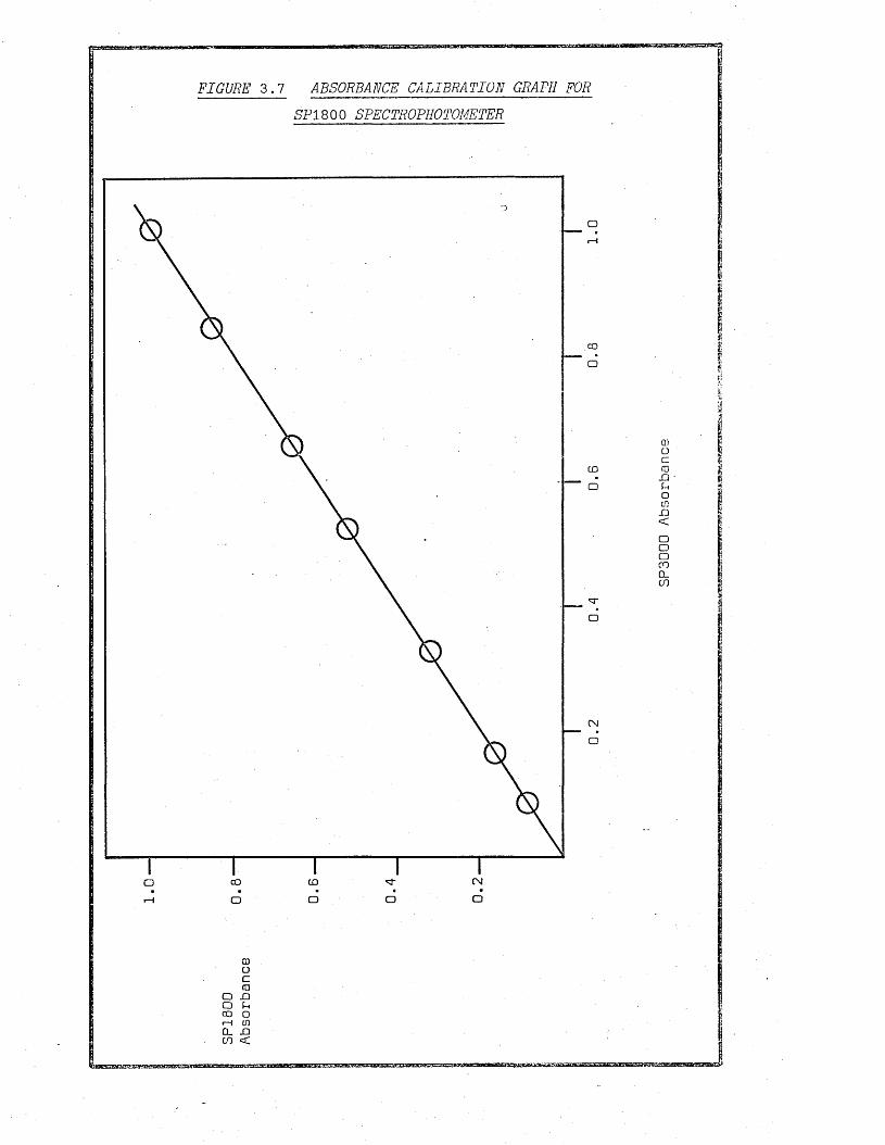
FIGURE 3.7 ABSORBANCE CALIBRATION GRAPH FOR SP1800 SPECTROPHOTOMETER
o
COo
co
COo CDo o □
aocfUXDuom1 3<r
SP3000 Absorbance

unukummmii
FIGURE 3.8 DRIFT OF HIGH TEMPERATURE SPECTROMETER
DURING WARM UP
CO
□
OCO
tokrjoDC
03E•Hh-
CD CD
0Oc<UJDUoCOJD<
Bw a M u aaas

CHAPTER 4
ASSOCIATION CONSTANTS OF VARIOUS LIGANDS AND A METAL COMPLEX
AS FUNCTIONS OF TEMPERATURE

4.1 INTRODUCTION
4.1.1 LIGANDS
Previous workers20-23 have studied the temperature dependence
of the acid dissociation constant of 2,2'-bipyridine and some
1,10-phenanthrolines at temperatures up to 225°C. . These compounds
are of interest because of their possible use as chelating agents
in high temperature boilers. The present work is an extension of
these studies to include two diacidic bases, two quinolines, and
two pyridines. One of the objects of this work is to provide more
precise values of AH° and AS° than are possible from measurements
made over smaller temperature ranges (usually < 25°C). Another
is to formulate equations to allow extrapolation of lower tempera
ture data to higher temperatures.
The general equation for association of a mono-acidic base
with a proton is given in equation (4.13
L + H+ t LH+ K2 (4.13
The two equations for association of a diacidic base with
two protons are given in equations (4.2a3 and (4.2b).
L + H+ J LH+ K-. (4.2a)
HL+ + H+ I K2 - (4.2b)
Diacidic bases are of interest because they offer the chance
to study the protonation of a positively charged species and to
investigate the way in which the doubly charged species behaves.
All the reactions studied in this chapter are isoelectric
and.so have very small electrostatic contributions to the free

energy of association. In consequence they all exhibit high
linearity in log(K) vs 1/T plots.
Prior to this work no association constants for diacidic bases
have been reported in the literature at temperatures greater than
90°C. A least squares computer program, SQUAD, is used in this
work to calculate the best association constants simultaneously
for each diacidic.base at each temperature and this represents a
considerable improvement over methods23 previously used for spectro-
photometric analysis at high temperatures, which were limited to
studies of monoacidic bases.
Conventional methods for the spectrophotometric determination
of association constants usually make use of buffer solutions of
known pH. Measurement of pH at elevated temperatures is extremely
difficult and this work followed the previous23 practice of using
solutions whose total hydrogen ion concentration was known but whose
pH at the time of the experiment was unknown.
4.1.2 THE COMPLEX ION BIS (2,2’,2” TERPYRIDINE) IRON HI)
This work is an extension of the studies by Alexander23*25
of the iron (II) tris-complexes of 1,10-phenanthroiine, 5-nitro-
1,10-phenanthroline and 2,2’-bipyridine. All these complexes
exhibited intense charge transfer bands in the visible region,
were low spin and significantly more stable than the corresponding
high spin bis- and mono-complexes. In effect the reaction being
studied was:
2+ -> 2+M + 3L CMLg] $ 2 overall stability constant.

These complexes are important in analytical chemistry91 and
much work has been published concerning them92'93.
The subject of the present studies was 2,2’,2'1-terpyridine,
a tridentate ligand (in contrast to the previous compounds) which
forms a low spin bis-complex with iron (II).
2,2',2’'-TERPYRIDINE
The bis-complex (iogK2=13.5)125 is considerably more stable
than the mono-complex (logK^=7.4)125 so formation of the mono-complex
may be ignored in solutions where the total 2,2’,2’’-terpyridine
concentration is twice the total iron (II) concentration. The
reaction being studied is thus:
M2+ + 2L t [ML2]2+
The bis-iron complex is of importance in analytical chemistry91*'95
where it has better sensitivity and freedom from interferences than
other complexes.
The reaction was followed by employing hydrogen ions to
compete with iron (II) for the ligand and the results analysed
using SQUAD (Chapter 2). All test solutions were degassed under

vacuum to prevent oxidation of the complex, which proved serious□at temperatures exceeding 30 C.
4.1.3 METHODS OF ANALYSING THE TEMPERATURE
DEPENDENCE OF ASSOCIATION CONSTANTS
The temperature dependence of association constants can be
treated in several ways. The most usual is to construct van't Hoff4 .
plots (log(K) vs 1/T (°K.)) and to analyse these to determine the
enthalpy, entropy and heat capacity changes accompanying the
reactions. Least squares computer techniques have been used to
fit equations to the logCK.) vs 1/T plots and thermodynamic parameters
have been calculated from the coefficients of the best-fit lines.
This discussion will be limited to three equations
-R£n(K) = y +' b (4.3)
-RAn(K) = y + b + c£n(T) (4.4)
-R£n(K) = y + b + cT (4.5)
Equation (4.3) assumes ACp° to be equal to zero, i.e. constant
AH° and AS° over the experimental temperature range. In this case:
IIoCD< a + bT
AH° = a
> cn o ii -b
ACp° = □
Equation (4.4) assumes a constant value for ACp° over the
temperature range. This is the much-used Everett Wynne-Jones
equation96. In this case:

AG° = a + bT + cT£nT
AH° = a - cT
AS° = -(b + c + c£nT). ^ oACp = -c
It can be seen that if ACp° = □ the equations'are identical
to those derived from equation (4.3).
Finally, equation (4.5) assumes ACp to be a linear function
of absolute temperature and is similar to that proposed by Harned
and Robinson97. In this case:
AG° = a + bT + cT2o 2AH = a - cT
AS° = -(b + 2cT)
ACp° = -2cT
Again, if ACp° = □, the equations revert to those derived
from equation (4.3).
Equation (4.3) is obviously applicable only to those systems
which exhibit a linear van’t Hoff plot. This is the case for most
of the organic bases and metal complexes studied by Alexander,
Buisson, Irving and the a.uthor and thus merits serious consideration
as a means of describing the temperature dependance of the association
constant in these systems. Equations (4.4) and (4.5) are applicable
to systems exhibiting non-linear van’t Hoff plots and involve
reasonable assumptions, although these are difficult to demonstrate.
Equation (4.5) is the easier to fit from a computational

standpoint as it is a simple polynomial in temperature and many
least squares polynomial-fitting programs are available. Equation
(4.4) requires the use of a generalised function minimisation
program and would probably take more time to implement than a
polynomial fitting program. This probably explains the use of
equation (4.5) in previous high temperature research22'23'24.
Equation (4.4) will not be considered further in this discussion
except to say that most of the remarks addressed to equation (4.5)
will apply to equation (4.4).
The choice lies now between equation (4.3) and equation (4.5);
the former giving a straight linerplot and the latter a curved plot.
Two previously investigated systems* will be considered, namely
2,2'-bipyridine22 and 1,10-phenanthrcline23*24.
It will be shown that equation (4.3) is the most suitable
equation to use and that the errors quoted for the association
constants in these determinations are too small owing to the neglect
of an additional source of error.
One of the equations used by Buisson22 and Alexander23 to
calculate the association constant of a monoacidic base is given
in equation (4.6)
log(K) = pHCI)+log((A(I)-Ao)/(Aco-A(I))) (4.6)
*Acid dissociation constants were measured in these cases.
pK = -log(K ) = log(K) a a
K = acid dissociation constant aK = association constant

K = association constant for the reaction.
ACI) = absorbance of solution I.
pH(I) = pH of solution I.
Aq = absorbance of a solution if all the ligand
were in the unprotonated form.
A = absorbance of a solution if all the ligand 00 0
were in the protonated form.
The standard deviation in log(K) was found by averaging the
separate values of log(K) produced by equation [4.6).
Use of this equation required Knowledge .of Aq and A^, both
experimental quantities, and therefore both subject to experimental
error. No account of these errors has been taken in calculating
the standard deviation in log(K).
In order to determine whether or not the calculations were
sensitive to errors in A and A , typical absorbance errorso 00(± 0.002 absorbance units) were introduced to the values of A andoA^ independently and together and the change in average K noted.
Table 4.1 shows the largest change in log(K) produced by
simultaneous changes of 0,002 absorbance units in Aq and A^. Values
of A and A in Table 4.20 were taken from reference 23 and applyo co
to 1,10-phenanthroline.
From this table it is apparent that deviations of ± 0.002
absorbance units in A and A give rise, on average, to deviationso 00of 0.015 log units in log(K). This situation also applies to the

results for 2,2'-bipyridine as the errors are a result of the method of
mathematical analysis rather than the particular system being
studied.
TABLE 4.1
CHANGES IN LOGiK) PRODUCED BY SIMULTANEOUS CHANGES OF 0.002 IN A AND A-------------------------------------------------------------------------- O --------------- oo
Temperature(°C3 A0 AOO
Maximum Change in logOG
25 1.027 0.151 0.012100 0.477 0.054 0.020125 0.811 0.077 0.014175 0.798 0.127 0.012200 0.482 0.065 0.019225 0.285 0.050 0.032250 0.971 0.440 0.015.....
Table 4.2 shows the deviations assigned to log(K) for 1,10-
phenanthrcline with and without allowance for errors in A and A .o 00Values without allowance are taken from -reference 23, page 97, and
values with allowance are calculated by adding 0.015 to the corres
ponding values without allowance and rounding to two decimal places.
Table 4.3 shows similar calculations for 2,2’-bipyridine based on
data from reference 22.
It is now clear that the deviations in log(K) are at best
0.02 log units, which are some 2 to 4 times greater than the originally
quoted values. This, in turn, calls into question the validity of
using equation (4.53 to describe the van't Hoff plots,
Occam's Razor states that when two or more explanations of
an event adequately describe that event, then the simplest explanation

should be chosen in preference to the others. In this case, the
two descriptions are equations (4.3) and (4.5).
TABLE 4.2
REVISED STANDARD DEVIATIONS IN LOGiK) FOR 1,10-PHENANTHROLINE
Temperature(°C) log(K) Deviation
Without Allowance.Deviation
.With.Allowance
25 4.812 0.008 0.0245 4.655 0.008 0.0286 4.388 0.010 0.03107 4.266 0.008 0.02150 4.02 0.01 0.03200 3.84 0.02 0.04250 3.68 0.10 0.12 .
TABLE 4.3
REVISED STANDARD DEVIATIONS IN LOG(Z) FOR 2,2'-BIPYRIDINE
Temperature(°C) log(K) Deviation
Without AllowanceDeviation
With Allowance
25 4.323 0.005 0.0235 4.226 0.005 0.0245 4.138 0.005 0.0265 3.98 0.01 0.0386 3.84 0.01 0.03107 3.72 0.01 0.03125 3.62 0.01 0.03150 3.50 - 0.01 0.03
, 175 3.39 o.oi • 0.03200 3.32 0.01 0.03
Tables 4.4 and 4.5 show, for 1,10-phenanthroline and 2,2'-
bipyridine, respectively, the experimentally determined values of
log(K) together with the larger deviations and the values of log(K)
calculated from the best fit parameters of equations (4.3) and (4.5).

TABLE 4.4
LOGVK) FOR 1,10-PHENANTHROLINE
Temperature(°C)
log(K) ...................
Calculated from Equation (4.3)
And Standard Deviation -
(Experimental)Calculated from Equation (4.5)
25 4.82 4.81(2) 4.8145 4.66 4.66(2) 4.6686 4.38 4.39(3) .4.38
107 4.26 4.27(2) 4.26150 4.05 4.02(3) 4.05200 3.85 3.84(4) 3.85250 3.70- 3.68(12) 3.69 .
TABLE 4.5
LOGiK) FOR 2,2*-BIPYRIDINE
TemperatureC°C)
'log(K)
Calculated from Equation (4.3)
And Standard Deviation
(Experimental)Calculated from Equation (4.5)
25 4.31 4.32(2) 4.3235 4.22 4.23(2) 4.2345 4.14 4.14(2) 4.1465 3.99 3.98(33 3.9886 3.85 3.84(3) 3.84
107 3.72 3.72(3) 3.71125 3.63 3.62(3) 3.62150 3.51 3.50(3) 3.50175 3.40 3.39(3) 3.40200 3.30 3.32(3) 3.31
A good indication of the suitability of an equation to a
set of data points is given by comparing the standard deviation of

between the observed and calculated (from the equation) points
with the typical errors associated with the points.
In this case the typical error associated with any point is
at best ± 0.02 log units and Table 4.6 shows the standard deviation
of fit, calculated from the sum of squares of residuals, for both
equations derived from the data in Tables 4.4 and 4.5. Data
precise to three decimal places has been used where possible to
avoid rounding errors.'
TABLE 4.6
STANDARD DEVIATIONS OF FIT FOR EQUATIONS (4.3) AND (4.5)
Compound Std. Deviation of Fit Std. Deviation of FitEqn. (4.3) Eqn. (4.5)
1,10-Phenanthroline 0.019 0.0192,2'-Bipyridine 0.009 0.005
It is clear from Table 4.6 that for 1,10-phenanthroline no
improvement in the sum of squares occurs when equation (4.5) is used
instead, of equation (4.3) and that equation (4.3).fits the experi
mental data to within one standard deviation. By applying Occam’s
Razor the two parameter equation (4.3) would be preferred to the
three parameter equation (4.5).
Table 4.6 shows that for 2,2’-bipyridine the fit for equation
(4.5) is approximately twice as good as that for equation (4.3).
However, equation (4.3) describes the experimental points to well
within their estimated errors (± 0.02) and it is suggested that the
better fit of equation (4.5) is quite meaningless in relation to

the estimated errors of the points. Again, Occam's Razor suggests
that equation (4.3) is to be preferred to equation (4.5).
Having established that equation (4.5) offers no advantage
over equation (4.3) in describing the experimental data in these
systems, it is clear that any discussion of the temperature variation
of the values of AH°, AS0 and ACp° as calculated from equation (4.5)
must be considered to be extremely unsound, since equation (4.3)
gives temperature invariant values of AH° and AS° with ACp° = 0.
o oPlots of AH against TAS using values obtained from equation
(4.5) have been used to support a,new application of the Compensation
Law98-100. The compensation law has its main application to the o ovalues of AH and AS obtained at a fixed temperature for a series
of carboxylic acids98 which differ primarily in the degree of
solvational changes accompanying ionisation. It is often found
that AG° can be related to the structure of the molecule as suggested
by Hammett, but it is usually impossible to relate AH° or AS° to the
molecular structure. This situation led.to the conclusion that AH°
and AS° contained contributions which cancelled out in ,AGQ and it
has been shown, in some cases, that almost complete cancellation
occurs98.
Values of AH° and AS° to be used in the conventional applica
tion of the compensation.law are obtained by application of equation
(4.5) or (4.4) to the data for each compound. . The values of AH°
and AS° are thus independent of each other. , The new application of
the compensation law by Buisson and Alexander to, say, 1,10-
phenanthroline uses values of AH° and AS° which are related to each

other by equation (4.5) and which are therefore not independent
of each other. In effect, when AH° is plotted against TAS; (a-cT2)2is being plotted against (bT + 2cT ) where a, b and c are constants
and T is the absolute temperature. If, as Alexander and Buisson
claim, a straight line is produced then it can be related to the
general equation for a straight line y = mx + K in which t2y = a-cT
m = slope, a constant
x = bT+2cT2
R = a constant (y axis intercept).
The slope should be a constant in this equation which can now
be formulated as:
a - cT2 = m(bT + 2cT2) + K
If T = 0
a - 0 = m ( 0 + 0 ) + k
.'. k = a
Thus a - cT2 = m(bT + 2cT2) + a
-cT b + 2cT
It is now clear that m is temperature dependent, and therefore
not a constant as previously claimed. Great care must, therefore,
be exercised in the interpretation of plots made from non-independent
variables. The discussions by Alexander and Buisson of their
results in terms of the compensation law must be considered to be
m = a - cT - a bT + 2cTz

questionable, especially when it is considered that temperatureo oinvariant values of AH and AS are sufficient to describe the
experimental data within the estimated error.
4.1.4 REVISED INTERPRETATION OF PREVIOUS RESULTS
In the light of the discussion in section 4.1.3 the results22
obtained by Alexander and Buisson for 2,21-bipyridine, 1,10-
phenanthroline, 5,6-dimethyl- and 5-nitro-l,10-phenanthrolines haveobeen re-analysed using equation (4.3), i.e. ACp = 0. The new
results are presented in Table 4.7.
The data for 2,9-dimethyl-l,10-phenanthroline has not been
re-analysed as this compound shows a marked curvature in its van't
Hoff plot which has been ascribed to steric effects23.
TABLE 4.7
RECALCULATION OF A if* A W A S° FOR COMPOUNDS STUDIED PREVIOUSLY AT'HIGH TEMPERATURES
Compound AH°(kJ.mol-1)
AS°(J.deg-1.mol"1.)
1,10-phenanthroline -15(1) 42(3)5,6-dirnethy 1-1,10-phenanthroline -27(1) 14(3)5-nitro-l,10-phenanthroline -11(1) 25(3)2,2’-bipyridine -15(1) 30(3)
4.1.5 CONCENTRATION SCALE
Discussions of concentration scales by Quist and Marshall101,
and Bell and Gat-ty102 concluded that the molar scale was the most
appropriate scale for use at high temperatures, since this scale
accounted for the temperature-volume properties of the solvent. In

consequence this scale has been adopted for use in this chapter
and to give compatibility with previous high temperature work21-25.
4.2 THEORY
4.2.1 COMPUTATIONAL METHODS
4.2.1.1 MOHOACIDIC BASES °
Previous investigations by Alexander23 and Buisson22 of mono-
acidic bases made use of a computational technique which was capable
of dealing with only one wavelength at a time. The present investi
gations make use of the computer program SQUAD . (Chapter 2] which is
capable of handling many wavelengths simultaneously.
When single wavelength data was processed by. Alexander and
Buisson’s technique and by SQUAD, identical results were obtained
within the standard deviations giver} by SQUAD.
The method of analysis in this work consisted of making up a
series of solutions of known total ligand and total hydrogen ion
concentrations. The absorbance of each solution at a number of
wavelengths was then measured at the experimental, temperature. This
data together with the total reagent concentrations was then input
to SQUAD, which found the value of association constant which best
described the given data.
4.2.1.2 DIACIDIC BASES
Prior to this work no diacidic bases had been studied at
temperatures greater than 90°C. Diacidic bases present much
greater computational problems than do monoacidic bases. This is
primarily due to the difficulty of determining the extinction

coefficient of the monoprotonated species.
For certain compounds with widely differing association
constants it is possible to find wavelengths at which changes in
absorbance are due to either one step or the other, but not both.
If this is the case then the two steps can be analysed separately
as two monoacidic steps. However.it is usual to find that no wave
lengths exist at which it is possible to make separate studies of
the two steps, which complicates matters considerably.. Three cases
can be demonstrated which differ only in the relative magnitudes
of the association constants of the two steps.
The first case is shown in figure 4.1 where the step associa
tion constants are widely separated. In this case the extinction
coefficient of the monoprotonated species can be determined and the
two steps treated individually as monoacidic steps.
The second case is shown in figure 4.2 where the step
association constants are closer than in-the first case. It is now
impossible to measure the extinction coefficient., of the monoprotonated
species directly as it is never present to more than 65%. This case
corresponds to" that found in the work on diacidic, bases in this
chapter. Various mathematical procedures have been developed51 for
circumventing this problem, but they are all single wavelength
techniques and are particularly difficult, to apply if the pH of the
solution is unknown. They also tend to give different answers at
different wavelengths.
The third case is shown in figure 4.3 in which the two step
association constants are equal. The concentration of monoprotonated

mumiM.'fc'J 'Ilf M i'i»! it'< TV'
FIGURE H.l SPECIES DISTRIBUTION DIAGRAM FOR A PI ACIDIC BASE WITH p K = 5.5 AND p K2 = 2.(9
LUCD 2 < O I— M S h- LU <u z: or dcLU O CL LL
pH of
Solution
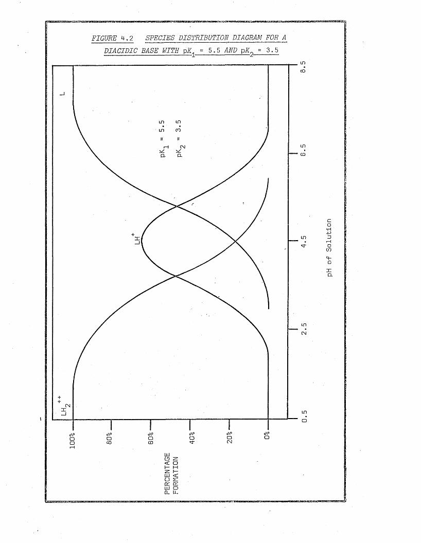
? a TiOTSMyaagq u ram taicBatt^'agsg sfiBsaaaKPtfffqggBfiE aiP iB ^ ^
FIGURE 4.2 SPECIES DISTRIBUTION DIAGRAM FOR A
PI ACIDIC BASE WITH pK = 5.5 AND p #2 = 3.5inCO
LDLDCO
LDCMHCLCL CO
LDX
inCM
CMin□
o\°oo\°oCM
o\°Oo\°oCD
o\°OCOo\°O
LLiCD X < O I— H X I— LLI < CD X
X X
pH of
Solution

FIGURE 4.3 SPECIES DISTRIBUTION DIAGRAM FOR
5.5 AND pK,A DIACIDIC BASE WITH pK.
incn
in ininin in
Q. Q.
in
CO
in
o\°o\°o\°o\° o\°ocno\°
CNCOi—i
CD OHLLICD
LLI O Q_ Ll_
pH of
Solution

species is now almost negligibly small and unless the extinction
coefficient of the monoprotonated species is considerably larger
than either the free base or the diprotonated species it is
extremely difficult to determine the two association constants of
the system.
The diacidic bases studied in this chapter fall into category
two and were analysed with the aid of the computer program SQUAD
(Chapter 2). This program has the advantages over previous methods
of needing only the total reagent concentrations of each solution
and of being able to process absorbance measurements from several
wavelengths simultaneously. ,
4.2.1.3 THE COMPLEX ION BIS (2,2',2’1-TERPIEIDINE) IRON {II)
Due to the very high value of. stability constant for the bis-
complex compared.to the mono-complex and the relative reagent
concentrations used, formation of the mono-complex was ignored in
calculating the stability constant of the bis-complex according to
equation (4.8).
Fe2+ + 2Te Z [FeTe232+ (4.8)
The stability constant of the complex is too high to be
studied by observing simp-le solutions of iron (II) and 2,2,,2,,~
terpyridine hence it was necessary to follow the reaction by observ
ing the competition between iron (II) and hydrogen ions for the
ligand. This introduces two further equations into the system.
+ ->• +L + H •*- HL+ + ?+ HL + H H2L
(4.9)

Before commencing this work the association constants for
reactions (4.9) were determined so that at any temperature only
the stability constant of equation (4.8) was unknown,- together
with the extinction coefficient of the bis-complex.
The computer program SQUAD (Chapter 2) was used to analyse
the system defined by equations (4.8) and (4.9)., The ligand
association constants at any temperature were given as non-variable
parameters and the absorbance measurements were made in a wavelength
region where only the iron (II) complex absorbed.. Thus the absorbance
measurements were linearly related (by the extinction coefficient)
to the concentration of complex and only .two Variable parameters,
extinction coefficient and stability constant of the complex, were
present.
4.2.2 CHANGES IN THE DENSITY OF WATER WITH TEMPERATURE
The.molar scale has been adopted for all work in this chapter.
In consequence, changes in the density of water between the tempera
ture at which the solutions were made up and the temperature at
which they were measured have to be taken into account.. The follow
ing formula was applied by SQUAD to room temperature concentrations
to obtain the concentrations at higher temperatures. These concen
trations were used in all further calculations. .
dTCT ,?Co X dI .o
= concentration (mol.£ ) at the experimental temperature.— 1 QC = concentration (mol.£ ) at 25 C. o
-3d.j. = density of water (g.cm ) at the experimental temperature and SVP.
d = density of water (g.cm ) at 25°C and 1 atm. pressure, o

Values for the density of water as a function of temperature
were taken from reference 90 and are also given in reference 23.
4.3 EXPERIMENTAL
4.3.1 ABSORBANCE MEASUREMENTS iT < §0°C)
A Pye Unicam SP3000 (ultraviolet-visible) automatic single
beam spectrometer was used at temperatures less than 90°C. The
claimed precision and reproducibility of this instrument is ± 0.001
absorbance units and long term drift was found to be ± 0.002
absorbance units per year by reference to National Physical Laboratory
calibrated absorbance standards.
The standard 1cm quartz cells were held in a cell block
through which water was circulated from a thermostated bath fitted
with heating and refridgerating elements. Temperature control was
± 0.2°C.
Few problems were experienced with this system except that
care was needed at temperatures less than 10°C.to avoid condensation
of water vapour, on.the windows. If this occurred, it was removed
with a clean paper tissue immediately before measurements were made.
At temperatures greater than 40°C air bubbles formed on the inside
surfaces of the cell and had to be shaken off. by gently tapping the
bottom of the cell.
4.3.2 ABSORBANCE MEASUREMENTS (T > 90°^)
The high temperature Pye Unicam SP1800 (ultraviolet-visible)
spectrophotometer described in Chapter 3 was used in the manner
described in that chapter. The calibration accuracy and reprcduci-

bility have also been described in Chapter 3. Temperature regulationoand indication were ± 1 C using calibrated chrome-alumel thermo
couples.
After filling the high temperature cell according to the
procedures detailed in Chapter 3, the cell was placed in the furnace
assembly and the absorbance monitored on a chart recorder. When
constant absorbance had been reached, typically after 12 minutes,
absorbance measurements using air as the reference were made at
predetermined wavelengths. When all the test solutions had been
measured the cell was filled with water and absorbance measurements
taken at the same wavelengths as for the test solutions.
4.3.2.1 CALCULATION OF TRUE ABSORBANCE VALUES (T > 90°C)
During the heating cycle small quantities of liquid sometimes
leaked past the teflon seals and evaporation caused deposits to be
left on the windows. The deposits had unknown absoroance values which
were found to be. . wavelength independent over the range 240-510nm.
Hence the absorbance measured at any wavelength by the spectrometer
contained a small unknown inaccuracy, typically less than 0.010
absorbance units.
The true absorbances of the solution could be found by
measuring the absorbance at a wavelength at which the compounds in
solution did not absorb, in addition to measurements at the wave
lengths of interest.. In conjunction with absorbance measurements of
the cell, when.filled with water, at identical wavelengths the
following procedure yielded the true absorbance values of the
solution.
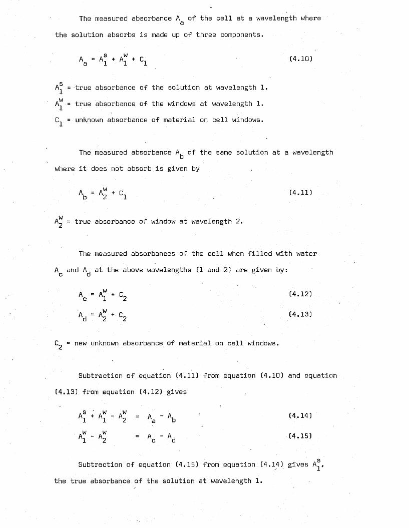
The measured absorbance A of the cell at a wavelength where0
the solution absorbs is made up of three components.
A = A® + A^ + C. (4.10)a 1 1 1
sA^ = -true absorbance of the solution at wavelength 1. wA^ = true absorbance of the windows at wavelength 1.
= unknown absorbance of material on cell windows.
The measured absorbance A^ of the same solution at a wavelength
where it does not absorb is given by
A, = A J + C. (4.11)b 2 1
wA^ = true absorbance of window at wavelength 2.
The measured absorbances of the cell when filled with water
Ac and A^ at the above wavelengths (1 and 2) are given by:
A = A“ + C„ [4 . 12]c 1 ^
A . = A^ + C„ (4.13)d 2 2
= new unknown absorbance of material on cell windows.
Subtraction of equation (4.11) from equation (4.10) and equation
(4.13) from equation (4.12) gives
A^ + A^ - A^ = A " A (4.14)1 1 2 a b
A* - A^ = A - A (4.15)1 2 c d
sSubtraction of equation (4.15) from equation (4.14) gives A^,
the true absorbance of the solution at wavelength 1.

Thus the true absorbance of the solution is given by:
= (A - A J - (A - A ) l a b c d
4.3.3 CHOICE OF ANALYTICAL WAVELENGTHS
Analytical wavelengths were chosen by a visual inspection of
spectra of the ligand in acid (0.1M HC£) and alkaline (0.01M NaOH)
solutions. The wavelength region in which the greatest spectral
changes were evident was chosen as the analytical region. In cases
where two regions were evident separated by a relatively invariant
region, no measurements were made in the invariant region.r '
4.3.4 PURITY OF REAGENTS AND STANDARDISATION
4.3.4.1 2,2’,2" -TERPYRIDINE
Source: Koch Light Chemical Company
Stated Purity: 99.0%
Melting Point: 78°C
Literature1^2: 80 C
The supplied material was recrystallised twice from hot
C65°C) distilled water and dried under vacuum.
Melting Point (Recrystallised Material): 78°C
Microelemental Analysis: see section 4.3.4.7.
4.3.4.2 4,4'-BIPYRIDINE
Source: BDH
Stated Purity: > 99.0%
Melting Point: 72°C

Literature187: 73°C
The material was used as supplied.
Microelemental Analysis:, see section 4.3.4.7.
4.3.4.3 8-AMINOQUINOLINE
Source: Eastman Kodak Company■I *
Stated Purity: 95%
Melting Point: 64°C
Literature187: 70°C
The supplied material was recrystallised twice from hot
C85°C) distilled water and dried under vacuum.
Melting Point'(Recrystallised Material]: 69°C
Microelemental Analysis: see section 4.3.4.7.
4.3.4.4 8-HYDR0XYQUIN0LINE
Source: Aldrich Chemical Company
Stated Purity: 99.5%
Melting Point: 75°C
Literature187: 75°C
The material was used as supplied.
Microelemental Analysis: see section 4.3.4.7.
4.3.4.5 2-AMINOMETHYLPYRIDINE
Source: Aldrich Chemical Company

Stated Purity: 99%
Boiling Point: 82°C at 12mm Hg
Literature187: 84° C at 12mm Hg
The material was used as supplied.
Microelemental Analysis: see section 4.3.4.7.
4.3.4.6 PYRIDINE
Source: Aldrich Chemical Company
Stated Purity: 99.5%
Boiling Point: 114°C
Literature187: 115°C
The material was used as supplied.
Microelemental Analysis: see section 4.3.4.7.
4.3.4.7 MICROELEMENTAL ANALYSIS
MaterialC C%) H [%) N C%) 0 [%)
Calc Found Calc Found Calc Found Calc Found
2,2*,2*’-ter- pyridine ' 77.3 77.4 4.7 4.6 18.0 18.0 0.0 0.04,4’-bi- pyridine 76.9 76.3 5.1 5.1 18.0 17.7 0.0 0.08-amino-quinoline 75.0 74.8 5.6 5.7 19.4 19.5 0.0 0.08-hydroxy-quinoline 74.5 74.6 4.8 4.8 9.7 9.8 11.0 10.82-aminomethyl-pyridine 66.7 65.3 7.4 7.3 25.9 25.3 0.0 2.1Pyridine 75.9 76.1 6.3 6.5 17.8 18.1 0.0 0.0

4.3.4.8 ACIDS AND ALKALIS
Sodium hydroxide and hydrochloric acids were of AnalaR quality
supplied by B.D.H. The acid was standardised against borax accord
ing to Vogel103 using methyl red as indicator. Sodium hydroxide
was standardised against the standardised acid using methyl red
indicator.
fV
4.3.4.9 IRON [II) SULPHATE HEPTAHi DRATE
Iron (II] sulphate heptahydrate (BDH.AnalaR) was used without -
further purification. Stock solutions were prepared of about -31.0x10 M concentration and to suppress hydrolysis sufficient
hydrochloric acid was added to attain pH 'v 2.5. Each stock solution
was standardised oxidimetrically against standard eerie sulphate
using N-phenylanthranilic acid as indicator according to Vogel101*.
4.3.4.10 WATER
All water used in this work was singly distilled and de
ionised with a conductivity of'< 0.5y mho. No precautions were
taken to reduce the oxygen level in the water except, in the case of the
ion, bis (2,2',2''-terpyridine) iron CII1 when solutions were de
gassed under vacuum for 'v 1 min.
4.3.5 GLASSWARE AND OPTICAL CELLS
All volumetric flasks and pipettes were calibrated and soaked
in DEC0N-75 before use. DECON residues clinging to the sides of
volumetric flasks after, long periods of standing were removed with
concentrated nitric acid.
A matched pair of 1cm optical cells were used at temperatures

-below 100°C. These were stored in de-ionised water when not in
use and.calibrated for path length and absorbance blank, periodically.
At temperatures greater than 100°C the optical cells described
in Chapter 3 were used.O
4.3.6 PREPARATION OF TEST SOLUTIONS
4.3.6.1 LIGANDS
A stock solution was prepared from a weighed amount (a 0.2g)3
of ligand each day. The ligand was dissolved in ethanol (10cm 36%)
except for pyridine which was dissolved in de-ionised3 3water (10cm ). This solution was transferred to a 100cm volumetric
flask which was then filled to the mark with de-ionised water.
3An aliquot (10cm ) of stock ligand solution was then trans
ferred to each of six (monoacidic bases) or eleven (diacidic bases)3
volumetric flasks (100cm ). Aliquots from previously prepared
stock hydrochloric acid solutions were then added to the volumetric
flasks to give a range of hydrochloric acid concentrations which
were chosen to cover the range where the ionisation or ionisations
of the bases took, place. .Sodium chloride solution was then added
if necessary to maintain a constant ionic medium and the solutions
made up to the mark.
4.3.6.2 THE COMPLEX ION, BIS (2,2*2 ’’-TERPYRIDINE) IRON III)
Aliquots of stock iron (II), 2,2’,2''-terpyridine and hydro-3
chloric acid solutions were pipetted into a 100cm volumetric flask
and the solution made up to the mark.

Early experiments indicated the need to reduce the oxygen
concentration in solution to prevent oxidation of the complex.
Various methods were investigated including the use of ’boiled
water’, bubbling nitrogen through the solution and vacuum degassing.
Of these, vacuum degassing proved to be the quickest and most
effective method. °
The same degassing procedure was followed irrespective of
which optical cell was being used. However, the methods of filling the
cells did vary. The degassing procedure was performed on a nitrogen/
vacuum line originally developed to facilitate the preparation of
air-sensitive compounds. No description of this apparatus is
considered necessary except to say that it provided a means of
evacuating the experimental apparatus and filling it with de
oxygenated 'white spot’ nitrogen through a single connection.
The apparatus used to degas the test solutions is shown in
figure 4.4. Initially, taps A and D were opened with B and C
closed and the system evacuated and nitrogen-filled three times.
Secondly, taps B and C were opened together with taps A and D and
the whole system subjected to vacuum for 60 seconds. . Thirdly, tap
A was closed with taps B,.C and D open and nitrogen allowed to
enter the vessel slowly, via tap B. This forced the test solution
through taps C and D into the 1cm low temperature spectrophotometric
cell. Tap D was then closed and tap A opened to allow the solution
to drain back into the main vessel under an atmosphere of nitrogen.
Finally taps B and C were closed, sealing the test solution under
an atmosphere of nitrogen. The 1cm cell was then disconnected at
joint E and placed in the low temperature spectrometer complete

aj
FIGURE A. A DEGASSING APPARATUS
A
To Vacuum Line
sW/
□cm CellCone Joint
Test Solution

with tap D. The remainder of the apparatus was then disconnected
from the nitrogen line.
The high temperature cell was filled in the following manner.
The solution was degassed as described above, the apparatus filled
with nitrogen and taps B and C closed. This apparatus, together
with a high temperature cell, was then placed in a glove bag which*'*
was evacuated and filled with nitrogen six times. The cone joint
of the degassing apparatus (figure 4.4] was then parted allowing
access to the degassed test solution and the high temperature cell
filled and assembled, as indicated in Chapter. 3. The glove bag was
then opened and the cell transferred to the high temperature spectro
meter...
A degassing time of 60 seconds was found to result in a loss
of 1.4% of the solvent (water] and this was taken into account when
the results were processed by SQUAD.
This procedure resulted in no detectable oxidation occurring
at the highest temperature used (200°C] compared to non-degassed
solutions which showed marked oxidation at 30QC.
The small additional concentration of hydrogen ions present
in the stock solution of iron (II] was taken into account when the
total hydrogen ion concentration of the solution, was calculated.
4.3.7 EXPERIMENTAL CONDITIONS
Table 4.8 shows the temperature range over "which the ligands
were studied and whether the experiments were performed at constant
ionic strength.

TABLE 4.8
TEMPERATURE RANGE AND IONIC STRENGTH OF LIGAND STUDIES
LigandLowest
TemperatureC°C)
HighestTemperature
C°C)
Constant Ionic
. Strength
2,2’,2'’-Terpyridine 25 200° 0.05M NaC£4,4'-Bipyridine 5 175 0.05M NaC£8-Aminoquinoline 5 125° -
8-Hydroxyquinoline . 5 125° -2-Aminomethylpyridine 5 100 0.051*1 l\IaC£Pyridine 5 200 . -
D - temperature limited by ligand decomposition.
Table 4.9 shows the number of solutions and the ligand con
centrations used at each temperature whilst Table 4.10 shows the
acid concentrations used at the highest and lowest temperatures.
Table 4.11 shows the analytical wavelengths chosen.
TABLE 4.9
NUMBER OF SOLUTIONS AND LIGAND CONCENTRATION USED AT EACH TEMPERATURE
Ligand Number of Solutions
Concentration of.Ligand
2,2',2’’-Terpyridine 11 5.3x 10_5M4,4*-Bipyridine 11 6.8x 10“ 5M8-Aminoquinoline .6 3.0x10"^8-Hydroxyquinoline 6 4.0x10"^2-Aminomethylpyridine 7 . 2.0x10“Pyridine ...... 6 . . . 2.0x10“^ . . .

TABLE 10
ACID CONCENTRATIONS USED AT'THE HIGHEST AND LOWEST'TEMPERATURES
LigandAcid Concentrations Lowest.Temperature. .
Acid Concentrations . Highest.Temperature
Lowest. Highest Lowest. .Highest
2,2',2'’-Terpyridine4,4’-Bipyridine8-Aminoquinoline8-Hydroxyquinoline2-AminomethylpyridinePyridine
2.0x 10“5M 2.0x 10"5I4 5.0x 10⁻⁵M 5.0x10-^ 2.0x 10"4M 2.0x 10"51v]
2.0xl0“2M2.0x 10"2I42.0x 10“3H.2.0x10-3145. oxio~2ri 1.0x10-314
5.0x10"5M 5. 0x10" 5I4 1.0xl0"4f4 5.0x 10_5I4 5.0x10-^14 5.0x 10"5I4
5. 0x 10-2I4 5.0x 10"2I4 5.0x 10"3M 2. 0x10“ 3[4 5.OxlO-^M 2.0xl0"3l4
TABLE 4.11
ANALYTICAL WAVELENGTHS USED FOR EACH COMPOUND
LigandWavelengths (nm)
Number Start Finish In Stepsof Reference
2,2’,2’’-Terpyridine 10 270 315 5 5104,4'-Bipyridine 10 240 290* 10 5108-Aminoquinoline 6 295 345 10 5108-Hydroxyquinoline 10 270 360 10 5102-Aminomethylpyridine 6 230 280 10 510Pyridine 6 240 265 5 510
*Additional wavelengths 360, 380, 400, 420nm.
4.3.7.1 PIACIDIC BASES
Both 2,2',2V'-terpyridine and 4,4'-bipyridine necessitated
the use of relatively high acid concentrations at higher temperatures
and so.determinations of these association constants were made at a

constant ionic strength of 0.05M made up with sodium chloride.
Reference to the literature105 indicated that no protonation
of the third 2,2’,2’'-terpyridine nitrogen atom would be expected
to occur under the experimental conditions employed in this work.o
*1.3 .7 .2 M O W ACIDIC BASES EXCEPT 2-AMINOMETHYLPYRIDINE
Pyridine was monoacidic under the conditions of the experiments.
The heterocyclic nitrogen atoms of 8-aminoquinoline and 8-
hydroxyquinoline have been shown to be the sites of first protonaticn
in the neutral molecule106-109. The amino nitrogen atom of 8-
aminoquinoline (a, figure 4.5) is too weak a base ClogK = -0.13)110
to interfere with protonation of the 'heterocyclic nitrogen atom
Cb, figure 4.5) and this system will be treated as having two non-
overlapping steps, each of. which can be studied separately.
FIGURE 4.5
8-AMINOQUINOLINE
The hydroxyl group (a, figure 4.6) of 8-hydroxyquinoline is
too weak an acid ClogK = 9.8)111 to be ionised under the experimental
conditions and like 8-aminoquinoline, 8-hydroxyquinoline will be
treated as a monoacidic base.
FIGURE 4.6
8-HYDROXYQUINOLINE
OH(a)
Cb)
( b )

U.S.7.3 7-AMINOMETHYLPYRIDTNE
The amino nitrogen atom (a, figure 4.7) of 2-aminomethylpyridine
is much more basic. (logK = 8.78 at 20°C)111 than.the ring nitrogen
atom Cb, figure 4.7) and in,consequence the amino nitrogen atom will
protonate before the.ring nitrogen atom.
FIGURE 4.7
2-AMINOMETHYLPYRIDTNE
Calculations indicated that the values of the two association
constants were sufficiently far apart for the reactions to be
treated as two monoacidic steps in which the amino nitrogen atom
protonated fully, before the ring nitrogen atom.
-3Thus if a quantity of acid, say 1.0x10 14, was added to a-4solution which contained 2-aminomethylpyridine C2.0xl0 M) it was
assumed that 100% association would occur for the amino nitrogen
atom and that the effective total acid concentration would be re--4 -4duced by 2.0x10 M to give 8.0x10 M.
Cb)CH.
NH.(a)'
The reaction studied for 2-aminomethylpyridine is thus the

protonation of a protonated ion.
CH+NH
CH
4.3.7.4 THE COMPLEX ION BIS (2,2' ,2" -TERPYRIDINE) IRON (IX)-5Each solution contained iron (II) (8.0x10 M), 2,2,,2''-
-4terpyridine (1.6x10 Ml, hydrochloric acid (0.01 to 0.1M) and
sufficient sodium chloride to achieve a formal ionic strength of
O.IM. Six solutions were prepared for each determination and were
measured at six wavelengths, namely,
520nm
530nm
540nm
550nm
560nm
570nm
The temperature range studied was 25°C to 200°C.
Excess 2,2’,211-terpyridine over that required for a 2:1 ligand
metal complex was avoided as this would contribute nothing useful to
the determination and would reduce the effective acid concentration
by its need to be protonated before competition with iron (II) could
take place.
The reference wavelength was 700nm.

4.3.8 ANALYSIS OF MEASURED ABSORBANCE VALUES
When the experimental part of a determination had been
completed the following data was available.
(1) The number of solutions used, ’INT.
(2) The total metal (if present), ligand
and acid concentrations of each solution.
(3) The number of wavelengths used, ’IT.
(4) '14' x ’N' absorbance values.
This data was then transferred to punched cards, together
with the stoichiometries of expected complexes, initial guesses for
the values of the association constants and codes to indicate which
extinction coefficients were to be varied during the minimisation.
The data deck was then run through the computer program SQUAD
(Chapter 2).
The output from SQUAD consisted of values of the association
constants and extinction coefficients together with estimates of
their standard deviations. These values were calculated for three
cases (Chapter 2).
(1) All the solutions.
(2) All the solutions except that which
contributed most to the sum of squares.
(3) All the solutions except the two which
contributed most to the sum of squares.
Standard deviations and sums of squares for.the three cases
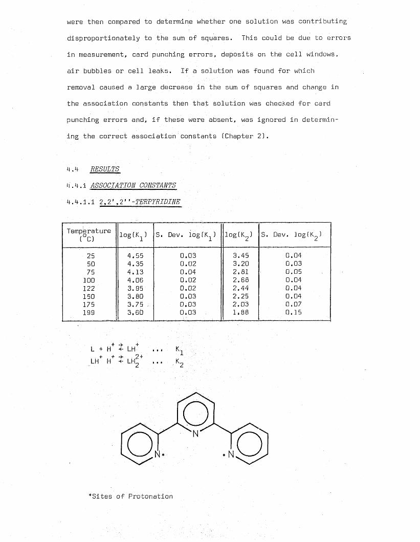
were then compared to determine whether one solution was contributing
disproportionately to the sum of squares. This could be due to errors
in measurement, card punching errors, deposits on the cell windows,
air bubbles or cell leaks. If a solution was found for which
removal caused a large decrease in the sum of squares and change in
the association constants then that solution was checked for card
punching errors and, if these were absent, was ignored in determin
ing the correct association constants (Chapter 2).
4,4 RESULTS
4.4.1 ASSOCIATION CONSTANTS
4.4.1.12,21,2 *'-TERPYRIDINE
Temperature(°C) log(K1) S. Dev. log(K^) log(K23 S. Dev. logfK^}
25 4,55 0.03 3.45 0.0450 4.35 0.02 3.20 0.0375 4.13 0.04 2.81 0.05100 4.06 0.02 2.68 0.04122 3.95 0.02 2.44 0.04150 3.80 0.03 2.25 0.04175 3.75 , 0.03 2.03 0.07199.....— 1
3.60 0.03 1.88 0.15
L + H LH • • * K-,+ + 2 +LH H LH2 K2
*Sites of Protonation

4.4.1.2 4,4’-BIPYRIDINE
TemperatureC°C) log(K1) S. Dev. logCK ] logCK^ S. Dev. log(K2)
5 4.96 0.04 3.09 0.0415 4.87 0.05 2.95 0.0625 4.80 0.04 2.94 0.0437 4.50 0.03 2.93 0.0550 4.44 0.02 2.79 0.0375 4.28 0.02 2.54 0.04100 4.07 0.02 2.29 0.06125 3.86 0.02 2.14 0.05150 3.69 0.03 1.90 0.07175 3.56 0.03 1.87 .. 0.07 .
+ +L + H ■*- LH .... K+ + 2 +LH + H -e- LH2 .... K2
*
*Sites of Protonation
4.4.1.3 8-AMINOQUINOLINE
oTemperature I CJ | log(K) S. Dev. logOO
5 I 4,19 0.0215 4.07 0.0225 3.95 0.0237 3.82 0.0250 3.67 0.0275 3.46 0.02
100 3.26 0.02125 3.13 0.05
+ ->• + L + H LH
N H 2*Site of onatior-

4.4.1.4 8-HYDROXYQUINOLINE
oTemperature C.CJ . log(K) S. Dev. .log(K).
5 5.14 0.0215 5.02 0.0225 4.88 0.0250 4.55 0.0275 4.28 0.02100 4.09 0.02125 3.81 0.04
+ -> + ■ L + H LH
OH*Site of Protonation
4.4.1.5 2-AMINOMETHYLPYRIDINE
Temperature C°C) log C K 3 S. Dev. log(KJ
5 2.03 • 0.0215 2.00 0.0225 1.96 0.0237 1.90 0.0250 1.80 0.0275 1.63 0.02
100. 1.46 .0.03
+ + -> 2+ LH + H LH^
nh2*Site of Protonation

4.1.6 PYRIDINE
0Temperature I Cj log(K) S. Dev..logCK)
5 5.51 0.0215 5.35 0.0225 5.20 0.0250, 4.92 0.0270 4.68 0.02
100 4.36 0.04125 4.18 0.02150 4.04 0.03175 3.90 0.04200 3.68 0.08
+ -> + L + H <- LH
*
. *Site of Protonation
4.4.1.7 THE COMPLEX ION BIS (2,2',2 ” -TERPYRIDINE) IRON ill)
Temperature C°C) log(82) S. Dev. log(82)
25 20.40 0.0849 19.32 0.1066 18.12 0.09100 16.69 0.08125 15.67 0.10149 14.68 0.12174 13.90 0.10199 13.19 0.10

M + 2L «- ML2 ... 3
Overall stability constant is 3,
M + L ML
ML + L -e ML,
K1 >< K2
... K,
4.4.2 VAN'T HOFF PLOTS
Van't Hoff plots (log ^CK) against 1/T ( K)) are shown as
follows:
2,2',2''-Terpyridine
4,4 ’-Bipyridine
8-Aminoquinoline
8-HydroxyIquinoline
2-Aminomethylpyridine
Pyridine
figure 4.8
figure 4.9
figure 4.10
figure 4.11
figure 4.12
figure 4.13
The complex ion bis (2,2’,2’’-terpyridine) iron (II) figure 4.14
4.4.3 ENTHALPY AND ENTROPY OF REACTION
4.4.3.1 LIGANDS
TABLE 4.12
PROTONATION ENTHALPYS. AND ENTROPYS OF VARIOUS COWOUNDS
Compound AH° _1 CkJ.mol. )
..j(J.deg. mol. )
2,2’,2’’-Terpyridine (Kl) -14(1) 40(3)2,2’,2’’-Terpyridine CK23 -24(1) -15(3)4,4'-Bipyridine CKlJ -20(2) 23(3)4,4'-Bipyridine (K2) -19(2) -2(3)8-Aminoquinoline -19(1) 12(3)8-Hydroxyquinoline -23(1) 15(3)Pyridine ............ . . . -22(1) . . ..... .25(3)......

FIGURE 4 .8 VAN'T HOFF PLOT OF 2,2' ,2" -TERPYRIDINE
This Work
Log(K)
4.0
2.0
2.0

FIGURE 4.9 VAN'T HOFF PLOT OF 4 , 4 -BIPYRIDINE
5.0*
Log(K)
4.0.
3.0 —
2.0'
This Work
Reference 115
| j Reference 114
2.0 L 3.0 3.5
1/T C°K) x 103

FIGURE 4.10 VAN'T HOFF PLOT OF 8-AMINOQUINOLINE
4.5 —
Log(K)
4.0__
3.5-
3.CT
This Work
O Reference 116
□ Reference 117
AOReference 118
Reference 119
2.0 2.5 3.0 3.5
1/T (°K) x 103

FIGURE 4.11 VAN'T HOFF PLOT OF
8-HIDROXYQUINOLINE
Log(K) This Work
Reference 120 *
^ Reference 121 ' ^
5.0— - Reference 122
- / \ Reference 123
| j Reference 120 and 124 /
4.5 — 1 /4.0 /
70
3.5 —
21 1 1.0 2.5 3.0 . 3.5
1/T (°K) x 1C3

1FIGURE 4.12 VAN'T HOFF PLOT OF
2 -AMINOMETHYLPYRIDINE
Log(K)
2.0
O This Work
| | Reference 125
O Reference 126 and 127 □
1.5
1.0 —
2.0 2.5 3.0 3.5
1/T C°K3 x iO3

FIGURE 4.13 VAN'T HOFF PLOT OF PYRIDINE
This Work
□ Reference 125
O Reference 128
A Reference 129LogCK]
Reference 131
4.0
3.02.0

r.rrjjtiT am 'gwraaw.’x
FIGURE M . 14 VAN'T HOFF PLOT OF THE COMPLEX ION
BIS {2,2’,2’’-TERPYRIDINE) IRON (II)
20.0_
Log(K)
18.0
16.0 —
14.0
1/1 (°K) x ID3

4.4.3.2 THE COMPLEXION BIS (2,2*,2'’-TERPYRIDINE) IRON ill)
TABLE 4.13
AH°-1 (kJ.mol. ]AS0
(J.deg.“Imol■ 3
113(9] 13(4]
4.5 DISCUSSION
4.5.1 COMPARISON WITH LITERATURE VALUES
4.5.1.1 2,2*,2’’ -TERPYRIDINE
Table 4.14 shows values of logCK^) and log(l<2] determined by
previous workers.
TABLE 4.14
VALUES OF PROTON ASSOCIATION CONSTANTS FOR 2,2’,2’1-TERPYRIDINE
TemperatureC°C] Ionic Strength logf^] log(K2] log(32] Reference
23 0 4.33(3] 2.64(7] 6.99(7] 10525 0.01 4.66(1] 3.28(3] 7.94(3] 11225 ? 4.69 3.99 8.68 11325 0.05 4.55(3] 3.45(4] 8.00(4]. This Work
The results obtained in this work are in reasonable agreement
with those of Offenhartz and George112, in particular the values of
It is not surprising that the values of and are less well
defined than 82 as-these are inter-related by the extinction coefficient
of the rnonoprotonated complex. A quantity which is impossible to -
measure directly in .this system. All previous determinations in
volved the use of questionably accurate extrapolations or manual

curve fitting. Martin and Lissfelt1s105 determination apparently
involves the use of an assumed, rather than calculated, value for
the extinction coefficient of the monoprotonated species and so
must be considered unreliable. James and Williams113 have used a
pH titration technique but do not. give details of their analysis
and their value for is in serious disagreement with this work.
r ■
The only literature values for AH° and AS° in this system
' are those of Offenhartz and George112 given in Table 4.15.
TABLE 4.15
ENTROPY AND ENTHALPY OF PROTONATION FOR 2,2’,2” -TERPYRIDINE
AH° CK1) kJ.mol"1
AS0 C^)J .deg.^mol.”1
AH° (K2) kJ.mol-1
AS° (K2)J.deg.-1mol.-1
Reference
-3-14(1)
7940(3)
-28-24(1)
-33-15(3)
112 This Work
4.5.1.2 4,4* -BIPYRIDINE
TABLE 4.16
PROTON ASSOCIATION CONSTANTS FOR 4,4'-BIPYRIDINE
Temperature(°C) Ionic Strength log(K1) log(K2) log(32) Reference
20.0 0.2 4.82 3.17 7.99 11418.8 0.1 4.83 2.73 7.56 11525.0 0.1 4.77 2.69 7.46 11531.5 0.1 4.70 2.62 7.32 11540.0 0.1 4.60 2.57 7.17 11525.0 ....0.05 4.80(4). 2.94(4). . .7.74. . This Work

Good agreement exists for between the present work and
literature values. This is not the case for where the value
obtained in this work at 20°C falls midway between the two literature
values which are widely separated. The K2 values from reference
115 are consistently 0.3 log units lower (figure 4.9) and this can-
• not be readily explained.
The values given in Table 4.16 from reference*115 allow AH°
and AS° to be calculated, these values are presented in Table 4.17.
TABLE 4.17 v
ENTHALPY AND ENTROPY OF PROTONATION OF 4,4'-BIPYRIDINF
AH° (K ) AS° (K ) AH° (K ) AS° (K ) ReferencekJ.mol-1 J.deg.-1mol.-1 kJ.mol-1 J.deg.-1mol.-1
-21 20 -14 5 115-20(2) 23(3) -19(2) -2(3) This Work
Reasonable agreement is evident hepe except for the AS° values
for which are influenced by the consistently lower values of
from reference 115.
4.5.1.3 8 -AMINOQUINOLINE
Table 4.18 shows the literature values for this system.
Good agreement is obtained with the exception of reference
119 which is neither consistent with the present work nor other
literature values (figure 4.10).

TABLE 4.18
PROTON ASSOCIATION CONSTANTS FOR 8-AMINOQUINOLINE
Temperature (°C) Ionic Strength log.(Kl.. . Reference
5 0.01 4.21 1165 0.003 4.19(2) This Work
20 0.02 3.95 11720 0.1 4.04 11820 0.003 3.99(2) This Work25 0.05 4.08 11925 0.003 3.95(2) This Work35 0.01 3.83 116
: 35 0.003 .3.82(2) This.Work
Values of AH° and AS° can be calculated from reference 116
and are shown in Table 4.19.
TABLE 4.19
ENTHALPY AND ENTROPY OF PROTONATION OF' 8-AMINOQUINOLINE
AH° (kJ.mol.-1) AS° (J.deg.-1mol._1) Reference
-22 3 116-19(1) 12(1) This Work
Good agreement is obtained for AH°, the difference in AS° is
explicable by the small temperature range and long extrapolation
used in its calculation from reference 116.
4.5.1.4 8-HYDROXYQUINOLINE
Table 4.20 shows the literature values for this system.
Good agreement is obtained except for references 121 and 122
which are nearly thirty years old (figure 4.11).

TABLE *+.20
PROTON ASSOCIATION CONSTANTS FOR Q-HYDROXYQUINOLINE
Temperature (°C) Ionic Strength log(K) .. Reference
20 0 5.02 12020 0.004 5.11 12120 0.02 5.09 12220 0.1 4.88 12320 0.003 4.93(2) This Work25 0 < 4.91 12025 0.5 4.91 1242 5 ....... 0.003 4.89(2)•■ This Work
AH° and AS° values are given in Critical Stability Constants
by Smith and Martell and are shown in Table 4.21.
TABLE 4.21
ENTHALPY AND ENTROPY OF PROTONATION OF 8-HYDROXYQUINOLINE
AH° (kJ.mol."1) AS° (J.deg._1mol. *) Reference.
-21 25 125-19(1) 12(1) This Work
Very good agreement is obtained for AHQ and the discrepancy
in AS° is attributable to the short (20GC) temperature range over
which the value from reference 125 was calculated.
4.5.1.5 2-AMINOMETHYLPYRIDINE
Table 4.22 shows literature values for this system.
125
+ + 2+ LH + H -f- LH2 K

TABLE 4.22
PROTOE ASSOCIATION CONSTANTS FOR 2-AMINOMETHYLPYRIDINE
oTemperature ( C) . . Ionic Strength .log(K) .. Reference
25 O.D5 1.96(2] This Work25 0.1 2.00 12525 0.5 2.25 12525 1.0 2.46 12525 0.1 2.14 12625 . 0.1 2.14.... 127
This equilibrium is much more ionic-strength sensitive than
systems such as 8-aminoquinoline, 8-hydroxyquinoline or pyridine.
Insufficient data precludes a comparison with the second protonations
of 2,2',2''-terpyridine and 4,41-bipyridine but the value for
log(K) of 1.96 obtained in this work is consistent with the trend
of decreasing K with decreasing ionic strength indicated in
reference 125. No explanation is evident for the value of 2.14
found in references 126 and 127 [figure 4.120.
Values of AH° and AS° are shown in Table 4.23.
TABLE 4.23
ENTHALPY AND ENTROPY OF PROTONATION OF 2-AMINOMETHYLPYRIDINE
Temperature [QC] AH° (kJ.mol."1] AS° (J.deg.-1mol.-1) Reference
25 -12 2 12525 -8(7) -10(6)........ This.Work
This system exhibits a non-linear Van't Hoff plot in contrast
to the remainder of the ligands studied in this chapter. ACp° is,
therefore, not 0 in this case and has a value of approximately

o20DJ.deg. mol. over the temperature range 5-50 C and
20J.deg. ^mol. 1 over the range 50-100°C.
4.5.1.6 PYRIDINE
Table 4.24 shows literature values for this system.
TABLE 4.24f ■
PROTON ASSOCIATION CONSTANTS FOR PYRIDINE
Temperature (°C} Ionic Strength. . log(K) . . Reference
20 0.15 5.32 12820 0.03 5.29 12920 0.005 5.30(2) This Work25 0 5.23 12525 0.005 5.21 13025 0 5.18 13125 . 0.005 5.21(2) .This Work
Very good agreement is evident at both temperatures reported
in the literature.
Values for AH° and AS° are given in Table 4.25.
TABLE 4.25
ENTHALPY AND ENTROPY OF PROTONATION FOR PYRIDINE
AH° (kJ.mol;-1) AS° (J.deg. 1mol.“1). Reference
-20(1) 31(7) 125-22(1) . .......25(3)......... .This Work.
Again, reasonable agreement with literature values is found.

4. 5 .1.7 THE COMPLEX ION BIS (2,2 ’ , 2 ’ '-TERPYRIDINE) IRON [II)
Table 4.26 shows literature values for this system.
TABLE 4.26
ASSOCIATION CONSTANTS FOR THE COMPLEX ION BIS (2,2’,211-TERPYRIDINE) IRON [II)
,0 .Temperature C Cj Ionic Strength log(£23 Reference
25 0.1 20.4 Cl) This Work23 0.1 20.4 13220 ? . 18.0. . .133
Good agreement is obtained .with the result of Martin and
Lissfelt132 suggesting that the value of Brandt and Wright133 is
incorrect. Few details of their determination are given making
analysis of their method impossible.
The value of log(K) = 20.4 found by Martin and Lissfelt was4 +for a complex of the formula [Fe(Te)2H2] in contrast to the
2 +formula FeCTe)2 used in this work. This is almost certainly an
error because the solid complexes [Fe(terpy)2]X2 have diffuse
reflectance absorption spectra in the visible and ultraviolet
regions which are identical to the spectra of the solutions from
which they were obtained* In addition, attempts to refine the
experimental data from this work in terms of the complex 4 +[Fe(Te)2H2] almost always led to convergence problems.
No literature determinations of AH° and AS° have been found,
preventing comparison with this work.

4.5.2 COMPARISON OF SQUAD WITH PREVIOUS COMPUTER PROGRAMS
Previous studies of the types described in this chapter have
been performed by Alexander23 and Buisson22 and for each type of
equilibrium, i.e. monoacidic base or tris-ligand metal complex,
a separate computer program has been written. These programs are
relatively small C300 lines of FORTRAN] and use a Newton-Raphson
iterative inner loop to solve the combined mass balance equation
and an iterative linear least squares treatment in an outer loop
to refine the equilibrium constant of the system. Their main
advantage is ease of use, but they have several disadvantages.
Firstly, each solution is measured at only one wavelength,
so that each solution gives only one data point. Secondly, major
changes to the program are necessary whenever the stoichiometry of
the system under study is changed. Thirdly, programs of this type
need three or more nested iterative loops when overlapping equilibria
are studied and have been found to be unstable and divergent.
Finally, the extinction coefficients of one or.more species must be
determined in order to run the program. This, in turn, means that
whenever an extinction coefficient, such as is often the case for
the monoprotonated species of a diacidic base, cannot be measured,
another iterative loop must be incorporated into the program leading
to greater instability problems.
SQUAD posesses several considerable advantages over the
previous type of program. Firstly, absorbance data from several
wavelengths can be processed simultaneously which tends to average
any spectrometer errors and may also show the presence of minor
species not accounted, for in the list of expected complexes given

to the program. Secondly, the number and stoichiometry of the
expected complexes can be varied at will by varying the input data;
no modifications are necessary to the program. Thirdly, overlapping
equilibria can easily be accommodated without need to alter the
program. Finally, extinction coefficients may be given for any
species for which they are available, but ,it° is not necessary to
give any extinction coefficients as input data.
j
SQUAD has two disadvantages when compared to previous programs,
but these are not considered large enough to outweigh the advantages
listed above. Firstly, it must be possible to reset the spectro
meter accurately to any particular wavelength. This is in contrast
to previous programs which used single wavelength data obtained
from a spectrometer run at a fixed wavelength throughout the deter
mination. Secondly, SQUAD is much larger (1400 lines of FORTRAN,
25,000 words of store] than previous programs and takes longer to
run. (About 80 times longer for a set of data consisting of ten
solutions measured at six wavelengths with two unknown equilibrium
constants and three unknown extinction coefficients.]
4.5.3 LIGAND ASSOCIATION CONSTANTS
All the reactions studied in this chapter are isoelectric,
i.e. there is no nett loss or gain of charge as the reaction
proceeds. This renders the reaction much less sensitive to tempera
ture induced changes in the properties of the solvent such as the
dielectric constant134.
If, as a reaction proceeded, a nett loss of charge occurred
as in equation (4.16] a decrease in dielectric constant would be

expected to push the reaction to the right.
2+ — -y +M ' + X ■<- MX (4.16]
Similarly, if there is a nett gain of charge as a reaction
proceeds, such as the dissociation of an acid, the process will be
favoured as the dielectric constant increases.
HX t H+ + X'
The reactions studied in this chapter fall into three
categories. The protonation of a neutral molecule, the further
protonation of a sitigly charged species and complexation by a
neutral molecule, as shown below.
+ -f +L + H HL
+ + ■<- , 2+LH + H •<- H2L
2+ r- -,2 +M + 2 L <- [ML2 ]
As there is no nett change in charge as these reactions
proceed they will be relatively insensitive to changes in the
dielectric constant of the solvent (water].
Previous treatments22-24 of protonation reactions at high
temperature have favoured the use of multi-parameter equations to
describe the temperature dependence of the association constants.
Due to the more realistic assessment of errors in this work a
straight line fit, i.e. ACp° = 0 with temperature invariant values
for AH° and AS° has been chosen except for 2-aminomethylpyridine
which shows a markedly curved van’t Hoff plot.

4.5.3.1 2,2’ ,2'1 -TERPYRIDINE, 4,4'-BIPYRIDINE AND PYRIDINE
Van't Hoff plots for these compounds are shown in figures
4.8, 4.9 and 4.13.
The values of AHG for the two stages of protonation of
4,4'-bipyridine are equal within the experimental error whilst
the value of ASG for is 25J.deg. ^mol. less than for K^. The
difference in stability between the two compounds may thus be
considered as being primarily entropic in nature. One contribution
to this difference will come from the statistical nature of the
reactions. The first protonation can occur at one of two equivalent
sites, whilst the second protonation can only occur at the one
remaining site. Cotton and Wilkinson135 show that the ratio of
association constants. for two consecutive non-.interactive steps of
a multistep reaction is given by:
*Si+l nCN-n3K ~ Cn+lHN-n+1) n
Where N is the total number of reactive sites. In the case
of the diacidic bases n = 1 and N = 2
K _. \ = 0.25l\n
This corresponds to an entropy difference of HJ.deg. ^mol.
The observed entropy difference of 25J.deg. ^mol. * implies that the
positive charge at the first site is influencing the second proto-
nation, possibly by facilitating the ordering of solvent water
molecules around the 4,4/-bipyridine molecule.
The values of AH° and AS° for protonation of pyridine

-1 - 1 - 1 (-22(1)KJ.mol. , 25(3)J.deg. mol. 3 are close to those for the
first protonation of 4,4*-bipyridine (-20(2)KJ.mol. \ 23(33J.deg. 1 -1mol. 3 which emphasises the similarity between these two steps and
indicates the lack of chemical effect, caused by substitution of the
pyridine para hydrogen atom by the pyridyl group.
The enthalpy and entropy of reaction for the first protonation
of.2, 21,2' '-terpyridine are similar to the values obtained for
2,2'-bipyridine and 1,10-phenanthroline but significantly different
to the values obtained for pyridine and the first protonation of
4,4’-bipyridine (Table 4.273. This lends support to the concept
that the structure of.the protonated.complex is different in the case
of bi- and tri-dentate ligands.with sterically adjacent donor atoms,
compared to monodentate or bidentate ligands with sterically well
separated donor atoms.
' TABLE 4.27t .ENTHALPY AND ENTROPY FOR THE FIRST PROTONATION QF VARIOUS COMPOUNDS
Compound AH° (Kl3 (kJ.mol.-13
AS° (Kl3 (J.deg.^mol.-1}
2,2’,2’’-Terpyridine -14(13 40(3 31,10-Phenanthroline -15(13 42(332,2'-Bipyridine -15(13 30(33Pyridine -22(13 25(334,4'-Bipyridine -20(13 23(33
It has been suggested136 that structures such as that shown in
figure 4.15 or covalent hydration137 may account for some anomalies
in the chelation chemistry of bidentate ligands.
o;.,\ +0 — H FIGURE 4.15/ ------------

It is reasonable to expect a greater entropy increase on
formation of a complex such as that in figure 4.15 than accompanying
the formation of a monoprotonated complex due to the greater inter
ference with the solvation of the proton produced by the ligand in
the former case. However, the present results do not provide any
real indication as to the structure of the protonated complex for
polydentate ligands with sterically adjacent donor atoms except to
suggest that it is different from that of monodentate ligands and
4,4'-bipyridine.
The second protonation of 2,2’,2’ '-terpyridine ( AS° ~ -15(3]
J.deg. ^mol. 3 is accompanied by .a much larger entropy loss than
for the second protonation of 4,4’-bipyridine (AS° = -2J.deg. ^mol. )
which strongly suggests a structure for diprotonated 2,2,,2,,-
terpyridine in which all three nitrogen atoms play a significant
role and this may explain why very strong acids (5M) are needed105
to effect a third protonation. .
4.5.3.2 8-AMINOQUINOLINE AND 8-HYDROXYQUINOLINE
The values of AH° for these compounds are similar and close
to that found for pyridine. In contrast the values of AS°, although
similar to each other, are markedly less positive than for pyridine.
TABLE 4.28
ENTHALPY AND ENTROPY OF PROTONATION FOR VARIOUS COMPOUNDS
Compound AH ° (kJ.mol. -1)
b§. (J.deg.^mol.-1) .
8-Aminoquinoline -19(1) 12(3)8-Hydroxyquinoline -23(1) 15(3)Pyridine . . . -22(1) ....25(3)....

This suggests that the I\1H2 nitrogen atom and OH oxygen atom
may be participating in the association giving rise to a more
ordered structure than is possible for pyridine. It would be
interesting to compare these values with those obtained for
quinoline under the same conditions.
Measurements of the association constants could not be made
at temperatures exceeding 125°C as both compounds started to de
compose at a measurable rate. 8-hydroxyquinoline has been found
to be stable at 400°C for 72 hours in steam at 200atm. under2alkaline conditions which strongly suggests that the decomposition
found in this work is acid catalysed.
4.5.3.3 2-AMINOMETHYLPYRIDINE
*This compound exhibits a curved van’t Hoff plot [figure 4.12]
in contrast to the other compounds studied in this chapter.
It should be remembered that the reaction being studied is
the further protonation of a singly charged species and that the +NH~ group will inevitably interfere with protonation of the pyridine o
nitrogen atom.
H

If this interference were the same over the entire temperature
range a straight line plot would be expected so a curved plot
suggests a change in the structure of the reactant or product
within the temperature range.. The present work, however, gives no
indication as to the nature of this change. However it would be
reasonable to expect any hydrogen bonding between the pyridine
nitrogen atom and the amino hydrogen atoms to reduce as the thermal
energy of the molecule increased, thus decreasing any hinderance
to protonation of the pyridine nitrogen atom.
A similar curve is exhibited by pyridine-2-aldehyde over a
comparable temperature range138 although it is not quite so marked,
while pyridine exhibits a straight line plot over this temperature
range.
It is evident from figure 4.12 that, as the temperature
decreases, so the deviation from the ’normal straight line plot’
increases and that the basicity of the pyridine nitrogen atom is not
as large as expected from extrapolation of the higher temperature
portion of the plot.
4.5.4 THE COMPLEX ION BIS (2,2’ ,2’ ’ -TERPYRIDINE) IRON (II)
Some interest has. been shown recently in temperature induced
changes in the spin state of 2,2',2’’-terpyridine complexes139.
The bis-iron (II) complex has been investigated in this work from
25°C to 200°C and exhibits a linear van't Hoff plot over this range.
If a change of spin state occurred the stability of the bis-complex
would be expected to decrease and hence a non-linear van't Hoff plot
would be expected. The experimental evidence therefore strongly

suggests that no spin change occurs over the temperature range
25°C to 200°C in aqueous solution.
' *1.5.5 EXTINCTION COEFFICIENTS
The extinction coefficients obtained in these studies areo
felt to be of little importance and are not given here. This is
because reliable measurements of absorbtion peak movements and peak
height changes can only be made at the wavelengths of maximum
absorbtion. The wavelengths used in this study were ’in the region
of' the maximum absorbtions, i.e. they covered either side of the
peaks but no attempt, was made to include measurements of the peak
itself. This situation was dictated by the need for good re
producibility of wavelength from solution to solution and to achieve
this situation calibration marks on the wavelength drum were aligned
with a setting mark on the wavelength dial every time an absorbtion
measurement was made. This meant that the spectrometer could only
.be set precisely at wavelengths having calibration marks and peak
maxima rarely coincided.with the calibration marks.
A second factor making peak wavelength measurements difficult
was the cell blank absorbance [figure 3.4) which distorted peak
shapes to such an extent that the maxima were greatly displaced
towards smaller wavelengths.

CHAPTER 5
THE ASSOCIATION CONSTANT OF THE FIRST CHLORO - CADMIUM COMPLEX AS A FUNCTION OF
TEMPERATURE AND IONIC STRENGTH

5.1 INTRODUCTION
Knowledge of the composition of boiler water under ’on load’
conditions is of special interest in the study of boiler corrosion.
One aspect of this study is the role played by metal chlorides in
the phenomenon of acidic corrosion.o
The most common acid-forming contaminant is sea water and the
acidity arises mainly from the hydrolysis of magnesium (II) chloride
followed by precipitation, of basic magnesium compounds. In practice
the acidity is increased to corrosive concentrations in crevices
and areas where the steam.flow is disturbed and can be particularly
damaging in the presence of dissolved oxygen.
Little or no investigation has so far-been carried out on
the stability of metal-chloride complexes at high temperatures in
aqueous solution. However the development, of. new types of nuclear
power station has given an impetus to the design of more reliable
boilers and to this end a more thorough examination of the causes
of acidic.corrosion is being carried out. The work to be described
here was part of a preliminary study at the Central Electricity
Research Laboratories,. Leatherhead.
Lietzke.and O'Brien11*0 have studied many group IA and IIA
metal chlorides in hydrochloric acid at high temperatures using
an electrochemical cell containing hydrogen and silver chloride
electrodes and have amassed considerable data concerning the
activities of these ions. .Mesmer, Baes and Sweeton141 and MacDonald,
Butler and Owen1.1*2 have used concentration cells containing hydrogen
electrodes to study boric acid equilibria and the hydrothermal

3+ Qhydrolysis of A1 at temperatures up to 250 C.
The major difference between the systems studied in this
work and those studied by Lietzke and O’Brien is the formation of
chloro-metal complexes in the former case and the object of these
experiments was.to. test the usefulness of the experimental method
in the determination.of association constants for these complexes.
A concentration .cell with transport using two silver-silver
chloride electrodes and static liquid junctions was used at tempera
tures up to 250°C and ionic strengths of 0.3 to 2.ON,
By careful choice of the experimental.conditions it was
possible to limit consideration of the number of complexes formed
to one, -i.e. the first, which - simplified the calculations considerably.
Also, the errors associated.with the experiments were greater than
those caused by ignoring higher complexes. Initially, weak complexes + +such as CuC£ and ZnC& were studied but.a combination of large
experimental errors,., high sensitivity of the calculations to these
errors, and.limitations on the reactant concentrations, caused these
attempts to fail.. In the light of this experience the cadmium-
chloride system was chosen for study.
The nature of the experiment, subsequent calculations, and
the small association constant of the complex C'v 40 at 25°) forced2+the use of fairly high reactant concentrations Ce.g. Cd , CO.IN);
Oil , (0.05N)). This, in turn, required, the use of large quantities
of background electrolyte (perchloric acid] to equalise the activity
coefficients of the chloride.ion in the two halves of the concen
tration cell. Two disadvantages of this situation were immediately

apparent. Firstly, evaluation of the liquid junction potentials
from the Henderson equation would be difficult due to the lack of
equivalent ionic conductance data for the ions under the experimental
conditions. Secondly, the conditions of the experiment were far
removed from those obtaining within a. boiler which rendered the
experiments of doubtful practical value. However, in the absence
of any comparable data, it was felt that the experiments were worth
pursuing. In any case, the evaluation of experimental techniques
is .a pre-requisite for any subsequent,.exhaustive studies.
5.2 THEORY
5.2.1 CADMIUM-CHLORO COMPLEXES
It has been established1^3.that only four complexes need be
considered in.the cadmium-chloride system. These are:
CdC£+ CdC&2 CdC£~ CdC£2"
By suitable choice of experimental conditions the formation
of two, and sometimes three, of these complexes can be ignored.+In the present experiments all complexes except CdC£ have been
ignored. The equilibrium studied in these experiments is shown
below [equation [5.1]].
Cd2+ + CZ~ t CdC£+ (5.1)
5.2.2 CONCENTRATION UNITS
In contrast to. earlier chapters the molal concentration scale
will be used for all calculations in this chapter. This scale has
been chosen for consistency with the bulk of previous electrochemical
data.

5.2.3 THE RELATIONSHIP BETWEEN THE THERMODYNAMIC
AND CONCENTRATION ASSOCIATION CONSTANTS
The thermodynamic association constant at any temperature is
independent of ionic strength and is defined for equation (5.1] as;
K ; -C" " -- , C5.2)(Cd J tCA )
( ) denotes activity
Equation (5.2) can be re-written in terms of concentrations
and activity coefficients.
+ Y +K _ [CdCil ] CdCJlTh r ,2+ccd Ycd2+V
c [cdctbTh . [Cd2+][af ]
l = k rTh c
C ] denotes concentration
y denotes activity coefficient
T denotes the activity coefficient function
The constants calculated in these experiments are concentration
constants Kc and are related to the thermodynamic constant by T,
the activity coefficient function, which, like Kc, is a function of
ionic strength. Values for K.^ have been predicted by Helgeson8
from very sparse data but these values are not considered to be
accurate, so no attempt ,has been made to evaluate’ the temperature
and ionic strength dependence of the activity coefficient function.

5.2.4 METHOD
Use was made of a silver-silver chloride 'concentration cell
with transference' as shown in figure 5.1. The silver chloride
electrode has been shown to be reversible and to exhibit the
theoretical Nernstian response to 275°C by previous workersllfif.
Ag,AgC£ HCM0.01) ,HC£04 (m) HC£(□.05),Cd(C£04) (□.1)HC£0 Cn) AgC£,Ag
FIGURE 5.1
The reference cell contained hydrochloric acid (0.01M) and
perchloric acid (0.8-2.3M) whilst the test cell contained hydro
chloric acid (0.0511), cadmium perchlorate CO-inD and sufficient
perchloric acid to make the hydrogen ion concentration equal to
that of the reference solution.
It was assumed that hydrochloric acid was fully dissociated
up. to the highest temperatures used so that the reference solution
always contained a known concentration of chloride ions.
One side effect of maintaining equal hydrogen ion concen
trations on both sides of the liquid junction was that the ionic
strengths were not equal. However the errors introduced by this
small inequality are smaller than errors arising from other sources
and were neglected in the calculations.
The equation governing the EMF of the cell in figure 5.1 is
given by equation.(5.4).
r- RToE = “ £n r(C£ )Test
(C£“)ReferenceRT r I d ]
£n Test[C£~]Reference
+£nYTestReference
(5.4)

R = gas constant
T = absolute temperature
F = faraday constant '
(C£ ) = activity of chloride ion
[C£ ] = concentration of chloride ion
y = activity coefficient of chloride ion
If the ionic strengths of the reference and test solutions
are. identical the activity coefficient term in equation (5.4) will
be thus making the EMF a function of the.chloride ion concen
tration ratio only. Hence, cells such as figure 5.1 can only give
information about, concentrations and not activities of the chloride,
ion. Since the concentration of chloride ion in the reference
solution is known the concentration of chloride ion in the test solution
can be calculated from equation (5.5) if the EMF of the cell, E, is
measured.
ionic strength and temperature was calculated from the mass balance
equations (5.6) and (5.7) and the equilibrium constant expression
for equation (5.8):
[C£]+ £n([C£]
(5.5)Test e
5.2.5 CALCULATION OF TEE CONCENTRATION ASSOCIATION CONSTANT
The concentration association constant (K ) at any givenc
MT = Mp + ML (5.6)
(5.7)
2 + - +M + L ML (5.8)
K = ' ^L*] ML

M^ = Total metal ion concentration
L.J. = Total ligand concentration
Mp = Free metal ion concentration
L_ = Free ligand concentration FML = concentration of complex
The concentration of complex ML can be calculated from
equation (5.7) if the free ligand concentration is known (from
the EMF of the cell). '
ML = LT - Lp (5.9)
Mp can be evaluated from equations (5.6), and (5.9) thus
M = M - L + L F T T F
The expression for Kc then becomes
CL -L )
Thus if Mx, Lt and L,. are known K can be calculated in T T F cthe following manner. Firstly,.equation (5.5) is used to calculate
Lp from the-measured-EMF at•the. equilibrium temperature then
equation (5.10) is used to calculate K^.
5.2.6 LIQUID JUNCTION POTENTIALS
Liquid junction potentials were minimised by keeping the
hydrogen ion concentrations of the reference and test solutions
equal within experimental error.
The liquid junction potential was calculated from the

Henderson equation (5.11) in. its simplified form (5.12) applicable
to solutions of nearly identical composition.
EJ F
E =51J F
NZ((m!’-m!) A. , )i 1 1 1/2.1 1NE((m!'-m!)A.) i l i
NE((m!’-m!)A./z.) i i l l. -
1 1 1
£n
NE(m!'A .) 'l 1 1NZ(m:A.) 1 1 1
(5.11)
(5.12)
m! = concentration of the ith species in the first solution im^’= concentration of the ith species in the second solution
A^ = equivalent conductance of species i
= valency of species i
Values for the equivalent conductance of ions at the tempera
ture and ionic strengths used in these experiments are not availabl
so limiting values were used to give approximations to the junction
potentials. .
5.3 EXPERIMENTAL
5.3.1 CHEMICAL PURITY
Stock solutions of hydrochloric (l.OM) and perchloric (5.ON)
acids were prepared from AnalaR BDH concentrated acids and standard
ised against borax according to Vogel1®3.
All perchloric acid.was examined for the presence of chloride
by the addition of silver nitrate solution. No precipitation or
cloudiness was observed.. This test was.repeated on a sample of
perchloric acid which had been heated to 250° for 8 hours in the -
presence of silver wire. No chloride was detected indicating that

negligible decomposition of the perchloric acid had occurred.
A stock solution of cadmium perchlorate was prepared by
dissolving a known weight of anhydrous cadmium carbonate (BDH3 in
excess perchloric acid. This solution, was then analysed for acid103
and cadmium11*5 content according to Vogel and for the presence of
chloride ion. Comparison of the expected and observed cadmium
concentrations showed that the cadmium carbonate was 98.5% pure and
that no chloride was present.
5.3.2 PREPARATION OF ELECTRODES
The electrodes were prepared electrolytically1**6 from solid
silver wire and hydrochloric acid as electrolyte using.the apparatus-2shown in figure 5.2. The current density was 2mA.cm , the plating
2time one hour and the plated area of each electrode,. 1cm . Seven
coulombs.of charge passed through each electrode depositing O.Olg
of silver chloride, assuming 100% efficiency. This amount was
sufficient to saturate, the experimental solutions at the highest
temperatures used.
The brown electrodes so prepared were stored in the dark for
a minimum of sixty, hours. During this time they were interconnected
and.immersed in hydrochloric acid (0.01M3. At the end of this time
the electrodes were always within ±0.15mV of the mean potential and
had lightened in colour. Although this deviation is larger than those
obtained by other workersll*7, it is small when compared to the errors
arising from imperfections in the liquid junction O±1.0mV) and it
was felt that further attempts to reduce the value of ±0.15mV were
not justified in this preliminary study.
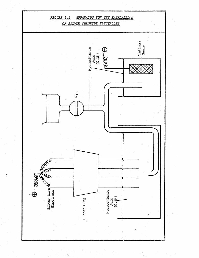
FIGURE 5.2 APPARATUS FOR THE PREPARATION
OF SILVER CHLORIDE ELECTRODES
i—I CDh u e :
o< o
D.
Oo
-pD
X)XI

5.3.3 MEASUREMENT OF EMF
The standard CERL data logging facility CDAPS [Computerised
Data Acquisition and Processing System] was used to construct EMF-
time graphs for each cell. CDAPS consists of .3 distinct modules.
[1] A high speed, high impedance digital voltmeter capable
of reading to ±0.0lmV.
[2] A multiplexer capable of connecting up to 800 channels
to the digital voltmeter.
[3] A control computer, which is also capable of use in an
off-line mode to allow data processing after acquisition.
r ' *
The input impedance of the system is greater, than lOMft which
prevents any ’loading’ of the cells and the multiplexer is capable
of sampling each cell at a maximum rate of once every minute.
Control of the system is from user teletypes'and video display
units distributed throughout the laboratories. These enable individual
channels to be switched on or off, and control to be exercised over
the rate of sampling. Teletypes produce a hard copy of results
whilst VDUs do not, so the latter were usually, used in conjunction
with digital cassette recorders to record results. The VDU-recorder
combination possessed a considerable advantage over the teletype in
that results could be fed back into the computer at a later date for
analysis.
The main advantage of the CDAPS system is that it frees the
user from time consuming measurements. Additionally, it is a 24
hour system so that runs can be performed overnight thus decreasing

the time necessary to acquire a given amount of data.
5.3.4 TEMPERATURE MEASUREMENT
Thermocoax Industrial Thermocouples were used for all
measurements. These are chrome-alumel devices designed to work
up to 900°C with an accuracy below 300° of ±2°C. The thermocouples
were always used in pairs, as shown in figure 5.3, one was immersed
in an ice/distilled water bath whilst the other was maintained at
the temperature to be measured.
CDAPS has the facility to.convert a thermocouple EMF directly
to a temperature (°C) using an internal program and this facility
was used at all times. The accuracy of the system was measured by
comparing the CDAPS result with the reading of a standard thermometer
at.50° intervals between 25° and 250°C (Table 5.1).
JTABLE 5.1
COMPARISON OF TEMPERATURES INDICATED BY A STANDARD THERMOMETER AND THE EXPERIMENTAL THERMOCOUPLE SYSTEM
,0 .Temperature ( C)
Thermometer Thermocouple
25 ' 2450 49
100 100150 151200 202250 . 252
The results were deemed acceptable, being within the
manufacturer’s specification for the thermocouples.

FIGURE 5.3 THERMOCOUPLE ARRANGEMENT FOR
TEMPERATURE MEASUREMENT
DO rHC Q.
0ZJrHCO DO E DO 0 O 4->
00i—ICD
Q.
83S3Bra2r*3$K.Tt~Z:
Dewar

Temperature measurements were made by a thermocouple sheathed
in stainless steel 18/8 attached to the autoclave body in addition
to the measurements which were made inside the autoclave.by exchang
ing one of the electrodes for a thermocouple. These internal
thermocouples were sheathed in INCONEL as early experiments showed
that, at temperatures greater than 175°C, the stainless steel sheaths
were subject to severe.attack by the experimental solutions. The
thermoelectric properties of the two types of thermocouple were
identical.
5.3.5 CELL DESIGN AND ASSEMBLY
The pyrex cells containing the test solutions were of simple
construction (figure 5.4), consisting of only two partsj the stem
and bulb. A high tolerance ground glass joint connected the two
and served to form a liquid junction between the reference and test
solutions.
Care.was taken to ensure that the stem and bulb matched pairs
were always kept together. The cells were made ready for use by
filling the bulb to -the top with test solution and firmly pushing
the stem into the bulb. This action trapped a very thin film of
test solution between the two faces of.the ground glass joint thus
forming a conductive path between the outside and inside of the cell
whilst preventing bulk transfer of liquid across the junction. Test
solution was then added.to the cell until the level was 15mm from
the top of the cell. At room temperature no detectable leakage
occurred from a filled cell over a period of 24 hours.

FIGURE 5.4 GLASS CELL
j( - ■ 1.0cm —
7 T \
8.0cm
\ l /
Stem
GroundGlassJoint
Bulb

5.3.6 LOW TEMPERATURE APPARATUS A W METHOD
A simple apparatus was constructed for use at temperatures
below 100°C and is shown in figure 5.5.
Daylight has been reported148 to cause problems with silver-
chloride electrodes so the outside of the white translucent PTFE
container was covered with black PVC insulating tape.
Four holes were drilled through the rubber bung to accept
the silver-chloride electrodes., namely, two for the reference
solutions and two for the test solutions.
A typical run proceeded as follows. Two cells were filled
with the test solution as described in section.5.3.5 and the outside
wiped dry. These were placed in the PTFE container and reference
solution carefully poured, in until the height of the reference
solution was the same as the height of the test solutions inside
the cells. This procedure minimised the pressure differential across
the liquid junction. Finally, the rubber bung was fitted into the
top of the container so that two electrodes entered the glass cells
and two the reference solution. The whole assembly was then placed
in the water bath to within 5mm of the top of the rubber bung. The
data logging system was connected and an EMF v time plot constructed.
The equilibrium EMF was then determined from the plot and the
equilibrium constant calculated.
5.3.7 HIGH TEMPERATURE APPARATUS AND METHOD
Measurements at: temperatures exceeding 100°C were carried out
in the apparatus shown.in figure 5.6. The autoclave which was of

FIGURE 5.5 LOU TEMPERATURE APPARATUS
Rubber BungElectrode
Test Solution
PTFE Pot
Reference SolutionTest Cell1


.standard design was constructed from mild steel except for the
bolts which were high tensile steel.
The high temperature electrodes consisted of a length of
solid silver wire, silver soldered to a longer length of PTFE-
insulated silver-plated copper wire of 2mm diameter, (figure 5.73.
Eight such electrodes were mounted in a pressure-tight joint at the4 ;
top of the autoclave (figure 5.83. The construction of the joint
is shown in figure 5.9.'. Two guide pieces held the PTFE-insulated
wires in position as they passed.through the zirconia . (ZrO^J loaded
PTFE 'KONAX' seal. Pressure was applied to the seal by the hollow
metal tube fA ’ which was pushed.down by. the screw cap 'B'. Thus
pressure caused the faces .of the seal to mate properly and also
reduced the size of the holes through which the electrodes passed
thus gripping them firmly in position and forming a pressure-tight
joint. Zirconia-loaded seals were used since normal PTFE seals
rapidly extruded past the sealing face * C* and eventually failed to
seal properly.
The electrodes were splayed out as shown in figure 5.8 to
take full advantage of the available space inside the autoclave.
The reference solution and test cells were located in a pyrex
beaker D at the bottom of the autoclave.
Pyrex cells identical to those used in the low temperature
apparatus were used (figure 5.53. Since eight electrodes were
available, four test cells, were used and four electrodes placed in
the reference solution.

E H
FIGURE 5.7 ELECTRODE CONSTRUCTION
Silver Plated Copper Wire
Solid Silver Wire
PTFE Insulation
Silver Solder
flDSfftnwrsai bi— eft>oauggaftgJgg: i

■— — --------------------------- — -----------------------------------------------------------------
FIGURE 5 .8 ELECTRODE ARRANGEMENT
AutoclaveHead
Electrodes
PyrexBeaker
ReferenceSolution
Test Solution
J

B B E B 1
FIGURE 5.9 KONAX SEAL
i b m i m
>
A D 0
Cap
Metal Guide Piece
Ceramic Guide Piece
O PTFE Plug Seal
Ceramic Guide Piece
\ /Body
A typical run proceeded as follows. All.the apparatus was
wiped dry except for the cells and beaker which were dried in an
oven. Four test cells were filled with, test solution, as described
in section 5.3.5; a gap of 10mm was left at the top of each cell.
The cells were placed.in the beaker and reference solution added
until the level outside the cells was the same as that within. The
beaker was carefully placed inside the autoclave body and the electrode
assembly placed.in position such that four electrodes entered the
cells and four the reference solution. Ten bolts, sequentially
tightened to ensure a good seal, were then screwed into the auto
clave body. The sealed autoclave was placed in a Perkin-Elmer fan
oven at the desired temperature and the electrodes and thermocouple
connected to the data logging system. This procedure was accomplished
in about 20 minutes. Generally the system was monitored for six
hours, at which time an EMF v time plot could be drawn and the
equilibrium EMF determined.
It was very difficult to determine whether any liquid had
been lost from the autoclave since a reflux system was set up inside
the autoclave on cooling. Hot vapour from the solution condensed
on the cooler sides of the autoclave and ran down between the auto
clave body and the pyrex beaker. Additionally, vapour condensed
on the electrode assembly and sometimes reacted with the mild steel
autoclave body, all of which made the determination of the volume
of liquid left in the autoclave unreliable. However, it was
estimated that more than 95% of the liquid was retained within the
autoclave, even at the highest temperatures.
All sealing faces and. bolt threads were coated with a suspension

of graphite in methylated spirit before use, to prevent jamming.
The only serious practical problem was corrosion of the mild
steel autoclave and its subsequent.effect on the efficiency of the
pressure seals. Extensive corrosion of the internal faces of the
autoclave was found in the form of a scale-like layer of surface
oxide. Occasionally some of this layer, fell into the pyrex beaker
although it was not possible to determine whether this occurred
during the experiment or after cooling and subsequent handling.
Despite being covered with a layer of graphite, corrosion of the
sealing faces did occur, and.frequent cleaning with oil and emery
cloth was necessary.
Due to the corrosion problem regrinding of-the sealing faces
for the mild steel autoclave became necessary and a nimonic steel
autoclave of identical design was used to finish the experimental
work. No corrosion, was evident with this device and the stability
of the EMF v time plots improved considerably. Typical results from
the two autoclaves are given in figures 5.10 and 5.11. It was felt
that the nimonic steel auto.clave gave better results because of
improved sealing of the pressure-tight joints.
5.3.8 DETERMINATION OF AVERAGE CELL EMF
When several reference electrodes were used, one was arbitrarily
chosen as the standard for that run and all other electrodes, includ
ing references, measured against it. Thus, if eight electrodes were
being used, three reference EMF and four test solution EMF would be
recorded.
The cell EMF were obtained by extrapolating to zero time the

BBBEE3 |
FIGURE 5.10 EMF v TIME PLOT FOR MILD STEEL AUTOCLAVE
LL
-P
H
-P
D.
Ooo□
CD
CM
□
CM
>ELLe ;uj
Time
(Hours)

FIGURE 5.11 EMF v TIME PLOT FOR NIMONIC STEEL AUTOCLAVE
CD
LU
CD
l-l
<
CL
CM
OCM
>eLLs:(U
RnrfCsaaBses reaaa*aara&?3'.?
Time
(Hours)

portions of the EMF v time plots which occurred after equilibration
as.shown in figures 5.10 and 5.11.
The three reference EMF were averaged to find the correction
which had to be applied to the test solution EMF to compensate for
imperfection in the arbitrarily chosen reference electrode. An
example is shown below:
Measured EMF (mV3 Electrode No. Type .
0.7 2vl Reference1.4 3vl Reference1.1 4vl Reference
10.5 5vl Test10.2 6vl Test11.1 7vl Test11.6 . . . 8vl ... Test
Arbitrary Reference Electrode = No. 1.
Average Reference EMF = CO.7+1.4+1.13/3 = l.lmV.
Thus corrected test EMF are 9.4mV
9. lmV
lO.OmV
10.5mV
Average = 9.8mV
5.4 RESULTS
Tables 5.2, 5.3 and 5.4 show the average measured EMF as
calculated above, the correction made for junction potential and
the values of K obtained at ionic strengths of 0.8, 1.3 and c2.3mol.Kg *.

TABLE 5.2a
RESULTS AT IONIC STRENGTH O.Smol.Kg"1
Temperaturet°C)
Measured EMF (mV) Correction (mV) for Junction
.... Potential.Low. Average . . High...
25 11.8 12.3 12.8 -1.050 14.3 14.3 14.3 -1.275 13.5 13.5 13.5 -1.3100 8.9 9.8 11.4 -1.5125 1.5 4.0 6.5 -1.8160 -5.5 -3.2 -1.5 -1.8185 -14.9 -10.9 -7.9 -1.9225 LDLDCM1 -24.8 -23.4 -2.2254 -41.1 i—10 •3-1 -38.2 -2.4
TABLE 5.2b
Temperature(°C)
log(Kc (from corrected EMF)
Low EMF Average EMF High EMF
25 1.54 1.53 1.5150 1.51 1.51 1.5175 1.55 1.55 1.55100 1.68 1.66 1.62125 1.83 . 1.79 1.74160 1.94 1.91 1.88185 2.07 2.02 1.97225 2 19 2.18 2.17254 2.35 2.34 2.32

TABLE 5.3a
RESULTS AT IONIC STRENGTH l.Smol.kg"1
Temperature(°C)
. Measured EMF (mV) Correction (mV) for Junction PotentialLow Average High
25 18.1 18.4 18.7 -0.350 16.6 17.0 17.4 -0.375 15.7 16.8 17.9 -0.4100 14.1 16.0 17.9 -0.5105 15.5 15.6 15.7 -0.5125 8.0 9.7 14.0 -0.6158 4.4 4.9 5.4 -0.7185 -2.7 -2.1 -1.6 -0.8212 -10.0 -9.0 -8.0 -0.9237 -24.2
.. ..... ...... — J
-19.5 -15.0 -1.0
TABLE 5.3b
Temperature(°C)
log (Kc (from corrected EMF)
Low EMF Average EMF High EMF
25 . 1.42 1.41 1.4050 1.42 1.40 1.3975 1.47 1.45 1.42100 1.54 1.50 • 1.45105 1.51 1.51 1.51125 1.68 1.65 1.56158 1.76 1.75 1.74185 1.88 1.87 1.86212 1.98 1.96 1.95237 2.15 2.09 2.04

TABLE 5.4a
RESULTS AT IONIC STRENGTH 2.3mol.kg-1
TemperatureVc)Measured EMF (mV3. . Correction (mV3
for Junction . . . .Potential ..Low Average High
25 10.1 10.2 10.4 -0.250 10.9 11.2 11.4 -0.275 11.4 11.6 11.8 -0.3
105 10.0- 11.5 13.0 -0.3127 6.5 8.2 10.0 -0.4158 5.0 6.2 8.3 -0.4181 4.7 6.2 7.7 -0.5215 -2.0 -1.0 0.0 -0.5
TABLE 5.4b
Temperature(°C3
log(Kc3 (from corrected EMF3
Low EMF Average EMF High EMF
25 1.56 1.56 1.5550 1.56 1.55 1.5575 1.57 1.57 1.56105 1.62 • 1.59 1.56127 1.70 1.67 1.63158 1.74 1.72 1.68181 . 1.75 1.72 1.70215 1.85 1.84 1.82
5.5 DISCUSSION
5.5.1 EXPERIMENTAL ERRORS
The primary sources of error in the calculated values of
were:

(1) Use of limiting equivalent ionic conductances
in the Henderson equation to calculate the liquid
junction potentials.
(2) Non-reproducibility of the liquid junction potentials.
(3) Extrapolation of the measured EMF to zero time.
(4) Uncertainties in the measured temperature due to
manufacturers’ tolerances on the thermocouples.
5.5.1.1 ERRORS DUE TO LIQUID JUNCTION POTENTIALS
These fall into two classes. The first is errors in the
theoretical junction potential, calculated from the Henderson
equation (5.12]. Values of the equivalent ionic conductance of
ions necessary to use equation (5.12) are not available at tempera
tures much above 50°C and in the absence of this data the limiting
equivalent ionic conductances were used to give an estimate of the
liquid junction potential.
The limiting equivalent conductance of several ions including
H+ and C£ have been measured to 400°C11*9. Plots of A vs T areoshown in figure 5.12. It is apparent that all the univalent ions
have similar temperature dependences. Aq for the perchlorate anion
however, has not been measured so an estimate of this quantity was
made from the Aq values,^ C£ from the equationxa f
,C£0+ _ ,C£0+ T oT n r ^f o 25 o -
25 o
2 +Similarly Jk values for Cd have not been measured so T oestimates were made from the 25° value of Aq and the temperature
dependence of the only divalent ion for which data is available

acne
FIGURE 5.12 LIMITING EQUIVALENT IONIC CONDUCTANCE OF SEVERAL IONS IN MATER AS A FUNCTION OF TEMPERATURE
1200 —
Conductance(ymho)
□H800
600
NaHSO400
200
3002001000
Temperature (°C)

2 -(SO^ ) using the equation
Hd2+ Hd,2 +
Inherent in this approach is the assumption that all ionic
conductances vary in the same way with changes in ionic strength.
it becomes so at the temperature's used in these experiments. However,
due to the paucity of data concerning electrolytes at.high ionic
of calculating the liquid junction potential suggests itself.
•The second source of error is non-reproducibility of the liquid
junction itself. Early experiments showed that the EMF deviations
of the electrodes were less than ± 0.2mV [section.5.3.2), however,
experimental deviations of as much as ± 3mV were noted between
supposedly identical cells. No correlation was found between
deviations and individual cells. Dirt or particulate matter in the
ground glass joints could account for this and strenuous efforts
were made to keep the joints clean, but the problem still persisted.
It was noted that the deviations decreased, with increasing temperature.
5.5.1.2 EXTRAPOLATION OF MEASURED EMF
The form of the EMF-time curves in the mild steel autoclave is
shown in figure 5.10. An internal thermocouple indicated the point
at which thermal equilibrium had been achieved. This was usually
accompanied by linearly-rising EMF at a rate of.l-4mV/hour. This
rise was initially, attributed to leakage of solution through the
liquid junction which could.also have caused the differences in EMF
This is not the case at 25°C and there is no reason to suppose that
strengths and at temperatures much removed .from 25°C no other method

between identical cells. However, when circumstances forced the
use of a nimonic steel autoclave,.the rates of increase of EMF fell
to between 0 and lmV per hour [figure 5.11). This suggests that
the mild steel autoclave had a small leak which was too small to
cause obvious loss of liquid, but large enough to show up as a con
centration change of the solution. Thermal syphoning between hotter
and cooler parts of the autoclave orloss of reactants due to corrosiontj ♦
could also have caused changes in EMF with time. A comparison of
identical runs performed in both autoclaves showed that, if the EMF
v time curves after attainment of thermal equilibrium were extrapolated
to zero time, identical results were obtained within the experimental
error.
For this reason all EMF were extrapolated.to zero time, before
averaging.
5.5.1.3 OTHER SOURCES OF ERROR
The following errors, have been ignored in the calculations as
they are much smaller than those introduced by the EMF deviations.
Ca3 Temperature uncertainties [± 2°C].
(b) Stoichiometric errors in solution concentration (<0.5%].
(c) Evaporation of water from the bulk of the solution to3
saturate the 50cm of air inside the autoclave. (0.5% at
125°C, 0.7% at 250°C].
5.5.2 CALCULATION OF THE ASSOCIATION CONSTANT OF CdCl*
Once the average cell EMF, corrected for junction potential,
at any temperature and ionic strength was calculated, the molal

concentration association constant could be found from equations
(5.5] and (5.10]. The following parameters were needed:
(1] Temperature C°C].
(2] Total cadmium concentration.
(3].Total, chloride concentration in reference solution.
(4] Total chloride concentration in test solution.
(5] Cell EMF.
The error in logtK^] was found by propogating the error in
EMF through equations.(5.5] and (5.10]. Below 100°C the average
error was ± 10% in log(K] and above 100°C the error was ± 20% in
log(K].
The percentage of ligand complexed (ML/L .] was. always between
30% and 50% thus giving a large difference between the total and
free chloride ion concentrations in the test cells. This reduced
the sensitivity of the calculations. to errors in the measured EMF.
5.5.3 INTERPRETATION OF RESULTS
5.5.3.1 COMPARISON OF RESULTS WITH PREVIOUS WORK
The results of.this investigation are shown in Tables 5.2,
5.3 and 5.4.
At all ionic strengths was found to increase mono.tonically
with increasing temperature. The log(Kc] v 1/T (°KJ curves at
ionic strengths of. 0.8M and 1.3M do not intersect, but the curve at
ionic strength 2.3M intersects once with both the 0.8M and 1.3M
curves.

Only one paper15® has been found concerning the determination
of the association constants of the aqueous cadmium.chloride system
at temperatures exceeding 50°C. Values of were reported at
temperatures between 0°C and 98°C in 0.066M calcium chloride by a
cation-exchange method.
Many examinations of the aqueous cadmium chloride system have<
been made at temperatures between 20 C and 35 C using a variety of
methods and in many different media. When constants for several
complexes have been determined simultaneously by previous workers
it was often found that the values were inter-related or that
neglect of one complex markedly altered the values of those remaining
and this situation is reflected in the lack of agreement between
previous determinations.
By far the most popular medium used tostudy the aqueous
cadmium chloride system is sodium perchlorate, but even in this
sub-section of the data,, considerable deviations exist between
determinations of (Table 5.5).
The determination of Reilly and Stokes152 eliminates many of
the assumptions made by previous workers. A cell without liquid
junction containing a cadmium-mercury amalgam electrode and a
silver-silver chloride electrode was used to determine the activity
coefficients of cadmium chloride-sodium chloride aqueous mixtures.
The treatment of.this data was essentially the determination of the
four stability constants and sixteen extended Debye-Huckel parameters
which best fitted the data. The stability constants were reported
to be well-defined in this system and to reach nearly constant values
early in the fitting procedure. The Debye-Huckel parameters were less

TABLE 5.5
LOGIK) FOE CADMIUM CHLORO-COMPLEXES AS A FUNCTION OF TONTG STRENGTH IN SODIUM PERCHLORATE AT 25°C
Medium . logCKj] log(K2) logCK3) . .log(K4) . . . Reference
->0 2.43 0.63 151-KD 1.93 0.43 -0.28 152->0 1.97 0.54 153+0 1.96 4> 154. .
0.5 1.37 0.43 155
0.76 1.46 0.38 0.13 156
1.0 1.20 0.6 1571.0 1.35 0.43 -0.36 155
2.0 1.38 0.76 -0.07 1582.0 1.36 0.28 0.12 1592.0 • 1.42 0.50 -0.16 1602.0 1.42 0.53 -0.16 155
3.0 1.50 0.81 1613.0 1.59 0.64 0.18 1623.0 1.46 0.78 0.07 1633.0 1.58 0.65 0.12 1643.0 1.54 0.66 0.09 1553.0 1.54 0.52 0.40 1653.0 1.39 0.79 0.21 166
•4.5 1.32 0.90 0.09 -0.45 167
well-defined but were reported to be reasonable.
It is instructive to quote from the closing paragraph of Reilley and
Stokes152 'The only conclusion possible after inspection of literature
values.is that the degree of complexing in the cadmium-chloride system
varies with the author and one may legitimately suspect all of the
thermodynamic data calculated from the variation of the stability
constants with temperature. It seems that most of the data on this
system are, at best, semi-quantitative.’

No reports of determinations in perchloric acid have been
found so no direct comparisons can be made with the present results.
5 . S . 3 . 2 Y M IA T W OF Kc WITHjrEMPEEATUEE
A van't Hoff plot (logCK^ v 1/Temperature (°K)) of the
results from Tables 5.2, 5.3 and 5.4 is shown in figure 5.13 from
which it can be seen that at every ionic strength the reaction has
a positive heat capacity and that the complex becomes more stable
as the temperature increases.
Reactions of this type:
2+ - + r r + x n x
are considerably effected by the dielectric constant (e) of the
solvent in which they take place due to the nett loss of charge
in solution as the reaction mixture equilibrates. As the di
electric constant of the solvent falls so the reaction as shown
will become more favoured and the experimental results are consistent
with this.
Two treatments of the results are possible depending on whether
ACp° is assumed to be temperature dependent or independent. Due to
the large error bands associated with the data points the simpler
temperature independent treatment has been adopted since no reliance
could be placed on the temperature dependance of the ACp° values
calculated in the former case.
The values of AH°, AS° and constant ACp° (Table 5.6) for this
system are not well defined as there are many sets of these para-

«ai
FIGURE 5.13 PLOT OF LOGiK ) v 1/T FOR CdC£+ AT c ------IONIC STRENGTHS OF 0.8, 1.3 AND 2.3mo1.K-1
C\l
CM
CM
I J
O
CO
MM
O*co
LDCM
COOi—i
X
o"CM
CM
b0D

meters'whidh adequately describe the experimental data within its
estimated error. The errors shown in Table 5.6 reflect this
situation.
TABLE 5.6ao
CALCULATED VALUES OF Aff°,AS?,ACp°AT IONIC STRENGTH 0.8mal.Kg_1
Temperature AH°(kJ.mol.-1)
AS°(J.mol-1deg._1)
ACp°(J.mol.-1deg. _1)
25 -□.5(2.0) 27(6)50 2.5(2.0) 37(6)75 5.5(2.0) 45(6)100 8.6(4.0) 54(12)125 11.6(4.0) 62(12) 29(5)160 15.8(4.0) 72(12)185 18.9(4.0) 79(12)225 23.7(4.0) 89(12)254 27.2(4.0) 96(12)
TABLE 5.6b
CALCULATED VALUES OF AH°, AS°, ACp° AT IONIC STRENGTH 1.3mol.kg_I
Temperature AH°(kJ.mol.-1)
AS°(J.mol.-1deg._1)
ACp°(J.mol.-1deg._1)
25 -1.5(2.0) 22(6)50 1.7(2.0) 32(6)75 4.8(2.0) 41(6)100 7.9(4.0) 50(12)105 8.6(4.0) 52(12)125 11.1(4.0) 58(12) 30(5)158 15.2(4.0) 68(12)185 18.6(4.0) 76(12)212 22.0(4.0) 83(12)237 25.1(4.0) 89(12)

TABLE 5.6c
CALCULATED VALUES OF Aff°, AS°, ACp° AT IONIC STRENGTH 2.3mol.Kg"1
Temperature AH°(KJ.mol.-13
AS°(J.mol.”1deg.“1)
ACp° (J.mol.-1deg.-13
25 -0.9(2.03 26(6350 0.6(2.03 31(6 375 2.2(2.03 36(63105 4.1(4.03 41(123127 5.5(4.03 45(12) ■ 15(5)158 7.4(4.03 50(12)181 8.8(4.03 53(12)215 11.0(4.03 57(12) .....
Plots of log(Kc) vs 1/eT for similar systems168 have been
shown to be linear at temperatures exceeding 100°C. This has been
explained by postulating that the free energy of association is made
up of two components.
AG = AG° + AG° o e Chem
AGg is an electrostatic, component due to the creation of a
modified electric field around the ions and AG° is a chemicalChemcomponent due to the formation of the new complex.
Born’s equation168j169 can be used to estimate AG°
2AG° -e er
Where e is the charge on the electron
e is the dielectric constant of the medium
r is given by — = i(— — + — 3 the mean ionic radius& r 2 r2+ r_N is Avogadro’s number

Ne2Thus logCK 3 = logCK 3 , - ( -— - 3a c Chem RreT
(R is the gas constant.3
The chemical contribution to the free energy of the reaction,
i.e. that typified by an isoelectric reaction, would be expected
to vary linearly with 1/T, i.e. constant AhLL . However, asChemFigure 5.13 shows, a plot of logCK. 3 vs 1/T is not linear indicating
that the first term in the above equation is not dominant. A plot
of logCK^) vs 1/eT (figure 5.143 however is much more linear
suggesting the dominance at higher temperatures of the electrostatic
component of the equation. r
In the absence of dielectric constant data for perchloric
acid solutions at high temperatures, the dielectric constants of pure
water23'187 have been used.instead and this constitutes a major
source of error in Figure 5.14.
5.5.3.3 VARIATION OF K WITH IONIC STRENGTH------------- C ------ !------------One striking feature of the log(Kc3 vs 1/T plots (figure 5.133
is the effect of temperature on the relative ordering of the
values at different ionic strengths. At 25°C the order is 2.314 >
0.8M > 1.3M whilst at 10(3°C it is 0.8M > 2.3H > 1.314 and at 225°C is
0.8M > 1.314 > 2.314.
This ’crossover' could be caused by the changing with temperature
of the effect of ionic strength upon:
(13 The dielectric constant of the bulk medium.
(23 The activity of water (affecting solvation3.

FIGURE 5.14 PLOT OF LOG IK) v 1/eT FOR CdCZAT IONIC STRENGTHS OF 0.8, 1.3 AND 2.3mol.KG-1
CO
CO HCOaCM
HCOMCO
CO
CO
CM CO COI—I I—I I—I
LD • O
Cl3/T
)

(3) Activity coefficients of the reacting species.
Dissolved electrolytes such as hydrogen chloride have been
shown to reduce the dielectric constant qf water according to the
equation170.
e = e + 26c o
£ is the dielectric constant of the medium
£q is the dielectric constant, of pure water
c is the molal concentration
6 is a constant for each electrolyte Cl ^ 23
.6 = -10kg.mol. for HC£ at 25°C
Thus at 25°C and a concentration of 2 molal the dielectric
constant of a hydrochloric acid solution is 36 compared with 76 for
pure water. As noted in section 5.5.3.2 a.decrease in dielectric
constant of the .bulk medium will cause an increase in K forcequation (5.13 however, the linear dependence of e on c prevents
the formation of a crossover, thus eliminating factor 2 as a possible
explanation.
Equations (5.13) and (5.14) show that Kc will depend on the
activity of water, to an extent determined by the change in solvation
during the reaction.
M2+(Aq) + X"(Aq) ^ MX+(Aq) + nhLO (5.13)£.
.,(MX)(H20)NK., = — r:---'— t-ttt— ( ) denotes activityth (M).(X) .
■_ [MX] YMX N „ „ N renal. a.. „ = K ..r.a., „ [5.14)[M] [X] • y^.Yx ' H20 c H20

If the activity coefficient expression T remains constant,
then a decrease in the activity of water will cause an increase in
Kc» Since the activity of water decreases171.with increasing ionic
strength, K would be expected to rise correspondingly. There is no creason to suspect that the activity of water as a function of ionic
ostrength will change direction at higher temperatures which may
eliminate factor 3 as a source of the 'crossover'.
It has been shown for many mixtures172 including 173 HC£-BaC£
to 175°C that the mean activity coefficient of the bulk electrolyte
greatly affects the mean activity coefficient of other ionic species
present.in solution. Thus if the ionic strength dependence of the •
activity coefficients of the bulk electrolyte (perchloric acid)
changed with temperature a .'crossover' could be generated.
areNo data %£> available concerning the activity coefficient of
perchloric acid as a function of ionic strength and temperature.
However, the mean activity coefficient of hydrochloric acid as a
function of ionic -strength and temperature has been measured174 and
this will be used as a model for perchloric acid since the two acids
show similar ionic strength dependencies at 25QC.
Equations (5.15) and (5.16) show the relationship between Kc
and the activity coefficient term for equation (5.1).
K„ = K .T " (5.15)th c
“ . K K .— .(5.16)° TCd2+Y - * C YCd2+
Thus if y ,2+ decreases K must also decrease and vice versa, ' Cd c

^Cd^+ depend upon the mean activity coefficient of the
bulk electrolyte and will be expected to follow changes in it.
Thus is expected to follow the mean activity coefficient of the
bulk electrolyte also.
The mean activity coefficient of hydrochloric acid as a -
function of ionic.strength and temperature is given in figure 5.15
from the equations in reference 174. It is apparent' that, as the
temperature increases, so the minimum in y moves to higher ionic
strengths and the relative ordering of y with ionic strength changes
from 2.014 ■> 1.014 > 0.514 at 25°C to 0.514 > 1.014 > 2.014 at 200°C.
Since K is expected to follow these trends, a 'crossover’ csituation is produced in which the relative order of as a function
of ionic strength changes with temperature.
It is concluded that the 'crossover' exhibited in figure 5.13
is due to changes in the ionic strength dependence of the mean
activity coefficient of perchloric acid with changing temperature.
Should metal-halide complexes be extensively studied in perchloric
acid media at high temperature, it would be an interesting test of
the validity of this conclusion.
5.5 EFFECT OF OTHER CADMIUM CHL0R0-COMPLEXES
The experimental conditions were designed to reduce the formation+of complexes higher than.CdCJt by maintaining an excess of cadmium
ion over chloride ion. There were, however, two constraints on the
extent to which this could be done, the first was imposed by a desire
to keep the reference and test solutions of similar composition to

FIGURE 5.15 MEAN ACTIVITY COEFFICIENT OF HYDROCHLORIC ACID AS A FUNCTION OF IONIC STRENGTH AND TEMPERATURE
u CJ u uu U CJ in o in ;
o O O CM m r \LD □ □ i—i ■—i —CM CD cn
oCM
1o
>i—i •P
•H -p> c•H 0■P •HO O
< •H
CH-H-
CO 0m G
z : CJ
Ionic
Strength
(Mol.Kg

reduce junction potentials. The second arose from the sensitivity
of the calculations to deviations in EMF when the ratio of total
cadmium concentration to total chloride concentration was high. A
ratio of 2:1 was chosen as the best compromise between these
factors.
At 25°C is about 5kg.mcl. (Table 5.5). If this is
neglected, when calculating K^, then the resultant value will be
about 8% high. Chloro-complexes higher than the second do not
contribute significantly at the cadmium:chloride ratios used.
Experiments to determine at 25° were unsuccessful because
of the'non-reproducibility of liquid junction potentials and the
consequent, uncertainty in the free chloride ion concentration.
Since .the overall experimental error was so high the effects of
were neglected at all temperatures.
5.6 CONCLUSIONS
This experimental technique and subsequent analysis suffer
three major disadvantages:
(1) The ionic strength is too high for
practically useful results.
(2) The errors from nonr-reproducibility
of the liquid junction are large.
(3) The extreme approximations necessary to
apply the Henderson equation at high
temperature render correction for the
liquid junction potential, at best, uncertain.

Points 2 and .3 could be evaded by using a system with no liquid
junction. The standard EMF of the hydrogen-platinium, silver chloride-
silver cell has already been measured to 250°llf5 with an uncertainty
of ± 0.2mV.
H2-PtJ HC&| AgC£.Ag
This is more than an order of magnitude better than the EMF deviations
of.the present experiments and would give information on the activity
of the chloride ion.
Alternatively, a high temperature mercury amalgam electrode
could be constructed and used in a two or three electrode arrangement
with hydrogen and silver-chloride electrodes. The activities of both
chloride and metal, ion could.then be.determined directly and an
analysis similar to that of Reilly and Stokes152 performed.
The use of a mild steel autoclave undoubtedly introduced errors
due to leakage and corrosion which were absent when a nimonic steel
autoclave was used. Nimonic steel is, therefore, highly recommended
for use in this type of experiment.
The sensitivity of the calculations to errors in EMF imposed
constraints upon the reagent concentrations that could be used which
in turn did not allow the use of conditions which precluded the
formation of the second complex. If the deviations in EMF could be
reduced then:more precise results could be obtained under more+favourable conditions and less.stable complexes such as CuC£ and
+ZnC£ could be studied.

The Central Electricity Generating Board is primarily
interested in reactions which occur in the relatively dilute
conditions of power station boilers. For this reason, thermodynamic
constants would be of more value than those which prevail at high
ionic strengths and efforts should be directed towards developing
experimental techniques which give access to thermodynamic constants
such as those due to Reilly and Stokes152. Whilst a conductimetric<>
method might appear to be advantageous,. hydrolysis of metal ion
species may occur, at the prevailing ionic concentrations which
would be necessarily low and would become a more severe problem as
the temperature was raised.

CHAPTER 6
THE ASSOCIATION CONSTANT OF THE FIRST CHLORO-COPPER COMPLEX
AS A FUNCTION OF TEMPERATURE

6.1 INTRODUCTION
The study of chloro-complexes is of interest for reasons
discussed in Chapter 5. Due to inherent drawbacks the experimental
procedure described in that chapter could not be applied to very ’•
weak complexes such as the first chloro-copper (II) complex (K ^
1.7, I = 1 .OM) and alternative methods of study were sought.
■Spectrophotometric methods have been used by several workers
since some transition metal chloro-complexes exhibit UV-visible
spectra which are significantly different from those exhibited by
the corresponding free metal ions.
Many authors have performed studies at constant ionic strength;
the two most popular electrolytes being perchloric acid and sodium
perchlorate. However, it can be argued, at ionic strengths less than
unity, that the activity coefficients of the reacting species, in
equimolal mixtures, were not. constant with changing solution com
position since the background electrolytes were not present in over
whelming concentration. This criticism can be applied to many
studies176* 177* 179> *80 Weak complexes and has been discussed by
Matheson1 8 1 although a different approach has been adopted by Libus178.
In this technique1 7 8 magnesium perchlorate is used as the
background electrolyte, for the study of divalent transition metal
halo-complexes. It is proposed that equimolal.mixtures of. transition
metal perchlorates and magnesium perchlorate may be considered as
constant ionic strength media. This concept is.supported by measure
ments of the activity coefficients of the components of mixtures of
transition metal perchlorates which show no composition dependence1 7 0 ' 1 8 2

within experimental error. Mixtures of copper (II) and magnesium
(II) perchlorates display the same behaviour up to lmol.kg \
while at higher concentrations their osmotic and activity coefficients
are detectably but only slightly lower than the values obtained for
the transition metal, ion mixtures. Activity coefficients in this
system will undoubtedly be more nearly constant than when a mono
valent cation perchlorate, such as perchloric acid or sodium per-1'
chlorate, is used to control.the ionic strength.
The studies in Chapter 5 of the association.constant of the
first chloro-cadmium complex as a function of temperature and ionic
strength revealed a ’crossover' effect in which the relative order
of stabilities of the complex at a series of ionic strengths was
temperature dependent. This was attributed to the ionic strength
and temperature dependence of the activity coefficient of perchloric
acid which.was used as the background electrolyte in those experiments.
In order to verify the conclusions.described in that chapter, it was
desirable to measure the association constant of another transition
metal chloride in perchloric acid as a function of temperature and
ionic strength, preferably by a different technique to that described
in Chapter 5.
It is clear from the above constraints that magnesium perchlorate
with its attendant advantages as described.by Libus1 7 8 cannot be used
as., background electrolyte and so the experiments described in this
chapter are open to . the same criticisms concerning constancy of ionic
strength in equimolal mixtures as the majority of previous work on
these systems. An additional. factor precluding the use of magnesium
perchlorate in these experiments was the unknown behaviour of the'
association constants of the magnesium chloro-complexes as a function

of temperature.
The first chloro-copper (II) complex was chosen as the subject
of a spectrophotometric' investigation in which the temperature and
ionic strength dependence of its association constant in perchloric
acid were measured. This system has been the subject of a great
deal of work1 7 6 - 1 8 0 , 1 8 3 using many experimental techniques, although4 '
little agreement can be .found between the results.obtained by different
workers. This is mainly, due to the wide variety of background
electrolytes used and the necessarily arbitrary choice of the number
of significant complexes present under the prevailing experimental
conditions.
The method of analysis adopted here was that used by McConnel
and Davidson1 7 8 and Libus1 7 8 which involved the use of solutions
containing a small concentration of chloride ion C'v 0.005M) and a
relatively large concentration K 0.2M] of copper (II) :\ion. The
concentration of copper (II) was varied at a fixed chloride concen
tration and the resulting spectral changes noted from which the
association constant.was calculated.
Under these conditions, calculations based on association
constants for the successive copper complexes given in reference 183
indicated that only the first complex would be formed in significant
concentrations.
Carlsson and Wettermark1 7 7 have used a computerised least
squares method to calculate extinction coefficients and association
constants for the first two. copper (II) chloro-complexes although the

results calculated depend significantly on the form of the equation
used and it is not clear whether this method provides more reliable
results than graphical methods.
6.2 THEORY
6.2.1 ASSUMPTIONS
The method used by McConnel and Davidson1 7 6 and Libus1 7 8 was
employed. Since so little complex is formed relative to the con
centration of free metal ion, it is assumed that the free metal
ion concentration may be taken to be the total.metal ion concen
tration. In these experiments, the free metal ion concentration
was 99.2% - 99.4% of the total met-al ion concentration.
An iterative loop could have been employed to compensate for
the difference between the total and free metal ion concentrations
but early work indicated that the overall experimental error was
much larger than the corrections obtained by the iterative procedure
and this correction was.not applied.
6.2.2 EQUATIONS
The equilibrium being studied was as follows
n 2 + + L~ ML + (6.13
where M = Cu and L = C£.
Two mass balance equations pertain to this system
My = Mp + ML
(6,23

M^ = total metal ion concentration
L.j. = total ligand concentration
Mp = free metal ion concentration
Lp = free ligand concentration
ML = complex ion concentration
Now M_ MtF ^ T f,
and ML = K M._L_ where K is the concentration association constant c F F • cfrom equation (6 .1 ).
Thus, from equation (6.2),
Now the absorbance at a particular wavelength is made up of
two components; that due to the free metal ion and that due to the
complex. Thus
A = absorbance at a particular wavelength
e = extinction coefficient of the free metal ion oe = extinction coefficient of the complex ion
£ = path length = 1 cm
L -------F 'v 1 + K M.c T(6.3)
A = e M._£ + eML£ o F (6.4)
Equation (6.4) can now be expanded, taking £ = l.Qcm, to give

A = e M_ = absorbance of a solution of metal ions of concentration o o TM-j. in the absence of ligand.
eK M LA ft Ao Y+k mtc T
. cK M L(1 + K M ) <v T Y --. c T 'v (A-A ) o
Lt (1+K Mt) T c TCA-A ) ^ eK Mt o c T
LT 1 1 ro^ —7/— ivi— + — (6.5)(A-A ) 'v eK M_ e o c T
This equation is of the form y =f mx + c in which A-Aq and M^LT 1are the variables. Thus a plot of 7 -y y y against — should give a
LA A J Pi—
1 G 1straight line of slope — and intercept — from which e and K may£r\ C CCbe calculated.
6.2.3 USE OF SQUAD
The computer program SQUAD (Chapter 2) was not used to
calculate the association constant in this system due to the near
linear relationship between the absorbance and metal ion concentration
This gave rise to large uncertainties in the values calculated by
SQUAD and sometimes resulted.in divergence.

6.3 EXPERIMENTAL
6.3.1 PJJRITY, PREPARATION AND STANDARDISATION OF REAGENTS
6 .3.1.1 COPPER PERCHLORATE
A copper perchlorate stock solution (^ l.OM) was prepared
from copper (II) oxide (80.04g, BDH, 99% pure) dissolved, on heating
in a mixture of perchloric acid'(323g, BDH, AnalaR SG = 1.70) and3de-ionised water (2 0 0 cm ) which was finally made up to 1 . 0 litre.
The resulting copper (II) perchlorate solution was analysed
for copper by EDTA titration using fast sulphon black F indicator
according .to Vogel1 8 *1 and agreed to. within < 1% of the value cal
culated from the weight of oxide used.
The acid concentration of the solution was determined by pH
titration against standard sodium hydroxide. A plot of pH against
concentration of sodium hydroxide added was constructed and it was
found .that hydrolysis of the copper buffered the solution at about
pH 4 at the end of titration. The volume of alkali needed for
neutralisation of the acid was found by extrapolating the steepest
part of the pH plot to pH 7 and reading off the required volume of
alkali. The concentration of residual acid calculated in this way
differed by < 1 % compared with that calculated.from the initial
reagent concentrations.
6 .3.1.2 ACIDS A W ALKALIS
Sodium hydroxide (0.1M), hydrochloric acid (0.1M) and per
chloric acid (5.014) were prepared and standardised in the manner
described in section 4.3.4.8 .

6.3.2 ABSORBANCE MEASUREMENTS
The use of glassware and. optical cells is described in
section 4.3.5 and the use of the low and high temperature spectro
meters is described in sections 4.3.1 and 4.3.2.
6.3.3 METHOD" t
Two series of solutions, X and Y, corresponding to Aq and A
in equation (6.5) were prepared from stock solutions of copper
perchlorate, perchloric and hydrochloric acids. The X and Y solutions
were identical except that the X solutions contained no hydrochloric
acid. The compositions used are given in Table 6.1.
TABLE 6 . 1
EXPERIMENTAL COPPER (IT) AND CHLORIDE ION CONCENTRATIONS
SolutionCopper (II)
Concentration (mol. )
Chloride Ion Concentration
(mol.A-1)
1 X 0 . 0 2 - . .
1 Y 0 . 0 2 0.0052 X 0.05 -2 Y 0.05 0.0053 X 0 . 1 0 -' 3 Y 0 . 1 0 0.0054 X 0.154 Y 0.15 0.0055 X 0 . 2 0 -5 Y 0 . 2 0 0.0056 X 0.25 -6 Y 0.25 0.005
To each solution was. added sufficient perchloric acid to
achieve the desired constaht ionic strength.
The absorbance of each solution was then measured^at 265nm, .
270nm, 280nm and 290nm. The difference spectra Y minus.. X could hot

be measured directly because (a) the SP3000 spectrometer used at
temperatures less than 90°C could not function correctly with a
reference absorbance greater than 0 .2 .
Cb) the SP1800 high temperature
spectrometer had no facility for placing a heated sample in the
reference beam.
The values of the difference spectra at a particular wave
length were then calculated by subtracting the X absorbances from
the Y absorbances. These differences corresponded to the term
(A-A ) in equation (6.5) and the values of and e at any wave
length were found by plotting ')' agains‘t pf" •o T
The intercept gives and the slope —I— r-E K £l— _T c T
Thus e = r— -— -r—;—Intercept.
„ _ Interceptc Slope
This process was then repeated for the remaining wavelengths
and the mean and standard deviation calculated.
6.4 RESULTS
6.4.1 CALCULATED VALUES OF ASSOCIATION CONSTANT
AND EXTINCTION COEFFICIENT
K has the units Jl.mol 1
■ -1 -1 e has the units £.mol cm

IONIC STRENGTH = 1.0M PERCHLORIC ACID TEMPERATURE = 24°?
A e eK K logCK)
265 426 720 1.69 0.23270 321 526 1.64 0 . 2 1
280 148 258 1.75 0.24290 93 124 1.34 0.13
IONIC STRENGTH = 1.0M PERCHLORIC ACID TEMPERATURE = 49°C
A e eK K log(K).
265 669 1 2 2 0 1.82 0.26270 471 935 1.98 0.30280 242 467 1.93 0.29290 108 . 240 2 . 2 2 .0.35
IONIC STRENGTH =1.0M PERCHLORIC ACID TEMPERATURE = 75°C
X c eK K . logCK)
265 894 1958 2.19 0.34270 604 1413 2.34 0.37280 358 877 2.45 0.39290 142 264 1 . 8 6 0.27
IONIC STRENGTH = 1 . 0 M PERCHLORIC ACID TEMPERATURE = 100°C
X e eK K log(K)
265 _ (a)- - -
270 - - - -280 482 1330 2.76 0.44290 2 1 0 . . . .709 .3.38.. . .0.53. .
(a)Absorbance values at these wavelengths were beyond the maximum measurable by the SP1800 [A = 2.00).

■ 6.i|.2 SUMMARY OF RESULTS
Ionic Strength = l.Omol.A \ perchloric acid.
1
uo1— K (Amo-1. ■*■) . c log(K ). c24 1.70 0.23(8)49 1.91 0.28(8)75 2.34 0.37(8)
1 0 0 3.16 0.50(8).
6.4.3 EXTINCTION COEFFICIENTS
TemperatureExtinction Coeff. of Cu(H_0)^+ at
Z b265nm 270nm 280nm 290nm
25 0.96 0.47 0.15 0.0650 1.51 0.73 0 . 2 2 0.0875 2.34 1 . 1 0 0.27 0 . 1 0
1 0 0 - - 0.33 0 . 1 1
TemperatureExtinction Coeff. of CuCMH^O)*' at
2 b265nm 270nm 280nm 290nm
25 426 321 148 9350 669 471 242 10875 894 604 358 142
1 0 0 - - 482 2 1 0
6.5 DISCUSSION
6.5.1 ERRORS IN EXTINCTION COEFFICIENT AND ASSOCIATION CONSTANT
The method of calculating the extinction coefficient and
association constant for the first chloro-copper (II) complex makes
use of equation (6.5) in a re-arranged form (equation (6 .6 )).

1- 1 1(A-A ) “ LTeK M_ + elo T c T T
(6.6)
A typical set of data and corresponding plot are shown in
Tables 6.2 and 6.3 and figure 6.1.
_ _ nTemperature = 25.0 C L_ = 5.00x10 M HCJt
Ionic Strength = 1.0M made*up with perchloric acid
• TABLE 6.2
Data Used to Construct Figure 6.1
mt
265nm 270nm
A A0
A . A. . . □0 . 0 2 0.091 0 . 0 2 1 0.062 0 . 0 1 1
0.05 0.214 0.050 0.145 0.0240 . 1 0 0.407 0.099 0.274 0.0490.15 0.579 0.144 0.389 0.0730 . 2 0 0.735 . 0.191 0.493 0.0950.25 .0 . 8 8 8 0.238 0.592 0.118
TABLE 6.3
Data Used to Construct Figure 6.1
"t i/mt265nm 270nm
A-A0
1/(A-A ) 0
A-A□ 1/(A-A ) □0 . 0 2 50.0 0.070 14.29 0.051 19.610.05 2 0 . 0 0; 164 6 . 1 0 0 . 1 2 1 8.260 . 1 0 1 0 . 0 0.308 3.25 0.225 4.440.15 6.7 0.435 2.30 0.316 3.160 . 2 0 5.0 0.544 1.84 0.398 2.510.25 4.0 0.650 1.54 0.478 2.09
It is clear from figure 6.1 that, due to the use of the 1/M
term as the X co-ordinate, the slope is determined largely by the
solutions of low metal ion concentration. The metal ion concen
trations are Known to be better- than ±1% and this source of error

FIGURE 6.1 A TYPICAL PLOT USED IN THE DETERMINATION OF THE ASSOCIATION CONSTANT OF CuCZ+
20.0 270NM
1/(A-A ) o
15.0
/ 2B5NM
10.0
5025D
i / n T

will be neglected in the following discussions as it is much smaller
than the errors in the Y co-ordinate.
The Y co-ordinate is 1/(A-A 3. Both A and A are absorbanceso odetermined to ± 0 . 0 0 2 absorbance units, thus the uncertainty in the
quantity (A-A ) will be ± 0.004 absorbance units and the corresponding
uncertainties in 1/(A-A 3 are shown in figure 6.1. The error in
slope brought about by the uncertainties in 1/(A-A 3 is ± 7% of the
mean value whilst the error in intercept is ± 16% of the mean value.
The high value of error for the intercept is bought about by virtue
of its close proximity to the X axis. The extinction coefficient,
which is calculated from the intercept, is thus known to ± 16%
and eK to ± 7%. The errors, however, accumulate in K whichc ccan only be determined to ± 23%.
It is clear from figure 6 . 1 that the uncertainty in ,1/(A-A 3
decreases with increasing metal ion concentration and it would thus
appear desirable to only use solutions of high metal ion concentrations.
However, at high metal ion concentrations,, the assumptions made
concerning constancy of ionic strength in equimolar solutions become
questionable and from this point of view the use of solutions of
low metal.ion concentration is preferred. Thus solutions of low
metal ion concentration are suspect due to the relatively large un
certainties in 1/(A-A 3 and solutions of high metal ion concentration
are.suspect from ionic strength considerations. .
This situation can be improved by measuring the difference
A-Aq in one stage rather than two by utilising both sample and
reference beams of the spectrometer simultaneously, in which case

the uncertainty in A-Aq would be ± 0 . 0 0 2 absorbance units rather
than ± 0.004 absorbance units and the uncertainty in K^ would be
reduced to ± 12%. This was not possible in these experiments due
to limitations in the design of the available equipment which were
detailed in section 6.3.3.o
The situation cannot be improved by selecting a wavelength at
which e is smaller than the values encountered at 265 and 270nm
because, although the intercept will increase in value, the slope
will become steeper and the uncertainty in the intercept will remain
almost the same. A further disadvantage of small extinction
coefficients is the need to use more concentrated solutions with
their corresponding ionic strength considerations. Higher
extinction coefficients will reduce the slope allowing a more
precise determination, of the intercept which will, however, have
reduced in value which, in turn, will increase the uncertainty.
This simple analysis shows a marginal preference in favour of larger
extinction.coefficients although there is a limit to which the value
can be increased due to the consequent proximity to the X axis.
As K decreases so e becomes better defined although eK c cbecomes less well defined and.conversely, as Kc increases, e becomes
less well defined and eK becomes better defined. As K increasesc cto values greater than 5£„mol * the near linear.relationship between
(A-Aq) and disappears to be replaced by a curved relationship
(Figure 6.2) which is amenable to analysis by. SQUAD.. It is not
surprising that the errors generated by use of equation (6.5) are
so large since the analysis is solely dependent on the deviations
of the A-Aq against plot from linearity. It can only be concluded

FIGURE 6.2 EFFECT OF K ON A PLOT OF ABSORBANCE------------------------------- c— -------------------------------------------------------------
v TOTAL METAL ION CONCENTRATION (I SOLUTIONS)
o ai—i in
r \ co • O
GJ
COCO
CDOctoJDU□tnX]<
inCM
CD
aCM
CD
ini—iCD
CDi—i
mOCD
CD a
cQ■H4-5COu4-5CCDOcoCD
c0M 1-----Ito4-50)
i-H(04-5Oh-

that great care must be taken when using this method of analysis
to avoid underestimating the errors involved.
6.5.2 EXPERIMENTAL PROBLEMS
Few problems were experienced whenwusing 1cm silica optical
cells in the SP3000 spectrometer at temperatures less than 9D°CJ
however, the high temperature optical- cells used with the SP1800o*'at temperatures greater than 90 C gave considerable trouble.
Absorbance:readings were found to increase rapidly with time at 125°C
such that accurate absorbance measurements were impossible.
The experimental solution,, in this case perchloric acid
(0.75-.1.OOM) containing amounts of copper (II] chloride ion and +CuCit ion, was in contact with teflon and sapphire only. Hence
as no absorbance drift was found when using silica cells in the
SP3000 at 90°C it was concluded that the teflon or sapphire and
perchloric acid were interacting to give a soluble product which
absorbed in the wavelength range 260-290nm.
To test this conclusion perchloric acid (5.OH] was heated in
the cell for 12 hours at 150°C and the absorbance monitored.oFinally, the spectrum of the solution was measured at 25 C on an
SP8000 scanning UV-visible spectrometer. The absorbance-time plot
is shown in figure 6.3 and the spectra of the solution (dilution x2]
before and after heating are shown in figure 6.4.
Figure 6.3 shows that there was a continuous increase in
absorbance with time after an initial warm up period and figure 6.4
shows that the product exhibits maximum absorbance at 236nm.

FIGURE 6.3 ABSORBANCE OF 5M PERCHLORIC ACID ' AT 150°C AS A FUNCTION OF TIME
TJi—i
i—i
c_>
X]
IX)
CLDl
O
O
XJ

FIGURE 6.4 SPECTRUM OF 5M PERCHLORIC ACID AFTER 1 2 HOURSAT 150 C IN HIGH TEMPERATURE CELL. DILUTION C2x)
incot—fn E O 2 CD □ JO o < CO
aCO
-p
COCO ui
CM
CD
JO
Wavelength
(nm]

No signs of attack were found on the highly polished windows
and so it was concluded that perchloric acid was attacking the teflon.
No absorbance increase with time was noted.when sodium perchlorate
(5.ON) was heated in place of perchloric acid.
The object of these studies was to investigate the cross-over
effect, noted in Chapter 5, in the copper (II) chloride system.
However, the cross-over effect manifested ifself only above 100°C
and so, in view of the experimental difficulties, it is not possible
to comment on the cross-over effect based on the data obtained or
obtainable with the current equipment. This study was therefore
concluded without measuring the association.constant at other ionic
strengths.
As with the cadmium experiments, this investigation was
exploratory. As far as spectrophotometric experiments are concerned,
perchloric acid is an unsuitable medium so that direct comparison
with the results from concentration cell measurements are unlikely
to be obtained. However, the method is of some use in the deter
mination of low values of equilibrium constant in the chloride
system but a rigorous examination would require the collection of
a large amount of data in order to reduce uncertainties in the
values.
/
6.5.3 RESULTS AT IONIC STRENGTH l.Omol. i~1
Comparison with previous, work is limited to 25°C and Table 6.4
shows a typical selection of previous determinations.

TABLE 6.4
IonicMedium Method e
272nm K eK 272nm. Reference
1.0HC£04 Spectrophotometric 186 2.3 428 1771.0HC£04 Spectrophotometric 320 1.3 416 1761.0HC£ Spectrophotometric 1478 0.34 503 1850.691HC£04 Cation Exchange - 9.6 - 1801.0MgC£04 Spectrophotometric 1115 0.44 455 1781.0NaC£04 Kinetic ■ - 1.41 - 1792.0l\laC£04 Spectrophotometric 394 1 . 2 2 481 186
0 Spectrophotometric 1478 1 . 1 1 1640 1850 Spectrophotometric 1115 1.63 1817 178
1.0HC£04 Spectrophotometric 276 1.70 470 This Work
The values obtained in this work are in reasonable agreement
with the rather wide range of values found by other workers. In
particular, the values of e and K found in this work fall betweencthe values found by McConnel and Davidson1 7 6 and Carlsson and
Wettermark1 7 7 which were both obtained in l.GM perchloric acid,
but these experiments cast no light on the high values of extinction
coefficient found by Libus1 7 8 and Nasanen185. The van't Hoff plot
(logCK^) v 1/T C°KD 3 from the values given in section 6.4.2 is shown
in figure 6.5. In view of the arguments put forward in Chapter 5
analysis has been made in terms of a temperature, invariant value of
ACp°. The plot is of the expected form although the heat capacity
(150(40]J.deg. ^mol. is about five times larger than that found
for [CdC£] (30J.deg. ^mol. *]. Values of AH° and AS° at 25° are
given in Table 6.5.

“ IFIGURE 6.5 PLOT OF LOGiK ) v 1/T FOR CuCZ AT---------- o------
AN IONIC STRENGTH OF l.Omol.Jt - 1
Log (K )
0.6
0.4
0.2
0.0 __
2.5 3.0 3.5
1/T C I O
*r. wnwmm n — argggg-jarffl

TABLE 6.5
ENTHALPY AND ENTROPY OF ASSOCIATION FOR CttCl* AT 25°C
AH° (kJ.mol.-1) . AS°.(J.deg.. mol.-1).. Reference.
1.5(7) 9.2(5) This Work
Experiments by other workers over large temperature ranges
have not been made and no meaningful values of AH°, AS° and ACp°
can be found for comparison with this work.

• REFERENCES
1. D. Turner, (Conference Paper B.ll, 'High Temperature, High Pressure Electrochemistry in Aqueous Solutions'j National Association.of Corrosion Engineers, USA, 1975).
2. D. Turner, CERL, Leatherhead, Personal Communication.
. 3. W. L. Marshall, Rev. Pure. Appl. Chem., 1968, 18, 167.
4. W. L. Marshall, Rec. Chem. Prog., 1969, 30(2), 61.
5. E. U. Frank, Pure Appl. Chem., 1970, 24, 13.
6 . E. U. Frank, Endeavour, 1968, 27, 55.
7. D. Rykl and H. 0. Ludemann, J.; High Temp. High Press. Res.,1969, 1, 457.
8 . H. C. Helgeson, J. Phys. Chem., 1967, 71(10), 3121.
9. A. A. Noyes, Y. Kato and R. B. Sosman, J. Am. Chem. Soc.,1910, 32, 159.
10. G. Olofsson and L. G. Hepler, J. Sol. Chem., 1975, 1219.
11. G. Olofsson, J. Chem. Thermodynamics, 1975, _7, 507.
12. A. J. Ellis, J. Chem. Soc., 1963, 2299.
13. W. L. Marshall and E. V. Jones, J. Phys. Chem., 1966,70, 4028.
14. N. M. Nikolaeva (Conference Paper C-6 , ’High Temperature,High Pressure Electrochemistry in Aqueous Solutions’,National Association of Corrosion Engineers, USA, 1975).
15. I. N. Maksimova, Russ. J. Phys. Chem., 1967, 41(1), 27.
16. P. Cohen, J. Eng. Power, 1970, 89.
17. P. D. Bolton, F. M. Hall and I. H. Reece, Spectrochim. Acta.,1966, 22, 1149.
18. B. S. Smolyakov and M. P. Premanchuk, Russ. J. Phys. Chem., 1966, 40(8), 989.
19. J. V. Dobson, J. Chem. Ed., 1971, 48(10), 697.
20. R. D. Alexander, A. W. L. Dudeney and R. J. Irving, J. Phys.E^, 1974, 7j 522.
21. A. W. L. Dudeney and R. J. Irving, J. Chem. Soc. Farad. I., 1975, 1215.
22. 0. H. Buisson and R. J. Irving, J. Chem. Soc. Farad. I.,1977, 157.

23. R. D. Alexander, Ph.D. Thesis (University of Surrey,England, March 1976).
24. R. D. Alexander, A. W. L. Dudeney and R. J. Irving,J. Chem. Soc. Farad. I., 1978, 1075.
25. R. D. Alexander, D. H. Buisson, A. W. L. Dudeney andR. J. Irving, J. Chem. Soc. Farad. I., 1978, 1081.
26. Z. Z. Hugus, Jnr., Adv. In. Chem. Co ord. Compounds, 1961,379.
27. J. C. Sulivan, J. Rydberg and W. F. Miller, Acta. Chem. Scand.,. 1959, 13, 2023. *■
28. W. E. Wentworth, J. Chem. Ed., 1965, 4-2, 96.
29. R. C. Lansbury, V. E. Price and A. G. Smeeth, J. Chem. Soc.,1965, 1896.
30. G. L. Cumming, J. S. Rollet and J. C. Rossotti, J. Chem. Soc. Dalton, 1972, 2652.
31. R. Robbrecht, H. Steyaert and H. P. Thun, Bull. Soc. Chim.Belg., 1973, 505. ' .
32. L. G. Sillen, Acta. Chem. Scand., 1962, 16, 159.
33. N. Ingri and L. G. Sillen, Acta. Chem. Scand., 1962, 16-, 173."
34. L. G. Sillen, Acta. Chem. Scand., 1964, 18, 1085.
35. D. D. Perrin and I. G. Sayce, J. Chem. Soc. A., 1967, 82.
36. R. S. Tobias and M. Yasud’a, Inorg, Chem., 1963, 2!, 1307.
37. I. G. Sayce, Talanta, 1968, 15, 1397.
38. I. G. Sayce, Talanta, 1971, 18, 653.
I. G. Sayce, Talanta, 1972, 19, 831.
W. A. E. McBryde, Talanta, 1972, 19,. 1486.
39. A. Sabatini and A. Vacca, J. Chem. Soc. Dalton, 1S72, 1693.
40. P. Gans and A. Vacca, Talanta, 1974, 21, 45.
41. A. Sabatini, A. Vacca and P. Gans, Talanta, 1974, 21, 53.
42. P. Gans, A. Sabatini and A. Vacca, Inorg. Chim. Acta., 1976,18, 237.
43. C. W. Childs, P. S. Hallman and D. D.. Perrin, Talanta, 1969,16, 1119.
44. F. J. C. Rossotti, H. S, Rossotti and R. J.. Whewell, J.'Inorg. Nucl. Chem., 1971,. 33, 2051.

45. H. S. Rossotti, Talanta, 1974, 21, 809.
46. T. B. Field and W. A. E. McBryde, Can. J. Chem., 1978, 56, 1202.
47. H. S. Dunsmore and,D. Midgley,. Anal. :Chim. Acta., 1974, 7 2, 121.
48. A. Vacca, A. Sabatini and M. A. Gristina, Co ord. Chem. Revs.,1972, 8 _, 47.
49. W. A. E. McBryde, Talanta, 1974, 21, 979.. . . .. . v
50. F. J. C. Rossotti and H. Rossotti, 'The Determination ofStability Constants', (McGraw-Hill, New York, 1961).
51. A. Albert and E. P. Sargent, 'The Determination of Ionisation Constants', (Chapman and Hall, London, 1971).
52. K. Conrow, G. D. Johnson and R. E. Bowen, ■ J. Am. Chem. Soc.,. 1974, 96, 1025.
53. L. G. Sillen and B. Warnquist, Acta. Chem. Scand., 1968,22, 3032.
54. K. Nagano and D. E. Metzler, J. Am. Chem. Soc., 1967, _89, 2891.
55. P. J. Lingane and Z. Z. Hugus, Inorg. Chem., 1970, 757.
56. D. J. Leggett and W. A. E. McBryde, Talanta, 1975, 22, 781.
57. D. J. Leggett and W. A. E. McBryde, Anal. Chem., 1975, 1065.
58. J. J. Kankare, Anal. Chem., 1970, 42, 1322.
59. D. J. Leggett, Anal. Chem., 1977, 49, 276.
60. P. R. Adby and M. A. H. Dempster, 'Introduction to OptimisationMethods’, (Chapman and Hall, London, 1974), (a) p. 57,(b) p. 64, (c) p. 6 6 , (d) p. 103, (e) p. 95.
61. G. R. Walsh, 'Methods of Optimisation', (John Wiley and Sons,London, 1975).
62. W. Murray, 'Numerical Methods for Unconstrained Optimisation',(Academic Press, New York, 1972).
63. R. M. Alcock, F. R. Hartley and D. E.. Rogers, J. Chem. Soc. Dalton, 1978, 115.
64. S. Feldberg, P. Klotz and L. Newman, Inorg. Chem., 1972, 11,2860.
65. R. De Witt and J. I. Walters, J. Am. Chem. Soc., 1954, 7B_, 3810.
6 6 . D. W. Marquardt, J. SIAM., 1963, 11_, 431.
67. R. Fletcher, Technical Report No. R5799, (1971), AERE Harwell,England.
6 8 . W. C. Davidon, AEC (USA), Research Report No. ANL 5990 (1959).
69. R. Fletcher, 'Optimisation1, (Academic Press, New York, 1969),p. 13, p. 283.
70. T. C. Poulter, Phys. Rev., 1932, 40, 860.
71. T. C. Poulter, Phys. Rev., 1930, 35, 297.
72. E. Fishman and H. G. Drickamer, Anal. Chem., 1956, 28, 804.
73. W. C. Waggener and A. M. Tripp, Rev. Sci. Instr., 1959, _30, 677.
74. W. C. Waggener, Rev. Sci. Instr., 1959, _30, 788.
75. J. S. Gill and W. D. Rummel, Rev. Sci. Instr., 1961, 32_, 752.
76. E. Peters and J. J. Byerley, Rev. Sci. Instr., 1963, 34, 819.
77. W. A. P. Luck, Ber Bunsenges. Phys. Chem., 1965, 69, 626.
78. D. W. James and G. P. Smith, Appl. Spectr., 1966, _20, 317.
79. T. R. Griffiths, F. Lee and R. H. Wijayanayake, J. Sci. Instr., 1967, 44, 876.
80. H. D. LUdemann and E. U. Franck, Ber. Bunsenges, Phys. Chem.,1967, 71, 455.
81. D. M. Gruen, D. S. Newman and R. L. Mcbeth, Rev. Sci. Instr.,1968, 39, 197.
82. C. S. Fang., J. V. Fox, C. E. Mauk and H. W. Prongle, Appl. Spectr., 1970, 24, 21.
83. S. Claesson, S. Malmrud and B. Lundgren, Trans. Faraday Soc., 1970, _6 6 , 3048.
84. W. F. Giggenbach, J. Phys. E. Sci. Instru., 1971, 4_, 148.
85. B. Schloz, H. D. LUdemann and E. U. Franck, Ber. Bunsenges.Phys. Chem., 1972, 76, 406.
8 6 . H. D. LUdemann and W. A. J. Mahon, High Temperature, HighPressure, 1969, 1_, ,?15.
87. H. B. Tinker and D. E. Morris, Rev. Sci. Instr., 1972, 43, 1024.
8 8 . E. Oltay, J. M. L. Penninger, N. Alemdaroglu and J. M. Alberigs,Anal. Chem., 1973, 45, 802.
89. B. Scholz, Personal Communication.
90. G. C. Kennedy, W. L. Knight and W. T. Holser, Amer. J. Sci.,1958, 256, 590.
91. A. A. Schilt, 'Analytical Applications of 1,10-Phenanthroline and Related Compounds', (Pergamon, Oxford, 1969).

92. H. Irving and D. H. Mellor, J. Chem. Soc., 1962, 5222.
93. W. A. E. McBryde, Cah. J. Chem., 1967, 45, 2093.
94. R. R. Muller and W. W. Brandt, Anal. Chem., 1954, 26, 1968.
95. M. L. Moss and M. G. Mellon, Ind. Eng. Chem., 1942, 14-, 862.
96. D. H. Everett and W. F. K. Wynne-Jones, Trans. Farad. Soc.,1939, 35, 1380.
97. H. S. Harned and R. A. Robinson, Trans. Farad. Soc., 1940,36, 973.
98. D. J. G. Ives and P. D. Marsden, J. Chem. Soc., 1955, 649.
99. J. E. Leffler, J. Org. Chem., 1955, 20, 1202.
100. R. F. Brown, J. Org. Chem., 1962, _27, 3015.
101. A. S. Quist and W. L. Marshall, J. Phys. Chem., 1968, 72_, 684.
102. R. P. Bell and 0. Gatty, Phil. Mag., 1935, _19, 6 6 .
103. A. I. Vogel, 'A Textbook of Quantitative Inorganic Analysis’,3rd Edition [Longmans Green and Co., London], p. 238.
104. A. I. Vogel, 'A Textbook of Quantitative Inorganic Analysis’, 3rd Edition [Longmans Green and Co., London], p. 318.
105. R. B. Martin and J. A. Lissfelt, J. Am. Chem. Soc., 1956,78,, 938.
106. J. L. Irwin and E. M. Irvin, J. Am. Chem. Soc., 1949, 69, 1091
107. D. P. Craig and N. L. Short, J. Chem. Soc., 1S45, 419.
108. E. A. Steck and G. W. Ewing, J. Am. Chem. Soc., 1948, 70, 3397
109. J. C. Crag and D. E. Pearson , J . Hetero. Chem., 1968, 5, 631.
1 1 0 . E. V. Brown and A. C. Plasz, J. Hetero. Chem., 1970, 7, 335.
1 1 1 . D. D. Perrin, .'Dissociation Constants of Organic Bases inAqueous Solution*, [Butterworths, London, 1965].
112. P. 0. D. Offenhartz, P. George and G. P. Hought, Jnr., J. Phys. Chem., 1962, 67, 116.
113. B. R. James and.R. J. P.- Williams,-.J. Chem. Soc., 1961, 2007.
114. P. Krumholz, J. Am. Chem. Soc., 1951, 73, 3487.
115. J. Ulstrue, Acta. :Chem. 'Scand., 197.1, 25, 3397.
116. A. Albert, R. Goldacre and J. Phillips, J. Chem. Soc., 1948, 2240.
117. J. J. Elliott and S. F. Mason, J. Chem. Soc., 1959, 2352.

118. K. Wallenfels and H. Sund, Biochem.. Zeit., 1957, 329, 41.
119. H. Reinert and R. Weiss, Z. Physiol. Chem.,.1989, 350, 1310.
120. R. Nasaren, P. Lumme and A. Mukula, Acta. Chem. Scand.,1951, 5_, 1199.
121. A. Albert and A. Hampton, J. Chem. Soc., 1954, 505.
122. S. Lacroix, Anal. Chim. Acta., 1947, _1, 260.
123. H. Irving, J. A. D. Ewart and J. T. Wilson, J. Chem. Soc.,1949, 2672.
124. J. Tsau, S. Malsouo, P. Clerc and R. Benoit, Bull. Soc. Chim.Fr., 1967, 1039.
125. R. M. Smith and A. E. Martell, ’Critical Stability Constants,Vol. 2’, (Plenum Press, New York, 1975).
126. A. E. Martell, Unpublished Results.
127. R. G. Lacoste and A. E. Martell, Inorg. Chem., 1964, 3_, 881.
128. C. J. Hawkins and D. D. Perrin, J. Chem. Soc., 1962, 1351.
129. E. B. Hughes, H. H. G. Jellinek and B. A. Ambrose, J. Phys.Chem., 1949, 53, 410.
130. A. Gero and J. J. Markham, J. Org. Chem., 1951, _16, 1835.
131. R. K. Murman and F. Basolo, J. Am. Chem. Soc., 1955, 77, 3484.
132. R. B. Martin and J. A. Lissfelt, J. Am. Chem. Soc., 1956,78, 938.
133. W. W. Brandt and J. P. Wright, J. Am. Chem. Soc., 1954, _76, 3082.
134. R. W. Gurney,'Ionic Processes In Solution’, (Dover, New York,1962), Ch. 7.
135. F. A. Cotton and G. Wilkinson, ’Advanced Inorganic Chemistry’,2nd Edition, (Interscience, New York, 1966).
136. M. Charlton, J. Org. Chem., 1966, 31, 3739.
137. R. D. Gillard, Co ord.,Chem. Revs., 1975, 16, 67.
138. R. W. Green and I. R. Freer, J. Phys. Chem., 1961, 65, 2211,
139. E. N. Maslen, C. L. Raston and A. H..White, J. Chem. Soc.Dalton, 1974, 1803.
140. M. H. Lietzke and H. A. O'Brien, J. Phys. Chem., 1968, 72, 4408.
141. R. E. Mesmer, C. F. Baes, Jnr. and F. H. Sweeton, Inorg. Chem.,1972, 11, 537.

142. D. D. Macdonald, P. Butler and D. Owen, J. Phys. Chem., 1973, 77, 2474.
143. A. J. McQuillan, J. Chem. Soc. Farad, I., 1974, 1558.
144. R. S. Greeley, W. T. Smith, R. W. Stoughton and M. H. Lietzke,J. Phys. Chem., 1960,/64, 652.
145. A. I. Vogel, 1A Textbook of Quantitative Inorganic Analysis',3rd Edition (Longman:s Green and Co., London), p. 389.
146. D. J. Ives and G. J. Janz, 'Reference Electrodes, Theory andPractice’, (Academic Press, New York, 1961), p. 216.
147. D. J. Ives and G. J. Janz, ’Reference Electrodes, Theory andPractice’, (Academic Press, New York, 1961), p. 213.
148. D. J.. Ives and G. J. Janz, ’Reference Electrodes, Theory andPractice’, (Academic Press, New York, 1961), p. 218.
149. A. S. Quist and W. L. Marshall, J. Phys. Chem., 1965, 69, 2984.
150. 0. D. Bonner, H. Dolyniuk, C. F. Jordan and G. B. Hanson,J. Inorg. Nucl. Chem., 1962, 24, 689.
151. V. I. Allynov and B. V. Ptitsyn, Russ. J. Inorg. Chem., 1962,_7, 1088.
152. P. J. Reilly and R. H. Stokes, Aust. J. Chem., 1970, 23-, 1397.
153. G. Sahu and B. Prasad, J. Ind. Chem. Soc., 1969, 46, 233.
154. B. Prasad, J. Ind. Chem. Soc., 1968, 45, 1037.
155. C. E. Vanderzee and H. J. Dawson, Jnr., J. Am. Chem. Soc.,1953, _75, 5659.
156. L. W. Marple, J. Inorg. Nucl. Chem., 1966, 28, 1319.
157. H. E. Hellwege and G. K. Schweitzer, J. Inorg. Nucl. Chem.,. 1965, 27, 99.
158. M. V. Susie, V. M. Radak, N. A. Petravovic and D. S. Veselinovic, Trans. Farad. Soc., 1966, 62_, 3479.
159. A. Swinarski and A. Grodzicki, Roczniki Chem., 1966, 28, 2725.
160. P. Kwalo and R. Lato, Suomen Kern., 1957, 30B, 163.
161. G. Biedermann, J.. Lagrange and P. Lagrange, Chemica Scripta, 1974, 5_, 153.
162. P. Gerding, Acta. Chem. Scand., 1966,'20, 79.
163. L. W. Marple,. J. Inorg. Nucl. Chem., 1965, 27, 1693.
164. V. E. Mironov, F. Ya Kul Ba and V. A. Nazarov, Zhur. Neorg. Khim., 1963, 8 , 916.

165. L. Erikson, Acta. Chem. Scand., 1953, 1_, 1146.
166. E..L. King, J. Am. Chem. Soc., 1949, 71, 319.
167. S. A. Shchukarev, Uchenye Zapiski, Lenningrad University,Ser. Khim. Nauk., 1957, 15, 17.
168. E. J. King, ’Acid-Base Equilibria’, (Pergamn, New York, 1965),Ch. 8 .
o169. M. Born, Z. Physik., 1920, ^,45.
170. R. A. Robinson and R. H. Stokes, ’Electrolyte Solutions’, (Butterworths, London, 1955).
171. H. S. Harned and B. B. Owen, 'The Physical Chemistry of Electrolyte Solutions', (Reinbold Pub. Co., New York), p. 575.
172. M. H. Lietzke and R. W. Stoughton, J. Sol. Chem., 1972, 299.
173. M. H. Lietzke and R. W. Stoughton, J. Phys. Chem., 1966, _70, 755.
174. R. S. Greeley, W. T. Smith, Jnr., M. H. Lietzke andR. W. Stoughton, J. Phys. Chem., 1960, 64, 1445.
175. Z. Libus and H. Tialowska, J. Sol. Chem., 1975, 4_, 1011.
176. H. McConnell and N. Davidson, J. Am. Chem. Soc., 1950, _72, 3164.
177. B. Carlsson and G. Wettermark, J. Inorg. Nucl. Chem., 1976,_38, 1525.
178. Z. Libus, Inorg. Chem., 1973, 12, 2972.
179. M. H. Hutchinson and W. C. E. Higginson, J. Chem. Soc. Dalton,1973, 1247.
180. D. F. C. Morris and E. L. Short, J. Chem. Soc., 1962, 2672.
181. R. A. Matheson, J. Phys. Chem., 1969, _73, 3229.
182. Z. Libus and T. Sadowska, J. Phys. Chem., 1969, 73_, 3229.
183. L. G. Sillen and A. E. Martell, 'Stability Constants of Metal- Ion Complexes’, (The Chemical Society, Burlington House, London, 1964).
184. A. I. Vogel, 'A Textbook.of Quantitative Inorganic Analysis',3rd Edition (Longmans Green and Co., London).
185. R. Nasanen, Acta.:Chem. Scand., 1950, 4, 140.
186. M. W. Lister and P. .Rosenblum, Can. J. Chem.., 1960, 38, 1829.
187. 'Handbook of Chemistry and Physics' (Chemical Rubber Co., USA), 51st Edition.