assimilating a higher fidelity representation of wave ...€¦ · table 5: coordinates of each of...
TRANSCRIPT
Assimilating a Higher Fidelity Representation of
Wave Energy Converters in a Spectral Model
by
Ewelina Luczko
B. A. Sc, University of Waterloo, 2014
A Thesis Submitted in Partial Fulfillment
of the Requirements for the Degree of
MASTERS OF APPLIED SCIENCE
in the Department of Mechanical Engineering
Ewelina Luczko, 2016
University of Victoria
All rights reserved. This thesis may not be reproduced in whole or in part, by photocopy
or other means, without the permission of the author.

ii
Assimilating a Higher Fidelity Representation of
Wave Energy Converters in a Spectral Model
by
Ewelina Luczko
B. A. Sc., University of Waterloo, 2014

iii
Supervisory Committee
Dr. Bradley Buckham, Department of Mechanical Engineering
Supervisor
Dr. Henning Struchtrup, Department of Mechanical Engineering
Departmental Member

iv
Abstract
Supervisory Committee
Dr. Bradley Buckham
Supervisor
Dr. Henning Struchtrup
Departmental Member
To accommodate future power demands, wave energy converters will be deployed in
arrays, but largely unanswered questions of the annual energy production and
environmental impact of such installations present regulatory dilemmas. In recent years,
Sandia National Laboratories (SNL) has developed a modified version of the Simulating
Waves Nearshore (SWAN) wave model to simulate WEC energy extraction in a
propagating wave field. This thesis presents a novel WEC meta-model that calculates the
power intercepted by a WEC from the incident wave field. Two representations were
developed with which a user could model a WEC’s impact on the incident waves in a
spectral wave model. These alterations are based on power a WEC captures from the sea
and power dissipated by hydrodynamic losses calculated in an external six degree of
freedom (DOF) time domain WEC simulation.
The two WEC meta-models were compared in terms of significant wave height
reduction in the WEC’s lee and annual power production. The first WEC representation
removes a constant percentage of power from each frequency bin while the second
representation employs frequency dependent energy extraction. The representations were
then applied in modelling a 54 MW WEC array off of Amphitrite Bank on the West
Coast of Vancouver Island. Over the course of a year, the power captured by a farm when
represented with a constant percentage extraction is reduced by 2.9% while a frequency
dependent percentage extraction reduced the farm’s total captured power by 2.3% when
compared to the reference case. Similarly small changes were observed in significant
wave height reductions. The significant wave height in the lee of a farm was reduced by
less than 2% for both representations at the shoreline, approximately six kilometres
behind the farm.

v
Table of Contents
Supervisory Committee ..................................................................................................... iii Abstract .............................................................................................................................. iv Table of Contents ................................................................................................................ v List of Tables .................................................................................................................... vii
List of Figures .................................................................................................................. viii Acknowledgments............................................................................................................. xii Dedication ........................................................................................................................ xiii Nomenclature ................................................................................................................... xiv Acronyms ........................................................................................................................ xvii
Chapter 1 Introduction ...................................................................................................... 1 1.1 Background ......................................................................................................... 2
1.1.1 Wave Energy Converter Development ............................................................... 2 1.1.2 Wave Energy Converter Arrays .......................................................................... 5
1.2 Problem Statement .............................................................................................. 6 1.3 Objectives ........................................................................................................... 8
1.4 WEC Design Concepts ....................................................................................... 9 1.4.1 Overtopping Principle ................................................................................... 10 1.4.2 Wave Activated Body ................................................................................... 11
1.4.3 Oscillating Water Column ............................................................................ 11 1.5 Reference WEC Simulation Architecture ......................................................... 14
1.5.1 Calculation of Inviscid Forces ...................................................................... 15
1.5.2 Calculation of Hydrodynamics ..................................................................... 17
1.5.3 Calculation of Thermodynamics ................................................................... 18 1.6 Environmental Conditions ............................................................................ 19
1.7 Preprocessing Simulations and Results ............................................................ 21
1.8 Key Contributions ............................................................................................. 22 1.9 Thesis Outline ................................................................................................... 23
Chapter 2 Literature Review ........................................................................................... 25
2.1 Fundamentals of Wave Modelling: Airy Waves .............................................. 27 2.2 Boussinesq Models ........................................................................................... 30
2.3 Mild slope Models ............................................................................................ 31 2.4 Spectral Action Density Models ....................................................................... 32 2.5 Model Selection ................................................................................................ 36
Chapter 3 Wave Energy Converter Characterization...................................................... 39 3.1 Existing Methods for WEC performance characterization ............................... 40
3.2 Existing SNL SWAN Obstacle cases ............................................................... 43 3.3 Limitations in Existing SWAN WEC Representations .................................... 46 3.4 Device Power Balance ...................................................................................... 48 3.5 Force and Power Contributions during Device Operation ................................ 48 3.5.7 Device Meta-model ........................................................................................... 55
3.5.8 Validation of the Power Flow Calculation........................................................ 56 3.6 Obstacle Case Five ............................................................................................ 57 3.7 Obstacle Case Six ............................................................................................. 59

vi
3.7.1 Relative Capture Width Matrix Generation ...................................................... 60 3.7.1.1 Wave Power in the Frequency Domain .................................................... 61 3.7.1.2 Representation of Device Power in the Frequency Domain ..................... 61 3.7.1.3 RCW Matrix Generation ........................................................................... 64
3.8 Novel Obstacle Case Summary ........................................................................ 68 Chapter 4 Results ............................................................................................................. 72 4.1 Flat Bathymetry Domain Simulations .................................................................. 73 4.1.1 Flat Bathymetry Domain Description ................................................................... 73 4.1.2 Flat Bathymetry Domain Results .......................................................................... 76
4.2 Field study: Amphitrite Bank................................................................................ 85 4.2.1 Field Simulation Description ................................................................................ 86 4.2.2 Array Format ......................................................................................................... 90
4.2.3 Field Case Results ................................................................................................. 91 Chapter 5 Unresolved issues .......................................................................................... 111 5.1 Device Representation in SWAN ....................................................................... 112
5.1.1 Geometric Representation ................................................................................... 112 5.1.2 Representation of Radiation ................................................................................ 114
5.2 Approximations in the time domain model ........................................................ 118 5.3 Linearity Assumptions ........................................................................................ 118 Chapter 6 Conclusions and Future Work ....................................................................... 120
6.1 Conclusions ......................................................................................................... 121 6.1.1 Technical Developments ..................................................................................... 121
6.1.2 Main Findings ..................................................................................................... 122 6.2 Future Work ........................................................................................................ 124
6.2.1 Device Representation ........................................................................................ 124 6.2.2 Validation ............................................................................................................ 125
Bibliography ................................................................................................................... 128 Appendix ......................................................................................................................... 138

vii
List of Tables
Table 1: OWC Dimensions and Physical Parameters [20] ............................................... 13 Table 2: Optimal angular velocity set point for the VFD of the BBDB OWC [20]. ........ 14 Table 3: Description of the six degrees of freedom modeled in the time domain
simulations of the OWC.................................................................................................... 17
Table 4: Obstacle case summary ....................................................................................... 71 Table 5: Coordinates of each of the devices employed in Configuration 2 of the flat
bathymetry case study ....................................................................................................... 75 Table 6: Hs incident to each device, when devices are represented with obstacle cases
one, five and six. ............................................................................................................... 83
Table 7: Captured power [kW] produced by five devices placed ten device widths behind
the previous for each obstacle case ................................................................................... 85
Table 8: Percentage decrease in captured power produced by five devices placed ten
device widths behind the previous for each obstacle case ................................................ 85
Table 9: Temporally and spatially averaged difference in Hs observed at the specified
distances for each device representation. .......................................................................... 94
Table 10: Spatially averaged difference in Hs observed on December 6, 2006 at the
specified distances for each device representation. .......................................................... 95 Table 11: Description of wave conditions under which obstacle cases one, five and six
were analyzed for the field case ...................................................................................... 103 Table 12: Annual Energy Production for a Farm of 54 devices deployed off of Amphitrite
Bank in 2006 when represented with three different representations in SNL-SWAN ... 106

viii
List of Figures
Figure 1: Schematic of a point absorber WEC and a 1924 WEC patent [7] based on the
same operating principle of generating power from the relative heaving motions of two
floating bodies. .................................................................................................................... 2
Figure 2: Visual of the Pelamis Wave Power Ltd. device deployed in 2004 (top) and a
1912 patent [9] of a device with the same operational principles (bottom)........................ 4 Figure 3: Rendering of an array of Ocean Power Technology’s Power Buoy ................... 5 Figure 4: Rendering of an array of Pelamis devices ........................................................... 5 Figure 5: Operating principle of an overtopping WEC [8]. ............................................. 10
Figure 6: Visuals presenting two WEC designs operating under the overtopping principle:
WaveDragon (left) and TAPCHAN (right) ...................................................................... 10
Figure 7: Oyster2 WEC, a bottom mounted oscillating flap ............................................ 11
Figure 8: Ocean Power Technology’s PB3 PowerBuoy ................................................... 11 Figure 9: Operating Principle of an OWC [36] ................................................................ 12 Figure 10: Devices based on the OWC principle. Land Installed Marine Power Energy
Transformer (LIMPET) installed in Scotland by WaveGen (left) and greenWave, a device
designed by Oceanlinx installed in Port MacDonnell, Australia ...................................... 12 Figure 11: Dimensions of the BBDB OWC Reference Model [20] ................................. 13
Figure 12: OWC and mooring depiction in ProteusDS .................................................... 13 Figure 13: Summary of the complete device modelling architecture and the different
software packages used to implement it [20]. ................................................................... 15 Figure 14: Mesh of the West Coast of Vancouver Island extending from the southern tip
of the Haida Gwaii islands to the Washington-Oregon border and includes the Strait of
Juan de Fuca [42], [55], [59] ............................................................................................. 20
Figure 15: Nearshore mesh of Amphitrite Bank from the WCWI SWAN model of the
West Coast of Vancouver Island [42], [55], [59].............................................................. 20 Figure 16: Number of times each sea state occurred at Amphitrite Bank in 2006 at a three
hour resolution. Sea states that occurred for less than 24 hours have been truncated. ..... 21 Figure 17: Time Series of the Incident Loading (right) on the OWC body in heave and the
velocity of the body (left) in heave ................................................................................... 22 Figure 18: An observed, one dimensional surface elevation profile (left) and the spectral
representation as an amplitude and phase spectrum [4].................................................... 29 Figure 19: Typical power matrix in which the power captured by the device is reported in
a bin corresponding to a sea state characterized by an Hs and Tp ..................................... 41
Figure 20: Typical RCW where the percentage of power captured by the device is
reported as a function of incident wave frequency [65] ................................................... 41
Figure 21: Power transfer stages of a WEC [11] .............................................................. 42 Figure 22: Representation of an obstacle within SWAN. The device is represented as a
line across which energy can be transferred. A transmission coefficient is applied to the x
projection of the incident energy (energy propagated perpendicular to the obstacle) while
energy in the y-projection is not impacted by the device’s operation. ............................. 47
Figure 23: Visual representation of a device’s power transfer. Kinetic and potential
energy is transferred between the reference WEC’s two bodies. The yellow arrows
indicate the direction of power transfer into and out of the reference WEC. ................... 48

ix
Figure 24: Scenarios in which power can be transferred from one medium to another as a
result of drag. vB is the velocity of the body, vW is the velocity of the water. .................. 54 Figure 25: Root mean squared error between the right and left hand sides of the power
balance formulation .......................................................................................................... 56
Figure 26: Visual representation of the relative capture width matrix structure .............. 59 Figure 27: Force and Velocity Amplitude Spectrums for a single DOF in a sea state of Hs
= 1.75 m and Tp=11.1 s. .................................................................................................... 62 Figure 28: Force and velocity time series signal associated with a frequency of 0.1 Hz for
a body in heave ................................................................................................................. 63
Figure 29: Power time series signal generated as a product of the force and velocity time
series signals in Figure 28 ................................................................................................. 63 Figure 30: Summation of power signals to rebin into the same frequency bins as used in
the incident wave spectrum. .............................................................................................. 64 Figure 31: Power in a Hs = 1.75m and Tp = 11.1s sea state and power absorbed by the
device overlayed on the left. RCW curve associated with this sea state on the right. ...... 65
Figure 32: Redistribution of energy flux when there is enough available wave energy
transport available in both neighbouring bins. The blue bins are the wave energy transport
in the incident sea. The yellow bins correspond to the relative capture width at that
period. ............................................................................................................................... 66 Figure 33: Redistribution of energy flux when there is only enough available wave
energy transport in one of the two neighbouring bins. The blue bins are the wave energy
transport in the incident sea. The yellow bins correspond to the relative capture width at
that period. ........................................................................................................................ 67 Figure 34: Redistribution of power when the two neighbouring bins are saturated. The
blue bins are the wave energy transport in the incident sea. The yellow bins correspond to
the relative capture width at the same period. ................................................................... 67
Figure 35: Percentage difference between the bulk incident power and the sum of the
spectrally resolved incident power in each sea state ......................................................... 69 Figure 36: Percentage difference between the bulk radiated power and the sum of the
spectrally resolved radiated power in each sea state ......................................................... 69 Figure 37: Difference in Spectral and Bulk Summation of the PABS term of the Power
Balance for each sea state modelled in the time domain .................................................. 70 Figure 38: Difference in Spectral and Bulk Summation of the (PINC-PRAD) term of the
Power Balance for each sea state modelled in the time domain ....................................... 70 Figure 39: Device is represented as a line between two points in the computational
domain (1215 m, 1215 m) and (1215 m, 1242 m) in SNL-SWAN. ................................. 74 Figure 40: Device representation within an inset of the flat bathymetry computational
domain............................................................................................................................... 75 Figure 41: Significant wave height comparison demonstrating a device's impact on the
surrounding wave field when represented with different obstacle cases in the most
commonly occuring sea state off of Amphitrite Bank (Hs=1.75 m, Tp = 11.1 s) .............. 78 Figure 42: Comparison of non-directional variance density spectra at various distances
behind the WEC when the WEC is represented with obstacle cases one, five and six. ... 79 Figure 43: Evolution of variance density spectrum with increasing distance away from
the WEC when the WEC is represented with different obstacle cases. ............................ 80

x
Figure 44: Hs contours surrounding a line of five devices spaced 10 device widths away
from one another ............................................................................................................... 81 Figure 45: Comparison of the profile view of the Hs and its recovery in the lee of five
devices when the devices are represented with different obstacle cases .......................... 82
Figure 46: Cross sections of the Hs profile 100 metres behind each device when using
different obstacle case representations.............................................................................. 83 Figure 47: Nesting structure of the field case model for a farm of 50 devices ................. 86 Figure 48: West Coast of Vancouver Island (WCVI) grid from which the boundary
conditions of subsequent simulations are extracted. The surface presents the average Hs
over the duration of the 2004-2013 Hindcast ................................................................... 87 Figure 49: On the left, the unstructured grid used in the WCVI map is superposed onto
the physical map of the Amphitrite Bank. On the right, the computational grid as run in
SNL-SWAN is presented for the area indicated by the red outline on the left figure.
Bathymetry is indicated by the color scale on the right. All depths are in metres. ........... 88 Figure 50: Map depicting the depth contours across the Ucluelet grid and the mean wave
direction across the site averaged over 2004-2013 ........................................................... 89 Figure 51: Map depicting the wave energy transport across the Ucluelet grid averaged
over the years 2004-2013 .................................................................................................. 89 Figure 52: Diagram presenting one device connected to a modular hub [113] ................ 90 Figure 53: Position of 54 WEC devices presented within in the computational domain
superposed on the domain's depth .................................................................................... 91 Figure 54: Location of the far field impact lines, as located behind the array of 54 WECs
superposed on a depth plot for a section of the computational domain. ........................... 92 Figure 55: Decrease in Hs averaged over 2006 as observed at cross sections behind the
WEC Array presented in Figure 54 .................................................................................. 93 Figure 56: Decrease in Hs observed at the cross section behind the WEC Array, as
presented in Figure 54 on December 6, 2006 at 18:00 hrs ............................................... 95 Figure 57: Bulk Parameters plotted across the WEC farm for the most commonly
occurring sea state when devices represented with obstacle case one .............................. 97
Figure 58: Bulk Parameters plotted across the WEC farm for the most commonly
occurring sea state when devices represented with obstacle case five ............................. 98
Figure 59: Bulk Parameters plotted across the WEC farm for the most commonly
occurring sea state when devices represented with obstacle case six ............................... 99
Figure 60: Bulk Parameters plotted across the WEC farm for a high energy sea (Hs =
4.75 m, Tp = 13.5 s) when devices represented with obstacle case one ......................... 100 Figure 61: Bulk Parameters plotted across the WEC farm for a high energy sea (Hs =
4.75 m, Tp = 10.5 s) when devices represented with obstacle case five ........................ 101
Figure 62: Bulk Parameters plotted across the WEC farm for a high energy sea (Hs =
4.75 m, Tp = 10.5 s) when devices represented with obstacle case six .......................... 102 Figure 63: Hs interpolated at 100, 250 and 100 metres in the most commonly occurring
sea state in 2006 .............................................................................................................. 103 Figure 64: Hs interpolated at 100, 250 and 100 metres in a high energy sea .................. 105 Figure 65: Time Series of the captured power by a device in the first row of the first array
in January 2006 (top). The difference in power produced by a device using when
comparing between different obstacle cases and the baseline (obstacle case one) ......... 107

xi
Figure 66: Percentage difference in annual energy production between obstacle cases one
and five (top) and one and six (bottom) .......................................................................... 108 Figure 67: Percentage difference in power produced between obstacle cases one and five
(top) and one and six (bottom) for the most commonly occurring sea ........................... 109
Figure 68: Percentage difference in power produced between obstacle cases one and five
(top) and one and six (bottom) for the higher energy sea ............................................... 110 Figure 69: The incident wave spectrum and the power absorbed by the Reference WEC in
an Hs = 1.75 m and Tp = 11.6 s sea state. On the left, the power absorbed by the device is
superposed on the incident wave spectrum. On the right, the incident power and the
radiated power are superposed on the incident wave spectrum. ..................................... 115 Figure 70: Radiation represented within SWAN ............................................................ 117

xii
Acknowledgments
I would like to thank everyone who helped me along the long and arduous journey of
conducting a Master’s thesis. A special thank you to Dr. Buckham who managed to
miraculously finish every meeting on a positive note, Clayton Hiles who helped me
overcome the learning curve in coastal modelling, Dr. Bailey: the patient and insightful
hydrodynamics wizard, and finally Dr. Robertson: who provided insight when analyzing
results as well as when analyzing my bike and finally Barry Kent for all his time and IT
expertise. This work would not have been possible without the professional and personal
support from my brilliant colleagues at WCWI.
On a personal note I would like to thank my parents, my kind and considerate
roommates and friends both at UVic and far away. You have been instrumental in
helping me maintain my sanity and motivational when inevitably in research, problems
arose.
This research would not have been possible without the financial assistance of Natural
Resources Canada, the Pacific Institute of Climate Solutions, the Natural Sciences and
Research Council of Canada, and contributions from Cascadia Coast Research Ltd and
the computational resources from Ocean Networks Canada.

xiii
Dedication
To those who showed me great kindness over the course of this journey.

xiv
Nomenclature
Symbol Definition Units
𝐴 = wave amplitude m
𝐴(∞) = added mass at infinite frequency kg
𝐴𝑝𝑟𝑜𝑗 = projected area m2
𝐶 = hydrodynamic stiffness kg ⋅ s−2
𝐶𝑑 = drag coefficient
𝐶𝑝,𝑑 = Internal drag coefficient
𝑐𝑔 = group velocity m ⋅ s−1
𝑐𝑥 = propagation velocity in spatial x space m ⋅ s−1
𝑐𝑦 = propagation velocity in spatial y space m ⋅ s−1
𝑐𝜃 = propagation velocity in spectral directional space m ⋅ s−1
𝑐𝜎 = propagation velocity in spectral frequency space m ⋅ s−1
𝑑 = water depth m
𝐸 = energy density J ⋅ s
𝐸𝑣 = variance density m2 ⋅ s
𝑓 = frequency s-1
𝑓𝑝 = peak frequency s-1
𝐹𝐸 = excitation force kg ⋅ m ⋅ s−2
𝐹𝑖𝑟 = internal reaction force induced by the second body on the first
kg ⋅ m ⋅ s−2
𝐹𝑚 = damping force induced by the moorings kg ⋅ m ⋅ s−2
𝐹𝑃𝑇𝑂 = damping force induced by the power take-off kg ⋅ m ⋅ s−2
𝐹𝑣 = damping force induced by viscous drag kg ⋅ m ⋅ s−2
𝑔 = gravitational constant m ⋅ s−2
𝐻𝑠 = significant wave height m
𝑖 = index for the number of frequency bins
𝑗 = index for the number of directional bins

xv
𝐽 = wave energy transport W ⋅ m−1
𝑘 = Wavenumber
𝑘(𝑡 − 𝜏) = Impulse response kernel
𝐾𝑟 = radiation coefficient
𝐾𝑡 = transmission coefficient
𝐿 = wavelength m
𝑚𝑛 = spectral moment of the nth order
𝑀 = Mass kg
𝑁 = action density J ⋅ s2
𝑛 = normal vector to the surface
𝑝 = pressure
𝑃𝐴𝑏𝑠 = power absorbed by a wave energy converter W
𝑃𝐶𝐴𝑃 = power captured by a wave energy converter W
𝑃𝑑𝑟𝑎𝑔,𝑖𝑚 = power associated with drag inducing motion W
𝑃𝑑𝑟𝑎𝑔,𝑟𝑚 = power associated with drag resisting motion W
𝑃�̅� = total power incident to the wave energy converter W
𝑃𝐼𝑁𝐶 = power available to a wave energy converter W
𝑃𝑚𝑜𝑜𝑟 = power dissipated due to the mooring W
𝑃𝐿𝐸𝐸 = power in the lee of a wave energy converter W
𝑃𝑅 ̅̅ ̅̅ = total power radiated by the wave energy converter W
𝑃𝑅𝐴𝐷 = power transfer due to radiation W
𝑄 = number of frequency bins
𝑆 = source terms m2 ⋅ s ⋅ rad−1
𝑆𝑏𝑓 = wave decay due to bottom friction m2 ⋅ s ⋅ rad−1
𝑆𝑑𝑏 = wave decay due to depth induced breaking m2 ⋅ s ⋅ rad−1
𝑆𝑛𝑙3 = triad wave interactions m2 ⋅ s ⋅ rad−1
𝑆𝑛𝑙4 = quadruplet wave interactions m2 ⋅ s ⋅ rad−1
𝑆𝑤 = wave growth by wind m2 ⋅ s ⋅ rad−1
𝑆𝑤𝑐 = wave decay due to whitecapping m2 ⋅ s ⋅ rad−1

xvi
𝑡 = time s
𝑇 = wave period s
𝑇𝑝 = peak period s
𝑥 = state of the wave energy converter m
𝑥𝑐 = spatial co-ordinate m
𝑦𝑐 = spatial co-ordinate m
𝛾𝑟𝑎𝑑 = percentage of radiated power exerted in front of the wave energy converter
𝜂 = surface displacement m
𝜔 = angular wave frequency radians
𝜃ℎ = wave heading (direction) radians
𝜅𝑡,𝑖𝑛𝑐 = intermediate transmission coefficient
𝜅𝑡,𝑟𝑎𝑑 = intermediate radiation coefficient
𝜌 = water density kg ⋅ m−3
𝜙 = wave offset (phase) radians

xvii
Acronyms
AEP Annual Energy Production
BBDB Backwards Bent Duct Buoy
BEM Boundary Element Model
COAMPS Coupled Ocean/ Atmosphere Mesoscale Prediction System
DHI Danish Hydraulic Institute
DOE Department of Energy
DOF Degrees of Freedom
ECMWF European Center for Medium Range Weather Forecasts
LIMPET Land Installed Marine Power Energy Transformer
OWC Oscillating Water Column
PTO Power take-off
RCW Relative Capture Width
RMP Reference Model Project
SNL Sandia National Labs
SWAN Simulating waves nearshore
VFD Variable frequency drive
WCVI West Coast of Vancouver Island
WEC Wave Energy Converter

Chapter 1 Introduction
Humanity has conceived of a number of ways to harness kinetic energy from ocean
waves, currents and tides. Marine hydrokinetic technologies extract power from bodies of
water in motion – be it the bidirectional flow of tides, the unidirectional flow of a river,
or the oscillating fluid flows within waves. Of the various hydrokinetic devices, wave
energy converters (WECs) present a promising pathway towards commercial scale clean
energy generation since the raw resource has a high energy flux and is relatively
insensitive to short term fluctuations in local weather patterns [1]. Energy flux is defined
as the average power per meter crest length of wave and is thus usually reported in watts
per meter. When energy reaches certain coastlines the average energy flux can be as igh
as 100 kW/m [2]. Wave energy also tends to follow seasonal trends in energy
consumption: wave energy supply increases in the winter when demands grow [3]. As
such, there is hope that WEC supplied power could be integrated with greater ease than
wind or solar power [3].
Waves, generated by the resonance between wind-induced pressure waves at the surface
of the water, evolve over time and space [4]. Energy is exchanged between individual
waves of different frequencies as a group of waves propagates across ocean basins. These
small interactions consolidate propagating energy into low frequency, long wavelength
ocean waves called swell that are a vast and largely untapped energy resource. The global

2
potential of ocean swell has been estimated at over two terawatts (TW), of which 4.6% is
believed to be extractable [5].
1.1 Background
The wave energy sector’s development as a whole can be categorized into two main
stages. The first, pre-commercial stage involves the development of an efficient and
robust WEC design concept. A single WEC however, will not be sufficient to meet
growing electricity demands in the coming years on heavily populated coastlines. As
such, the second, commercial stage of the wave energy sector’s development concerns
arrays. These two stages will be discussed in the remainder of this section.
1.1.1 Wave Energy Converter Development
The concept of harvesting ocean energy is not novel by any means. Thousands of WEC
concepts have been patented to date with initial designs being presented as early as 1799
[6]. Figure 1 and Figure 2 demonstrate how WEC companies are presently employing the
same design principles that were proposed by individuals in the early 20th century.
Figure 1: Schematic of a point absorber WEC1 and a 1924 WEC patent [7] based on the same operating principle of generating power from the relative heaving motions of two floating bodies.
In 1924, Marvin proposed a surface piercing device comprised of a stator and a float,
which can be seen on the right hand side of Figure 1. As the device is excited by a wave,
the float moves freely along the stator. This relative heaving motion between the two
1 Ocean Power Technologies: http://www.oceanpowertechnologies.com/powerbuoy/ Last Accessed: 18/07/16

3
bodies is used to derive useful power [7]. Ocean Power Technology’s device harnesses
power from the same relative motion of the float and spar (stator) described by Marvin.
The similarities between these two designs even extend as far as the bottom mounted
heave plates and the envisioned mooring configuration where both devices’ spars are
attached to adjacent subsurface floats that are then moored to the seabed.
In Figure 2, the Pelamis2 device is compared to Nelson’s 1912 wave motor in which
floats are connected in series. As a wave propagates beneath the device, the floats’
positions change relative to one another. Hydraulic cylinders installed at the hinge points
of connected floats push and pull, compressing a fluid at high pressure driving a pump (in
the case of Nelson’s design), or hydraulic fluid which is accumulated to drive a hydraulic
motor (in Pelamis’case).
In the technical sphere of wave energy conversion, convergence onto a single preferred
design that is cost-effective, efficient over a range of excitation frequencies, capable of
withstanding extreme weather conditions and able to generate power with utility grade
quality has not yet occurred [6], [8].
Before the global threats of escalating carbon emissions and degrading air quality
became apparent, fossil fuels were a paragon source of power. These fuels are flexible,
reliable and energy dense creating little incentive to invest in the development of
alternative power. As global temperatures rise due to anthropogenic causes, researchers
and industry alike are working to make renewables a competitive alternative. The field of
wave energy conversion is no exception, with government funded research and
development programs3 and competitions4,5, there is a possibility the wave energy
community will converge on a single, effective design. Alternatively, an assortment of
devices may become industry standards given the number of phenomenon that can drive
a mechanical energy conversion system and the range of suitable depths a device could
operate in.
2 Pelamis Wave Power Ltd., presently under the administration of Wave Energy Scotland
http://www.hie.co.uk/growth-sectors/energy/wave-energy-scotland/default.html Last Accessed: 18/07/16
3 Department of Energy Water Power Program: http://energy.gov/eere/water/water-power-program Last accessed: 07/18/16
4 US Department of Energy’s Wave Energy Prize: http://waveenergyprize.org/ Last accessed: 07/18/16
5 Scotland’s Saltire Prize: http://www.saltireprize.com/ Last accessed: 07/18/16

4
Figure 2: Visual of the Pelamis Wave Power Ltd. device deployed in 2004 (top) and a 1912 patent [9] of a device with the same operational principles (bottom).
In the last twenty years, the wave energy community has progressed in addressing the
operational challenges associated with deploying an individual device. Pre-commercial
devices - full scale first generation technologies deployed in the ocean - have now been
deployed and tested [10], but there remains a wide range of problems to be addressed
before wave energy can become a comp4etitive energy source. These challenges can be
grouped into two categories: those related to improving design and operation of single,
pre-commercial (first generation) devices and those related to the operation of an array of
multiple commercial (second generation) devices.
At the single device level, current WEC research is focussed on advanced control
strategies, and improving operational expertise. At millisecond time scales, observations
of the machine state and predictions of the changing wave elevation are used to adapt the
WEC’s power take off (PTO) system to place the device motion’s in phase with that of
the wave excitation force thus maximizing power conversion [11]. Control of a WEC is

5
based on predicting the impending wave excitation force, and changing an intrinsic
property of the device to place the device’s motion in phase with that of the wave.
Generating a resonant condition ultimately maximize the device’s power production.
1.1.2 Wave Energy Converter Arrays
A single WEC can produce anywhere from tens of kilowatts to megawatts depending
on its design, intrinsic properties and the incident sea conditions [12]. Similarly to the
wind industry, devices will need to be deployed in arrays of fifty to even hundreds of
devices to meet the growing power demands of coastal populations. Two proposed arrays
are depicted in Figure 3 and Figure 4.
Figure 3: Rendering of an array of Ocean Power Technology’s Power Buoy6
Figure 4: Rendering of an array of Pelamis devices7
Conversely to wind power, the layout of a WEC array can be manipulated to optimize
the complete array’s energy conversion performance. However, this requires a sound
understanding of how each device changes the wave field around it thereby impacting the
operations of neighbouring devices. Within the wave energy community, this ability is
still evolving.
In 1977 Budal published the first investigation into the theory of power absorption of
WEC arrays [13]. Additional studies in the field were conducted in the following years
by Evans and Falnes, but most research projects in this field came to an abrupt halt at the
resurgence of cheap oil in the 1980s [14]. By the 2000s, increasing oil prices and an ever
growing fear of climate change spurred renewed interest in alternative energy research,
and by extension, research in commercial WEC arrays [14]. Over time, the questions
6 http://www.rechargenews.com/news/wave_tidal_hydro/article1295575.ece Last accessed: 18/07/16
7 http://www.processindustryforum.com/energy/pros-cons-wave-power Last accessed: 18/07/16

6
surrounding WEC arrays have evolved. The field of research concerning downwave
WEC array impacts, commonly referred to as far field effects, have become an area of
concern for regulators. This field of array modelling is in its infancy with preliminary
studies being published as recently as 2007 [15]–[17]. The models first employed by
Budal and Falnes are insufficient to address the impact of commercial scale arrays
spanning domains tens of kilometres wide as a result of incompatible spatial and
temporal scales. The focus of this thesis lies in developing computational tools that can
help regulators and utilities determine the impact an array of devices has on the
environment and the power that could be produced from the array. There are a number of
aspects to consider when undertaking WEC array modeling with these two specific
objectives in mind. First, how do we gather information pertaining to a device’s impact
on the surrounding wave field? High fidelity time-domain models generate data defining
a WEC’s dynamics, however most of these time domain models do not consider the
feedback of the device on the incident waves given these models are focussed on
assessing the performance of that one device [18]. The complete fluid-structure
interaction of a WEC and an incident wave is computationally expensive to model,
making it impractical to add the calculation of the device’s impact on the incident wave
to performance assessment exercises. Contrary to the wake of a wind turbine, WECs
both absorb energy from incident waves and radiate energy in the form of new waves,
changing the wave field around the device in all directions. To model an array, the
interaction of each device’s modified wave field must be accounted for. However the
computational expense of storing and modifying information pertaining to the device and
the wave field over tens of kilometres is prohibitive.
1.2 Problem Statement
A WEC is effectively any device that can harness kinetic energy from an incident wave
and transform it into another usable form. A standard WEC performance modelling
methodology has not yet been determined largely due to the variation in operating
principles between devices, as demonstrated in Figure 1 and Figure 2. As the wave
energy industry develops, gradual steps need to be taken to address questions surrounding
the feasibility of WECs. Initially, we need to be able to accurately characterize the
performance of a single device. Several works have described computational modeling

7
techniques showing great promise for estimating the performance of an individual device
[18]–[23]. However, in order to meet growing electricity demands, WECs will need to
be deployed in arrays. Investigating WEC performance in arrays is the second critical
task the wave energy industry must undertake. In addition to the benefits of increased
power production, the deployment of WEC arrays could decrease mooring costs,
maintenance costs and above all, electrical connection costs [24]. Notwithstanding its
merits, deployment on a large scale faces many obstacles due to a number of unanswered
regulatory questions. The energy yield of a WEC array and its ecological impact must be
examined in detail before government agencies can move forward with array
deployments.
To date, there is a lack of critical mass concerning WEC array modelling and
deployment which the work presented in this thesis seeks to address. Array modeling
poses the additional challenge of accounting not only for the device’s hydrodynamics, but
also the modified wave field which will ultimately influence the surrounding devices’
performance. Preliminary array studies focused on optimizing power production through
constructive wave interaction between devices [13], [24]. As concerns grow with respect
to the environmental footprint these arrays have, more studies have been conducted
looking at the impact devices will have on the nearshore in coastal models [25]–[28]. A
more detailed list of array modelling approaches concerning far field impact are outlined
in Chapter 2. Early studies conducted on the environmental impact of devices used
constants to characterize the reduction in wave energy as it propagated towards the
shoreline [15],[29]. The fidelity of a device’s representation in these models increased as
WECs were beginning to be modeled with frequency dependent energy extraction [30]–
[32]. Ruehl et al. chose to characterize a device within a spectral model (SWAN) using
standard WEC performance measures such as relative capture width curves and power
matrices [28], [32], [33]. This new module was named SNL-SWAN.
The work presented in this thesis uses pre-existing source code modifications made by
the software developers at Sandia National Laboratories (SNL), a US Department of
Energy research institution. SNL proposed using a device’s power performance
measures, calculated externally to the coastal model, to determine the device’s far field
impact with the added benefit of determining a device’s power production potential

8
through the development of SNL-SWAN. The code modifications made by the author of
this thesis further the fidelity in characterizing the far field impact of a device by
including the device’s hydrodynamics in addition to its power performance. The
aggregate hydrodynamic representation of a device draws from previous work done to
characterize a single device’s performance, which is further described in Section 1.5. The
new modifications to SNL-SWAN will allow for a user to take information from a high-
fidelity model of a device and assimilate that data into a larger coastal model to
ultimately determine the device’s impact on the surrounding wave climate.
The previous section has given the reader a brief overview of the state of WEC
modelling to date, both as a single device and as an array. However, the specifics
concerning how a device extracts kinetic energy from the incoming sea have not yet been
discussed. There are a variety of design concepts that are employed. The following
section seeks to elaborate on the most common operating principles presently used in the
WEC industry.
An overview of the problems surrounding the design and operation of WEC arrays this
thesis seeks to address will be presented in this chapter. Furthermore, a brief description
of prevalent wave energy converter (WEC) designs that are candidates for case study is
presented. To bound the scope of the current study, a reference WEC model is selected
and described. The single device modelling architecture used to characterize the reference
device is also presented. This single device modelling architecture allows the author to
quantify the device’s feedback on the incident wave without having to conduct a full
calculation of the device-wave fluid structure interaction. The chapter closes with a list of
key contributions to be made and a roadmap for the remainder of the thesis.
1.3 Objectives
The recognition of wave energy as an emerging alternative to fossil fuels is subject to
the development of reliable tools that utilities and regulators can use to assess a device’s
far field impact and power performance over long time scales. SNL sought to fulfill this
requirement by creating a WEC representation within SNL-SWAN based on a pre-
existing functionality for a linear coastal protection structure.
SNL’s proposed modules are an improvement on the pre-existing, static representation,
however, do not wholly capture the intricacies of the device’s hydrodynamic behaviour.

9
The author seeks to assimilate knowledge previously gathered from high fidelity single
device models that developers are already using to characterize their device performance.
This information is then processed to generate a static representation of the device’s
operation in all sea states.
The proposed methodology would allow for large WEC arrays on the order of
hundreds of devices, to be simulated in a computationally efficient manner answering
questions concerning siting, array layout, farfield impact and annual power product on a
time scale compatible with human creativity.
The need to calculate the full fluid structure interaction for a converter is eliminated by
assimilating a device’s meta-model based on the device’s hydrodynamics into SWAN.
However, the meta-model is only an approximation to the device’s true behavior in each
sea. As such, the author seeks to measure the uncertainty in the analyses by examining
differences in SNL-SWAN predictions when using different WEC representations.
Finally, it is of the utmost importance to determine the utility and limitations of this
representation when applied to large computational domains. As such, the author wishes
to work with a generic WEC design in that it includes as many of the complicating
dynamic factors as possible – moorings, surface piercing, and a full 6 DOF range of
motion. An array will also be deployed within a pre-existing SWAN model for a
promising WEC location off the West Coast of Vancouver Island. Applying the
methodology to a field case ensures the process has potential for long term utility in the
industry.
1.4 WEC Design Concepts
This section classifies the types of WECs based on their operating principles. The last
design concept discussed, the floating oscillating water column (OWC), will be used as
the reference device for the remainder of this thesis. A more detailed description of this
reference device is presented, including the specific device dimensions, physical
parameters and turbine specifications in Section 1.4.4.

10
1.4.1 Overtopping Principle
Devices employing the overtopping principle have incoming waves spill over the edge
of the WEC where water is held in a reservoir a few metres above sea level. The potential
energy of the stored water is converted into useful energy through low-head turbines
which generate electricity [8], [34]. These devices are similar to hydroelectric plants but
use floating ramps to create an offshore reservoir. Certain devices, such as WaveDragon8,
shown in Figure 6, [35], have wave reflectors which focus the waves towards the device
and increase the significant wave height incident to the device. A visual representation of
the operating principle is presented in Figure 5.
Figure 5: Operating principle of an overtopping WEC [8].
Figure 6: Visuals presenting two WEC designs operating under the overtopping principle: WaveDragon (left) and TAPCHAN9 (right)
8 WaveDragon, founded in 2003 http://www.wavedragon.net/
9 Constructed by NORWAVE, no longer in operation.

11
1.4.2 Wave Activated Body
Wave activated bodies are WECs composed of several units which are able to move
around a reference point. Energy is extracted from the relative motion between the units
when the device is excited by a wave [8]. Examples of such devices are pitching flaps,
which move around a bottom mounted hinge, and heaving point absorbers where the
relative motion between two units is used to power a generator. The aforementioned
devices are seen in Figure 7 and in Figure 8 respectively.
Figure 7: Oyster210 WEC, a bottom mounted oscillating flap
Figure 8: Ocean Power Technology’s11 PB3 PowerBuoy
1.4.3 Oscillating Water Column
Oscillating water columns (OWCs) feature an internal chamber and oscillating water
column within a rigid exterior hull. The device’s internal chamber is filled with seawater
and air. Waves enter the chamber through an underwater opening causing the air inside
the chamber to compress when a wave enters and decompress when it exits [8]. The
turbine inside the device is driven by the flow of air caused by the pressure differential
created by the relative pressure between the air chamber and external environment [20].
When the seawater leaves the chamber, the cycle repeats itself allowing for bidirectional
airflow [8]. The diagram in Figure 9 visually describes the operating principle of an
OWC followed by images of device variations installed on and offshore in Figure 10.
10 Aquamarine Power: http://www.aquamarinepower.com/technology.aspx
11 Ocean Power Technology: http://www.oceanpowertechnologies.com/pb3//

12
Figure 9: Operating Principle of an OWC [36]
Figure 10: Devices based on the OWC principle. Land Installed Marine Power Energy Transformer (LIMPET) installed in Scotland by WaveGen12 (left) and greenWave, a device designed by Oceanlinx13 installed in Port MacDonnell, Australia
1.4.4 Reference WEC Design
The device investigated in the remainder of this work is based on the Backward Bent
Duct Buoy (BBDB) as featured in the US Department of Energy’s (DOE) Reference
Manual [37], [38]. The BBDB is a type of OWC that is used as the reference device for
the remainder of this work. From here on, the reference device will be referred to simply
as the WEC. The WEC consists of an air chamber, an L-shaped duct, bow and stern
buoyance modules, a biradial impulse turbine and a generator. A dimensional drawing is
presented in Figure 11 accompanied by a rendering of the device in Figure 12. The
mooring system was based on the design proposed by Bull and Jacob using the same
12 WaveGen,, a subsidiary of Voith Hydro: http://voith.com/en/index.html
13 Ocealinx: http://www.oceanlinx.com/

13
mooring line material, lengths and positions of floats [20], [39]. Further physical device
dimensions are presented in Table 1.
Figure 11: Dimensions of the BBDB OWC Reference Model [20]
Figure 12: OWC and mooring depiction in ProteusDS14
The device’s pneumatic system is characterized by a biradial impulse turbine, as
presented by Falcao [40] at the interface of the air chamber and the atmosphere. The
turbine is symmetric with respect to a plane perpendicular to its axis of rotation. The rotor
blades are surrounded by a pair of radial-flow guide-vane rows which are in turn
connected to the rotor by an axisymmetric duct whose walls are flat discs [40].
Table 1: OWC Dimensions and Physical Parameters [20]
Property Value Units
Width 27 m Total mass 2.0270e+06 kg kg Mass moment of Inertia Ixx: 3.1825e+08 kgm2
Iyy: 4.1625e+08 kgm2 Izz: 4.2854e+08 kgm2
kgm2 kgm2 kgm2
Center of Gravity x: 16.745m y: 0 m z: 4.29 m
m m m
Center of Buoyancy x: 16.745m y: 0 m z: 3.15 m
m m m
14 ProteusDS will be described in further detail in Section 1.5.2.

14
The device’s generator is modeled as a combined variable frequency drive (VFD) and
generator that has a rated power that cannot be exceeded. The amount of power the
device’s turbine transforms from pneumatic into mechanical power is dependent on the
turbine’s radius, the angular velocity of the turbine set by the VFD and the volumetric
flow rate of the air. A 2.5 metre turbine radius is employed with varying angular
velocities with each sea state [20]. Numerical sensitivity studies conducted previously by
Bailey et al. for this device determined the optimal angular velocity set point for the
VFD. These angular velocities are presented in Table 2. The VFD’s efficiencies are based
on those documented in the DOE Reference Model [41].
Table 2: Optimal angular velocity set point for the VFD of the BBDB OWC [20].
1.5 Reference WEC Simulation Architecture
The reader is reminded that the focus of this thesis lies in modelling multiple devices by
drawing upon previously calculated high fidelity data sets that define the dynamics of a
single device in all possible environmental conditions. Thus, before proceeding to the
development of a candidate WEC array model, a description of the high-fidelity analysis
tool that underpins that work must first be provided.
The following section outlines the methodology used to simulate the WEC’s
hydrodynamics, and by extension the power performance of a single WEC. The device
modelling architecture is referred to as the pre-processing step given the outputs will be
used in the work presented later on in this thesis. The WEC simulation architecture is
composed of three software packages:

15
1. WAMIT - a linear potential flow model used to establish frequency dependent
hydrodynamic coefficients that are determined based on the device’s geometry.
2. ProteusDS - a time domain simulator used to calculate a device’s dynamics over
time using both linear and non-linear force contributions.
3. Simulink – a graphical solver and dynamic simulation tool that is coupled with
ProteusDS to characterize the thermodynamics and air turbine dynamics within
the OWC’s air chamber [20].
Figure 13: Summary of the complete device modelling architecture and the different software packages used to implement it [20].
The model architecture and information passed between the three models used is
summarized in Figure 13. This section is concluded with a description of the
environmental conditions used to force the device’s time domain simulations. The
environmental conditions are based on the most commonly occurring sea states at a
promising WEC farm location off the west coast of Vancouver Island [42].
1.5.1 Calculation of Inviscid Forces
Linear potential flow is widely used to model wave-structure interaction in an incident
wave field. These models are based on the assumptions of inviscid, incompressible and
irrotational flow as well as linearity assumptions such as: the wave height to wave length
and wave height to depth ratio are less than one, and the body motions are small [43].

16
WAMIT is a linear potential boundary element method (BEM) code which solves for the
velocity potential and fluid pressure on submerged bodies [44]. The diffraction problem
and radiation problem [45] for the user defined prescribed modes of motion are solved at
each panel in the user defined mesh. The diffraction problem is based on solving the
potential flow field for a fixed WEC in an incoming wave field. Diffraction accounts for
forces derived from the waves moving around the stationary object (scattering forces) and
the forces from the dynamic pressures on a surface of the WEC’s mesh, the Froude-
Krylov force. Hydrodynamically transparent devices, are only affected by the Froude-
Krylov force. The radiation problem consists of solving for the potential flow field
surrounding a moving WEC in still water and then integrating the resulting pressure field
over the hull to recover the fluid force and moment. The force on the WEC is separated
into two components: added mass and damping. These components are in phase with the
WEC’s acceleration and velocity respectively. The hydrodynamic stiffness matrix is
based on the static pressure on the WEC’s mesh and the centre of mass. These
hydrodynamic parameters are calculated in WAMIT and are used later by the time
domain simulator to determine the device’s response to an incident wave.
The OWC’s wave structure interaction is unique in that there is an oscillating free
surface within the OWC’s air chamber [46]. In order to account for this second free
surface that has a different dynamic response to the external free surface, the device
employs different panels across the mesh as well as a generalized mode [20], [44].
Standard panels are used around the buoyancy chambers which have both a wet and a dry
side. Dipole panels are wet on both sides and represent the hull shape which is modeled
as a thin structure. Finally, there is a panel on the water surface inside the OWC’s air
chamber [20]. This panel, which is also referred to as a light piston, is modeled with an
additional generalized mode which was previously used to model moonpools in the Navis
Explorer I drillship [47]. Generalized modes allow for additional degrees of freedom due
to articulated bodies which in this case represents the water surface within the air
chamber.
In summary, The BEM code WAMIT is used to calculate the excitation forces and
moments, frequency dependent added mass, added damping and the hydrostatic stiffness
matrix which are all used within the time domain simulator [20].

17
1.5.2 Calculation of Hydrodynamics
ProteusDS is a time domain simulation package that has been experimentally validated
for WECs [19], [48]. The simulation includes a six degree of freedom (DOF) floating
OWC hull with the water elevation within the air chamber represented as an additional
one DOF light piston. A brief description of the six DOF modelled is presented in Table
3. A detailed and realistic mooring is also included in the simulation architecture, as seen
in Figure 12. The hydrodynamic excitation, radiation, viscous drag and buoyancy forces
are calculated for both bodies as well as the force between the bodies and the moorings
on the hull. Hydrodynamic and hydrostatic parameters calculated in WAMIT, as
described in Section 1.5.1, are used as inputs in the software to propagate the WEC’s
dynamics over time using an adaptive, variable step Runge-Kutta solver [49], [50].
The hydrodynamic forces acting on the device are calculated for each DOF. The
excitation force is the summation of the dynamic pressure across the stationary body
from the incoming wave and the resulting diffracted waves [45] obtained directly from
WAMIT for different wave frequencies, directions and each DOF [20]. The mooring
forces are calculated using a cubic-spline lumped mass cable model presented by
Buckham [51]. Finally, viscous drag is calculated by finding the total viscous drag force
on each panel of the OWC’s mesh based on Morrison’s equation, for each translational
degree of freedom. The reader is directed to the ProteusDS manual for any further
inquiries regarding how ProteusDS calculates its forces [50].
Table 3: Description of the six degrees of freedom modeled in the time domain simulations of the OWC
Type Degree of Freedom Motion
Translational Heave Vertical (up and down) Sway Lateral (side to side) Surge Longitudinal (front to back)
Rotational Pitch Up and down rotation about the lateral axis Roll Tilting rotation about the longitudinal axis Yaw Turning rotation about the vertical axis

18
1.5.3 Calculation of Thermodynamics
In addition to the hydrodynamic forces induced by the surrounding fluid, the OWC’s
biradial impulse turbine, which sits between the air chamber and the atmosphere, restricts
the flow of air into and out of the chamber. As the internal water column rises and falls,
a differential air pressure develops in the chamber which creates force on both the OWC
hull and the water column. These reaction forces influence the device’s dynamics and
must be accounted for. To track the thermodynamic state (temperature, pressure and
density) of the air in the chamber, the ProteusDS simulation was coupled with a Simulink
model of the air chamber and turbine
Simulink is a block diagram programming environment for multi-domain simulations
[52], and Simulink dynamic models can be linked to ProteusDS at run time. The
Simulink air chamber model uses knowledge of the platform and water column motions
to set the volume of the air chamber.
The mass flow rate through the turbine is modelled based on the first law of
thermodynamics, and assuming the air in the chamber behaves adiabatically and as an
ideal gas, A parametric model was developed by Josset and Clement for setting the mass
flow rate into and out of the device based on the pressure differential [20], [53]. This
method includes a number of assumptions: an ideal gas; isentropic compression and
expansion; negligible kinetic and potential energy changes inside the chamber during
operation, negligible momentum for the air passing though the turbine and homogeneous
composition of the gas in the chamber. The isentropic assumption allows the density
within the air chamber to be calculated from the absolute pressure [20].
The thermodynamic properties of the air chamber were calculated in Simulink. These
properties include: the absolute pressure within the air chamber, the differential pressure
induced forces on the hull and water column and finally, the volumetric air flow rate
though the air turbine. As mentioned in Section 1.4.4, a VFD is required at the interface
between the turbine and the device’s generator to keep a constant angular velocity and
vary the turbine’s torque. The angular velocity of the VFD was set according to the
optimal velocity in Table 2 from which the Simulink model was able to calculate the
mechanical power produced by the device’s generator [20].

19
Simulink sends forces corresponding to the device’s air chamber thermodynamics and
turbine flow to ProteusDS. These forces are applied to the hydrodynamic model as
internal reactions. ProteusDS sends kinematic information in the form of velocities which
set the changing volume of the chamber. As a result of the coupled nature of the air
chamber dynamics and the device’s hydrodynamics, the Simulink and ProteusDS models
were coupled, exchanging force and velocity information between the two models at 200
Hz in real time [20].
In addition to the thermodynamics of the air chamber, the Simulink model is used to
calculate the cross-body radiation forces and moments that result from absolute motions
of the OWC hull and water column. The two bodies radiate waves that apply force to the
other body. The radiation forces within the chamber are calculated using a convolution of
the velocity time histories of both the water column and the hull with impulse response
kernels calculated from WAMIT [54]. The cross-body radiation force on the water
column is produced through a subset of the OWC hull DOFs. Only the OWC surge,
heave and pitch DOFs produce radiation forces on the water column [20].
1.6 Environmental Conditions
To define the fluid structure interaction of the OWC with a range of possible irregular
wave conditions, a series of time domain simulations was completed. The range of
‘possible’ wave conditions was determined by using wave buoy measurements recorded
at Amphitrite Bank (48.88N, 125.62W), a promising WEC installation location off the
west coast of Vancouver Island [55] shown in Figure 14 and Figure 15. Each node
connected by the mesh presented in Figure 14 contains energy density that is distributed
across frequency and directional bins. Energy density is propagated across the links
presented in this mesh. The free surface condition of the sea, commonly referred to as a
sea state, is typically characterized by wave statistics. The bivariate histogram in Figure
16 presents the most prevalent sea states at Amphitrite Bank charted by significant wave
height and energy period. Sea states were only included in this study if they occurred for
more than 24 hours over the course of the year in order to reduce computational overhead
– a total of 44 sea states satisfied this criterion. Twenty-two additional sea states were
distributed around the periphery of the bins in Figure 16 to ensure that interpolation of
20
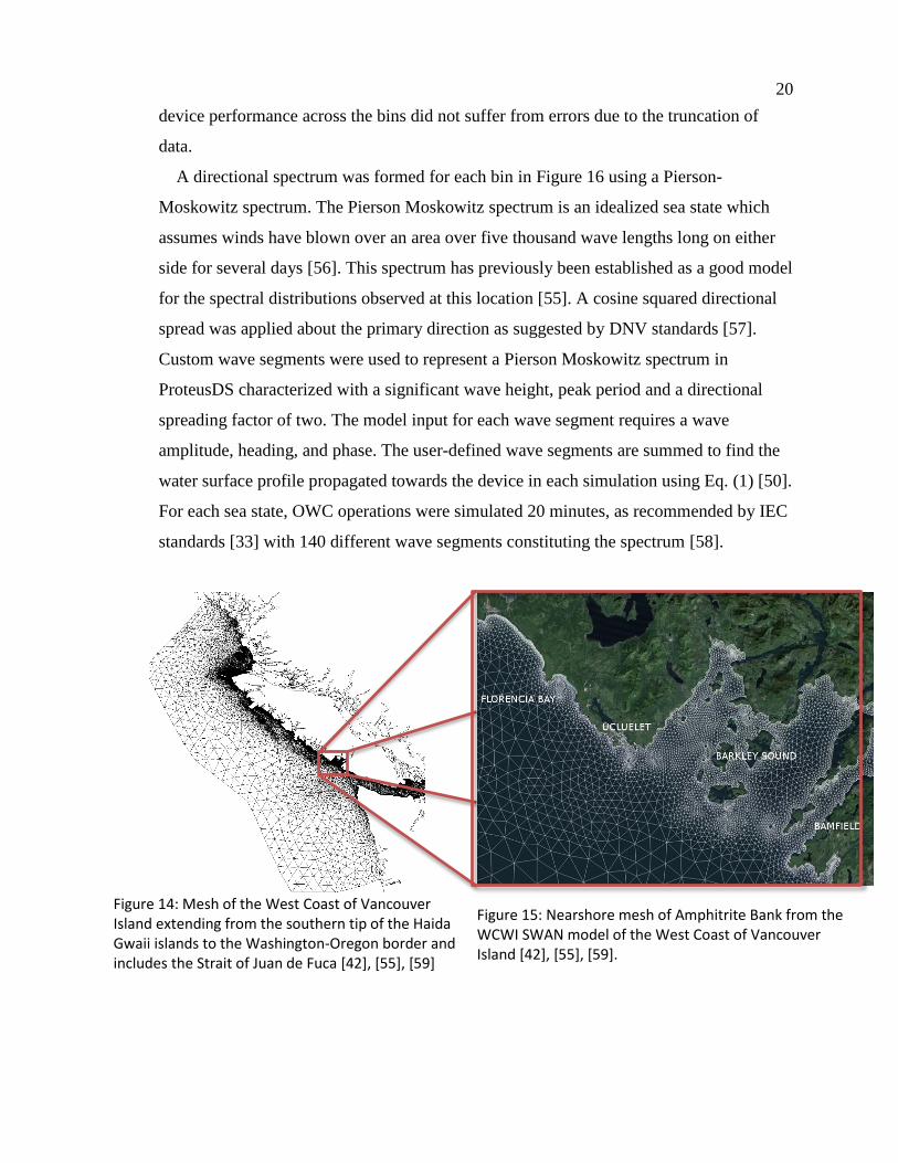
device performance across the bins did not suffer from errors due to the truncation of
data.
A directional spectrum was formed for each bin in Figure 16 using a Pierson-
Moskowitz spectrum. The Pierson Moskowitz spectrum is an idealized sea state which
assumes winds have blown over an area over five thousand wave lengths long on either
side for several days [56]. This spectrum has previously been established as a good model
for the spectral distributions observed at this location [55]. A cosine squared directional
spread was applied about the primary direction as suggested by DNV standards [57].
Custom wave segments were used to represent a Pierson Moskowitz spectrum in
ProteusDS characterized with a significant wave height, peak period and a directional
spreading factor of two. The model input for each wave segment requires a wave
amplitude, heading, and phase. The user-defined wave segments are summed to find the
water surface profile propagated towards the device in each simulation using Eq. (1) [50].
For each sea state, OWC operations were simulated 20 minutes, as recommended by IEC
standards [33] with 140 different wave segments constituting the spectrum [58].
Figure 14: Mesh of the West Coast of Vancouver Island extending from the southern tip of the Haida Gwaii islands to the Washington-Oregon border and includes the Strait of Juan de Fuca [42], [55], [59]
Figure 15: Nearshore mesh of Amphitrite Bank from the WCWI SWAN model of the West Coast of Vancouver Island [42], [55], [59].

21
Figure 16: Number of times each sea state occurred at Amphitrite Bank in 2006 at a
three hour resolution. Sea states that occurred for less than 24 hours have been truncated.
1.7 Preprocessing Simulations and Results
Each sea state identified in Figure 16 was simulated using the simulation architecture
previously described. Both of the ProteusDS and Simulink output data were consolidated
to produce a complete history of the motions of the OWC, hull, the three mooring lines
and the massless piston (representing the internal water column) as well as all the forces
and moments acting on these bodies. The kinematic data sets included output for each
relevant DOF of each body. Relevant DOFs are those in which significant energy transfer
occurs.
The author has extracted as much information as possible regarding the WEC’s
operation and response to incident wave conditions from the time domain simulators.
Detailed force and velocity time series were collected from the incident wave, the OWC
hull, the water column, PTO and moorings allowing the author to calculate the transfer of
energy between these components.
If one examines Figure 17 and takes the time series on the left (force in heave) and
conducts an element by element multiplication with the values on the right (velocity in
heave), the product of these values is a time series of power which integrated over time
results in an energy.

22
Figure 17: Time Series of the Incident Loading (right) on the OWC body in heave and the velocity of the body (left) in heave
The forces calculated within the time domain can be used to determine the device’s net
force contribution on the surrounding fluid domain. These contributions are then
translated into an energy can be incorporated into a spectral model, such as SWAN as
will be further discussed in Section 3.5.7.
1.8 Key Contributions
Although we have amassed high fidelity datasets with respect to the WEC, no
information pertaining to the device’s impact on the wave or how the surrounding fluid
domain is being impacted is explicitly provided. The work presented in this thesis
suggests taking the dynamics of a single WEC modelled in the time domain and back
calculating the device’s hydrodynamic losses and net force contribution onto the
surrounding sea. A meta-model capable of representing the interaction between the
device and the surrounding fluid domain is generated for the reference WEC allowing for
a better representation of devices deployed in an array. This static representation can
then be applied in between nodes within SWAN allowing for the device’s impact on the
surrounding wave field to be realized within the wave model.
By developing and testing candidate meta-models of the reference WEC, the current
work will contribute to the field of wave energy conversion in the following ways:
1. Developing a computational framework for transforming the simulated dynamics
of a single WEC (i.e. time histories of forces and velocities) into both temporally

23
and spectrally resolved descriptions of the power transfer (both directions)
between the incident waves and the WEC.
2. Establishing candidate tabular representations, or meta-models, of the spectral
power transfer that occurs over a variety of wave conditions that are compatible
with coastal wave models, such as that shown in Figure 14. Here, a
“representation” includes the tabulated results and a physically justified means of
inserting those tabulated results into the governing equations of the coastal model.
3. Establishing the sensitivity of the final system outputs (i.e. the far field impacts
and the WEC array power production) on the choice of candidate WEC
representation. Through these sensitivity studies, the work also contributes an
estimate of the uncertainty in the process.
4. Implementing the candidate meta-models within an existing large scale coastal
model based on the SWAN software and for a case of a very large commercial
scale farm (tens to hundreds of WECs), identifying any technical impediments and
testing means of negotiating these challenges.
1.9 Thesis Outline
The remainder of this thesis is laid out as follows:
Chapter 2 includes an overview of previous work that has been conducted in the field
of array modeling. The works are divided by the governing equations for each of the
models. In conclusion, a brief description of the model physics used to model arrays for
the remainder of this thesis is presented.
Chapter 3 outlines how a device is characterized within SNL-SWAN. Previous device
characterizations developed by SNL are described. This is followed by a detailed account
of where power is transferred when a device extracts power from an incident wave. This
power transfer demarcation is then used to generate a hydrodynamic meta-model for the
device. Chapter 3 is concluded with a description of the author’s newly proposed
methods to characterise a device within SNL-SWAN.
Chapter 4 presents the methodology used to compare the different methods used to
characterise a device, as presented in Chapter 3. The difference in annual power

24
production and far field impact of a device in each of these characterizations is analysed
in a numerical test basin as well as applied to a field case.
Chapter 5 reviews unresolved issues in the present work.
Chapter 6 summarizes the key conclusions of this thesis and presents
recommendations for future work in the development of a spectral wave array modelling
tool.

25
Chapter 2 Literature Review
The wave energy community has progressed in addressing the operational challenges
associated with single device deployment. The advances made to date are sufficient for
the pre-commercial stage of device development but the installation of a single device
will be insufficient to meet the power production needs of larger communities. To truly
make WECs commercially viable, tens to hundreds of WECs will need to be deployed in
an array. The installation of WECs in farms would result in cost savings associated with
moorings, electrical connections and maintenance [24]. However, as with any emerging
technology there are a number of unanswered questions regarding the operation of arrays
that need to be addressed.
Power production from an array may be smaller or larger than the sum of the power
produced by an equivalent number of independently sited WECs due to the power
absorbed and radiated by the hydrodynamic interaction of closely spaced devices [24],
[60]–[63]. Utilities are interested in determining how much these array interactions
impact the total power produced by the array and what configuration would ultimately
produce the most power. Wave energy developers are conversely interested in how a
control strategy can be adopted to produce the most power in an array. Additionally,
numerical and scale model tests of small WEC arrays have demonstrated wave height
attenuation between the WEC array installation site and a downwave location [26], [27],

26
[62], [64]. Wave field modifications caused by WEC array installations can influence
neighbouring coastal ecosystems, coastal defence structures and industries [62].
Regulators are concerned with the extent of wave height attenuation at the shoreline and
how this attenuation will impact pre-existing uses. As the field of WEC array design and
analysis advances, it is growing more evident that one universal computational
framework cannot effectively address all these concerns.
It appears that even within the narrow field of WEC array modeling, there exists a
creative choice a modeller must make to address the research question at hand. Previous
works have proposed frameworks that best address the primary concerns of electric
utilities and regulators - namely the energy yield and far-field impact of an array. Given
the large time scales and spatial domains utilities and regulators are interested in, a
computationally inexpensive model is crucial for these analyses.
Prior research largely draws from coastal wave models previously used to quantify the
wave attenuation associated with natural or manmade obstructions in the nearshore.
These models obtain realistic wave parameters in coastal areas and estuaries from given
wind, bottom and current conditions [65]. The definition of an obstruction, or obstacle
has changed as wave models have developed. Third generation wave models such as
SWAN were originally developed to model how waves change as they approach a
shoreline [66]. Obstructions, or obstacles, can be defined as a number of things. Natural
obstructions such as submerged reefs can reduce the wave energy transmitted to shore.
Man-made structures such as groins or breakwaters are built to prevent sediment
transport and consequently beach erosion as waves break along the shore [67].
Significant changes to the nearshore wave field are made by both natural reefs and
breakwaters as a result of wave overtopping, breaking over the crest, permeability
through the structures and wave diffraction [67]. The main physical processes involved in
wave transformation over and around submerged breakwaters are wave shoaling,
reflection, refraction, diffraction and breaking. Transmission coefficients used to
characterise these structures in nearshore wave models have typically been calculated for
such obstacles by using empirical formulae dependent on the incident wave height,
structure width, depth, etc. [68], [69].

27
A constant transmission coefficient may be appropriate for a static structure however,
the response of a moored, wave-generating device will change depending on the incident
wave condition. As a result, the transmission coefficient representation previously
adopted for static structures cannot sufficiently represent the dynamic responses
associated with WECs. The representation of an obstacle for breakwaters and WECs
alike varies from one coastal model to the next.
This chapter provides an overview of literature in which arrays of WEC devices have
been modeled in an effort to quantify the far field impact of a device. The benefits and
short comings of these models are presented followed by a discussion of the model
chosen for the remainder of this work.
2.1 Fundamentals of Wave Modelling: Airy Waves
Over the past 150 years deep water surface gravity waves have been conveniently
characterized with Airy wave theory based on both the conservation of mass and
momentum upon which kinematic and dynamic boundary conditions are imposed. The
conservation of mass is the foundation of the Laplace Equation [4]. The velocity potential
function is a scalar function describing the particle velocity of the water. Particles cannot
leave the surface of the fluid or penetrate the bottom as specified by the kinematic
boundary conditions. An analytical solution to the Laplace equation with the
aforementioned kinematic boundary conditions is a harmonic wave as described in Eq.
(1) [50]. The free surface displacement, 𝜂, is defined as:
𝜂 = 𝐴 𝑐𝑜𝑠(𝜔𝑡 − 𝑘(𝑥𝑐𝑐𝑜𝑠(𝜃ℎ) + ycsin(𝜃ℎ) + 𝜙) (1)
where 𝐴 is the wave amplitude, 𝜔 is the angular wave frequency, 𝑘 is the wave number,
𝜃ℎ is the wave heading (direction), 𝜙 is the wave offset (phase) and 𝑥𝑐, 𝑦𝑐 are the
coordinates with respect to a user-defined reference frame.
This convenient representation comes as a result of fundamental simplifications. It is
assumed the fluid medium is incompressible, inviscid, maintains a constant density and is
continuous15 [4]. Wave amplitudes are also assumed small compared to the wave length
and the water depth. These assumptions are violated in shallow water conditions where
15 Water can be discontinuous if there are air bubbles present, often occurring when waves break.

28
waves are steeper and viscous effects such as bottom friction impact a wave’s motions
[4].
Representing ocean waves as harmonic and independent waves has conveniently
allowed for the use of mathematical tools such as Fourier transformations and the
representation of polychromatic seas by wave spectra. A wave spectrum is a
representation of the sea surface at any instant in time by characterising the waves at a
particular location with respect to their amplitude, frequency and direction. The sea
surface at any point in time and at any location can be reproduced as a sum of a large
number of harmonic wave components which represent the surface displacement, as seen
in Eq. (2):
𝜂 =∑∑𝐴𝑖,𝑗𝑐𝑜𝑠(𝜔𝑖𝑡 − 𝑘(𝑥𝑐𝑜𝑠(𝜃𝑗,ℎ) + ysin(𝜃𝑗,ℎ) + 𝜙𝑖,𝑗)
𝑄𝑓
𝑖=1
𝑄𝑑
𝑗=1
(2)
where 𝜂 is the surface displacement, 𝐴 is the wave amplitude, 𝜔 is the angular wave
frequency, 𝑘 is the wave number, 𝜃ℎ is the wave heading, 𝜙 is the wave offset (phase)
and 𝑥, 𝑦 are the coordinates with respect to a user-defined reference frame, 𝑖 is the index
for the number of frequency bins, Qf, and 𝑗 is the index for the number of directional bins,
Qd. Even though there may be an infinite number of frequencies and directions that
characterize a sea state, these properties must be discretized into a certain number of bins
for feasible computation. By applying a Fourier analysis, the values of the amplitude and
phase can be determined for each frequency, as can be seen in Figure 18. For most deep
water wave records the phase information will have values varying between 0 and 2𝜋
without any preference for one value. The phase information is discarded and a uniform
distribution for phase is assumed. To reduce sampling bias, the Fourier analysis is
repeated over a number of observations and the mean amplitude spectrum is used to
characterize the sea condition [4].
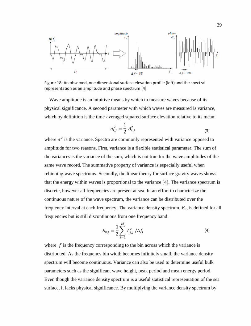
29
Figure 18: An observed, one dimensional surface elevation profile (left) and the spectral representation as an amplitude and phase spectrum [4]
Wave amplitude is an intuitive means by which to measure waves because of its
physical significance. A second parameter with which waves are measured is variance,
which by definition is the time-averaged squared surface elevation relative to its mean:
𝜎𝑖,𝑗2 =
1
2 𝐴𝑖,𝑗2
(3)
where 𝜎2 is the variance. Spectra are commonly represented with variance opposed to
amplitude for two reasons. First, variance is a flexible statistical parameter. The sum of
the variances is the variance of the sum, which is not true for the wave amplitudes of the
same wave record. The summative property of variance is especially useful when
rebinning wave spectrums. Secondly, the linear theory for surface gravity waves shows
that the energy within waves is proportional to the variance [4]. The variance spectrum is
discrete, however all frequencies are present at sea. In an effort to characterize the
continuous nature of the wave spectrum, the variance can be distributed over the
frequency interval at each frequency. The variance density spectrum, 𝐸𝑣, is defined for all
frequencies but is still discontinuous from one frequency band:
𝐸𝑣,𝑖 =1
2∑𝐴𝑖,𝑗
2
𝑀
𝑗=1
/Δ𝑓𝑖 (4)
where 𝑓 is the frequency corresponding to the bin across which the variance is
distributed. As the frequency bin width becomes infinitely small, the variance density
spectrum will become continuous. Variance can also be used to determine useful bulk
parameters such as the significant wave height, peak period and mean energy period.
Even though the variance density spectrum is a useful statistical representation of the sea
surface, it lacks physical significance. By multiplying the variance density spectrum by

30
the water density and the gravitational constant the energy density spectrum, 𝐸𝑖, is
obtained:
𝐸𝑖 = 𝜌𝑔 1
2∑𝐴𝑖,𝑗
2
𝑀
𝑗=1
/Δ𝑓𝑖 (5)
where 𝜌 is the water density, 𝑔 is a gravitational constant. The energy density spectrum
demonstrates how wave energy is distributed across different frequencies. Overall, the
sea surface representation used by coastal wave models varies depending on the specific
phenomena (wave shoaling, refraction, diffraction, etc.), spatial and temporal resolution
required for a particular analysis. Wave models are typically categorized as either phase-
resolving (where the water surface elevation, wave amplitude, direction and phase are
tracked for each node in the grid) and phase-averaged (where the wave spectrum is
recorded at each node). The following section will review both kinds of models in further
detail.
2.2 Boussinesq Models
The Boussinesq equations originally developed in 1872 are capable of accounting for the
vertical structure of both the horizontal and vertical flow velocities in a wave field. The
derivation begins with the depth-integrated continuity equation and the Bernoulli
equation for surface velocity which are closed with a relation between the depth-averaged
velocity and the surface velocity [70]. The equations went largely unused until the
advancement of computing in the mid 90’s and onwards [71]. Since the original
development of the Boussinesq equations, more robust forms have been developed to
account for varying bathymetry and to operate in deep water [72], whereas before
solutions were limited to intermediate to shallow water before the surf zone [67]. These
models calculate the instantaneous water surface elevation at each point in the domain,
Certain software suites such as MIKE 21 BW will also calculate the phase averaged
statistical parameters and wave disturbance parameters [73]. Boussinesq models are most
appropriate when modeling waves with strong nonlinearities, otherwise the mild-slope
equation, addressed in Section 2.3, is preferred [67]. A more detailed derivation of a
recent and commonly used form of the Boussinesq equations is provided by Madsen et al.
[70]. This series of equations is largely of interest to those modeling harbour resonance,

31
seiches (standing waves), wave-wave and wave-current interaction because the horizontal
plane of wave propagation can be well resolved without having to account for the vertical
coordinate from the Navier-Stokes flow equations [74]. Boussinesq models are phase-
resolved, as a result wave phenomena such as shoaling, refraction, diffraction and wave
breaking can be represented making the model suitable for analyzing the impacts a WEC
array would have on the nearshore wave climate. While these models do predict
nearshore hydrodynamic effects well at a small scale (domains of ten wavelengths [75]) ,
they are too computationally intensive for modeling larger areas or long periods of time
(typical time steps on the order of minutes) [43]. An array of five interacting devices was
modelled by Venugopal and Smith near the Orkney Islands using an enhanced
Boussinesq solver [17]. The devices were modeled as both reflecting and absorbing
sponge layers, but porosities and reflection coefficients were not related to specific
devices – hypothetical porosities of 0,0.6, 0.7, 0.8 and 0.9 were applied. In conclusion,
Boussinesq models are favourable for analyzing device interactions on a small scale since
they can represent phase dependent wave transformation processes, such as radiation and
diffraction. Boussinesq models however, become too computationally expensive in
domains larger than a few kilometres or temporal durations greater than tens of hours.
2.3 Mild slope Models
Mild slope equations are based on the Hamiltonian theory of surface water waves
where the vertical coordinate has been eliminated for faster computation time [76]. These
equations describe the transformation of linear irregular waves across a slowly changing
bathymetry and have been used to compute wave transformations near offshore structures
for at least 40 years [77], [78] . Mild slope models calculate the instantaneous surface
elevations throughout the domain, with a relatively low computational and accuracy cost
and high stability [62].Two separate techniques have been used to represent WECs in
mild slope models.
Beels studied the wake effects of a single device and an array of overtopping WECs
using a mild slope model in both uni- and multidirectional waves [30], [77] where a
device is represented as a sponge layer covering the spatial extents of the WEC.
Absorption functions define the absorption of the device at each cell of the WEC in both
the x and y direction. Coefficient values were determined through tests in a numerical

32
wave tank where previously derived equations determining the overtopping discharge
were used to determine the device’s efficiency in different irregular seas [77].
Most recently, Babarit et al. [79] modelled a WEC within ARTEMIS, a mild-slope
model [79]. Babarit characterized the far field effect of a device with a Kochin function -
an asymptotic expression for an outgoing wave which superposes circular diffracted and
radiated waves generated by a device. This formulation was originally derived by Kochin
in 1940 but has found use in more recent naval architecture applications [45], [80]. The
Kochin function is found using the diffracted and radiated velocity potential associated
with the WEC calculated from a BEM solver. Given a particular incident wave condition,
a device will generate its own radiated and diffracted wave. The Kochin function sums
the complex amplitudes of the waves generated by the device at a user-defined far-field
point (or circle) [45]. The total far field potential is then converted to variance and input
back into the wave model. Mild-slope models have a low computational cost relative to
Boussinesq models with relatively high accuracy [43], but they still suffer from
numerical instabilities that arise due to rapidly varying topography and when waves shoal
in shallow waters [67], [81]. Mild slope models are also limited to smaller domains.
Generally, at least ten gridpoints per wave length are recommended and time steps should
be chosen based on a Courant number criterion, limiting the application of the model to
simulations on a minute to hourly scale [82].
2.4 Spectral Action Density Models
Rather than accounting for each wave individually, spectral action density models
follow the evolution of an entire wave spectrum across the model domain. At each
spatial node, the variance (or action density in the case of currents) is computed opposed
to the instantaneous water surface elevation which is calculated in both the Boussinesq
and mild slope models. Tracking the water surface elevation and phase is important for
characterizing wave phenomena such as diffraction and radiation however, the spectral
action density approach allows for a quick and numerically stable solution to wave
propagation by tracking variance and assuming a uniform probability distribution for
phase.
The model is capable of representing most wave nonlinearities such as wave breaking
and wave-wave interactions, as seen in Eq. (6). However, it cannot explicitly model

33
diffraction and thus employs a phase-decoupled numerical approximation for this
phenomenon [83], which is described further in Section 2.5. The governing equations
present how a wave spectrum evolves over the computational domain. The first three
terms on the left hand side of Eq. (6) denote the propagation of the wave energy spectrum
over time, t, and space x,y respectively. The fourth term represents the depth and current
induced refraction. Finally the fifth term on the left represents the effect of shifting
frequencies due to variations in depth and mean currents. The right hand side of Eq. (6)
contains source and sink terms that non-linearly redistribute energy. Action density is
conserved in the presence of currents, opposed to energy density and as such, the
evolution of action density over the computational domain is defined as:
𝜕𝑁(𝜎, 𝜃)
𝜕𝑡+ 𝑐𝑥
𝜕𝑁(𝜎, 𝜃)
𝜕𝑥+ 𝑐𝑦
𝜕𝑁(𝜎, 𝜃)
𝜕𝑦+ 𝑐𝜃
𝜕𝑁(𝜎, 𝜃)
𝜕𝜃+ 𝑐𝜎
𝜕𝑁(𝜎, 𝜃)
𝜕𝜎=𝑆
𝜎
(6)
𝑆 = 𝑆𝑤 + 𝑆𝑛𝑙3 + 𝑆𝑛𝑙4 + 𝑆𝑏𝑓 + 𝑆𝑤𝑐 + 𝑆𝑑𝑝
where N is the action density spectrum, 𝑐𝑥 and 𝑐𝑦 are the propagation velocities in spatial
x-y space, 𝑐𝜃 and 𝑐𝜎 are the propagation velocities in directional (𝜃) and frequency (𝜎)
space respectively [84]. The source terms (S) that are accounted for in most third
generation spectral action density models include wave growth by wind (Sw), triad wave
interactions (𝑆𝑛𝑙3), quadruplet wave interactions (𝑆𝑛𝑙4), wave decay due to bottom
friction (𝑆𝑏𝑓) and whitecapping (𝑆𝑤𝑐) and finally wave decay due to depth induced wave
breaking (𝑆𝑑𝑝).
Spectral action density models have been used to calculate wave transformations over
large areas in order to find accurate wave conditions near shorelines [85]. In recent years,
the use of these models has been extended to the study of a WEC array’s far field impact
particularly in the MIKE spectral wave model, TOMAWAC and Simulating WAves
Nearshore (SWAN) where WECs have been represented as bathymetric features, source
and sink terms at a node or as linear energy transmitting obstructions.
Greenwood et al. simulated WECs within the Danish Hydraulic Institute’s (DHI)
MIKE 21 spectral model using three techniques to simulate a WEC: a source term, an
artificial island and a reactive polygon. The reactive polygon was found to be the most
realistic method because it accounted for device specific frequency and directional
impact on the waves. |Downstream wave power was decreased by 5% on average and

34
upstream values increased by 7.5% on average indicating the importance of including
reflection within the representation of a WEC [86].
Folley and Silverthorne represented WECs as source and sink terms within
TOMAWAC, a spectral action density model developed at the Electricité de France's
Studies and Research Division. Frequency-dependent reflection and absorption are
characterized by these simulations based on a device’s hydrodynamic coefficients [31].
Silverthorne and Folley used a frequency dependent function to represent a WEC within
the model. The device’s inertial, radiation and damping forces were determined for the
case of maximum energy extraction and used as inputs into the model [31]. The authors
were able to capture radiation effects within the WEC array, enhancing a spectral wave
model’s capacity to calculate an array’s power performance.
The most advanced wave array depictions to date have been implemented in the software
SpecWEC, a module of the spectral domain model TOMAWAC developed by the
PeraWAT project between 2009 and 2013. This spectral domain model captures the non-
linear effects of a wave energy converter and uses phase-averaged approximations to
represent radiation. The SpecWEC software has been cross-validated with both the
numerical time-domain model WaveDyn as well as tank tests conducted at the Queens
University Belfast’s Portaferry wave tank [87],[63]. Child and Weywada compared the
performance of a 24 unit array of point absorbers in the SpecWEC model to experimental
results in a variety of spectral sea states. The difference in yield between the spectral-
domain and experimental results is between 3.6 and 14.4% with an average of 7.9%
which the authors considered a good level given the uncertainties in the experimental
tests. This study has confirmed that phase-averaged models can be reliable tools for
modelling WEC arrays [63].
SWAN has been used to model WEC arrays as both a single obstacle and a number of
obstacles [43], using a transmission coefficient specifying the percentage of energy
absorbed by the device [15], [88]. Millar et al. investigated the effects of WEC arrays in
SWAN by modelling entire arrays as four kilometre long partially transmitting obstacles
at the Wave Hub test site. These arrays were given transmission coefficients of 0, 70, 90
and 100%. The aforementioned transmission coefficients vary between complete
absorption of wave energy to zero absorption. Even in the worst case, where all wave

35
energy before the obstacle was absorbed, the maximum reduction in significant wave
height at the shoreline was 21.7%. Device specific parameters were not used in the study
and individual devices were not modelled [15]. Iglesias and Veigas confirmed Millar et
al.’s sensitivity analysis by conducting a similar analysis at a wave farm in Tenerife,
Canary Islands, Spain. Transmission coefficients of 0, 25, 75 and 90% were modeled to
see whether there were drastic changes in significant wave height (Hs), energy dissipation
due to bottom friction and directional spreading. The most drastic change in Hs was
observed between transmission coefficients of 75 and 90% with respect to changes in Hs
and energy dissipation. Directional spreading was increased in the central wake of the
farm and decreased around the edges [29]. Further nearshore wave climate studies were
conducted by Smith et al. in 2012. The authors modified the SWAN source code in order
to allow for user input of frequency and direction dependent coefficients within the
obstacle command. The authors of this study generated hypothetical power transfer
functions as input for transmission coefficients [88]. Porter modelled the far field impact
of a WEC array using nested grids within SWAN’s computational domain. Longshore
transects were chosen in between the rows of devices within an array. A spectral file was
output and modified outside of SWAN using a device specific transfer function. The
modified wave spectrum was used as the input for the next row of wave energy
converters within the array [89], which became the proof of concept for SNL-SWAN.
Recently, SNL-SWAN has improved the characterization of a device within a wave
model by modifying the standard obstacle command in SWAN to allow for both sea
state-dependent and frequency-dependent absorption characteristics emulating the
behavior of a device deployed in the ocean [28],[32]. The software contains an obstacle
switch command declared near the beginning of an input file identifying which device
parameterization will be employed for the simulation. The user can choose to implement
a constant transmission coefficient which reduces the wave spectrum by a uniform
percentage based on the wave spectrum’s significant wave height and peak period, or
have each frequency bin individually modified within the spectrum. The results of the
SNL SWAN software are validated with experimental array tests of 1:33 scale models of
the Columbia Power Technologies’ Manta 3.1 device [28]. Future releases of the

36
software will capture the effects of reflection and radiation [90]. A more in-depth review
of SNL-SWAN’s features is discussed in Section 3.2.
2.5 Model Selection
The spectral action density model was chosen as the most appropriate to model a WEC
array’s far field impact largely because it can propagate waves over a large domain with
low computational expense. The aforementioned Boussinesq and Mild slope models
solve for the instantaneous water surface elevation and resolve the complete horizontal
and vertical flow velocity structures for each constituent wave. While the Boussinesq and
mild slope models are suitable candidates for resolving radiation and diffraction around
wave energy converters, their computational expense limits their use to domains a few
kilometres wide, smaller WEC arrays and shorter time durations [31].
Resource assessments executed on large domains using these phase resolved models
will be compromised by slow execution speeds. In addition to the high associated
computational expense, these models suffer from numerical instabilities due to the stiff
nature of their governing equations. The computational domains studied in Boussinesq
and mild slope models are much smaller than those conducted in spectral action density
models. For instance, the wave resource assessment conducted for the West Coast of
Vancouver Island, Canada extends from the bottom of the Olympic Peninsula to just
below Haida Gwaii. The area covers over 410,000 square kilometres with over 130,000
computational nodes [55]. The model is capable of simulating a full year of boundary
conditions at a three hour resolution in less than two days on an eight core processor.
In addition to the spectral action density model’s computational efficiency, it is a tool that
is familiar to the wave energy industry. Present day wave energy resource assessments
are typically produced using spectral action density models [49], [55], [91]–[94].
As such, developing new methods for including WEC arrays within these models
presents a natural progression in accepted practices for wave energy resource assessment
[95]. Spectral action density models are capable of accounting for non-linear wave
phenomena such as bottom friction, wave breaking, quadruplet and triad wave
interactions. The use of source and sink terms to represent the aforementioned wave
phenomenon can similarly be extended to the representation of a WEC within a spectral
model.

37
The fundamental equations of all third generation spectral wave models (WAM,
WaveWatch III, SWAN, etc.) are in essence the same. The most prominent difference
between SWAN and the other spectral models is the numerical scheme used to solve the
spectral action balance equation. SWAN’s implicit formulation allows for larger time
steps and higher spatial resolution across both structured and unstructured grids. SWAN
is typically used for nearshore regions while the other models have been applied by
meteorological agencies on a global scale [96]. In addition to the suitability of SWAN’s
model physics and computationally efficient numerical scheme, the software is open
source which has resulted in its extensive academic and industrial use [87].
One of the largest criticisms faced by the selection of the SWAN model is that it is
phase-averaged and hence cannot accurately represent a WEC’s operation. Phase-
averaged models by definition do not store information regarding whether two waves are
in or out of phase with one another making phase-dependent processes such as radiation
and diffraction difficult to represent explicitly within spectral-domain solvers such as
SWAN [95]. Computing diffraction from fundamental phase dependent relationships
requires considerable computing effort. However, a phase-decoupled approach [97] is
employed in the SWAN model, which has been shown capable of portraying the spatial
redistribution of waves caused by the phenomenon. The approximation is based on the
mild-slope equation for refraction and diffraction omitting phase information [98].
Given advances made in modelling diffraction, it is conceivable that future work may
identify candidate techniques for mimicking the effects of radiation in spectral action
density models like SWAN with similar success if information of a WEC’s motion could
also be incorporated in the model’s governing equations. Even without these future
developments in hand, studies have suggested that phase information is irrelevant when
realistic wave conditions and array configurations are considered [99].
Folley and Whittaker conducted a statistical analysis of WEC array interaction factors
to determine how accurately phase information could realistically be calculated. Incident
waves, the WEC array layout and the devices’ dynamics were considered in this analysis.
The authors determined incident waves are typically represented with two-parameter
spectra which poorly represent bimodal sea states underlining the uncertainty in the
model’s boundary conditions [49], [99], [100]. In cases where wave spectra are generated

38
using a wave model, it should be noted that models are typically calibrated using Hs
where uncertainties are typically 5% and wave periods have a root-mean squared error of
approximately two seconds [99]. In real deployments, there will be uncertainty in the
WEC’s exact positions due to device drift and moorings. Furthermore, environmental
conditions such as tides and currents can affect the transit time for a wave traveling
towards a device changing the wave’s phase relationship [99]. Lastly, variation in
individual device motion can be restrained by differences in manufacturing tolerances
and marine growth.
Given the uncertainty associated with a device’s operation in real seas, it appears
randomized phase is an adequate assumption when modelling WEC arrays under realistic
conditions. In conclusion, the SWAN model is computationally efficient, capable of
covering large domains and employing long time steps, familiar to the industry and has
been proven to be adequate for modeling WECs given its phase-averaged nature. As
such, the WEC characterization proposed in this thesis is implemented within SWAN.

39
Chapter 3
Wave Energy Converter
Characterization
The obstacle command in SWAN was originally designed to represent breakwaters as
straight line barriers that could be placed between gridlines within the modeled domain.
An obstacle modifies the propagation of energy across a line proportionally to a user
defined parameter. In the present SWAN formulation, this parameter is a simple
percentage of energy transmitted, which can be arrived at either experimentally or with
empirical formulations [68], [69].
In the case of WECs, numerically generated time series data (such as that generated in
Section 1.7) provide a good understanding of how energy is removed from the incident
wave field [18]–[22]. However the challenge arises in being able to chart this
understanding in a simplified representation (something at the fidelity of a SWAN
model’s representation of the wave conditions) that can be used to adjust the obstacle’s
parameters on-the-fly to model the frequency and direction dependencies of the WEC’s
performance.
This chapter presents a detailed review of how a WEC is presently represented in SNL
SWAN. The remainder of this Chapter develops a method with which to increase the

40
fidelity of the device’s energy conversion process, ultimately capturing the interaction
between the incident wave and the primary interface. In Section 3.4 an energy balance
analysis is presented that examines how time domain data defining the forces acting
between the WEC, the incident waves and the radiated waves can be processed to
determine the total energy transfer to the WEC, the energy lost to dissipative effects (eg.
drag) and the energy returned to the surroundings as radiated waves. An overview of the
different forces acting between the wave, and the subsequent exchanges of mechanical
work between the two entities, and the WEC are presented in Section 3.5. In Sections 3.6
and 3.7, the outputs of the energy balance analysis are transformed into two new
proposed obstacle cases – obstacle case five and obstacle case six which are each a form
of meta-model of the wave-WEC interaction.
3.1 Existing Methods for WEC performance characterization
Within SNL SWAN, a wave energy converter’s representation has been crafted based
on WEC performance data generated by a WEC developer. This data is generally in the
form of power matrices or relative capture width curves (RCWs). A power matrix is a
table of average mechanical power produced by a WEC over a range of sea states. Sea
states are typically characterized by parameters derived from spectral moments (defined
below). Power matrices for WECs have been characterized by the significant wave height
and peak period of the incident sea in order to work within the framework previously
outlined by Sandia National Labs, although energy period has been recommended by IEC
standards [33]. The significant wave height was traditionally defined as the mean wave
height of the highest third of waves, however, as sea states are being resolved by their
wave spectra, it is defined as four times the standard deviation of the water surface
elevation [4]:
𝐻𝑠 = 4√𝑚0 (7)
where the spectral moment of 𝑛𝑡ℎ order, 𝑚𝑛, uses Eq. (8) when calculating from the
non-directional variance density spectrum using:
𝑚𝑛 =∑𝑓𝑖𝑛𝑆𝑖Δ𝑓
𝑖
(8)
where Δ𝑓 is the frequency increment and 𝑓𝑖𝑛 is the 𝑖𝑡ℎ frequency to the 𝑛𝑡ℎ power.

41
The peak period, Tp is the wave period with the highest energy and is defined as:
𝑇𝑝 =1
𝑓𝑝
(9)
where 𝑓𝑝 is the frequency bin with the greatest variance density in the spectrum.
RCW curves present a WEC’s relative power absorption at different frequencies [65].
Each entry in a RCW curve is a ratio of the power absorbed to the incident power
available in the sea [65]. Each entry in a performance matrix is for a group of irregular
waves while the RCW curve tracks performance across a series of independent, regular
waves.
An example of the performance matrix and the RCW curve are presented in Figure 19
and Figure 20 respectively. The data provided in Figures 19 and 20 is only a portion of
the energy extraction completed by the WEC; these figures show the power produced by
the PTO – not the power that was extracted from the wave itself. As they do not show
the full value of power extracted from the incident wave, these tabulations cannot wholly
account for a device’s hydrodynamics in a coastal model.
Figure 19: Typical power matrix in which the power captured by the device is reported in a bin corresponding to a sea state characterized by an Hs and Tp
Figure 20: Typical RCW where the percentage of power captured by the device is reported as a function of incident wave frequency [65]
RCW curves are typically generated by performing regular wave tank tests for waves of
different frequencies. From these tests, a monochromatic or polychromatic capture width
curve can be derived [11]. Price has demonstrated the capture width in irregular seas is
lower than in a monochromatic sea of corresponding period [11]. As such, directly
employing an experimental monochromatic RCW curve would overestimate the device’s
power capture in an irregular sea.

42
Within the wave energy community at large there is a tendency to use the term ‘power
absorbed’. This term can be used to describe a number of power phenomena – be it the
power that is transferred to the device’s exterior hull (manifesting in kinetic energy), or
the power captured by the device’s PTO (manifesting in a useful energy commodity like
electricity or pressurized fluid). This overarching use of power absorbed has resulted in
confusion as to which power capture stage is being referenced. In an effort to settle any
confusion surrounding the discussion of power capture, Price outlines four stages over
which a device captures power [11], as pictorially represented in Figure 21.
Figure 21: Power transfer stages of a WEC [11]
The ‘intercepted power’ is defined as the power flow between the incident wave and
the device’s primary interface [11]. Kinetic and potential energy in the incident wave
perform work on the hull of the WEC creating kinetic energy in the WEC structure. The
WEC’s kinetic energy does work on the surrounding fluid and radiates new waves while
non-linear hydrodynamic forces (drag) dissipate kinetic energy from both the incident
wave and the WEC.
Some kinetic energy in the WEC is subsequently stored in the short term as potential
energy and some is fed into the PTO. The energy flow through the PTO is defined as the
‘captured power’. Captured power is the rate of production of a useful energy
commodity.
Finally, there is the power flow between the PTO output and the final product used by
the consumer, the ‘delivered power’, which is generally electricity but other commodities
could be pressurized air, desalinated water, pressurized hydraulic fluid, etc. A WEC’s
delivered power is the final output of a series of energy conversion processes.
When attempting to model the interaction of a WEC with the incident wave, it is obvious
that the hydrodynamic losses and the power transferred back into the water via radiated

43
waves must be accounted for if a WEC array is to be modeled accurately. Unfortunately,
these energy fluxes are either not tabulated by WEC developers, or not made publically
available.
This chapter seeks to address two central challenges outlined in the preceding
paragraphs. For one, a new device representation is proposed to capture the varying
degrees of complexity in a WEC’s operation. While a linear, offshore structure can be
effectively represented in the spectral domain with a single percentage of energy
transmitted or reflected, a dynamic device is more difficult to accurately represent since
the levels of intercepted, captured and delivered power vary greatly with the incident
wave conditions (eg. frequency, direction, wave height, etc.). Secondly, the metrics with
which the device’s power capture is reported is placed under critical review. The author
proposes the use of the intercepted power as a means with which to characterize the
device’s impact on the surrounding waves. Using intercepted power to represent the
WEC device includes hydrodynamic losses and the power radiated by the device back
into the fluid domain.
3.2 Existing SNL SWAN Obstacle cases
In SWAN, the location of an obstacle is defined by a sequence of node points used to
represent line segments. Obstacles interrupt the propagation of the waves from one grid
point to the next [101]. This interruption can be in the form of wave reflection, wave
absorption or even a wave source, such as the injection of energy at a new frequency
when a device radiates waves.
In SWAN’s representation of static obstacles, the transfer of energy through an obstacle
is defined by the user with a transmission and or reflection coefficient. A transmission
coefficient extracts a ratio of incident wave energy in space, as seen in Eq. (10). This
coefficient is traditionally the ratio of Hs incident to the obstacle and Hs in the lee of the
obstacle [102]. However, given energy is proportional to Hs2, the transmission
coefficient, Kt is also squared in Eq. (10). The transmission coefficient is applied at
linkages between nodes across which action density propagates, as such it is applied to
the spatial derivatives of the action density formulation previously employed in Eq. (6):
𝜕𝑁(𝜎, 𝜃)
𝜕𝑡+ 𝑐𝑥
𝐾𝑡2𝜕𝑁(𝜎, 𝜃)
𝜕𝑥+ 𝑐𝑦
𝐾𝑡2𝜕𝑁(𝜎, 𝜃)
𝜕𝑦+ 𝑐𝜃
𝜕𝑁(𝜎, 𝜃)
𝜕𝜃+ 𝑐𝜎
𝜕𝑁(𝜎, 𝜃)
𝜕𝜎=𝑆
𝜎
(10)

44
where 𝐾𝑡 is the transmission coefficient.
SNL-SWAN currently characterizes a WEC using either the aforementioned power
matrix or RCW curve. Each obstacle case uses one of these data sets to generate a
transmission coefficient allowing for the extraction of energy from the incident sea [103].
When a captured power matrix is employed, the wave energy transport at the node
incident to the obstacle line is first calculated. The Hs and Tp are calculated from the
incident spectrum. Bilinear interpolation is used to find the respective power captured for
the corresponding sea state [65]. The energy flux incident to the obstacle is the sum of the
potential and kinetic energy being transported by a wave in the direction of wave
propagation:
J = ∫ ∫ 𝑐𝑔𝐸(𝜎, 𝜃)𝑑𝜎𝑑𝜃 (11)
𝐸(𝜎, 𝜃) =𝜌𝑔
2𝜂2(𝜎, 𝜃)
(12)
where J is the omnidirectional wave power transport also referred to as energy flux. The
energy density can be derived from the spectral action density equation. Action density is
typically used in SWAN’s formulations as it is conserved in the presence of currents
while energy density is not [84]. Action density and energy density are related by
frequency:
𝑁(𝜎, 𝜃) =𝐸(𝜎, 𝜃)
𝜎
(13)
The transmission coefficient (K2t ) [32] is used to characterize the device’s power
capture for a particular wave condition. The transmission coefficient is simply a ratio:
𝐾𝑡2 =
𝑃𝐿𝑒𝑒𝑃𝐼𝑛𝑐
= 1 −𝑃𝑐𝑎𝑝
𝐽 ⋅ 𝑤
(14)
where 𝑃𝐼𝑛𝑐 is the energy flux incident to the device, and 𝑃𝐿𝑒𝑒 is the remaining energy
flux in the lee of the device, 𝑃𝑐𝑎𝑝 is the power captures by a device’s power take-off and
w is the width of the device. Within the calculations of a SWAN model, the transmission
coefficient is calculated by interpolating the captured power from a power matrix. The
captured power is normalized against the total incident wave energy flux. The total
incident wave energy flux is scaled by the characteristic width of the device. The width
parameter is subject to debate as a device can intercept more power than is present in the

45
length of wave crest corresponding its own width. The remainder of the energy flux is
assumed to pass through the device thus defining the percentage of power transmitted.
When an RCW curve is employed to characterize device performance, the transmission
coefficient is found by subtracting one from the relative capture width indexed for the Tp
incident to the WEC. By employing a RCW curve, the device developer has already
decided what w should be as RCWs are reported as a percentage of the incident energy
captured from the surrounding sea as a function of frequency.
The way the transmission coefficient is used in SNL-SWAN depends on the obstacle
case selected. Within SNL-SWAN, the user has the option to use one of five WEC
representations, referred to as obstacle cases.
Obstacle case zero corresponds to the standard SWAN obstacle command which
extracts a certain percentage of the incident wave energy applied across all sea states and
frequencies.
Obstacle case one uses a power matrix to calculate a transmission coefficient
dependent on the significant wave height and peak period of the incident sea state. The
same coefficient is applied uniformly across all frequencies in the energy density
spectrum [65].
Obstacle case two employs an RCW curve to calculate a constant transmission
coefficient across all frequencies [65]. The peak frequency (Tp-1) incident to the device is
found within the RCW curve input by the user. Obstacle case two was not investigated in
this analysis. Although regular wave simulations could have been run in the time domain
simulator, the computational expense of these tests was deemed too high given these tests
would not be representative of a device’s behaviour at sea.
Obstacle case three employs a revised power matrix to determine the transmission
coefficient for each frequency bin in the incident energy spectrum. The input to this
module differs from that of obstacle case one. The axes along the edges of the power
matrix are Hs and period (T), opposed to the Hs and Tp used in obstacle case one. SNL-
SWAN determines the Hs incident to the device. The row in the power matrix is then
used as an RCW curve. A separate transmission coefficient is determined for each entry
in the RCW curve and then applied to the respective frequency in the incident variance

46
density spectrum [90]. Obstacle case three requires the construction of a modified power
matrix generated from experimental tests that are not commonly used in practice [104].
Obstacle case four employs an RCW curve to determine a transmission coefficient for
each individual frequency bin. These values are independent of the incident sea state
[65]. As previously outlined, applying a monochromatic RCW curve will overpredict the
device’s optimal performance at certain frequencies [11]. A more detailed description of
each of the existing obstacles are present in the SNL-SWAN User Manual available on
the SNL-SWAN website [32].
In general, the author has concluded power matrices better characterize a device’s
performance because they are indexed against more spectral characteristics of the
incident, polychromatic sea state, and thus a power matrix should give a more accurate
measure of captured power. The new WEC representations presented later on in this
chapter will only be compared to obstacle case one.
3.3 Limitations in Existing SWAN WEC Representations
There are three chief weaknesses in the representation of WECs in SNL SWAN, the
first stems from the device’s geometric representation while the second and third result
from the data used to characterize the device. The device is represented with a line of a
specified device width orthogonal to a grid node. Given directionality is not considered in
this analysis, having the user input angled devices into the model domain could lead to
erroneous results. During SNL-SWAN execution, a directional spectrum is stored at the
incident node. For each bin of the incident spectrum, the directional energy transport can
be calculated and projected into x and y Cartesian components, as presented by the dark
blue vectors in Figure 22. A transmission coefficient is applied between two adjacent
nodes, representing the WEC partially absorbing the energy moving between those two
nodes. The WEC only affects the energy incident to the device and as such, the
transmission coefficient is applied only to the x-projection of the wave energy vectors
presented in Figure 22. The representation of a WEC as a line becomes problematic for
certain geometries or device configurations. For attenuator devices such as Pelamis for
instance, the device is narrow but very long, when represented as a line, the device will
inevitably absorb more power than is available at the incident node since the total
incident energy flux is set by the node spacing of the SWAN grid. That node spacing is

47
set based on preconceived notions of what the WEC device’s actual width w is. As
mentioned earlier, for some choices of w the RCW can be greater than one. This
shortcoming will be further discussed in Section 5.1.1 and will not be addressed in this
thesis.
Figure 22: Representation of an obstacle within SWAN. The device is represented as a line across which energy can be transferred. A transmission coefficient is applied to the x projection of the incident energy (energy propagated perpendicular to the obstacle) while energy in the y-projection is not impacted by the device’s operation.
The second limitation in the device’s representation is that directional information
concerning the incoming waves is ignored. The omnidirectional power transport is used
to determine a transmission coefficient which is then applied to each of the directional
bins in the energy spectrum. A further discussion on how the incident power transport in
obstacle case five and six is presented in Sections 3.6 and 3.7 respectively.
The third limitation in the device’s representation is the user provided information used
to characterize the device. The reliance of Obstacle cases 0 through 4 on developer
supplied captured power matrices and RCW curves raise questions concerning the
accuracy of the existing SNL SWAN WEC representations. Developers must supply
performance information to clients and regulators to develop projects and thus this level
of data is easy to attain. The derivation of a transmission coefficient from this data alone
assumes that any effect the WEC has on the surrounding sea state is represented solely by

48
the captured power. In short, by using these pre-existing parameterizations perfect
conversion from incident to mechanical power is assumed, and the energy removed from
the incident waves is likely to be underestimated.
3.4 Device Power Balance
The contributions of power leaving and entering the WEC device are presented in
Figure 23. The power contributions on the left hand side correspond to the power
entering the device from the fluid domain. The power contributions on the right
correspond to power leaving the device. There are two pathways that can be taken when
power leaves the device. Firstly, power can permanently leave the system, as is done
when mechanical power is extracted through the PTO. Second, power can be transferred
back to the device. For instance, a device can work off of its own radiated wave, or in the
case of drag, the direction of power transfer depends on the device’s relative velocity to
the surrounding fluid.
Within the control volume of the reference WEC there are also internal oscillation of
potential and kinetic energy between the device’s two bodies. Even though this internal
energy transfer can be extracted from the time series data, there is no need to do so as no
additional information concerning the device’s impact on the surrounding fluid is gained.
Figure 23: Visual representation of a device’s power transfer. Kinetic and potential energy is transferred between the reference WEC’s two bodies. The yellow arrows indicate the direction of power transfer into and out of the reference WEC.
3.5 Force and Power Contributions during Device Operation

49
The following section describes the nature of the models employed by the time domain
simulator to calculate the forces acting on the reference WEC. This is necessary in order
to give the reader a sense of the inevitable modelling errors and how they may influence
the final power balance. First, the Equations of Motion for a surface piercing rigid body
is described in Section 3.5.1. This explanation is followed by a description of the
individual force calculations and their extension to power transfer.
3.5.1 Equations of Motion
The dynamics of a semi-submerged WEC can be described by the Equations of Motion
for a floating, surface piercing, rigid body. Equation (15) describes the equations of
motion for each of the reference WEC’s two bodies:
𝑴�̈�(𝑡) + 𝑨(∞)�̈�(𝑡) − ∫ 𝒌(𝑡 − 𝜏)�̇�(𝜏)𝑑𝜏𝒕
𝟎
− 𝑪𝒙(𝑡) − 𝑭𝑷𝑻𝑶(𝑡)
−𝑭𝒎(𝑡) − 𝑭𝒗(𝑡) − 𝑭𝒊𝒓(𝑡) = 𝑭𝑬(𝑡)
(15)
where 𝑴 is the mass of the object, 𝑨(∞) is the object’s added mass at infinite frequency.
Both these variables are 6 x 6 matrices indicating the body’s mass and added mass in
each DOF. The degrees of freedom include three translational modes and three rotational
modes which are described in further detail in Table 3. The variable 𝒌(𝑡 − 𝜏) is an
object’s impulse response kernel, 𝑪 is the object’s 6 x6 hydrodynamic stiffness matrix,
and finally 𝒙 is a 6 x 1 vector indicating the device’s position in six DOF. 𝑭𝑷𝑻𝑶
represents the damping forces and moments induced by the power take-off (PTO). 𝑭𝒎
represents the damping forces exerted by the moorings in the translational degrees of
freedom. 𝑭𝒗 represents the damping forces and moments induced by viscous drag. 𝑭𝒊𝒓
represents the internal reaction forces induced by the second body on the first which can
at times lead to energy permanently being dissipated due to internal drag. Finally, 𝑭𝑬
corresponds to the excitation force and moments induced by the incoming wave. Each of
the terms 𝑭 are 6 x 1 vectors with the first three entries corresponding to forces acting on
the device in surge, sway and heave, and the last three entries corresponding to moments
acting on the device in roll, pitch and yaw. Certain rotational degrees of freedom may
have negligible moment contributions due to the irrotational fluid assumption, which will
be further addressed in the remainder of Section 3.5. The power transfer due to these

50
loads is calculated by an inner product on the instantaneous force and velocity. The
power transfer and equations of motion for the hull are demonstrated in the heave degree
of freedom in the following section and can be applied by analogy to the light piston
representing the internal water. The equations can be applied to each relevant degree of
freedom, as specified in the following sections.
3.5.2 Power Transfer due to Wave Excitation
The excitation force is the sum of the pressure exerted across the body due to the
presence of the incident and diffracted wave which can also be defined as the sum of the
Froude-Krylov and scattering forces. The Froude-Krylov force, defined as the force due
to the pressure field of an undisturbed wave[45], while the scattering force is the pressure
field due to the wave diffracting around the body. Due to linear superposition, these
combine to form the excitation force:
𝐹𝐸 = ∫𝑝(𝑠)𝒔
𝑛𝑑𝑆 (16)
where 𝑝(𝑠) is the pressure across the surface of the object16, 𝑛 is the normal vector to the
surface, and s is the surface of the body. The excitation force is only applied in the
translational degrees of freedom as flow is assumed to be irrotational. ProteusDS
calculates the incident loading at any given moment in time, based on the wave
amplitude, relative heading, phase offset and wave frequency of the incident wave for
each degree of freedom [50]. The incident loading generated from each regular wave
component of the irregular sea state and the total incident wave spectrum is summed
together to generate a time series of the excitation force. This excitation force, FE, is then
multiplied by the velocity of the body:
𝑃𝑖𝑛𝑐,𝑏 = 𝐹𝐸 ⋅ �̇�𝐵 (17)
to determine the power from excitation imparted on each body (the hull or the piston).
3.5.3 Power Transfer due to Radiation
The radiation force results from the body oscillating in the absence of an incident wave
[45]. The radiation force at any given moment in time is calculated from the convolution
16 The pressure is the sum of the pressure from the incident wave and the scattered wave.

51
of body motions at previous time steps with impulse response kernels and the added mass
at infinite frequency multiplied by the acceleration of the body [54]. The total radiation
force is the sum of two calculations done in parallel. The radiation force exerted by the
body and the piston onto the external waves is calculated within ProteusDS. The second
radiation force is calculated within Simulink and corresponds to the internal radiation
force between the piston and the body and the radiation force exerted by the body onto
the piston. The radiation components are delineated in the heave equation of motion:
𝑀�̈�(𝑡) + 𝐴(∞)�̈�(𝑡)⏟ 𝑅1
−∫ 𝑘(𝑡 − 𝜏)�̇�(𝜏)𝑑𝜏⏟ 𝑅2
𝑡
0
− 𝐶𝑥(𝑡) − 𝐹𝑃𝑇𝑂(𝑡)
−𝐹𝑚(𝑡) − 𝐹𝑣(𝑡) − 𝐹𝑝,𝑣(𝑡) = 𝐹𝐸(𝑡)
(18)
where R1 is the radiation component corresponding to the added mass at infinity and R2 is
the force calculated with the impulse response kernel from the added damping values.
Radiation is present in all six degrees of freedom. The added damping and added mass at
infinity parameters are calculated in WAMIT, as outlined in Section 1.5.1. WAMIT
returns 6 x 6 matrices for 𝑨(∞) and the kernel functions to calculate the force and
moment acting on the body due to radiation at any point in time. The motion of the water
column within the OWC’s air chamber results in a force radiated onto the hull as well as
a force exerted onto the water column as it induces motion in the otherwise still water.
Separate added mass and damping coefficients determined through generalized modes, as
described in Section 1.5.3, were entered into Simulink in order to determine the radiation
contributions between the hull and the water column. The total radiation forces acting on
the OWC are a sum of the radiation produced by the hull, and the radiation produced by
the piston. The power associated with radiation is found by multiplying the radiation
forces by each body’s respective velocity to determine the radiated power exerted on
each body:
𝑃𝑅𝐴𝐷,𝑏 = (𝑅1 + 𝑅2) ⋅ �̇�𝐵 (19)
The radiated power is negative when it is acting on the fluid surrounding the device.
3.5.4 Power dissipated through Moorings
Mooring forces are calculated in ProteusDS using a cubic-spline lumped mass cable
model [51]. The model accounts for each cable segment’s material properties such as the
bending, flexural, torsional and axial rigidity [20]. The finite element discretization

52
evaluates viscous drag forces, and internal bending, torsional and axial forces at each
node point within a cable for its mass and frequency independent added mass. A more
detailed account of the cable dynamics can be found in the ProteusDS manual [50], [51].
This mooring force is multiplied by the cable’s velocity where it is attached to the body
for each linear DOF. The power dissipated from the moorings is found with:
𝑃𝑚𝑜𝑜𝑟 = 𝐹𝑚𝑜𝑜𝑟 ⋅ �̇�𝐶 (20)
Where 𝑃𝑚𝑜𝑜𝑟 is the power dissipated through the moorings and �̇� describing the velocity
of the cable at its insertion points at the device. The force and power associated with the
moorings is only found in the translational degrees of freedom in ProteusDS.
3.5.5 Power Transfer due to the PTO
The OWC is modeled as a dynamic system that is coupled to the thermodynamics of
an air chamber. The hull of the device is modeled as a six DOF body and the water
column within the chamber is simulated as a piston resting on the water column [20]. The
hull and piston were modeled in the time domain. The mean mechanical power produced
by the OWC in each sea state was determined from the product of the force between the
two bodies and their relative velocity. The force on the water column was calculated from
the area of the air chamber and the pressure differential between the air chamber and
atmosphere, with the force on the hull being equal and opposite to this.
3.5.6 Power Transfer due to Viscous Drag
The drag forces experienced by the OWC are calculated for each panel of the body’s
mesh that is below the undisturbed water surface elevation. The force of drag is
calculated using the relative velocity between the fluid and the device. Empirical
coefficients are used within ProteusDS in order to calculate the drag force. Given the
OWC’s typically low Keulegen-Carpenter number, a drag coefficient of three is used
based on experimental results for a rectangular cylinder in oscillatory flows [20], [105].
The drag force acting on the device is defined by:
𝐹𝑣 =1
2𝜌𝐶𝑑𝐴𝑝𝑟𝑜𝑗(�̇�𝐵 − �̇�𝑊)|�̇�𝐵 − �̇�𝑊|
(21)
where Aproj is the projected area of the mesh panel, 𝐶𝑑 is the drag coefficient, 𝑥�̇� is the
velocity of the device and 𝑥�̇� is the velocity of the water. The drag force is found in all

53
translational and rotational degrees of freedom however the angular velocity of the water
was assumed to be zero as a result of the irrotational flow assumption.
The direction in which the drag force is acting depends on the relative velocity between
the device and the surrounding fluid. Drag is inherently different from the other forces
previously discussed in this section because it transfers power not only between the wave
and the body, but also dissipates power to the surrounding fluid in the form of a wake.
Power transfer is dependent on the magnitude of the power associated with each agent
as well as the direction in which each agent is moving, as is illustrated in Figure 24.
In order to isolate the energy that is being transferred to the device from the fluid and
vice versa, the time series of the power induced by drag was separated into contributions
inducing motion and contributions resisting motion as a result of three power transfer
scenarios which are dependent on the relative velocity between the device and the water.
Power is always transferred from the medium with greater energy to that of lower energy.
An equivalent magnitude force is applied upon either agent (body or water), with only a
change in direction implying the direction of power transfer (body to water, or water to
body) which can be determined based on the relative velocity of these bodies.
The general power transfer equation is presented in Eq. (22). When the velocity of the
water is greater than that of the body the fluid is transferring power to the body, thus
inducing motion (im). In the second scenario presented in Eq. (22), the velocity of the
water is less than that of the fluid, meaning the device is resisting the motion of the fluid
and power is being transferred back into the wave. In each case, some of the power
transferred between the fast body and the slower body is being permanently dissipated to
the ambient fluid. In the third scenario, if at any point in time the velocity of the body and
fluid are the same, no power is transferred between the two mediums.
𝑃𝑑𝑟𝑎𝑔,𝑦 = 𝐹𝑣 ⋅ �̇�𝐵 {𝑦 = 𝑖𝑚 (�̇�𝑤 − �̇�𝐵) > 0
𝑦 = 𝑟𝑚 (�̇�𝑤 − �̇�𝐵) < 0
(22)
In addition to the drag associated with the body, there is an additional drag force
associated with the fluid. The fluid drag is defined as:
𝑃𝑑𝑟𝑎𝑔,𝑓 = 𝐹𝑣 ⋅ �̇�𝑊 (23)

54
where power is being transferred back into the fluid as a wake. The direction of power
contributions from the body and the water based on the direction and magnitude of each
body’s velocities are illustrated in Figure 24.
It should be noted that work that is done on the incident wave, is lost within the present
formulation in the time domain simulator. ProteusDS does not increase the energy in the
incident wave based on the drag force, which may be a source of error in the power
balance presented in Section 3.5.7.
Figure 24: Scenarios in which power can be transferred from one medium to another as a result of drag. vB is the velocity of the body, vW is the velocity of the water.
3.5.6.1 Power from Internal Reaction Forces
The internal drag of a fluid within the OWC’s body is comprised of viscous losses,
turbulent losses and vortex transport [20]. A representative drag coefficient of 0.02 was
used to represent the drag experienced by oscillating flows in a cavity without significant
wake [20], [106]. The cavity drag was calculated within Simulink and is defined as:
𝐹𝑝,𝑣 = −1
2𝜌 𝐴𝐵,𝑖𝑛𝑡𝐶𝑝,𝑑 (�̇�𝑝 − �̇�𝐵)|�̇�𝑝 − �̇�𝐵|
(24)

55
where 𝐴𝐵,𝑖𝑛𝑡 is the area of the wetted interior in the OWC, 𝐶𝑝,𝑑 is the internal drag
coefficient, �̇�𝑝 is the velocity of the piston and �̇�𝐵 is the velocity of the body. The power
that is dissipated by internal reaction forces (drag transferring power between the two
bodies) is then dissipated to the ambient fluid as a wake is calculated using:
𝑃𝑖𝑛𝑡,𝑝 = 𝐹𝑝,𝑣 ⋅ (�̇�𝑝 − �̇�𝐵) (25)
The heave force and power presented here can be further extended to the internal
reactional forces in all translational degrees of freedom.
3.5.7 Device Meta-model
The hydrodynamic impact of the device on the surrounding fluid can be characterized
by the power absorbed by the device which is defined as the difference between the
power incident to the device, and the power radiated from the device:
𝑃𝐴𝑏𝑠 = 𝑃�̿� − 𝑃𝑅̿̿ ̿ (26)
where the total power incident to the device is defined in Eq. (27) and the total radiated
power is defined by Eq. (28). The total wave power incident to the device is a sum of the
incident wave contributions and the power contributions of drag inducing motion:
𝑃𝐼̿̿ ̿ = 𝑃𝑖𝑛𝑐,𝑝 + 𝑃𝑖𝑛𝑐,ℎ + 𝑃𝑑𝑟𝑎𝑔,𝑖𝑚 (27)
where 𝑃𝑖𝑛𝑐,𝑝 is the product of the incident loading force on the piston and the velocity,
𝑃𝑖𝑛𝑐,ℎ is the product of the incident loading on the OWC hull and the velocity of the hull,
𝑃𝑣,𝑝𝑜𝑠 is the product of the positive contribution of the viscous drag on the body and the
body’s velocity. The total power radiated by the device into the surrounding fluid domain
is the sum of the radiation and cross radiation power contributions defined by
𝑃𝑅̿̿̿̿ = 𝑃𝑟𝑎𝑑,𝑝 + 𝑃𝑟𝑎𝑑,ℎ + 𝑃𝑟𝑎𝑑,𝑝2ℎ + 𝑃𝑟𝑎𝑑,ℎ2𝑝 (28)
where 𝑃𝑟𝑎𝑑,𝑝 is the product of the radiated force of the piston and the velocity of the
piston, 𝑃𝑟𝑎𝑑,ℎ is the product of the radiated force of the body and the velocity of the body,
𝑃𝑟𝑎𝑑,𝑝2ℎ is the product of the radiated force the piston exerts on the body within the OWC
air chamber and the velocity of the piston, 𝑃𝑟𝑎𝑑,ℎ2𝑝 is the product of the radiated force the
OWC body exerts on the piston and the velocity. The cross radiation terms are only
present in the translational degrees of freedom.

56
The total incident and the total radiation power terms are input into SNL-SWAN as
separate input files. The power absorbed is determined internal to SNL-SWAN based on
the parameters set by the user. As previously presented in Figure 23, the power absorbed
(which includes power dissipated and mechanical power produced) includes:
𝑃𝐴𝐵𝑆 = 𝑃𝑃𝑇𝑂 + 𝑃𝑑𝑟𝑎𝑔,𝑓 + 𝑃𝑑𝑟𝑎𝑔,𝑟𝑚 + 𝑃𝑚𝑜𝑜𝑟 + 𝑃𝑖𝑛𝑡,𝑝 (29)
The total power absorbed by the device and its constituents are the foundation upon
which obstacle cases five and six were built. Theoretically, either side of the power
balance can be used represent a device’s hydrodynamics.
3.5.8 Validation of the Power Flow Calculation
The power balance presented in Eq. (26) was carried out for each sea state in which the
reference device was modelled. In general, there was good agreement between the two
methods with an average root mean squared error of 4.0% between the left and right hand
sides of Eq. (26). Most of this error is present in sea states with low Hs values (less than
two metres). A portion of the errors reported in Figure 25 can be attributed to the inexact
calculation of the fluid drag force. The velocity of the water could only be obtained at the
device’s center of gravity which in reality varies along the different panels of the device’s
mesh.
Figure 25: Root mean squared error between the right and left hand sides of the power balance formulation

57
3.6 Obstacle Case Five
Applying a transmission coefficient calculated from the ratio of the incident wave
power and captured power implies perfect conversion from incident to mechanical power.
In real seas, this assumption can lead to erroneous representations of the far field impact
of a WEC array. Obstacle case five seeks to remedy this oversight by using the device
meta-model generated in Section 3.5.7 to represent a device in a way that is simple
enough to keep SWAN computationally efficient but also capture’s the device’s
hydrodynamic impact on the surrounding fluid domain.
Obstacle case five is very similar in structure to that of the previous obstacle cases
created by SNL. The device is represented as a line, as depicted in Figure 22 and applies
a constant transmission coefficient across each frequency and directional bin of the
variance density spectrum propagating incident to that line. The difference in the newly
proposed obstacle case lies in which parameters are used to calculate the obstacle
transmission coefficient. The transmission coefficient is determined by the ratio between
the total power absorbed by the device and the power in the waves. The power absorbed
can be defined as either the right hand side or left hand side of Eq. (26), depending on the
information the user has available. The power in the waves is calculated by taking the
projection of the incident wave energy flux in the direction perpendicular to that of the
obstacle in SWAN.
Theoretically, the user could characterize radiation as a process that occurs both
incident to and in the lee of the device. Representing a device as both a source and a sink
more realistically describes the device’s behaviour by expressing the device’s absorption
and radiation of power. This method is invoked when the user specifies the inclusion of
radiation in the model’s start-up switches. An addition radiation case (radcase) switch
has been added to the SNL-SWAN control file for this purpose.
When the radiation case switch is enabled, the transmission coefficient is alternatively
defined as:
𝐾𝑡,𝐹 = 𝜅𝑡,𝑖𝑛𝑐 − (1 − 𝛾𝑟𝑎𝑑) ⋅ 𝜅𝑡,𝑟𝑎𝑑 (30)
where 𝜅𝑡,𝑖𝑛𝑐 is calculated from the ratio of the incident power to the device and the power
in the waves, 𝜅𝑡,𝑟𝑎𝑑 is calculated from the ratio of the radiated power, specified in the

58
radiated power matrix and the power in the waves and finally 𝛾𝑟𝑎𝑑 is the user-specified
percentage of power radiated back towards the incident wave.
Additionally, 𝐾𝑟 is calculated which is defined as the percentage of power in the waves
that is reflected from the device. The reflection coefficient is used to represent power that
is being put back into the fluid domain by the device through radiation and is defined as:
𝐾𝑟 = 𝛾𝑟𝑎𝑑 ⋅ 𝜅𝑡,𝑟𝑎𝑑 (31)
This approach is consistent with the way energy transmission is represented in SWAN,
however not necessarily consistent with the way radiated power is transferred physically.
As a result, the shape of the radiated wave field will be a scaled representation of the
incident wave field.
There are logistical constraints associated with employing obstacle case five where too
much power can be removed from the system if not enough radiation is put into the lee of
the device and the transmission coefficient exceeds one. A transmission coefficient
greater than one implies that the device is taking more power out of the sea than is
physically available. As such, in order to properly employ the radiation case programmed
in by the author, the condition presented in Eq. (32) must be true.
𝐾𝑟 + 𝐾𝑡 < 1 (32)
The power absorbed by the device is determined by calculating the difference between
the energy available at the incident node and the energy radiated or transmitted to the
next node. If 𝛾𝑟𝑎𝑑is set to one, the device acts as a sink, and will only be able to take
energy from the waves propagating towards the device. In this characterization, two
transmission coefficients are calculated. The traditional power matrix used in obstacle
case one, is used to determine the captured power produced by a device. This
transmission coefficient 𝐾𝑡,𝑃𝑇𝑂 is used by SNL-SWAN to determine the captured power
produced by each device in the simulation and is output to the user in a text file. A
second transmission coefficient 𝐾𝑡,𝐹 is calculated using the novel power absorbed matrix.
The ratio between the power absorbed and power in the waves is used to generate a
transmission coefficient which is applied to the wave spectrum as it crosses an obstacle
and is used to determine the far field impact of the device.

59
3.7 Obstacle Case Six
While obstacle case five is able to represent the device’s hydrodynamic impact on the
surrounding wave climate, it still cannot resolve how a device responds to waves of
different frequencies. Since most devices are tuned to a particular frequency bandwidth,
frequency dependence is crucial when characterizing the performance of a device. RCW
curves were previously used by SNL to characterize devices in obstacle cases two and
four which parameterize a device’s performance in regular waves according to its
frequency. Even though a device is represented as a linear system, it is difficult to justify
using an RCW curve to characterize a device’s performance in irregular waves. In regular
waves, resonance at certain oscillation frequencies can overestimate a device’s
performance.
As a device encounters different sea states, it is expected that its performance at each
frequency will also change. In order to account for this variability in operation, an RCW
matrix is proposed as an input into obstacle case six which captures the frequency
dependent performance of a device in each incident sea state. Given the performance of a
device is based on the Hs, Tp and now frequency/period, an additional dimension is added
to the power matrix. The relative capture width matrix can be most simply described as a
three dimensional array as presented in Figure 26.
Figure 26: Visual representation of the relative capture width matrix structure

60
The variables M, and N correspond to the number of Hs and Tp bins used to
characterize the sea states that occur over the course of a representative year. The RCW
matrix stores transmission coefficients for a user-defined number of periods along the
axis extending into the page. The periods specified by the user can vary between sea
states and do not have to be evenly distributed. A transmission coefficient is linearly
interpolated from the curve for each frequency bin within the SWAN simulation. Section
3.7 describes how the RCW matrix is generated.
Obstacle case six is very similar to obstacle case five. Both modules characterise a
device based on the total power intercepted by the device, rather than the captured power.
The two modules differ primarily in that obstacle case six assigns a different transmission
coefficient, 𝐾𝑡,𝐹 to each frequency, and that the RCW matrix is a pre-calculated ratio
when it is input into SNL-SWAN, opposed to absolute power stored in the power
absorbed matrix.
In obstacle case six, a transmission coefficient 𝐾𝑡,𝑃𝑇𝑂 is calculated using a power
matrix, as outlined in Section 3.6. The second transmission coefficient 𝐾𝑡,𝐹 is found by
bilinearly interpolating the first two dimensions of the RCW Matrix. A row
corresponding to the device’s frequency dependent operation has been identified. A
transmission coefficient 𝐾𝑡,𝐹 is interpolated for each frequency bin used in the SNL-
SWAN model
3.7.1 Relative Capture Width Matrix Generation
The following section provides a detailed description of how one can generate an
RCW Matrix from the time series data provided by the device architecture models
outlined in Section 1.3. Traditionally, an RCW curve presents the ratio of captured power
produced by a device to the power available in the waves at that frequency. In an
irregular sea, there is a different amount of power available at each of the frequency bins.
WEC developers tune their devices to operate optimally within a certain frequency range.
As a result, a device will not extract the same percentage of power from each frequency
bin. An RCW curve is generated for each sea state to determine what percentage of the
power in the waves is absorbed (or radiated). The structure and procedure to generate an
RCW curve is universal but the contents of the RCW Matrix depend on the input data (ie.

61
incident power, radiated power or power absorbed). For the purposes of demonstration,
the remainder of this section describes the generation of an RCW curve for the power
incident to a device.
First, Section 3.7.1.1 describes how the incident power in the waves at each frequency
is determined, which is the denominator for the RCW presented in Eq. (14). Second,
Section 3.7.1.2 describes how the power incident to the device is transformed from the
time domain into the frequency domain, providing the numerator term in Eq. (14).
Finally, Section 3.7.1.3 will conclude the section by demonstrating how the two
frequency representations of power are used to determine the RCW curve for a sea state.
3.7.1.1 Wave Power in the Frequency Domain
Each time domain simulation is forced with individual sinusoidal waves with varying
amplitudes, frequencies and directions to represent an incident wave spectrum which are
converted into energy fluxes used as the denominator term in Eq. (14).
The wave amplitude associated with each frequency bin in the wave spectrum is
converted to a variance. Variance associated with waves of different directions but falling
within the same frequency bin were summed ultimately leaving the wave spectrum
dependant only on frequency. The group velocity associated with the mean frequency of
each frequency bin changes according to the depth across which a wave propagates and
the dispersion relation [107]. Group velocity in intermediate water depth is defined as:
𝑐𝑔 =𝐿
2𝑇[1 +
4𝜋𝑑
𝐿 sinh (4𝜋𝑑𝐿 )
]
(33)
where 𝐿 is the wave length, 𝑇 is the wave period, 𝑑 is the depth of water. The wave
energy transport associated with each frequency bin is calculated using the discretized
form of Eq. (11). The reader should note that all directional components of the incident
wave spectrum are used to calculate the power incident to the device, while in obstacle
case five only the orthogonal components of the energy flux were used to calculate the
power in the waves.
3.7.1.2 Representation of Device Power in the Frequency Domain
A generic approach to determining the frequency dependent device power in a given
sea state is presented. The device power can be either: the power absorbed by the device,

62
or a combination of the power incident to and radiated from the device depending on the
input file the user wishes to generate. The following section will use the power transfer
due to the wave excitation force as a case study to demonstrate how a force and velocity
time series can be reconstructed into a frequency domain representation of power.
Power is a product of an instantaneous force and velocity which are both readily available
from the time domain simulation results generated in Section 1.5. The incident force
exerted across each panel in a device’s mesh is recorded for each time step and DOF over
the course of the simulation. Velocity is similarly recorded for each body in the device
and each DOF. The first 200 seconds of each times series is removed to eliminate start-up
transients. The left hand side of Figure 17 presents the incident loading time series for the
OWC body in heave. The right hand side of Figure 17 presents the velocity time series
for the OWC body in heave.
Second, a Fast Fourier Transform (FFT) is conducted for the force and velocity time
series data. The number of samples in the FFT is equivalent to the number of time steps
in the signal. A high sample number was employed in order to resolve high frequency
oscillations, ensuring the original signal variance is conserved. The FFT decomposes the
time series signal into regular sinusoids. The FFT assigns an amplitude and phase to each
frequency present in the time series signal. The amplitude spectrum corresponding to a
device’s incident loading in heave is presented on the left hand side of Figure 27 while
the spectrum associated with the device’s velocity in heave is presented on the right.
Figure 27: Force and Velocity Amplitude Spectrums for a single DOF in a sea state of Hs = 1.75 m and Tp=11.1 s.

63
The inset in the left and right hand side of Figure 27 show the sinusoidal wave
associated with each of the frequency bins in the amplitude spectrum which have been
recreated for each frequency bin in the spectrum. The water surface elevation is
calculated using the non-directional form of Eq. (1):
𝜂𝑖 = 𝐴𝑖 cos(𝜔𝑖𝑡 + 𝜙𝑖) (34)
A power signal is generated by taking the product of the time series force and velocity
signals presented both in Figure 28 and in each of Figure 27’s insets. The mean value of
this power signal corresponds to the power absorbed by the device at that frequency, as
depicted in Figure 29.
Figure 28: Force and velocity time series signal associated with a frequency of 0.1 Hz for a body in heave
Figure 29: Power time series signal generated as a product of the force and velocity time series signals in Figure 28
It should be noted that after performing an FFT, the number of frequency bins
produced by the transformation is equivalent to the number of samples in the input time
series. As a result, the number of frequencies associated with the device’s incident power
spectrum is greater than that of the wave power (since SWAN works with a user
specified number of frequencies, which in this study is 40). In order to generate an RCW
curve, the incident power spectrum must be rebinned to correspond to the same frequency
bins propagated through the ProteusDS simulation domain.
In order to rebin the signal, each of the incident spectrum frequency bins is assigned
and grouped into a wave power frequency bin. Each grouped bin is worked with
individually. The sinusoidal power signals associated with each of the frequencies within

64
the grouped bin are summed to generate a cumulative power signal. The grouping of bins
and summation of signals for the power signal data is pictorially represented in Figure 30.
Figure 30: Summation of power signals to rebin into the same frequency bins as used in the incident wave spectrum.
The mean of this cumulative power signal is assigned to the grouped frequency bin.
The methodology outlined above was conducted for a single incident loading force on the
OWC’s hull in heave. Section 3.7.1.3 describes how the rebinned frequency domain
power signal is used to generate an RCW curve.
3.7.1.3 RCW Matrix Generation
An RCW curve is the ratio of the frequency resolved device power, for which the
procedure was described in Section 3.7.1.2 and the frequency resolved wave power found
in Section 3.7.1.1. In order to account for all the power incident to the device, the
procedure outlined in Section 3.7.1.2 must be repeated for each force incident on the
device in each DOF. The total power incident to the device is a summation of power
contributions previously noted in Equation 15. Each of these power contributions is
related to a force and velocity time series found in the time domain simulations. The time
series data is processed using the methodology presented in Section 3.7.1.2 and summed.
Once the total power incident to the device is found, a ratio of the wave power spectrum
and the incident power spectrum is taken. The two power spectrums are presented on the
left hand side of Figure 31 with the resulting RCW curve on the right.

65
Figure 31: Power in a Hs = 1.75m and Tp = 11.1s sea state and power absorbed by the device overlayed on the left. RCW curve associated with this sea state on the right.
The RCW curve associated with a particular sea state is placed in the third dimension
of the RCW matrix where the first two dimensions are chosen based on the index of the
Hs and Tp characterizing the sea state.
Theoretically, either side of the power balance in Eq. (26) can be used to generate an
RCW curve, as was previously described in Section 3.5.7. For the purposes of this work,
the RCW curve for each sea state was generated from an average of the two curves.
The approach presented in Section 3.7 allows the user to spectrally resolve the power
transfer between the device and the surrounding fluid for each particular power
contribution. However, by applying an FFT, we assume that the force assigned to a
particular frequency bin has been generated as a result of the wave power in the same bin.
Generating an RCW curve involves summing the spectrally resolved power of the
contributions outlined in Figure 23. The power contained in each frequency bin can be
either positive or negative depending on whether the power in this bin is leaving or
entering the device. Even though this method can establish a general representation of the
device’s dynamics, the transfer of power from one frequency bin to the next due to
nonlinear forcings cannot be resolved. As such, there are instances in which the power in
certain frequency bins exceeds the energy flux associated with the incident wave
spectrum, described in further detail in Section 5.1. It is beyond the scope of this thesis to
determine the origins of this excess energy, but in an effort to make the proposed method
tractable, power in excess of the incident wave spectrum was redistributed to
neighbouring bins. This procedure was applied for two reasons. First, at these

66
frequencies, it is implied that the device is extracting more power than is physically
available in the incident wave spectrum, violating the conservation of energy within
SWAN. Second, in order to make obstacle case five and six consistent, the power
absorbed by the device in each obstacle case would need to be the same (ie. the sum of
each spectral power component must be the same as the total power absorbed by the
device in a particular sea state in obstacle case five).
A post-processing step was employed where the RCW curve for each sea state was
analyzed. If at a particular frequency the power exceeded that of the incident wave
spectrum, the excess power at that frequency would be distributed to the frequency bins
to the left and right. In cases where the neighbouring bins are already saturated, power
would be shifted to the next neighbouring bin. The nearest bins would always be
saturated first, followed by the successive neighbouring bins. Three illustrative cases for
rebinning excess power in a particular frequency bin are presented in Figure 32 to Figure
34. First, if there is excess power absorbed by the device, depicted by the red cross-
hatched area in Bin 13, and there is wave energy available in the two neighbouring bins
(12 and 14), the excess power absorbed will be evenly distributed across the two bins.
Figure 32: Redistribution of energy flux when there is enough available wave energy transport available in both neighbouring bins. The blue bins are the wave energy transport in the incident sea. The yellow bins correspond to the relative capture width at that period.
In the second case presented in Figure 33, if there is power absorbed by the device in
excess of the available wave energy (Bin 16), and one of the neighbouring bins is already
saturated (Bin 17), the excess power is transferred into Bin 15. The final case in which
energy is rebinned is presented in Figure 34. The excess power absorbed by the device in

67
Bin 15 is first shifted into its two immediately neighbouring bins (Bin 14 and 16). After
the neighbouring bins are saturated, the rebinning algorithm moves into the next
neighbouring bin, Bin 13.
Figure 33: Redistribution of energy flux when there is only enough available wave energy transport in one of the two neighbouring bins. The blue bins are the wave energy transport in the incident sea. The yellow bins correspond to the relative capture width at that period.
Figure 34: Redistribution of power when the two neighbouring bins are saturated. The blue bins are the wave energy transport in the incident sea. The yellow bins correspond to the relative capture width at the same period.

68
3.8 Novel Obstacle Case Summary
The representation of a dynamic, wave-generating device within a wave modelling
software can take many forms. SNL has proposed using the obstacle command within
SWAN to represent a WEC. The work presented in this thesis seeks to add a degree of
higher fidelity to this representation and ultimately determine what the limitations to this
representation are. The obstacle command in SWAN was originally designed to represent
breakwaters as straight line barriers that could be positioned along gridlines within the
modeled domain. SNL refers to this command as obstacle case zero. A constant
percentage of the incident wave energy is extracted across all sea states and frequency
bins.
The WEC representations developed by SNL seek to characterize a device based on
information available to utilities and regulators from device developers. In practise,
device developers are most concerned with power capture performance and thus report
captured power metrics. The derivation of a transmission coefficient from these metrics
alone assumes any effect the WEC has on the surrounding sea state is represented solely
by the power captured by the device – energy losses and radiated energy are unaccounted
for. To better represent the device’s impact on the surrounding fluid domain, the author
has developed WEC representations that account for both the device’s captured power as
well as the device’s intercepted power.
Obstacle case five bilinearly interpolates a transmission coefficient from an intercepted
power matrix, uniformly reducing the variance in each frequency bin of the incident
spectrum. The intercepted power is used to calculate the device’s impact on the
surrounding fluid domain while the captured power is used to determine the power
produced by the device.
Obstacle case six applies a sea state and frequency dependent transmission coefficient
to the incident variance spectrum. This transmission coefficient is calculated from the
RCW Matrix. As in obstacle case five, the intercepted power is used to calculate the
device’s impact on the surrounding fluid domain while the captured power is used to
determine the power produced by the device. Obstacle case six is a higher fidelity
representation of a wave energy converter however without further validation it is

69
difficult to determine which of the two novel obstacle cases is more accurate. Each WEC
representation presented in this Chapter is summarized in Table 4.
The conservation of intercepted power between obstacle cases five and six is analyzed.
The power contributions of the PINC, PRAD, and PABS terms presented in Eqs.(15) through
(29) are conserved to a great degree between obstacle cases five and six. On average, the
mean root square error of the incident power and the radiated power, presented in Figure
35 and Figure 36 is 0.34% and 1.14% respectively. The radiated power is prone to more
error as the force and velocity contributions come from two separate models (a
hydrodynamic ProteusDS model and a thermodynamic Simulink model) which were
modeled at different time resolutions. In addition, there were more radiation force
contributions resulting in a greater summative error.
Figure 35: Percentage difference between the bulk incident power and the sum of the spectrally resolved incident power in each sea state
Figure 36: Percentage difference between the bulk radiated power and the sum of the spectrally resolved radiated power in each sea state
The root mean squared error, averaged for each modelled sea state, between the bulk
power employed in obstacle case five and the summation of the spectrally resolved power
terms from obstacle six is 0.13% and 2.04% for PABS and PINC-PRAD respectively. The
error between the two is presented for each sea state in Figure 37 and Figure 38. In
general, the spectrally resolved representation of power sums to a lower value as a result
of minor losses in power due to FFT windowing and potential leakages within bins. The
difference in the LHS of the power balance (PINC-PRAD), is generally greater than that of
the right because it is composed of more power contributions. Again, the greatest error
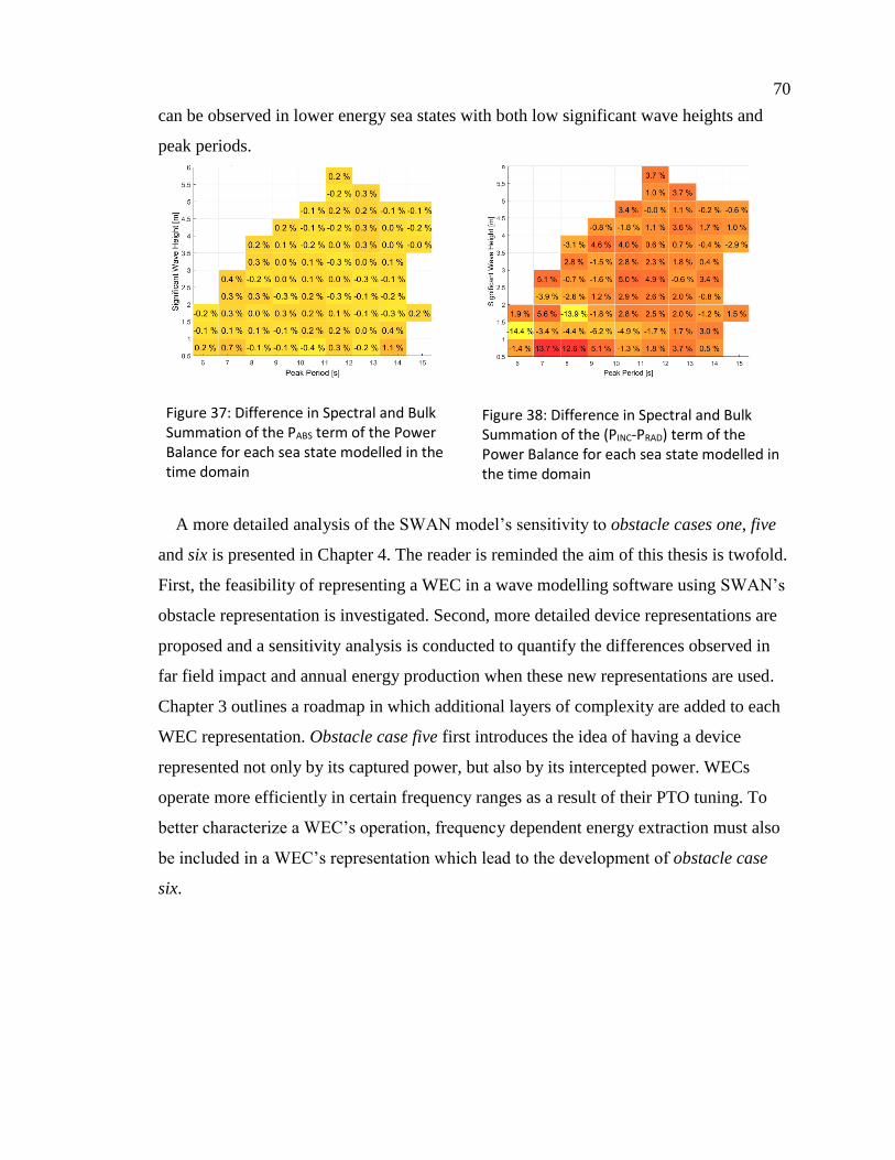
70
can be observed in lower energy sea states with both low significant wave heights and
peak periods.
Figure 37: Difference in Spectral and Bulk Summation of the PABS term of the Power Balance for each sea state modelled in the time domain
Figure 38: Difference in Spectral and Bulk Summation of the (PINC-PRAD) term of the Power Balance for each sea state modelled in the time domain
A more detailed analysis of the SWAN model’s sensitivity to obstacle cases one, five
and six is presented in Chapter 4. The reader is reminded the aim of this thesis is twofold.
First, the feasibility of representing a WEC in a wave modelling software using SWAN’s
obstacle representation is investigated. Second, more detailed device representations are
proposed and a sensitivity analysis is conducted to quantify the differences observed in
far field impact and annual energy production when these new representations are used.
Chapter 3 outlines a roadmap in which additional layers of complexity are added to each
WEC representation. Obstacle case five first introduces the idea of having a device
represented not only by its captured power, but also by its intercepted power. WECs
operate more efficiently in certain frequency ranges as a result of their PTO tuning. To
better characterize a WEC’s operation, frequency dependent energy extraction must also
be included in a WEC’s representation which lead to the development of obstacle case
six.

71
Table 4: Obstacle case summary
Obstacle User Input Transmission Dependencies
0 Ratio Constant None. 1 Power Matrix Constant Hs, Tp 2 RCW Curve Constant T 3 Power Matrix Frequency Dependent Hs, Tp
4 RCW Curve Frequency Dependent T 5.1 Power Matrix
Power Absorbed Matrix
Constant Hs, Tp
5.2 Power Matrix Incident Power Matrix Radiation Matrix
Constant Hs, Tp
6 Power Matrix Relative Capture Width Matrix
Frequency Dependent Hs, Tp, T
In total, eight representations have been proposed in Chapter 3. Certain representations
will not be analyzed any further due to a lack of input information or challenges in
implementation. Of the newly proposed device representations (obstacle cases five and
six), both representations are only investigated as sinks due to practical limitations when
investigating the performance of the reference WEC. In obstacle case five assuming an
equal distribution of radiation in front of and in the lee of the reference WEC, the WEC
removes more power than is present in the incident sea for the reference device. Obstacle
case six could also not be employed as a source and a sink because it would suffer from
cases where at particular frequencies the transmission coefficient would exceed one. This
problem stems from the device’s representation and the creative choice of using the
device’s width to normalize the power produced by the device, which will also be
discussed in Section 5.1.1. This issue is further discussed in Chapter 5. By representing
the device solely as a sink, the power radiated by the device is present only in the lee thus
reducing the net power absorbed by the device.
Obstacle case 6 is investigated also as a sink allowing the user to compare a constant
transmission representation (obstacle case 5) to a frequency dependent one. The WEC
representations investigated in Chapter 4 have been carefully chosen for their capacity to
demonstrate the defining characteristics of each representation.

72
Chapter 4
Results
Two novel representations of a WEC within a spectral action density model were
proposed in Sections 3.6 and 3.7. Both representations use time series data from high
fidelity time domain simulations to more accurately depict the device’s hydrodynamic
behaviour at sea. The author has chosen to analyze the sensitivity of the captured power
by a device and the far field impact of a device when characterized with the new obstacle
cases. It is of the highest importance to determine whether SNL-SWAN is at all sensitive
to the additional layers of fidelity. Obstacle cases five and six require more preprocessing
than cases zero through four adding to the computational expense of characterizing a
device. This chapter establishes the impact of representing a device with additional pre-
processed data.
In this chapter, the power production and far field impact of an array is compared
between obstacle cases one, five and two instances of obstacle case six. Results of the
first simulation set are presented in Section 4.1.2 in which a single device is observed in a
flat bottom domain followed by an analysis of five WECs in series. Section 4.2.3
describes the results collected from a field study at Amphitrite Bank in which the new

73
WEC representations are applied to determine the array’s far field impact at a real
location and the impact of each representation on determining an array’s annual energy
production.
4.1 Flat Bathymetry Domain Simulations
Rather than conducting a validation of the newly developed source code, a sensitivity
analysis is conducted. The previously implemented obstacle case one is compared to the
novel obstacle cases five and six. Obstacle cases two, three and four were discounted
from further analysis as the computational expense for generating the input files
surpassed any additional fidelity that could be gained from these representations, as
discussed in Section 3.8. An initial sensitivity analysis is conducted within a flat bottom
domain with an incident wave condition corresponding to the most commonly occurring
sea state at Amphitrite Bank (Hs=1.75 m, Tp =11.1 s), as described in further detail in
Section 4.1.1.
4.1.1 Flat Bathymetry Domain Description
In the first case studies, a flat bottom domain was employed in order to eliminate bias
that may result from a changing topography. By stripping away layers of complexity such
as: varying bathymetry and non-stationary boundary conditions, and neglecting non-
linear forcings, one can more clearly discern the differences imposed on the surrounding
wave field by each WEC representation. Any changes in the surrounding wave field or in
the power produced by the device can confidently be attributed to the WEC
representation opposed to other external factors. Within the flat bathymetry tests, two
device configurations were run in SNL-SWAN to demonstrate the effectiveness of
obstacle cases five and six. The first configuration examines the impact a single device
has on the surrounding wave climate. The second configuration is comprised of five
devices in series. This configuration is analyzed to both quantify the devices’
environmental footprint and to investigate the impact a device’s shadow has on a
subsequent device’s power production.

74
Both configurations were run in a Cartesian domain with a grid resolution of twenty
five meters in the x and y directions and a uniform 50 meter depth. The most commonly
occurring sea state at Amphitrite Bank, as presented in Section 1.6 is investigated for this
case study. An idealized Pierson Moskowitz spectrum characterized with an Hs, Tp and a
cos2 directional spreading was applied across the model domain in each of the test cases,
representing spectral shapes similar to the ones observed off the West Coast of
Vancouver Island [49]. Source terms typically used to represent non-linear phenomena
in SWAN such as wind growth, triad and quadruplet wave interactions were disabled for
this simulation to better demonstrate the impact the device has on the surrounding sea.
Configuration 1
In the first configuration, a device was represented with a line extending from (1215 m,
1215 m) to (1215 m, 1242 m), as depicted in Figure 39. This device was represented
using obstacle cases one, five, and six. Obstacle cases five and six were implemented
both as sinks as well as sources and sinks in a 2500 metre by 2500 metre computational
domain with a spatial resolution of 25 metres and a directional resolution of five degrees.
Figure 39: Device is represented as a line between two points in the computational domain (1215 m, 1215 m) and (1215 m, 1242 m) in SNL-SWAN.
Configuration 2
The second configuration consisted of five devices placed one behind the other. A 270
metre separation distance was chosen between each of the five devices. This distance
would provide maintenance vessels with sufficient space for operation and sufficient
distance for each device’s watch circle [108]. Secondly, Stratigaki has recommended

75
employing a separating distance of ten times the device’s width to reduce destructive
device interaction [62]. Similarly to the first configuration, the computational domain
extended 2500 metres in both the x and y direction with a spatial resolution of 25 metres
and a directional resolution of five degrees. An inset of the computational domain and the
five devices are presented in Figure 40 and node points defining the 5 WEC devices are
given in Table 5.
Figure 40: Device representation within an inset of the flat bathymetry computational domain.
Table 5: Coordinates of each of the devices employed in Configuration 2 of the flat bathymetry case study
Device number Coordinate 1 Coordinate 2
1 [770 m, 1215 m] [770 m, 1242 m]
2 [1040 m, 1215 m] [1040 m, 1242 m]
3 [1310 m, 1215 m] [1310 m, 1242 m]
4 [1580 m, 1215 m] [1580 m, 1242 m]
5 [1850 m, 1215 m] [1850 m, 1242 m]
The reader is warned that the Hs fields in Figure 41 and Figure 44 may appear
pixelated, however more finely resolved grids spatial grids may result in an artificial
banding pattern in the Hs in the lee of a device. This banding is commonly referred to as
the ‘garden sprinkler’ effect which emerges when the ratio of the directional and spatial
resolution is too low. Booji and Holthujisen suggest the width of the spectral bands in
frequency and direction should fulfill the following condition (∆𝜃 <1
𝑁 ) where N is the
distance across the computational domain expressed in number of mesh elements [84].
For the test cases used, this would imply a directional resolution of 0.01 degrees.

76
Unfortunately this criterion is impractical for the discretization of highly resolved grids,
leading to immense computational times and memory allocation issues. The developers
of SWAN have implemented correction terms to the energy balance equation in order to
reduce these effects, however caution must be exercised by the modeller to ensure the
directional bins are adequately resolved for each simulation. Previous sensitivity analyses
suggest that with higher directional resolutions, these perturbations will be removed. The
author chose to employ a directional resolution of five degrees to strike a balance
between accuracy, the reduction of numerical defects such as the garden sprinkler effect
and computational expense
4.1.2 Flat Bathymetry Domain Results
This section establishes the far field impact of a WEC and multiple WECs in series.
The change in the surrounding wave field and the incident wave spectrum at different
distances in the lee of the device are investigated. How these effects leads to changes in
power production downstream of the WEC are also examined.
Impact on the Surrounding Wave Field
Each of the obstacle case one, five and six representations impacted the surrounding
wave field to some extent. A two-dimensional plan view of the variation in Hs in the field
surrounding the single WEC is presented in Figure 41. Since the energy transport in the
wave field is proportional to Hs2, the significant wave height measure is a good metric for
gauging the magnitude of the WEC’s far field impacts. In Figure 41, obstacle cases five
and six attenuate Hs more than obstacle case one indicating that characterizing the device
interaction with the surrounding wave field with intercepted power opposed to captured
power has an input on the nearfield.
The attenuation to 90% of the incident significant wave height is analyzed in each of
the obstacle cases. In obstacle case one, an Hs of 1.6 metres is observed five metres
behind the device. In obstacle case five, the 1.6 metre Hs contour is observed 90 metres
while in obstacle case six, the Hs = 1.6 metre contour extends 70 metres behind the
device.
With respect to Hs recovery, The Hs recovers to 1.72 metres 100 metres behind the
device in obstacle case one, 330 metres behind the device in obstacle case five and 260

77
metres behind the device in obstacle case six. Of the two representations accounting for
the device’s intercepted power, obstacle case six has less of an impact on the significant
wave height in the lee of the WEC device. Obstacle case six removes power from
selected frequency bins in the wave spectrum. The incident power and radiated power are
both represented as sinks. As such, the radiated power compensates for the power
absorbed by the device since both quantities are only represented in a single direction due
to directional limitations of this particular representation, and since only certain
frequency bins are affected.
Even though obstacle case five and six remove the same amount of power from the
system, there are differences in the Hs reduction in the lee of the device when these two
representations are employed. The difference is attributed mostly to the different methods
with which the power absorbed is calculated for these two representations. The
transmission coefficient for obstacle case six is interpolated from an RCW matrix
generated with the spectrum used in ProteusDS. The total energy flux was used as
incident power opposed to the orthogonal projections of the directional power used in
obstacle case five. Secondly, the spectrum within ProteusDS had 20 frequency bins and
seven directional bins. When SNL-SWAN calculates the transmission coefficient it must
linearly interpolate from a set of half the bins Depending on how peaked the RCW curve
is, this interpolation can cause underpredictions in power as well.
The Hs contours in each of the obstacle cases are roughly circular, increasing in area as
greater decreases in Hs are observed directly behind the device. The circular pattern can
be attributed to the fact that the transmission coefficients are insensitive to direction.
These circular patterns are likely to change if directionally dependent transmission
coefficients are implemented in future WEC representations in SNL-SWAN.
Additionally, the transmission coefficient in obstacle case five was determined from the
perpendicular projection of the incident spectrum onto the device’s inlet. If the waves
were to come from an oblique incidence angle, the magnitude of energy perpendicular to
the device would decrease, reducing the denominator in Eq. (14), increasing the
transmission coefficient.

78
Figure 41: Significant wave height comparison demonstrating a device's impact on the surrounding wave field when represented with different obstacle cases in the most commonly occuring sea state off of Amphitrite Bank (Hs=1.75 m, Tp = 11.1 s)
The difference between these representations becomes even more apparent when the
wave spectra in the lee of the device are studied. Figure 42 presents the omni-directional
variance spectra interpolated at five metres (top left), 25 metres (top right), 100 metres
(bottom left) and 200 metres (bottom right) behind the device. This figure demonstrates
both how the variance spectrum recovers as it moves further away from the device as
well as how the device removes energy from the variance spectrum depending on its
representation. The wave spectrum incident to the device is presented in black for
reference.

79
Figure 42: Comparison of non-directional variance density spectra at various distances behind the WEC when the WEC is represented with obstacle cases one, five and six.
The greatest decrease in variance can be observed directly in the lee of the device, as
can be seen in the top left corner of Figure 42. The variance spectra modified by obstacle
cases one and five are scaled forms of the incident variance spectrum. The uniform
decrease in the spectrum is expected given a frequency independent transmission
coefficient is applied in both cases. The spectrum corresponding to obstacle case six has
been non-uniformly decreased as a function of frequency as can be seen in the relative
capture width curve presented for this sea state in Figure 31. Obstacle case six removes
the most power at the spectrum’s peak (0.09 Hz)as well as to the right of the peak (0.11
Hz), where the device operates most efficiently [20].
At a distance of 25 metres behind the device (top right), the variance density spectrum
is seen to recover quickly. One may also observe that the variance density spectra
affected by the frequency dependent representations of the device have shifted variance
back into the peak frequencies resulting in a spectrum that more closely resembles the
incident Pierson Moskowitz spectrum. The device representations that removed less

80
energy from the incident wave spectrum recover at a slower rate than those that removed
more. As one moves further from the device, at 100 metres (bottom left), all spectra have
assumed the same shape with differences in amplitude depending on the representation.
Finally, at 200 metres away from the device (bottom right), the spectra have all nearly
recovered to the same levels of variance, across all frequencies, as the inlet spectrum.
An additional analysis was conducted in which the non-directional variance density
spectrum was analyzed for each WEC representation at different distances from the
device as seen in Figure 43.
Figure 43: Evolution of variance density spectrum with increasing distance away from the WEC when the WEC is represented with different obstacle cases.

81
This view is intended to give a clear visualization of the recovery of the wave spectrum
in the lee of the converter. In all device representations, the variance spectrum recovers as
the variance spectrum propagates further from the device. This growth in variance can be
attributed to energy transport diffracting around the obstacle and moving into areas of
lower energy in the lee of the device. The frequency dependent energy extraction in
obstacle case six is most prominently observed five metres behind the device. The
spectrum assumes a shape similar to that of the incident spectrum 50 metres behind the
device. As previously mentioned in the discussion of Figure 42, obstacle case six
removes the most energy at the spectrum’s peak as this is the frequency at which the
device operates most efficiently.
Figure 44 presents a surface plot depicting the modification of Hs when five devices are
placed in series at a spacing of ten device widths.
Figure 44: Hs contours surrounding a line of five devices spaced 10 device widths away from one another
The top plot of Figure 44 corresponding to the wave field around a device represented
with obstacle case one. The middle and bottom plots show analogous results from when
obstacle cases five and six are run. The first device maintains a narrow elliptical
significant wave height contour, which grows in width after each subsequent device. In
addition, one may observe a greater decreases in Hs closer to the device’s node points
opposed to directly behind the device. The decrease in significant wave height near the
obstacle’s node points can be attributed to diffraction around the device. As energy

82
diffracts in from both sides of the device it concentrates directly in the lee of the device
as a result of the incident spectrum’s directional spread. A directional spread of two was
run as this corresponds to the directional spread employed in the time domain
simulations. The same pattern is observed in each obstacle case, with differences in the
magnitude and spatial extent of the Hs attenuation.
The recovery of Hs directly in the lee of five devices is presented in Figure 45. All
device representations result in a similar pattern in Hs profile. Obstacle case five
consistently reduces the significant wave height more than obstacle case six. At first the
difference is merely 0.02 metres between the two, and by the fifth device the difference
in significant wave height reduction increases to 0.04 metres. The incident Hs at each
device is presented in Table 6. Small differences in Hs are observed at the last three
devices. As the incident Hs decreases, a greater transmission coefficient is employed for
this particular sea state, thus reducing the power absorbed at each device.
Figure 45: Comparison of the profile view of the Hs and its recovery in the lee of five devices when the devices are represented with different obstacle cases

83
Table 6: Hs incident to each device, when devices are represented with obstacle cases one, five and six.
Device number Obstacle Case One Obstacle Case Five Obstacle Case Six
1 1.750 1.750 1.750
2 1.739 1.713 1.720
3 1.734 1.700 1.710
4 1.731 1.694 1.705
5 1.729 1.690 1.702
Figure 46: Cross sections of the Hs profile 100 metres behind each device when using different obstacle case representations.

84
As presented in Table 6, the wave height incident to the last device is decreased by 1.2%
when obstacle case one is employed, 3.4% when obstacle case five is employed and
2.7% obstacle case six is employed
Finally, a cross-sectional view of the Hs 100 metres behind each of the five devices is
presented in Figure 44. In each of the section views, there is a sharp jump between 1200
metres and 1225 metres, as well as between 1225 and 1250 metres. This jump is largely a
result of interpolation and would not be present if a higher spatial resolution was
employed. Due to the garden sprinkler effect discussed in Section 4.1.1, a higher spatial
resolution would also create artificial oscillations in Hs across the Hs profile. Obstacle
cases five and six recover at similar rates behind each device along the cross sections. The
greatest difference between the first device’s significant wave height profile and the last
device’s significant wave height profile is seen when employing obstacle case five.
Impact on power production
The representation used for a WEC also impacts the power production of each device.
Each device decreases the Hs in the device’s lee, ultimately changing the incident
conditions of the subsequent device until a steady state is reached in which the conditions
no longer change for each device thereafter.
Given each representation modifies the surrounding wave field to a different degree,
the power captured by a device from the incident wave field will also change with each
representation. The power produced by each of the five devices in the second
configuration is reported in Table 7 followed by the percentage decrease in captured
power presented in Table 8. The percentage decrease is calculated by comparing each
individual device’s captured power to that of the first device in obstacle case one, five
and six. The greatest decrease is observed in obstacle case five, as in this representation
the device absorbs the most power. At each subsequent device however, the power
captured stays quite similar ranging between five and six percent of the first device’s
power capture. In obstacle case one, the reduction in power capture for each subsequent
device ranges between 1.5 and 2.5% of the first device’s power capture and finally in
obstacle case six, the decrease in captured power ranges between 3.5 and 4.5% indicating
relatively small losses in power when devices are spaced ten device widths apart.

85
Table 7: Captured power [kW] produced by five devices placed ten device widths behind the previous for each obstacle case
Captured Power [kW] for each device in series
Obstacle case 1 2 3 4 5
1 88.50 87.13 86.69 86.52 86.45
5 88.50 83.79 83.39 83.35 83.34
6 88.50 85.23 84.91 84.82 84.79
Table 8: Percentage decrease in captured power produced by five devices placed ten device widths behind the previous for each obstacle case
Percentage decrease [%] in captured power
Obstacle case 1 2 3 4 5
1 0 1.54 2.05 2.24 2.32
5 0 5.32 5.77 5.82 5.83
6 0 3.69 4.06 4.16 4.19
Even though this test case was carried out for a single sea state, previous analyses have
indicated applying the obstacle case five representation will result in an average 5.7%
decrease between power produced by the first and second device when averaged over
each sea state that occurred at the field case location in 2006 [109]. The shadowed device
has been observed to produce as much as 9.8% less power than the first device in series
in higher energy seas [109].
The results presented in this section are specific to the reference device and the device
spacing chosen and as such, caution should be exercised in generalizing these results.
4.2 Field study: Amphitrite Bank
In this section, a case study is presented in which an array of fifty four devices is
modelled six kilometres off the coast of Amphitrite Bank to meet the load requirements
previously outlined by the local electrical utility [110]. Amphitrite Bank has been
identified by the local power authority, BC Hydro, as a promising location for a WEC
array due to its proximity to major grid interconnections at the community of Ucluelet,
suitable bathymetry and a strong wave energy resource [110], [111]. The site was also
identified as a promising WEC farm location in previous studies of the gross wave
resource off the West Coast of Vancouver Island [55], [112].

86
4.2.1 Field Simulation Description
Three nested SWAN simulations were used to create the 54 unit WEC array model at
Amphitrite Bank. Nested simulations use a larger spatial grid to generate boundary
conditions at the boundaries of a smaller, higher resolution computational domain. Three
domains were employed (two of which being nested grids) to allow for flexibility in
generating the final domain in which the WEC array is placed. By employing an
intermediate grid, the user can avoid running a SWAN simulation of a large,
computationally expensive domain if changes are made to the orientation of the smallest
grid. The structure of the nested runs and the inputs are displayed in Figure 47 followed
by a more detailed description of each of the computational domains.
Figure 47: Nesting structure of the field case model for a farm of 50 devices
A pre-existing SWAN grid formerly used to characterize the wave resource off the
West Coast of Vancouver Island (WCVI) [42] was used to determine the boundary
conditions for subsequent simulations. Within the WCVI grid, the depth ranges from
approximately 1000 metres at the continental shelf to zero depth at shore [55]. An
unstructured computational grid for the WCVI region was generated using the grid

87
generation software TQGG17 Unstructured grids allow for greater computational
efficiency and improved resolution for wave effects in shallower regions. Grid spacing
was specified proportional to water depth with the most highly resolved elements 50
metres in length. The bathymetry was interpolated onto the computational grid from
500m and 100m gridded bathymetry sets from the Canadian Hydrographic Service [42].
The grid covers over 410,000 square kilometres with over 130,000 computational nodes.
Figure 48: West Coast of Vancouver Island (WCVI) grid from which the boundary conditions of subsequent simulations are extracted. The surface presents the average Hs over the duration of the 2004-2013 Hindcast
Wave boundary conditions from the WCVI grid were obtained from an ocean-scale
wind-wave model (WAM) operated by the European Centre for Medium Range Weather
(ECMWF). Wind boundary conditions were gathered from the Coupled Ocean/
Atmosphere Mesoscale Prediction System (COAMPS) model developed by the U.S.
Navy. The large WCVI grid was run with boundary conditions obtained from FNMOC
17 https://github.com/rrusk/TQGG

88
WW3 for all of 2006 at a three hour resolution. Spectral data was output at the boundary
nodes for the subsequent grid.
A higher resolution grid, shown in Figure 49, was generated off the coast of Ucluelet
using the bathymetry files from the larger WCVI SWAN grid. The Ucluelet grid extends
30 kilometres off shore at the northern boundary and 53 kilometres offshore at the
southern boundary of the grid. The Ucluelet grid is 110 kilometres in length with the
lowest resolution at the offshore boundary where cell edges are 1.5 kilometres in length
and the highest resolution near the coastline where cell edges are 200 metres in length.
The Ucluelet grid contains 3571 nodes and 6693 cells.
Figure 49: On the left, the unstructured grid used in the WCVI map is superposed onto the physical map of the Amphitrite Bank. On the right, the computational grid as run in SNL-SWAN is presented for the area indicated by the red outline on the left figure. Bathymetry is indicated by the color scale on the right. All depths are in metres.
Finally, a regular, structured Wave Farm grid was generated within the Ucluelet grid
with the bottom left corner located at a longitude and latitude of 234.4 and 48.76 degrees
respectively corresponding to an area of higher wave energy as seen in Figure 51. The
Wave Farm grid has a 25 metre resolution in both the x and y directions and 630,000
nodes. A structured grid was employed to reduce numerical error diffusion that occurs in
very fine unstructured grids. The x-axis is aligned with the principle wave direction with
the y-axis perpendicular to it. The Wave Farm grid was angled at 80 degrees to be
aligned with the mean annual wave direction (260 degrees) averaged over the duration of
the hindcast between 2004 and 2013, as seen in Figure 50. The Wave Farm grid extends
20 kilometres along the x dimension of the grid and 28 kilometres in the y direction. It

89
should be noted that the regular Wave Farm grid is rectangular in Cartesian coordinates
and takes on the shape of a skewed polygon when translated into latitude and longitude.
The regular grid is the most resolved of the nested grids and is the grid on in which the
wave farm constructed using SWAN’s obstacle feature.
Figure 50: Map depicting the depth contours across the Ucluelet grid and the mean wave direction across the site averaged over 2004-2013
Figure 51: Map depicting the wave energy transport across the Ucluelet grid averaged over the years 2004-2013

90
4.2.2 Array Format
The array configuration used within this analysis was influenced by array spacing
configurations previously suggested by Stratigaki [62] as well as practical electrical
transmission considerations reported by MacArtney [113]. Devices were spaced at ten
device widths in smaller subarrays of nine devices. Stratigaki recommends the
installation of WECs in smaller arrays with at least a ten device diameter spacing
between devices to limit far field impacts and reduce intra-array interactions between
devices. Stratigaki reported a constructive effect of intra-array interactions for 3 x 3
arrays spaced ten device widths apart when experimentally testing arrays in long crested
irregular waves [62]. The constructive interactions between these devices were decreased
when 5 x 5 arrays were tested. It should be noted that even with constructive interaction
between WECs, the devices on average performed less efficiently in an array than when
individually deployed. Smaller subarrays of devices are also compatible with the
recommended electrical infrastructure configuration previously suggested by the
MacArtney Group [113]. The MacArtney study was focussed on the conceptual design
of the subsea electrical infrastructure required for a WEC array installation on Amphitrite
Bank. Components of the electrical system were drawn from MacArtney’s established
products used in offshore wind energy applications. Modular hubs are used to connect
and combine inputs from multiple dynamic cables connected to individual WECs and
export the power.
Figure 52: Diagram presenting one device connected to a modular hub [113]

91
In practice, the number of connections to the hub is limited by the electrical rating of
the export cable, which necessitates the need of smaller arrays. MacArtney’s study
concluded with a 54 device layout within which three devices are connected to each
modular hub in smaller arrays of nine devices [113].
Figure 53: Position of 54 WEC devices presented within in the computational domain superposed on the domain's depth
4.2.3 Field Case Results
The computational domain presented in Figure 53 was modelled with boundary wave
conditions in 2006 with a three hour time step. The boundary conditions were determined
based on the nesting procedure outlined in Figure 47. The WCVI grid was run for 2006.
This model run saved boundary conditions at nodepoints corresponding to the Ucluelet
grid’s boundary nodes for the duration of the year. The Ucluelet grid was then evaluated
with the previous simulation’s outputs and the outlined procedure was repeated for the
Regular Wave Farm grid boundary conditions.
In order to compare the performance of obstacle case one, five and six with respect to
annual energy production and far field impact, four chief model outputs were recorded
from the simulations. First, the power captured by each WEC was recorded for each time
step in the simulation. Second, the Hs, Tp, peak direction and energy transport, from

92
herein collectively referred to as bulk parameters, were recorded for each node
surrounding the WEC array, as can be observed in Figure 57 through Figure 62. The bulk
parameters at these field points are used to visualize the interaction between devices
within the farm, ultimately allowing one to understand why certain changes in power
production may occur between the devices. The bulk parameters were interpolated at
cross sections through the Wave Farm grid at 100, 200, 500, 1000 metres behind the
array and also at a location close to the shoreline in order to determine the far field
impact the WEC array has on the very near shore region. These cross sections are
presented in Figure 54.
Figure 54: Location of the far field impact lines, as located behind the array of 54 WECs superposed on a depth plot for a section of the computational domain.
The simulations conducted for this work required 3774 hours of CPU time and were
run in both series and parallel on five machines each with 16 cores. Simulations run with
obstacle case five required more CPU time than obstacle cases one and six. The author
presumes this is due to the large decreases in Hs incurred with representing a device with
obstacle case five. As a result, SWAN needs to iterate more for each time step in order to
find a solution that meets the user’s convergence criteria set in the input file.
The remainder of this section is split into two primary parts. First, the impact the WEC
array has on the surrounding wave field – both with respect to far field and intra-array
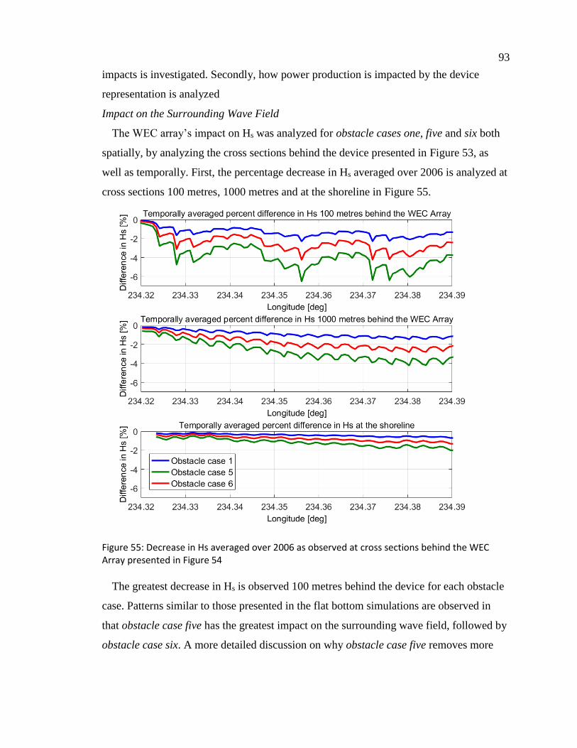
93
impacts is investigated. Secondly, how power production is impacted by the device
representation is analyzed
Impact on the Surrounding Wave Field
The WEC array’s impact on Hs was analyzed for obstacle cases one, five and six both
spatially, by analyzing the cross sections behind the device presented in Figure 53, as
well as temporally. First, the percentage decrease in Hs averaged over 2006 is analyzed at
cross sections 100 metres, 1000 metres and at the shoreline in Figure 55.
Figure 55: Decrease in Hs averaged over 2006 as observed at cross sections behind the WEC Array presented in Figure 54
The greatest decrease in Hs is observed 100 metres behind the device for each obstacle
case. Patterns similar to those presented in the flat bottom simulations are observed in
that obstacle case five has the greatest impact on the surrounding wave field, followed by
obstacle case six. A more detailed discussion on why obstacle case five removes more

94
power than six was previously presented in Section 4.1.2. The mean percentage decreases
in Hs behind the array at the cross sections presented in Figure 54 is presented in Table 9.
As a result of the mean wave energy transport approaching the farm from the west over
most of the year, the greatest decrease in Hs is observed behind the devices near the
eastern extent of the array. The computational grid was angled according to the mean
wave direction over the duration of the 2004-2013 hindcast however in 2006, the waves
approached Amphitrite Bank more from the west. The author anticipates if the grid were
angled to the dominant wave direction, there would be a horizontal, averaged wake
behind the array. In the top plot of Figure 55, the reader may also observe a greater
decrease in Hs at longitudes 234.328 and 234. 356. These coordinates correspond to
where two adjacent 3 x 3 arrays meet. The impact of the two neighbouring arrays is no
longer observed 1000 metres behind the device, however the eastern extent of the array
remains more affected by the presence of the array. Finally, near the shoreline, regardless
of the obstacle case employed, less than a two percent decrease in Hs is observed.
Table 9: Temporally and spatially averaged difference in Hs observed at the specified distances for each device representation.
Distance from Array [metres]
Obstacle case 100 200 500 1000 Shoreline
1 -1.34 -1.27 -0.95 -0.63 -0.44
5 -3.86 -3.66 -2.79 -1.87 -1.27
6 -2.46 -2.34 -1.83 -1.26 -0.84
In addition to the average difference in Hs observed over the course of a representative
year, it is important to consider the condition which would decrease the Hs most.
Significant wave height cross sections corresponding to December 6, 2006 at 18:00 are
presented in Figure 56. This time step corresponds to when obstacle case five removed
the most energy from the WEC array in 2006. At this time step, the mean energy
transport direction is coming from the east creating a more prominent decrease near the
eastern extent of the WEC array. The greatest decrease across the 100 metre cross section
approaches a 15% decrease in Hs when obstacle case five is employed. Even when the far
field impact is deemed the worst, the reduction in Hs at the shoreline is observed to be
less than 5% regardless of the representation used for the WEC array. The cross sections

95
at which the significant wave height was recorded are presented in Figure 54. A more
detailed list of Hs decreases for each of the obstacle cases is presented in Table 12.
Table 10: Spatially averaged difference in Hs observed on December 6, 2006 at the specified distances for each device representation.
Distance from Array [metres]
Obstacle case 100 200 500 1000 Shoreline
1 -2.26 -2.17 -1.72 -1.10 -0.57
5 -7.57 -7.23 -5.67 -3.54 -1.80
6 -4.38 -4.15 -3.09 -1.71 -0.72
Figure 56: Decrease in Hs observed at the cross section behind the WEC Array, as presented in Figure 54 on December 6, 2006 at 18:00 hrs
In addition to the impact the farm has on Hs, bulk parameters are analyzed within the
vicinity of the WEC array. Figure 57 through Figure 59 present the Hs, direction of the
energy transport, peak direction and the Tp in the wave field surrounding the farm in the

96
most commonly occurring sea state in 2006. Figure 60 through Figure 62 present the
same bulk parameters for a higher energy sea, demonstrating how the device behaviour is
impacted by the WEC representation in more extreme conditions defined in Table 11.

97
Figure 57: Bulk Parameters plotted across the WEC farm for the most commonly occurring sea state when devices represented with obstacle case one

98
Figure 58: Bulk Parameters plotted across the WEC farm for the most commonly occurring sea state when devices represented with obstacle case five

99
Figure 59: Bulk Parameters plotted across the WEC farm for the most commonly occurring sea state when devices represented with obstacle case six

100
Figure 60: Bulk Parameters plotted across the WEC farm for a high energy sea (Hs = 4.75 m, Tp = 13.5 s) when devices represented with obstacle case one

101
Figure 61: Bulk Parameters plotted across the WEC farm for a high energy sea (Hs = 4.75 m, Tp = 10.5 s) when devices represented with obstacle case five

102
Figure 62: Bulk Parameters plotted across the WEC farm for a high energy sea (Hs = 4.75 m, Tp = 10.5 s) when devices represented with obstacle case six

103
Table 11: Description of wave conditions under which obstacle cases one, five and six were analyzed for the field case
Description Hs [m] Tp [s]
Commonly occurring 1.75 11.1
High Energy 4.75 13.5
In the most commonly occurring sea state, the greatest difference between the three
device representations is observed in the Hs. field. The Hs is most prominently decreased
in the lee of the fifth 3 x 3 array from the left. Because the energy transport is
approaching the WEC array from the east (as seen in the top right plot of Figure 60
through Figure 62), the energy spectrum incident to the WEC array has already been
perturbed by the second and fourth 3 x3 array. The change in Hs in the lee of the device at
100, 250 and 1000 metres is presented in Figure 63 below. The reader may also note that
when the energy transport is directed perpendicular to the array the decrease in Hs is more
uniform across the width of the array.
Figure 63: Hs interpolated at 100, 250 and 100 metres in the most commonly occurring sea state in 2006

104
The peak direction of the waves propagating across the WEC farm are influenced by
the WEC representation to a lesser degree. In Figure 57, the peak direction surrounding
the fourth, sixth and part of the fifth array is 285 degrees. At a closer glance, directly in
the lee of certain devices in the second and third array, there are also pockets of 285
degree peak direction. When obstacle case five is employed, additional pockets of 285
degree peak directions manifest themselves around devices in the corner of the second
array from the left. This effect is very small because this is not a very high energy sea.
The peak period is relatively unaffected by the device representation in an Hs = 1.75
metre and Tp = 11.1 second sea. If one looks closely at the peak period plot in Figure 59,
the peak period jumps to 12.4 seconds directly in the lee of each of the devices
characterized with obstacle case six. It appears that in this particular sea state, most of the
energy was extracted from the peak of the incident energy spectrum. As a result, a new
peak was created. Because of the directional spread of the incoming waves, and as these
waves diffract around the device, the spectrum assumed its original shape as it travels
further from the device. This phenomenon was also seen in Figure 42 when the spectrum
behind a single device was observed. The author believe that a more continuous variation
in the mean period would be seen across the computational domain however, the peak
period was analyzed as it is used to determine the power absorbed by the device from the
power matrix.
More prominent changes in the wave field can be observed when the three obstacle
cases are observed in a higher energy sea state, such as the one presented in Figure 60
through Figure 62. Similarly to the lower energy sea, the greatest decrease in Hs can be
observed in Figure 61 corresponding to obstacle case five. The first, third and fifth array
undergo the greatest decrease in Hs, as their wave field is partially shadowed by the first,
third and fifth arrays. This effect is presented more clearly in Figure 64 where there are
greater dips in the Hs directly in the lee of the first, third and fifth arrays for each of the
obstacle case. At 250 metres behind the device, the array configuration’s impact on the
Hs profile is still observed while at 1000 metres, the decrease in Hs is uniform along the
length of the array.

105
Figure 64: Hs interpolated at 100, 250 and 100 metres in a high energy sea
The direction of the energy transport remains unaffected between the three obstacle
cases. The peak direction plot however demonstrates how each obstacle case impacts the
peak direction within the array. In obstacle case one, a small pocket of waves is observed
where the peak direction is 155 degrees, opposed to the incoming waves which range
between 255 and 275 degrees. The peak direction is most drastically changed in obstacle
case five. It is believed that the devices are extracting so much power from the incident
component of the energy transport projection that the peak direction of the energy
spectrum begins to change. This hypothesis is supported by the fact that the peak
direction is reduced to a value that’s roughly perpendicular to 255 degrees.
The peak period is also impacted by the device representation. In Figure 60, the peak
period changes across the WEC farm as a result of a storm approaching the farm. An
increase in Hs can also be observed along the same front in the top left plot of Figure 60.
In Figure 61 and Figure 62, this change in peak period is observed further across the
farm, most prominently directly in the lee of the devices on the western extent of the
farm.

106
Field Case Annual Energy Production
The different representations used to model the WEC array on Amphitrite Bank
impacted the assessment of power production. Over the course of a year, the different
representations employed to characterise a WEC array installed off of Amphitrite Bank
resulted in a mean percentage decrease in power of 3.8% when obstacle case one was
compared with obstacle case five, and a mean percentage decrease of 2.7% when
obstacle case six and obstacle case one were compared, as stated in Table 12, indicating
that including hydrodynamic losses does influence the power produced by a WEC array,
even at a ten device width spacing where the incident energy spectrum has almost fully
recovered, as was seen in Figure 42.
Table 12: Annual Energy Production for a Farm of 54 devices deployed off of Amphitrite Bank in 2006 when represented with three different representations in SNL-SWAN
Obstacle case Annual Energy
Production (GWh) Percentage Difference
1 47.4 0
5 46.0 -2.9
6 46.3 -2.3
On aggregate, including the intercepted power in the device representation reduces the
mean farm power production by less than five percent. However, the performance of an
individual device in an array is more drastically affected. To gain a better appreciation for
how a device’s power production can change temporally, the difference in power
production for a device is presented in Figure 55. One may observe that on average
obstacle cases five and six remove more power from the incident sea than obstacle case
one however there are instances when the intercepted power representations will
suddenly produce much more, or much less power (as depicted by the spikes in power
production) because of a local shift in Tp. The line is discontinuous in the bottom plot of
Figure 65 where no power is being produced by any of the devices.

107
Figure 65: Time Series of the captured power by a device in the first row of the first array in January 2006 (top). The difference in power produced by a device using when comparing between different obstacle cases and the baseline (obstacle case one)
Figure 66 presents the percentage difference in annual energy production (AEP) for
each device in the array to the reference representation (obstacle case one). The greatest
decrease in power production when employing obstacle case five is observed in the
eastern most device in the fifth array from the left. An 8.1% decrease in captured power
is observed largely due to the fact that this device is the most shadowed over the course
of the year. The same trend is observed when obstacle case six is analyzed.
Even though obstacle case five and six should theoretically remove the same amount of
power from the incident wave spectrum, the RCW matrix generated for obstacle case six
assumed a Pierson Moskowitz spectrum when normalizing the power absorbed by the

108
device. If the spectrum incident to the farm has a different shape, the transmission
coefficients derived may be applied to bins containing different magnitudes of energy
density than assumed in the preprocessing step. Because obstacle case five reduces the
incoming spectrum by a constant transmission coefficient, this representation is less
sensitive to spectral shape and appears to remove more energy from the incident sea.
Figure 66: Percentage difference in annual energy production between obstacle cases one and five (top) and one and six (bottom)
It is also interesting to note that there is a decrease in captured power in the first row of
devices in the array for both obstacle cases five and six as seen in Figure 66. The author
believes this phenomenon is caused by wave directions coming from 180 degrees during
some instances over the course of the year. Devices closer to the western extent of the
array are shadowed by those located further east and by extension produce less power
over the course of the year.
Comparing the annual energy production of the array when represented with different
obstacle cases is subject to significant smoothing over the different incident wave
directions and amplitudes experienced by the WEC array. Figure 67 compares the power
produced by each device in obstacle case five and six in the most commonly occurring

109
sea previously presented in Figure 57 through Figure 59. Because the energy transport
was coming from the east, the greatest reduction in power is observed in the western most
devices. In a real field case, another potential source of error comes to light. Obstacle
case six has transmission coefficients assigned to particular bins assuming that the
incident spectrum was a Pierson-Moskowitz spectrum with a cosine squared directional
spread. In this field case, there may be real spectra that may not resemble the reference
spectrum, causing the same transmission coefficient to be applied to a different amplitude
of incident power.
Figure 67: Percentage difference in power produced between obstacle cases one and five (top) and one and six (bottom) for the most commonly occurring sea
The difference in power production is also compared between obstacle cases five and six
for a higher energy sea in Figure 68. This case is particularly interesting because the
devices on the eastern flank of the WEC array produce more power in obstacle case five
than in one. In obstacle case five, the reduction in Hs by the first row of device in the
fourth, fifth and sixth 3 x 3 arrays decrease the Hs to such an extent that a higher power
production value is being interpolated for the devices in the lee. A similar phenomenon is

110
observed when one compares obstacle case six and obstacle case one. On the western
flank, once again, another bin is being referenced in the captured power matrix. One may
observe in Figure 62 that the peak period is 13.56 s for almost the entire array while this
is only the incoming condition on the right in Figure 60. The difference in peak period,
combined with the decrease in Hs in the lee of the first row of devices change the incident
condition to the shadowed devices.
The results presented are subject to a spacing that was set to ten times the device width
and an array layout that was trying to minimize interference which is subject to change if
another configuration is employed by the user. The results lend hope that a second row of
54 devices could be built behind the current one and still perform quite well. The
performance of this second row will depend on how the devices are represented and as
such we may see accumulating differences in the estimates made using obstacle cases
one, five and six in that case
Figure 68: Percentage difference in power produced between obstacle cases one and five (top) and one and six (bottom) for the higher energy sea

111
Chapter 5
Unresolved issues
Over the time the author has spent working to improve the representation of a WEC
device in SNL-SWAN, certain limitations imposed by the structure of the existing SNL-
SWAN source code have been revealed. Some of these limitations are inherent to the
device’s representation as an ‘obstacle’ in SWAN, some stem from the finite set of time
domain simulations used to populate the representation and some arise from practical
limits made to keep the computational expense of the proposed methodology low.
This chapter is divided into three parts. Section 5.1.1 describes physical limitations
imposed by the way the obstacle is applied within the finite difference solution of a
spectral action density balance. Section 5.2 lists assumptions and approximations made
within the time domain model which can lead to an inaccurate representation of the
device. Finally, Section 5.3 identifies systematic error that occurs in the post processing
of the time domain data and finally Section 6 presents the need to validate the work
presented.

112
5.1 Device Representation in SWAN
Representing a device as an obstacle was a convenient and natural first step when
trying to include a WEC in a coastal model however, as with any simplification,
limitations exist to this approach. This section outlines issues associated with the
geometric representation of a device within SWAN and the representation of the radiation
within the model.
5.1.1 Geometric Representation
In SWAN, the location of an obstacle is defined by a sequence of node points used to
represent line segments. These lines cross a grid linkage between two nodes and interrupt
the transmission of energy density across that grid linkage.
Representing a dynamic device with a line may appear over-simplistic until one
considers the spatial and temporal scales across which SWAN operates. Inherent issues
with the representation exist, where a line cannot effectively extract power from a
directional sea. To complicate matters further, it is difficult to find a universal
representation for a device given the ever growing number of device architectures. En
masse, devices rarely resemble lines making this geometric simplification not only
visually inaccurate, but also a source of trouble when calculating a transmission
coefficient. The reference WEC in this work has a well-defined inlet and outlet but
devices which extract power from omnidirectional seas, such as the point absorber
presented in Figure 1 are more difficult to represent.
Additionally, the WEC device’s physical width is used to calculate the width of the
incoming wave front as presented in Eq. (14). Following existing SNL-SWAN
convention, the entries in an input power matrix are normalized by a capture width. Using
a device’s physical width in the calculation of RCW is a creative choice and one that has
been widely used in the WEC industry based on the perception that a WEC only interacts
with the incident wave front that it physically touches. However, this notion is
is problematic as described by Falnes and Hals:
“Quite often, results have, traditionally, been expressed by quantities as
‘absorption width’ and ‘capture width’, which have dimension length (SI unit

113
metre), or by dimensionless quantities, such as ‘capture width ratio’ and
‘(hydrodynamic) efficiency’… These technical terms focus on one horizontal
dimension (in the direction of the incident wavefront). However, a WEC has two
horizontal dimensions, in addition to a vertical one. [114]”
Devices interact with the oscillations of the surroundings waves over these other
dimensions as well. In fact, when the diffracted wave field is considered, the device is
known to perturb the surrounding wave field over a broader domain than its own physical
dimensions. Previous literature has indicated certain device architectures can absorb more
wave power than is available directly incident to the width of the device. Early
experimentation with point absorbers demonstrated devices absorbing more energy than
was directly incident to the device [115].
To summarize the issue, the power incident to the device’s primary interface is
underestimated as a result of the width chosen with which to normalize the device’s
power production. As such, when the energy density is gathered at a node point (or
lumped) it is gathered from a surrounding region that is no larger than the width of the
grid spacing it intersects. When the obstacle then removes energy during the transport
from one node to the next, the power in the incident sea is integrated over the width of
the physical device. The proposed correction is that the width needs to represent the
effective width of the device, or the device needs to be represented using another
dimension, as will be discussed in Chapter 6.
The theoretical issues presented extend into the work presented in this thesis as well.
The device’s representation has an influence on how the waver power transport across the
directional domain is modified. SWAN isolates the inlet wave spectrum to the power
crossing the line based on projections of the energy transport. When the device is
simulated in the time domain, even though the incident wave spectrum is propagated
towards the device from a principal wave direction. The incident wave forcing is
integrated across the device’s three-dimensional mesh allowing the device to be excited
not only across the face directly incident to the wave, but also along its other edges,
which is partially responsible for the difference in power absorption when the device is
represented with obstacle case five versus obstacle case six.

114
5.1.2 Representation of Radiation
Radiation can theoretically be distributed across either side of the line representing the
device in SWAN given more power is not taken out of the system than is incident. If
energy is to be conserved within the computational domain, the following condition must
be true:
𝐸𝑟 + 𝐸𝑡 + 𝐸𝑎 = 𝐸𝑖𝑛𝑐 (35)
where 𝐸𝑟 is the energy radiated by the device, 𝐸𝑡 is the energy transmitted past the
device, 𝐸𝑎 is the energy absorbed by the device and 𝐸𝑖𝑛𝑐 is the energy incident to the
device. From the power balance presented in Section 3.5, one can determine the time
averaged power absorbed, radiated and incident to the device. When the device is
represented as both a source and sink the representation of energy transmitted (leaving
through the lee of the device) and energy reflected (leaving through the front of the
device), are linked through Eq. (30). In addition to the overarching energy conservation
condition, the user must also comply to Eq. (32) to ensure that within the finite difference
scheme used in SWAN, more energy is also not taken out of the system. With the present
uncertainty in device capture width this condition could not be implemented without
violating Eq. (32) however modelling another device, or increasing the device’s width in
SWAN can make this representation a feasible alternative.
The inconsistency in representing a device as a line in SWAN is already apparent when
considering the incident loading alone. The magnitude of this problem is amplified when
considering the radiated wave. A moving device will radiate waves in all directions. The
only directional data provided by the time domain simulator is the magnitude of forces
exerted in each DOF which does not provide sufficient information to discern the
direction in which the radiated power is being transferred and the user has no knowledge
of what the radiation pattern would look like. Even with this information available,
within SWAN, the user can only propagate energy directly in front of or behind the
device as there are only two sides of a line.
The right hand plot in Figure 69 demonstrates how both the incident and radiated
power exceed the power within the incident wave spectrum at frequencies near the
spectral peak. For the simulations pertaining to the reference WEC, the power absorbed

115
by the device was calculated by taking the difference of the incident and radiated power,
as presented by the blue line in the plot on the left. Even though the author has created a
method with which the device can be characterized as both a source and a sink, this
technique is rendered moot by the fact that power must be radiated to the lee in order to
prevent the energy extraction in spectral bins to avoid saturating. Once saturated, the
energy extracted must be redistributed following the method of Section 3.7.1.3 which
adds another layer of creative modeling.
Theoretically, if a capture width greater than that of the device’s physical width was
selected, the incident wave spectrum would be scaled up allowing for more power to be
intercepted. To the author’s knowledge, there has been no method established to date
which can be used to determine the width of the wave front from which the device
intercepts power.
Figure 69: The incident wave spectrum and the power absorbed by the Reference WEC in an Hs = 1.75 m and Tp = 11.6 s sea state. On the left, the power absorbed by the device is superposed on the incident wave spectrum. On the right, the incident power and the radiated power are superposed on the incident wave spectrum.
The user is warned that even in the case where energy is conserved and the coefficients
input by the user comply with Eq. (32), limitations still exist in the representation of
radiation. Radiation is being represented as a source term which is added back into the
computation domain after the initial finite differencing. Representing a device as a source
and a sink allows for potential constructive interaction to occur between devices however
the present representation of radiation needs further refinement in future work.
First of all, power is only being radiated in two directions largely due to the geometric
constraints of representing a device with a line. Simulations conducted in BEM models

116
such as WAMIT indicate devices radiate waves in many directions [89] with exact
radiation patterns depending on the device geometry.
Even though power can only be radiated forward and backward, because the far field
transmission coefficient 𝐾𝑟 is applied uniformly across each directional bin, a circular
radiation can be observed for the OWC device within SNL-SWAN.
Secondly, the SNL-SWAN source code modifications implemented by the author only
allow for a device’s radiation pattern to be tuned with a single parameter, 𝛾𝑟𝑎𝑑. Radiation
patterns can be determined from WAMIT by finding the radiated potential at various
field points for each DOF and each frequency. It is difficult to represent this information
in a concise manner. Secondly, because WAMIT is run with regular waves, an impulse
response function would be required to recreate the time series of radiated waves for each
device with SNL-SWAN negating any benefit in having a fast, phase-averaged model.
Potential alternative representations are presented in Chapter 6.
Thirdly, radiation is essentially implemented as a reflection coefficient where a user-
specified percentage of the incident wave is reflected back towards the incident wave.
This approach is consistent with the way energy transmission is represented in SWAN,
however not necessarily consistent with the wave radiated power is transferred
physically. As a result, the shape of the radiated wave field will be a scaled representation
of the incident wave field.
Finally, the inclusion of a radiated wave field will skew the selection of transmission
coefficients as the model iterates upon a solution. SWAN employs a Gauss-Seidel
scheme [84] to propagate energy density across the computation domain. After energy
density is propagated from the boundaries, source and sink terms are applied to the
model’s computations. SWAN iterates until it can converge on a solution that falls within
the tolerance set by the user in the control file. The transmission coefficient is dependent
on the Hs and Tp of the energy density spectrum at the node before the obstacle. As power
is radiated from the obstacle, the bulk parameters at the device’s incident node will
increase, as seen in Figure 70. Higher values of power will be referenced within the
device’s power matrices leading to greater captured power being reported. Even though it
is physically possible that a device can work off its own radiated wave, there is no way to

117
validate whether or not the values generated will be representative of a device’s
performance at sea.
Figure 70: Radiation represented within SWAN
The time domain simulation results do in fact capture instances where a radiated wave
completes work back on the device. These instances contribute to the calculation of net
energy taken or delivered to the surrounding waves.
In the context of SWAN, the problem lies in that the radiated waves are changing the
description of the incident wave condition. As a result, SWAN is employing a look up
procedure to a condition the device did not encounter within the time domain simulator.
Once again, the reader is reminded ProteusDS was developed to analyze a submerged
device’s dynamics, not the device’s impact on the surrounding wave field. In order to
minimize the computational cost of the model, radiated waves are not actuated by the
device’s motions. As a result, a device will not be able to generate power from its own
radiated wave potentially underpredicting both the power generated by the device and
any additional forces that may arise. The lack of a radiated wave will further hinder the
representation of drag power. Since a radiated was is not being generated within the time
domain simulator, the water velocity around the device does not capture the radiated
wave.

118
5.2 Approximations in the time domain model
The accuracy of the results from SNL-SWAN are limited by the accuracy of its input
parameters. The energy balance method proposed in Section 3.4 relies heavily on the
precise calculation of the velocity and forces drawn from the time domain model. It
should be noted however, that the time domain model was created with the intent of
modelling a device’s hydrodynamic response to incident wave conditions, not the
device’s effect on the fluid domain. As such, certain parameters required for the energy
balance are either not explicitly calculated or not recorded in ProteusDS. In either case,
valuable information is missing.
First, inaccuracies lie within the representation of the device’s power associated with
drag. The drag force is calculated by ProteusDS using a Morrison based approach similar
to the one presented in Equation 11. This calculation employs the device’s relative
velocity at each mesh panel, transforms and sums these forces so they can be represented
at the device’s center of mass. Similarly, the simulator outputs the device’s velocity at the
center of mass. A challenge arises in calculating the power transfer associated with drag
because the velocity of the water at each panel location is required to calculate the power
transfer occurring through each panel interaction – this data is not available. To alleviate
this issue, an available representative value of the water velocity, that at the WEC
device’s center of gravity, is used to calculate the energy transferred from or to the fluid
domain. Secondly, the device dynamics in ProteusDS are calculated based solely on the
incident wave spectrum, as previously discussed in Section 5.1.2. The model calculates
the radiated force exerted by the device on the surrounding fluid according to motions
induced by it radiating waves. The simulator however, does not actually propagate waves
back into the fluid domain.
5.3 Linearity Assumptions
Linear potential flow theory is a computationally efficient method to solve flow
problems and has become common practise in fluid related fields studying airfoils,
groundwater and water waves. Although linearity is a convenient simplification, it can
lead to erroneous results. This section will state the linearity assumption employed in the
RCW matrix generation matrix and will touch on the assumptions employed in the

119
Cummin’s equation and linear potential flow adding further uncertainty to the
methodology presented.
In generating the RCW matrix, an FFT is conducted on the time series signals of a
force and velocity. First and foremost, by taking the ratio of frequency resolved device
power absorption and the power in the waves, one assumes the device will absorb power
at the same frequency at which power entered the device. Within the OWC system,
nonlinear power contributions exist including: drag (viscous, turbulence and vortex
transport losses), mooring dynamics and air compression within the OWC chamber. It is
possible that through non-linear behaviour, power that may have been intercepted by the
device through one frequency bin, may manifest itself in another. This shifting of energy
between frequency bins could be responsible for certain bins within the RCW matrix
having values greater than one. In future work, a method must be developed to be able to
track how power moves across the frequency domain such that energy will not have to be
distributed to neighbouring bins.
Some assumptions made within this thesis and the larger body of knowledge pertaining
to the wave energy field are presented. Addressing these issues is out of the scope of this
thesis however the reader is reminded of these practises given these are potential sources
of error in the methodology presented.

120
Chapter 6
Conclusions and Future Work
6
An objective of the current work was to measure the uncertainty in conducting annual
energy production and far field impact studies of WEC arrays by examining differences
in SNL-SWAN predictions when using different WEC representations. This work also
demonstrates the utility and limitations of the WEC representations when using the
‘obstacle’ feature in SWAN as a framework. Finally, the sensitivity and uncertainty
associated with the proposed WEC representations was analyzed across a large
computational domain. This Chapter seeks to summarize the major developments and
findings of the work presented in Chapters 3 through 5 and presents recommendations for
future work in the field of modelling WEC arrays in a spectral wave model.

121
6.1 Conclusions
The purpose of this section is twofold. First, a summary of the technical developments
presented in this thesis can be found by Section 6.1.1. Section 6.1.2 states a list of main
findings that came to light after applying obstacle cases one, five and six are applied in a
numerical test basin and in a field case.
6.1.1 Technical Developments
The obstacle command in SWAN was originally designed to represent breakwaters as
straight line barriers that could be positioned along gridlines within the modeled domain.
In SWAN, the location of an obstacle is defined by a sequence of node points used to
represent line segments. Obstacles interrupt the propagation of the waves from one grid
point to the next [101]. This interruption can be in the form of wave reflection, wave
absorption or even a wave source, such as the injection of energy at a new frequency
when a device radiates waves. In SWAN’s representation of static obstacles, the transfer
of energy through an obstacle is defined by the user with a transmission and or reflection
coefficient. A transmission coefficient extracts a ratio of incident wave energy in space,
as seen in Eq. (10). SNL-SWAN currently characterizes a WEC using either a power
matrix or an RCW curve from which it calculates a transmission coefficient using Eq.
(14). SNL’s representation uses power performance information supplied by developers
in order to derive a transmission coefficient. Derivation of a transmission coefficient
from this data alone assumes that any effect the WEC has on the surrounding sea is
represented solely by the captured power. In short, by using these pre-existing
parameterizations perfect conversion from incident to captured power is assumed, and the
energy removed from the incident waves is likely to be underestimated.
To better represent a device’s hydrodynamic interaction with the surrounding fluid
domain, the intercepted power was calculated by conducting a power balance on the
power entering and leaving the device. In order to calculate the incident, radiated and by
extension the absorbed power, force and velocity time series from a high fidelity 6 DOF
hydrodynamic simulator were used. All pre-processing simulations were conducted with
directionally spread waves with a primary wave direction of zero degrees. The power
balance was deemed to be an effective approach as the difference between the right and

122
left hand sides of Eq. (26) was a root mean squared error of 4% across all 66 sea states
simulated in ProteusDS.
As a case study, a BBDB OWC was chosen as it includes as many of the complicating
dynamic factors as possible – moorings, surface piercing, and a full 6 DOF range of
motion. Obstacle cases five and six were developed in an effort to include a device’s
hydrodynamic interaction with the surrounding fluid domain within a timeframe
compatible with that of SWAN.
Obstacle case five bilinearly interpolates a transmission coefficient from an intercepted
power matrix, uniformly reducing the variance in each frequency bin of the incident
spectrum. The intercepted power is used to calculate the device’s impact on the
surrounding fluid domain while the captured power is used to determine the power
produced by the device.
Obstacle case six applies a sea state and frequency dependent transmission coefficient
to the incident variance spectrum. This transmission coefficient is calculated from the
RCW Matrix. As in obstacle case five, the intercepted power is used to calculate the
device’s impact on the surrounding fluid domain while the captured power is used to
determine the power produced by the device.
Without validation it is difficult to objectively state which of the two propose
representations is the most accurate, however obstacle case six is a higher fidelity
representation of a wave energy converter.
6.1.2 Main Findings
The proposed meta-models were tested in a variety of conditions ranging from
synthetic controlled numerical test tanks to an actual field test case.
Single Device
Based on the results from flat domain simulations in Chapter 4, the incident spectrum
is most affected by the device representation in the first 50 metres behind a device. Once
the incident spectrum propagates to 200 metres behind the device, regardless of the
representation, the device has recovered to its original spectral shape. With respect to the
Hs in the device’s lee, the greatest reduction is observed when the device’s intercepted
power is described with a constant transmission coefficient. Even though obstacle case

123
five removes the most power out of the incident sea, this representation also causes the
surrounding wave field to recover the most quickly. A device may generate the greatest
reduction in Hs directly in the lee of the device, however the wave field to the right and
left of the device is also reduced roughly ten device widths to either side of the device.
Even though obstacle case five and six should theoretically remove the same amount of
power, due to differences in the way the power in the waves is calculated, more explicitly
described in Section 4.1.2, obstacle case six reduces the Hs in the lee of the device less
than obstacle case five.
Devices in Series
The incident Hs to a device is reduced with every additional preceding device. Because
obstacle case five removes the most power from the incident sea, it reduces the Hs to the
incident device most of the three representations analyzed. The maximum decrease in Hs
does not change drastically with each subsequent device however the lateral extent to
which the Hs field around the device is modified increases, as seen in Figure 44. With
respect to power production, the three representations seem to reach an asymptotic power
value after a certain number of devices in series. When obstacle case one is employed,
the power captured by the second device is reduced by 1.54% when compared to the first,
while the power captured by the fifth device is only reduced by 2.30% at the first device.
When obstacle case five is employed, the power captured by the second and fifth device
is reduced by 5.56% and 6.00% respectively. Finally, when obstacle case six is
employed, the power captured by the second and fifth device is reduced by 2.30% and
2.78% respectively.
Devices in an Array
When multiple rows of devices are placed in an array, the far field impact of these
devices is exacerbated. The greatest reduction in Hs behind devices in the array is
observed in the lee of the array and is reduced in amplitude as the waves propagate closer
to shore. At the shoreline, obstacle case one reduced the Hs by 0.44% on average, with a
maximum reduction of 0.57% at over the course of the year. Obstacle case five reduces
the Hs by 1.28% on average and a maximum reduction of 1.80%. Finally, obstacle case
six reduces the Hs by 0.84% on average and incurs a maximum reduction of 0.72% in Hs.
By the time the wave spectrum reaches the shoreline, the WEC representation employed

124
(obstacle case one, five, or six) has little impact on the far field analysis. Similarly low
differences in AEP are observed when obstacles five and six are compared to obstacle
case one. Greater differences in array performance come to light in higher energy seas
where greater variations in an individual device’s power production can be observed
depending on the WEC representation. When the obstacle case five device representation
is employed individual devices will produce as much as 18% more power, or 14% less
power than when represented with obstacle case one. Obstacle case six can decrease
power by 18.5% for a particular device while increasing the power produced by another
device by 15.4%. Drastic changes in power production are observed as the incident sea
condition is more variable across the array.
In conclusion, the device representation has the greatest impact on the local
surrounding wave field. Once the array’s power production has been aggregated over
time, or far field impact has been aggregated over a larger spatial extent, little difference
can be observed between the three representations, indicating SWAN is not very sensitive
to the way the device is being represented.
6.2 Future Work
Recommendations for future work to further the field of accurately representing a
WEC’s operation in a spectral wave model are largely related to the way in which the
device is represented and the present work’s lack of validation.
6.2.1 Device Representation
The approach used with which to model WECs in this work is hindered by the device’s
representation as a line connecting two grid nodes. As such, the author recommends that
future iterations of such work represent the device as a node with a modified spectrum
input at the node when SWAN is iterating towards a solution. The proposed approach is
analogous to the Kochin function and wave generating circle recommended by Babarit et
al. [79]. One of the drawbacks of the Kochin function is that it does not account for
viscous losses as its water surface elevation is obtained from a BEM linear potential flow
model. As such, the device’s velocity time series output from ProteusDS could be

125
decomposed into its frequency components. This velocity will be affected by the viscous
forces acting on the body over the course of the simulation. The non-dimensionalized
radiation water surface elevation component output from a BEM model can be scaled by
the body’s velocity for a particular frequency allowing the user to determine the body’s
water surface elevation due to radiation at a field point. This water surface profile can be
convolved to find the water surface elevation resulting from the device’s operation in a
particular sea state. As such, the device’s power performance can be determined based on
bulk parameters from the incident spectrum while far field impact could be realized by
implementing the modified device spectrum at the node representing the device. Ideally,
SWAN and ProteusDS could be coupled, allowing for the exact spectrum from SWAN to
be propagated towards the device in the time domain model. However, given the
inconsistency in evaluation times between ProteusDS and SWAN some kind of look-up
procedure may be required to reduce total simulation execution times. This approach still
needs to be refined and its impact of SWAN’s convergence is yet to be determined
however, it does pose as a potential solution to the issues that came to light during this
thesis.
This representation would eliminate the need to define a capture width, by extension
eliminating the need to rebin power absorbed by the device, as was required for certain
RCW curves in Section 3.7.1.3. Furthermore, this representation would alleviate concerns
regarding imprecise representations of the device’s directional impact on the incident
wave spectrum. This representation would also be suitable for implementation within an
unstructured grid which would eliminate the need for nesting and reduce the total
computational time of field simulations.
6.2.2 Validation
In order to most accurately validate obstacle five and six’s accuracy, a field case in
which an array of devices was deployed would need to be conducted. As the WEC
industry has not deployed many WEC arrays in the open ocean to date, and information
pertaining to the perturbed wave field has not been collected, validating the new modules
is a challenge. An alternative to field data is validating against tank test data, as has been
done in the past.
126
Experimental tests have previously been conducted to validate SNL-SWAN [28], [32],
[104]. Experimental tests were conducted with an array of five 1:33 scale Columbia
Power Technology’s Manta 3.1 WECs moored in the Oregon State University’s Hinsdale
Tsunami Wave Basin [28]. Trials were conducted with single devices and arrays of three
and five devices in both regular and irregular waves. The frequency dependent switches
within SNL-SWAN (obstacle cases three and four) performed better than those that
employed a bulk parameter value (obstacle cases one and two). The author could not
validate the new obstacle cases because there was not enough information available about
the Manta 3.1 to generate a high-fidelity time domain model of the device.
Experimental measurements have been conducted as parts of larger research programs.
At the DanWEC test site near the Port of Hanstholm, Denmark, the Wavestar WEC
composed of a larger number of floating bodies attached to a structure, was deployed to
verify the power production curves generated by the company and the device’s reliability
in storms [116]. Additionally, the UK Supergen Marine and EU Hydralab III progrmmes
have conducted experimental tests on an array of five OWCs. Six wave probes were
placed in and around the array to record the wave disturbance from the array [117]. These
experiments were conducted in regular waves which are difficult to accurately recreate in
a spectral action density model. Studies limited to a small number of devices also exist
[61], [118],[16] however the WEC response, power output and wave field modifications
are not publicly available.
Two larger experimental setups with arrays have been conducted. Stratigaki et al.
conducted experiments at the Danish Hydraulic Institute’s Shallow Water Wave Basin in
Hørsholm, Denmark. Arrays of five, ten and 25 heaving point absorbers were tested in
various geometric layouts and wave conditions. Wave gauges were placed in and around
the array to record the wave field modifications [119]. Furthermore, under the PerAWaT
project, Child and Weywada compared experimental results from three configurations of
a 1:80 scale 22 WEC array to results from the numerical model WaveFarmer. The data
from this study is not publicly available. In addition, the separating distance within the
array was less than five device widths, as a result, phase-dependent interactions
dominate, which would not be accurately captured within a spectral action density model
like SNL-SWAN [63].

127
Even though a number of array studies have been conducted to date, few if any are
publicly available creating a barrier in conducting a validation of the proposed
methodologies. Ideally, a scaled WEC array can be experimentally tested in a large wave
tank with multi-directional spectra propagated towards the WECs. Wave gauges can be
placed within and behind the WEC array to determine the impact the waves have on the
surrounding wave field. Spectra output from the corresponding SWAN simulations could
be compared at the wave gauge locations determining which of the obstacle cases
proposed best represents the array’s far field impact. Tank trials analyzing far field
impact however, are limited. In order to capture the various wave components in a
spectrum, waves must propagate for a long time which may result in wave reflections
near the tank edges so the most accurate measures of far field impact will be apparent
when WEC arrays are deployed at sea.

128
Bibliography
[1] S. De Chowdhury, J. Nader, A. M. Sanchez, A. Fleming, and B. Winship, “A
review of hydrodynamic investigations into arrays of ocean wave energy
converters.”
[2] R. Waters, Energy from Ocean Waves. 2008.
[3] G. Reikard, B. Robertson, and J. R. Bidlot, “Combining wave energy with wind
and solar: Short-term forecasting,” Renew. Energy, vol. 81, pp. 442–456, 2015.
[4] L. Holthuijsen, Waves in Oceanic and Coastal Waters. Delft: Cambridge
University Press, 2007.
[5] K. Gunn and C. Stock-williams, “Quantifying the global wave power resource,”
Renew. Energy, vol. 44, pp. 296–304, 2012.
[6] P. Mccullen, A. Cle, A. Fiorentino, F. Gardner, K. Hammarlund, G. Lemonis, T.
Lewis, K. Nielsen, H. Christian, and T. Thorpe, “Wave energy in Europe : current
status and perspectives,” vol. 6, pp. 405–431, 2002.
[7] F. Marvin, “Wave Motor,” 1502511 A, 1922.
[8] B. Czech and P. Bauer, “Wave Energy Converter Concepts: Design Challenges
and Classification,” no. June, pp. 4–16, 2012.
[9] F. M. Nelson, “Wave Motor,” 1018678 A, 1912.
[10] B. Drew, A. R. Plummer, and M. N. Sahinkaya, “A review of wave energy
converter technology,” vol. 223, pp. 887–902, 2009.
[11] A. A. E. Price, “New Perspectives on Wave Energy Converter Control,” no.
March, pp. 1--319, 2009.
[12] A. Babarit, J. Hals, M. J. Muliawan, A. Kurniawan, T. Moan, and J. Krokstad,
“Numerical benchmarking study of a selection of wave energy converters,” Renew.
Energy, vol. 41, pp. 44–63, 2012.
[13] K. Budal, “Theory for the absorption of wave power by a system of interacting
bodies,” J. Sh. Res., vol. 21, 1977.
[14] P. Balitsky, “Modelling Controlled Arrays of Wave Energy Converters,” no. June,
p. 110, 2013.
[15] D. L. L. Millar, H. C. M. C. M. Smith, and D. E. E. Reeve, “Modelling analysis of
the sensitivity of shoreline change to a wave farm,” Ocean Eng., vol. 34, no. 5–6,

129
pp. 884–901, 2007.
[16] A. Alexandre, T. Stallard, and P. K. Stansby, “Transformation of Wave Spectra
across a Line of Wave Devices,” Power, no. Proceedings of the 8th European
Wave and Tidal Energy Conference, Uppsala, Sweden, pp. 1–9, 2009.
[17] V. Venugopal and G. H. Smith, “Wave climate investigation for an array of wave
power devices.”
[18] A. Combourieu, M. Lawson, A. Babarit, K. Ruehl, A. Roy, R. Costello, P. L.
Weywada, and H. Bailey, “WEC 3 : Wave Energy Converter Code Comparison
Project,” pp. 1–10, 2015.
[19] R. S. Nicoll, C. F. Wood, and A. R. Roy, “Comparison of Physical Model Tests
With a Time Domain Simulation Model of a Wave Energy Converter,” in ASME
2012 31st International Conference on Ocean, Offshore and Arctic Engineering.,
2012.
[20] H. Bailey, B. Robertson, and B. J. Buckham, “Wave-to-Wire Simulation of a
Floating Oscillating Water Column Wave Energy Converter.” 2016.
[21] S. J. Beatty, M. Hall, B. J. Buckham, P. Wild, and B. Bocking, “Experimental and
numerical comparisons of self-reacting point absorber wave energy converters in
regular waves,” Ocean Eng., vol. 104, pp. 370–386, 2015.
[22] M. Pe, G. Giorgi, and J. V Ringwood, “A Review of Non-Linear Approaches for
Wave Energy Converter Modelling,” no. 1, pp. 1–10, 2015.
[23] M. Pe, J. Gilloteaux, and J. V Ringwood, “Nonlinear Froude-Krylov force
modelling for two heaving wave energy point absorbers,” pp. 1–10, 2015.
[24] B. F. M. Child and V. Venugopal, “Optimal configurations of wave energy device
arrays,” Ocean Eng., vol. 37, no. 16, pp. 1402–1417, 2010.
[25] R. Carballo and G. Iglesias, “Wave farm impact based on realistic wave-WEC
interaction,” Energy, vol. 51, pp. 216–229, 2013.
[26] J. Abanades, D. Greaves, and G. Iglesias, “Wave farm impact on the beach profile:
A case study,” Coast. Eng., vol. 86, pp. 36–44, 2014.
[27] A. Palha, L. Mendes, C. J. Fortes, A. Brito-Melo, and A. Sarmento, “The impact of
wave energy farms in the shoreline wave climate: Portuguese pilot zone case study
using Pelamis energy wave devices,” Renew. Energy, vol. 35, no. 1, pp. 62–77,

130
2010.
[28] K. Ruehl, A. Porter, A. Posner, and J. Roberts, “Development of SNL-SWAN , a
Validated Wave Energy Converter Array Modeling Tool,” Proc. 10th Eur. Wave
Tidal Energy Conf., Aalborg, Denmark, 2013.
[29] G. Iglesias and M. Veigas, “Wave farm impact and wave-WEC interaction : a
sensitivity analysis,” Proc. 10th Eur. Wave Tidal Energy Conf., Aalborg,
Denmark, 2013.
[30] C. Beels, P. Troch, G. De Backer, M. Vantorre, and J. De Rouck, “Numerical
implementation and sensitivity analysis of a wave energy converter in a time-
dependent mild-slope equation model,” Coast. Eng., vol. 57, no. 5, pp. 471–492,
2010.
[31] K. E. Silverthorne and M. Folley, “A New Numerical Representation of Wave
Energy Converters in a Spectral Wave Model.”
[32] A. Porter, K. Ruehl, and C. Chartrand, “Further Development of Snl - Swan , a
Validated Wave Energy Converter Array Modeling Tool,” 2nd Mar. Energy
Technol. Symp., pp. 1–9, 2014.
[33] IEC, “TC114: Marine energy - Wave, tidal and other water current converters -
Part 100: Electricity producing wave energy converters - Power performance
assessment,” IEC/TS 62600-100 Ed. 1.0, 2012.
[34] P. Ricci, J. Saulnier, and A. F. D. O. Falcão, “Point-absorber arrays : a
configuration study off the Portuguese West-Coast.”
[35] H. C. Soerensen, “Wave Dragon - from the 20 kW to the 7 MW Prototype,” 2006.
[36] US Department of Energy, “Marine and Hydrokinetic Technology Database,”
2015. [Online]. Available:
http://en.openei.org/wiki/Marine_and_Hydrokinetic_Technology_Glossary.
[Accessed: 26-May-2016].
[37] D. Bull, C. Smith, D. S. Jenne, P. Jacob, A. Copping, S. Willits, A. Fontaine, D.
Brefort, G. Copeland, M. Gordon, and R. Jepsen, “Reference Model 6 ( RM6 ):
Oscillating Wave Energy Converter,” vol. 6, no. September, 2014.
[38] U.S DOE, “Reference Model Project (RMP),” 2014. .
[39] D. Bull and P. Jacob, “Methodology for creating nonaxisymmetric WECs to screen

131
mooring designs using a Morison Equation approach,” in Oceans. IEEE., 2012.
[40] J. C. C. Henriques, M. F. P. Lopes, R. P. F. Gomes, L. M. C. Gato, and a. F. O.
Falcão, “On the annual wave energy absorption by two-body heaving WECs with
latching control,” Renew. Energy, vol. 45, pp. 31–40, 2012.
[41] US Department of Energy, “Adjustable Speed Drive Part-Load Efficiency,” 2012.
[42] B. Robertson, C. E. Hiles, E. Luczko, and B. J. Buckham, “Quantifying the Wave
Power and Wave Energy Converter Array Production Potential,” Int. J. Mar.
Energy, vol. 1, 2016.
[43] M. Folley, A. Babarit, B. F. M. Child, D. Forehand, L. O’Boyle, K. Silverthorne, J.
Spinneken, V. Stratigaki, and P. Troch, “A Review of Numerical Modelling of
Wave Energy Converter Arrays,” in ASME 2012 31st International Conference on
Ocean, Offshore and Arctic Engineering, 2012, pp. 1–12.
[44] WAMIT Inc., “WAMIT User Manual - Version 7.1,” 2015.
[45] J. Falnes, Ocean Waves and Oscillating Systems: Linear Interactions Including
Wave Energy Extraction. Cambridge: Cambridge University Press, 2004.
[46] C. Lee and F. Nielsen, “Analysis of oscillating-water-column device using a panel
method,” International Workshop on Water Wave and Floating …. 1996.
[47] C. H. Lee, J. S. Letcher, R. G. Mark, J. N. Newman, D. M. Shook, and E. Stanley,
“Integration of geometry definition and wave analysis software,” in 21st
International Conference on Offshore Mechanics and Arctic Engineering, 2002,
pp. 721–733.
[48] P. B. Garcia-Rosa, R. Costello, F. Dias, and J. V Ringwood, “Hydrodynamic
Modelling Competition - Overview and Approaches,” in ASME 2015 34th
International Conference on Ocean, Offshore and Arctic Engineering, 2015.
[49] B. Robertson, H. Bailey, D. Clancy, J. Ortiz, and B. Buckham, “Influence of wave
resource assessment methodology on wave energy production estimates,” Renew.
Energy, vol. 86, pp. 1145–1160, 2016.
[50] Dynamic Systems Analysis, “ProteusDS 2015 Manual,” Victoria, BC, 2015.
[51] B. J. Buckham, “Dynamics modelling of low-tension tethers for submerged
remotely operated vehicles,” 2003.
[52] Mathworks, “Simulation and Model-Based Design,” 2016. [Online]. Available:

132
http://www.mathworks.com/products/simulink/. [Accessed: 16-May-2016].
[53] C. Josset and A. H. Clement, “A time-domain numerical simulator for oscillating
water column wave power plants,” Renew. Energy, vol. 32, no. 8, pp. 1379–1402,
2007.
[54] W. E. Cummins, “The Impulse Response Function and Ship Motions,” 1962.
[55] B. R. D. Robertson, C. E. Hiles, and B. J. Buckham, “Characterizing the near shore
wave energy resource on the west coast of Vancouver Island , Canada,” Renew.
Energy, vol. 71, pp. 665–678, 2014.
[56] W. J. Pierson and L. Moskowitz, “A proposed spectral form for fully developed
wind seas based on the similarity theory of S. A. Kitaigorodoski,” 1963.
[57] DNV, Recommended practice DNV-RP-C205 environmental conditions and
environmental loads. 2010.
[58] DNV, “Recommended Practice. DNV-RP-H103. Modelling and Analysis of
Marine Operations,” 2011.
[59] C. E. Hiles, B. J. Buckham, P. Wild, and B. Robertson, “Wave energy resources
near Hot Springs Cove, Canada,” Renew. Energy, vol. 71, pp. 598–608, 2014.
[60] H. a. Wolgamot, P. H. Taylor, and R. Eatock Taylor, “The interaction factor and
directionality in wave energy arrays,” Ocean Eng., vol. 47, pp. 65–73, 2012.
[61] S. D. Weller, T. J. Stallard, and P. K. Stansby, “Experimental measurements of
irregular wave interaction factors in closely spaced arrays,” IET Renew. Power
Gener., vol. 4, no. 6, p. 628, 2010.
[62] V. Stratigaki, Experimental study and numerical modelling of intra-array
interactions and extra-array effects of wave energy converter arrays. 2014.
[63] B. F. M. Child and P. L. Weywada, “Verification and validation of a wave farm
planning tool,” Proc. 10th Eur. Wave Tidal Energy Conf., Aalborg, Denmark,
2013.
[64] B. Borgarino, a. Babarit, and P. Ferrant, “Impact of wave interactions effects on
energy absorption in large arrays of wave energy converters,” Ocean Eng., vol. 41,
pp. 79–88, 2012.
[65] K. Ruehl, C. Chartrand, and A. K. Porter, “SNL-SWAN User’s Manual,” 2014.
[66] N. Booij, R. C. Ris, and L. H. Holthuijsen, “A third-generation wave model for

133
coastal regions: 1. Model description and validation,” J. Geophys. Res., vol. 104,
no. C4, pp. 7649–7666, 1999.
[67] A. Sharifahmadian, Numerical Models for Submerged Breakwaters: Coastal
Hydrodynamics and Morphodynamics. Butterworth-Heinemann, 2015.
[68] K. D’Angremond, J. Van Der Meer, and R. De Jong, “Chapter 187. Wave
transmission at low-crested structures,” Coast. Eng., pp. 2418–2427, 1996.
[69] Y. Goda, H. Takeda, and Y. Moriya, “Laboratory investigation of wave
transmission over breakwaters,” Yokosuka-City, 1967.
[70] P. A. Madsen, R. Murray, and O. R. Sorensen, “A new form of the Boussinesq
equation with improved linear dispersion characteristics,” Coast. Eng., vol. 15, pp.
371–388, 1991.
[71] J. T. Kirby, “Boussinesq models and applications to nearshore wave propagation,
surf zone processes and wave-induced currents,” Elsevier Oceanography Series,
vol. 67, no. C. pp. 1–41, 2003.
[72] N. Violante-Carvalho, R. B. Paes-Leme, D. A. Accetta, and F. Ostritz, “Diffraction
and reflection of irregular waves in a harbor employing a spectral model,” An.
Acad. Bras. Cienc., vol. 81, no. 4, pp. 837–848, 2009.
[73] Danish Hydraulic Institute, “Mike 21 Wave Modelling,” 2015.
[74] L. Hamm, P. A. Madsen, and D. H. Peregrine, “Wave transformation in the
nearshore zone: A review,” Coast. Eng., vol. 21, no. 1–3, pp. 5–39, 1993.
[75] L. Cavaleri, J. H. G. M. Alves, F. Ardhuin, A. Babanin, M. Banner, K.
Belibassakis, M. Benoit, M. Donelan, J. Groeneweg, T. H. C. Herbers, P. Hwang,
P. A. E. M. Janssen, T. Janssen, I. V. Lavrenov, R. Magne, J. Monbaliu, M.
Onorato, V. Polnikov, D. Resio, W. E. Rogers, A. Sheremet, J. McKee Smith, H.
L. Tolman, G. van Vledder, J. Wolf, and I. Young, “Wave modelling - The state of
the art,” Prog. Oceanogr., vol. 75, no. 4, pp. 603–674, 2007.
[76] M. W. D. A.C. Radder, “Canonical equations for almost periodic, wekaly
nonlinear gravity waves,” Wave Motion, vol. 7, pp. 473–485, 1985.
[77] C. Beels, P. Troch, K. De Visch, J. P. Kofoed, and G. De Backer, “Application of
the time-dependent mild-slope equations for the simulation of wake effects in the
lee of a farm of Wave Dragon wave energy converters,” Renew. Energy, vol. 35,

134
no. 8, pp. 1644–1661, 2010.
[78] J. C. W. Berkhoff, “Computation of combined refraction-diffraction,” 13th Int.
Conf. Coast. Eng., pp. 471–490, 1972.
[79] A. Babarit, M. Folley, F. Charrayre, C. Peyrard, and M. Benoit, “On the modelling
of WECs in wave models using far field coefficients,” Eur. Wave Tidal Energy
Conf. EWTEC, pp. 1--9, 2013.
[80] National Academies Press, Twenty-Second Symposium on Naval Hydrodynamics.
2000.
[81] Research and Studies Directorate of the French Electricity Board, “ARTEMIS
User Manual,” 2014.
[82] Danish Hydraulic Institute, “MIKE 21 EMS Elliptic Mild-Slope Wave Module,”
2007.
[83] N. Booji and L. Holthuijsen, “Propagation of ocean waves in discrete spectral
wave models,” J. Comput. Phys., pp. 307–326, 1986.
[84] SWAN, “SWAN Technical Documentation,” Delft Univ. Technol. Netherlands,
2007.
[85] R. Allard, W. E. Rogers, S. N. Carroll, and K. V. Rushing, “Validation Test Report
for the Simulating Waves Nearshore Model ( SWAN ): Cycle III , Version 40 .
11,” p. 49, 2004.
[86] C. E. Greenwood, D. Christie, and V. Venugopal, “The Simulation of Nearshore
Wave Energy Converters and their Associated Impacts around the Outer
Hebrides,” 10th Eur. Wave Tidal Energy Conf. (EWTEC 2013), 2013.
[87] G. Newton-cross, “Implementation of wave energy converters in spectral wave
models.”
[88] H. C. M. Smith, C. Pearce, and D. L. Millar, “Further analysis of change in
nearshore wave climate due to an offshore wave farm: An enhanced case study for
the Wave Hub site,” Renew. Energy, vol. 40, no. 1, pp. 51–64, 2012.
[89] A. K. Porter, “Laboratory Observations and Numerical Modeling of the Effects of
an Array of Wave Energy Converters,” 2012.
[90] C. Chartrand and K. Ruehl, “Personal Communication.” 2015.
[91] G. Garcia-Medina, H. T. Ozkan-Haller, and P. Ruggiero, “Wave resource

135
assessment in Oregon and southwest Washington, USA,” Renew. Energy, vol. 64,
pp. 203–214, 2014.
[92] V. Venugopal and R. Nemalidinne, “Wave resource assessment for Scottish waters
using a large scale North Atlantic spectral wave model,” Renew. Energy, vol. 76,
pp. 503–525, 2015.
[93] L. Liberti, A. Carillo, and G. Sannino, “Wave energy resource assessment in the
Mediterranean, the Italian perspective,” Renew. Energy, vol. 50, pp. 938–949,
2013.
[94] R. Alonso, S. Solari, and L. Teixeira, “Wave energy resource assessment in
Uruguay,” Energy, vol. 93, pp. 683–696, 2015.
[95] M. Folley and T. Whittaker, “Validating a spectral-domain model of an OWC
using physical model data,” Int. J. Mar. Energy, vol. 2, pp. 1–11, 2013.
[96] B. Robertson, “Wave Energy Assessments: Quantifying the Resource and
Understanding the Uncertainty,” 2016.
[97] L. H. Holthuijsen, A. Herman, and N. Booij, “Phase-decoupled refraction-
diffraction for spectral wave models,” Coast. Eng., vol. 49, no. 4, pp. 291–305,
2003.
[98] E. Rusu, C. G. Soares, E. Rusu, and C. G. Soares, “Modeling Waves in Open
Coastal Areas and Harbors with Phase-Resolving and Phase-Averaged Models,” J.
Coast. Res., vol. 29, no. 6, pp. 1309–1325, 2013.
[99] M. Folley and T. Whittaker, “The adequacy of phase-averaged models for
modelling wave farms,” in Proceedings of the ASME 2011 30th International
Conference on Ocean, Offshore and Arctic Engineering, 2011, pp. 1–9.
[100] B. Robertson, D. Clancy, H. Bailey, and B. Buckham, “Improved Energy
Production Estimates from Wave Energy Converters through Spectral Partitioning
of Wave Conditions,” Int. Soc. Offshore Polar Eng., p. 8, 2015.
[101] Delft University, “USER MANUAL SWAN - Cycle III version 41.01A,” 2009.
[102] Delft University of Technology, “TECHNICAL DOCUMENTATION,” 2006.
[103] J. Cruz, Ocean Wave Energy. 2008.
[104] A. Porter, K. Ruehl, C. Chartrand, and H. Smith, “Development and release of the
open-source wave climate environment assessment tool SNL-SWAN,” pp. 1–5,

136
2015.
[105] W. Bearman, J. Downie, and D. Obasaju, “Forces on cylinders in viscous
oscillatory flow at low Keulegan-Carpenter numbers,” vol. 154, pp. 337–356,
1985.
[106] M. Gharib and A. Roshko, “The effect of flow oscillations on cavity drag,” J.
Fluid Mech., vol. 177, pp. 501–530, 1987.
[107] R. G. Dean and R. A. Dalrymple, Water Wave Mechanics for Engineers and
Scientists. New Jersey: World Scientific, 2008.
[108] J. Ortiz, “The Influence of Mooring Dynamics on the Performance of Self
Reacting Point Absorbers,” The University of Victoria, 2016.
[109] E. Luczko, H. Bailey, B. Robertson, C. Hiles, and B. Buckham, “Assimilating a
time-domain representation of a wave energy converter into a spectral wave
model,” Int. Conf. Offshore Mech. Arct. Eng., pp. 1–10, 2016.
[110] Power Supply Engineering, “Executive Report on the Green Energy Study for
British Columbia,” no. July, 2001.
[111] B. Robertson, “Ocean Wave Energy Generation on the West Coast of Vancouver
Island and the Queen Charlotte Islands,” Guelph Eng. J., no. 3, pp. 9–18, 2010.
[112] A. Cornett and J. Zhang, “Nearshore Wave Energy Resources, Western Vancouver
Island, B.C.,” 2008.
[113] MacArtney Underwater Technology, “WEC Infrastructure Review,” 2016.
[114] J. Falnes and J. Hals, “Heaving buoys, point absorbers and arrays.,” Philos. Trans.
A. Math. Phys. Eng. Sci., vol. 370, no. 1959, pp. 246–77, 2012.
[115] J. Falnes, “Principles for Capture of Energy From Ocean Waves. Phase Control
and Optimum Oscillation.,” 1997. [Online]. Available:
http://www.waveenergy.civil.aau.dk/we_phd_course/2006/pdf/phcontrl.pdf.
[116] L. Marquis, M. Kramer, and P. Frigaard, “First Power Production figures from the
Wave Star Roshage Wave Energy Converter,” Int. Conf. Ocean Energy, pp. 1–5,
2010.
[117] I. G. C. Ashton, L. Johanning, and B. Linfoot, “Measurement of the effect of
power absorption in the lee of a wave energy converter,” ASME 2009 28th Int.
Conf. Ocean. Offshore Arct. Eng., pp. 1–10, 2009.

137
[118] S. Thomas, S. Weller, and T. Stallard, “Float Response within an Array:
Numerical and Experimental Comparison,” Proc. 2nd Int. Conf. Ocean Energy
ICOE2008, no. October, pp. 1–9, 2008.
[119] V. Stratigaki, P. Troch, T. Stallard, D. Forehand, J. Kofoed, M. Folley, M. Benoit,
A. Babarit, and J. Kirkegaard, “Wave Basin Experiments with Large Wave Energy
Converter Arrays to Study Interactions between the Converters and Effects on
Other Users in the Sea and the Coastal Area,” Energies, vol. 7, no. 2, pp. 701–734,
2014.

138
Appendix
The author can be contacted for input files pertaining to the flat bathymetric bottom and
field case simulations.