assimilated ozone from eos-aura: evaluation of the ... · assimilated ozone from eos-aura:...
TRANSCRIPT
Assimilated Ozone from EOS-Aura: Evaluation of the
Tropopause Region and Tropospheric Columns
1
2
3
456789
1011121314151617181920212223242526
27
2829
30
31
32
33
34
35
36
37
38
39
40
41
Ivanka Stajner,1,2 Krzysztof Wargan,1,2 Steven Pawson,2 Hiroo Hayashi,3,2 Lang-Ping Chang,1,2 Rynda C.
Hudman,4 Lucien Froidevaux,5 Nathaniel Livesey,5 Pieternel F. Levelt,6 Anne M. Thompson,7 David W.
Tarasick,8 René Stübi,9 Signe Bech Andersen,10 Margarita Yela,11 Gert König-Langlo,12 and F. J.
Schmidlin,13 and Jacquelyn C. Witte14
1 Science Applications International Corporation, Beltsville, Maryland2 Global Modeling and Assimilation Office, NASA Goddard Space Flight Center, Greenbelt, Maryland 3 Goddard Earth Sciences and Technology Center, University of Maryland Baltimore County, Baltimore, Maryland 4 Atmospheric Chemistry Modeling Group, Harvard University, Cambridge, Massachusetts 5 Jet Propulsion Laboratory, Pasadena, California 6 Royal Dutch Meteorological Institute (KNMI), KS/AK, 3730 AE De Bilt, The Netherlands 7 Department of Meteorology, Pennsylvania State University, University Park, Pennsylvania 8 Air Quality Research Division, Environment Canada, Downsview, ON, Canada M3H 5T49 Federal Office of Meteorology and Climatology, MeteoSwiss, Switzerland 10 Danish Meteorological Institute, Copenhagen, Denmark 11 Instituto Nacional de Tecnica Aeroespacial, Spain 12 Alfred Wegener Institute for Polar and Marine Research, Postfach 120161, D-27515 Bremerhaven, Germany 13 NASA/GSFC/Wallops Flight Facility, Wallops Island, Virginia, 23337 14 Science Systems and Applications Inc., Lanham, Maryland
Abstract. Retrievals from the Microwave Limb Sounder (MLS) and the Ozone Monitoring Instrument (OMI) on
EOS-Aura were included in the Goddard Earth Observing System Version 4 (GEOS-4) ozone data assimilation
system. The distribution and evolution of ozone in the stratosphere and troposphere during 2005 is investigated.
In the lower stratosphere, where dynamical processes dominate, comparisons with independent ozone sonde and
MOZAIC data indicate mean agreement within 10%. In the troposphere, OMI and MLS provide constraints on
the ozone column, but the ozone profile shape results from the parameterized ozone chemistry and the resolved
and parameterized transport. Assimilation of OMI and MLS data improves tropospheric column estimates in the
Atlantic region, but leads to an overestimation in the tropical Pacific, and an underestimation in the northern high
and middle latitudes in winter and spring. Transport and data biases are considered in order to understand these
discrepancies. Comparisons of assimilated tropospheric ozone columns with ozone sonde data reveal root-mean-
square (RMS) differences of 2.9 to 7.2 DU, which are smaller than the model-sonde RMS differences of 3.2 to
8.7 DU. Four different definitions of the tropopause using temperature lapse rate, potential vorticity (PV) and
isentropic surfaces or ozone isosurfaces are compared with respect to their global impact on the estimated
1
1
2
3
4
5
6
7
8
9
10
11
12
13
14
15
16
17
18
19
20
21
22
tropospheric ozone column. The largest sensitivity in the tropospheric ozone column is found near the
subtropical jet, where the ozone or PV determined tropopause typically lies below the lapse rate tropopause.
1. Introduction
The assimilation of space-based ozone data is motivated by several factors,
including the need to understand its distribution in the troposphere, where it is a pollutant,
and in the upper troposphere-lower stratosphere (UTLS), where it has climate impacts.
Knowledge of the global ozone distribution in the troposphere and in the UTLS has
improved with time, but it remains hampered by the sparse in-situ observation capability
and the complexity of deducing it from space-based radiance observations. This paper
presents analyses of the ozone distribution in the UTLS and of the tropospheric ozone
column, obtained by assimilation of data from NASA’s Earth Observing System (EOS)
Aura satellite into a global ozone assimilation system. The work has three main foci:
first, to examine characteristics of the ozone profile in the UTLS; second, to discuss
sensitivity of the inferred tropospheric ozone to the definition of the tropopause; third, to
discuss the factors that lead to uncertainty in tropospheric ozone in the assimilation.
A major motivation of the EOS-Aura mission is to provide trace gas observations
for studies of air pollution and climate (Schoeberl et al., 2006). Complementary
information is retrieved from different Aura instruments. For example, the Microwave
Limb Sounder (MLS) provides ozone profile data down to the upper troposphere. The
Dutch-Finnish Ozone Monitoring Instrument (OMI) provides total ozone columns with a
2
1
2
3
4
5
6
7
8
9
10
11
12
13
14
15
16
17
18
19
20
21
22
23
high horizontal resolution. Interpretation of these data using chemistry and transport
models (CTMs) allows quantification of the roles that different processes play in
determining ozone distribution and evolution. Data assimilation provides a framework
for combining Aura data with an ozone model in order to quantify how well the
observations agree with the model, which represents our understanding of chemistry and
dynamics. Data assimilation also provides a capability for monitoring of the error
characteristics of the incoming satellite data, as demonstrated by Stajner et al (2004) for
the ozone data from the Total Ozone Mapping Spectrometer (TOMS) and the Solar
Backscatter UltraViolet Instrument (SBUV).
Profile information from limb-sounders can be combined with the total-ozone
retrievals from backscattered ultraviolet instruments to deduce tropospheric ozone.
Building on a range of earlier studies, Ziemke et al. (2006) computed stratospheric ozone
columns from EOS MLS profiles and subtracted these from OMI total-column ozone to
compute tropospheric ozone columns (TOC). Such techniques are subject to uncertainty.
Since TOC represents only about 10% of the total column, values inferred in this way are
the residual of two much larger values, so they are very sensitive to errors in both the
OMI column and the stratospheric column. The strong vertical gradient in ozone
concentrations in the UTLS coupled with the large spatial variations in tropopause
location leads to uncertainty in the separation between stratospheric and tropospheric
ozone in the MLS data. Along with the ozone data errors, there is also uncertainty in the
location of the tropopause, which will impact the determination of tropospheric ozone
column. This uncertainty arises from two factors, namely errors in meteorological
3
1
2
3
4
5
6
7
8
9
10
11
12
13
14
15
16
17
18
19
20
21
22
23
analyses and the lack of conformity in choice of tropopause definition (“thermal,”
“dynamical,” or “chemical” – see Holton et al. (1995)), as discussed in Section 5.
The method of Ziemke et al. (2006) produces TOC along the sub-satellite paths,
with a spatial width determined by the geometry of the instrument and also by the
availability of OMI retrievals (cloudy scenes include only climatological information
below the clouds). Global maps of TOC can be produced by either time averaging or
mapping. For instance, the monthly aggregate of TOC obtained by compositing the
along-orbit data gives near-global coverage. While this is of some value for studies of
climate, it is less useful for other applications such as air pollution monitoring. Daily
maps can be produced by spatial interpolation between the orbits, but such geometrical
techniques include no information about the dynamical structure of the atmosphere.
More sophisticated mapping techniques can be applied to the data to infer global, high-
frequency distributions of TOC. One such technique is trajectory mapping, in which
concentrations observed in one location are distributed using trajectories computed from
meteorological analyses. Schoeberl et al. (2007) used this technique to produce global
TOC distributions from OMI and MLS data, showing that realistic structures can be
obtained.
Assimilation of ozone is another advanced method that has potential as a
technique for producing TOC. In this technique, as in Schoeberl et al. (2007), the
atmospheric analyses obtained by assimilating many meteorological observations into a
general circulation model (GCM) are used to constrain the transport of ozone to produce
4
1
2
3
4
5
6
7
8
9
10
11
12
13
14
15
16
17
18
19
20
21
22
23
global, three-dimensional fields. Statistical analysis is used to combine these ozone fields
with the MLS and OMI retrievals to produce global ozone analyses that are constrained
by local data in and around the observation locations, and by the suite of observations
from the recent past in locations where there is no new information. Assimilation bears
some similarity to trajectory mapping in that analyzed winds are used to transport
information. It differs in that this transport is done inside a global model rather than on
trajectories. Additionally, the global model for ozone includes representations of
photochemical production and loss, as well as transport by clouds and turbulence, none of
which are accounted for in the trajectory technique. The assimilation step also provides a
framework for combining model forecast and observation information, weighted by the
specified model and observation errors.
A number of earlier studies have used assimilation of ozone to infer its global
(and regional) distributions. Assimilation of ozone profiles from either limb sounding
(Wargan et al., 2005; Jackson 2007) or occultation instruments (Stajner and Wargan,
2004) can yield realistic ozone distributions in the lower stratosphere and inside the
Antarctic vortex. Lamarque et al. (2002) assimilated TOMS ozone columns and UARS
MLS data into a chemistry-transport model to obtain daily estimates of TOC, showing
reasonable agreement compared to TOC computed from ozone sondes. Compared to a
model-only run, assimilation of satellite data substantially decreased differences of
tropospheric ozone columns against ozone sondes. The impact on TOC was limited
because UARS MLS data did not extend to pressures higher than 100hPa. There is also a
strong impact of transport error near the tropopause (Lamarque et al., 2002). Wargan et
5
1
2
3
4
5
6
7
8
9
10
11
12
13
14
15
16
17
18
19
20
21
22
23
al. (2005) demonstrated that Michelson Interferometer for Passive Atmospheric Sounding
(MIPAS) data, which have some information content down to about 150hPa, can help
constrain TOC. The present study demonstrates that EOS-MLS data, which extend down
to the upper troposphere, coupled with the reasonable transport in the Goddard Earth
Observing System, Version 4 (GEOS-4) data assimilation system (Pawson et al., 2007),
do represent an advance in our ability to deduce TOC from space-based data.
Following a description of the EOS-Aura data (Section 2) and some details of the
ozone assimilation system (Section 3), this work focuses on three important issues. The
first (Section 4) is a presentation of the three-dimensional ozone structure in the UTLS,
including comparisons with in-situ observations and detailed examination of the vertical
profiles in this region, which is important because the ability to represent the profile in
the vicinity of the tropopause strongly impacts the realism of computed TOC. The
second (Section 5) is a sensitivity study of deduced TOC to the choice of tropopause
definition: this is important, because differences of 1-2 km in tropopause altitude can
yield differences of 10-20% in TOC, which is similar to uncertainties in TOC deduced by
various different studies. The third (Section 6) is a presentation of a sample of
tropospheric ozone maps from the assimilation, comparisons with ozone sonde data, and
a discussion about potential sources of uncertainty that arise from the retrievals, the
model, and the assimilation process. Prospects for future studies, including
improvements in the assimilation, are discussed after a presentation of conclusions in
Section 7.
6
1
2
3
4
5
6
7
8
9
10
11
12
13
14
15
16
17
18
19
20
21
22
2. Aura data
The Aura satellite flies in a sun-synchronous orbit at 705 km altitude, at an
inclination of 98 , with 1:45 P.M. ascending equator-crossing time. In this study ozone
data from two Aura instruments are used: MLS and OMI.
MLS measures limb radiances in the forward orbital direction (Waters et al.
2006). The standard ozone product from the 240 GHz retrievals is used in this study.
Comparisons of this ozone product from version 1.5 retrievals with independent data
from solar occultation instruments indicate agreement within 5% to 10%, with MLS
ozone being slightly larger in the lower stratosphere and slightly smaller in the upper
stratosphere (Froidevaux et al. 2006). The vertical resolution of MLS ozone varies from
~2.7 km between 0.2 and 147 hPa to ~4 km at 215 hPa. Ozone mixing ratios between
0.14 and 215 hPa, which have positive precision and an even value of the MLS status
variable are used. The precision of the MLS data is flagged negative when there is a
large influence of a priori information on the retrieval (estimated precision is larger than
half of the a priori error). An odd value of the status variable means that the retrieval
diverged, too few radiances were available for the retrieval or some other anomalous
instrument or retrieval behavior occurred (Froidevaux et al 2007).
7
1
2
3
4
5
6
7
8
9
10
11
12
13
14
15
16
17
18
19
20
21
22
23
Ultraviolet and visible spectrometers on Dutch-Finnish OMI detect backscattered
solar radiation across a 2600 km wide swath (Levelt et al. 2006). The ground pixel size
at nadir is 13 km 24 km, or 13 km 48 km at wavelengths below 308 nm, in the nominal
global measurement mode. Two total ozone products are retrieved from OMI radiance
measurements. One uses a Differential Optical Absorption Spectroscopy (DOAS)
algorithm (Veefkind et al. 2006), in which takes advantage of hyperspectral capabilities
of OMI. The slant column density is derived by fitting of an analytical function to the
measured Earth radiance and solar irradiance data over a range of wavelengths. An air
mass factor is used to convert the slant column density to the vertical column density,
followed by a correction for the effects of the clouds. The DOAS O3 retrieval uses the
cloud pressure retrieved from OMI measurements using O2-O2 cloud detection method
(Accareta et al. 2004). The OMTO3 ozone product is based on the Version 8 TOMS
retrieval algorithm, which uses just two wavelengths, one that is weakly absorbed by
ozone and one that is strongly absorbed by ozone (Bhartia and Wellemeyer 2002): this
OMTO3 product is used here. McPeters et al. (2007b) validated OMI retrievals against an
ensemble of data from well-calibrated ground stations, finding an offset of +0.36% and a
standard deviation of 3.5% in a sample of over 30,000 OMTO3 retrievals. Offset of the
OMI DOAS ozone (collection 2) is larger than 1% and exhibits an additional seasonal
variation of ±2%. In order to rely on the information from measurements, rather than
climatological below-cloud ozone columns in cloudy regions, two criteria were applied to
the OMTO3 OMI data used in the assimilation: these were that data were flagged as
“good” and that the reflectivity at 331 nm was lower than 15%.
8
3. The GEOS-4 Ozone Data Assimilation System1
2
3
4
5
6
7
8
9
10
11
12
13
14
15
16
17
18
19
20
21
22
Ozone assimilation is based on the approach of Stajner et al. (2001), who used
SBUV partial columns and TOMS total ozone columns in a system in which forecast
ozone fields were computed using a transport model. This system was enhanced to
include parameterized ozone chemistry (Stajner et al., 2004) and to use on-line transport
within the GCM (Stajner et al. 2006). Additional data types have also been included:
improved representation of the lower stratospheric ozone from the assimilation of limb-
sounder data was discussed by Wargan et al. (2005). Improved agreement between
observations and the model, e.g. near 20 hPa, when using GEOS-4 meteorological fields
(compared to prior GEOS systems) was discussed by Stajner et al. (2004).
Two types of experiment were used in this study. The first were model runs, in
which ozone was not constrained by observations. The second were assimilations, in
which the model provided the background fields for statistical analyses. In both types of
experiment, the transport and chemistry were constrained by identical meteorological
fields and chemical source-sink mechanisms. All the runs were integrated through 2005
starting from a common initial ozone field on December 31, 2004, which was obtained
from an assimilation run that started in August 2004.
3.1. The Model
9
1
2
3
4
5
6
7
8
9
10
11
12
13
14
15
16
17
18
19
20
21
22
23
Ozone forecasts are computed using the Goddard Earth Observing System
Version 4.0.3 (GEOS-4) GCM. The GCM includes flux-form semi-Lagrangian transport
on quasi-Lagrangian levels (Lin and Rood, 1996; Lin, 2005). It was run at a resolution of
1.25º longitude by 1º latitude with 55 layers between the surface and 0.01 hPa. GEOS-4
analyses constrain the meteorological variables (Bloom et al., 2005), using six-hour time
averaging to filter high-frequency transients and hence improve the transport
characteristics (Pawson et al., 2007). The residual circulation in this constrained GCM is
about 30% faster than in reality. Because the ozone assimilation is performed after the
meteorological assimilation is complete, there is no feedback of ozone into the radiation
module of the GCM.
For the present work, a parameterized representation of ozone chemistry was
implemented in the GCM, updated from Stajner et al. (2006). Zonal-mean production
rates (P) and loss frequencies (L) for stratospheric gas-phase chemistry are based on
Douglass et al. (1996). At pressures lower than 10 hPa, P was adjusted so that the
equilibrium ozone distribution agrees with the Upper Atmosphere Research Satellite
(UARS) reference climatology, based on seven years of UARS MLS and Halogen
Occultation Experiment data. To represent polar ozone loss, a parameterization for
heterogeneous ozone chemistry is included using the “cold tracer”, which was used to
study the impact of interannual meteorological variability on ozone in middle latitudes
(Hadjinicolaou et al., 1997) and in the assimilation of ozone data (Eskes et al., 2003).
This tracer mimics chlorine activation at low temperatures in the polar winter
stratosphere. The cold tracer is advected, and its presence under sunlight leads to the
10
1
2
3
4
5
6
7
8
9
10
11
12
13
14
15
16
17
18
19
20
21
22
23
ozone loss of 5% per day when the cold tracer is fully activated. Although this scheme
does not account for the full complexity of the heterogeneous chemistry leading to the
ozone loss, it can in principle capture some of the interannual variability and the zonal
asymmetry of ozone loss triggered by low temperatures in and around the polar vortex.
To calculate tropospheric ozone, 24-hour mean P, L, and deposition rates derived
from an integration of the GEOS-Chem model (version 7.04) were included. The GEOS-
Chem model was driven by GEOS-4 meteorological fields, at native GEOS-4 levels, but
at 2° 2.5° horizontal resolution. Because of the rapid, emission- and weather-related
variations in tropospheric ozone chemistry, P, L and deposition rates were updated daily,
so they are specific to each day of 2005, including effects of synoptic scale variability
(e.g. stagnation events, uplift from local convection, isentropic lifting in synoptic
storms).. GEOS-Chem provides a global simulation of ozone-NOx-hydrocarbon-aerosol
chemistry with 120 species simulated explicitly. A general description of GEOS-Chem is
given by Bey et al. (2001) and a description of the coupled oxidant-aerosol simulation as
used here by Park et al. (2004). Anthropogenic emissions over the United States use
EPA National Emission Inventory for year 1999 (NEI99). The NEI99 NOx sources from
powerplants have been reduced by 50% during the ozone season and CO sources by 50%
following Hudman et al. (2007) as constrained by observations during the International
Consortium on Atmospheric Transport and Transformation (ICARTT) aircraft study.
Outside of the United States we use a global anthropogenic inventory for year 1998, as
described by Bey et al (2001). For biomass burning emissions, climatological means are
redistributed according to MODIS fire counts (Duncan et al., 2003). The lightning source
11
1
2
3
4
5
6
7
8
9
10
11
12
13
14
15
16
17
18
19
20
21
22
23
24
of NOx in GEOS-Chem is computed locally in deep convection events with the scheme of
Price and Rind (1992) that relates number of flashes to convective cloud top heights, and
the vertical distribution from Pickering et al. (1998). Regional adjustments to lightning
flashes are applied using a climatology of lightning flash counts based on observations
from the Optical Transient Detector and the Lightning Imaging Sensor.
Three experiments had been performed for this work. The first one is a run of the
model that used the boundary conditions and chemical approximation described above. It
used the GEOS-4 meteorological analyses, as in Pawson et al. (2007). This is equivalent
to a CTM integration performed on-line in the GEOS-4 GCM, because the ozone does
not feed back to the models radiation code. Two other assimilation experiments are
introduced below, at the end of Section 3.2.
3.2. The Statistical Analysis
Aura data are assimilated every three hours using a sequential statistical analysis
method. Differences between Aura data within the 3-hour window centered at the
analysis time and the model forecast valid for the analysis time are computed. These are
observed-minus-forecast (O-F) residuals. Statistical analysis based on the Physical-space
Statistical Analysis Scheme (Cohn et al. 1998) is used to compute the analyzed ozone as
the sum of the model forecast and a linear combination of the O-F residuals. The
coefficients of this linear combination are computed from specified observation error
covariances, forecast error covariances, and the observation operator, which maps the
12
1
2
3
4
5
6
7
8
9
10
11
12
13
14
15
16
17
18
19
20
21
22
23
model space to observed variables. Statistical analysis uses a univariate scheme that was
developed by Stajner et al. (2001) for nadir-sounding data, with an observation model
using bilinear horizontal interpolation (using four bracketing model profiles) of ozone
mixing ratio profiles to the measurement location, followed by vertical integration to
obtain total or partial ozone columns. Wargan et al. (2005) adapted this scheme to
include limb-sounder retrievals from the Michelson Interferometer for Passive
Atmospheric Sounding (MIPAS), using the same bilinear horizontal interpolation but
with linear interpolation in logarithm of pressure between model levels.
The forecast error correlation model from Stajner et al. (2001) is used, but the
horizontal forecast error length scale is reduced to 250 km. Forecast error variances are
specified to be proportional to the ozone field, and the constant of proportionality is
reduced by 50% in the regions (mainly the troposphere) where the ozone mixing ratio is
less than 0.1 ppmv. This reduction was motivated by the finding of Stajner et al (2001)
that the proxy for the ratio between forecast error variance and the ozone field increases
at the tropopause and is higher in the stratosphere than in the troposphere. Using
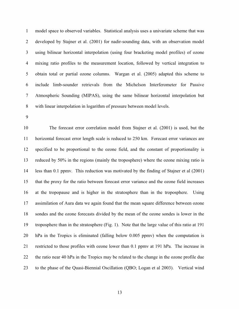
assimilation of Aura data we again found that the mean square difference between ozone
sondes and the ozone forecasts divided by the mean of the ozone sondes is lower in the
troposphere than in the stratosphere (Fig. 1). Note that the large value of this ratio at 191
hPa in the Tropics is eliminated (falling below 0.005 ppmv) when the computation is
restricted to those profiles with ozone lower than 0.1 ppmv at 191 hPa. The increase in
the ratio near 40 hPa in the Tropics may be related to the change in the ozone profile due
to the phase of the Quasi-Biennial Oscillation (QBO; Logan et al 2003). Vertical wind
13
1
2
3
4
shear due to the QBO is not reproduced well in GEOS-4 operational runs that are used
here, which do not employ a highly anisotropic, non-separable forecast error correlation
model developed by Gaspari et al. (2006).
5
6
7
8
9
10
11
12
Figure 1. The ratio of the mean square difference between ozone sonde observations and
forecasts from Aura assimilation divided by the mean of the sondes is shown for
the Tropics (solid), northern middle latitudes (dotted) and northern high latitude
(dashed) for year 2005.
14
1
2
3
4
5
6
7
8
9
10
11
12
13
14
15
16
17
18
19
20
21
22
23
Observation errors are modeled as uncorrelated. MLS retrieval precision, which
varies from about 2% to 15% in the middle stratosphere, but increases to ~50% in the
Tropics at 215 hPa, was used as the standard deviation of the observation errors in the
assimilation. OMI data were averaged onto 2° 2.5° grid prior to assimilation in order to
reduce the data volume and potentially improve data precision. As only cloud-free OMI
data are used, the number of OMI data per grid box has a nonuniform distribution with
the mode of 2 and mean of 33 observations per grid box. These averaged OMI data were
assimilated with the error standard deviation specified as 2%.
Three experiments are presented in comparisons. The main Aura assimilation
experiment that is evaluated here uses the statistics defined in this section. Two
additional experiments are: a perturbation experiment in which MLS observation errors
are reduced by 50% (in Section 6 only), and a model run (described in Section 3.1) that
does not assimilate any Aura data.
4. Ozone in the upper troposphere and lower stratosphere
This section discusses the representation of ozone structures in the UTLS of the
analyses. This is important, because ozone mixing ratios increase rapidly from
tropospheric values (<0.1 ppmv) to stratospheric values (often larger than 1 ppmv) over a
thin layer. Spatial variations in tropopause height lead to similar structure in horizontal
distributions of ozone. Accurate representation of these gradients and their location
relative to the tropopause is thus an important factor in computing the TOC. Further,
estimates of stratosphere-troposphere exchange (STE) of ozone depend on accurate
15
1
2
3
4
5
6
7
8
9
10
11
12
13
14
15
16
17
18
19
20
21
22
23
representation of the spatial gradients. Errors in model vertical transport, such as
excessive downwelling, become evident as biased ozone in the UTLS. Examples of
validation of the assimilated Aura ozone in the UTLS against independent sonde and
aircraft data are presented.
Stajner et al. (2001) showed that assimilation of SBUV and TOMS ozone did not
accurately constrain the profile shape in the UTLS, with a pronounced (~30%)
overestimation of ozone concentrations near 150 hPa. This was due to the lack of
constraint on ozone profiles in this region and a poor representation of transport in that
analysis. Assimilation of ozone from the limb-sounding MIPAS instrument reduced
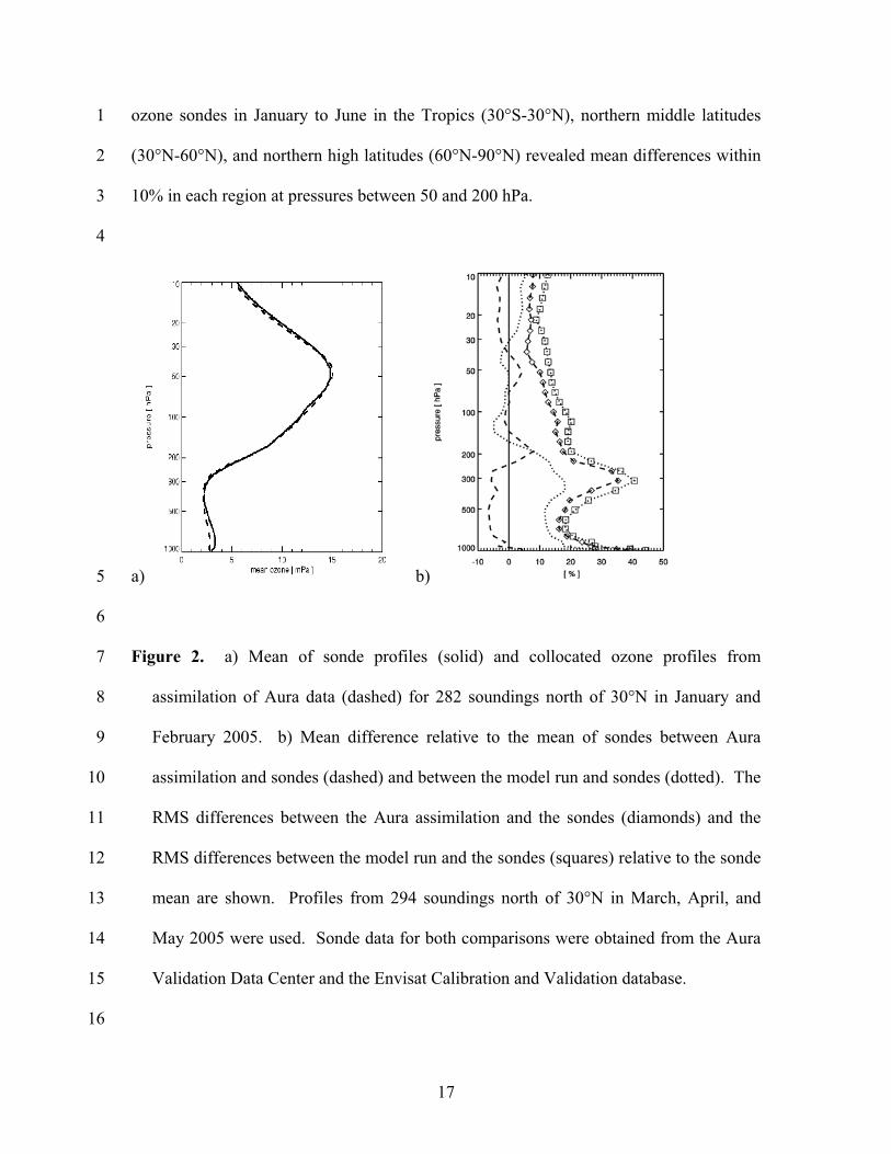
systematic errors in the lower stratosphere (Wargan et al. 2005). Figure 2a shows that the
systematic errors of the assimilated Aura ozone are small compared to independent ozone
sonde data in northern middle and high latitudes (30°N-90°N). Mean differences between
sonde measurements and collocated ozone profiles in January and February 2005 are less
than ±10% between 10 and 500 hPa. This improvement over Stajner et al. (2001) is due
to improved transport in this system (Pawson et al 2007) and to the assimilation of Aura
data. The latter is evident from the comparison of the model simulation using the same
meteorological fields (without the assimilation of Aura data) with the ozone sondes, and
Aura assimilated ozone in the same region during March, April, and May 2005 (Fig. 2b).
Ozone in the UTLS is overestimated in the model fields (by 19% near 300 hPa), in
comparison to the ozone sondes. In contrast, assimilation of the Aura data brings the
mean ozone to within 8% of the mean sonde profiles between the surface and 10 hPa.
Further comparisons focusing on the lower stratosphere (not shown) with all available
16
1
2
3
4
ozone sondes in January to June in the Tropics (30°S-30°N), northern middle latitudes
(30°N-60°N), and northern high latitudes (60°N-90°N) revealed mean differences within
10% in each region at pressures between 50 and 200 hPa.
a) b)5
6
7
8
9
10
11
12
13
14
15
16
Figure 2. a) Mean of sonde profiles (solid) and collocated ozone profiles from
assimilation of Aura data (dashed) for 282 soundings north of 30°N in January and
February 2005. b) Mean difference relative to the mean of sondes between Aura
assimilation and sondes (dashed) and between the model run and sondes (dotted). The
RMS differences between the Aura assimilation and the sondes (diamonds) and the
RMS differences between the model run and the sondes (squares) relative to the sonde
mean are shown. Profiles from 294 soundings north of 30°N in March, April, and
May 2005 were used. Sonde data for both comparisons were obtained from the Aura
Validation Data Center and the Envisat Calibration and Validation database.
17
1
2
3
4
5
6
7
8
9
10
11
12
13
14
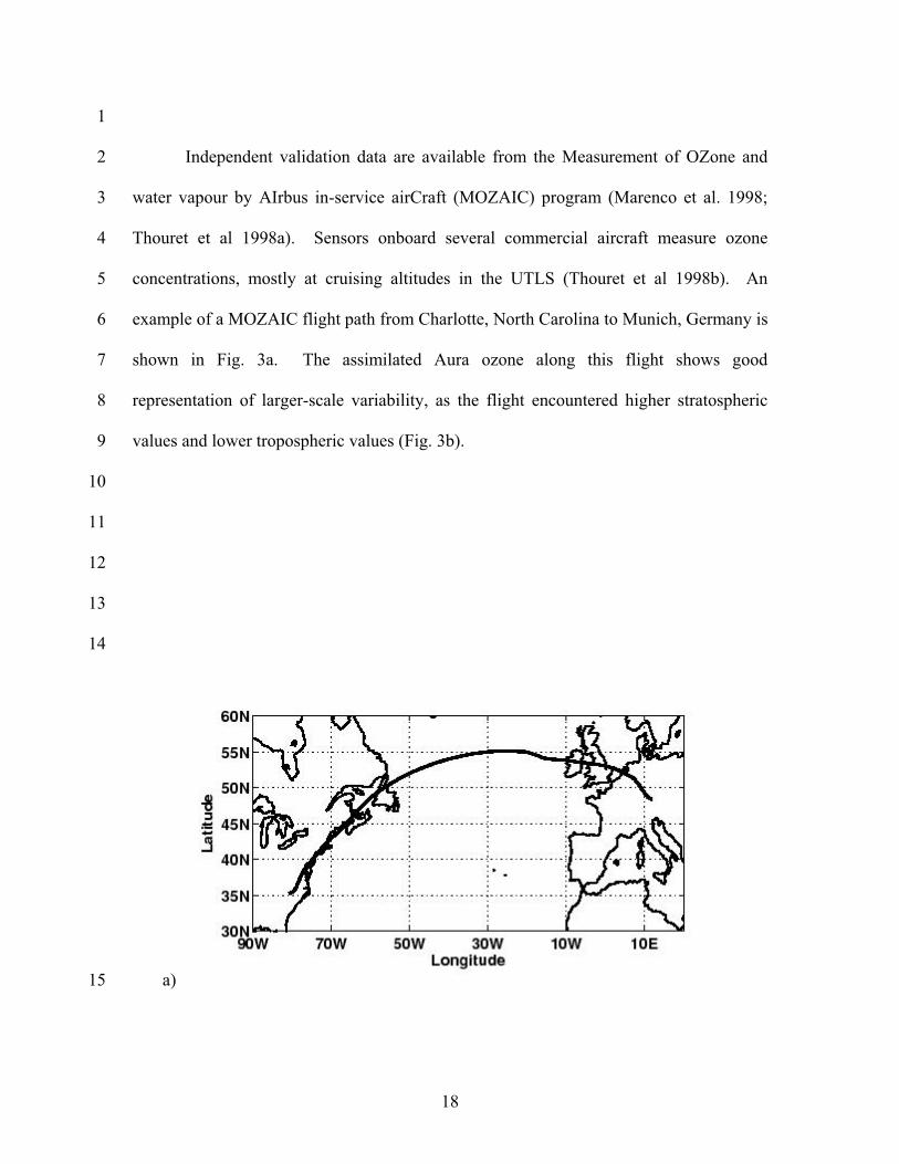
Independent validation data are available from the Measurement of OZone and
water vapour by AIrbus in-service airCraft (MOZAIC) program (Marenco et al. 1998;
Thouret et al 1998a). Sensors onboard several commercial aircraft measure ozone
concentrations, mostly at cruising altitudes in the UTLS (Thouret et al 1998b). An
example of a MOZAIC flight path from Charlotte, North Carolina to Munich, Germany is
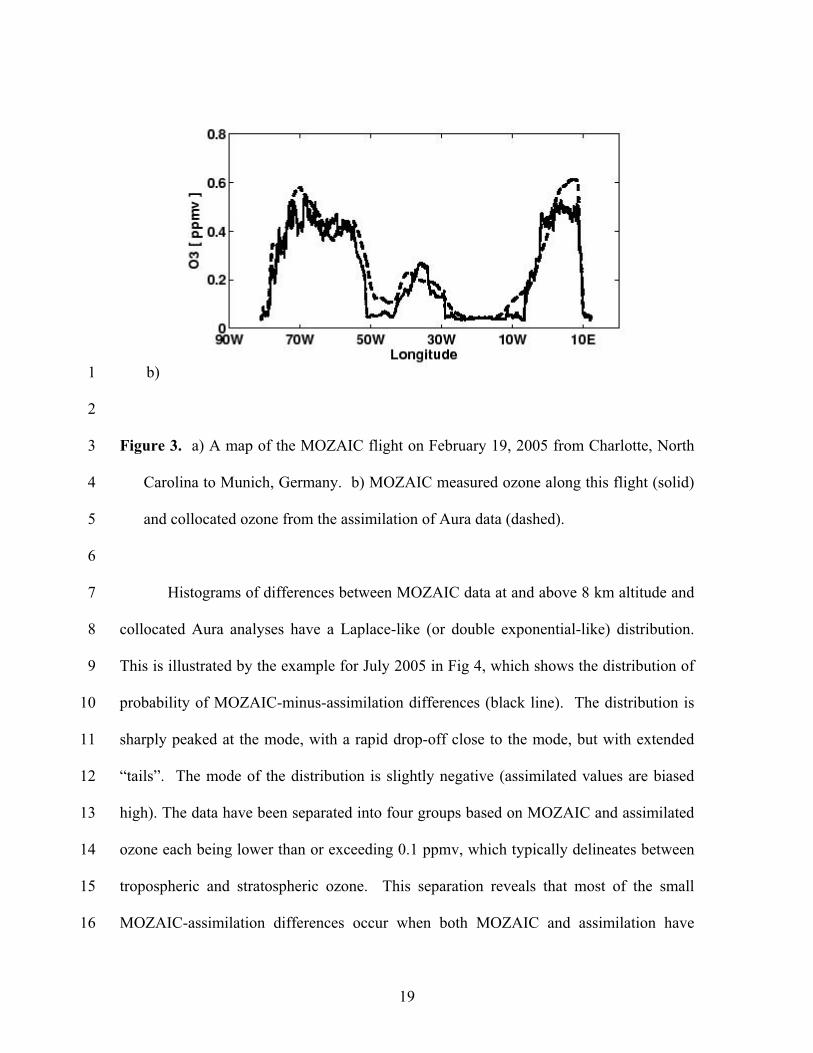
shown in Fig. 3a. The assimilated Aura ozone along this flight shows good
representation of larger-scale variability, as the flight encountered higher stratospheric
values and lower tropospheric values (Fig. 3b).
a)15
18
b)1
2
3
4
5
6
7
8
9
10
11
12
13
14
15
16
Figure 3. a) A map of the MOZAIC flight on February 19, 2005 from Charlotte, North
Carolina to Munich, Germany. b) MOZAIC measured ozone along this flight (solid)
and collocated ozone from the assimilation of Aura data (dashed).
Histograms of differences between MOZAIC data at and above 8 km altitude and
collocated Aura analyses have a Laplace-like (or double exponential-like) distribution.
This is illustrated by the example for July 2005 in Fig 4, which shows the distribution of
probability of MOZAIC-minus-assimilation differences (black line). The distribution is
sharply peaked at the mode, with a rapid drop-off close to the mode, but with extended
“tails”. The mode of the distribution is slightly negative (assimilated values are biased
high). The data have been separated into four groups based on MOZAIC and assimilated
ozone each being lower than or exceeding 0.1 ppmv, which typically delineates between
tropospheric and stratospheric ozone. This separation reveals that most of the small
MOZAIC-assimilation differences occur when both MOZAIC and assimilation have
19
1
2
3
4
5
6
7
8
9
10
11
12
13
14
15
16
17
18
19
20
21
22
23
tropospheric ozone values (<0.1 ppmv; green line). The largest contribution to the “tails”
of the distribution comes from the measurements for which MOZAIC and assimilation
both have stratospheric ozone values ( 0.1 ppmv; yellow line). Note also that the peak
stratospheric ozone differences occur close to the zero line, indicating that the MLS data
lead to a very high-quality global assimilation. The mode of the tropospheric differences
is slightly negative, leading to the negative offset in the total histogram, indicating that
tropospheric ozone values near the tropopause in the assimilation are biased high
compared to the MOZAIC data.
Laplace-like distributions were seen in the analysis of ozone data along flight
tracks of research aircraft in comparisons of measurements offset by a fixed distance
(Sparling and Bacmeister 2001). They found this type of distribution for all but very
short distances (which are more impacted by correlated instrument noise). We found that
the distribution of MOZAIC-minus-assimilated differences is comparable to along-track
differences of MOZAIC measurements offset by ~400 km. This is close to the distance
between four model grid points along the latitude circle in middle latitudes, which is
arguably the finest scale that is represented in the grid-point model. For example, about 6
grid points are needed to represent the discontinuity on one side of a square wave using
flux-form semi-Lagrangian piecewise parabolic method (see Fig. 4 in Lin and Rood
1996).
Mean differences between analyses and MOZAIC data at and above 8 km altitude
were evaluated for each month from January to August 2005 (not shown). They range
20
1
2
3
4
5
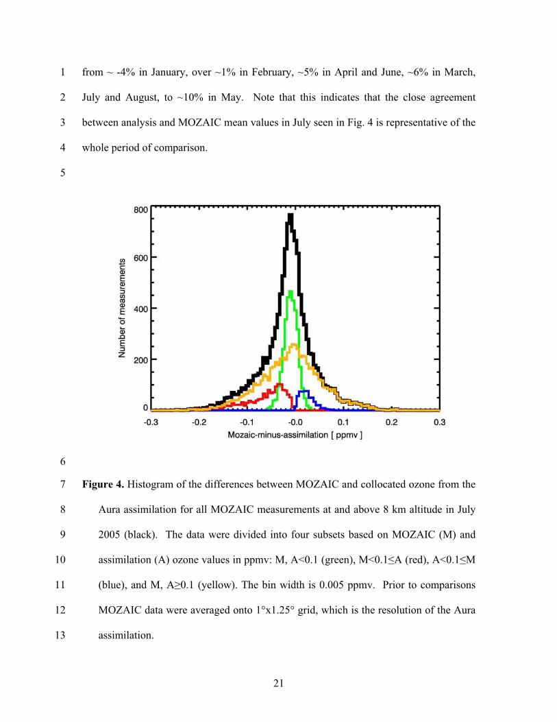
from ~ -4% in January, over ~1% in February, ~5% in April and June, ~6% in March,
July and August, to ~10% in May. Note that this indicates that the close agreement
between analysis and MOZAIC mean values in July seen in Fig. 4 is representative of the
whole period of comparison.
6
7
8
9
10
11
12
13
Figure 4. Histogram of the differences between MOZAIC and collocated ozone from the
Aura assimilation for all MOZAIC measurements at and above 8 km altitude in July
2005 (black). The data were divided into four subsets based on MOZAIC (M) and
assimilation (A) ozone values in ppmv: M, A<0.1 (green), M<0.1 A (red), A<0.1 M
(blue), and M, A 0.1 (yellow). The bin width is 0.005 ppmv. Prior to comparisons
MOZAIC data were averaged onto 1°x1.25° grid, which is the resolution of the Aura
assimilation.
21
1
2
3
4
5
6
7
8
9
10
11
12
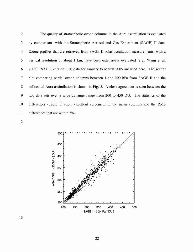
The quality of stratospheric ozone columns in the Aura assimilation is evaluated
by comparisons with the Stratospheric Aerosol and Gas Experiment (SAGE) II data.
Ozone profiles that are retrieved from SAGE II solar occultation measurements, with a
vertical resolution of about 1 km, have been extensively evaluated (e.g., Wang et al.
2002). SAGE Version 6.20 data for January to March 2005 are used here. The scatter
plot comparing partial ozone columns between 1 and 200 hPa from SAGE II and the
collocated Aura assimilation is shown in Fig. 5. A close agreement is seen between the
two data sets over a wide dynamic range from 200 to 450 DU. The statistics of the
differences (Table 1) show excellent agreement in the mean columns and the RMS
differences that are within 5%.
13
22
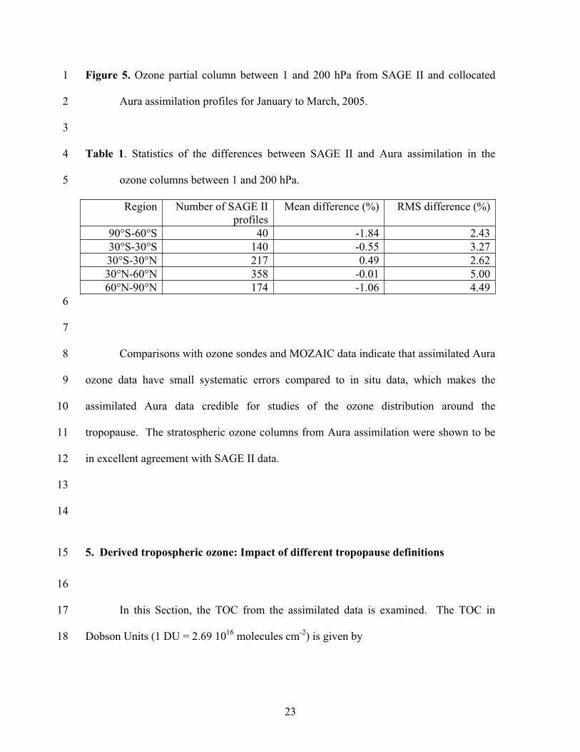
Figure 5. Ozone partial column between 1 and 200 hPa from SAGE II and collocated
Aura assimilation profiles for January to March, 2005.
1
2
3
4
5
Table 1. Statistics of the differences between SAGE II and Aura assimilation in the
ozone columns between 1 and 200 hPa.
Region Number of SAGE II
profiles
Mean difference (%) RMS difference (%)
90°S-60°S 40 -1.84 2.43
30°S-30°S 140 -0.55 3.27
30°S-30°N 217 0.49 2.62
30°N-60°N 358 -0.01 5.00
60°N-90°N 174 -1.06 4.49
6
7
8
9
10
11
12
13
14
15
16
17
18
Comparisons with ozone sondes and MOZAIC data indicate that assimilated Aura
ozone data have small systematic errors compared to in situ data, which makes the
assimilated Aura data credible for studies of the ozone distribution around the
tropopause. The stratospheric ozone columns from Aura assimilation were shown to be
in excellent agreement with SAGE II data.
5. Derived tropospheric ozone: Impact of different tropopause definitions
In this Section, the TOC from the assimilated data is examined. The TOC in
Dobson Units (1 DU = 2.69 1016
molecules cm-2
) is given by
23
ps
ptdp7891.0 ,1
2
3
4
5
6
7
8
9
10
11
12
13
14
15
16
17
18
19
20
21
22
23
where is the ozone mixing ratio in ppmv, p is pressure, pt is pressure of the chosen
tropopause, ps is the surface pressure (all pressures are in hPa). As discussed in Section
1, the information from observations that contributes to this product is limited to the
stratospheric and upper tropospheric profile (from MLS) and the total ozone column
(from OMI). Apart from the quality of the stratospheric ozone analyses and the total
column information, two other factors impact the determination of TOC. These are the
definition of the tropopause and the accuracy with which it can be located.
Ziemke et al. (2006) used the tropopause height determined from the lapse rate in
NCEP-NCAR reanalyses (Kistler et al. 2001). Birner et al. (2006) found that the
extratropical tropopause is too low and too warm in these analyses, consistent with results
of Schoeberl (2004) from other analyses. This uncertainty will result in an
underestimation of TOC. This aspect is not considered in this study, but remains an
important caveat in the estimations of TOC.
Early comparisons of several TOC products derived from EOS Aura data
suggested that some of the differences might be due to the choice of tropopause (G.
Morris, personal communication 2006). Schoeberl et al. (2007) avoid this issue by
comparing ozone columns between the surface and 200 hPa. This approach removes the
sensitivity to choice of tropopause, but it does not separate the tropospheric from the
stratospheric ozone.
24
1
2
3
4
5
6
7
8
9
10
11
12
13
14
15
16
17
18
19
20
21
22
There are valid reasons for using any of at least three different tropopause
definitions (e.g., Holton et al. 1995). In the WMO “thermal” definition, the tropopause is
the lower boundary of a layer in which temperature lapse rate is less than 2 K km-1
for a
depth of at least 2 km. Even though this definition can be applied to a single temperature
profile from a sounding or a model, it is not uniquely defined when multiple stable layers
are present (especially in the vicinity of the subtropical jet). The “dynamical” definition
of the tropopause relies on the increase in the potential vorticity (PV) from low values in
the troposphere to higher values in the stratosphere. This definition offers an advantage
over the thermal definition in that it is determined by the three-dimensional motion of air,
which provides a more faithful representation of the tropopause evolution during the
passage of wave disturbances. Even with this definition, various PV isopleths (ranging
between 1 and 4 PVU) have been applied to define the tropopause from three-
dimensional meteorological fields (e.g. Hoerling et al 1991). A third way of defining the
tropopause results from changes in the chemical composition of air at the tropopause. For
example, stratospheric air is rich in ozone, but has less carbon monoxide and water vapor
than the tropospheric air. A “chemical” definition of the tropopause relies on values of a
constituent, or its vertical gradient, exceeding a specified threshold (Bethan et al. 1996).
High resolution measurements of constituents near the tropopause support the notion of a
tropopause layer in which the transition of the chemical composition occurs over a couple
of kilometers or more, rather than at a single tropopause surface (Pan et al. 2004; Zahn et
al. 2000).
25
1
2
3
4
5
6
7
8
9
10
11
12
13
14
15
16
17
18
19
20
21
22
23
Here, the assimilated global ozone distributions are used to investigate sensitivity
of TOC to the definition of the tropopause. This exploits the availability of time-
dependent, three-dimensional ozone concentrations in the analyses in a way that is not
possible with more traditional TOC estimation methods (e.g., Ziemke et al., 2006). Four
tropopause definitions (Table 2) will be used in this sensitivity study. GEOS-4
meteorological fields are used to determine the WMO and dynamical tropopauses.
Assimilated Aura ozone data are used to determine ozone tropopause (searching for 0.1
ppmv in the profiles from below, i.e. starting at 500 hPa and proceeding towards higher
altitude) and “ozone tropopause from above” where 0.1 ppmv is found by the search from
above, which begins near 51 hPa and proceeds downward towards the surface.
Comparisons of the tropopauses according to WMO and dynamical definitions have been
made in global models and assimilated fields (e.g. Hoerling et al 1991). Comparisons of
tropopause defined according to WMO and ozone definitions are possible from in situ
measurements from ozone sondes and research or commercial aircraft (Bethan et al.
1996; Pan et al. 2004; Zahn et al. 2000). Such comparisons can be made for the global
ozone distribution in the assimilated data. Differences in the position of the tropopause
according to these definitions may provide an indication of the thickness of the
tropopause layer over which air characteristics change from tropospheric to stratospheric.
Table2. The four tropopause definitions used are listed (column 1). The criterion used
for each definition is given (column 2), together with the pressure range over
26
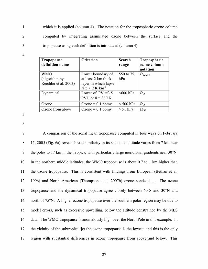
1
2
3
4
which it is applied (column 4). The notation for the tropospheric ozone column
computed by integrating assimilated ozone between the surface and the
tropopause using each definition is introduced (column 4).
Tropopause
definition name
Criterion Search
range
Tropospheric
ozone column
notation
WMO
(algorithm by
Reichler et al. 2003)
Lower boundary of
at least 2 km thick
layer in which lapse
rate < 2 K km-1
550 to 75
hPaWMO
Dynamical Lower of |PV| =3.5
PVU or = 380 K
<600 hPa D
Ozone Ozone = 0.1 ppmv < 500 hPa O
Ozone from above Ozone = 0.1 ppmv > 51 hPa OA
5
6
7
8
9
10
11
12
13
14
15
16
17
18
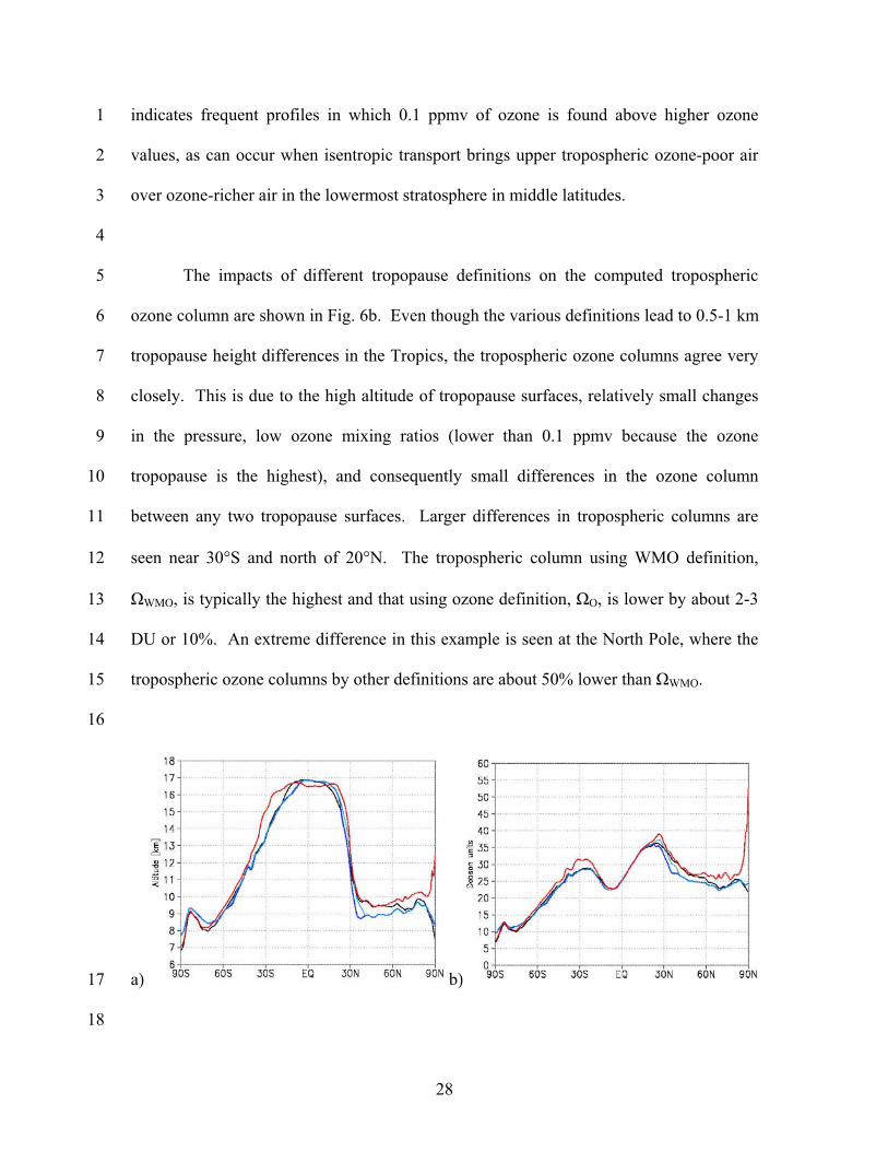
A comparison of the zonal mean tropopause computed in four ways on February
15, 2005 (Fig. 6a) reveals broad similarity in its shape: its altitude varies from 7 km near
the poles to 17 km in the Tropics, with particularly large meridional gradients near 30 N.
In the northern middle latitudes, the WMO tropopause is about 0.7 to 1 km higher than
the ozone tropopause. This is consistent with findings from European (Bethan et al.
1996) and North American (Thompson et al 2007b) ozone sonde data. The ozone
tropopause and the dynamical tropopause agree closely between 60 S and 30 N and
north of 75 N. A higher ozone tropopause over the southern polar region may be due to
model errors, such as excessive upwelling, below the altitude constrained by the MLS
data. The WMO tropopause is anomalously high over the North Pole in this example. In
the vicinity of the subtropical jet the ozone tropopause is the lowest, and this is the only
region with substantial differences in ozone tropopause from above and below. This
27
1
2
3
4
5
6
7
8
9
10
11
12
13
14
15
16
indicates frequent profiles in which 0.1 ppmv of ozone is found above higher ozone
values, as can occur when isentropic transport brings upper tropospheric ozone-poor air
over ozone-richer air in the lowermost stratosphere in middle latitudes.
The impacts of different tropopause definitions on the computed tropospheric
ozone column are shown in Fig. 6b. Even though the various definitions lead to 0.5-1 km
tropopause height differences in the Tropics, the tropospheric ozone columns agree very
closely. This is due to the high altitude of tropopause surfaces, relatively small changes
in the pressure, low ozone mixing ratios (lower than 0.1 ppmv because the ozone
tropopause is the highest), and consequently small differences in the ozone column
between any two tropopause surfaces. Larger differences in tropospheric columns are
seen near 30 S and north of 20 N. The tropospheric column using WMO definition,
WMO, is typically the highest and that using ozone definition, O, is lower by about 2-3
DU or 10%. An extreme difference in this example is seen at the North Pole, where the
tropospheric ozone columns by other definitions are about 50% lower than WMO.
a) b)17
18
28
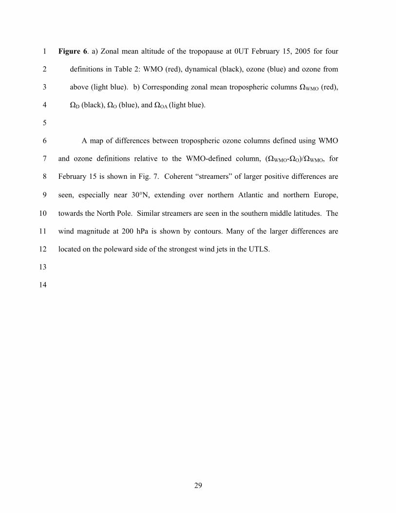
Figure 6. a) Zonal mean altitude of the tropopause at 0UT February 15, 2005 for four
definitions in Table 2: WMO (red), dynamical (black), ozone (blue) and ozone from
above (light blue). b) Corresponding zonal mean tropospheric columns WMO (red),
D (black), O (blue), and OA (light blue).
1
2
3
4
5
6
7
8
9
10
11
12
13
14
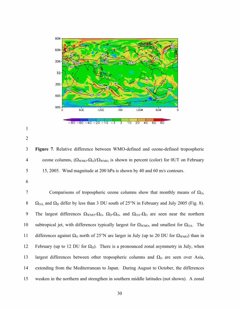
A map of differences between tropospheric ozone columns defined using WMO
and ozone definitions relative to the WMO-defined column, ( WMO- O)/ WMO, for
February 15 is shown in Fig. 7. Coherent “streamers” of larger positive differences are
seen, especially near 30 N, extending over northern Atlantic and northern Europe,
towards the North Pole. Similar streamers are seen in the southern middle latitudes. The
wind magnitude at 200 hPa is shown by contours. Many of the larger differences are
located on the poleward side of the strongest wind jets in the UTLS.
29
1
2
3
4
5
6
7
8
9
10
11
12
13
14
15
Figure 7. Relative difference between WMO-defined and ozone-defined tropospheric
ozone columns, ( WMO- O)/ WMO, is shown in percent (color) for 0UT on February
15, 2005. Wind magnitude at 200 hPa is shown by 40 and 60 m/s contours.
Comparisons of tropospheric ozone columns show that monthly means of O,
OA, and D differ by less than 3 DU south of 25°N in February and July 2005 (Fig. 8).
The largest differences WMO- O, D- O, and OA- O are seen near the northern
subtropical jet, with differences typically largest for WMO, and smallest for OA. The
differences against O north of 25°N are larger in July (up to 20 DU for WMO) than in
February (up to 12 DU for D). There is a pronounced zonal asymmetry in July, when
largest differences between other tropospheric columns and O are seen over Asia,
extending from the Mediterranean to Japan. During August to October, the differences
weaken in the northern and strengthen in southern middle latitudes (not shown). A zonal
30
1
2
3
4
5
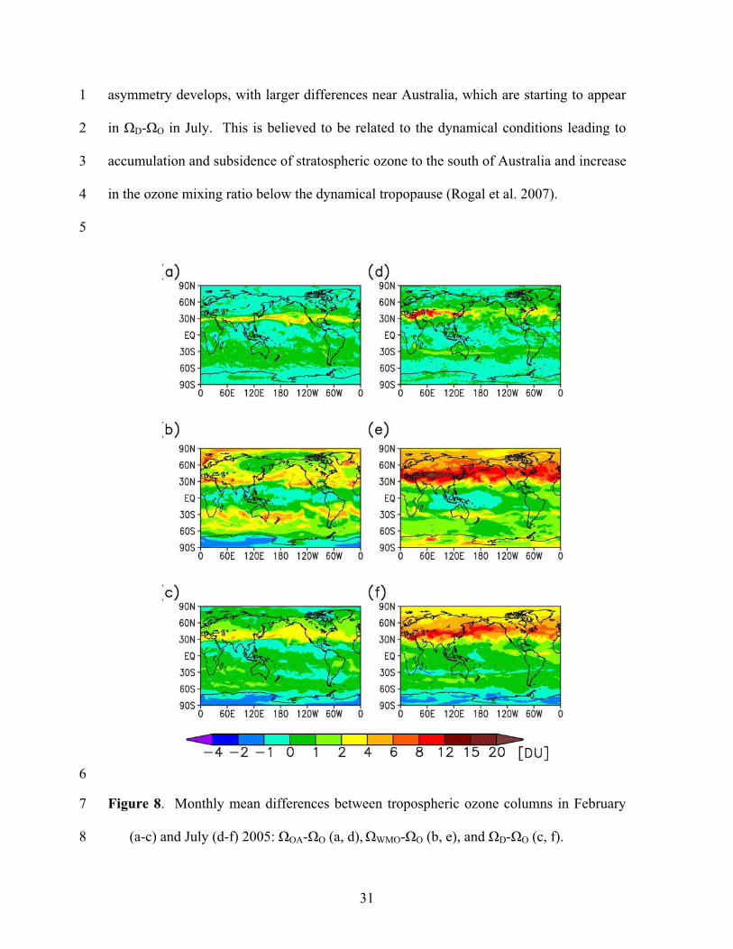
asymmetry develops, with larger differences near Australia, which are starting to appear
in D- O in July. This is believed to be related to the dynamical conditions leading to
accumulation and subsidence of stratospheric ozone to the south of Australia and increase
in the ozone mixing ratio below the dynamical tropopause (Rogal et al. 2007).
6
7
8
Figure 8. Monthly mean differences between tropospheric ozone columns in February
(a-c) and July (d-f) 2005: OA- O (a, d), WMO- O (b, e), and D- O (c, f).
31
1
2
3
4
5
6
7
8
9
10
11
12
13
14
15
16
17
18
19
Focusing on a small European region (50 N-80 N, 0 E-20 E) during fall and
winter months in 2005, we examine the distribution of ( WMO- O)/ WMO. This is chosen
to allow comparison with the results of Bethan et al. (1996) who used sonde
measurements within this region, mostly in fall and winter months. The distribution from
Aura assimilation (Fig. 9) resembles their findings from sondes (op. cit.). Even though
O is often higher than WMO by less than 5%, for the vast majority of cases, O is lower
than WMO, occasionally by more than 80%. In the Aura assimilation for 2005 the latter
cases occur in February, when strong winds are seen in the UTLS region in the Northern
Atlantic, approaching Northern Europe. This is consistent with findings of Bethan et al.
(1996) that the largest differences between WMO and O are found on the cyclonic side
of strong jets in profiles with “indefinite thermal tropopause”. They use this term for
profiles in which lapse rate changes slowly from typical tropospheric to stratospheric
values over several km thick layers. Large differences are not confined to winter: an
example of ozone sonde profile with the WMO tropopause higher than the ozone
tropopause by 6.9 km and O lower than WMO, by 56% was presented by Thompson et
al (2007b).
32
1
2
3
4
5
6
7
8
9
10
11
12
13
14
15
16
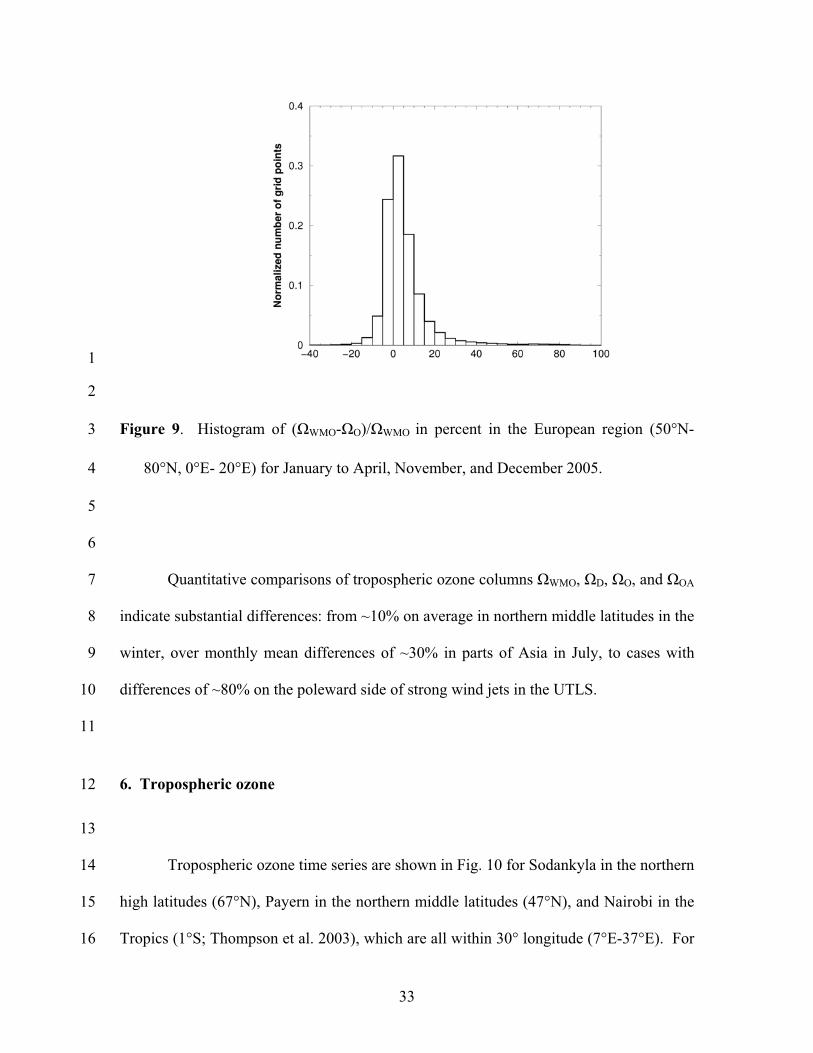
Figure 9. Histogram of ( WMO- O)/ WMO in percent in the European region (50 N-
80 N, 0 E- 20 E) for January to April, November, and December 2005.
Quantitative comparisons of tropospheric ozone columns WMO, D, O, and OA
indicate substantial differences: from ~10% on average in northern middle latitudes in the
winter, over monthly mean differences of ~30% in parts of Asia in July, to cases with
differences of ~80% on the poleward side of strong wind jets in the UTLS.
6. Tropospheric ozone
Tropospheric ozone time series are shown in Fig. 10 for Sodankyla in the northern
high latitudes (67°N), Payern in the northern middle latitudes (47°N), and Nairobi in the
Tropics (1°S; Thompson et al. 2003), which are all within 30° longitude (7°E-37°E). For
33
1
2
3
4
5
6
7
8
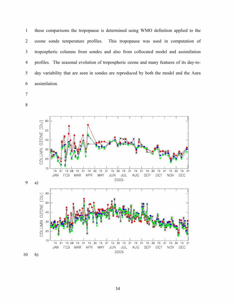
these comparisons the tropopause is determined using WMO definition applied to the
ozone sonde temperature profiles. This tropopause was used in computation of
tropospheric columns from sondes and also from collocated model and assimilation
profiles. The seasonal evolution of tropospheric ozone and many features of its day-to-
day variability that are seen in sondes are reproduced by both the model and the Aura
assimilation.
a)9
b)10
34
c)1
2
3
4
5
6
7
8
9
10
11
12
13
14
15
16
17
18
19
20
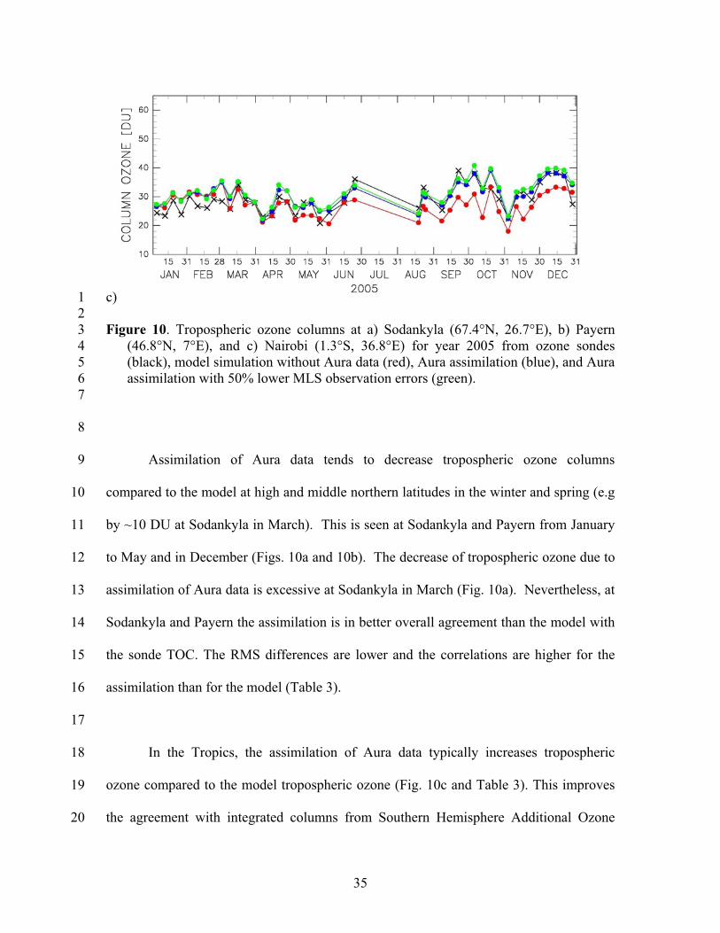
Figure 10. Tropospheric ozone columns at a) Sodankyla (67.4°N, 26.7°E), b) Payern
(46.8°N, 7°E), and c) Nairobi (1.3°S, 36.8°E) for year 2005 from ozone sondes
(black), model simulation without Aura data (red), Aura assimilation (blue), and Aura
assimilation with 50% lower MLS observation errors (green).
Assimilation of Aura data tends to decrease tropospheric ozone columns
compared to the model at high and middle northern latitudes in the winter and spring (e.g
by ~10 DU at Sodankyla in March). This is seen at Sodankyla and Payern from January
to May and in December (Figs. 10a and 10b). The decrease of tropospheric ozone due to
assimilation of Aura data is excessive at Sodankyla in March (Fig. 10a). Nevertheless, at
Sodankyla and Payern the assimilation is in better overall agreement than the model with
the sonde TOC. The RMS differences are lower and the correlations are higher for the
assimilation than for the model (Table 3).
In the Tropics, the assimilation of Aura data typically increases tropospheric
ozone compared to the model tropospheric ozone (Fig. 10c and Table 3). This improves
the agreement with integrated columns from Southern Hemisphere Additional Ozone
35
36
1
2
3
4
5
6
7
8
9
10
11
12
13
14
15
16
17
18
19
sondes (SHADOZ; Thompson et al. 2003) over South America, the Atlantic, Africa, and
the Indian Ocean (Table 3), but also leads to an overestimate of tropospheric ozone over
the Pacific (Table 3). For example, at Pago Pago (14.2°S, 189.4°E;) tropospheric ozone
from Aura assimilation is higher by 5.52 DU on average than that from the sonde profiles
during year 2005. Assimilated tropospheric column at Pago Pago is also higher than
model tropospheric column. This is consistent with findings of Ziemke et al (2006) in the
tropical Pacific, where tropospheric column residual determined from OMI and MLS data
is larger than that simulated by a CTM.
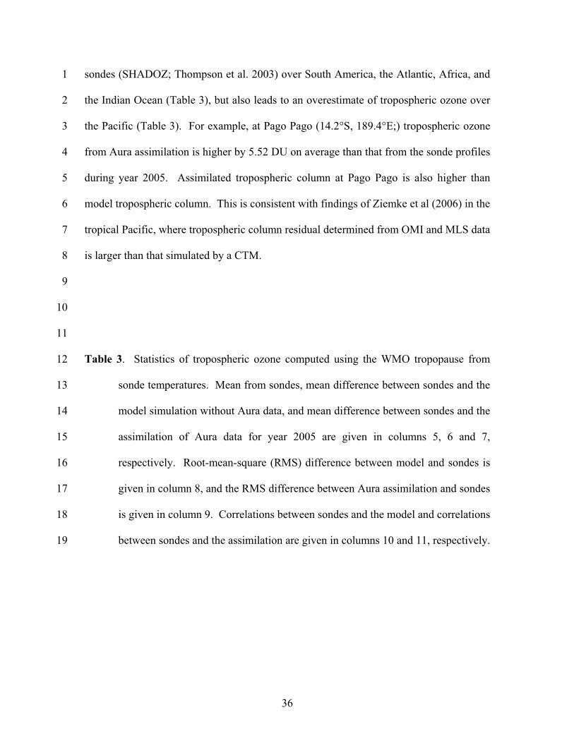
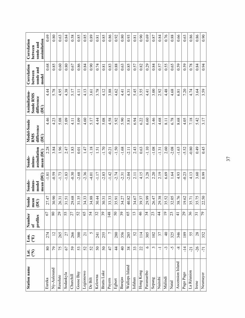
Table 3. Statistics of tropospheric ozone computed using the WMO tropopause from
sonde temperatures. Mean from sondes, mean difference between sondes and the
model simulation without Aura data, and mean difference between sondes and the
assimilation of Aura data for year 2005 are given in columns 5, 6 and 7,
respectively. Root-mean-square (RMS) difference between model and sondes is
given in column 8, and the RMS difference between Aura assimilation and sondes
is given in column 9. Correlations between sondes and the model and correlations
between sondes and the assimilation are given in columns 10 and 11, respectively.
Sta
tion
nam
e L
at.
(°N
)
Lo
n.
(°E
)
Nu
mb
er
of
pro
file
s
So
nd
e
mea
n
(DU
)
So
nd
e-
min
us-
mod
el
mea
n (
DU
)
So
nd
e-
min
us-
ass
imil
ati
on
mea
n (
DU
)
Mod
el-S
on
de
RM
S
dif
fere
nce
(DU
)
Ass
imil
ati
on
-
So
nd
e R
MS
dif
fere
nce
(DU
)
Co
rrel
ati
on
bet
wee
n
son
de
an
d
mod
el
Co
rrel
ati
on
bet
wee
n
son
de
an
d
ass
imil
ati
on
Eu
rek
a 8
02
74
6
72
7.4
7
-1.8
1
2.2
8
4.4
6
4.4
4
0.6
8
0.6
9
Ny
-Aal
esu
nd
7
91
28
03
0.9
0
-0.5
9
3.8
4
4.2
3
5.7
8
0.8
5
0.8
0
Res
olu
te
75
265
2
92
6.3
1
-1.7
3
1.9
6
5.0
8
4.9
5
0.6
0
0.6
3
Sodan
kyla
67
2
7
55
31.5
1
-1.8
3
2.4
7
5.0
9
4.3
8
0.8
0
0.8
4
Churc
hil
l 5
92
66
2
72
9.6
8
-0.3
0
1.8
3
4.1
1
5.1
7
0.6
7
0.5
8
Goose
Bay
5
33
00
5
23
1.3
5
-2.6
8
0.0
1
5.0
9
4.1
1
0.8
6
0.8
5
Leg
ionow
o
52
21
65
34.3
3
-2.3
6
1.4
7
4.6
0
4.1
3
0.8
4
0.8
5
De
Bil
t 5
25
54
34.8
8
-4.0
1
-1.1
8
5.1
7
3.6
1
0.9
0
0.8
9
Kel
ow
na
5
02
41
3
23
0.4
4
-1.1
7
1.5
1
4.4
4
3.7
8
0.7
4
0.8
1
Bra
tts
Lak
e 5
02
55
3
93
0.3
1
-2.8
3
-1.7
0
5.0
8
4.1
2
0.8
1
0.8
5
Pay
ern
4
7
7
1
48
3
3.3
3
-1.4
2
-0.2
1
4.5
8
3.8
8
0.8
3
0.8
6
Egber
t4
42
80
5
03
5.9
1
-2.7
4
-1.5
0
5.9
2
4.6
2
0.8
8
0.9
2
Bar
ajas
4
03
56
3
93
4.2
7
-2.3
1
-1.6
8
5.9
0
4.4
1
0.6
3
0.8
0
Wal
lops
Isla
nd
38
285
6
54
0.8
2
-2.0
4
-2.1
1
5.8
1
4.3
1
0.8
5
0.9
3
Isfa
han
3
35
21
33
4.6
7
2.1
1
2.4
3
6.9
4
5.4
5
0.5
7
0.8
1
Hong
Kong
2
21
14
4
63
9.3
7
4.1
5
0.6
3
6.2
2
3.5
5
0.8
2
0.9
0
Par
amar
ibo
6
305
3
42
9.9
9
3.2
8
-1.1
0
6.6
0
4.4
1
0.2
9
0.6
9
Sep
ang
3
1
02
2
32
6.4
7
2.2
0
-1.0
8
3.4
6
3.0
0
0.8
4
0.8
7
Nai
rob
i
-1
3
7
44
29.3
8
2.1
9
-1.3
1
4.6
8
2.9
2
0.5
7
0.8
4
Mal
ind
i
-3
40
1
93
5.5
2
6.6
9
2.6
0
8.1
1
4.4
8
0.5
5
0.7
6
Nat
al
-5
3
25
2
33
2.0
5
1.6
4
-2.0
8
6.7
8
4.6
8
0.6
5
0.8
8
Asc
ensi
on
Isl
and
-8
3
46
4
13
8.7
6
4.9
3
-1.6
3
8.6
8
6.8
1
0.5
9
0.6
6
Pag
o P
ago
-
14
189
2
91
9.6
2
-0.2
3
-5.5
2
4.0
5
7.2
0
0.5
9
0.6
3
La
Réu
nio
n
-2
1
5
5
36
35.7
1
4.1
3
-0.8
0
7.1
8
4.7
4
0.7
8
0.8
6
Iren
e -
26
28
3
13
5.7
5
3.6
0
0.4
9
5.4
2
3.6
4
0.8
4
0.8
6
Neu
may
er
-71
3
52
7
92
2.5
0
0.9
9
0.4
5
3.1
7
3.5
9
0.9
4
0.9
0
37
1
2
3
4
5
6
7
8
9
10
11
12
13
14
15
16
17
18
19
20
21
22
23
Observed-minus-forecast (O-F) residuals, i.e. differences between the incoming
data and model forecast of the same variables are routinely computed during the
assimilation cycle, and they can provide information about observation error
characteristics (e.g. Stajner et al 2004). Inspection of zonal means and maps of OMI total
ozone column O-F residuals reveals that they are consistent with the changes in the
tropospheric ozone columns seen in Fig. 10, i.e. OMI O-F residuals tend to be positive in
the Tropics, especially in the Pacific. OMI O-F residuals are often negative outside the
Tropics, e.g. in the northern hemisphere in March.
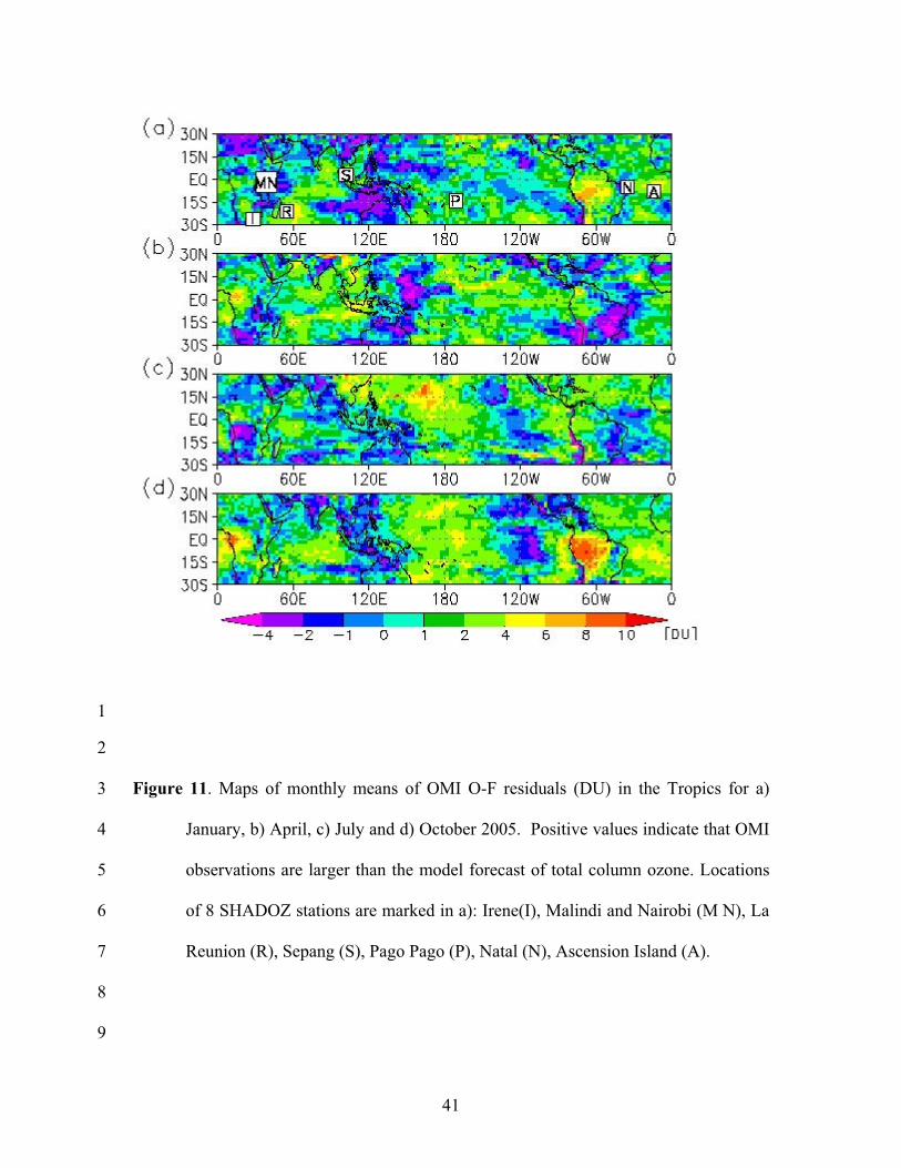
Examples of monthly-mean OMI O-F residuals in the Tropics are shown in Fig.
11. In January (Fig. 11a) the monthly mean of OMI O-Fs is within ±4 DU in most
regions, and it exceeds 4 DU in the Indian Ocean near La Reunion (21.1°S, 55.5°E), in
the South America, and near 5°S in the Atlantic. The character of OMI-model
discrepancies is somewhat different in each of these three regions. At La Reunion model
TOCs are lower than those from sondes in January, so positive OMI O-Fs lead to
increased TOCs in the assimilation and an improved agreement with sonde TOCs. In the
South America (from about 10°S, 280°E to about 5°S, 300°E) mean OMI O-Fs exceed 6
DU, however this is also a region with frequent clouds where reflectivity is often higher
than 15%, so OMI observations are assimilated for fewer than 15 days in January. Data
gaps during assimilation are known to often lead to accumulation of model errors and
consequently larger O-F residuals. In the Atlantic near 5°S positive OMI O-Fs yield
38
1
2
3
4
5
6
7
8
9
10
11
12
13
14
15
16
17
18
19
20
21
22
23
higher tropospheric ozone in the assimilation compared to both the model and the nearby
ozone sonde station on the Ascension Island (8°S, 345.6°E). The OMI O-Fs are slightly
lower in this region when MLS data are assimilated using lower error specifications
providing a tighter constraint on ozone in the lower stratosphere (not shown). Thus,
larger OMI O-F in the Atlantic may be an indication of errors in the transport and in the
representation of vertical ozone gradients in the lower stratosphere.
In April mean OMI O-Fs are negative over southern Africa, western Pacific,
Australia and parts of South America (Fig. 11b). In contrast, OMI O-Fs are positive over
the Indian Ocean, the central and eastern Pacific Ocean, and the region spanning the
southern Atlantic Ocean and equatorial Africa. In October OMI O-Fs over South
America and Africa exceed 6 DU indicating that ozone production may be stronger than
specified in the model. Note that tropospheric ozone columns in the assimilation respond
to the OMI O-F residuals. Inspection of monthly differences in tropospheric ozone
columns between Aura assimilation and model simulations indicates similar patterns to
those seen in OMI O-F residual maps in Fig. 11: tropospheric columns increase the most
in the Aura assimilation compared to the model simulation in the regions where OMI O-F
residuals are the largest. A persistent drought in the Amazon basin lead to increased
biomass burning in October 2005 (Zeng et al. 2007). The model uses climatological
biomass burning emissions, and thus underestimates ozone production in this region.
Assimilation of Aura OMI data increases the tropospheric ozone by about 10 DU in this
region and greatly improves the agreement with ozone sondes in Natal and Paramaribo
during September–December.
39
1
2
3
4
5
6
7
8
9
10
11
12
Positive OMI O-Fs are seen in monthly means from May to December 2005 in the
western and central Pacific (see e.g. July and October in Figs. 11c and 11d). The
assimilation of OMI data increases total ozone columns there, while MLS data are
constraining stratospheric profiles, leading to accumulation of ozone in the troposphere.
This is consistent with the overestimation of the TOC in the assimilation at Pago Pago
(Table 3), which was found in the comparison of Aura assimilation with ozone sondes
from March 25 to the end of the year. Even though this could implicate OMI data as the
source of differences between TOC from ozone sondes and the Aura assimilation, errors
in other components of the assimilation system (e.g. MLS data and transport of ozone in
the model) as well as the quality of ozone sonde data need to be considered.
40
1
2
3
4
5
6
7
8
9
Figure 11. Maps of monthly means of OMI O-F residuals (DU) in the Tropics for a)
January, b) April, c) July and d) October 2005. Positive values indicate that OMI
observations are larger than the model forecast of total column ozone. Locations
of 8 SHADOZ stations are marked in a): Irene(I), Malindi and Nairobi (M N), La
Reunion (R), Sepang (S), Pago Pago (P), Natal (N), Ascension Island (A).
41
1
2
3
4
5
6
7
8
9
10
11
12
13
14
15
16
17
18
19
20
21
22
23
The residual circulation is known to be overly strong in the GEOS-4 analyses
(Pawson et al. 2007), which leads to a deficit in stratospheric ozone in the Tropics and an
excess in the extra-tropics. The MLS O-F residuals between ~1 and 50 hPa, and the
analysis increments (i.e. changes in the ozone field due to the assimilation of
observational data) are consistent with this scenario. We note in passing that horizontal
mixing across the subtropical barrier does not seem to be excessive in GEOS-4.0.3 (cf.
Bloom et al. 2005), as it was in earlier versions of the transport (Tan et al. 2004). With
an earlier version of the transport (from GEOS-4.0.1), Wargan et al. (2005) found that
ozone analysis increments due to assimilation of data from MIPAS limb sounding
instrument were systematically counteracting the reduction of the ozone gradients, which
was caused by an excessive mixing across the subtropical barrier.
Version 1.5 of the MLS data is known to be biased high in the UTLS. The lowest
MLS level being assimilated is near 215 hPa. In the Tropics this level is usually in the
upper troposphere, and in the extratropics it is often in the lower stratosphere. Thus,
MLS data could contribute directly to higher tropical tropospheric ozone. By increasing
stratospheric ozone in the extratropics, for a fixed OMI total column, they could
indirectly cause lower tropospheric column residual. Note that even though MLS data
are assimilated at 215 hPa, the error specifications are large (e.g. ~20%-50% in the
Tropics), so that analyses are not strongly drawn to MLS data at that level. In order to
separate the impact of MLS data we assimilated Aura data in another experiment in
which MLS observation error standard deviations were specified as 50% lower. The
impact of this change is about 1 DU on the tropospheric column, decreasing it in the
42
1
2
3
4
5
6
7
8
9
10
11
12
13
14
15
16
17
18
19
20
21
22
23
northern high and middle latitudes in winter and spring. Impacts in the Tropics vary with
season and location: increases are mostly found close to the Equator, and decreases
towards subtropics. These changes are too small to explain the biases shown in Fig. 10.
Retrieved OMI total ozone columns incorporate prior information provided by an
ozone climatology, which varies with latitude and time, but is zonally symmetric
(McPeters et al 2007a). However, there is pronounced zonal variability in tropospheric
ozone in the Tropics with higher ozone in the Atlantic than in the Pacific basin (e.g.
Thompson et al 2003). This wave one feature in the tropospheric ozone may lead to
overestimation of ozone in the Pacific. Indeed, Thompson et al. (2007a) found that
Version 8 retrievals of total ozone columns from the Earth Probe TOMS instrument are
typically higher than the total ozone columns retrieved from the Dobson instrument and
from integration of sonde profiles at Pago Pago, with larger differences against the latter.
Note that Version 8 TOMS retrievals are very similar to the OMI total ozone retrievals
used here.
There are also known issues with the ozone sonde data at Pago Pago (Thompson
et al. 2007a). At this station Science Pump Model 6A sondes are used with a 2% KI
unbuffered solution. Even after a pump correction factor is applied to the sonde
measurements, reported ozone data are estimated to be about 9% to 10% lower than the
true values between the surface and 10 km altitude. These estimates were obtained by
simulating the flight conditions in a chamber and comparing with more accurate
measurements. In addition, total ozone obtained from sonde measurements is by 7%-8%
43
1
2
3
4
5
6
7
8
9
10
11
12
13
14
15
16
17
18
19
20
21
22
23
lower than that from a collocated Dobson spectrophotometer between the end of March
25 and December 31, 2005 (Samuel Oltmans, personal communication 2007). If a
uniform 10% correction were applied to the Pago Pago sonde data, the RMS difference
between TOCs from the sondes and from the model or assimilation experiments would be
as follows: 4.55 DU for the model, 5.89 DU for the Aura assimilation, and 5.59 DU for
the Aura assimilation with 50% reduced MLS error specifications. Thus, the RMS
differences would increase for the model (4.55 DU compared to 4.05 DU in Table 3), and
decrease for the Aura assimilation (5.89 DU compared to 7.20 DU in Table 3).
The TOCs from the Aura assimilation were found to reproduce the annual cycle
and some of the day-to-day variability in comparison with ozone sondes (Fig. 10). The
RMS differences in the TOCs against the ozone sonde data are reduced in the
assimilation of Aura data to about 2.9-7.4 DU compared to those from model simulation,
which range from 3.2 DU to 8.7 DU (Table 3). The correlation with sonde tropospheric
columns is also higher for the assimilation of Aura data (0.58-0.93) than for the model
run (0.29-0.93). OMI O-F residuals provide a quantitative measure of data-model
discrepancies, which are later reflected in the impacts of Aura data on the estimated
ozone columns. Using the Pacific example, it was illustrated that interplay between
different components of the assimilations system needs to be considered when evaluating
impacts of assimilation on the TOCs. Furthermore, in the evaluation of the quality of the
TOC estimates, the biases in the comparative data needs to be considered as well (e.g. for
Pago Pago ozone sondes).
44
1
2
3
4
5
6
7
8
9
10
11
12
13
14
15
16
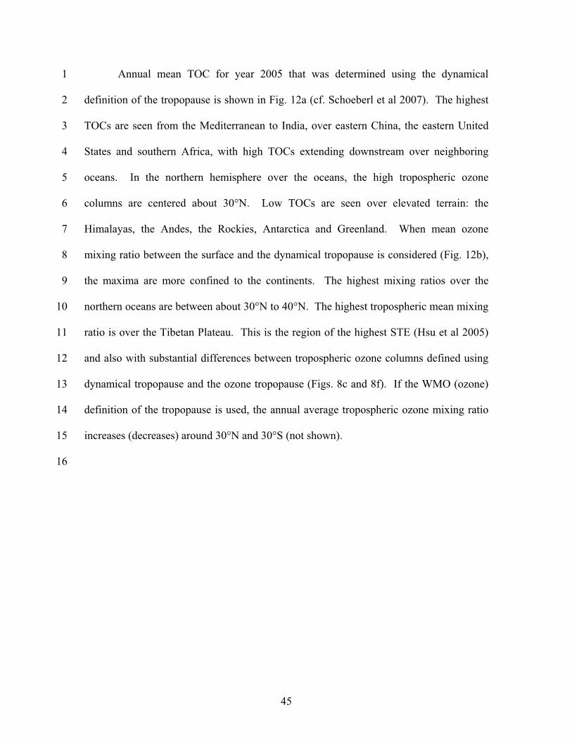
Annual mean TOC for year 2005 that was determined using the dynamical
definition of the tropopause is shown in Fig. 12a (cf. Schoeberl et al 2007). The highest
TOCs are seen from the Mediterranean to India, over eastern China, the eastern United
States and southern Africa, with high TOCs extending downstream over neighboring
oceans. In the northern hemisphere over the oceans, the high tropospheric ozone
columns are centered about 30°N. Low TOCs are seen over elevated terrain: the
Himalayas, the Andes, the Rockies, Antarctica and Greenland. When mean ozone
mixing ratio between the surface and the dynamical tropopause is considered (Fig. 12b),
the maxima are more confined to the continents. The highest mixing ratios over the
northern oceans are between about 30°N to 40°N. The highest tropospheric mean mixing
ratio is over the Tibetan Plateau. This is the region of the highest STE (Hsu et al 2005)
and also with substantial differences between tropospheric ozone columns defined using
dynamical tropopause and the ozone tropopause (Figs. 8c and 8f). If the WMO (ozone)
definition of the tropopause is used, the annual average tropospheric ozone mixing ratio
increases (decreases) around 30°N and 30°S (not shown).
45
1
2
3
4
5
6
7
Figure 12. a) Mean TOC (DU) for year 2005 determined using dynamical definition of
the tropopause. b) Mean tropospheric ozone mixing ratio (ppbv) for year 2005
determined using dynamical definition of the tropopause.
7. Discussion and conclusions
46
1
2
3
4
5
6
7
8
9
10
11
12
13
14
15
16
17
18
19
20
21
22
23
Ozone data from Aura MLS and OMI were assimilated into the GEOS-4 GCM to
construct global three-dimensional ozone fields every three hours. Assimilation of MLS
data improves representation of the stratospheric ozone, by counteracting ozone changes
due to over-strong residual circulation in the model, and bringing the assimilated ozone
closer to independent data in the lower stratosphere (e.g. Fig. 2b) as in Wargan et al.
(2005) and Jackson (2007). Comparisons with independent ozone sonde and MOZAIC
data indicate a slight overestimation of ozone near 200 hPa in the Aura assimilation (e.g.
8% against ozone sondes in Fig. 2b). Tropospheric ozone columns from Aura
assimilation reproduce the seasonal cycle and much of the day-to-day variability in the
ozone sonde data (Fig. 10). The validation indicates that ozone in the upper troposphere
and stratosphere is represented quite successfully in this assimilation, with a somewhat
high bias in the upper troposphere and other differences associated with poor alignment
of the tropopause in the meteorological analyses compared that that in the observations.
Overall, the quality of the assimilated ozone profile in the vicinity of the tropopause is
adequate for studies of TOC to be meaningful.
The sensitivity of tropospheric ozone to different definitions of the tropopause
was investigated using global assimilated ozone and meteorological fields from GEOS-4.
Our findings are consistent with the study of Bethan et al. (1996), which was done using
in situ ozone sonde data in a small region. In the northern middle latitudes O tends to be
lower by ~10% than WMO (Fig. 6b), because the ozone-defined tropopause is lower than
the WMO-defined tropopause by ~1 km (Fig. 6a). Occasionally, O can be lower than
47
1
2
3
4
5
6
7
8
9
10
11
12
13
14
15
16
17
18
19
20
21
22
23
WMO by ~80% (Fig. 9), especially on the poleward side of strong wind jets in the UTLS
(Fig. 7). Consequently, the distribution and the magnitude of differences between
tropospheric ozone columns due to different tropopause definitions vary by season.
Larger differences are often found in the vicinity of the subtropical jets, sometimes with
pronounced zonal asymmetry (Fig. 8).
TOC derived from the assimilated ozone leads to reasonable estimates in
comparison with ozone sondes in the middle latitudes, in the tropical Atlantic, and the
Indian Ocean (Fig. 10). Excessively high tropospheric ozone in the tropical Pacific and
excessively low tropospheric ozone in the northern high latitudes during winter and
spring could be caused indirectly by the overly strong residual circulation in the model.
However, altitude dependent biases in MLS, in addition to regional and seasonal biases in
OMI data may be contributing as well. For example, tropospheric ozone in the northern
high latitudes in the winter is closer to that from sondes when MLS data are assimilated
using MLS precision as observation error, compared to 50% lower MLS observation
error. In contrast, 50% lower specification of MLS errors improves tropospheric ozone
columns at subtropical locations in the tropical Pacific: this indicates that transport errors
or OMI data may be responsible for biases there. For example, OMI retrievals could be
biased high due to their use of a zonally independent a priori, even though tropical
tropospheric ozone is known to be lower in the Pacific than in the Atlantic region.
Another source of the high bias in tropospheric ozone may be the selection of OMI data:
they are assimilated only in the cloud-free regions (where reflectivity at 331 nm is less
than 15%) where photo-chemical ozone production is stronger.
48
1
2
3
4
5
6
7
8
9
10
11
12
13
14
15
16
17
18
19
20
21
22
23
This study has demonstrated that substantial information about ozone in the
tropopause region can be obtained by assimilating high quality limb sounder data. It has
also shown, with caveats, the ability of assimilation to provide useful information on the
global distribution of tropospheric ozone columns, along with details on vertical structure
provided by the GCM, which is consistent with earlier studies on assimilation of
constituent data an the troposphere (e.g. Elbern and Schmidt 2001; Pradier et al, 2006).
There are several possible refinements that we plan to investigate. First, in order to
improve the understanding of how well tropospheric ozone can be constrained by
assimilation of Aura data, we intend to use later versions of MLS and OMI retrievals, as
they become available (e.g. collection 3 for OMI, Dobber et al., 2007). For instance,
MLS version 2.2 MLS data have a less biased representation of UTLS ozone than the
version 1.5 MLS retrievals used here (see Froidevaux et al. 2007; Jiang et al. 2007;
Livesey et al. 2007). There is also the possibility of using the DOAS total ozone retrieval
from OMI. The accuracies of collection 3 DOAS and OMTO3 total ozone data are
comparable (Kroon et al. 2007). A potential advantage of the DOAS algorithm is the use
of cloud pressure measured by OMI using O2-O2 cloud detection method (Accareta et al.
2004), which could be incorporated in the assimilation of OMI data in cloudy regions.
Second, we plan to exploit the high spatial resolution of OMI data by examining the
impacts of relaxing the spatial averaging, which will require a careful assessment of the
observation error covariance, especially in cloudy regions. Third, assimilation of ozone
information derived from the Tropospheric Emission Sounder (TES) instrument, which
provides tropospheric ozone retrievals along with appropriate averaging kernels, even
49
1
2
3
4
5
6
7
8
9
10
11
12
13
14
15
16
17
18
19
20
21
22
under cloudy conditions (Kulawik et al. 2006) will be investigated. These are examples
of how we expect to exploit the variety of information about ozone contained in the suite
of instruments on Aura to better improve our understanding of tropospheric ozone. The
results shown in this study support the notion that combining information from different
types of sensors by data assimilation is a useful method for enhancing the value of the
individual types of retrieval, with the caveat that different characteristics of the various
data types and the model must be considered when interpreting features in the assimilated
products.
Acknowledgments
This work was supported by NASA's Atmospheric Chemistry Modeling and
Analysis Program. Work at the Jet Propulsion Laboratory, California Institute of
Technology, was carried out under a contract with the National Aeronautics and Space
Administration. The assimilation was performed using NASA’s High-Performance
Computing resources. The Dutch-Finnish built OMI instrument is part of the NASA
EOS Aura satellite payload. The OMI project is managed by NIVR and KNMI in The
Netherlands. We thank the OMI International Science Team for the satellite data used in
this study. OMI ozone OMTO3 data were obtained from the NASA Goddard Earth
Sciences (GES) Data and Information Services Center (DISC), home of the GES
Distributed Active Archive Center (DAAC). Ozone sonde data were obtained from the
Aura Validation Data Center and from the Envisat Calibration and Validation Database.
50
1
2
3
4
5
6
7
8
9
101112131415
The authors acknowledge for their strong support the European Commission, Airbus and
the Airlines (Lufthansa, Austrian, Air France) who carry free of charge the MOZAIC
equipment and perform the maintenance since 1994. MOZAIC is supported by INSU-
CNRS (Institut National des Sciences de l'Univers - Centre National de la Recherche
Scientifique, France), Météo-France, and FZJ (Forschungszentrum Jülich, Germany). IS
thanks Stephen Cohn for useful discussions.
References
Accareta, J. R., J. F. de Haan, and P. Stammes, (2004) Cloud pressure retrieval
using the O2-O2 absorption band at 477 nm", J. Geophys. Res., vol 109,
no. D5, p. D05204.
Bhartia, P. K. and C. W. Wellemeyer (2002), OMI TOMS-V8 Total O3 Algorithm, Algorithm
Theoretical Baseline Document: OMI Ozone Products, edited by P. K. Bhartia, vol. II, ATBD-
OMI-02, version 2.0. Available:
http://eospso.gsfc.nasa.gov/eos_homepage/for_scientists/atbd/docs/OMI/ATBD-OMI-02.pdf1617181920212223242526272829303132333435363738
Bethan, S., G. Vaughan, and S. Reed (1966), A comparison of ozone and thermal tropopause
heights and the impact of tropopause definition on quantifying the ozone content of the
tropopause, Q. J. R. Meteorol. Soc., 122, 929–944.
Bey I., D. J. Jacob, R. M. Yantosca, J. A. Logan, B. D. Field, A. M. Fiore, Q. Li, H. Y. Liu, L. J.
Mickley, and M. G. Schultz (2001), Global modeling of tropospheric chemistry with
assimilated meteorology: Model description and evaluation, J. Geophys. Res., 106, 23,073-
23,096.
Birner, T., D. Sankey, and T. G. Shepherd (2006), The tropopause inversion layer in models and
analyses, Geophys. Res. Lett., 33, L14804, doi:10.1029/2006GL026549.
Bloom, S. C. et al. (2005), The Goddard Earth Observing System Data Assimilation System,
GEOS DAS Version 4.0.3: Documentation and Validation, Technical Report Series on Global
Modeling and Data Assimilation 104606, 26, NASA, Goddard Space Flight Center, Greenbelt,
Maryland, pp. 181.
Cohn, S. E., A. da Silva, J. Guo, M. Sienkiewicz, and D. Lamich (1998), Assessing the effects of
data selection with the DAO Physical-Space Statistical Analysis System, Mon. Weather Rev.,
126, 2913–2926.
Dobber, M., Q. Kleipool, R. Dirksen, P. Levelt, G. Jaross, S. Taylor, T. Kelly, L. Flynn, G.
Leppelmeier, N. Rozemeijer (2007), Validation of Ozone Monitoring Instrument level-1b data
products, J. Geophys. Res., submitted.
Douglass, A. R., C. J. Weaver, R. B. Rood, and L. Coy (1996), A three-dimensional simulation of
the ozone annual cycle using winds from a data assimilation system, J. Geophys. Res.,
101(D1), 1463–1474.
51
123456789
101112131415161718192021222324252627282930313233343536373839404142434445464748495051
Duncan, B. N., J. A. Logan, A. C. Staudt, R. Yevich, and J. A. Logan (2003), Interannual and
seasonal variability of biomass burning emissions constrained by satellite observations, J.
Geophys. Res., 108(D2), 4100, doi:10.1029/2002JD002378.
Elbern, H., and H. Schmidt (2001), Ozone episode analysis by four-dimensional variational
chemistry data assimilation, J. Geophys. Res., 106(D4), 3569–3590.
Eskes, H. J., P. van Velthoven, P. J. M. Valks, and H. M. Kelder (2003), Assimilation of GOME
total ozone satellite observations in a three-dimensional tracer transport model, Q.J.R.
Meteorol. Soc., 129, 1663–1681.
Froidevaux, L., et al. (2006), Early validation analyses of atmospheric profiles from EOS MLS on
the Aura satellite, IEEE Trans. Geosci. Remote Sens., 44, 1106–1112.
Froidevaux, L., et al., Validation of Aura Microwave Limb Sounder stratospheric ozone
measurements, J. Geophys. Res., submitted to the Aura validation special issue, 2007.
Gaspari, G., S. E. Cohn, J. Guo, S. Pawson (2006), Construction and application of covariance
functions with variable length fields, Q.J.R. Meteorol. Soc., 132, 1815-1838.
Hadjinicolaou, P., J. A. Pyle, M. P. Chipperfield, and J. A. Kettleborough (1997), Effect of
interannual meteorological variability on mid-latitude O3, Geophys. Res. Lett., 24(23), 2993–
2996.
Hoerling, M. P., T. K. Schaack, and A. J. Lenzen (1991), Global objective tropopause analysis,
Mon. Weather Rev., 119, 1816–1831.
Holton, J. R., P. H. Haynes, M. E. McIntyre, A. R. Douglass, R. B. Rood, and L. Pfister (1995),
Stratosphere-troposphere exchange, Rev. Geophys., 33, 403–439.
Hsu, J., M. J. Prather, and O. Wild (2005), Diagnosing the stratosphere-to-troposphere flux of
ozone in a chemistry transport model, J. Geophys. Res., 110, D19305,
doi:10.1029/2005JD006045.
Hudman, R. C., D. J. Jacob, S. Turquety, E. M. Leibensperger, L. T. Murray, S. Wu, A. B.
Gilliland, M. Avery, T. H. Bertram, W. Brune, R. C. Cohen, J. E. Dibb, F. M. Flocke, A. Fried,
J. Holloway, J. A. Neuman, R. Orville, A. Perring, X. Ren, G. W. Sachse, H. B. Singh, A.
Swanson, P. J. Wooldridge, Surface and lightning sources of nitrogen oxides over the United
States: magnitudes, chemical evolution, and outflow, J. Geophys. Res. , in press.
Jackson, D. (2007), Assimilation of EOS MLS ozone observations in the Met Office Data
Assimilation System, Q. J. R. Meteorol.Soc., submitted.
Jiang, Y. B., et al., Aura Microwave Limb Sounder ozone validation by ozonesonde and lidar
measurements, J. Geophys. Res., submitted to the Aura validation special issue, 2007.
Kistler, R., E. Kalnay, W. Collins, S. Saha, G. White, J. Woollen, M. Chelliah, W. Ebisuzaki, M.
Kanamitsu, V. Kousky, H. van den Dool, R. Jenne, and M. Fiorino (2001), The NCEP-NCAR
50-year reanalysis: Monthly means CD-ROM and documentation. Bulletin of the American
Meteorological Society, 82, 247-267.
Kroon, M., J.P. Veefkind, M. Sneep, R. D. McPeters, P.F. Levelt and P.K. Bhartia (2007),
Comparing OMI-TOMS and OMI-DOAS total ozone column data, J. Geophys. Res.,
submitted.
Kulawik, S. S., J. Worden, A. Eldering, K. Bowman, M. Gunson, G. B. Osterman, L. Zhang, S.
A. Clough, M. W. Shephard, and R. Beer (2006), Implementation of cloud retrievals for
Tropospheric Emission Spectrometer (TES) atmospheric retrievals: part 1. Description and
characterization of errors on trace gas retrievals, J. Geophys. Res., 111, D24204,
doi:10.1029/2005JD006733.
Lamarque, J.-F., B. V. Khattatov, and J. C. Gille (2002), Constraining tropospheric ozone column
through data assimilation, J. Geophys. Res., 107(D22), 4651, doi:10.1029/2001JD001249.
Levelt, P. F., et al. (2006a), The Ozone Monitoring Instrument, IEEE Trans. Geophys. Remote
Sens., 44(5), 1093–1101.
Lin, S.-J. (2004), A “vertically Lagrangian” finite-volume dynamical core for global models,
Mon. Weather Rev., 132(10), 2293–2307.
52
123456789
101112131415161718192021222324252627282930313233343536373839404142434445464748495051
Lin, S.-J., and R. B. Rood (1996), Multidimensional flux-form semi-Langrangian transport
schemes, Mon. Weather Rev., 124, 2046–2070.
Livesey, N. J., et al., (2007) Validation of Aura Microwave Limb Sounder O3 and CO
observations in the upper troposphere and lower stratosphere, J. Geophys. Res., submitted to
the Aura validation special issue, 2007.
Logan, J. A., D. B. A. Jones, I. A. Megretskaia, S. J. Oltmans, B. J. Johnson, H. Vömel, W. J.
Randel, W. Kimani, and F. J. Schmidlin (2003), Quasibiennial oscillation in tropical ozone as
revealed by ozonesonde and satellite data, J. Geophys. Res., 108(D8), 4244,
doi:10.1029/2002JD002170.
Marenco, A., et al. (1998), Measurement of ozone and water vapor by Airbus in-service aircraft:
The MOZAIC airborne program, An overview, J. Geophys. Res., 103(D19), 25,631–25,642.
McPeters, R. D., G. J. Labow, and J. A. Logan (2007a), Ozone climatological profiles for satellite
retrieval algorithms, J. Geophys. Res., 112, D05308, doi:10.1029/2005JD006823.
McPeters et al (2007b), Validation of the Aura Ozone Monitoring Instrument (OMI) Total
Column Ozone Product , J. Geophys. Res, to be submitted to the Aura validation special issue.
Pan, L. L., W. J. Randel, B. L. Gary, M. J. Mahoney, and E. J. Hintsa (2004), Definitions and
sharpness of the extratropical tropopause: A trace gas perspective, J. Geophys. Res., 109,
D23103, doi:10.1029/2004JD004982.
Park, R. J., D. J. Jacob, B. D. Field, R. M. Yantosca, and M. Chin (2004), Natural and
transboundary pollution influences on sulfate-nitrate-ammonium aerosols in the United States:
implications for policy, J. Geophys. Res., 109, D15204, 10.1029/2003JD004473.
Pawson, S., I. Stajner, S. R. Kawa, H. Hayashi, W.-W. Tan, J. E. Nielsen, Z. Zhu, L.-P. Chang,
and N. J. Livesey (2007), Stratospheric Transport using Six-Hour Averaged Winds from a Data
Assimilation System, J. Geophys. Res., submitted.
Pickering, K.E., A. M. Thompson, J. R. Scala, W. Tai, R. R. Dickerson, J. Simpson (1992), Free
tropospheric Ozone Production Following Entrainment of Urban Plumes Into Deep
Convection, J. Geophys. Res., 97(D16), 17985-18000.
Pradier S., J. L. Attie, M. Chong, J. Escobar, V. H. Peuch, J. F. Lamarque, B. Khattatov, D.
Edwards (2006), Evaluation of 2001 springtime CO transport over West Africa using MOPITT
CO measurements assimilated in a global chemistry transport model, Tellus B, 58 (3): 163-176.
Price, C., and D. Rind (1992), A simple lightning parameterization for calculating global
lightning distributions, J. Geophys. Res., 97, 9919– 9933.
Reichler, T., M. Dameris, and R. Sausen (2003), Determining the tropopause height from gridded
data, Geophys. Res. Lett., 30(20), 2042, doi:10.1029/2003GL018240.
Rogal, M., M. Hitchman , M. Büker , G. Tripoli , I. Stajner , H. Hayashi (2007), Modeling the
Effects of Southeast Asian Monsoon Outflow on the Austral Winter Circulation, J. Geophys.
Res, prepared for submission.
Schoeberl, M. R. (2004), Extratropical stratosphere-troposphere mass exchange, J. Geophys. Res.,
109, D13303, doi:10.1029/2004JD004525. Schoeberl, M. R., et al. (2006a), Overview of the EOS Aura mission, Experiment, IEEE Trans.
Geosci. Remote Sensing, 44, No. 5, 1066-1074. Schoeberl, M. R. et al (2007), A Trajectory Based Estimate of the Tropospheric Ozone Column
Using the Residual Method, J. Geophys. Res., submitted (this issue).
Shine, K. P. (2000) Radiative forcing of climate change, Space Science Reviews, 94, 363-373.
Sparling, L. C., and J. T. Bacmeister (2001), Scale dependence of tracer microstructure: PDFs,
intermittency and the dissipation scale, Geophys. Res. Lett., 28(14), 2823–2826.
Stajner, I., L. P. Riishøjgaard, and R. B. Rood (2001), The GEOS ozone data assimilation system:
specification of error statistics, Q. J. R. Meteorol.Soc., 127, 1069-1094.
Stajner, I., N. Winslow, R. B. Rood, S. Pawson (2004), Monitoring of observation errors in the
assimilation of satellite ozone data, J. Geophys. Res., Vol. 109, No. D6, D06309
doi:10.1029/2003JD004118.
53
54
123456789
101112131415161718192021222324252627282930313233343536373839404142434445464748495051
Stajner, I., K. Wargan, L.-P. Chang, H. Hayashi, S. Pawson, and H. Nakajima (2006),
Assimilation of ozone profiles from the Improved Limb Atmospheric Spectrometer-II: Study
of Antarctic ozone, J. Geophys. Res., 111, D11S14, doi:10.1029/2005JD006448.
Tan, W. W., M. A. Geller, S. Pawson, and A. da Silva (2004), A case study of excessive
subtropical transport in the stratosphere of a data assimilation system, J. Geophys. Res., 109,
D11102, doi:10.1029/2003JD004057.
Thompson, A. M., et al. (2003), Southern Hemisphere Additional Ozonesondes (SHADOZ)
1998–2000 tropical ozone climatology 1. Comparison with Total Ozone Mapping
Spectrometer (TOMS) and ground-based measurements, J. Geophys. Res., 108(D2), 8238,
doi:10.1029/2001JD000967.
Thompson, A. M., J. C. Witte, H. G. J. Smit, S. J. Oltmans, B. J. Johnson, V. W. J. H. Kirchhoff,
F. J. Schmidlin (2007a), Southern Hemisphere Additional Ozonesondes (SHADOZ) 1998-
2004 tropical ozone climatology. 3. Instrumentation, station variability, evaluation with
simulated flight profiles, J. Geophys. Res., 112, D03304, doi: 10.1029/ 2005JD007042.
Thompson, A. M., J. B. Stone, J. C. Witte, S. K. Miller, R. B. Pierce, S. J. Oltmans, O. R.
Cooper, A. L. Loucks, B. F. Taubman, R. B. Chatfield, B. J. Johnson, E. Joseph, T. L. Kucsera,
J. T. Merrill, G. A. Morris, S. Hersey, G. Forbes, M. J. Newchurch, F. J. Schmidlin, D. W.
Tarasick, V. Thouret, J. P. Cammas (2007b), Intercontinental Transport Experiment
Ozonesonde Network Study (IONS, 2004): 1. Summertime UT/LS (Upper Troposphere/Lower
Stratosphere) Ozone over Northeastern North America, J. Geophys. Res., 112, D12S12, doi:
10.1029/2006JD007441.
Thouret, V., A. Marenco, J. A. Logan, P. Nédélec, and C. Grouhel (1998a), Comparisons of
ozone measurements from the MOZAIC airborne program and the ozone sounding network at
eight locations, J. Geophys. Res., 103(D19), 25,695–25,720.
Thouret, V., A. Marenco, P. Nédélec, and C. Grouhel (1998b), Ozone climatologies at 9–12 km
altitude as seen by the MOZAIC airborne program between September 1994 and August 1996,
J. Geophys. Res., 103(D19), 25,653–25,680.
Veefkind, J.P., J.F. de Haan, E.J. Brinksma, M. Kroon, and P.F. Levelt (2006)Total ozone from
the Ozone Monitoring Instrument (OMI) using the DOAS technique, IEEE Trans. Geo. Rem.
Sens., Special Issue on the EOS-Aura mission, 44 (5), 1239-1244.
Wang, H. J., D. M. Cunnold, L. W. Thomason, J. M. Zawodny, and G. E. Bodeker, Assessment
of SAGE version 6.1 ozone data quality, J. Geophys. Res., 107(D23), 4691,
doi:10.1029/2002JD002418, 2002.
Wargan, K, I. Stajner, S. Pawson, R.B. Rood, and W.-W. Tan (2005) Monitoring and
Assimilation of Ozone Data from the Michelson Interferometer for Passive Atmospheric
Sounding. Q. J. Roy. Met. Soc.,131, 2713– 2734, doi:10.1256/qj.04.184.
Waters, J. W., et al. (2006), The Earth Observing System Microwave Limb Sounder (EOS MLS)
on the Aura satellite, IEEE Trans. Geosci. Remote Sens., 44, 1075–1092
World Meteorological Organization (2003), Scientific assesment of ozone depletion: 2002, in
Global Ozone Research and Monitoring Project, Rep. 47, edited by A.-L. N. Ajavon, D. L.
Albritton, G. Megie, and R. T. Watson, Geneva.
Zahn, A., et al. (2000), Identification of extratropical two-way troposphere-stratosphere mixing
based on CARIBIC measurements of O3, CO, and ultrafine particles, J. Geophys. Res.,
105(D1), 1527–1536.
Zeng, N., J. Yoon, J. Marengo, A. Subamaniam, C. Nobre, A. Mariotti, J. D. Neelin (2007),
Causes and impact of the 2005 Amazon drought,
Ziemke, J. R., S. Chandra, B. N. Duncan, L. Froidevaux, P. K. Bhartia, P. F. Levelt, and J. W.
Waters (2006), Tropospheric ozone determined from Aura OMI and MLS: Evaluation of
measurements and comparison with the Global Modeling Initiative’s Chemical Transport
Model, J. Geophys. Res., 111, D19303, doi:10.1029/2006JD007089.