asset-liability management for - illinois state...

ASSET-LIABILITY MANAGEMENT FOR

A GOING CONCERN

Melanie Maier

99 Pages August 2004

Assets and liabilities of insurance companies, risks, asset-liability

management, duration, convexity, immunization, techniques and

strategies, asset-liability management for a going concern.

APPROVED:

______________________________________ Date Krzysztof Ostaszewski, Chair

______________________________________ Date Hans Joachim Zwiesler

______________________________________ Date Kulathavaranee Thiagarajah

ASSET-LIABILITY MANAGEMENT

FOR A GOING CONCERN

Melanie Maier

99 Pages August 2004

This thesis describes asset-liability management, basic concepts,

applied techniques and strategies. Moreover, it examines asset-liability

management on a going concern basis. The first chapter is supposed to

give an overview of the assets and liabilities of both life insurers and

property/casualty insurers, their valuation principles and the kinds of

risks they face. It should explain why asset-liability management gained

importance. The second chapter presents the classical and multivariate

immunization theory, and its underlying concepts of duration and

convexity. Chapter three gives an overview of techniques and strategies of

asset-liability management, classifies them into static and dynamic

methods, and describes their benefits and weaknesses. The forth chapter

examines asset-liability for a going concern. Strategies for selecting the

duration of the invested assets in order to protect the shareholder value

of a company are developed, especially taking the impact of competition

and future business into consideration.

APPROVED:


______________________________________

Date Hans Joachim Zwiesler

______________________________________

Date Kulathavaranee Thiagarajah

THESIS APPROVED:


______________________________________

Date Hans Joachim Zwiesler

______________________________________

Date Kulathavaranee Thiagarajah


FOR A GOING CONCERN

MELANIE MAIER

A Thesis Submitted in Partial Fulfillment of the Requirements

for the Degree of

MASTER OF SCIENCE

Department of Mathematics

ILLINOIS STATE UNIVERSITY

2004

i

ACKNOWLEDGEMENTS

The author wishes to thank her thesis advisor, Krzysztof

Ostaszewski for his support, patience and helpful advice.

Melanie Maier

ii

CONTENTS

ACKNOWLEDGEMENTS CONTENT TABLES FIGURES CHAPTER

I. INTRODUCTION 1.1 What is Asset-Liability Management? 1.2 Assets and Liabilities 1.2.1 Assets and Liabilities of Life Insurers 1.2.2 Assets and Liabilities of Property/Casualty Insurers 1.3 Valuation

1.4 Risks

II. INTEREST RATE RISK

2.1 Duration 2.2 Convexity 2.3 Immunization

2.4 Yield Curve and Multivariate Immunization

III. STRATEGIES AND TECHNIQUES FOR ASSET-LIABILITY MANAGEMENT

3.1 Static Techniques 3.2 Dynamic Strategies

Page i

ii

iv

v

1

1 2

6

15

22 28

33

35 38 40 45

50

50 54

iii

3.2.1 Value Driven Dynamic Strategies 3.2.2 Return Driven Dynamic Strategies

IV. ASSET-LIABILITY MANAGEMENT ON A GOING CONCERN BASIS

4.1 The Policy 4.2 The Company’s Nominal Balance Sheet 4.3 The Company’s Economic Balance Sheet 4.4 The Value of the Company as a Going Concern

4.5 The Interest-Rate Sensitivity of Future Business 4.6 The Impact of Competition 4.7 Example

V. SUMMARY

REFERENCES

54 60

63

66 67 68 70 74 81 88

93

96

iv

TABLES

Table 1. Fund and Cash Values 2. CARVM Valuation 3. Summary 4. Duration Considering Retentions 5. Duration Considering Retentions and Competition

Page

14

14

87

90

91

v

FIGURES

Figure 1. Life insurer assets 2. Property/casualty insurer assets

Page

7

18

1

CHAPTER I

INTRODUCTION

1.1 What is Asset-Liability Management?

The basic ideas of asset-liability management can be traced back

to Redington. He linked the concept of duration, developed by Macaulay

(1938) and Hicks (1939) and independently reintroduced by Samuelson

(1945) and Redington (1952), to insurers’ assets and liabilities:

Redington suggested an equal and parallel treatment in the valuation of

assets and liabilities. His concepts of duration and immunization form

the main tools of asset-liability management. Asset-liability management

primarily intended to eliminate interest rate risk, which was a major

concern in the 1970s, when rates increased sharply and became more

volatile. Since several insurers had failed to manage this risk, insurance

regulators introduced an obligatory annual analysis to certify their

interest rate risk management. An Amendment to the Standard

Valuation Law was adopted in 1990 by the National Association of

Insurance Commissioners (Laster and Thorlacius, 2000) and required the

analysis of the effects of various interest rate scenarios on the asset and

2

liability cash flows. However, much more strategies and techniques

where developed that go far beyond meeting this regulatory requirement

and included other risks as well.

Therefore, current asset-liability management can be defined as the

management of a company so that assets and liabilities are coordinated.

It can be seen as an ongoing process of formulating, checking and

revising strategies associated with assets and liabilities in order to attain

a company’s financial objectives, given the company’s risk tolerances and

other constraints (Baznik, Beach, Greenberg, Isakina and Young, 2003).

Asset-liability management has to manage the interest rate risk without

neglecting the asset default risk, the product pricing risk and other

uncertainties.

1.2 Assets and Liabilities

Before the assets and liabilities of United States (U.S.) life

insurance companies and U.S. property/casualty insurance companies

are considered, a short overview of their basic lines of business is

presented.

The main business of life insurance companies consists of life

insurance and annuities, and can be described as follows, according to

Black and Skipper (2000).

3

• Term insurance: is a policy that provides coverage for a set time

period, usually greater than one year. If the insured dies within the

policy term, a specified benefit is paid. If the insured survives the

date the policy expires, no benefits are paid. The most popular

form is level term insurance, where a fixed premium is offered.

• Whole life insurance: offers protection for the whole of the insured’s

life. The payment of the face amount is made no matter when

death occurs. Annual premiums for traditional whole life policies

remain constant over time. This means that in early years

premiums exceed the actual cost of the insurance, and in later

years they are lower. These excess amounts of the early years,

together with investment earnings, build up the cash value of the

policy. If the policy owner surrenders the policy, he receives this

cash value (less any outstanding policy loans).

• Universal life insurance: was first introduced in 1979 and designed

to offer greater flexibility and shift the investment reward and risk

to the policyholder. They offer flexible premium payments and

adjustable death benefits. After an initial minimum premium

payment, the policy owner can decide what amounts at what times

he wants to pay, as long as the cash value covers policy charges.

4

• Variable life insurance: is a type of whole life insurance whose

value directly depends on the development of a set of assigned

investments. It was first offered in 1976 in the U.S. and aimed to

offset the adverse effects of inflation on life insurance policy values.

Annuities are contracts that guarantee a series of payments for a fixed

period or over a person’s lifetime in order to provide the annuitant

with income in the future. An annuity has two phases: First, there is

the accumulation period, in which the annuitant pays premiums and

the savings grow. Then, the payout period follows, where the annuity

provides a steady stream of income for a specified period of time

(Alexander, 2003).

• Fixed annuity: has a fixed interest rate guarantee for the

accumulation period. At the end of the accumulation phase the

annuitant can decide between a lump sum, annuitization or

reinvestment. Usually, the earnings of this type of annuity are tax-

deferred.

• Equity-indexed annuity: offers a minimum guaranteed interest rate.

Since this annuity is tied directly to some external index, e.g. the

5

Standard & Poor’s 500 Index, it also includes the possibility of

stock-market-like gains.

To cover the property and liability losses of businesses and

individuals is the primary function of property/casualty insurance. The

two largest single lines of business are private auto insurance and

homeowners insurance. The Insurance Information Institute (2004)

provides the percentage of premiums written by those two different lines

of business: 41 percent and 11.6 percent, respectively.

Private auto insurance is designed mainly for non-business

automobiles and pays for specific car-related financial losses during the

term of policy. The main components of coverage are bodily injury,

property damage, collision, comprehensive, medical payments, personal

injury and uninsured or underinsured-motorist. The premium depends

on the car wished to be insured, the driving record of the client, his/her

gender, age and marital status. A policy is generally written for six

months, but mostly renewed.

Homeowners policies offer protection for dwelling, personal

possessions and personal liability. The premium for such a contract

depends on the claim history of the insurer, the value of the home,

deductibles and safety measures. The typical term of a homeowner’s

6

policy is three years, but an annual or continuous term is also common

(Huebner, Black and Cline, 1982).

Life insurers generally offer long-term policies, whereas

property/casualty insurers underwrite short-term policies. This is one

reason for the difference in their asset portfolio structure.

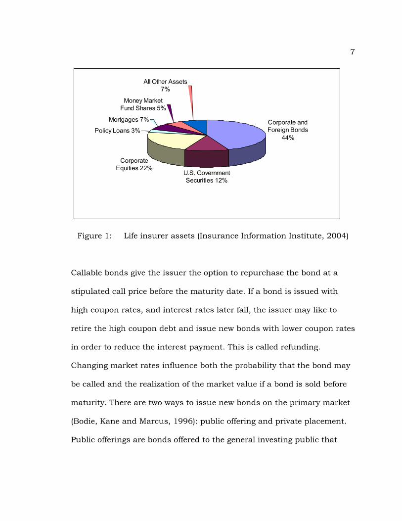
1.2.1 Assets and Liabilities of Life Insurers

An overview of the main categories of assets life insurance

companies hold in 2002 is given in figure 1. The chart is based on

numbers provided by the Insurance Information Institute (2004).

The largest investment category of life insurance companies are

corporate bonds. Publicly traded corporate bonds are characterized by

periodical coupons over their lives and the return of their face value to

the bondholder at maturity. Since private firms issue corporate bonds, it

is of real importance to consider the default risk. Most of the corporate

bonds contain options: the call option or the option to convert the bond.

Convertible bonds give bondholders the option to convert a bond into a

specified number of shares of common stock of the issuing firm. Thus,

the bondholder can profit from a positive development of the stock.

7

Mortgages 7%

Policy Loans 3%

Corporate Equities 22%

U.S. Government Securities 12%

Corporate and Foreign Bonds

44%

All Other Assets 7%

Money Market Fund Shares 5%

Figure 1: Life insurer assets (Insurance Information Institute, 2004)

Callable bonds give the issuer the option to repurchase the bond at a

stipulated call price before the maturity date. If a bond is issued with

high coupon rates, and interest rates later fall, the issuer may like to

retire the high coupon debt and issue new bonds with lower coupon rates

in order to reduce the interest payment. This is called refunding.

Changing market rates influence both the probability that the bond may

be called and the realization of the market value if a bond is sold before

maturity. There are two ways to issue new bonds on the primary market

(Bodie, Kane and Marcus, 1996): public offering and private placement.

Public offerings are bonds offered to the general investing public that

8

then can later be sold and purchased on the secondary market. A private

placement is issued to at most a few institutional investors. Generally,

the investor and the issuer directly negotiate the terms of the offering.

This and the fact that commissions are avoided are advantageous for

both sides, but it also contains risks. Many insurers obtain bonds

through private placements. But since a secondary market for private

placements does not exist, private placements are therefore generally

held to maturity. However, to offset the fact that they are less liquid and

marketable than public offerings, insurers expect an increased yield.

Investments in foreign securities have always been very small and

amount to approximately 5 percent of total assets. The major part of both

long-term and short-term non-U.S. corporate debt securities is invested

in Canadian securities by U.S. life insurers.

Life insurers hold large amounts of government securities, i.e.

Treasury securities and federal agency debts. Treasury securities are

obligations of the U.S. government issued by the Treasury to meet

government expenditures. Marketable Treasury securities can be

Treasury Bills, Treasury Notes and Treasury Bonds. Treasury Bills are

sold by the U.S. government in order to raise money. Any public investor

can buy them at the discounted face value of the Bill, and receives the

face value at the maturity date. They do not pay any coupons. The

9

maturities of Treasury Bills are up to one year. Treasury Bills are

considered the most marketable of all money market instruments. The

U.S. government also borrows money in large parts by selling Treasury

Notes and Treasury Bonds. Both provide semiannual coupon payments

at a level that enables the government to sell them at or near par value.

The maturities of Treasury Notes range from one year to 5 years, the

maturities of Treasury Bonds vary from 10 to 30 years. Treasury

securities are considered not to contain any credit risk and therefore

their expected yield is lower than that of corporate bonds or other fixed-

income securities.

Federal agency debts are securities issued by some government

agencies to finance their activities. If Congress believes that a sector in

the economy does not get sufficient credit through normal private

sources, then such agencies are created. The biggest part of this kind of

debt is issued in order to support farm credits and home mortgages.

Government securities are very liquid, which is advantageous if the sale

of assets is required due to cash flow changes.

Corporate equity, or common stock, holdings amount to 22 percent

of the total assets of life insurance companies. The total number refers to

both the general account and the separate account combined, but 90

percent of the stock held is in separate accounts. Black and Skipper

10

(2000) define the general account and the separate account as follows.

Life insurers divide their assets between two accounts: the general

account and the separate account. The general account is linked to

obligations with guaranteed, fixed benefit payments, like life insurance

policies. The separate account is directly associated with products that

pass the investment performance and risk to the policyholder, such as

variable life insurance and variable annuities. Therefore, the investment

in common stock in connection with separate account is not restricted.

Common stocks are ownership shares in a corporation and their cash

flows are therefore much more variable and riskier than those of fixed-

income securities. The market value of its shares and the non-

guaranteed, periodic payment of dividends account for the cash flows of

common stock. Common stock is also characterized by its residual claim

and limited liability. Residual claim means in case of liquidation the

stockholders are the last ones, after all other claimants, who are paid.

Limited liability means that the most they can lose is the money they

originally invested.

Life insurers invest less than 1 percent of their assets in preferred

stock. Preferred stock has characteristics of both equity and debt. It

typically promises to pay a fixed dividend each year, which must be

11

satisfied before common stock dividends can be paid. In this sense

preferred stock is similar to a perpetuity.

Policy loans comprise 3 percent of life insurer assets. Certain life

insurance policies allow policy owners to borrow money against the cash

value of their policy under conditions specified when the policy is written.

The accumulated cash value of a policy is defined by the total amount of

premiums paid, minus the cost of providing insurance protection for the

period of time since inception of the policy, plus interest or other benefits

accruing on previously paid premiums (Gardner and Mills, 1991).

Mortgages account for 7 percent of total assets of U.S. life

insurance companies. Mortgages are loans that require periodic

payments of principal and interest with real estate as collateral. A

residential mortgage refers to a one- to four family dwelling, whereas

commercial mortgages have commercial property, like an apartment

building (for more than four families) or a store, as collateral.

Commercial real estate mortgages generally are considered fixed-income

securities and illiquid investments. Since commercial mortgages are

directly negotiated between the insurer and borrower, and the liabilities

of life insurers typically are of long duration, mortgages were considered

to be an opportunity to match the cash flows. But because of augmenting

12

liquidity requirements, the mortgage loans tend to become closer to 10-

year maturities.

Policy reserves are by far the largest category of life insurance

liabilities. The prospective definition of the reserve is the amount that,

together with future premiums and interest earned, is needed to provide

future benefits based on current assumptions of mortality, morbidity and

interest (Black and Skipper, 2000). They are the difference between the

present value of future benefits and the present value of expected future

net premiums. The assumptions and the method of calculation vary with

different accounting standards. The valuation of annuity reserves is

based on the commissioners’ annuity reserve valuation method (CARVM)

defined in 1976. The present value of future guaranteed benefits at each

duration has to be compared to the present value of future required

premiums at that duration. The minimum reserve for the contract is the

present value of the greatest excess observed in these comparisons at the

valuation date.

A simple example of the commissioners’ annuity reserve valuation

method applied to a single-premium deferred annuity follows. It is

analogous to the example presented by Tullis and Polkinghorn (1996),

but all the values obtained here are based on my calculation. Consider

the annuity as described below:

13

Policy year Percent of fund

1 7%2 6%3 5%4 4%5 3%6 2%7 1%

8 and later 0%

Single premium: 10,000

No front end load

Guaranteed Interest: 9% in years 1 through 5

4% thereafter

Surrender charge:

Valuation interest rate: 8%

Death benefit equal to cash surrender value

First, the value of the fund accumulated at the guaranteed interest

rate and the cash value are calculated at the end of each of the first 10

policy years, as shown in table 1.

The present values at the date of issue and at the first four policy

anniversaries of each future cash value have to be calculated next, using

the valuation interest rate. The results are shown in table 2.

14

Policy year Fund Cash value

0 10,000 9,3001 10,900 10,1372 11,881 11,1683 12,950 12,3034 14,116 13,5515 15,386 14,9256 16,001 15,6817 16,642 16,4758 17,307 17,3089 17,999 17,99910 18,719 18,719

Table 1: Fund and Cash Values

(Source: Author’s Calculation.)

Table 2: CARVM Valuation

0 9,300 9,3001 10,137 9,386 10,1372 11,168 9,575 10,341 11,1683 12,303 9,767 10,548 11,392 12,3034 13,551 9,960 10,757 11,618 12,547 13,5515 14,925 10,157 10,970 11,848 12,795 13,8196 15,681 9,882 10,672 11,526 12,448 13,4447 16,475 9,613 10,382 11,212 12,109 13,0788 17,308 9,351 10,099 10,907 11,780 12,7229 17,999 9,004 9,724 10,502 11,343 12,25010 18,719 8,670 9,364 10,113 10,922 11,796

3 4

Cash value

Policy anniversary of valuationFuture policy year 0 1 2


15

For the first 4 years, the cash value, which creates the greatest present

value for valuations on each of the first four policy years, is the cash

value at the end of the 5th year. Hence, the CARVM reserve, for example

at the third policy year, would be 12,795, the present value of the fifth

policy year value.

Due to the nature of annuity reserving and the structure of

annuity policies, as opposed to life insurance, the largest single category

of reserves is for annuities. Pension fund reserves amount to 47 percent,

life insurance reserves comprise 29 percent of the total liabilities of life

insurance companies (Insurance Information Institute, 2004).

1.2.2 Assets and Liabilities of Property/Casualty Insurers

The investment policy of property/casualty insurance companies

can be described as follows (Feldblum, 1989). Long tailed liability lines,

such as general liability, products liability and medical malpractice, have

slow loss payout patterns and have gained importance in the last

decades. Since the investment risk on the assets that corresponds to

these loss reserves can not be passed to the policyholder, the insurers try

to match their investment and insurance portfolios. The ultimate liability

of a property/casualty insurer is generally not expressed in nominal

terms. It is determined at the settlement date, and hence depends on the

16

inflation between the accident and the settlement date. This means the

liabilities are inflation sensitive. Liabilities increase in case of rising

inflation rates, and decrease in case of falling inflation rates. In practice,

not all reserves are fully inflation sensitive. Often payments are

determined shortly after or at the accident date, and therefore have short

durations. But many reserves are inflation sensitive and therefore also

similar to short duration assets with regard to the consequences of

interest rate changes. Asset-liability matching or immunization, which

will be explained in depth in chapter II, requires an asset portfolio of the

same duration as the liabilities. Treasury Bills and commercial papers

are assets of short duration with returns varying directly with inflation.

But generally the yield curve is upward sloping, and therefore assets of

longer duration, like corporate bonds, provide higher yields. Thus, the

advantages of both immunization and the overall portfolio yield have to

be weighted. Common stocks are also inflation sensitive, as are

insurance liabilities, and change in the same direction, if the cash flows

resulting from current and expected dividends and from price changes or

expected dividend changes because of interest rate changes are

considered. If inflation and interest rates increase unexpectedly, common

stock prices decrease first, but increase later. But if common stocks are

reported at their market values their book values fluctuate more than

17

bonds. Therefore, long-term bonds are the primary choice of investment

for property/casualty insurers. Most insurers buy long-term bonds,

because higher yields can be expected. If long-term bonds are reported at

amortized values, they show high and steady returns. However, if they

are reported at their market values, long term bonds are risky assets

with regard to interest changes. In case of rising interest rates, the

market value of long-term bonds decreases. When interest rates fall, the

market value of bonds increases.

Figure 2, based on numbers provided by the Insurance

Information Institute (2004), shows the assets of property/casualty

insurance companies in 2002.

It is noticeable that their assets, compared to those of life

insurance companies, are dominated by municipal securities.

Property/casualty insurers invest 21 percent in municipal securities, 21

percent in corporate and foreign bonds and 18 percent of their assets in

U.S. government securities.

Municipal bonds are fixed-income securities issued by state or local

governments. There are two types of municipal bonds: General obligation

bonds are backed by the taxing power of the issuer. Revenue bonds are

issued, e.g. by airports, hospitals or port authorities, for financing special

projects. They are backed by the revenues of that project, and are

18

therefore riskier. The main reason why property/casualty insurers

choose this form of investment is that

Municipal Securities 21%

Corporate and Foreign Bonds

21%U.S. Government Securities 18%

Corporate Equities 17%

Trade Receivables 9%

Security Repurchase

Agreements 4%

Checkable Deposits and Currency 4%

All Other Assets 6%

Figure 2: Property/casualty insurer assets (Insurance Information

Institute, 2004)

interest income of municipal bonds is exempt from federal income taxes

(Bodie, Kane and Marcus, 1996). The interest income also is exempt from

state and local taxation in the state where the bond is issued. Capital

gains taxes, however, have to be paid at maturity or in case they are sold

19

at a value above the investor’s purchase price. Because of this tax-

exempt status, investors accept lower yields on these securities.

Maturities range from short-term tax anticipation notes to long term

municipal debt up to 30 years. But property/casualty insurers have to

consider both sides of investing in municipal bonds. In case of good

underwriting profits, the tax shelter that these bonds provide is

advantageous. In case of underwriting losses, the lower yield on

municipals hurts profitability.

17 percent of the assets are held in corporate equities. This is a

suitable investment for property/casualty insurance companies because

common stock is inflation sensitive, as are their liabilities. Theoretically,

the real value of the firm’s main assets should not change with inflation.

If inflation and interest rates rise, the nominal value of the firm should

consequently also rise, so that its inflation-adjusted value should not

vary. In practice, the value of a company is determined by its revenue

and costs. When inflation and interest rates increase, supply costs rise,

but demand may or may not. If inflation is “demand-pull”, i.e. a price

increase caused by an excess of demand over supply (Webfinance Inc.,

2004), demand increases. If inflation is “cost-push”, i.e. persistently

rising general price levels bought about by rising input costs (Webfinance

Inc., 2004), demand may decrease. Furthermore, households tend to

20

save and not consume more if interest rates rise, what further reduces

demand. Thus, the value of the firm and its common stock will decrease.

But when interest rates rise, investors often prefer to invest in long-term

bonds instead of common stocks to profit for a longer period of time from

the high rates. Hence, when inflation and interest rates increase

unexpectedly, common stock prices first decrease, but increase later, and

are therefore inflation sensitive.

Note that property/casualty companies do not segment funds, as

life insurers do. The investment returns of property/casualty insurers

have to be enough for the company as a whole, not for a certain block of

business (Feldblum, 1989).

Repurchase agreements are a form of short-term, generally

overnight, borrowing: a government security dealer sells securities to an

investor, in this case the insurance company, with an agreement to buy

back those securities by a specified date at a set price. The increase in

price is the interest gained (Bodie, Kane and Marcus, 1996).

A trade receivable is money owed to the insurance company,

whether or not it is currently due, as a result of a trade.

Property/casualty insurers generally make more use of short-term

investments than life insurers due to their liquidity needs. Trade

21

receivables amount to 9 percent, checkable deposits and currency to 4

percent, and security repurchase agreements to 4 percent.

Mortgages are not very attractive to property/casualty insurers

because of the completely taxable income from mortgage loans and

because of its illiquidity (Gardner and Mills, 1991).

If surrender, withdrawals or policy loans entail cash outflows, a

company risks losses if assets have to be sold at depressed prices at a

time when interest rates have increased. This risk is called

intermediation risk and is faced by life insurers (Atkinson and Dallas,

2000). But since property/casualty insurers do not loan to policyholders

and offer mostly short-term policies, they do not face disintermediation

problems.

The liabilities of a property/casualty insurance company primarily

consist of reserves. Reserves can mainly be separated into three parts:

the loss reserves, the unearned premium reserves and the loss

adjustment expense reserves.

The loss reserves are the largest portion of the liabilities. They have

been incurred because of claims that have been made but not yet paid.

Because estimated losses of property/casualty insurers are not based on

mortality and morbidity, they often rely on past experience, with

adjustments to reflect increased costs due to inflation or other factors. If

22

an insurer’s loss reserves are overestimated, the insurer’s profits will

decrease, the income taxes may be reduced, and premium rates may be

unnecessarily increased. If reserves are too low, underwriting profits will

be overstated, income taxes will increase, and premium rates may be cut

unwisely. In both cases, the insurance company will have lower than

optimal profitabililty.

Unearned premium reserves are obligations for the unexpired

terms of new and renewed policies to policyholders who have paid

premiums in advance.

The loss adjustment expense reserves contain the fees or salaries

paid to claims adjusters, fees paid to investigators, their expenses, e.g.

for traveling, legal fees, and other costs associated with settling claims

(Cohen and Mooney, 1991).

1.3 Valuation

Valuation informs about the financial condition and current

operating results of an insurance company. It measures and compares

the insurer’s assets and liabilities due to valuation standards, such as

interest rates, mortality, morbidity, persistency and expense

assumptions. These standards were created by the National Association

23

of the Insurance Commissioners (NAIC) and adopted by each state’s

legislature (Atkinson and Dallas, 2000).

Two different valuation principles are required for every insurance

company: statutory accounting and tax-basis accounting. If the

insurance company is publicly traded, GAAP accounting is also

obligatory. But since these principles are not sufficient for management

decisions, most insurance companies also use managerial accounting.

The state insurance law requires the use of statutory accounting

principles (SAP) in order to analyze a company’s ability to meet its

obligations to policy owners. The insurer must annually present financial

statements that both proof the economic solvency and the statutory

definition of solvency with regard to investments, reserves, and minimum

capital and surplus defined by law. The insurer must prove that its

assets, future premiums and conservatively estimated interest income

will be enough to meet all promises to policy owners. Profits on existing

or new lines of business are not considered.

The usefulness of statutory reports is restricted for two reasons.

First, results are reported at a specific point in time under some static

assumptions that neglect possible changing economic conditions in the

future. However, a NAIC model law requires the proof of an adequate

reserve for various economic scenarios. Because traditionally most

24

insurers held bonds to maturity and did not even intend to sell them

earlier, bond values are recorded at amortized values rather than market

values. During periods of relatively high interest rates, the asset values

are overestimated and artificially stabilized by these amortized values.

Thus, it is possible that the insurer’s statement shows solvency whereas

the insurer actually is not able to meet his future obligations, and vice

versa.

Second, statutory accounting is not adequate for investors and

creditors, because it is balance sheet oriented and treats the insurer as if

he were about to be liquidated. Additionally, the use of conservative

assumptions used for the valuation of the insurer’s liabilities generally

neglects the possible profit that can be generated by in-force policies in

the long run.

The use of generally accepted accounting principles (GAAP) is

required by the Securities and Exchange Commission for publicly traded

insurance companies and is a condition for listing on major stock

exchanges. The main purpose of GAAP accounting is to report the

financial results for an insurance company such that it is comparable to

those of other companies and of other reporting periods. This

comparability is particularly important to investors in order to judge

25

alternative investment possibilities and to predict future financial

results.

Although GAAP accounting presents assets, liabilities and cash

flows, it does not recognize possible future profits generated by existing

and future policies. Therefore it is not appropriate to evaluate the long-

term financial impact of current management action, and hence it is

often considered not to be adequate as a financial management tool.

More detailed, GAAP includes the lock-in principle, which does not

allow restating the assumptions of interest, expense, and mortality for

traditional policies in force. Only interest-sensitive products and

participating business can periodically be reevaluated. Furthermore,

unrealized capital gains and losses are not reflected in the GAAP income

statement. Finally, GAAP as well as SAP, do not recognize the future

impact of current events, since surrenders may cause increased current-

period earnings, and do not reflect the loss of future profits on lapsed

policies.

The main difference in SAP and GAAP accounting concerning the

valuation of assets is the distinction between admitted and non-admitted

assets. Assets approved by state regulatory authorities and accepted by

the NAIC Annual Statement are called admitted assets. These are rather

liquid assets, such as bonds, stocks, mortgages and real estate. Non-

26

admitted assets are usually either illiquid, e.g. furniture and equipment,

or not allowed by statute, e.g. certain kinds of securities above the

statutory limit. Only admitted assets may be listed on the statutory

balance sheet. However, on the GAAP balance sheet, all, i.e. both

admitted and non-admitted assets, may be reported. Roughly, SAP

reports only admitted assets and those at amortized values, while GAAP

recognizes all assets at market values.

As far as the valuation of liabilities is concerned, the

property/casualty situation is much different from the life insurance

case: Property/casualty insurers report both statutory and GAAP

reserves at undiscounted values. Whereas the valuation of statutory

reserves for life insurers is defined by law and the valuation of GAAP

reserves is based on the company’s and industry’s experience (Black and

Skipper, 2000).

Generally, GAAP recognizes liabilities later or at a lower value and

recognizes assets earlier or at a higher value. GAAP accounting treats the

business more as a going concern, whereas SAP accounting rather treats

it as if it were about to be liquidated.

The third valuation principle, the tax-basis accounting, is required

by the Internal Revenue Service. It necessitates the calculation of the

reserve liability in order to determine the taxable income in accordance

27

with the Internal Revenue Code and its interpretations (Atkinson and

Dallas, 2000).

Since all three regulatory accounting principles do not properly

represent the performance of lines of business adequately for

management decisions, most insurers have adopted management-basis

accounting (Dicke, 1996). These three principles do not completely

recognize the following issues either:

• Changes in present value of cash flows according to changes in

interest rates

• Embedded options in assets and liabilities

• Lost future profits due to surrenders or additional profits due to

new sales in the long run

• Expected future profits on future business

• Actual market values of assets held in the investment portfolio

These deficits resulted in the development of economic value

analyses, which is now often used in insurance firm management. The

most essential ones are the value-added and return-on-equity methods.

28

1.4 Risks

Most insurance companies identify and manage the risks they face

according to the classification developed by the Society of Actuaries

(Ostaszewski, 2002):

• Asset default (C-1) risk: is the risk of a decrease in the

insurer’s investment asset value. It can either be caused by

the default of borrowers in payment of interest or principal,

or by declining market values of assets (if not based on

interest rate movements).

• Insurance pricing (C-2) risk: is the risk of losses from

increasing claims and pricing deficiencies. The latter may

occur if the actual mortality, morbidity, lapse or expense

experience is higher than the expected, i.e. if future results

do not match the assumptions implicit in product pricing.

• Interest rate (C-3) risk: is the risk that changes in interest

rates affect assets and/or liabilities in a negative way. This

will be discussed more detailed in the next chapter.

• Business (C-4) risk: represents miscellaneous risks that are

not mentioned in C-1 through C-3, e.g. market risk from

29

expansion into new lines of business, changes in taxation or

regulation, insurance fraud, mismanagement and law suits.

The primary concern of early insurance companies was the C-2

risk, since they were not able to predict their benefit disbursements. But

with the development of the principles of actuarial sciences the

importance of the C-2 risk gradually decreased. In the 1950s and 1960s

almost all claim-related cash flows were known. And also other cash

flows, such as lapses, surrenders, new business or investment returns,

were stable and therefore predictable (Ostaszewski, 2002). Since interest

rates stayed in a narrow range from the Great Depression until the mid-

1960s – the yield on long-term U.S. government securities e.g. stayed

between 2 and 4.5 percent – they were not problematic either. This stable

environment ended in the 1970s when inflation accelerated and became

unpredictable, and the volatility of financial markets, especially interest

rates, increased. In the early 1980s, the short-term interest rates were at

unprecedented height. High rates combined with greater volatility

encouraged more and more individuals to borrow against their life

policies and reinvest the proceeds at higher rates elsewhere.

Policyholders changed their behavior with regard to the options

30

embedded in their contracts. They started to exercise the options more

frequently and opportunistically.

Some examples of options embedded in insurance policies are (Laster

and Thorlacius, 2000):

• Settlement option: allows the beneficiary the choice of the form of

benefit payment, e.g. lump sum or annuity.

• Policy loan option: offers the policyholder the right to borrow, at

specified terms, against the accumulated asset value of an

insurance policy.

• Over-depositing option: enables the policyholder to pay higher

premiums than required, which will be credited at a pre-specified

interest rate.

• Surrender privilege: permits the policyholder to stop paying

premiums and to halt the insurance contract earlier.

• Renewal privilege: allows policyholders to continue an insurance

contract or halt the agreement at the end of the policy period.

When interest rates were stable, these options were not very

valuable. Hence, many insurers did not adjust their assets and liabilities

31

and were therefore not prepared for the risks these options posed when

interest rates became volatile.

In the mid 1980s, the level of nominal interest rates declined

dramatically and as a consequence, many insurers’ portfolios were

refinanced and prepaid. At the end of the 1980s, insurers that followed

higher yields often took too much credit risk in their investment portfolio.

Another response to high interest rates and increased competition

at the end of the 1970s was the rise of new, interest-sensitive policies.

Annuities were historically not an important part of life insurance

industry and just used as a source of income after retirement. But

annuities gained more importance than traditional insurance, since the

main purpose of purchasing life insurance was no longer protection but

investing. Single, flexible premium-deferred annuities, variable annuities,

universal life and other interest-sensitive products exposed insurers to

new sorts of risk that some have not been able to manage. As a

consequence, the National Association of Insurance Commissioners

adopted an Amendment to the Standard Valuation Law in 1990. It

required a basic asset-liability analysis, known as cash flow testing, to

verify that the insurer holds enough reserves. Thereby, the effects of

various different interest scenarios on the assets and liabilities are

tested.

32

Thus, these changes simultaneously caused the relative decline of

the C-2 risk, except for the catastrophe risk of property/casualty

insurance companies, and the increase in the significance of the C-1 and

C-3 risk.

33

CHAPTER II

INTEREST RATE RISK

The term C-3 or interest rate risk denotes the risk of losses

because of changes in interest rates – changes in either the level of

interest rates or the shape of the yield curve.

In order to understand what this means, consider a block of

insurance business and its associated assets. The asset cash flow in any

future time period consists of the investment income and capital

maturities (principal repayments) expected to occur in that time period.

The liability cash flow in any future period consists of the policy claims,

policy surrenders and expenses minus the premium income expected to

occur in that time period. Therefore the net cash flow is the difference

between the asset cash flow and the liability cash flow. If the net cash

flow is positive, the asset cash flow exceeds the liability cash flow, which

generates excess cash for (re)investment. If interest rates are below the

initial rates when the net cash flows are positive, the cash flows may

have to be reinvested at lower rates and thus losses may occur. This is

34

related to as reinvestment risk. On the other side, negative net cash flows

denote shortages of cash needed to meet liability obligations. In this case

assets have to be liquidated or borrowed (within or without the

company). If interest rates are above the initial level when the net cash

flows are negative, losses can occur due to the fact that bonds and other

fixed-income securities whose values have fallen must be liquidated. This

is called disinvestment risk or price risk. The various interest rate options

embedded in the assets and liabilities further aggravate the C-3 problem;

this means that both the asset and the liability cash flows are functions

of interest rates. When interest rates rise, more policyholders are

expected to surrender their policies (to obtain higher returns by

reinvesting the cash values elsewhere) or make use of their policy loan

options. On the other side, when interest rates decline, bonds are more

likely to be called, and bonds can be prepaid earlier than expected (Shiu,

1993).

Important measures of interest rate risk are duration and

convexity. These two concepts are essential tools for asset-liability

management.

35

2.1 Duration

Both duration and convexity are based on the assumption that

only one interest rate is used, which means we assume a flat yield curve.

Hence we examine the sensitivity to small parallel shifts in the yield

curve, not bends or twists in rates.

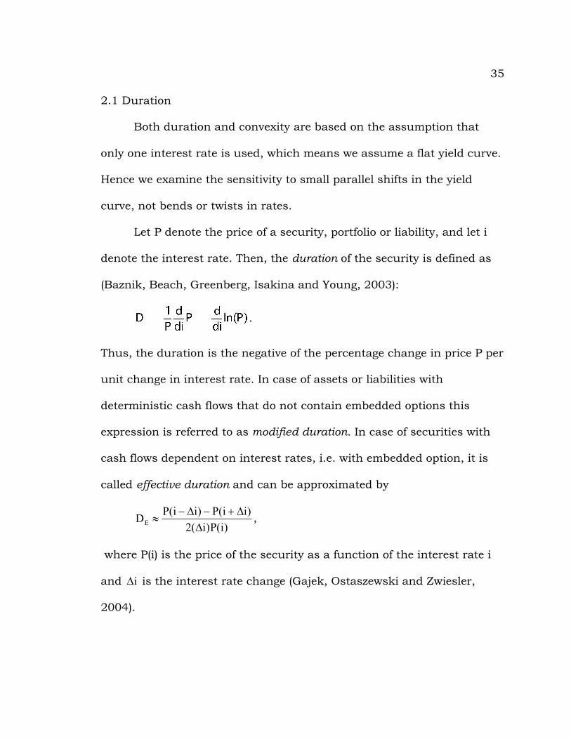
Let P denote the price of a security, portfolio or liability, and let i

denote the interest rate. Then, the duration of the security is defined as

(Baznik, Beach, Greenberg, Isakina and Young, 2003):

.

Thus, the duration is the negative of the percentage change in price P per

unit change in interest rate. In case of assets or liabilities with

deterministic cash flows that do not contain embedded options this

expression is referred to as modified duration. In case of securities with

cash flows dependent on interest rates, i.e. with embedded option, it is

called effective duration and can be approximated by

)i(P)i(2

)ii(P)ii(PDE DD+-D-

» ,

where P(i) is the price of the security as a function of the interest rate i

and iD is the interest rate change (Gajek, Ostaszewski and Zwiesler,

2004).

36

A positive duration means that when interest rates increase, the

price of the instrument decreases, which is the case for most fixed-

coupon, fixed-income instruments and for liabilities with reasonably

well-defined cash flows. Negative duration means that the price of the

instrument will increase when the interest rate increases.

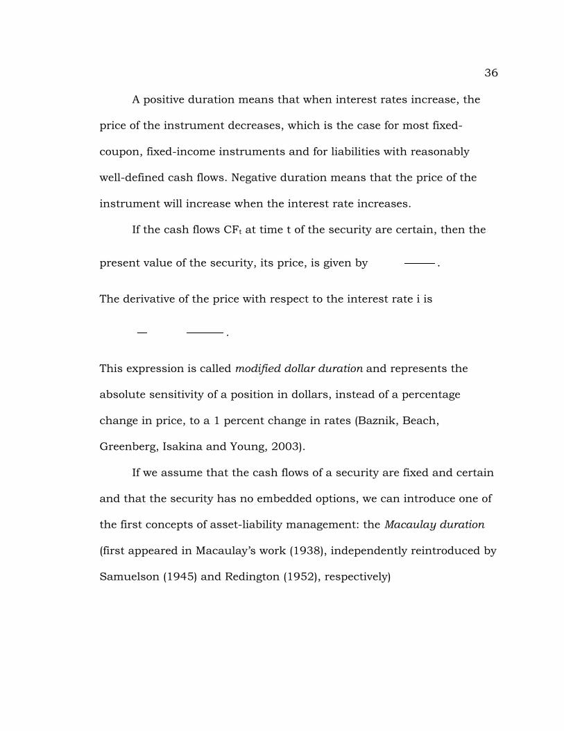
If the cash flows CFt at time t of the security are certain, then the

present value of the security, its price, is given by .

The derivative of the price with respect to the interest rate i is

.

This expression is called modified dollar duration and represents the

absolute sensitivity of a position in dollars, instead of a percentage

change in price, to a 1 percent change in rates (Baznik, Beach,

Greenberg, Isakina and Young, 2003).

If we assume that the cash flows of a security are fixed and certain

and that the security has no embedded options, we can introduce one of

the first concepts of asset-liability management: the Macaulay duration

(first appeared in Macaulay’s work (1938), independently reintroduced by

Samuelson (1945) and Redington (1952), respectively)

37

,

where CFt are the certain cash flows, the price P is the present value of

the discounted cash flows , and i is the interest rate used to

discount them (Gajek, Ostaszewski and Zwiesler, 2004).

The Macaulay duration can be expressed in terms of the interest rate i

(as shown above) or in terms of the force of interest δ, since d=+ ei1 and

therefore i1did

+=d :

åå

³

×d-³

×d-×=

d-=

d-=

0tt

t0t

tt

M CFe

CFetP

dd

P1)Pln(

ddD .

Note that åå³

×d-

³

=+

=0t

tt

0tt

t CFe)i1(

CFP is still the present value of the security.

The Macaulay duration can be interpreted as the weighted average time-

to-maturity of the security’s cash flows, where the weights are the

present values of each cash flow. In the special case of a non-callable,

default-free, zero-coupon bond, the Macaulay duration is always the time

to maturity.

There are some more characteristics of the Macaulay duration that

are worth mentioning. First, if the maturity increases, the Macaulay

38

duration also increases. But because of the use of the present value in

its calculation the Macaulay duration increases more slowly than does

maturity. Second, if the interest rate increases the duration decreases.

This makes sense since discounting at higher interest rates has a greater

effect on later cash flows and their relative importance declines. Third,

higher coupon or interest payments yield to a lower Macaulay duration.

This is understandable; if the payments at the beginning are larger, the

cash flows are received earlier and the present value weights of those

cash flows are higher.

2.2 Convexity

Convexity (Baznik, Beach, Greenberg, Isakina and Young, 2003) is

a second order term and measures the change in price from the duration

estimate for a small change in interest rates. If an instrument has

positive duration and no embedded options, positive convexity means

that the duration gets longer when interest rates fall, and the duration

shortens when interest rates rise. This is the case for fixed cash flow

bonds. Securities with embedded options may have regions with negative

or reduced positive convexity. For example, home mortgages may have

negative convexity as rates lower and increase the likelihood of

prepayments, which results in lower duration as rates fall. Convexity

39

may turn positive from lower likelihood of prepayment or extension, and

result in greater duration as rates rise.

The Macaulay convexity of a security with certain cash flows tCF at

time t and price å³

×d-=0t

ttCFeP is the convexity measure with respect to the

force of interest d (Gajek, Ostaszewski and Zwiesler, 2004):

åå

³

×d-³

×d-

×

××=

d=

0tt

t0t

tt2

2

2

M CFe

CFetP

dd

P1C .

It indicates the sensitivity of the duration measure with respect to

changes in the force of interest.

Because PddDP M d

-=× , where MD is the Macaulay duration,

we have

PddP

dd

P1

P1

ddDP

ddDD

ddP

P1)DP(

dd

P1C M

MMMM dúûù

êëé

d--

d-=úû

ùêëé

d+

d-=×

d-=

2M

MM DddDP

dd

P1P

dd

P1

ddD

+d

-=dd

+d

-= .

The quantity 2MM

M2M DC

ddDM -=d

-= will be termed Macaulay M-squared.

The Macaulay M-squared can be seen as a measure of dispersion of the

cash flows of the security. The Macaulay convexity is the sum of the

Macaulay M-squared and the square of the Macaulay duration. This

40

means that the more dispersed the cash flows are, or the longer the

duration cash flows are, the greater the convexity (Ostaszewski, 2002).

For a zero-coupon bond maturing in T years, the Macaulay convexity is

2T . Since the Macaulay duration is T, the 2MM of this zero-coupon bond

is 0TTM 222M =-= .

For assets or liabilities with embedded options the effective

convexity can be approximated by the following expression:

)i(P)i(

)ii(P)i(P2)ii(PC 2E DD++-D-

» ,

where P(i) is the price of the security as a function of the interest rate i,

and iD is the change in the interest rate.

2.3 Immunization

The British actuary Frank M. Redington coined the term

“immunization” in his 1952 paper “Review of the Principles of Life-Office

Valuations” (Redingtion, 1952). His paper intended to be about valuation

rather than strategies for matching assets and liabilities. In this paper,

he proposed the use of a similar basis for the valuation of both assets

and liabilities. He suggests the equation of the mean term of assets to

that of the liabilities, while a greater spread for the cash flows of the

assets is required in order to immunize the surplus value of a block of

41

business against interest rate changes. Redington’s idea of mean term

had already occurred in the work of Frederick R. Macaulay (1938), and

his term “duration” is the one generally used today (Panjer, 1998).

Macaulay’s duration is the main concept used in Redington’s theory of

immunization.

Consider a block of long-term insurance or annuity policies and its

related assets at time 0t = . Let tA be the asset cash flow expected to

occur at time t: interest income, dividends, rent, capital maturities,

repayments and prepayments. Let tL be the liability cash flow expected

to occur at time t, i.e. policy claims, policy surrenders, policy loan

payments, policyholder dividends, expenses, and taxes, less premium

income, policy loan repayments, and policy loan interest. Let the assets

be more dispersed than the liabilities, i.e. choose assets with greater

convexity than the liabilities. Redington argues that the same interest

rate i should be applied to discount both the asset and liability cash

flows to figure out their values, since every insurance liability cash flow

can be considered the negative of an asset cash flow. Let i denote the

given interest rate. Then the present values of the assets and liabilities

are the sums

å³ +0t

tt

)i1(A and å

³ +0tt

t

)i1(L .

42

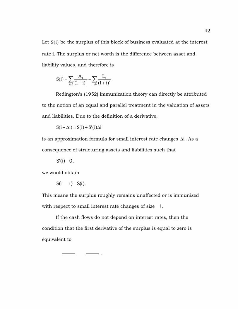
Let )i(S be the surplus of this block of business evaluated at the interest

rate i. The surplus or net worth is the difference between asset and

liability values, and therefore is

åå³³ +

-+

=0t

tt

0tt

t

)i1(L

)i1(A)i(S .

Redington’s (1952) immunization theory can directly be attributed

to the notion of an equal and parallel treatment in the valuation of assets

and liabilities. Due to the definition of a derivative,

i)i('S)i(S)ii(S D+»D+

is an approximation formula for small interest rate changes iD . As a

consequence of structuring assets and liabilities such that

,

we would obtain

.

This means the surplus roughly remains unaffected or is immunized

with respect to small interest rate changes of size .

If the cash flows do not depend on interest rates, then the

condition that the first derivative of the surplus is equal to zero is

equivalent to

.

43

This tells us that the first moment of the asset and liability cash flow

streams are equal, which forms the fundamental of Redington’s

immunization strategy. If the present value of the assets additionally

equals the present value of the liabilities, this means the Macaulay

durations of the assets and liabilities are matched; the changes in asset

values will be exactly offset by the changes in liability values.

The deficiency of this model is that it allows arbitrage

opportunities. To see why, we use the three-term Taylor approximation

formula (Panjer, 1998)

.

If both the conditions

and

are satisfied, then, for small changes in the interest rate, this results in

.

Thus, changing interest rates always imply an automatic increase in

surplus. This automatic “free lunch” in the model results from the use of

the same interest rate applied to discount all cash flows. The model

always assumes a flat yield curve, i.e. it does not distinguish between

short- and long-term interest rates (Panjer, 1998).

44

Immunization also assumes the knowledge of all future asset and

liability cash flows. However, in reality the future cash flows, especially of

an insurance company, are hard to predict with regard to both their

values and timing.

Moreover, Macaulay duration explicitly assumes deterministic cash

flows. Thus it can not meaningful be used in cases where cash flows may

depend on interest rates. But this is true for assets and liabilities that

contain embedded options; policy owners may surrender their policies

when interest rates rise, bonds may be called and mortgages repaid when

interest rates fall and so on, as discussed earlier. In this case, the

concept of option-adjusted duration and option-adjusted convexity (also

called effective duration and effective convexity) should be applied

(Ostaszewski, 2002).

Another difficulty with this approach is that duration varies with

interest rate movements and over time. Even if the duration of the assets

and liabilities has initially been matched, their durations might differ

once the interest rate shifts. As a consequence, immunization requires

continuous rebalancing of the assets and liabilities. Since convexity

measures how rapidly duration changes in response to a change in

interest rates, matching both durations and convexities is also

45

advantageous. This way, an insurer hedges its interest rate risk to a

second degree of precision (Laster and Thorlacius, 2000).

A further aspect is the question why a company should pursue a

strategy where it minimizes its surplus. If both

and

hold true, this means that the surplus function has a local minimum at

the current level of interest, and every small change in the interest rate

adds surplus. As it turns out immunization in practice pursues the point

of maximum wealth and rather maximizes interest rate risk


The strength and weakness of the traditional immunization

strategy resulted in the development of all the modern techniques of

asset-liability management.

2.4 Yield Curve and Multivariate Immunization

In the preceding chapters, we used only one interest rate to

discount the cash flows of all maturities. However, in reality the interest

rates for discounting cash flows for different maturities are not the same.

The yield curve, or term structure of interest rates is the pattern of

interest rates for discounting cash flows of different maturities. The yield

curve generally represents the functional relationship between the time to

46

maturity and the corresponding interest rate, whereas term structure of

interest rates usually describes the fact of interest rates varying for

different maturities. If longer-term bonds offer higher yields, which is

generally the case, the yield curve is said to be upward sloping. If interest

rates for various maturities do not differ, we call this a flat yield curve.

And if shorter-term maturity interest rates are higher than longer-term

rates, which occurs rarely, the pattern is called inverted yield curve. In

practice, estimates of the yield curve are based on Treasury Bills,

Treasury Notes and Treasury Bonds, since they are considered to be risk-

free. Actually, there are three ways to define the yield curve. The first one

is called bond yield curve and assigns to each maturity the coupon rate

of a (generally newly issued) bond of that maturity trading at par. The

second one is called spot curve. It assigns to each maturity the interest

rate on a zero-coupon bond of this maturity. This interest rate is called

spot rate. The third definition of the yield curve applies short-term

interest rates in future periods of time implied by current bond spot

rates. A short-term interest rate or short rate represents an interest rate

that is used for a short period of time, i.e. for an instantaneous rate over

the next infinitesimal period of time or a period of time up to one year.

Applying the one-year rate as the short rate, we can derive forward rates

and the relationship between these two:

47

)f1)...(f1)(f1()s1( n21n

n +++=+ ,

where ns is the spot rate for maturity n and if is the forward rate from

time 1i - until time i, n,...,1i = .

We also have

1n1n

nn

n )s1()s1(f1 -

-++

=+ .

The yield curve can also be defined for continuously compounded

interest rates, i.e. for the force of interest. Here, the force of interest

t)t( d=d=d is a function of time. To explain the difference between the

spot force of interest td for time t and the forward force of interest tj at

time t, their mathematical relationship is presented. The accumulated

value at time t of a monetary unit invested at time 0 is

ò

=j

d

t

0s

t

dst e)e( .

Thus we have ò j=dt

0st ds

t1 , which means the spot rate for time t is the

mean value of the forward rates between 0 and t (Gajek, Ostaszewski,

Zwiesler, 2004).

To remove one weakness of the traditional immunization theory,

Ho (1990) and Reitano (1991a, 1991b) generalize duration and convexity

to the multivariate case. Instead of using one single interest rate

48

parameter i, a yield curve vector )i,...,i(i n1=®

is used, where the

coordinates of this vector refer to certain “key” rates, e.g. based on

observed market yields at various maturities. Then, the price )i,...,i(P n1 of

a security is a function of these key rates. We implicitly assume that they

are independent, i.e. each of them has its derivative with respect to the

other equal to zero. But this is certainly not the case for various maturity

interest rates.

The negative partial logarithmic derivatives of )i,...,i(P n1 are called

partial durations (Reitano, 1991a, 1991b), or key-rate durations (Ho,

1990). The total duration vector then is

÷÷ø

öççè

æ¶¶

¶¶

-=-n1n1n1

n1

iP,...,

iP

)i,...,i(P1

)i,...,i(P)i,...,i('P .

The second derivative matrix defines the total convexity:

nl,k1lk

2

n1n1

n1

iiP

)i,...,i(P1

)i,...,i(P)i,...,i("P

££úû

ùêë

é¶¶

¶-=- .

The surplus S of a company can be expressed in terms of the key

interest rates chosen: )i(S)i,..,i(SS n1

®

== . Analogous to the one-

dimensional case, the multivariate immunization can be applied using

multivariate calculus. To protect the surplus level from changes in

interest rates, the first derivative has to be set equal to zero

49

®®

=÷÷ø

öççè

æ¶¶

¶¶

= 0iS,...,

iS)i('S

n1

,

and the second derivate matrix has to be made positive definite (Gajek,

Ostaszewski, Zwiesler, 2004).

50

CHAPTER III

STRATEGIES AND TECHNIQUES FOR


An overview of the strategies and techniques for asset-liability

management is provided by Van der Meer and Smink (1993). They

present both simple methods and methods applying more difficult

theories from finance or actuarial science. Further, they explain the basic

benefits and weaknesses.

The analyzed strategies and techniques can be classified in two

groups: static and dynamic. Since strategies necessitate rules that

specify how to make decisions they are considered dynamic, whereas

techniques are considered static.

3.1 Static Techniques

The static techniques are ordered at increasing level of

sophistication. Most of the methods are commonly applied in banking

and insurance. The reason therefore might be the fact that they are

51

relatively easy to understand and implement. These methods concentrate

on a complete match between assets and liabilities, especially in the case

of cash flow matching. The usefulness of these approaches is limited as

they do not consider the possibility of a consistent trade-off between risk

and return. Risk and return are not explicitly measured by these

techniques. Moreover, those methods are based on the assumption of

complete predictability of cash flows, which makes them not very useful

for insurance companies, especially not for property/casualty insurers

whose liability reserves are inflation sensitive (Ostaszewski, 2002).

• Cash flow payment calendars:

Cash flow payment calendars provide an overview of all cash

inflows and cash outflows of a company. It is a tool for identifying

main imbalances between cash flows that result from assets and

liabilities.

• Gap analysis:

Gap analysis is routed in bank asset-liability management. The

gap is defined as the difference between the values of the fixed and

variable rate assets and liabilities on the balance sheet.

Maintaining a gap as close to zero as possible is a risk-minimizing

stratgey, a non-zero gap indicates interest rate risk exposure. For

52

example, when the variable rate assets exceed the liabilities, then

decreasing rates will result in a loss in net operating income. More

helpful than pure gap analysis is a refined version that accounts

for maturity differences between assets and liabilities, i.e. the

company’s asset and liability categories are classified according to

when they will be reprised and when they will be placed in

groupings called time buckets.

• Segmentation:

Segmentation is a method used by insurance companies. For this

method, liabilities are partitioned due to differences that result

from product characteristics. Then, a separate asset portfolio is

assigned to each segment, which has to reflect the particular

structure of the liabilities, e.g. concerning the cash flow pattern.

• Cash flow matching:

Cash flow matching is a technique that intends to minimize the

imbalances between all asset and liability cash flows, generally

using the method of linear programming. The scheduled negative

cash flows generated by the liabilities are projected and an asset

portfolio that generates the same cash flows is selected. The asset

portfolio has to match the liabilities with certainty, within a very

53

small acceptable time span, and with minimal cost (Ostaszewski,

2002).

Cash flow matching may cause several practical problems.

First, it is not always possible to match the liability cash flows

completely, e.g. in case the liability cash flows have very long

maturities and corresponding assets are not available in the

market. Second, a complete cash flow match may be too restrictive

for managing the portfolio since it does not consider the higher

return, which results from undertaking a higher degree of risk. But

this is especially important for highly priced liabilities whose

associated costs have to be regained by the asset portfolio. Finally,

this technique supposes a complete and exact knowledge of the

timing and value of all cash flows, whereas this is often not

possible. For example if the cash flows depend on interest rates or

other stochastic factors, cash flow matching is not achievable for

all possible future scenarios.

Multiscenario analysis is not a purely static technique (Van der

Meer and Smink, 1993). Since it forms a link between the static

techniques presented and the dynamic strategies, it is mentioned here.

The projected development of the cash flows of the liability and the asset

54

portfolios is the focus of multiscenario analysis. These projections are

made under varying future scenarios with regard to interest rates,

inflation and other variables that are in part responsible for

dependencies between assets and liabilities. The analysis reveals under

which scenarios cash flows are not matched and what the consequences

are for the company. Multiscenario analysis gives a deeper insight into

the different sorts of risks the company faces, but the user tends to be

biased towards scenarios which seem to be more likely, while other

scenarios may be more distressing. This may also be the case if scenarios

are randomly generated.

3.2 Dynamic Strategies

The second group of asset-liability management strategies, the

dynamic strategies, can be classified in value driven and return driven

methods. The methods of both categories explain the relationship

between assets and liabilities, and other factors that have an influence

on their balance.

3.2.1 Value Driven Dynamic Strategies

The value driven dynamic strategies are all based on Redington’s

(1952) classical notion to protect the company’s surplus from interest

55

rate risk. With regard to the identified pitfalls of his immunization

strategy solutions have been provided for some cases and several

modified immunization strategies have been developed. But they still

have the goal to dynamically replicate a risk free asset, i.e. to preserve

the surplus value.

Further, they can be divided into two groups: passive and active

value driven dynamic strategies. Passive value driven dynamic strategies

are:

• Immunization:

The immunization (also called standard immunization) principle

involves duration matching and is discussed in the preceding

chapter.

• Model conditioned immunization:

The model conditioned immunization drops the assumption of a

flat yield curve and modifies the standard immunization theory by

using a stochastic process that determines the development of the

yield curve over time. The process that determines the development

can depend on one or more factors. In case of the single factor

immunization, only the short term interest rate is defined by a

stochastic process, and the long term structure of interest rate is

56

defined as by Cox, Ingersoll and Ross (1985). In case of the multi-

factor immunization, a limited number of independent factors

determines the shape of the term structure. Such factors can for

example be observed forward rates or the long term average of the

short term rate. The sensitivities to changes in the yield curve can

be defined by model specific durations. The immunization concept

used is the same as in the standard immunization theory. The

model conditioned immunization strategies only differ with respect

to the duration and convexity measures applied.

The advantage of these strategies is their possible precision

and the chance to integrate derivative instruments in the same

term structure environment. The main disadvantage is the non-

stationarity of factors. This may result in a risk related to the

validity of the model and may necessitate monitoring these factors.

• Key rate immunization:

Key rate immunization is very similar to standard immunization

except that it allows non-parallel term structure shifts. Instead of

using one interest rate i, a limited number of key interest rates

n21 i,...,i,i are used, which shape the term structure and which can

be interpolated to determine the other values. Thus, the price P of

a security will be a function of several variables:

57

.

Since we may have different changes in interest rates ,

key rate immunization requires to equate the corresponding sets of

partial derivatives of to those of


The active immunization strategies intend to guarantee a minimally

acceptable level of surplus while allowing active asset portfolio

management in order to achieve higher asset returns. They also

implicitly assume that a positive surplus is available.

• Contingent immunization:

Contingent immunization was developed by Leibowitz and

Weinberger (1982, 1983). It allows active portfolio management

while meeting the requirements of portfolio matching. The main

idea is the immunization of the asset portfolio at any point in time.

While the asset portfolio exceeds the amount needed to meet the

liabilities, the asset portfolio can be managed actively in order to

attain better performance. But if the asset portfolio drops to a

specified minimum value, the portfolio has to be managed through

an immunization strategy.

58

• Portfolio insurance:

Using the option pricing theory and the derivation of the Black-

Scholes option pricing formula, Leland and Rubinstein (1981)

developed a strategy of replicating an option on a capital asset. It

permits possible gains from asset investments, but preserves the

portfolio value above or at a specified level.

Ostaszewski (2002) describes this in depth. A European call is the

right to buy a security at a predetermined price at some future

point in time. A European put is the analogous right to sell a

security. Let C denote the price of the European call, and P denote

the price of the European put, both with exercise price X in time T

in the future. Let the capital asset be S and assume it does not

provide any dividend or other sort of income. A portfolio consisting

of one unit of capital asset S and one put P on that capital asset

will have a terminal value of S if XS ³ or of X if SX ³ at time T. But

if we have a portfolio of a call C on one unit of capital asset and

cash that will, together with the interest earned at the risk-free

rate, equal the present value of the exercise price PV(X), then the

portfolio will have the same value at time T as the portfolio

described before:

PS)X(PVC +=+ .

59

This is called put-call parity (Panjer, 1998) and describes the

relationship of a portfolio of cash and capital asset to a portfolio of

call and put, since the equation can be rearranged to

PC)X(PVS -=- .

The payoff of the portfolio consisting of cash in the amount of PV(X)

and the call will be the same as the one of the portfolio presented

first, if we use the following strategy: If between now and time T the

price of the capital asset is above PV(X), keep the capital asset. If

the price drops to PV(X), sell the asset and keep the cash. If the

price increases again, purchase the capital asset at price PV(X).

This way, we will also have S if XS ³ and X if SX ³ at time T.

The inconvenience of this strategy may be its dependence on

market liquidity, which may be missing when needed.

• Constant proportion portfolio insurance:

Constant proportion portfolio insurance combines contingent

immunization and portfolio insurance. It also guarantees a

specified minimum acceptable floor. The guarantee of this floor at

the end of the investment period is achieved by one part of the

portfolio, called reserve account, which is invested in a risk-free

strategy. The remaining part, the active account, is partly invested

in a risky asset or portfolio to provide upside potential. But the

60

proportion of the active account invested risky is fixed over time,

which is the basic difference to portfolio insurance. Portfolio

insurance increases the exposure to the risky asset when the asset

value increases, whereas constant proportion portfolio insurance

keeps the same proportion and therefore constantly increases or

decreases the exposure depending on the proportion value.

3.2.2 Return Driven Dynamic Strategies

The return driven dynamic strategies mainly focus on returns

earned by a company.

• Spread management:

Spread management concentrates on preserving a yield spread

between the asset and liability portfolio. Generally, both asset and

liability portfolio yields are related to term structure derived

Treasury Bond yields. Advanced spread management additionally

involves differences in spreads to spread determining factors, e.g.

duration differences. This lead to the development of option

adjusted spread analysis and spread duration. Nevertheless,

spread management should be integrated into a broader risk-

return framework.

61

• Required rate of return analysis:

Required rate of return analysis has been derived by Miller, Rajan

and Shimpi (1990). A required rate of return is defined according to

the future cash flows of the existing liabilities, and this is the basis

for the choice of a particular asset portfolio. The choice may

depend on a number of scenarios in combination with a risk

criterion. The advantage of this approach is its simplicity and the

possibility to discover trading opportunities. The disadvantage is

that it focuses on return and may thereby not recognize other

risks, e.g. higher returns are generally related to additional

mismatch risk.

Since the risk-return analysis generalizes the required rate of

return analysis, it will be mentioned here. It is related to the ideas of

Markowitz (1952), the Capital Asset Pricing Model (Lintner, 1965) and

Arbitrage Pricing Theory (Ross, 1976). The main idea is that when two

portfolios of assets and liabilities differ with respect to their expected

returns, then they either contain different risk, i.e. higher return

corresponds to higher risk, or one of the portfolios is not efficient. If a

rational investor can choose from all possible portfolios, he will only

choose from the efficient portfolios, and he will take the one that offers

62

him the most attractive risk-return trade-off relating to his underlying

risk-return preference.

Risk-return analysis is a general framework and may be applied for

evaluation of several of the techniques and strategies presented. For

example Wise, Wilkie and later Leibowitz and Langeteig used the portfolio

selection principals to match the assets and liabilities, and considered

the ultimate surplus as key variable.

Since all these methods have their potential advantages and

disadvantages, it is most appropriate to use several of those

simultaneously to meet a particular need for asset-liability management

purposes.

63

CHAPTER IV


ON A GOING CONCERN BASIS

Asset-liability management aims to coordinate the assets and

liabilities of a company in order to reduce its overall risk exposure. Risk

should not be avoided entirely, but an optimal trade-off between risk and

return has to be determined. The rate at which the net worth or surplus

of a company, the excess of the value of the assets over the value of the

liabilities, increases over time is called capital growth rate. Since the

values of the growth rate measured under GAAP, statutory and economic

accounting will converge in the long run, it is not important under which

accounting principle they are measured. Maximizing the capital growth

rate is a major objective in most companies. Applying strategies and

techniques of asset-liability management is advisable, since measuring

and controlling exposure to risk has a positive effect on a company’s

capital growth rate. If a company with a high average return on equity

does not manage its risks, its surplus may increase at a slower rate than

64

a company with a lower average return but less risk. Thus, asset-liability

management helps a company to increase its surplus (Panning, 1987).

A conventional balance sheet for a company may not completely

reflect its real assets and liabilities. Consider a property/casualty

insurance company selling an auto policy. Generally, a policy sold to a

first-time client is almost never profitable because of the costs for initially

selling and underwriting it. However, renewal business is virtually always

profitable, because the costs for updating and claim costs are lower. On

the one hand, the policyholder gets older and therefore tends to have

fewer accidents. On the other hand, a higher risk policyholder has to pay

higher premiums or will not be able to renew its policy. Hence, the

economic gain to the insurer from selling a new policy is the present

value of the negative net cash flow of the initial year plus the present

value of the positive net cash flows of the following years. Therefore,

policyholder retention (or persistency for life insurers) is important for

auto insurers. Retention rates for the most profitable auto insurers

generally exceed 90 percent annually (Panning, 1993). Consequently,

when conducting asset-liability management, it is important to see the

company as an ongoing concern. In this case, the assets and liabilities,

which refer to future business not yet written and which normally do not

occur on the balance sheet of the company, have to be taken into

65

account. Although these hidden assets and liabilities are not recognized

by current accounting conventions, they are real and they are reflected in

the market value of the company. But they only occur on the balance

sheet if the company is acquired. Taking future business into account,

management responses to interest rate changes have to be considered as

well. If future cash flows can change in response to interest rate changes,

the response of competitors and customers to these changes also has to

be integrated in asset-liability management (Panning, 1987).

In the following, we want to consider future business and apply

asset-liability management to a going concern. To simplify, we mainly

focus on interest rate risk, although asset liability management goes

beyond interest rate risk. It has to deal with other kinds of risk as well,

such as inflation risk, which is especially important to consider for

property/casualty insurers.

Asset-liability management is based on two fundamental

principles: First, the real economic value of a company is the present

value of the cash inflows from its assets less the present value of the

cash outflows from its liabilities. Second, the main objective of asset-

liability management is to manage the sensitivity of the real economic

value of the company to changes in interest rates (Panning, 1993).

66

4.1 The Policy

Consider a simple property/casualty insurance policy: a single

premium payment occurs now at time , the time the policy is

written, net of expenses are paid simultaneously, and a single loss

payment occurs T periods later at time . The results that will be

obtained can be generalized to multiple premium, expense and loss

payments, but in order to draw clear conclusions the focus will be on

that simple policy. Furthermore, assume that the term structure of

interest rates is flat, that taxes are not considered, except for the pre-tax

return on surplus, and that the analysis takes place at time .

The following notation will be used in this chapter:

N – premium net of expenses paid at time , in dollars

L – expected loss payment at time , in dollars

T – time at which the loss payment will occur

s – T-period spot rate

r – required pre-tax return on surplus

k – surplus required per dollar of ultimate loss payment

Since the actual value of the loss payment is uncertain, surplus is

needed to write this policy. The surplus needed at time T will be kL

67

dollars due to the definition of k. The surplus needed now at time is

the discounted value .

At time Tt = , the surplus and the accumulated premium must be

sufficient to pay the loss L and generate the required return on surplus:

rTsTsT e)kLe(LNekL -+=+ .

Therefore, the premium N that satisfies this condition is

]kek1[LeN T)sr(sT -- +-= .

4.2 The Company’s Nominal Balance Sheet

Assume that the company has written the same above defined

policy each year in the past, and has now at time just sold another

policy. Then there are T such policies in force, each with an expected loss

payment L, and the nominal reserves of the company for its past and

newly written policies are LTR = . The nominal reserves used here

contain both the loss reserve and the loss component of the unearned

premium reserve for the newly written policy.

We assume that the nominal surplus required for the nominal

reserve R is kR.

Moreover, we assume that the company’s assets A are equal to the

sum of its nominal reserves and its required nominal surplus, i.e.

68

)k1(RA += . All the company’s assets are invested, because the

premiums are paid immediately.

4.3 The Company’s Economic Balance Sheet

In order to describe the company’s economic balance sheet we have

to determine the market value of its assets V(A), and the present value of

its liabilities V(R). For simplification purposes we assume that the market

and book value of the assets are the same, i.e. A)A(V = . Given that the

term structure is flat and we wrote the same policy each year in the past,

we have

å=

-=T

1t

stLe)R(V .

Using sed -= and the geometric sum, we can simplify this expression to

)d...dd1(Ld)d...dd(L)R(V 1T2T2 -++++=+++=

)e1(e)e1(eLe

e1e1Le

d1d1Ld ss

sTsTsT

s

sTs

T

-

--

-

--

--

=--

=--

= .

Thus, we obtain the present value of the liabilities:

1e1eLe)R(V s

sTsT

--

= - .

The company’s total economic surplus is )R(V)A(V - . But since the

committed surplus, which equals )R(kV , has to produce the required

69

return on surplus, the company’s uncommitted surplus is

)R(V)k1()A(V +- . Since R is not discounted, we have )R(VR > , and since

R)k1(A)A(V +== , we obtain )R(V)k1(R)k1()R(V)k1()A(V +-+=+-

0))R(VR)(k1( >-+= . This shows that the uncommitted surplus will be

some positive amount.

To protect the uncommitted surplus from interest rate changes, we

use the immunization theory described in chapter 2.3. If the first

derivative of the uncommitted surplus is equal to zero, the uncommitted

surplus will not change with a small parallel shift in the yield curve. The

(Macaulay) duration of the reserves, denoted by D(R), is

úû

ùêë

é-

---

-=-=-

- 1ee1

dsdL

1e1e

Le1)R(V

dsd

)R(V1)R(D s

sT

sT

s

sT

)1e)(1e(e)1e()1e(T

)1e(e)e1()Te)(1e(

)1e(e1e

ssT

ssTs

2s

ssTsTs

sTsT

s

-----

-=úû

ùêë

é-

----

--=

--

-

1e

e1e

Ts

s

sT -+

--=

Thus, the value of the uncommitted surplus )R(V)k1()A(V +- will not

change with a small parallel shift in the yield curve, if

0)R(Vdsd)k1()A(V

dsd)R(V)k1(

dsd)A(V

dsd)]R(V)k1()A(V[

dsd

=+-=+-=+- .

Since the duration of the assets is defined as

70

)A(Vdsd

)A(V1)A(D -= ,

and therefore

)A(D)A(V)A(Vdsd

-= ,

the following equation must hold true:

)R(D)R(V)k1()A(D)A(V ×+=× .

This tells us how we have to select the duration of the assets:

)A(V

)R(D)R(V)k1()A(D += .

As )R(V)k1(R)k1()A(V +>+= and therefore 1)A(V)R(V)k1(<

+ , the asset

duration, which ensures that the value of the uncommitted surplus

remains unchanged in case of interest rate changes, has to be smaller

than the duration of the firm’s liabilities.

4.4 The Value of the Company as a Going Concern

The economic balance sheet as described here does not reflect its

ability to produce future profits from new and renewal business.

Nevertheless, these future profits will be reflected in the price a

purchaser would be willing to pay to acquire the company or in the

company’s stock. The sum of the company’s economic value, which refers

71

to future cash flows from business already in the books, and its franchise

value, which refers to the cash flows from business it anticipates writing

in the future, represents the company’s shareholder value (or, in case of

a mutual company, its policyholder value). In the following part, I will

concentrate only on that part of the company’s franchise value that

reflects renewal of business already on the company’s books. But the

results can easily be generalized to include new business, too.

The present value of future retentions of existing business V(FR) is

the difference between the present value of future premiums net of

expenses V(FP), and the present value of future loss payments from those

retentions V(FL): )FL(V)FP(V)FR(V -= .

A variable that has an influence on all these is the persistency p. It

is the proportion of policies that is renewed from one year to the next. We

assume that p is constant, i.e. p policies that the company has on its

books at will be renewed at 1t = , 2p will be renewed the following

period and so on. Since the same level cannot be maintained forever, we

assume that p falls to zero after n years.

The fact that loss costs change over time may seems to complicate

the prediction of future cash flows from future business. Loss cost

changes have to be offset by corresponding premium changes, if a firm

wants to keep its desired return on equity. In this analysis we assume

72

that these changes occur simultaneously, although they do not in reality.

Thus, the difference of the present value of expected future premiums

and expected future losses is still correct, which is important for

estimating the value of the company as a going concern, although each

present value is not correctly approximated.

Since we still consider the same kind of policy, the first renewals of

policies already on the books will occur in the next year, and the loss

payment will therefore be expected to occur in 1T + years. For the

following year, we expect 2p policies to be renewed and the loss payment

to occur at time 2T + , and so on until nt = . Thus, we get the following

formula for the present value of future loss payments:

å=

--=n

1t

sttsT epLe)FL(V

If we use sped -= and the geometric sum, we can simplify this to

d1d1dLe)d...d1(dLe)d...dd(Le)FL(Vn

sT1n1sTn2sT

--

=+++=+++= ----

ns

nsnns

sssT

s

nsnssT

e)ep1(e

)pe1(epLe

pe1ep1peLe

-

--

-

--- -

-=

--

=

ns

nns

ssT

epe

pepLe --

= - .

73

Note that ns

nns

epe - approaches 1 as n approaches infinity and that sTLe- is

the discounted loss of a single policy. As the premiums for future

business will be paid starting the following year and also depend on the

persistency rate, the present value of future premiums can be derived

analogously:

ns

nns

s

n

1t

stt

epe

pepNeNp)FP(V --

==å=

- .

Hence, the present value of future retentions is

ns

nns

ssT

epe

pep)LeN()FL(V)FP(V)FR(V --

-=-= - .

The first term represents the discounted cash flow from a single policy,

and should therefore be positive for a profitable company. As pes - and

nns pe - are either both negative or both positive, the product of the two

ratios is never negative. Consequently, the present value of future

retentions is a hidden asset, i.e. hidden by accounting conventions.

The company’s shareholder value can then be expressed as

)NB(V)FR(V)R(V)k1()A(V +++- ,

where V(NB) represents the present value of future business. For

simplification, we do not deal with V(NB), which reflects the policies sold

to new clients, separately, but include it in the present value of future

74

retentions by using a value of p that is greater than its true value.

Therefore, V(FR) can be seen in the following chapters as the present

value of future retentions that contains both retentions of existing

business and newly written business.

4.5 The Interest-Rate Sensitivity of Future Business

If we assume that our objective is to protect the company’s

shareholder value from interest rate risk, then we have to consider future

retentions in our analysis.

Using the concept of immunization, the company’s shareholder

value will not change if a small change in interest rate occurs, if

0)FR(Vdsd)R(V

dsd)k1()A(V

dsd)]FR(V)R(V)k1()A(V[

dsd

=++-=++- .

Therefore, the following condition must be satisfied:

)R(D)R(V)k1()FR(D)FR(V)A(D)A(V ×+=×+× ,

where D(FR) is the duration of future retentions. This means the duration

of the assets has to be

)A(V

)FR(D)FR(V)A(V

)R(D)R(V)k1()A(D ×-

×+= .

Since we already know that V(FR) is positive for a profitable firm, and

that V(A) is as well, it is now important to determine the duration of the

hidden asset, D(FR). If D(FR) is positive, the risk-minimizing strategy will

75

be to invest in assets with lower duration than the duration suggested

when the hidden asset was omitted.

To obtain the duration of future retentions, we have to calculate

the duration of both future losses and future premiums, and then

combine these results. We assume that p>0 and n>0 because in the case

that one of these variables is zero, the present value of future premiums,

losses and retentions is zero as well.

The duration of future losses is

úû

ùêë

é ---

--=-=

-

- ns

nns

s

sT

nns

nss

sT epe

pee

dsdLp

pee

ppe

Le1)FL(V

dsd

)FL(V1)FL(D

êë

éúû

ù---

+-

----

--

-=---

- 2ns

nnsnsnsns

s

sT

ns

nns

2s

ssTsTs

nns

ns

sT

s

)e()pe(nenee

pee

epe

)pe(eeTe)pe(

pee

epe

úû

ùêë

é --+

--

----

-=1

)pe(nne1pe

peeT)pe(

pe1 nnsnsnns

s

ss

nns

nns

n

snns

nnss

snns

nnss

penp

)pe)(pe()pe(e

)pe)(pe()pe(T)pe(

--

---

+----

=

nns

n

s

s

penp

peeT

--

-+=

Note, that the last term approaches zero as n approaches infinity.

It is more difficult to find the duration of future premiums because

the cash flows from future premiums may themselves vary with interest

rates. If interest rates decrease, premium cash flows generally increase. If

76

interest rates rise, premium cash flows usually fall. Additionally, the

extent, to what premium cash flows react to interest rate changes, is

determined by the company’s own pricing strategy. Their pricing strategy

mainly depends on that of their competitors and regulators.

To consider the fact of different possibilities to react to changes in

interest rates, we divide the premium into two components. We assume

that the fixed premium fN does not react to changes in interest rates,

and that the variable part of the premium vN responds to changes in

interest rates, i.e.

vf vNN)v1(N +-= .

The percentage of the company’s premium that varies with interest rates,

v, 1v0 ££ , determines the pricing strategies of a company. Differences in

pricing strategies are represented by different values of v.

In order to determine the duration of overall future premiums, we

first have to find the duration of its components. Note, that prior to any

change in s, fN and vN are initially equal. The term “fixed” only refers to

premium changes caused by interest rate changes, not to loss costs, as

discussed earlier, or other factors.

77

Since the cash flows from fixed premiums do not change in

response to interest rate fluctuations, the present value of the fixed

future premiums is

ns

nns

sf epe

pepN)N(V --

= ,

where ]kek1[LeN T)sr(sT -- +-= , as defined in the beginning.

The duration of fixed future premiums is

úû

ùêë

é ---

--=-= ns

nns

snns

nss

ff

f epe

pep

dsdN

pee

ppe

N1)N(V

dsd

)N(V1)N(D

úû

ùêë

é ---

+-

---

--

-= 2ns

nsnnsnsns

sns

nns

2s

ss

nns

nss

)e(ne)pe(nee

pep

epe

)pe(pe0)pe(

pee

ppe

úû

ùêë

é+

--

--

-= ns

nsnnns

s

s

nns enep

1pe

pee

pe1

nns

n

s

s

penp

pee

--

-=

Since a company’s required return on equity may itself change with

interest rates for variable premiums, we assume the company’s required

pre-tax return on surplus bsar += is determined by the company’s

choice of parameters a and b, or by its chosen capital structure. As a

consequence, the variable premiums are of the form

]kek1[Le]kek1[LeN sT)1b(aTsTT)sr(sTv

-+--- +-=+-= ,

and the present value of the variable future premiums is

78

ns

nns

ssT)1b(aTsT

n

1t

sttvv e

pepe

p]kek1[LeepN)N(V --

+-== -+-

=

-å .

The duration of variable future premiums therefore has to be

)N(Vdsd

)N(V1)N(D vv

v -=

úû

ùêë

é --+-

--

+--=

-+-

-+- ns

nns

s

sT)1b(aTsT

nns

nss

sT)1b(aTsT epe

pe]kek1[e

dsdLp

pee

ppe

]kek1[Le1

êë

é+

---+-

-+--

-=-+-

-+- 2ns

nsnnsnsns

s

sT)1b(aTsT

nns

ns

sT)1b(aTsT

s

)e(ne)pe(nee

pe]kek1[e

pee

]kek1[epe

úû

ù-

+--+-----+

-+---+-+-

2s

ssT)1b(aTsTsTsT)1b(aTsT)1b(aTsTs

ns

nns

)pe(e)kek1(e]Te)kek1(Te)1b(ke)[pe(

epe

êë

é+

+--+-

-=-+

-+ ns

nsnsT)1b(aT

nnssT)1b(aT enep

1]kek1[

pe1

]kek1[1

úû

ù-

+--+-----+

-+-+-+

pee)kek1(]T)kek1(Te)1b(k)[pe(

1pe

s

ssT)1b(aTsT)1b(aTsT)1b(aTsnns

peeT

kek1Te)1b(k

penp

s

s

sT)1b(aT

sT)1b(aT

nns

n

-++

+--

--

-= -+

-+

úû

ùêë

é+-

-++

--

-= -+

-+

sT)1b(aT

sT)1b(aT

nns

n

s

s

kek1ke)b1(1T

penp

pee .

As the actual future premiums are a combination of fixed and

variable premiums, the duration of overall future premiums is the

weighted average of the durations of the components:

)N(vD)N(D)v1()FP(D vf +-=

79

úû

ùêë

éúû

ùêë

é+-

-++

--

-+úû

ùêë

é-

--

-= -+

-+

sT)1b(aT

sT)1b(aT

nns

n

s

s

nns

n

s

s

kek1ke)b1(1T

penp

peev

penp

pee)v1(

úû

ùêë

é+-

-++

--

-= -+

-+

sT)1b(aT

sT)1b(aT

nns

n

s

s

kek1ke)b1(1vT

penp

pee

If we denote the term in brackets by M, which is equal to 1 when b is

equal to 1, we obtain

vTMpe

nppe

e)FP(D nns

n

s

s

+-

--

= .

Since we determined the duration of future losses and future

premiums, we can now combine the results. The present value of future

retentions is defined as )FL(V)FP(V)FR(V -= . It follows that

)FL(Vdsd)FP(V

dsd)FR(V

dsd

-= ,

and consequently )FL(V)FL(D)FP(V)FP(D)FR(V)FR(D -= .

Thus, the duration of future retentions is

)FR(V

)FL(V)FL(D)FP(V)FP(D)FR(D -=

ns

nns

ssT

nns

n

s

s

ns

nns

ssT

nns

n

s

s

ns

nns

s

epe

pep)LeN(

penp

peeT

epe

pepLevTM

penp

pee

epe

pepN

--

-

úû

ùêë

é-

--

+-

--ú

û

ùêë

é+

--

--

-=

-

-

)LeN(

penp

peeTLevTM

penp

peeN

sT

nns

n

s

ssT

nns

n

s

s

-

-

-

úû

ùêë

é-

--

+-úû

ùêë

é+

--

-=

80

úû

ùêë

é--

+-

--

= -

-

sT

sT

nns

n

s

s

LeNLevNMT

penp

pee ,

where sT)1b(aT

sT)1b(aT

kek1ke)b1(1M -+

-+

+--

+= . The middle term of the final formula for

D(FR) approaches zero as n approaches infinity. The term in brackets is

positive, when v is sufficiently large, but it can also be negative. Hence,

the duration of future retentions depends to a large extent on the

company’s pricing strategy, represented by v. Actually, the dependence

on v is so strong, that the company can determine the duration of future

retentions to be positive or negative.

Recall the formula for the risk-minimizing duration of the assets:

)A(V)FR(D)FR(V

)A(V)R(D)R(V)k1()A(D ×-

×+= .

When future premiums change with interest rates, i.e. v is equal to

1, future retentions are an asset with positive duration. If future

premiums are variable, premiums generally rise when interest rates fall,

which means premium cash flows are inversely sensitive to interest rate

changes. In order to protect shareholder value from interest rate risks,

the investment strategy of the assets has to be modified. As mentioned

earlier, V(FR) and V(A) are positive, and thus the invested assets must

have a lower duration than would be the case if future business is

ignored. The extent to which the duration has to be reduced depends on

81

the present value of future retentions. The greater the present value, the

lower has to be the duration of invested assets.

However, when future premiums are fixed, i.e. v is equal to 0,

future retentions are an asset with negative duration, because the

premium cash flows are received before losses are paid, and therefore the

duration of future losses exceeds the duration of fixed future premiums.

To compensate for this, the duration of invested assets has to be

increased by an amount that again depends on the present value of

future retentions.

The conclusion we can draw is that a company’s investment

strategy and its pricing strategy cannot be managed independently of one

another. If the shareholder value should be protected against interest

rate changes, those two strategies have to be coordinated.

4.6 The Impact of Competition

In the preceding chapters, we assumed that the company’s growth

rate p is constant, although it is not in reality. The retention rate of a

company and its ability to create future business may decrease, if the

company increases its prices or if its competitors lower their prices. As a

result, changes in interest rates may have an indirect effect on a

company’s shareholder value. In the previous chapters we only

82

considered the direct effects of changes in interest rates, but now we also

want to take the indirect effects into account.

We assume that the company and its main competitors have the

same loss payout pattern (T and L), surplus requirement (k), and profit

objectives (a, b and r). We suppose they only differ in their pricing

strategies. Let w represent the pricing strategies of the company’s

competitors, the same one for all of them, and v still be the company’s

own pricing strategy. Additionally, we assume that the company and its

competitors charge the same price before any interest rate change

occurs.

Let )N)v1(vN(V)N(V fv -+= be the present value of future

premiums of the company and consider it the price the company charges

for all future policies together. Let )N)w1(wN(V)N(V fvc -+= be the

present value of future premiums of the competitors and consider it the

price the competitors charge. The price V(N) charged by the company will

change in the following percentage, if a change in the spot rate s occurs:

vTMpe

nppe

e)N(D)N(Vdsd

)N(V1

nns

n

s

s

--

+-

-=-= ,

where sT)1b(aT

sT)1b(aT

kek1ke)b1(1M -+

-+

+--

+= .

83

The corresponding percentage change in the price )N(V f charged

by its competitors is

wTMpe

nppe

e)N(D)N(Vdsd

)N(V1

nns

n

s

s

ccc

--

+-

-=-= .

We assume the company and its competitors charged the same

price, i.e. cNN = , in the beginning, before any change in the spot rate

occurred. Therefore, the company’s percentage price change relative to its

competitors is

TM)vw(ds

)N(dVds)N(dV

)N(V1

ds)N(dV

)N(V1 crel -=úû

ùêëé -= .

If the company has fixed premiums, i.e. 0v = , and the competitors have

variable premiums, i.e. 1w = , then an increase in interest rates, i.e.

0ds > , will force the competitors to lower their premiums. Thus, the

result is a positive price change relative to competitors, i.e. 0)N(dV rel > .

If q denotes the elasticity of the company’s growth rate p with

respect to changes in its relative pricing, then it is

)N(dV)N(V

pdpq

rel

-º .

The value of q should be positive, because both V(N) and p are positive,

and because a positive price change relative to its competitors, i.e.

0)N(dV rel > , should make dp negative.

84

Next, the proportional sensitivity of the present value of the

company’s future business to changes in its premium growth rate p is

defined as

úû

ùêë

é --

--

--

= -- ns

nns

ssT

nns

nss

sT epe

pep)LeN(

dsd

pee

ppe

)LeN(1

dp)FR(dV

)FR(V1

úû

ùêë

é --

--

--

=-

- 1pe

pep

dsd

eLeN

pee

ppe

)LeN(1 nns

sns

sT

nns

nss

sT

úû

ùêë

é--

--

=+

peppe

pe1

ppe

s

1nns

nns

s

úû

ùêë

é-

-++---

-=

+

2s

1nnsnnss

nns

s

)pe()ppe()p)1n(e)(pe(

pe1

ppe

úû

ùêë

é--

+---

--

= 2s

nns

s

nnns

nns

s

)pe()pe(p

pepnpe

pe1

ppe

)pe(pnp

)pe(pe

pe1

)pe(pnp

p1

nns

n

s

s

snns

n

--

-=

-+

--=

This should always be positive, since higher growth, i.e. 0dp > , adds

value, and we assume that the business added is profitable, i.e.

0)FR(V > .

In order to get the indirect impact of changes in the interest rate s,

which results from changes in p, on the present value of future

retentions, we combine all the results obtained. What we are looking for

is the partial duration of future retentions with respect to p, which is

85

s)FR(V

)FR(V1)FR(Dp ¶

¶-º

ds

)N(dV)N(V

1)N(dV)N(Vp

pdp

dp)FR(dV

)FR(V1 rel

rel

-=

úû

ùêë

éúû

ùêë

é-ú

û

ùêë

é=

ds)N(dV

)N(V1

)N(dV)N(V

pdp

dp)FR(dV

)FR(V1p rel

rel

úû

ùêë

éúû

ùêë

é=

ds)N(dV

)N(V1q

dp)FR(dV

)FR(V1p rel

[ ]TM)vw(q)pe(p

np)pe(p

ep nns

n

s

s

-úû

ùêë

é-

--

=

úû

ùêë

é-

--

-= nns

n

s

s

penp

peeTM)vw(q ,

where sT)1b(aT

sT)1b(aT

kek1ke)b1(1M -+

-+

+--

+= . Both the term in brackets and q are

positive. If the company has fixed premiums, i.e. 0v = , whereas its

competitors have variable premiums, i.e. 1w = , the indirect effect of a

change in interest rates will be to increase the duration of future

business. To compensate, the duration of invested assets has to be

decreased. If the company has a variable-premium strategy, i.e. 1v = ,

while its competitors have fixed premiums, i.e. 0w = , the indirect effect of

a change in interest rates will be to decrease the duration of future

business. The duration of the assets has to be decreased to compensate.

Thus, if the pricing strategy of the company is significantly different from

86

the pricing strategy of its competitors, the investment strategy of the

company has to be modified.

Recall the formula for the duration of future retentions, that takes

only the direct impact of interest rate changes into account and holds p

constant. Let us now denote it by

úû

ùêë

é--

+-

--

== -

-

sT

sT

nns

n

s

s

s LeNLevNMT

penp

pee)FR(D)FR(D .

Combing all the results we obtained, we get the total duration of

future retentions:

)FR(D)FR(D)FR(D pstot +=

úû

ùêë

é-

--

-+úû

ùêë

é--

+-

--

= -

-

nns

n

s

s

sT

sT

nns

n

s

s

penp

peeTM)vw(q

LeNLevNMT

penp

pee ,

where sT)1b(aT

sT)1b(aT

kek1ke)b1(1M -+

-+

+--

+= .

In order to protect shareholder value, i.e. the economic value of

business already in the books and the franchise value of future business,

from interest rate risk, a company’s investment strategy and its pricing

strategy cannot be determined independently of one another. To find the

risk minimizing investment strategy, the investment and pricing strategy

have to be coordinated. But additionally the pricing strategy of the

company’s main competitors and the sensitivity of customers to price

87

differences between the company and its competitors have to be taken

into account.

The following table summarizes the conclusions we drew.

Table 3: Summary (Panning, 1993)

Company's pricing strategy

Implications for A/L Management of future business

Premiums are not responsive, w=0

Premiums are responsive, w=1

Premiums are not responsive to changes in interest rates, v=0

Duration of future business is negative . Duration of invested assets must be increased to compensate.

No additional effect.

Duration of future business is increased . Duration of invested assets must be decreased to compensate.

Premiums are responsive to changes in interest rates, v=1

Duration of future business is positive . Duration of invested assets must be reduced to compensate.

Duration of future business is reduced . Duration of invested assets must be increased to compensate.

No additional effect.

Additional implications of competitors' pricing strategy

88

4.7 Example

In order to make the conclusions clearer, I want to present a

numerical example for the strategies presented in this chapter. Consider

a company that sells policies expecting a loss payment 1000L = to occur

two periods later, i.e. 2T = . We assume a 2-period spot rate %3s = , and

a required pre-tax return on surplus %13bsar =+= , where the

parameters chosen are 10.0a = and 1b = . Let the surplus required for

each dollar of the ultimate loss payment be 25.0k = .

The premium for this policy then has to be

89.993]e25.025.01[e1000]kek1[LeN 2)03.013.0(203.0T)sr(sT =+-=+-= -×--- .

If future business and the effects of competition are neglected, the risk-

minimizing duration of the company’s assets should be chosen

)k1(LT

1ee

1eT

1e1eLe)k1(

)A(V)R(D)R(V)k1()A(D

s

s

sTs

sTsT

+

úû

ùêë

é-

+-

-úû

ùêë

é--

+=

+=

-

)25.01(21000

1ee

1e2

1e1ee1000)25.01( 03.0

03.0

203.003.0

203.0203.0

+×

úû

ùêë

é-

+-

-úû

ùêë

é--

×+=

×

××-

42.12500

49.121.191225.1=

××= .

We now consider future business when determining the optimal

investment strategy for the company. We assume that constant retention

89

rates 9.0p = or 1.1p = , respectively, are maintained for 15n = years.

Further, we distinguish between a variable premium strategy, i.e. 1v = ,

and a fixed premium strategy, i.e. 0v = .

The duration of the assets now has to be

2500)FR(D)FR(V42.1

)A(V)FR(D)FR(V

)A(V)R(D)R(V)k1()A(D -=-

+= ,

where

ns

nns

ssT

epe

pep)LeN()FR(V --

-= -

îíì

=

==

--

-= ×

××-

1.1pfor53.13719.0pfor40.312

epe

pep)e100089.993( 03.015

1503.015

03.0203.0

and

úû

ùêë

é--

+-

--

= -

-

sT

sT

nns

n

s

s

LeNLevNMT

penp

pee)FR(D

úû

ùêë

é--××

+-×

--

= ×-

×-

× 203.0

203.0

1503.015

15

03.0

03.0

e100089.993e1000189.993v2

pep15

pee .

The results we obtain for D(FR) and D(A) for the different cases are listed

in the following table.

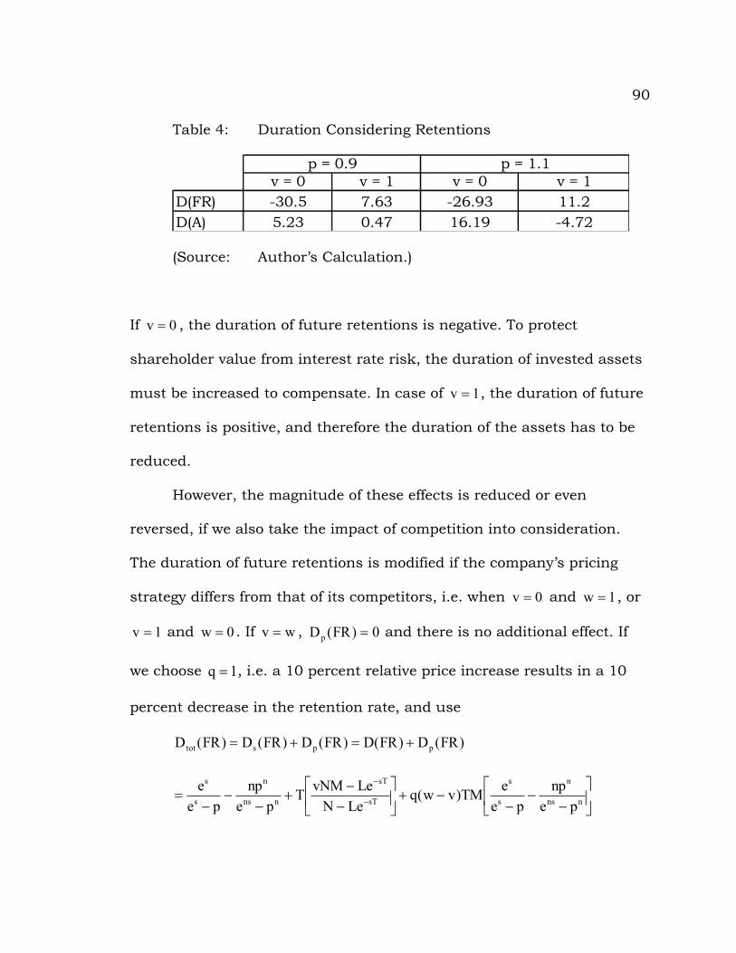
90

Table 4: Duration Considering Retentions

v = 0 v = 1 v = 0 v = 1D(FR) -30.5 7.63 -26.93 11.2D(A) 5.23 0.47 16.19 -4.72

p = 0.9 p = 1.1


If 0v = , the duration of future retentions is negative. To protect

shareholder value from interest rate risk, the duration of invested assets

must be increased to compensate. In case of 1v = , the duration of future

retentions is positive, and therefore the duration of the assets has to be

reduced.

However, the magnitude of these effects is reduced or even

reversed, if we also take the impact of competition into consideration.

The duration of future retentions is modified if the company’s pricing

strategy differs from that of its competitors, i.e. when 0v = and 1w = , or

1v = and 0w = . If wv = , 0)FR(Dp = and there is no additional effect. If

we choose 1q = , i.e. a 10 percent relative price increase results in a 10

percent decrease in the retention rate, and use

)FR(D)FR(D)FR(D)FR(D)FR(D ppstot +=+=

úû

ùêë

é-

--

-+úû

ùêë

é--

+-

--

= -

-

nns

n

s

s

sT

sT

nns

n

s

s

penp

peeTM)vw(q

LeNLevNMT

penp

pee

91

úû

ùêë

é-

--

-+úû

ùêë

é--

+-

--

= ××-

×-

× 1503.015

15

03.0

03.0

203.0

203.0

1503.015

15

03.0

03.0

pep15

pee2)vw(

e100089.993e100089.993v2

pep15

pee

we get the following results for the total duration of future retentions and

the risk-minimizing duration of the invested assets.

Table 5: Duration Considering Retentions and Competition

v = 0 and w = 1 v = 1 and w = 0 v = 0 and w = 1 v = 1 and w = 0Dp(FR) 11.26 -11.26 18.4 -18.4Dtot(FR) -19.24 -3.63 -8.53 -7.2

D(A) 3.82 2.83 -8.67 11.51

p = 0.9 p = 1.1


We can clearly see that for 0v = the total duration of future

retentions is greater than the duration of future business we obtained

just considering future business, and the duration of the assets has to be

decreased to compensate. The extent to the duration of the assets has to

be modified is determined by the present value of future retentions. For

1v = the total duration of future retentions is less than the duration of

future business in table 4, and therefore the duration of the invested

assets has to be increased. Note that for 9.0p = the duration of the assets

we obtained when future retentions and the effects of competition were

92

considered, are greater than the duration of the assets we got, when

these two factors were ignored.

93

CHAPTER V

SUMMARY

Asset-liability management gained importance in the United States

in the 1970s when interest rates increased sharply, became more volatile

than ever before, and options embedded in the assets and liabilities were

exercised more frequently. Asset-liability management primarily intended

to eliminate this interest rate risk, basically by applying Redington’s

main idea of an equal and parallel treatment in the valuation of assets

and liabilities, and his concepts of duration and immunization. The

strength and the weakness of the traditional immunization strategy

resulted in the development of all modern techniques of asset-liability

management. We can classify them into static techniques and dynamic

strategies. The static techniques focus on a complete match between

assets and liabilities. But they fail to consider the trade-off between risk

and return. The value driven dynamic strategies generally modify

Redington’s concept of immunization to protect a company’s surplus

from interest rate risk. The return driven strategies mainly focus on

94

returns earned by company. All these methods have their potential

advantages and disadvantages, and focusing on one risk might increase

other kinds of risk. Therefore, several of these methods should be used

simultaneously and an optimal trade-off between risk and return has to

be determined in order to reduce not only interest rate risk, but the

overall risk exposure of a company.

Statutory, GAP and tax accounting fail to recognize changes in the

present value of cash flows according to changes in interest rate,

embedded options in assets and liabilities, and possible future profits

generated by existing and future policies. But when conducting asset-

liability management, it is important to consider future business and see

the company as an ongoing concern. Assets and liabilities that refer to

future business not yet written have to be taken into account, because

they are real and reflected in the market value of the company. In order

to protect the shareholder value of a company, i.e. find the risk-

minimizing investment strategy, a company’s investment and pricing

strategy have to be coordinated. But the pricing strategy of the

company’s main competitors and the sensitivity of customers to price

differences between the company and its competitors also have to be

taken into account.

95

Hence, asset-liability management can be seen as an ongoing

process of formulating, checking and revising strategies associated with

assets and liabilities both from existing and future business in order to

attain a company’s financial objectives, given the company’s risk

tolerances and other constraints. Asset-liability management has to

control the interest rate risk without neglecting the asset default risk, the

product pricing risk and other uncertainties.

96

REFERENCES

Alexander, M. et al., eds. (2003). Life Insurance Fact Book 2003.

Washington D.C.: American Council of Life Insurers. Atkinson, D. B. and J. W. Dallas, (2000). Life Insurance Products and

Finance. Schaumburg, IL: Society of Actuaries. Baznik, C., M. Beach, G. Greenberg, V. Isakina, and J. Young (2003).

Professional Actuarial Specialty Guide Asset-Liability Management. Schaumburg, IL: Society of Actuaries.

Black, K. and H. D. Skipper (2000). Life & Health Insurance. Upper

Saddle River, NJ: Prentice Hall. Bodie, Z., A. Kane, and A. J. Marcus (1996). Investments. Boston, MS:

Irwin/McGraw-Hill. Cox, J. C., J.E. Ingersoll and S.A.Ross (1985). “A Theory of Term

Structure of Interest Rates,” Econometrica 53: 385-407. Dicke, A. A. (1996). Comparison of Methods for Fair-Valuing Life Insurance

Liabilities. New York, NY: Irwin. Feldblum, S. (1989). Asset Liability Matching for Property/Casualty

Insurers. Arlington, VA: Casualty Actuarial Society. Gajek, L., K. Ostaszewski, and H.-J. Zwiesler (2004). “Primer on Duration

and Convexity,” Illinois State University working paper, submitted to the Journal of Actuarial Practice.

Gardner, M. J. and D. L. Mills (1991). Managing Financial Institutions, An

Asset/Liability Approach. Chicago, IL: The Dryden Press. Hicks, J.R. (1939). Value and Capital. Oxford: Clarendon Press.

97

Ho, T. S. Y. (1990). Strategic Fixed Income Investment. Homewood, IL: Dow Jones-Irwin.

Huebner, S. S., K. Black, and R. S. Cline (1982). Property and Liability

Insurance. Englewood Cliffs, NJ: Prentice Hall. Insurance Information Institute (2004).

http://www.financialservicesfacts.org. New York, NY (cited 20. May 2004).

Laster, D. and E. Thorlacius (2000). “Asset-Liability Management for

Insurers,” in Sigma. Zuerich, Swiss: Swiss Reinsurance Company Economic Reaserach & Consulting.

Leibowitz, M. L., and A. Weinberger (1982). “Contingent Immunization-

Part I: Risk Control Procedures,” Financial Analysts Journal (November-December): 17-31.

Leibowitz, M. L., and A. Weinberger (1983). “Contingent Immunization-

Part II: Problem Areas,” Financial Analysts Journal (January-February): 35-50.

Leland, H., and M. Rubinstein (1981). “Replication Options with Position

in Stocks and Cash,” Financial Analysts Journal (July-August): 63-72.

Lintner, J. (1965). “The Valuation of Risky Assets and the Selection of

Risky Investments in Stock Portfolios and Capital Budgets,” Review of Economics and Statistics 47:13-37.

Macaulay, F. R. (1938). Some Theoretical Problems Suggested by the

Movements of Interest Rates, Bond Yields, and Stock Prices in the United States since 1856. Cambridge, MA: National Bureau of Economic Research.

Markowitz, H. (1952). “Portfolio Selection,” Journal of Finance 7: 77-91. Miller, L., U. Rajan, and P. A. Shimpi (1989). “Realized Return

Optimization: A Strategy for Targeted Total Return Investing in the Fixed Income Markets,” in The Institutional Investor Focus on

98

Investment Management, edited by Frank J. Fabozzi. Cambridge, MA: Balinger Publishing.

Mooney, S. and L. Cohen (1991). Basic Concepts of Accounting and

Taxation of Property/Casualty Insurance Companies. New York, NY: Insurance Information Institute Press.

Panjer, H. H. et al., eds. (1998). Financial Economics: With Applications to

Investments, Insurance and Pensions. Schaumburg, IL: The Actuarial Foundation.

Panning, W. H. (1987). “Asset-Liability Management: Beyond Interest

Rate Risk,” in Financial Analysis of Insurance Companies. Arlingtion, VA: Casualty Actuarial Society.

Panning, W. H. (1993). Asset-Liability Management for a Going Concern,

in Dynamics of the Insurance Industry, New York, NY: Irwin. Ostaszewski, K. (2002). Asset-Liability Integration SoA Monograph M-FI02-

1. Schaumburg, IL: Society of Actuaries. Redington, F. M. (1952). “Review of the Principles of Life Office

Evaluation,” Journal of the Institute of Actuaries 78(350, part 3): 286-340.

Reitano, R. R. (1991a). “Multivariate Duration Analysis,” Transactions of

the Society of Actuaries 43: 335-376. Reitano, R. R. (1991b). “Multivariate Immunization Theory,” Transactions

of the Society of Actuaries 43: 393-428. Ross, S. A. (1976). “The Arbitrage Theory of Capital Asset Pricing,”

Journal of Economic Theory 13: 341-360. Samuelson, P. A. (1945). “The Effect of Interest Rate Increases on the

Banking System,” American Economic Revue (March): 16-27. Shiu, E. S.W. (1993). “Asset-Liability Management: From Immunization

to Option-Pricing Theory,” in Financial Management of Life Insurance Companies. Norwell, MA: Kluwer Academic Publishers.

99

Tullis, M. A. and P. K. Polkinghorn (1996). Valuatio of Life Insurance Liabilities. Winsted, CT: Actex Publications.

Van der Meer, Robert and Meye Smink (1993). “Strategies and

Techniques for Asset-Liability Management: An Overview,” The Geneva Papers on Risk and Insurance, 18 (No. 67, April 1993): pp. 144 – 157.

Webfinance Inc. (2004). http://www.investorwords.com. Annandale, VA

(cited 15. June 2004).

asset-liability management for - illinois state...

Documents