asset and liability management: applications for the … · asset and liability management:...

MAY 2014

Asset and Liability Management: Applications for the Management and Modeling of Non-Maturing DepositsAbstract

Non-maturing deposits (NMDs) are an important source of long-term low-cost funding for a bank. This paper seeks to establish an integrated framework for the valuation, interest rate risk quantification, and funds transfer pricing of non-maturing deposits (NMD). In order to understand the impact of rates and economic variables on the various behavior factors that drive deposit behavior, a bottom-up statistical analysis of the underlying data must be performed. The entire process from data collection through cash flow generation is explicitly addressed. Furthermore, in order to understand the impact of deposit behavior on the risk management and profitability of a bank, the underlying deposit modeling assumptions for net interest income (NII) simulation, valuation, and funds transfer pricing (FTP) must be consistent. Otherwise, inconsistent and sub-optimal decision making may result. The paper concludes that NMD behavior modeling could more accurately quantify the risk of the balance sheet and can be a source of value creation and return enhancement for a financial institution.

MODELING METHODOLOGY

Authors

Robert J. Wyle, CFA

Contact UsFor further information please contact our customer service team:

Americas +1.212.553.1653 [email protected]

Europe +44.20.7772.5454 [email protected]

Asia-Pacific +85.2.3551.3077 [email protected]

Japan +81.3.5408.4100 [email protected]

WyleR

Sticky Note

Unmarked set by WyleR

2 MAY 2014 MODELING METHODOLOGY: ASSET AND LIABILITY MANAGEMENT: APPLICATIONS FOR THE MANAGEMENT AND MODELING OF NON-MATURING DEPOSITS

MOODY’S ANALYTICS

CONTENTS

1 INTRODUCTION ........................................................................................................................................ 3

2 NMD MODELING APPROACHES ............................................................................................................. 4

3 THE DATA .................................................................................................................................................... 5

3.1 Data Requirements ...............................................................................................................................5

3.2 Data Quality and Data Scrubbing .....................................................................................................5

4 MODELING DEPOSIT CASH FLOWS ....................................................................................................... 6

4.1 A simple Model for Estimating Deposit Decay ..............................................................................6

4.2 A More Complex Model for Estimating NMD Run-off .................................................................9

4.3 Estimating the Paid Rate ................................................................................................................... 11

4.4 NMD Balances and Terms .................................................................................................................12

5 NMD FUNDS TRANSFER PRICING (FTP) ...............................................................................................15

5.1 NMD Funds Transfer Pricing Methods ............................................................................................15

5.2 NMD FTP Practical Examples ...........................................................................................................17

6 RISK MANAGEMENT IMPLICATIONS OF NMD CASH FLOW MODELING ...................................... 22

6.1 Impact of NMD on Market Value Sensitivity ............................................................................... 23

6.2 Impact of NMD on FTP ..................................................................................................................... 24

7 CONCLUSION .......................................................................................................................................... 24


MOODY’S ANALYTICS

1 Introduction

Non-maturing deposits (NMDs) are a low-cost long-term source of funding and are a significant determinant of the intrinsic value of a bank. The prudent measurement and management of core deposits is an essential activity for any bank and is a source of interest rate risk mitigation, return enhancement, and value creation.

NMDs are defined as demand deposit accounts (DDAs), negotiable order of withdrawal (NOW) accounts, money market deposit accounts (MMDAs), and passbook accounts. As the name would imply, non-maturing deposits arise from the fact that these funds, unlike other forms of bank funding, such as certificates of deposit (CDs), carry no explicit maturity date. Rather, the depositor possesses a long deposit redemption option while the bank is short an embedded option. This lack of a contractual maturity is often called behavior because the retention of core deposits is driven by how retail consumers perceive the value that they obtain relative to alternative uses for their funds. Statistical behavior models that isolate the risk factors that drive consumer preferences are typically used to understand deposit cash flows, profitability, and value.

The primary determinants of deposit cash flows are retention and the rate sensitivity of the offered rate. Deposit balance retention refers to the decay of deposits in existing accounts over time. The degree of correlation (pricing coefficient) between the rate paid to the customer (offered rate) on the account and short-term interest rates defines the sensitivity of the offered rate. An intuitive understanding of the relationship between the paid rate and the rate of deposit decay can be illustrated with the image of water flowing from a tap into and out of a basin.

The rate at which the water flows out of the basin is a function of both tangible and intangible value received in terms of the offered rate paid, product services, and other perceived value. If the retail deposit unit increases the paid rate beyond what existing customers demand, then the water level in the basin rises. This practice is commonly known as buying “hot money” and tends to undermine the value of the deposit franchise because it is likely to attract undesirable clients who withdraw money when market rates rise. Conversely, water flows out of the basin more quickly and the waterline falls if the paid rate is not increased sufficiently in response to changes in market rates or service deteriorates. Finally, the balance of core deposits remains stable as long as the rate at which water flows out of the tap is the same as how fast water flows out of the basin. This state is considered equilibrium.

The simple analogy of controlling the water level by regulating the flow of water pouring in and out of the basin illustrates the problem of managing the deposit base at a reasonable cost. The quantitative tools and governance required to manage core deposits are the topic of this white paper.

A common model known as the vintage run-off model helps to illustrate the behavior, risk management, and performance measurement of core deposits.


MOODY’S ANALYTICS

2 NMD Modeling Approaches

There are many different approaches for modeling NMDs. While they may be different structurally, they all seek to achieve the same goals. Therefore, it is important to bear in mind some of the key challenges when designing a deposit model:

» How long does it take for existing deposits to run-off?

» How do I determine repricing assumptions and separate them from maturity assumptions (rate risk versus term risk)?

» How to segment portfolios to capture the key behavior characteristics defining cash flow?

» How do I measure profitability?

Some of the NMD modeling techniques currently used by banks, and which also appear in the academic literature include the following:

» Hutchinson and Pennacchi (1996)

» Jarrow and Van Deventer (1998):

» Schurle (1998) O’Brien (2000)

» Replicating Model (Antoine Frachot, 2003)

» Kalkbrener and Willing (2004)

» Elkenbracht and Nauta (2006)

The deposit models listed in the preceding section can either be categorized as theoretical models or empirical models. Theoretical approaches tend to vary seeking to explain NMD behavior using arbitrage free stochastic simulation, contingent claims models, equilibrium approaches, or options as proxies. Empirical models are fundamentally different seeking to explain NMD behavior with various forms of time series analysis on the historical deposit data. Unsurprisingly each deposit modeling technique has strengths and weaknesses. Banks must evaluate which model to choose, based on their goals, resources, modeling capability, and institution-specific depositor behavior characteristics.

Rather than evaluate each of these modeling approaches, a form of empirical model known as the vintage run-off model illustrates NMD behavior and its impact on the risk of a bank. The vintage run-off model seeks to segregate deposit balances based on historical tranches called vintages. A vintage consists of all of the individual accounts for a non-maturing deposit account type that are opened within a particular month. Cash flow behavior characteristics are applied to each vintage by calculating the monthly decay within each vintage. Therefore, the vintage account run-off model characterizes the manner in which accounts close over time. Applying a forecast of the paid rate to the NMD deposit balances net of account run-off provides both nominal and interest cash flows needed for both income forecasting and valuation.

NMD balances are sometimes broken down first by product, and within product, by tier. This approach better isolates and models consumer preferences. Some banks further segment products within product tier demographically. For example, older depositors may have different needs relative to younger ones. More granular analysis helps to identify the drivers of key behavior characteristics in order to model cash flows.


MOODY’S ANALYTICS

3 The Data

Clean deposit data is notoriously hard to gather. Unsurprisingly, the adage “garbage-in, garbage-out” has particular meaning for purposes of deposit modeling. Some of the chronic deposit data problems include acquisitions, changes to deposit product features, and the shortcomings of outdated legacy core banking systems. All of these factors contribute to the difficulties encountered when seeking clean deposit data over the term of at least one business cycle. The following commentary is intended to set some general guidelines in terms of deposit data requirements, quality, and data cleansing issues.

3.1 Data Requirements

Ideally, the minimum data requirement needed for a valid deposit study is at least one business cycle to capture the joint behavior of funds savers/lenders and funds consumers/gatherers. In the past, two years of monthly deposit data were sufficient. At a minimum, the following data is required:

» Product type, such as checking or savings

» Product tier within product type

» Origination date

» Date of account closure

» Ending balance

» Average balance

» Paid Rate

Given the data problems that are normally encountered, it is important to understand the data. Specifically, what process did the bank follow to cleanse the historical deposit data and to deal with missing data or outliers? For instance, in the case of fraud where client accounts were compromised and new account numbers issued, was the time series adjusted to reflect whether the account is seasoned and old? Alternatively, if the account was converted from one product to another, was the data adjusted?

3.2 Data Quality and Data Scrubbing

Common data idiosyncrasies and corresponding filters and/or transformations intended to scrub the data of bias include:

» Retain accounts that have non-zero average and/or ending balances for purposes of deposit modeling. That is, exclude any account that maintained a zero balance during the deposit study time horizon and was never funded from the analysis.

» Accounts may be active, but may not have balances. Therefore, assume accounts are “open” on the first date that a given account has a positive balance.

» Deposit accounts may remain active even though they have zero balances. Therefore, assume that accounts are closed when the account balance goes to zero and remains at zero.

» Remove any account from a deposit study that has multiple account opening dates.

» Retail deposits from different banks may be combined due to mergers and acquisitions. However, the acquired deposits may not be consistent with the legacy history or may be assigned a new origination date. If there are acquired deposits during the deposit study time period, it may be necessary to remove these accounts in order to avoid biasing the data.


MOODY’S ANALYTICS

» There could be circumstances under which individual accounts can shift between responsibility centers. Therefore, an account may have been considered Retail at one point and then Commercial at other points in time. Exclude these accounts from a deposit study to more clearly delineate retail versus commercial behaviors throughout a deposit study.

» Surge balances are a form of deposit behavior where balances flow into retail accounts in response to some systemic event and then suddenly flow out after the effect of the systemic event reverses. For example, after the attack on the World Trade Center on September 11, 2001, investors withdrew their funds from the equity markets and placed them in bank accounts. Approximately 18 months later, investors reverted to their long-term behavior and withdrew these funds from their bank accounts and reinvested them in the equity markets. Remove surge balances from the data for purposes of deposit modeling and account for them separately.

4 Modeling Deposit Cash flows

In order to calculate the market value, duration, or transfer price of an NMD account, the cash flows that the account generates must be modeled. The market value for NMDs is the present value of the cash flows discounted at the LIBOR curve (or some other risk free rate). For purposes of NMD cash flow modeling, the two critical assumptions are:

» Deposit balance retention refers to the decay of deposits in existing accounts over time.

» The degree of correlation (pricing coefficient) between the rate paid to the customer (offered rate) on the account and short-term interest rates.

The balance retention (balance decay) assumption is required to model principal cash flows while the correlation of the offered rate to market rates is required to model interest cash flows. The discounted cash flow of both principal and interest define the market value. The sensitivity of market value to changes in rates is the concept of duration (see “An Evaluation of Interest Rate Risk Tools and the Future of Asset Liability Management”; Robert J. Wyle; March 2013).

4.1 A simple Model for Estimating Deposit Decay

Deposit retention is defined as the percentage of balances retained from a certain point in time forward for a constant set of accounts. Conversely, decay is the percentage of balances that run-off. Balances are assumed to undergo a natural decay as existing accounts run-off over time. Therefore, deposit decay may be represented by the following equation:

Figure 4.1 together with equation 4.1 illustrate the calculation of deposit decay from January 31, 20xx through February 28, 20xx.

Equation 4.1

Where,

SMM/Decayt = The single monthly mortality or deposit decay from time January 20xx to February 20xx Balt = The average deposit balance per vintage in February 20xx Balt-1 = The average deposit balance per vintage in February 20xx Average SMM = The average SMM for all vintages from January 20xx to February 20xx

Conversely, equation 4.2 illustrates the calculation of deposit retention:


MOODY’S ANALYTICS

Equation 4.2

Figure 4.1

Jan 31, 20xx Feb 28, 20xx

Vintage Vintage Vintage Vintage

Age Balance Age Balance SMM

0

0 $1,965.24 1 $1,914.88 2.56%

1 $1,162.05 2 $1,132.87 2.51%

2 $1,575.71 3 $1,535.22 2.57%

3 $1,715.09 4 $1,672.96 2.46%

4 $1,653.69 5 $1,611.00 2.58%

5 $1,208.11 6 $1,177.72 2.52%

. .

. .

. .

30 $669.30 31 $653.14 2.41%

31 $740.74 32 $722.28 2.49%

32 $751.75 33 $733.44 2.44%

Average SMM 2.50%

The example in Figure 4.1 represents a single calculation for decay from two “snap shots” in time – January 20xx and February 20xx. In reality, a longer time series of deposit portfolio snap shots is needed – at least two years. Therefore, a deposit decay curve is really a cross sectional multi-period analysis (see figure 4.2).

Figure 4.2

Time

0 1 2 3 4 5 6 7 8 Total

Vintage 1 Avg SMM1

2 1 Avg SMM2

3 2 1 Avg SMM3

4 3 2 1 Avg SMM4

5 4 3 2 1 Avg SMM5

6 5 4 3 2 1 Avg SMM6

7 6 5 4 3 2 1 Avg SMM7

8 7 6 5 4 3 2 1 Avg SMM8

9 8 7 6 5 4 3 2 1 Avg SMM9

10 9 8 7 6 5 4 3 2 Avg SMM10

11 10 9 8 7 6 5 4 3 Avg SMM11

12 11 10 9 8 7 6 5 4 Avg SMM12

13 12 11 10 9 8 7 6 5 Avg SMM13

Average Decay Avg SMMn


MOODY’S ANALYTICS

In the example above the average decay was calculated from average balances. If the data is not clean, an alternative method is to calculate deposit decay from the number of accounts per vintage. This approach will capture the run-off of accounts over time, and is a viable alternative as poor data can contribute to bad results. In addition, the decay curve can be constructed using a least squares method from the individual decay curves for each vintage. The advantage of this method is that it is more prospective whereas the average decay method is retrospective as it places greater emphasis on events that happened in the past.

After the SMM decay assumption is known, the deposit decay curve can be constructed. The definition of the deposit decay curve is how a one dollar deposit will run off over time. Either a constant SMM or piece-wise linear interpolation can be used to construct the curve. Figure 4.3 illustrates both constant SMM and piece-wise interpolation using the simple example in Figure 4.1:

Figure 4.3

Exponetial Model Piece-wise linear model

Start End % of Original

Constant SMM Period Period Balance

5.00% 0 3 4.75%

3 7 3.98%

7 10 3.32%

Period Balance Balance

0 $100.00 $100.00

1 $95.00 $95.25

2 $90.25 $90.49

3 $85.74 $85.74

4 $81.45 $81.76

5 $77.38 $77.79

6 $73.51 $73.81

7 $69.83 $69.83

8 $66.34 $66.51

9 $63.02 $63.19

10 $59.87 $59.87

$55.00

$60.00

$65.00

$70.00

$75.00

$80.00

$85.00

$90.00

$95.00

$100.00

$105.00

0 1 2 3 4 5 6 7 8 9 10

Exponential Piece-Wise Linear


MOODY’S ANALYTICS

Both the decay curve created with a constant SMM or with piece-wise linear interpolation are extremely close. The decay curve is an exponential function. Just as human behavior can be described with a normal distribution, deposit run-off can be described with an exponential decay function.

4.2 A More Complex Model for Estimating NMD Run-off

Deposit models should explicitly account for behavior. As discussed earlier, there are many ways to model behavior. Financial institutions must determine the best method for their deposit portfolio and macro-economic drivers. For purposes of this analysis, we take up where we left off in figure 4.2 and apply the vintage run-off model to illustrate the impact of deposit risk factors on deposit cash flows. The underlying vintage balance run-off model consists of a vintage account run-off model combined with an individual account average balance model.

Some of the most common NMD behavior risk factors include:

» The sensitivity of average balances in response to changes in the level, direction, and magnitude of interest rates

» Seasonality, such as seasonal variation in the level of core deposits

» The impact of vintage age on run-off

» The cannibalization of NMD balance in response to term deposit pricing

Savings, DDA, and NOW accounts usually display seasonal variations but lack interest rate sensitivity. However, MMDAs are typically sensitive to changes in interest rates. This difference in behavior is because DDA and NOW depositors generally seek the convenience of facilitating monetary transactions, whereas depositors in MMDAs are more interested in return. Typically, deposit model parameters are calibrated for each product sub-type, using multiple linear regression based on historical month average account balance data.

4.2.1 The Vintage Account Run-off Model

The vintage account run-off model characterizes the manner in which the accounts that make up a vintage close over time. The form of the model in this example assumes that a vintage’s accounts are divided into two pools: A fast run-off pool and a slow run-off pool. Assume that the fraction of each new vintage that initially falls into each pool is constant over time, from vintage to vintage. For each pool, a constant percentage of the remaining accounts close during each subsequent time period (months) resulting in an exponential decay in the number of open accounts for each pool. Exponential functions are frequently used to model both growth and decay. In this illustration, the equation form of the model is:

Equation 4.3

Where,

λ N(t) Number of open accounts in the vintage at the end of month t. N(0) Initial total number of accounts in the vintage. F Fraction of new vintage accounts in the fast run-off pool. S Fraction of new vintage accounts in the slow run-off pool. λf Fast run-off account pool decay constant. λs Slow run-off account pool decay constant.


MOODY’S ANALYTICS

Monthly vintage data snap shots for the number of accounts opened at month-end, the number of accounts closed at month-end, and the end-of-month balance by vintage and sub-product are required to parameterize equation 4.3. The account run-off parameters are determined for each NMD product sub-type by selecting values for F, S, λf, and λs that minimizes the sum of the squared error between the model and the associated account vintage run-off data sets.

4.2.2 The Vintage Account Average Balance Model

An average balance model is needed for multiple reasons.

First, for funds transfer pricing, a bank typically does not have snap shot vintage data going back to the creation of each account. Therefore, the original vintage balances must be reconstructed starting from the initial reporting date when the deposit portfolio is first transfer priced. Also, the balance model is needed when deposit modeling assumptions are changed, and the deposit portfolio must be re-transfer priced. Retail is not rewarded when they lengthen the average life of deposits or penalized when the average life shortens unless these cash flow changes are reflected in the transfer pricing results. Otherwise, if retail receives the same transfer rate regardless of performance, then service may suffer.

Second, a balance projection is needed for the fixed core, the floating core, and the volatile balance (see “Terms and Balances”; Section 4.4) for purposes of NII forecasting, liquidity risk management, and market value at view date. Since the components affect the repricing characteristics, transfer pricing results and duration of deposits, the total balance and the components must make sense both prospectively and relative to the others. Therefore, a statistical model is needed for each component rather than a simple moving average used to obtain the fixed/floating core split which is more retrospective in nature.

Third, a balance model is needed for purposes of stress testing. In particular, the Comprehensive Capital Analysis and Review (CCAR) exercise is forcing banks to develop models that incorporate the impact of macro-economic variables. Empirically, there is strong economic and statistical evidence indicating that macro-economic variables matter when constructing stress testing assumptions. Macro-economic exogenous variables influence retail consumer and institutional behavior. Recent models take an econometric approach that links deposit growth to CCAR and other macro-economic variables or their lags. Both statistical models and economic intuition can be used to guide the selection of explanatory variables in a regression. Projected values of CCAR and other macro-economic variables are fed to the estimated regression equations to project deposit growth rates and balances under various stressed scenarios.

The vintage pool average balance model used for purposes of this discussion has a simple slope intercept form . The intercept value represents the average initial balance of the accounts in each run-off pool when the vintage is new. The slope values represent the constant amount by which the average balances of the remaining open accounts in each run-off pool increase or decrease each month. The slope intercept values can be calculated by linear regression using the vintage balance data in the monthly snap shot data sets and the parameterized account run-off models.


MOODY’S ANALYTICS

The deposit average balance equations are intended to provide accurate estimates of future month average balances for the various NMD accounts. The form of such a model might look like the following:

Equation 4.4

Where,

Bal(t) = The total average account balance in month t. ∆Bal(t) = Change in total average account balance from month t-1 to month t. r(t) = The reference interest rate level at the end of month t. ∆CDU(t) = Change in total CDs < $100k account balance from month t-1 to month t. SFact(t) = The seasonal factor that applies for month t. Ci = Model parameterization constants.

The model is parameterized for each sub-product by determining the values of the seasonal factors (SFact(t)) and the model parameterization constants (Ci) that cause the model to best reproduce the historical values of Bal(t) given the historical values of ∆Bal(t), r(t), and ∆CDU(t). The best fit can be determined by first calculating the seasonal factors if appropriate and then using multiple linear regression to determine the best Ci values from de-seasonalized historical data.

4.3 Estimating the Paid Rate

The paid rate function is normally a multiple linear regression and seeks to forecast the level of deposit rates into the future, based on movements in short-term market rates. Therefore, the paid rate function represents the correlation between the offered rate and short-term benchmarks.

Typical historical data issues which make it difficult to estimate the paid rate include low rates or an arbitrary pricing strategy. If short-term rates move to a low absolute level for an extended period, then the paid rates may be priced at an implicit rate floor. Therefore, it has exhibited no co-movement with rates. If this floor data is used in the estimation data set, the result is low interest sensitivity and a high effective duration. Second, a bank’s pricing strategy may be arbitrary. For example, if the pricing strategy is to offer a paid rate that is within the high and the low for the six largest regional competitors, then finding a meaningful correlation may be difficult.

The easiest way to determine pricing policy is to negotiate the pricing coefficients with the retail business unit. There can be a negotiated rate coefficient in the up state and a different rate in the down state. However, useful market data may be lost for lack of performing time series analysis which can provide insight into what compensation the depositors in each sub-type require when market rates change. Second, a simple linear regression may be constructed of the form:

Equation 4.5

Where,

β = The rate pricing coefficient passed through to the depositor given changes in short-term market rates Rt = The short-term market rate benchmark at time period t. R(t-n) = The short-term market rate benchmark at time period t – n.


MOODY’S ANALYTICS

Alternatively, the paid rate function can be a complex multiple linear regression based on multiple market rates and macro-economic variables and their lags as well as depending on the specific circumstances of the bank.

4.4 NMD Balances and Terms

So far we have considered the problem of how to characterize the manner in which deposits run-off, how to predict deposit balances in the future, and how to price the NMD paid rate. Additional problems that must be considered are:

» How to segment portfolios in order to differentiate between core balances that can and cannot be statistically predicted?

» How to determine repricing assumptions and separate them from maturity assumptions, if possible (rate risk versus term risk)?

» How to establish the term of an NMD account given that the run-off function is defined as an exponential decay function?

These questions are typically answered by statistical analysis of the empirical data which sheds light on which balances are persistent versus balances that are not persistent, and how managed rate products reset. In performing these analyses, firms must make assumptions for when to re-strip historical vintages.

NMDs are typically broken down into a core balance and a volatile balance. The core balance is that portion of a deposit that is statistically predictable from month-to-month and represents a long-term source of funding. The volatile balance is that portion of the account balance that is not statistically predictable. Therefore, it is given a shorter maturity from one day to one month and has a lower transfer price. There are a number of ways to determine the core/volatile split.

1. Use the Moving Average

The easiest way to quantify the core/volatile split is to use a moving average. For example, a bank can make the assumption that the core is based on a six month moving average of the historical total balance. A bank can even use multiple look back periods such as 60% of the six-month moving average and 40% of the three-month moving average. The moving average is the core and the difference between the total balance and the moving average is the volatile balance. However, a moving average is not a statistical model and the definition of the lookup period is at best subjective. Therefore, this method is not recommended.

2. Use the Properties of a Normal Distribution

A second and statistically more viable method to define the core/volatile split is to use the properties of a normal distribution. A normal distribution can be estimated by calculating the mean and standard deviation of the monthly instrument-level historical average balances. All that is needed is an estimate of the mean and standard deviation. For example, using a 5% alpha one can estimate that next month there is a 95% probability that the average balance per account will be greater than the 95% lower bound.


MOODY’S ANALYTICS

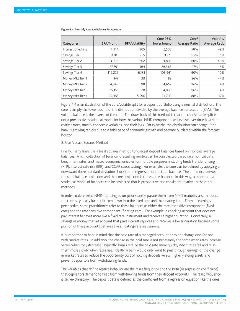
Figure 4.4: Monthly Average Balance Per Account

Categories BPA/Month BPA VolatilityCore 95%

lower boundCore/

Average RatioVolatile/

Average Ratio

Interest Checking 4,314 905 2,503 58% 42%

Savings Tier 1 9,781 255 9,271 95% 5%

Savings Tier 2 3,008 602 1,805 60% 40%

Savings Tier 3 27,291 464 26,363 97% 3%

Savings Tier 4 119,222 6,131 106,961 90% 10%

Money Mkt Tier 1 147 33 82 56% 44%

Money Mkt Tier 2 4,848 98 4,652 96% 4%

Money Mkt Tier 3 25,155 528 24,099 96% 4%

Money Mkt Tier 4 95,985 5,596 84,792 88% 12%

Figure 4.4 is an illustration of the core/volatile split for a deposit portfolio using a normal distribution. The core is simply the lower bound of the distribution divided by the average balance per account (BPA). The volatile balance is the inverse of the core. The draw-back of this method is that the core/volatile split is not a prospective statistical model for how the various NMD components will evolve over time based on market rates, macro-economic variables, and their lags. For example, the distribution can change if the bank is growing rapidly due to a brisk pace of economic growth and become outdated within the forecast horizon.

3. Use A Least Squares Method

Finally, many firms use a least squares method to forecast deposit balances based on monthly average balances. A rich collection of balance forecasting models can be constructed based on empirical data, benchmark rates, and macro-economic variables for multiple purposes including funds transfer pricing (FTP), interest rate risk (IRR), and CCAR stress testing. For example, the core can be defined by applying a downward three standard deviation shock to the regression of the total balance. The difference between the total balance projection and the core projection is the volatile balance. In this way, a more robust statistical model of balances can be projected that is prospective and consistent relative to the other methods.

In order to determine NMD repricing assumptions and separate them from NMD maturity assumptions, the core is typically further broken down into the fixed core and the floating core. From an earnings perspective, some practitioners refer to these balances as either the rate insensitive component (fixed core) and the rate sensitive component (floating core). For example, a checking account that does not pay interest behaves more like a fixed rate instrument and receives a higher duration. Conversely, a savings or money market account that pays interest reprices and receives a lower duration because some portion of these accounts behaves like a floating-rate instrument.

It is important to bear in mind that the paid rate of a managed account does not change one-for-one with market rates. In addition, the change in the paid rate is not necessarily the same when rates increase versus when they decrease. Typically, banks reduce the paid rate more quickly when rates fall and raise them more slowly when rates rise. Ideally, a bank would only want to pass through enough of the change in market rates to reduce the opportunity cost of holding deposits versus higher yielding assets and prevent depositors from withdrawing funds.

The variables that define reprice behavior are the reset frequency and the Beta (or regression coefficient) that depositors demand to keep from withdrawing funds from their deposit accounts. The reset frequency is self-explanatory. The deposit beta is defined as the coefficient from a regression equation like the ones


MOODY’S ANALYTICS

described in section 4.3 and documented in equation 4.5. The interpretation of the deposit beta is the portion of the paid rate that is either increased or decreased for every hundred basis point movement in market rates. Therefore, a deposit beta of 0.7 is interpreted as a 70-bps increase in the paid rate for every 100-bps increase in the relevant market rate benchmark.

There are several ways to determine the fixed/floating core split. First, the split can be negotiated. If the transfer pricing manager has a view of past or target repricing behavior of depositors, the reset frequency and the fix/floating core split can be negotiated with the retail business unit. Second, the beta from a least squares method can be used to define the split. Regardless of the method chosen, if the retail business unit resets the managed rate more frequently than agreed, or increases the rate beyond what depositors require, then the economic incentives implied by the assumptions of the funds transfer pricing framework influence the Retail business units pricing strategies.

Finally, assumptions for the various NMD terms must be determined. These decisions are a critical factor since they affect everything from Market value to FTP to the effective duration of deposits. There are three basic terms that must be quantified:

1. The truncation term

2. The reprice term

3. The weighted average life

The truncation term is also known as the liquidity term or the re-strip term. Since the run-off profile for the vintage run-off model is an exponential decay function, it is customary to truncate the cash flows and re-strip the remaining balances. There is no need for a truncation term in the replicating model used predominantly in continental Europe and Asia because it assumes a five-year linear run-off and is therefore not an exponential function. The reason for truncating the remaining cash flows for the vintage run-off model is that otherwise the cash flows are unrealistically long and the market and duration will be distorted. Therefore, the main consideration is the assumption for the truncation term.

The truncation term has to align with the maturity distribution for assets, consistent with the asset/liability matching principle. There are a number of ways to explain this concept. The most direct explanation is that the truncation term must be consistent with the overall maturity of the asset side of the balance sheet. Otherwise, the duration of equity will be artificially low if the duration of liabilities is too high ( see “An Evaluation of Interest Rate Risk Tools and the Future of Asset Liability Management”; Robert J. Wyle; March 2013). A more theoretical explanation is to assume that there is only one bank in the world. In such a world every loan has a corresponding deposit and every loan repayment has a corresponding inflow. Therefore, in some sense the truncation term is a means to reconcile the asset/liability matching problem. The United Kingdom typically uses a five-year truncation term, the replicating model assumes a five-year linear decay as a means of matching the repricing of assets. The United States, by contrast, generally assumes a seven- to ten-year truncation term depending on the bank or the regulator.

The reprice assumption corresponds to the reset frequency for the floating core. It directly impacts the frequency with which the funds transfer credit for interest bearing accounts is repriced. It is important because it impacts both the business unit transfer price, the NMD market value sensitivity, and NMD interest expense.

Finally, the weighted average life is the term corresponding to the observed liquidity premium. Any transfer pricing system must incent the retail deposit units to maximize not only their profitability but the weighted average life for deposits. There is no contradiction between these two goals. The term liquidity


MOODY’S ANALYTICS

premium is really the value that the liability gatherer contributes to shareholder value both from an earnings and an economic value perspective.

Both the NMD balance and term assumptions are critical inputs to the NMD modeling process. As such, they have a profound impact on a bank’s risk profile, risk management strategies, and NMD product pricing decisions. Therefore, these assumptions can either be a source of revenue enhancement or a drag on profitability.

5 NMD Funds Transfer Pricing (FTP)

Both FTP and ALM risk metrics are extensions of the basic NMD cash flows that were explored in Section 4. In fact, as we see in this section and the next, FTP is the link between market value and an accrual-based income statement. Therefore, in order to link the three legs of this stool together, modeling assumptions must be consistent.

FTP is the process through which banks allocate earnings to the various lines of business in which they are engaged (see “Implementing High Value Funds Transfer Pricing Systems”; Wyle and Tsaig; September 2011). As a critical component of a bank’s profitability measurement process, FTP allocates net interest income to various products or business units. FTP allows banks to:

» Measure business unit profitability separately from interest rate risk

» Centralize the measurement and management of interest rate risk

» Provide consistent product pricing guidance to business lines

» Set profitability targets for business units

Most banking institutions utilize funds transfer pricing in different forms and to varying degrees of complexity, and FTP for NMD is no exception. A wide range of practical application and sophistication exists across the banking industry. After the various components of NMD cash flows have been modeled, applying the relevant transfer pricing method is relatively simple. However, the specific FTP methods chosen can greatly influence the financial performance and risk management decisions made by banks. Therefore, understanding the implications of the various modeling techniques and choosing the appropriate transfer pricing approach can be complicated, as well as highly political and contentious.

5.1 NMD Funds Transfer Pricing Methods

In practice, only a few transfer pricing methodologies are routinely used, depending upon a firm’s resources and strategic goals. Methods include pooled approaches and matched-maturity funds transfer pricing. Under each method, a transfer rate is assigned to the funds provided or leant.

5.1.1 Pooled Funds Transfer Pricing Approaches

Under pooled approaches, the line of business (LOB) assigns funds to one or more pools based on pre-defined criteria and a specific set of dimensions. For instance, criteria for pool classification may be based on instrument type, term, repricing term, origination, or other fund attributes.

» The single-pool approach is the simplest method. It uses one rate to credit and charge liability and asset gatherers. The obvious advantages of the single-pool approach are that it is easy to implement and easy to understand. However, it assumes that all funds have equal importance without consideration of maturity or embedded optionality. The single-pool approach does not differentiate based on the funds’ attributes, provided or used, nor upon market conditions at the time of transaction origination. Therefore, some business units, products, or customers have an unfair advantage, while others have an unfair disadvantage. The assigned transfer rate is derived either internally, based on actual rates earned or paid, or alternatively, by market-derived interest rates.


MOODY’S ANALYTICS

» The multiple-pool approach classifies assets and liabilities into pools based on criteria such as maturity, embedded optionality, seasoning, or credit. Each pool’s assigned transfer rate is based on the unique pool criteria. For example, long maturity pools receive a long-term rate while short-term pools receive a shorter term transfer rate.

Either prevailing market rates or historical market rates are used for transfer rate assignments. When using prevailing rates, all pools are transfer-priced for each reporting period using the latest market data time series. Under the historical variation, each pool is transfer-priced using the yield curve prevailing at the time of origination. After they are assigned, transfer rates do not change over the life of the pool unless an event changes the funds’ characteristics. Multiple-pool approaches employing prevailing market rates lack the ability to measure the performance of management decisions made in the past. In contrast, using historical market rates allows for the evaluation of pricing decisions for transactions originated in prior periods. Benchmarking LOB decisions to the historical context in which those decisions were made is the preferred method.

5.1.2 Matched-Maturity Transfer Pricing Method

Matched-maturity FTP is a more detailed extension of the multiple-pool, historical variation. It is generally the preferred FTP method because it addresses the unique characteristics of funds at the cash flow level. Under this method, each source is assigned a unique and maturity-specific transfer rate, and the use of funds is based on the expected cash flow stream and the prevailing level of interest rates at the time of origination. Expected cash flows are calculated from transaction level contractual features stored in the bank’s systems of record. Behavioral assumptions are applied based on common practice and current experience for amortization, prepayment options, the short redemption option on NMD, and other embedded features. The following are the most common transfer pricing methods:

» Strip Funding: The strip funding method is defined as the transfer spread that equates the price of an instrument with the present value of its cash flows discounted against its funding curve. Therefore, the transfer spread, in this context, is defined as the economic profit in basis points above the cost of funding. The transfer spread is used to calculate the transfer rate. The transfer rate is the compensation Treasury receives for funding the loan. Therefore, the transfer rate is simply the coupon less the excess profit/transfer spread. The transfer spread never changes after it is assigned, unless there is a change in contractual features, even for floating-rate instruments. The algebraic definition of the strip funding method is:

Equation 5.1

∑ +

−+= i

n

iiii

RParSpreadRateCF

)1(*)(100

» Where, CFi = Cash flow at time period i Ratei = Instrument coupon at time period i Spreadi = Transfer spread at time period i Pari = Par value at time period i Rn = Rate from funding curve at i = n To calculate the transfer spread, solve for the spread that equates the present value of the cash flows discounted at the funding curve with the price of the instrument. The transfer rate is the instrument yield minus the transfer spread.


MOODY’S ANALYTICS

» Rate Index Method: The rate index method is used when there is no need for risk transfer. An example of a balance category where no risk transfer is needed is the trading book because these assets are typically held for a short period, for example 30 days. The transfer rate is typically a spot rate or a 30- to 90-day moving average.

» Weighted Average Life (WAL) Method: The WAL method assigns the point along the funding curve that corresponds to the WAL of the instrument being transfer priced.

» Average Rate Method: The average rate method assigns the arithmetic average of the transfer prices for each cash flow for deposits. Both time/balance weighted average rates (see equation 5.2) and weighted rates based solely on balance (see equation 5.3) are common.

Equation 5.2

Where: CFi: principal amount of cash flow i on date i (payment date of cash flow) Ti: Time between FTP_date and payment date of cash flow i, expressed in days. Ratei: Equal to getRate(Funding Curve, FTP_date, date i)

Equation 5.3

Where, CFi: principal amount of cash flow i on date i (payment date of cash flow) Ratei: equal to getRate(Funding Curve, FTP_date, date i) ∑CFi: Amount of outstanding principal at FTP date

» Maturity Method: The maturity method assigns the point along the funding curve that corresponds to the maturity term of the instrument being transfer-priced.

» Duration Method: The duration method assigns the rate along the funding curve that corresponds to the duration of the instrument being transfer-priced.

The preceding list is not complete. There are many more methods that are used throughout the globe.

5.2 NMD FTP Practical Examples

Estimating cash flows and calculating the transfer price for the various NMD components are the critical steps in the NMD performance measurement process. However, it is also important to understand how the various choices and assumptions affect the results and, in turn, how that affects deposit pricing and risk management decisions. In the next section, the vintage run-off model is used to illustrate a typical FTP reporting process. Then an example of the replicating model is used to contrast how these two approaches differ.


MOODY’S ANALYTICS

5.2.1 Vintage Run-Off Model

Monthly NMD FTP reporting is typically composed of two to three components. All non-maturity deposit products have a volatile component, and at least one of the core components. In the example below, the strip funding method is used to calculate the transfer price of each component. The following is an example using three components:

» Volatile balance FTP component = Volatile balance fraction* Over-night rate (Fed Funds Target)

» Fixed-core FTP component = Fixed-core balance fraction * Fix-core FTP rate

Figure 5.1

Business DDA

Vintage Date Vintage Age Vintage Balance Vintage FTP Rate Weighted Contribution

Jan-92 120 mo. $12,559,070 * 6.759% = 848,868

Feb-92 119 mo. $9,677,942 * 6.713% = 649,680

Mar-92 118 mo. $17,362,906 * 6.107% = 1,060,353

Apr-92 117 mo. $16,821,151 * 6.026% = 1,013,643

. . . . .

. . . . .

Sep-01 4 mo. $55,733,943 * 5.079% = 2,830,727

Oct-01 3 mo. $97,694,409 * 4.686% = 4,577,960

Nov-01 2 mo. $98,597,449 * 4.722% = 4,655,772

Dec-01 1 mo. $91,699,526 * 5.031% = 4,613,403

+ $4,220,116,540 + 268,779,222

Fixed-Core FTP Rate: 268,779,222 / $4,220,116,540 = 6.369%

Floating-core FTP component = Floating-core balance fraction* Floating-core FTP rate.

Figure 5.2

Business DDA

Vintage Date Vintage Age Vintage Balance Vintage Liquidity Prem. Weighted Contribution

Jan-92 120 mo. $12,559,070 * 2.292% = 287,892

Feb-92 119 mo. $9,677,942 * 2.568% = 248,559

Mar-92 118 mo. $17,362,906 * 2.275% = 395,006

Apr-92 117 mo. $16,821,151 * 2.503% = 420,983

. . . . .

. . . . .

Sep-01 4 mo. $55,733,943 * 2.919% = 1,626,707

Oct-01 3 mo. $97,694,409 * 2.942% = 2,873,681

Nov-01 2 mo. $98,597,449 * 2.959% = 2,917,696

Dec-01 1 mo. $91,699,526 * 2.871% = 2,633,060

+ $4,220,116,540 + 111,790,887

Floating-Core FTP Rate: 111,790,887 / $4,220,116,540 = 2.649%


MOODY’S ANALYTICS

The monthly FTP rate is the weighted average of the various NMD components:

Figure 5.3

Business DDA December 2001

Balances Balance Fractions

Volatile Balance $855,818,200 Volatile Balance Fraction 13.94%

Fixed-core Balance $4,226,899,040 Fixed-core Balance Fraction 68.85%

Floating-core Balance $1,056,724,760 Floating-core Balance Fraction 17.21%

Total Balance $6,139,442,000 (20% of total core balance)

Rates FTP Components

Over-night rate 1.930% Volatile FTP Component 0.269%

Fixed-core FTP rate 6.369% Fixed-core FTP Component 4.385%

Floating-core FTP rate 2.649% Floating-core FTP Component 0.456%

Monthly FTP rate 5.110%

5.2.2 The Replicating Model

There are both similarities and differences between the replicating model and the vintage run-off model. In both methods, the core/volatile split, the fixed core/floating core split, and the manner in which the transfer price is calculated differ.

The replicating model is complex. Therefore, only a subset of the assumptions are examined here to highlight the differences between the two approaches and understand the risk management implications. For purposes of this discussion only the decay assumption and the FTP methodology are compared.

The replicating model is a particular type of vintage run-off model that evaluates the nature of the funds by stripping the balances into portfolios of zero coupon bonds called layers. Typically, a five-year linear decay is used consistent with the assumed repricing term for total assets.

Figure 5.4

NMD Replicating Portfolio

Laye

rs

1 P + i

2 i P + i

3 i i P + i

4 i i i P + i

5 i i i i P + i

6 i i i i i P + i

7 i i i i i i P + i

8 i i i i i i i P + i

9 i i i i i i i i P + i

10 i i i i i i i i i P + i

11 i i i i i i i i i i P + i

12 i i i i i i i i i i i P + i

Physically, the layers/strips are saved in the results database and rolled from one period to the next in the form of Figure 5.4. For purposes of this analysis, the layers are collapsed into a vintage-type cash flow stream so that the behavior of the model over time can be examined more easily. Figure 5.5 progresses a simplified representation of the replicating model over time:


MOODY’S ANALYTICS

Figure 5.5

Month 1

P + i P + i P + i P + i P + i P + i P + i P + i P + i P + i P + i P + i

Month 2

P + i P + i P + i P + i P + i P + i P + i P + i P + i P + i P + i P + iP + i P + i P + i P + i P + i P + i P + i P + i P + i P + i P + i P + i

Month n





Notice that the individual strips within each layer are not summarized into a single transfer price per vintage as they are using a matched maturity method. Rather, each layer matures and is then re-stripped or “reinvested”. The monthly transfer price is the arithmetic average of the surviving layers that are rolled from the previous month, plus the layers of new volume, plus the re-strip of the maturing layers, plus a true-up to the current reporting date balance, if a variance exists. Any resulting negative layers are considered break funding charges.

Figure 5.6

Time PeriodVintage 1 2 3 4 5 6 7 8

1 5 5 5 5 5 5 5 5 5 5 5 52 5 5 5 5 5 5 5 5 5 5 5 53 5 5 5 5 5 5 5 5 5 5 5 54 5 5 5 5 5 5 5 5 5 5 5 55 4 4 4 4 4 4 4 4 4 4 4 46 3 3 3 3 3 3 3 3 3 3 3 37 2 2 2 2 2 2 2 2 2 2 2 28 1 1 1 1 1 1 1 1 1 1 1 1

T5Weighted Average Transfer Rate 5.00 NMD Paid Rate 4.50 Transfer Spread 0.50

Applying numbers to our simple example in Exhibit 5.6 and calculating the transfer rate for period T = 5 results in a weighted-average transfer rate of 5%. This is a gross simplification and in reality, the replicating model has fixed/floating core and volatile components similar to the vintage run-off model.


MOODY’S ANALYTICS

5.2.3 Vintage Run-Off/Replicating Model Comparison and Conclusion

Funds transfer pricing systems are control systems as much as they are performance measurement systems. To understand the impact of the NMD model on profitability and structural balance sheet interest rate risk, one must understand both the dimensions of the FTP control system as well as the overall control environment of the bank.

In effect, the vintage run-off model provides incentives to the retail business unit to price NMD paid rates more efficiently (without buying hot money), to increase the weighted-average life, and to improve the service provided to depositors. It does so by locking in a spread for each vintage at origination and taking an economic view of NMD profitability. This approach limits the degree to which the retail business unit can increase the paid rate, and incents the business unit to improve service.

The basis of the vintage run-off model is to buy liabilities from the retail deposit gatherer at an economic transfer credit and to sell those liabilities to the asset gatherer at an economic transfer price. Use of the strip funding method quantifies a single spread that is accretive to shareholder value because it links market value to income statement incentives. As a result, balance sheet management (BSM) knows how to invest those funds in order to manage the risk profile of the bank at a specific gross margin, aligned with the gross margin of the bank. For example, if the funding center sells five-year money to BSM then BSM can invest in five-year assets at a known spread.

In addition, the retail division receives an adjustment to the transfer rate of the floating core at a specified cap and set frequency to compensate it for managed rate pricing. Therefore, complete risk transfer has occurred, and any deviation from the transfer pricing framework is business risk which affects business unit profitability. The retail division has an incentive to improve products and services rather than buying hot money and paying excess spread to depositors which lowers gross margin.

Finally, the retail division’s profit is the term liquidity premium, which has averaged seven basis points per year of maturity. Therefore, in order to maximize profitability, the retail division is incented to increase the weighted average life for NMD through competitive pricing and better products and services. A longer weighted-average life reduces overall balance sheet risk and is a source of return enhancement through lower hedging expense.

While the vintage run-off model has many positive traits, no statistical model is perfect. Statistical relationships can change, requiring banks to re-estimate their deposit models. Systemic events can change depositor behavior. Large volumes of clean data observations over extended time periods are needed, and the resources required to create a deposit model may be costly. Finally, the retail deposit business unit may have difficulty understanding the NMD model. Theoretical deposit models share many of these same difficulties while the replicating model does not. However, in some circumstances both empirical and theoretical models provide additional insights into deposit pricing and risk management that is a source of return enhancement. Therefore, banks must understand the implications of their models and make choices that are consistent with available resources, institution-specific goals, and other constraints.

As a form of vintage run-off model, the replicating model achieves some of the same goals as the vintage run-off model but not all of them. In some circumstances, more controls are needed if they are not already present. Specifically, this method does not appear to lock in a spread for each vintage since the FTP is based on a replicating portfolio of zero coupon bonds rather than the strip funding approach. The resulting run-off of strips within each layer resembles a moving average. Moving average transfer pricing methods reward the retail deposit unit over time when rates are falling and penalize the business unit when rates are rising . The longer the moving-average look-back the greater the potential distortion.


MOODY’S ANALYTICS

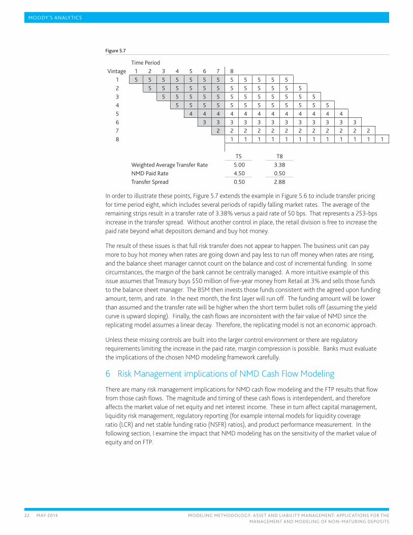
Figure 5.7

Time PeriodVintage 1 2 3 4 5 6 7 8

1 5 5 5 5 5 5 5 5 5 5 5 52 5 5 5 5 5 5 5 5 5 5 5 53 5 5 5 5 5 5 5 5 5 5 5 54 5 5 5 5 5 5 5 5 5 5 5 55 4 4 4 4 4 4 4 4 4 4 4 46 3 3 3 3 3 3 3 3 3 3 3 37 2 2 2 2 2 2 2 2 2 2 2 28 1 1 1 1 1 1 1 1 1 1 1 1

T5 T8Weighted Average Transfer Rate 5.00 3.38NMD Paid Rate 4.50 0.50Transfer Spread 0.50 2.88

In order to illustrate these points, Figure 5.7 extends the example in Figure 5.6 to include transfer pricing for time period eight, which includes several periods of rapidly falling market rates. The average of the remaining strips result in a transfer rate of 3.38% versus a paid rate of 50 bps. That represents a 253-bps increase in the transfer spread. Without another control in place, the retail division is free to increase the paid rate beyond what depositors demand and buy hot money.

The result of these issues is that full risk transfer does not appear to happen. The business unit can pay more to buy hot money when rates are going down and pay less to run off money when rates are rising, and the balance sheet manager cannot count on the balance and cost of incremental funding. In some circumstances, the margin of the bank cannot be centrally managed. A more intuitive example of this issue assumes that Treasury buys $50 million of five-year money from Retail at 3% and sells those funds to the balance sheet manager. The BSM then invests those funds consistent with the agreed upon funding amount, term, and rate. In the next month, the first layer will run off. The funding amount will be lower than assumed and the transfer rate will be higher when the short term bullet rolls off (assuming the yield curve is upward sloping). Finally, the cash flows are inconsistent with the fair value of NMD since the replicating model assumes a linear decay. Therefore, the replicating model is not an economic approach.

Unless these missing controls are built into the larger control environment or there are regulatory requirements limiting the increase in the paid rate, margin compression is possible. Banks must evaluate the implications of the chosen NMD modeling framework carefully.

6 Risk Management implications of NMD Cash Flow Modeling

There are many risk management implications for NMD cash flow modeling and the FTP results that flow from those cash flows. The magnitude and timing of these cash flows is interdependent, and therefore affects the market value of net equity and net interest income. These in turn affect capital management, liquidity risk management, regulatory reporting (for example internal models for liquidity coverage ratio (LCR) and net stable funding ratio (NSFR) ratios), and product performance measurement. In the following section, I examine the impact that NMD modeling has on the sensitivity of the market value of equity and on FTP.


MOODY’S ANALYTICS

6.1 Impact of NMD on Market Value Sensitivity

The sensitivity of market value of equity is one of the primary ALM risk management tools used to measure the interest rate risk of the balance sheet of a bank (see “An Evaluation of Interest Rate Risk Tools and the Future of Asset Liability Management”; Robert J. Wyle; March 2013). Duration is a common fixed income concept that is used to measure the market value sensitivity of a stream of cash flows. The formula for duration of equity is:

Equation 6.1

Where,

DOE = Duration of equity MVA = Market value of assets MVL = Market value of liabilities DA = Duration of assets DL = Duration of liabilities

Therefore, an increase in the duration of deposits causes a decrease in the duration of equity which means that structural balance sheet interest rate risk decreases. Similarly, a decrease in market value of deposits causes an increase in the market value of equity and reduces duration of equity. Therefore, changes in the market value or duration of deposits can have a profound impact on the risk profile of a bank given the importance of NMD as a funding source.

In order to understand the dynamics of the market value sensitivity for NMD, we must revisit the cash flow inputs discussed in section 4. NMD accounts that exhibit low correlation with movements in short rates exhibit higher duration for a given retention as the offered rate responds slowly to movements in market rates (behaves more like a fixed rate instrument). Retention measures how long money remains in an account. For a given correlation to market rates, high retention results in higher duration.

Figure 6.1

Low Retention High Retention

Low Correlation to Market Rates Medium Duration High Duration

High Correlation to Market Rates Low Duration Medium Duration

Figure 6.1 illustrates the impact of the determinants of NMD cash flow on duration. That is, the higher the retention, the higher the duration and the higher the correlation to market rates, the higher the duration.

Figure 6.2: NMD Duration Matrix

Rate Coefficient

Retention 50.00% 40.00% 30.00% 20.00% 10.00%

100.0% 3.94 4.61 5.75 6.94 8.20

90.0% 2.52 2.89 3.51 4.15 4.80

80.0% 1.76 2.00 2.36 2.78 3.17

70.0% 1.31 1.47 1.73 2.00 2.26

60.0% 1.02 1.13 1.32 1.51 1.70

50.0% 0.81 0.90 1.04 1.18 1.32


MOODY’S ANALYTICS

Figure 6.2 illustrates the concepts first explored in Figure 6.1 with a numerical example. The relationship between the rate coefficient and retention on duration are consistent with Figure 6.1.

Now that the link between deposit cash flows and duration has been established, we quantify the impact of changes in deposit duration on net interest income.

Figure 6.3: NMD - Hedge Savings

Rate Coefficient

Retention 50.00% 40.00% 30.00% 20.00% 10.00%

100.0% 26,374 37,586 56,480 76,377 97,360

90.0% 2,635 8,880 19,217 29,823 40,709

80.0% (9,995) (6,033) - 6,953 13,585

70.0% (17,528) (14,805) (10,437) (6,033) (1,593)

60.0% (22,406) (20,435) (17,307) (14,164) (11,004)

50.0% (25,786) (24,313) (21,993) (19,666) (17,330)1 Hedge savings assumes $1.35 million of 10 year equivalence per $10 million of market value change to +200 bps.

Figure 6.3 illustrates how changes in deposit duration can impact net interest income. The hedge savings and added hedge expense required to maintain the same balance sheet duration of equity given the change in deposit duration was plotted in Figure 6.3. Therefore, the ability to measure NMD cash flows can be a significant source of revenue enhancement.

6.2 Impact of NMD on FTP

The strip funding method is an application of valuation in the sense that this method equates the market value of the instrument being transfer-priced with the present value of the cash flows discounted to the funding curve. Therefore, the transfer price represents the economic spread that is accretive to shareholder value. NMD cash flow modeling has a direct impact on FTP because it effects the magnitude and the timing of cash flows which is a major determinant of fair value.

7 Conclusion

There are linkages between the framework for the valuation, interest rate risk quantification, and performance measurement for NMD. The market value falls from the cash flows which, in turn, determine the FTP results. Finally, FTP results derived from both the cash flows and the market values provide incentives to the business lines that determine product management decisions and influence the income statement.

There is a wide range of practice and sophistication across the globe. However, there are advantages to making the underlying deposit modeling assumptions for net interest income (NII) simulation, valuation, and performance management consistent. If they are not consistent, then there could be multiple views of a bank’s risk profile and sub-optimal decision making may result. In addition, bottom-up analysis of the data must be performed to understand the various behavior factors that drive cash flows under various interest rate and economic scenarios.

Both empirical and theoretical NMD behavior models can more accurately quantify the various risk drivers that drive cash flows and better represent the risk profile for the balance sheet of a bank. In addition, the impact of macro-economic factors on deposit retention and decay may be analyzed and modeled independently. The prudent selection and use of advanced NMD modeling techniques can be a source of value creation and return enhancement for a financial institution. Therefore, banks must understand the implications of their modeling approaches and make choices that are consistent with available resources, institution-specific goals, and other constraints.

Further Reading » “An Evaluation of Interest Rate Risk Tools and the Future of Asset Liability Management”; Robert J. Wyle; March 2013

» “Implementing High Value Funds Transfer Pricing Systems”; Wyle and Tsaig; September 2011

MOODY’S ANALYTICS

25 MAY 2014 SP28528/101215/IND-104

© 2014 Moody’s Analytics, Inc. and/or its licensors and affiliates (collectively, ‘MOODY’S’). All rights reserved.

ALL INFORMATION CONTAINED HEREIN IS PROTECTED BY LAW, INCLUDING BUT NOT LIMITED TO, COPYRIGHT LAW, AND NONE OF SUCH INFORMATION MAY BE COPIED OR OTHERWISE REPRODUCED, REPACKAGED, FURTHER TRANSMITTED, TRANSFERRED, DISSEMINATED, REDISTRIBUTED OR RESOLD, OR STORED FOR SUBSEQUENT USE FOR ANY SUCH PURPOSE, IN WHOLE OR IN PART, IN ANY FORM OR MANNER OR BY ANY MEANS WHATSOEVER, BY ANY PERSON WITHOUT MOODY’S PRIOR WRITTEN CONSENT.

All information contained herein is obtained by MOODY’S from sources believed by it to be accurate and reliable. Because of the possibility of human or mechanical error as well as other factors, however, all information contained herein is provided ‘AS IS’ without warranty of any kind. Under no circumstances shall MOODY’S have any liability to any person or entity for (a) any loss or damage in whole or in part caused by, resulting from, or relating to, any error (negligent or otherwise) or other circumstance or contingency within or outside the control of MOODY’S or any of its directors, officers, employees, or agents in connection with the procurement, collection, compilation, analysis, interpretation, communication, publication, or delivery of any such information, or (b) any direct, indirect, special, consequential, compensatory, or incidental damages whatsoever (including without limitation, lost profits), even if MOODY’S is advised in advance of the possibility of such damages, resulting from the use of or inability to use, any such information. The ratings, financial reporting analysis, projections, and other observations, if any, constituting part of the information contained herein are, and must be construed solely as, statements of opinion and, not statements of fact or recommendations to purchase, sell, or hold any securities.

NO WARRANTY, EXPRESS OR IMPLIED, AS TO THE ACCURACY, TIMELINESS, COMPLETENESS, MERCHANTABILITY OR FITNESS FOR ANY PARTICULAR PURPOSE OF ANY SUCH RATING OR OTHER OPINION OR INFORMATION IS GIVEN OR MADE BY MOODY’S IN ANY FORM OR MANNER WHATSOEVER.

Each rating or other opinion must be weighed solely as one factor in any investment decision made by or on behalf of any user of the information contained herein, and each such user must accordingly make its own study and evaluation of each security and of each issuer and guarantor of, and each provider of credit support for, each security that it may consider purchasing, holding, or selling.

Any publication into Australia of this document is pursuant to the Australian Financial Services License of Moody’s Analytics Australia Pty Ltd ABN 94 105 136 972 AFSL 383569. This document is intended to be provided only to ‘wholesale clients’ within the meaning of section 761G of the Corporations Act 2001. By continuing to access this document from within Australia, you represent to MOODY’S that you are, or are accessing the document as a representative of, a ‘wholesale client’ and that neither you nor the entity you represent will directly or indirectly disseminate this document or its contents to retail clients within the meaning of section 761G of the Corporations Act 2001.

asset and liability management: applications for the … · asset and liability management:...

Documents