assessment using the weibull-markov...
TRANSCRIPT

P r 0 1
P r 1 0
P r 1 2P r 2 1
P r 2 0
P r 0 2
h o , b 0
h 1 , b 1
h 2 , b 2
S t a t e 0S t a t e 1
S t a t e 2
Power System ReliabilityAssessment using theWeibull-Markov Model
JASPER VAN CASTEREN
Department of Electric Power EngineeringCHALMERS UNIVERSITY OF TECHNOLOGY
Göteborg, Sweden, 2001

Thesis for the degree of Licentiate of Engineering
Technical Report No. 381L
Power system reliability assessment using theWeibull-Markov model
by
Jasper van Casteren
Department of Electric Power EngineeringChalmers University of Technology
S-412 96 Göteborg, Sweden
Göteborg 2001

Power system reliability assessment using the Weibull-Markov model
This thesis has been prepared using LATEX.
Copyright ©2001, Jasper van Casteren.All rights reserved.
Jasper van CasterenPower system reliability assessment using theWeibull-Markov model.Technical Report No. 381L.Licenciate Thesis.
Printed in Sweden.
Chalmers ReproserviceGöteborg 2001

Dedicated to Wille


Preface
This thesis introduces the Weibull-Markov model as an alternative to thewidely used homogenous Markov model. Such alternatives are likely tomeet a lot of scepticism. This is understandable, because the homogenousMarkov models are rooted in complex stochastic theory and have been usedto great success in all areas of reliability calculations for a long time. To eventhink of developing a serious alternative in the course of a PhD project, andthen even to do this as an electrical engineer, must seem to be at least naive.
Yet, the work presented here is not believed to be in vain. Although it tooksome time to get the mathematical equations in a form that seems to bebearable for real mathematicians, the principle idea behind them survivedthrough the process of testing, checking and implementation. This givesgood hope for the future of the Weibull-Markov model.
This Licenciate Thesis would not have been made possible without the con-structive cooperation between the Chalmers University in Sweden and theDIgSILENT company in Germany.
Göteborg, Sweden, 27.02.2001,Jasper van Casteren

Abstract
This Licenciate Thesis introduces an alternative stochastic model for per-forming reliability assessment calculations in electric power systems. Thisnew model has been developed because the commonly used “homogenousMarkov” model cannot be used to calculate cost parameters accurately. Yet,the current market developments lead to an increasing demand for cost-oriented reliability assessment.
The proposed alternative model, which was given the name “Weibull-MarkovModel”, has been implemented and used in a commercial reliability assess-ment program with success. The use of the new model has proven not tocause any relevant slowing down of the calculation process, and yet to de-liver reliability cost indices at the same time. Additional reliability calculationsfor cost calculations therefore are felt not to be required anymore.
A very important quality of the Weibull-Markov model is that it is 100% back-wards compatible with the homogenous Markov model. This means that thereliability data that has been gathered to great costs and effort in the past,can still be used in the new calculations. The Weibull-Markov model pro-vides for a so-called shape parameter with wich an existing homogenousMarkov model can be adjusted to bring it closer to the measured data with-out actually changing the original data.
More research however will be needed to test the Weibull-Markov modelfurther for its merits and limits.


Contents
1 Power System Reliability Assessment 1
2 Stochastic models 42.1 Stochastic Models . . . . . . . . . . . . . . . . . . . . . . . . 6
2.1.1 The Exponential Distribution . . . . . . . . . . . . . . 92.1.2 The Weibull distribution . . . . . . . . . . . . . . . . . 102.1.3 Weibull Probability Charts . . . . . . . . . . . . . . . . 112.1.4 Lifetime, Repair and Failure Density . . . . . . . . . . 12
2.2 Homogenous Markov Models . . . . . . . . . . . . . . . . . . 142.2.1 The Homogenous Markov Component . . . . . . . . . 152.2.2 The Homogenous Markov System . . . . . . . . . . . 192.2.3 Interruption Costs Calculations . . . . . . . . . . . . . 232.2.4 Device of Stages . . . . . . . . . . . . . . . . . . . . . 26
2.3 Weibull-Markov Models . . . . . . . . . . . . . . . . . . . . . 282.3.1 Component State Probability and Frequency . . . . . 32
2.4 The Weibull-Markov System . . . . . . . . . . . . . . . . . . . 342.4.1 Weibull-Markov System State Probability and Frequency 352.4.2 Weibull-Markov System State Duration Distribution . . 37
2.5 Basic Power System Components . . . . . . . . . . . . . . . 422.5.1 Defining a Weibull-Markov Model . . . . . . . . . . . . 422.5.2 A Generator Model . . . . . . . . . . . . . . . . . . . . 44
3 Applications / Examples 483.1 Comparison with Monte Carlo Simulation . . . . . . . . . . . 483.2 Small System Example . . . . . . . . . . . . . . . . . . . . . 493.3 Larger System Example . . . . . . . . . . . . . . . . . . . . . 52
i
4 Conclusions 58
A Glossary of Terms 59

Terms and Abbreviations
Terms
���� ����� central moment of D � variance of D � standard variance of D� � ��������� remainder CDF for ��� ����Stochastic component ������ �! "#�
’th successive state of�$�
% ��� �! "#�’th successive epoch at which
�$�changes
� ��� & duration of���('*)
+ ��� &-,homogenous transition rate for
�$�.'*)to���.'0/
+ ��� &homogenous state transition rate for
�1�.'*)2
Stochastic system2 �43 "#5’th successive state of
2%6�43 " 5
’th successive epoch at which2
changes����� �43 ���according to
2 �43����� 5 ���
according to2 '87
� � � "#5 � Remaining duration of�$��� �43
at% �43
9 � � "#5 � Passed duration of�$��� �43
at% �43
: ��� & Weibull form factor for�$�.'*)
; ��� &Weibull shape factor for
�$�.'*)�<��� &
Mean duration of�$�.'*)
=��� &Variance of the duration of
�$�.'*)> ��� �43
=> ��� &
for����� �43('*)
, i.e. : ��� �43 , ; ��� �43 , etc.> ��� 5=> ��� &
for����� 5?'*)
, i.e. : ��� 5 , ; ��� 5 , etc.@BAC��� &Frequency of occurrence of
�$�.'*)DEAF��� &
Probability of occurrence of�$�.'*)
@BAC5Frequency of occurrence of S=sDEAF5Probability of S=s

Abbreviations
TTF Time To FailureTTR Time To RepairMTBF Mean Time Between FailuresTBM Time Between MaintenanceCDF Cumulative Density FunctionPDF Probability Density FunctionSF Survival Function

Chapter 1
Power System ReliabilityAssessment
The assessment of the reliability of a power system means the calculation ofa set of performance indicators. An example of such an indicator is the av-erage number of times per year that a certain load point cannot be suppliedwith electrical energy. Basically, there are two distinct sets of indicators: lo-cal indicators and system indicators. Local indicators are calculated for aspecific point in the system. Examples are
• The average time per year during which a generator is not able to feedinto the network
• The average duration of the interruptions at a busbar.
• The average interruption costs per year for a specific load.
System indicators express the overall system performance. Examples are
• The average amount of energy per year that cannot be delivered to theloads.
• the average number of interruptions per year, per customer.
• The average yearly interruption costs.
Power system reliability analysis is principally the analysis of a large set ofunwanted system states which may occur in the future. The results of all
1

Power System Reliability Assessment
these system state analyses is then used to calculate the various perfor-mance indicators. The basic diagram of the calculation procedure is de-picted in Fig. 1.1. This diagram shows the healthy operational state of thesystem, in which all components behave properly. The reliability assess-ment creates events that will bring the system in an unhealthy state, whichis then analyzed. When this analysis shows that the system is not longerable to meet all its demands, a set of intermediate results is send to a resultanalyzer. This is repeated for all relevant unhealthy system states. Finally,the result analyzer will post-process the gathered results in order to calcu-late the various performance indicators.
healthy operational state
events
Failure Effect Analysis
result analyser
results
Figure 1.1: Basic reliability assessment scheme
The reliability assessment process thus starts with the creation of relevantsystem events. This must be done in such a way as to make it possible toweight the results of the failure effect analysis. Not every event is equallylikely to happen, and the more likely events will have a greater impact on theperformance indices than the less likely ones. Creating weighted events ismade possible by the use of stochastic component models. These modelsare combined in system models and are used to create system states in spe-cific orders and to calculate the frequency and probability of the occurrenceof these system states.
This licenciate thesis introduces the basic methodologies for creating andusing stochastic models, and will introduce the wide-spread and commonly
2

Power System Reliability Assessment
used homogenous Markov model and the alternative Weibull-Markov model.
3

Chapter 2
Stochastic models
In order to calculate reliability performance indicators, the analyzed powersystem has to be represented by stochastic models first. An electrical powersystem is regarded as a collection of components. Each component is a typ-ical part of the electric power system which is treated as one single object inthe reliability analysis. Examples are a specific load, a line, a generator, etc.,but also a complete transformer bay with differential protection, breakers,separators and grounding switches may be treated as a single componentin a reliability assessment.
A component may exhibit different ’component states’, such as ’being avail-able’, ’being repaired’, etc. In the example of a transformer, the followingstates could be distinguished:
1. the transformer performs to its requirements
2. the transformer does not meet all its requirements
3. the transformer is available, but not used
4. the transformer is in maintenance
5. the transformer is in repair
6. the transformer is being replaced by another transformer
7. the transformer behaves in such a way as to trigger its differential relay
4
Stochastic models
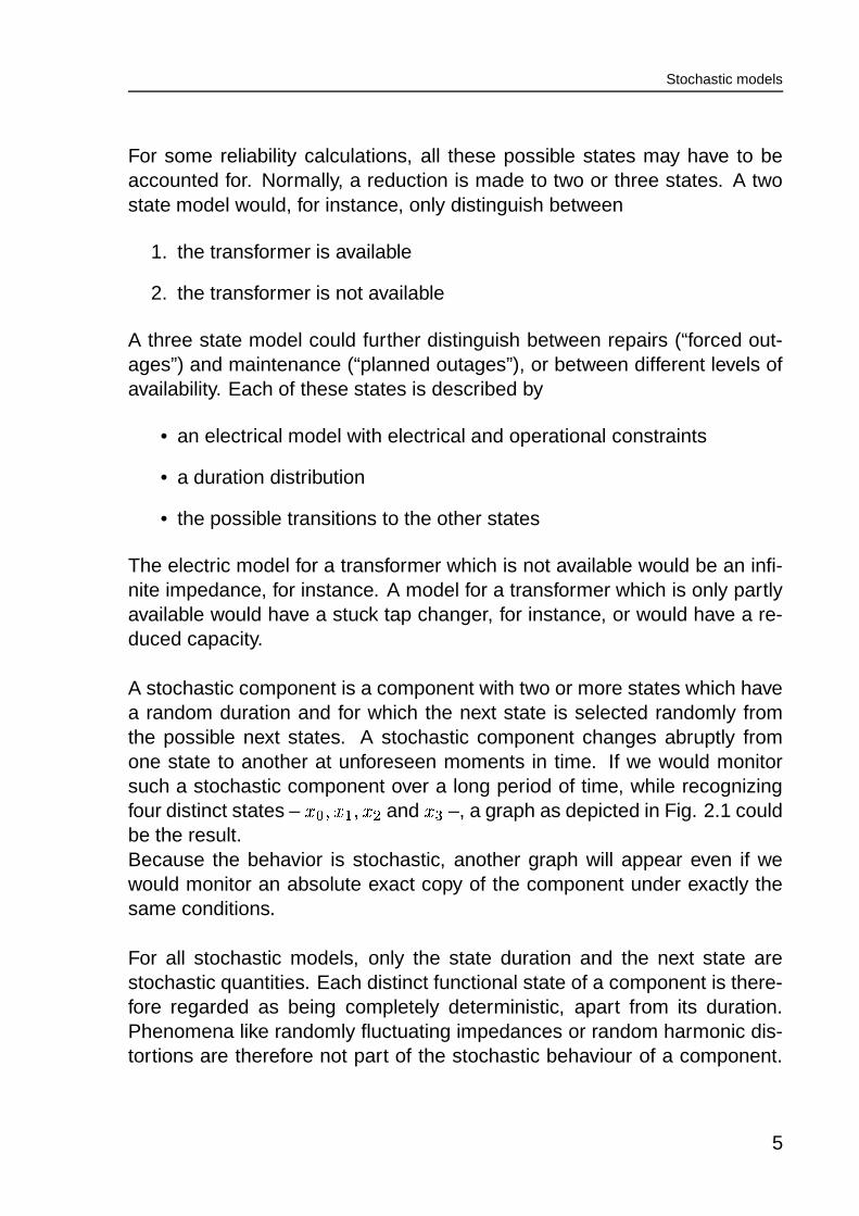
For some reliability calculations, all these possible states may have to beaccounted for. Normally, a reduction is made to two or three states. A twostate model would, for instance, only distinguish between
1. the transformer is available
2. the transformer is not available
A three state model could further distinguish between repairs (“forced out-ages”) and maintenance (“planned outages”), or between different levels ofavailability. Each of these states is described by
• an electrical model with electrical and operational constraints
• a duration distribution
• the possible transitions to the other states
The electric model for a transformer which is not available would be an infi-nite impedance, for instance. A model for a transformer which is only partlyavailable would have a stuck tap changer, for instance, or would have a re-duced capacity.
A stochastic component is a component with two or more states which havea random duration and for which the next state is selected randomly fromthe possible next states. A stochastic component changes abruptly fromone state to another at unforeseen moments in time. If we would monitorsuch a stochastic component over a long period of time, while recognizingfour distinct states – ��� � ��� � ��� and ��� –, a graph as depicted in Fig. 2.1 couldbe the result.Because the behavior is stochastic, another graph will appear even if wewould monitor an absolute exact copy of the component under exactly thesame conditions.
For all stochastic models, only the state duration and the next state arestochastic quantities. Each distinct functional state of a component is there-fore regarded as being completely deterministic, apart from its duration.Phenomena like randomly fluctuating impedances or random harmonic dis-tortions are therefore not part of the stochastic behaviour of a component.
5

Stochastic models
T n
X n
x 0
x 1
x 2
x 3
t 0 t 1 t 2 t 3 t 4 t 5
Figure 2.1: Example of monitored states of a component
If such phenomena are to be included in a reliability assessment, to assessthe number of interruptions due to excessive harmonic distortion for exam-ple, the stochastic model must be extended by a number of states for whichthe fluctuating random quantity is considered constant.
This chapter introduces the stochastic models for electrical power systemcomponents. From these stochastic models, the model for a stochasticpower system are then developed.
2.1 Stochastic Models
The basic quantity in reliability engineering is the duration � for which acomponent stays in the same state. This duration is a stochastic quantity,as its precise value is unknown. The word “precise” is emphasized here, as,although we don’t know the value of a stochastic quantity, we almost alwaysknow something about the possible values it could have. The time until thenext unplanned trip of a generator, for example, is unknown, but nobodywould expect a good generator to trip every day, as well as nobody wouldexpect it to operate for 10 years continuously without tripping even once.This example range from 1 day to 10 years is too wide to be of practicaluse in a reliability assessment. However, for actual generators, a muchsmaller range of expected values can be justified by using measured data.The basic question about a stochastic quantity is thus about the range of itsexpected values, or ‘outcomes’: which outcomes can be expected and withwhat probability?
6
Stochastic models
Both the outcome range and the outcome probabilities can be described bya single function; the “Cumulative Density Function” or CDF. This functionis written as
� � ����� and defines the probability of � being smaller than � ,which is written as:
� � ����� ' DEA � ��� ��� (2.1)
for reliability purposes, the probability for a negative duration is zero and theprobability that the duration will be smaller than infinity is one:
� � ��� � ' � (2.2)� � ��� � ' �(2.3)
The “Probability Density Function”, or PDF, for � , � � ����� , is the derivativeof the cumulative density function. The PDF gives a first insight into thepossible values for � , and the likelihood of it taking a value in a certainrange.
� � ����� ' � � � ����� (2.4)
� � ����� ' ��� ����� �DEA ��� � ��� ����� ���� � (2.5)���
�� � ����� � ' ��� � (2.6)
The survival function (SF), � � ����� , is defined as the probability that the du-ration � will be longer than � .
� � ����� ' DEA � ��� ��� '��! "� � ����� (2.7)
For a specific component, i.e. a transformer, where � is the life time, whichis also known as the time to failure (TTF), the survival function gives theprobability for the component functioning for at least a certain amount oftime without failures. For a large group of similar components, the SF isthe expected fraction of components that will ‘survive’ up to a certain timewithout failures.
7
Stochastic models
The hazard rate function (HRF),� � ����� , is defined as the probability density
for a component to fail, for a certain time � , given the fact that the componentis still functioning at � ,
� � ����� ' ��� ����� �DEA ��� � ��� � ��� ��� � � ���� � ' � � ������ � ����� (2.8)
The HRF is an estimate of the unreliability of the components that are stillfunctioning without failures after a certain amount of time. An increasingHRF signals a decreasing reliability. An increasing HRF means that theprobability of failure in the next period of time will increase with age. Adecreasing HRF could, for instance, occur when only the better componentssurvive.
The expected value of a function � of a stochastic quantity � is defined as
� � � � � ��� '����� ����� � � ����� � (2.9)
The expected value of D itself is its mean� � , which is defined as
� � '�� � � � '����
� � � ����� � (2.10)
The k’th central moment,� �� , is defined as� �� '�� ��� � �� � � � � � (2.11)
The variance � is defined as the second central moment � ' � �� '�� ��� � �� � � � � � '�� � � � � � � � � ��� � (2.12)
The standard variance � is defined as the square of the variance � '�� � (2.13)
The remainder CDF is defined as the CDF of the remaining duration after aninspection moment � . Because the total duration � is a stochastic quantity,the remainder � � is also stochastic. The remainder CDF,
� � ���=����� , isdefined as
� � ���=����� ' DEA � ��� � � ��� ��� ' DEA ��� � ��� ���DEA ��� � � �' � � ����� "� � �����
� � ����� (2.14)
8
Stochastic models
2.1.1 The Exponential Distribution
The negative exponential distribution is defined by
� � ����� ' + ����� � (2.15)
which makes that
� � ����� ' �! ����� � (2.16)� � ����� ' +
(2.17)� � ' �
+ (2.18)
� ' �+ � (2.19)
The HRF of the negative exponential distribution,� � ����� , is not dependent of
time which considerably simplifies many reliability calculations.
The remainder CDF,��� ���=����� , for the negative exponential distribution equals
� � ���=����� '��! ������� � � � ' � � ��� ��� (2.20)
The remainder of an exponential distributed duration thus has the same dis-tribution as the total duration. The expected value, variance, etc. for theremainder thus equal those of the total duration, independent of the inspec-tion time. This is a peculiarity unique to the negative exponential distribution.It also shows that the negative exponential distribution is a very abstract dis-tribution. If, for instance, a repair duration would be negative exponentiallydistributed, then the expected time to finish the repair would be independentof the time already spend repairing. Such a type of repair is hard to imagine.An example of a duration that is negative exponentially distributed is the timeit takes to throw 9 sixes with 9 dice, with a throw about every 3 seconds. Inthis way, a throw of 9 sixes will occur about once a year, on average, butthe expected time until the next 9 sixes will always be about 1 year as theprobability of 9 sixes in the next throw is independent of the number of trialsdone so far.
9

Stochastic models
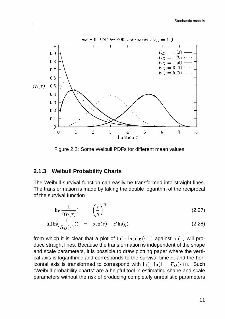
2.1.2 The Weibull distribution
Where the exponential distribution uses only one parameter (+), the Weibull
PDF uses a shape factor;
and a scale factor : . It is defined as
� � ����� ' ;: � � � � ��������� � :�� �� (2.21)
which makes that
� � ����� ' �! ������� � : � �� (2.22)
� � ����� ' ;: � � � � � (2.23)
� � ' :�� � � �; � (2.24)
� ' : ��� � � ���; � �� � � � �; ��� ��� (2.25)
where� � � � ' ����
��� � � ��� � �is the normal gamma function.
The Weibull PDF equals the negative exponential distribution when the shapeparameter
; '���� � . The gamma function which is needed for calculating theexpected value and variance can be evaluated without much computationaleffort by standard numerical methods. Some examples of the Weibull PDF,for different means and variance are displayed in in Fig. 2.2 and Fig. 2.3.The conditional CDF,
� � ���=����� , for the Weibull distribution equals
� � ���=����� ' ����� � �: � � � : � � (2.26)
which is dependent on the inspection time � .
10
Stochastic models
�
�����
�����
�����
���
����
�����
��� �
�����
�����
�
� � � � � � �
� � �����
��������������� �
� � ��!���"�"$#&%('*)+�,�-�.�0/ � � � ���21 � �,��354 � '���� �� � '���� ���� � '���� � 6� � '���� 6 �� � '87 � ���� � ' 6 � ���
Figure 2.2: Some Weibull PDFs for different mean values
2.1.3 Weibull Probability Charts
The Weibull survival function can easily be transformed into straight lines.The transformation is made by taking the double logarithm of the reciprocalof the survival function
:9 � �� � ����� � ' � :�� � (2.27)
:9 � :9 � �� � ����� ��� ' ; :9 ����� ; :9 � : � (2.28)
from which it is clear that a plot of:9 � :9 � � � ��������� against
:9 ����� will pro-duce straight lines. Because the transformation is independent of the shapeand scale parameters, it is possible to draw plotting paper where the verti-cal axis is logarithmic and corresponds to the survival time � , and the hor-izontal axis is transformed to correspond with
:9 � :9 � � � � ��������� . Such“Weibull-probability charts” are a helpful tool in estimating shape and scaleparameters without the risk of producing completely unrealistic parameters
11
Stochastic models
�
������
�����
�����
�����
�����,
�����
������
���
���
� � � � � �
� � �����
��������������� �
� � ��!���"�"$#&%('*)+�,�-�.�0/ � � � ��� � � �����,��� � 3 4 � � '�� � � � � '���� � � ' � � � � '87 � � � ' 6 � �
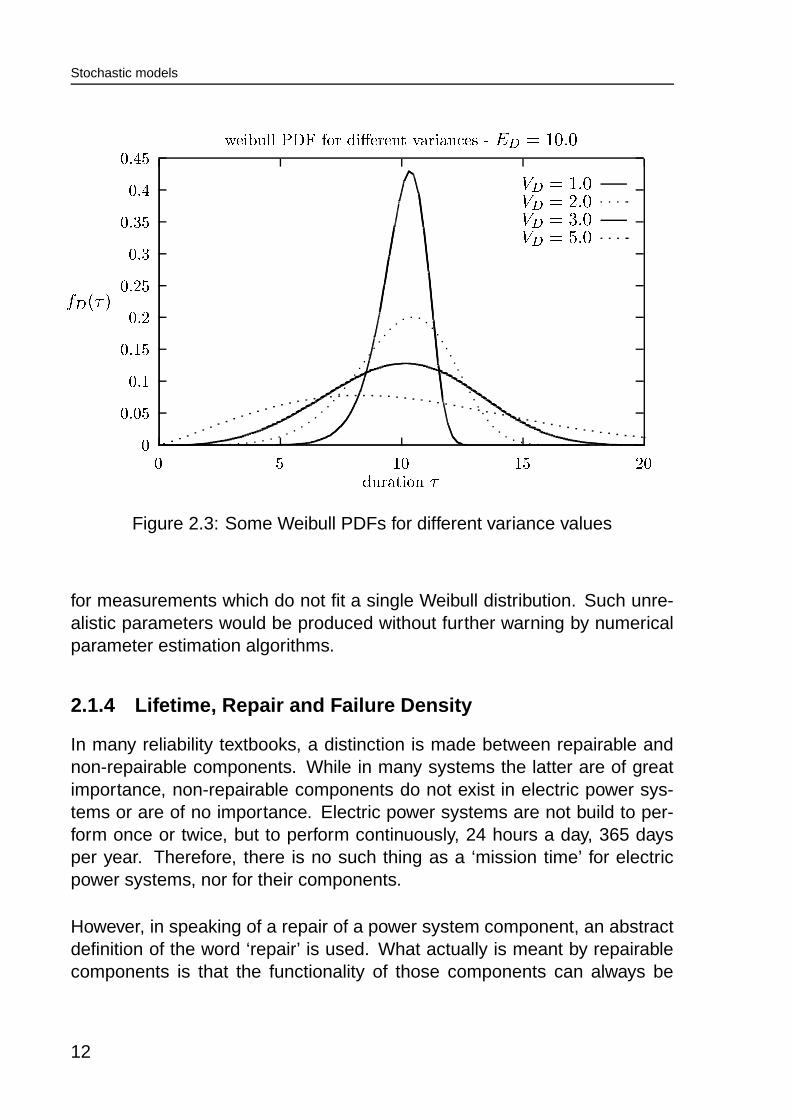
Figure 2.3: Some Weibull PDFs for different variance values
for measurements which do not fit a single Weibull distribution. Such unre-alistic parameters would be produced without further warning by numericalparameter estimation algorithms.
2.1.4 Lifetime, Repair and Failure Density
In many reliability textbooks, a distinction is made between repairable andnon-repairable components. While in many systems the latter are of greatimportance, non-repairable components do not exist in electric power sys-tems or are of no importance. Electric power systems are not build to per-form once or twice, but to perform continuously, 24 hours a day, 365 daysper year. Therefore, there is no such thing as a ‘mission time’ for electricpower systems, nor for their components.
However, in speaking of a repair of a power system component, an abstractdefinition of the word ‘repair’ is used. What actually is meant by repairablecomponents is that the functionality of those components can always be
12
Stochastic models
restored, even when this means that the physical hardware (the appliance)is completely replaced.
A repair can restore the component to a condition as if it was brand newagain. Repair by replacement is the trivial example. Such a perfect repairis called a repair-as-good-as-new. If the repair restores the component toabout the same condition in which it was directly before the failure, it is calleda repair-as-bad-as-old. Normally, repairs in between maintenance, whichare often performed under great time pressure, are repairs-as-bad-as-old.Maintenance is normally considered to be a repair-as-good-as-new.
Components will normally start their life ready for use, i.e. with availablefunctionality, and as-good-as-new. This is called their ‘NEW’ state. As soonas they are taken into service they will age and they will no longer be in their‘NEW’ state. However, as long as they perform to expectation they are saidto be in their ‘UP’ state. A component may fail at some time after it has beentaken into service. This time is called the Time To Failure or TTF.
Ideal Maintenance
Non-repairable components will function until they fail. After that, their life isover. Although an electrical power system will never exhibit non-repairablecomponents, their behaviour is of theoretical interest.
The life-time of non-repairable components may be prolonged by preven-tive maintenance. A preventive maintenance restores the component to thestate ‘as good as new’, if it was still functioning. If we schedule maintenanceat fixed intervals
% � , we can calculate the new PDF for the time to failure forthe maintained component.
The probability density for the period until the first maintenance, � � ����� , hasthe same shape as the original PDF because maintenance has not changedanything yet:
� � ����� '� � � ����� if � � � � % �� � � � ����� )�7 � (2.29)
Note the fact that � � ����� is strictly speaking not a PDF, because it only de-scribes the distribution in the first period and � �� � � ����� � will therefore be
13

Stochastic models
smaller than one.
The probability of surviving until � ' % � is � � � % � � . This is also the probabil-ity of the component to fail at � � % � if the maintenance would not have beenperformed. When the duration of the maintenance is neglected here, whichis acceptable because it will normally be much smaller than
% � , then thisremaining probability is distributed over all moments � � % � . The shape ofthe distribution is again the same as the original because the maintenance isa repair-as-good-as-new. The probability distribution for the second periodwill therefore be
� � ����� '� � � � % � � � � ��� % � � if
% � � � � � % �� � � � ����� )�7 � (2.30)
The general solution is achieved by repeating this for � ' � % � with � �����(see [36, p.14])
���� ����� '���� � �
�� � % � � � � ��� � % � � (2.31)
This is an important result, because the geometric expression � �� � % � � forcesthe PDF to fluctuate between two negative exponential curves. Therefore,we would expect the failure rate to become more or less constant for higher� , regardless of the original shape of the PDF. This is an important result,because it shows that measurements of the time to failure should measurethe time from the end of the last maintenance to the moment of failure, andnot as the time between failures. Interpreting time between failures as a TTFwill lead to a stochastic model with negative exponentially distributed dura-tions, which would not represent the component itself, but the combinationof the component and the planned maintenance. Such models can not beused for determining the effects of changed maintenance planning.
2.2 Homogenous Markov Models
One of the important qualities of the homogenous Markov model is that itcauses each stochastic system build from homogenous Markov models tobe a homogenous Markov model again, only much larger. This enables the
14
Stochastic models
calculation of state probability, frequency and duration by analytic matrix op-erations. Although this seems to be a great advantage, this is only partlyso, because the calculation of system state indices is often much easier byadding the contributions of the system components. The one exception isthe calculation of system state duration distributions, but these distributions,although easily obtained for a homogenous Markov system model, will beunrealistic in such a model. This is so because the one important disadvan-tage of the homogenous Markov model is the exclusive use of the negativeexponential distribution for all stochastic durations in the system. In the caseof repair of maintenance durations, these distributions are already highly un-likely, but in the case of life time, they cannot be other than incorrect. Usinga negative exponentially distributed lifetime will always cause the model toreact to preventive maintenance by a lowered overall availability, which issurely not the case for normal power system equipment.
Nevertheless, the homogenous Markov model is very important due to itscomputational elegance. A good understanding of the basic properties ofthe homogenous Markov model is required for understanding other modelsand methods used in power system reliability assessment.
2.2.1 The Homogenous Markov Component
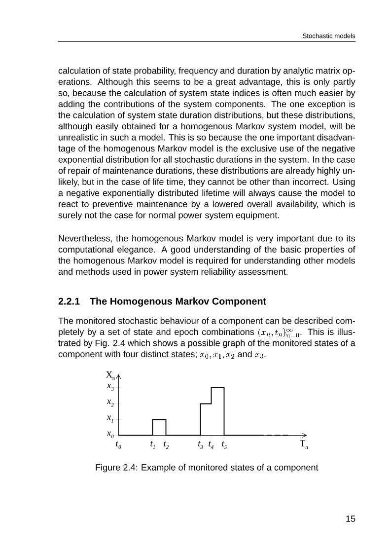
The monitored stochastic behaviour of a component can be described com-pletely by a set of state and epoch combinations � � � ��� � � �� � � . This is illus-trated by Fig. 2.4 which shows a possible graph of the monitored states of acomponent with four distinct states; � � � ��� � ��� and ��� .
T n
X n
x 0
x 1
x 2
x 3
t 0 t 1 t 2 t 3 t 4 t 5
Figure 2.4: Example of monitored states of a component
15

Stochastic models
If we would monitor the exact same component under exact the same condi-tions, another set � � � ��� � � �� � � will be the result, as each next state and eachstate duration ��� � � � � � � are stochastic quantities. Each set � � � ��� � � �� � � is anoutcome from a infinite number of possible outcomes, and is called a “com-ponent history”. The stochastic history for the component with index “c”, iswritten as “ � �$��� �! � % ��� �! � ��! � � ”. Both
����� �! and
% ��� �! are stochastic quantities
and we may talk, for example, about “the probability of�1��� � � ' ��� ” or “the
probability density function of � % ��� ��� % ��� ��� � ”.The homogenous Markov model is now defined by:
• the set of possible states � � '�� � � � �������6�� �� where � � is the numberof possible states
• the stochastic history � �$��� �! � % ��� �! � ��! � � , where
– � �! � ����� �! � � � � ����� �! � '*����� �! � � �–% ��� � ' � and � �! � % ��� �! � � � % ��� �! �
• the set of continuous probability distribution functions� ��� &-, ����� for the
conditional state durations � ��� &-,� ��� &-, ����� ' DEA � � ��� &-, � ���
' DEA � ����� �! .'*) � � % ��� �! � � % ��� �! � � � � ����� �! � � '0/ �' �! ����� �+ ��� &-, �
From the homogenous Markov model, the stochastic process� � ����� can be
defined as
% ��� �! � � � % ��� �! � ��� ��� ����� '*����� �! (2.32)
The conditional state durations � ��� &-, are the stochastic durations for state), given the fact that the next state will be
/. An outcome of a history is
obtained by drawing outcomes ��� & � for all conditional state durations � ��� & � ineach state, and selecting the smallest value. Then, with
/such that ��� &-, ' �:9 � ��� & � � , ����� �! � � '0/
and% ��� �! � � ' % ��� �! � ��� &-, .
16

Stochastic models
The probability distribution for the duration � ��� & of state � ��� & is thus the distri-bution of the minimum of the conditional durations:
� ��� & ����� ' DEA � � ��� & � ��� ' DEA � � �:9, � � � � ��� &-, � � ���
' �! � �, � �
DEA � � ��� &-, � ��� '��! � �, � �
����� �+ ��� &-, �' �! ����� �+ ��� & � (2.33)
�+ ��� & ' �
�, � �
�+ ��� &-, (2.34)
The state duration is thus again exponentially distributed and is character-ized by the single ‘state transition rate’
+ ��� &. The state transition rate is ex-
pressed in ‘per time’ units, and may thus be interpreted as a frequency. Thisfrequency, however, expresses the number of transitions out of the state pertime spend in the state, and not per total time. The state transition rate thusonly equals the state frequency for a component with just one state. Fora component with two identical states, the state frequency will be half thestate transition rate. The expected state duration can be directly calculatedfrom the state transition rate as
� � � ��� & � '�+ ��� & (2.35)
For the transition probability � � � ) � / � ' DEA � ����� �! � � ' / � ����� �! ' ) � it followsthat
� � � ) � / � ' DEA � � ��� &-, '� �:9�� � � � ��� & � ���
' ����
DEA � �:9���� , � � ��� & � ����� � �+ ��� &-, ����� � � ��� �
' � ��
�+ ��� &-, ����� � � � �
' + ��� &+ ��� &-, (2.36)
Both the state duration distribution and the transition probabilities are thusindependent of time and independent of the history of the system. By
17
Stochastic models
(2.36), a constant transition probability matrix � � ' � � � � ) � / � is defined forthe Markov model. The fact that the transition probabilities are constantmeans that the sequence of states in a history of the component is indepen-dent of the time spend in those states. This sequence of states, � � ��� �! � ��! � � ,is called the “embedded Markov chain”. For Markov chains with stationarytransition probabilities the so-called Markov-property holds, which can bewritten as
DEA � ����� �! � � '0/ � ����� � ' � � ����� � '�� ������� � ����� �! '*) � (2.37)' DEA � ����� �! � � '0/ � ����� �! .'*) � ' � � � � � ) � / �
where � � � � � ) � / � is the value on the) � / position in the � ��� power of � � . For
all � � � �, � &�� � , � � � � � � ) � / � '���� � .
The Markov property tells us that the probability to find the component ina certain state after a certain number of transitions only depends on thenumber of transitions and on the starting state.
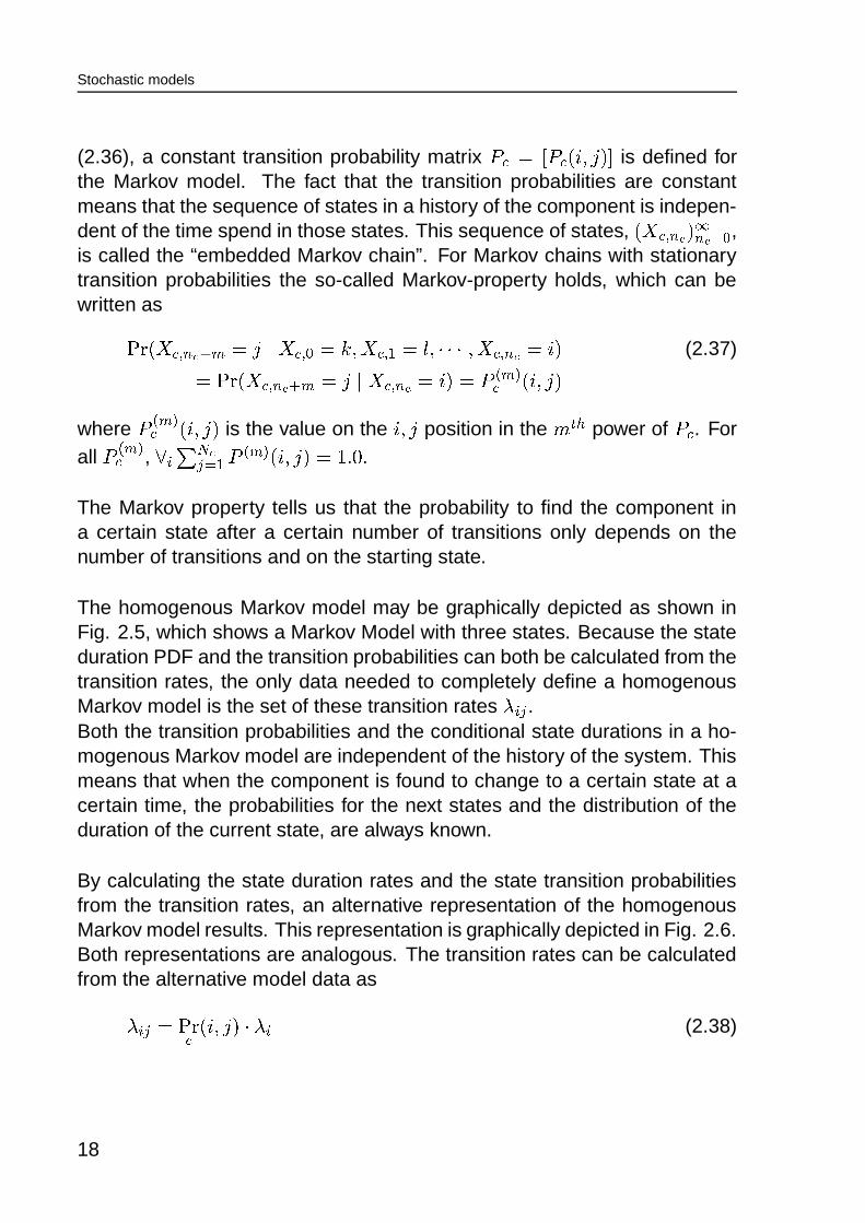
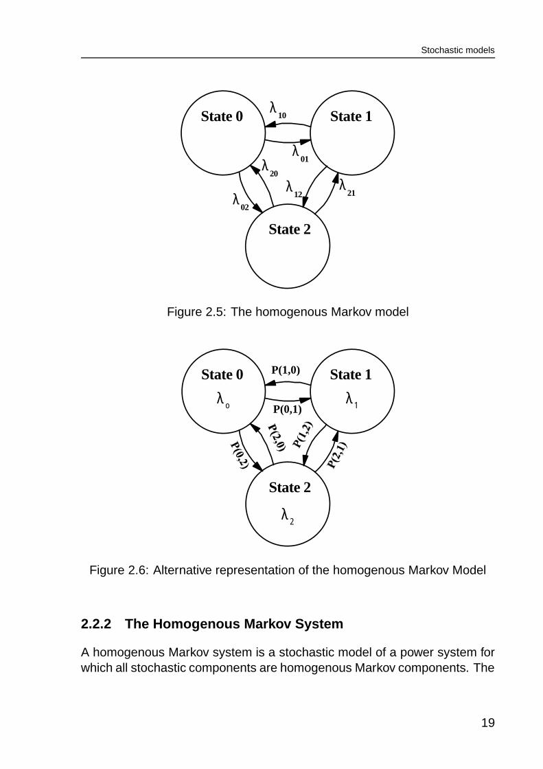
The homogenous Markov model may be graphically depicted as shown inFig. 2.5, which shows a Markov Model with three states. Because the stateduration PDF and the transition probabilities can both be calculated from thetransition rates, the only data needed to completely define a homogenousMarkov model is the set of these transition rates
+ &-,.
Both the transition probabilities and the conditional state durations in a ho-mogenous Markov model are independent of the history of the system. Thismeans that when the component is found to change to a certain state at acertain time, the probabilities for the next states and the distribution of theduration of the current state, are always known.
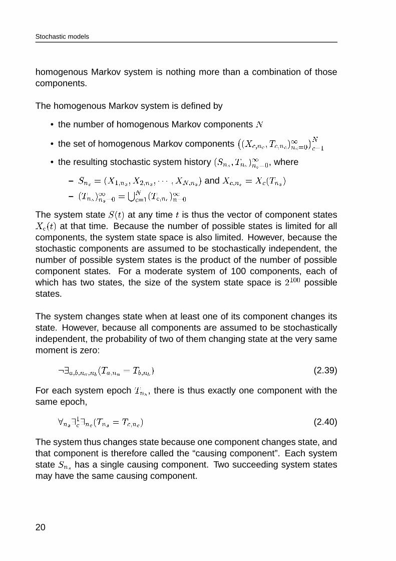
By calculating the state duration rates and the state transition probabilitiesfrom the transition rates, an alternative representation of the homogenousMarkov model results. This representation is graphically depicted in Fig. 2.6.Both representations are analogous. The transition rates can be calculatedfrom the alternative model data as
+ &-, ' DEA� � ) � / � � + & (2.38)
18
Stochastic models
λ 01
λ 10
λ 21 λ
12
λ 20
λ 02
State 0 State 1
State 2
Figure 2.5: The homogenous Markov model
P(0,1)
P(1,0)
λ ο λ 1
λ 2
State 0 State 1
State 2
Figure 2.6: Alternative representation of the homogenous Markov Model
2.2.2 The Homogenous Markov System
A homogenous Markov system is a stochastic model of a power system forwhich all stochastic components are homogenous Markov components. The
19
Stochastic models
homogenous Markov system is nothing more than a combination of thosecomponents.
The homogenous Markov system is defined by
• the number of homogenous Markov components �
• the set of homogenous Markov components� � ����� �! � % ��� �! � ��! � ��� �� � �
• the resulting stochastic system history � 2 �43 � % �43 � ��43 � � , where
–2 �43(' � � � � �43 � � � � �43 ������� � � � � �43 � and
����� �43('*��� � % �43 �– � % �43 � ��43 � � '�� �� � � � % ��� �! � �� � �
The system state2 ����� at any time � is thus the vector of component states��� ����� at that time. Because the number of possible states is limited for all
components, the system state space is also limited. However, because thestochastic components are assumed to be stochastically independent, thenumber of possible system states is the product of the number of possiblecomponent states. For a moderate system of 100 components, each ofwhich has two states, the size of the system state space is � � � � possiblestates.
The system changes state when at least one of its component changes itsstate. However, because all components are assumed to be stochasticallyindependent, the probability of two of them changing state at the very samemoment is zero:
���� � �� ��� � �� � % � � ��� ' % �� �� � (2.39)
For each system epoch% �43
, there is thus exactly one component with thesame epoch,
� �43 � �� � �! � % �43(' % ��� �! � (2.40)
The system thus changes state because one component changes state, andthat component is therefore called the “causing component”. Each systemstate
2 �43has a single causing component. Two succeeding system states
may have the same causing component.
20
Stochastic models
For a system which changes to state2 �43
at time% �43
, the remaining stateduration for component � is defined as
� � � "#5 � ' % ��� �43� � � % �43 (2.41)"#5 � ' ���� � "#� ��� � � % ��� �! � % �43
(2.42)
and the age of the component state as
9 � � "#5 � ' % �43 % ��� �43� (2.43)
These basic relations are illustrated by Fig. 2.7.
X c , n c
S n s
T n s
T c , n s cT c , n s c + 1
A c ( n s ) D c ( n s )
Figure 2.7: Component Age and Remaining Duration
The age of a component state is the time it has already spend in its currentstate at the start of a new system state, and the remaining duration is thetime for which it will continue to stay in that state. The duration of the systemstate is the minimum of all remaining component state durations. Accordingto (2.34), the state durations for the homogenous component are negativeexponentially distributed. Because the conditional density function of a ex-ponentially distributed duration for all inspection times equals the originaldistribution, the distribution of the remaining state duration is independent ofthe age of the state and equals the total component state duration distribu-tion. Therefore,
� � � �43 ����� '��! ����� �+ �43� � (2.44)
where+ �43�
is the state transition rate for the state�1��� �43�
.
21

Stochastic models
Because the system state duration is the minimum of the remaining com-ponent durations, the distribution of the system state duration can be calcu-lated as:� �
�
3 ����� ' DEA � � �43 � ��� ' DEA � �:9 � � � � "#5 ��� � ���' �! ����� �+ �43 � (2.45)
�+ �43 ' �
�� � �
�+ �43� (2.46)
where � �43(' % �43 � � % �43 is a stochastic system state duration.
From (2.45), it is clear that all system state durations are negative exponen-tially distributed. Because the minimum outcome for the remaining state du-rations for all components also determines the next system state, the sameexpressions as used in (2.36) can be used to show that the system statetransition probabilities are independent of time. The conclusion is that thehomogenous Markov system is itself again a homogenous Markov model.This is the most important quality of the homogenous Markov model.
S t a t e0 1
S t a t e0 0
S t a t e0 2
S t a t e1 0
S t a t e1 1
S t a t e1 2
l 1 2
l 2 1
l 2 0l 0 2
l 1 0
l 0 1
l 2 0 l 0 2
l 0 1
l 1 0
l 1 2
l 2 1
Figure 2.8: A homogenous Markov system
An example of a homogenous system is graphically depicted in Fig. 2.8.
22
Stochastic models
This example system consists of two components, one with three and onewith two states. The horizontal transitions in this picture are caused by achange of the two-state component, the other transitions are caused by thethree-state component. From (2.44), it follows that the transition rates of theMarkov system equal the corresponding component transition rates. In Fig.2.8, the transition rates of the three state component are shown. If the threestate component would be the one shown in Fig. 2.5, then the transitionrates shown in Fig. 2.8 and Fig. 2.5 would be the same.
2.2.3 Interruption Costs Calculations
Stochastic models are used to create specific system states which are thenanalyzed. Such analysis may include load flow calculations and topologicalanalysis, but may also include power system protection algorithms, powerrestoration procedures and optimization methods, during which the networkis reconfigured and generation may be rescheduled.
The principle objective of the system state analysis is to express the abilityof the system to meet the load demands in preliminary performance indica-tors. These preliminary indicators are then used, at the end of the systemstate creation and analysis phase, to calculate overall performance indica-tors. The interruption costs indicators express the expected costs per yeardue to load interruptions. For each load point, the LPEIC (load point ex-pected interruption costs, $/a) indicator expresses the total expected costsper year due to the interruptions of the loads connected to the load point.
By drawing outcomes for the stochastic conditional state durations for eachcomponent, the duration of the current state and the number of the next stateare determined. When the current state duration has passed, a transition tothe next state is made and new outcomes can be drawn to determine thenew duration and the following state again. In this way, a possible history forthe component can be simulated in time. By performing a parallel simula-tion of all components in the system, the whole system can be simulated intime. This way of generating system states in a chronological order is called“Monte-Carlo simulation”.
Each time a new system state is reached during the Monte-Carlo simulation,
23
Stochastic models
it is analyzed for performance. Because the simulation of one single periodof, or instance, 5 years, would not make it possible to derive exact overallperformance indicators, it is necessary to simulate and analyze the sameperiod a number of times. The LPEIC is then calculated as
� � ����� ' ���& � � � � & �� � analyzed period
(2.47)
where � � & � is a single outcome of the interruption cost function � , for thesimulated duration & , � is the total number of interruptions of the consideredload point during the whole Monte-Carlo analysis, and K is the number oftimes the analyzed period was simulated.
The Monte-Carlo simulation technique is very powerful because it allows forthe simulation of about any possible event in the system and it does not re-quire any restriction on the stochastic component models. Its big disadvan-tage, however, is its high computational demand. The technique of systemstate enumeration is therefore often used in stead.
In a system state enumeration, all relevant system states are created andanalyzed one by one. In this case, no outcomes are drawn for the stochas-tic durations, but the probabilities and frequencies of the system states arecalculated directly. The big advantage of the state enumeration is that eachpossible system state is analyzed only once, and exact results for the per-formance indicators can be calculated analytically.
For the reliability costs indicators, such as the LPEIC, the state enumerationmethods, however, are problematic. In many textbooks and articles (e.g.[16],[43]), the following equation is used for calculating the LPEIC.
� � ����� ' ��& � � �
& � � � & � (2.48)
where � & is the frequency of the) ��� system state that causes an interruption
of the load point and�
is the number of different system states which leadto such interruption. This equation, however, is principally wrong, as it as-sumes that all interruptions caused by the
) ��� system state are of duration & . This is an assumption that can not be justified, as the durations of repairsor maintenance are stochastic.
24

Stochastic models
The use of (2.48) is often defended by the assumption that power to an in-terrupted load will be restored by network reconfiguration, and not by repair.Network reconfiguration can normally be modeled by using switching dura-tions with a small standard deviation. Three arguments against the use of(2.48) in a state enumerated reliability assessment are formulated here.
1. It is often unknown if power can be restored to all interrupted loads bynetwork reconfiguration alone, in all cases. One objective of a reliabil-ity assessment may be to find cases where such restoration methodsfail.
2. The financial risk related to interruption costs cannot be assumed tobe determined by the majority of cases in which the restoration pro-cedures work as planned. Load interruption during unusual systemconditions may lead to unexpected high restoration durations. Suchmay happen in the case of failing protection devices, stuck breakers,unavailable (backup) transmission lines, peak load situations, etc.
3. Wide area power systems, or systems in rural areas, may lack theneeded network reconfiguration options or may ask for the modelingof switching times as stochastic quantities.
4. Statistical data shows a considerable spread in interruption duration([21], [98], [70])
For a correct calculation of interruption costs or other reliability cost indi-cators, it is therefore necessary to assess the duration distribution of allinterruptions during a state enumerated reliability assessment. If these dis-tributions are known, the LPEIC should be calculated as
� � ������' ��& � � �
& � � & � � � ��� (2.49)
where� & � � � ��� is the expected value of the interruption costs, given the
duration PDF for the) ��� system state and the load interruption cost function.
25
Stochastic models
2.2.4 Device of Stages
The homogenous Markov model makes it possible to quickly calculate thedistribution of the duration of any system state, because all componentsuse negative exponential distributions exclusively. This distribution, how-ever, has not been selected because it was a good model for the actuallymeasured component state duration, but only because it simplified the cal-culations. The distribution of the Markov system state duration thereforecannot be used to calculate reliability worth indices.
The only alternative to using homogenous Markov models is using non-homogenous models. The problem with these models, however, is that itis normally very hard, if not impossible, to calculate a system state durationdistribution. The Weibull-Markov model, which will be introduced in the nextchapters, forms an exception to this rule.
For non-homogenous models, it is commonly tried to convert the model intoa Markovian model, preferably a homogenous one. One of the possibleways for such conversion is the method of the device of stages. Becausethis method is considered a general solution for the case of having non-homogenous component models, it is introduced here. It will be shown,however, that this method is not a solution to the problem of assessing inter-ruption costs.
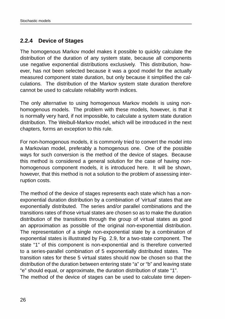
The method of the device of stages represents each state which has a non-exponential duration distribution by a combination of ‘virtual’ states that areexponentially distributed. The series and/or parallel combinations and thetransitions rates of those virtual states are chosen so as to make the durationdistribution of the transitions through the group of virtual states as goodan approximation as possible of the original non-exponential distribution.The representation of a single non-exponential state by a combination ofexponential states is illustrated by Fig. 2.9, for a two-state component. Thestate “1” of this component is non-exponential and is therefore convertedto a series-parallel combination of 5 exponentially distributed states. Thetransition rates for these 5 virtual states should now be chosen so that thedistribution of the duration between entering state “a” or “b” and leaving state“e” should equal, or approximate, the duration distribution of state “1”.The method of the device of stages can be used to calculate time depen-
26

Stochastic models
0 1
a
0
b
c d
e
Figure 2.9: Example of a device of stages
dent state probabilities, and may thus be used for addressing ageing effects,effects of preventive maintenance, or other time-dependent behaviour of thecomponent. However, it is not a solution to the problem of calculating sys-tem state duration distributions. This is best illustrated by an example. InFig. 2.10, a system with two components is depicted, each of which has twostates. Assumed is that the UP state of these components (“0” and “a”) arenegative-exponentially distributed, but the DOWN states (“1” and “b”) areWeibull distributed. The system is supposed to function when at least onecomponent is in the UP state. The question therefore is to find an expres-sion of the distribution of the system down time, which is the distribution ofthe duration of system state “1b”, which is shown in grey in Fig. 2.10.
0 a 1 a
0 b 1 b
0 a
0 b
0 a 1 a
0
1
a
b
Figure 2.10: System with two two-state components
Even for this very simple system, the expression for the system down timedistribution is not simple because it is the distribution of the minimum of aWeibull distribution with the remaining distribution of another Weibull distri-bution, for which the age is unknown.
27
Stochastic models
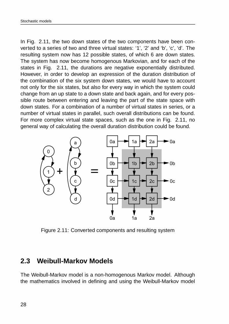
In Fig. 2.11, the two down states of the two components have been con-verted to a series of two and three virtual states: ‘1’, ‘2’ and ‘b’, ‘c’, ‘d’. Theresulting system now has 12 possible states, of which 6 are down states.The system has now become homogenous Markovian, and for each of thestates in Fig. 2.11, the durations are negative exponentially distributed.However, in order to develop an expression of the duration distribution ofthe combination of the six system down states, we would have to accountnot only for the six states, but also for every way in which the system couldchange from an up state to a down state and back again, and for every pos-sible route between entering and leaving the part of the state space withdown states. For a combination of a number of virtual states in series, or anumber of virtual states in parallel, such overall distributions can be found.For more complex virtual state spaces, such as the one in Fig. 2.11, nogeneral way of calculating the overall duration distribution could be found.
0 a 1 a 2 a
0 b 1 b 2 b
0 c 1 c 2 c
0 d 1 d 2 d
0 a
0 b
0 c
0 d
0 a 1 a 2 a
a
b
c
d
0
1
2
Figure 2.11: Converted components and resulting system
2.3 Weibull-Markov Models
The Weibull-Markov model is a non-homogenous Markov model. Althoughthe mathematics involved in defining and using the Weibull-Markov model
28

Stochastic models
are somewhat more complex than those used for the homogenous Markovmodel, it will be shown that this model lends itself for all types of reliabilitycalculations possible with the homogenous Markov model, and yet enablesa correct analytical calculation of interruption costs.
The definition of the Weibull-Markov component starts by altering the ho-mogenous component by using not a negative exponential distribution, buta Weibull distribution for the conditional state durations. The result is astochastic component, defined by
• the set of possible states � � '�� � � � �������6�� �� where � � is the numberof possible states
• the stochastic history � �$��� �! � % ��� �! � ��! � � , where
– � �! � ����� �! � � � � ����� �! � '*����� �! � � �–% ��� � ' � and � �! � % ��� �! � � � % ��� �! �
• the stochastic process�$� ����� '*����� �!
for% ��� �! � � � % ��� �! � �
• the set of continuous probability distribution functions� � ����� for the con-
ditional state durations � ��� &-,� ��� &-, ����� ' DEA � � ��� &-, � ���
' DEA � ����� �! ('*) � � % ��� � � � % ��� �! � � � � ����� � � � '0/ �' �! ����� � �
: ��� &-, � � � �����
This model with Weibull distributions, which has independent duration dis-tributions defined for each transition separately, equals the homogenousMarkov model when all shape factors
; ��� &-,equal one.
The above model is mathematically problematic in the sense that it it is evenhard to derive a useful expression for the component state duration dis-tribution. As with the homogenous model, the next state and the currentstate duration are determined by drawing outcomes for all conditional statedurations and selecting the lowest one. The probability distribution for the
29

Stochastic models
duration � ��� & of state � ��� & is therefore the distribution of the minimum of theconditional durations:� ��� & ����� ' DEA � � ��� & � ��� ' DEA � �
�:9, � � � � ��� &-, � � ���
' �! � �, � �
DEA � � ��� &-, � ��� '��! � �, � �
����� � �: ��� &-, � � � ��� �
' �! ����� �� � �, � �
�: ��� &-, � � � ������ (2.50)
Expression (2.50) can be simplified drastically by taking a same shape factorfor all conditional state durations in a same state:
; ��� &-, ' ; ��� &(2.51)
For such “same shape” models,
� ��� & ����� ' �! ����� � �: ��� & � � � � � (2.52)
�: ��� & � � � � ' �
�& � �
�: ��� &-, � � � � (2.53)
The state duration for a “same-shape” Weibull distributed component is thusagain Weibull distributed with the scale factor given by (2.53). The stochas-tic component as defined above, together with (2.51) is called a “Weibull-Markov” component.
With the expression for the state duration distribution, the transition proba-bility matrix for the Weibull-Markov component can be derived as
� � � ) � / � ' DEA � � ��� &-, '� �:9�� � � � ��� & � ���
' ����
DEA � �:9���� , � � ��� & � � ��� � ; ��� & �� � � � �
: � ��� &��� &-, ��� � ���� � ��� �� � � �' ���
�
; ��� & � � � � � �: � ��� &��� &-, ��� � ���� � � � � � �
' : ��� &: ��� &-, (2.54)
30
Stochastic models
The transition probabilities for the Weibull-Markov component are thus in-dependent of time and independent of the history of the component. TheWeibull-Markov model is thus a semi-Markov model. With the stationarytransition probabilities, it is clear that
�1��� �! is again an embedded Markov-
chain for which
DEA � ����� �! � � '0/ � ����� � ' � � ����� � '�� ������� � ����� �! .'*) �' DEA � ����� �! � � '0/ � ����� �! .'*) � ' � � � � � ) � / �
where � � � � � ) � / � is the value on the) � / position in the � ��� power of � � . For
all � � � �, � & � � , � � � � � � ) � / � '���� � .
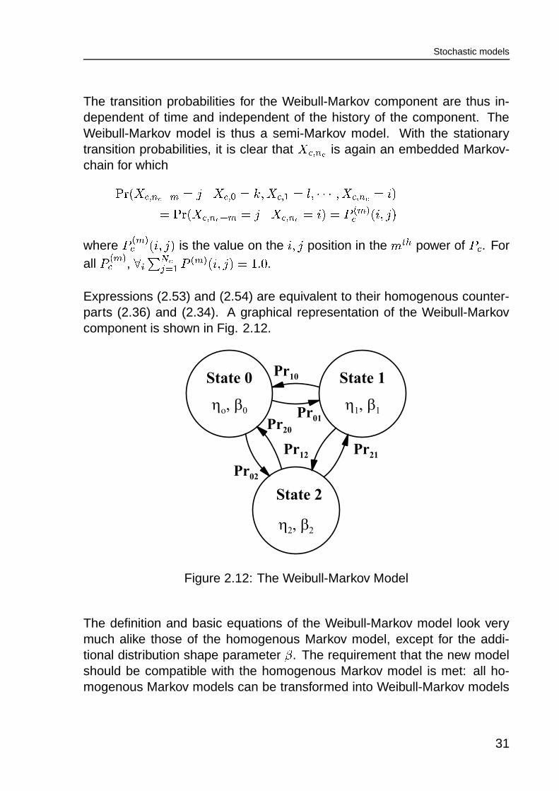
Expressions (2.53) and (2.54) are equivalent to their homogenous counter-parts (2.36) and (2.34). A graphical representation of the Weibull-Markovcomponent is shown in Fig. 2.12.
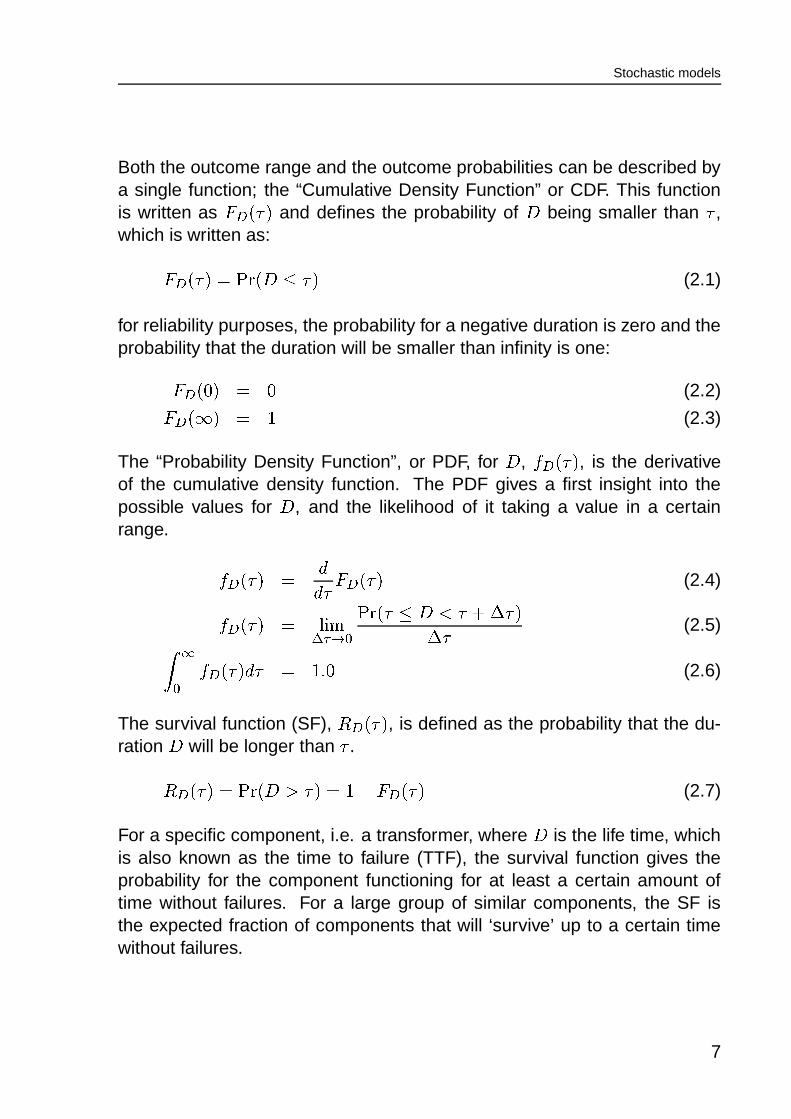
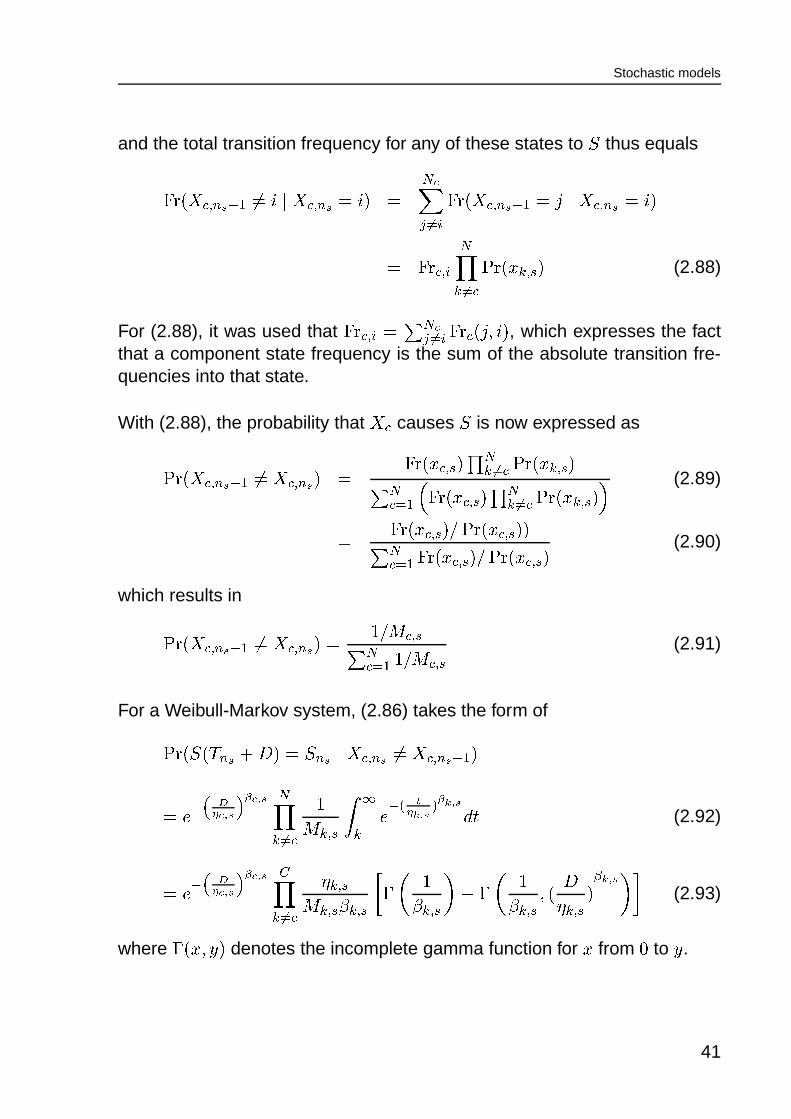
P r 0 1
P r 1 0
P r 1 2 P r 2 1
P r 2 0
P r 0 2
h o , b 0 h 1 , b 1
h 2 , b 2
S t a t e 0 S t a t e 1
S t a t e 2
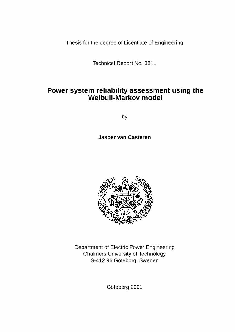
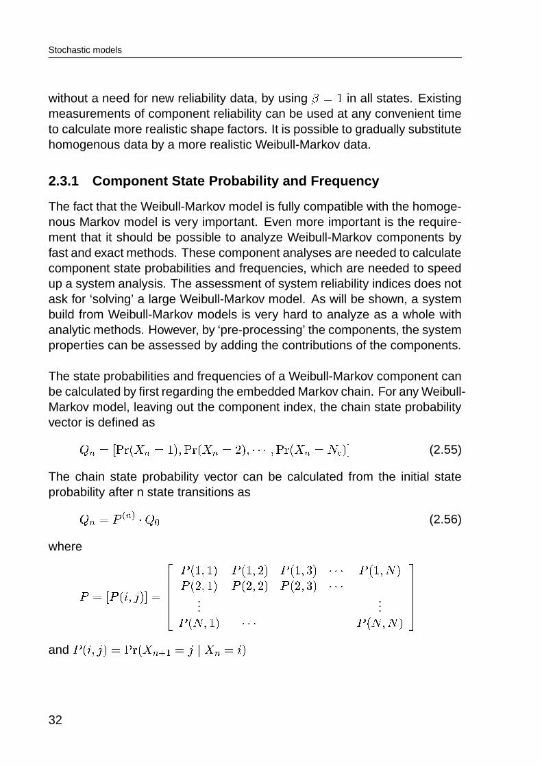
Figure 2.12: The Weibull-Markov Model
The definition and basic equations of the Weibull-Markov model look verymuch alike those of the homogenous Markov model, except for the addi-tional distribution shape parameter
;. The requirement that the new model
should be compatible with the homogenous Markov model is met: all ho-mogenous Markov models can be transformed into Weibull-Markov models
31
Stochastic models
without a need for new reliability data, by using; ' �
in all states. Existingmeasurements of component reliability can be used at any convenient timeto calculate more realistic shape factors. It is possible to gradually substitutehomogenous data by a more realistic Weibull-Markov data.
2.3.1 Component State Probability and Frequency
The fact that the Weibull-Markov model is fully compatible with the homoge-nous Markov model is very important. Even more important is the require-ment that it should be possible to analyze Weibull-Markov components byfast and exact methods. These component analyses are needed to calculatecomponent state probabilities and frequencies, which are needed to speedup a system analysis. The assessment of system reliability indices does notask for ‘solving’ a large Weibull-Markov model. As will be shown, a systembuild from Weibull-Markov models is very hard to analyze as a whole withanalytic methods. However, by ‘pre-processing’ the components, the systemproperties can be assessed by adding the contributions of the components.
The state probabilities and frequencies of a Weibull-Markov component canbe calculated by first regarding the embedded Markov chain. For any Weibull-Markov model, leaving out the component index, the chain state probabilityvector is defined as� � ' � DEA � � � '�� ��� DEA � � � ' � ��������� � DEA � � � ' � � � (2.55)
The chain state probability vector can be calculated from the initial stateprobability after n state transitions as� � ' � � � � � � (2.56)
where
� ' � � � ) � / � '������ � � � � � � � � � � � � � � � 7 � ����� � � � �� �� � � � � � � � � � � � � � � � 7 � �����
......
� � � � � � ����� � � � �� �
������
and � � ) � / � ' DEA � � � � � '0/ � � � '*) �
32

Stochastic models
In [88] it is shown that for a Markov chain with stationary transition probabil-ities, the long term state probabilities can be found by solving� ' � � � (2.57)
where� ' � � � � ��� � � � ���������6� � � � � ' ��� � � � � �(2.58)
With the Weibull-Markov component, there are no self-transitions, and there-fore � & � � � ) � ) � ' � � . The long term Markov chain state probabilities can besolved by using
� &�� � �, � � �
� ) � / � '���� ���
(2.59)
� �& � �
� � ) � '���� � (2.60)
and by taking
9 &-, ' � � � ) �� � � �if) '0/
� � ) � " � � � ) � / � if) '0/
� & ' � � ) �� ���� ' � � � � ��� � � � ��������� � � � � � �
A solution for� �
can then be found by solving
9 � ��� ' �(2.61)
and� � � � is found by using (2.60) again.
The state probabilities for the Weibull-Markov component can be calculatedfrom the embedded state probabilities as
DEA � ) � ' � � ) ��� � � � & �� �& � � � � ) ��� � � � & � (2.62)
33

Stochastic models
where� � � & � ' : & � � � � �� ��� is the expected duration of state
).
With the known Weibull-Markov state probabilitiesDEA � ) � , the state frequen-
cies@BA � ) � can be calculated as
@BA � ) � ' DEA � ) �� � � & �
2.4 The Weibull-Markov System
The Weibull-Markov system is defined in the same way as the homoge-nous Markov system; as a stochastic model of a power system for which allstochastic components are Weibull-Markov components.
The Weibull-Markov system is thus defined by
• the number of Weibull-Markov components �
• the set of Weibull-Markov components� � ����� �! � % ��� �! � ��! � � � �� � �
• the resulting stochastic system history � 2 �43 � % �43 � ��43 � � , where
–2 �43(' � � � � �43 � � � � �43 ������� � � � � �43 � and
����� �43('*��� � % �43 �– � % �43 � ��43 � � ' � �� � � � % ��� �! � �� � �
Except for the different component state duration distributions, the Weibull-Markov system behaves in the same way as the homo/-genous Markov sys-tem. Again, the probability of two components changing state at the verysame moment is zero:
���� � �� ��� � �� � % � � ��� ' % �� �� � (2.63)
and thus
� �43 � �� � �! � % �43(' % ��� �! � (2.64)
34

Stochastic models
Identical definitions for the remaining state duration and the age of the com-ponents � for all system states are used.
� � � "#5 � ' % ��� �43� � � % �43 (2.65)"#5 � ' ���� � "#� ��� � � % ��� �! � % �43
(2.66)9 � � "#5 � ' % �43 % ��� �43� (2.67)
However, where the distribution of the remaining duration of the state of a ho-mogenous component equals the distribution of the complete duration, thisis generally not the case for a Weibull-Markov component. For a Weibull-Markov component, the distribution of the remaining duration normally de-pends on the history of the system. As the system state duration is the mini-mum of the remaining component state durations, this dependency makes itvery hard, if not impossible, to derive exact expressions for the system stateduration distribution as a whole. Even more important is that also the proba-bilities for the following system state become history dependent, as they aretoo determined by the smallest outcome of the remaining component statedurations.
From this it is clear that the Weibull-Markov system is not only a non-homo/-genous model, but even not a Markov model. It will however be shown thatthe Weibull-Markov system will becomes a semi-Markov system again whenit is assumed to be stationary.
2.4.1 Weibull-Markov System State Probability and Frequency
The Weibull-Markov model can only be an alternative to the homogenousMarkov model if it is possible to calculate state probabilities and frequenciesanalytically with comparable computational efforts.
The probability for a system state7
is defined as the probability to find thesystem in that state at time � and is written as
DEA � 7 ����� ' DEA � 2 ����� ' 7 � . Forany moment in time:
� 3�5 � �
DEA � 2 ����� '87 � '��(2.68)
where � 5 is the number of possible system states.
35
Stochastic models
As all component are assumed to be statistically independent, the systemstate probability is the product of the component state probabilities:
DEA � 7 ����� '��� � �
DEA � ��� ����� ' � � � (2.69)
The frequency of a system state7
is defined as the density of the numberof transitions into the system state per unit of time, for a certain moment intime.
@BA � 7 ����� '�� ) � � � � �� � number of transitions to s in � ����� ��� ���� � (2.70)
If we write a system with only two components as2 �
, the upper index beingthe number of components, then the frequency of the system state
7 � '� ��� � ��� � at � is the frequency of
� � ����� ' ��� times the probability of� � ����� ' ��� ,
plus the frequency of� � ����� ' ��� times the probability of
� � ����� ' ��� .DEA � 7 � ����� ' DEA � ��� ����� � DEA � ��� ����� (2.71)@BA � 7 � ����� ' @BA � ��� ����� � DEA � ��� ����� � @BA � ��� ����� � DEA � ��� ����� (2.72)
This can be repeated for a third component and the two-component system:DEA � 7 � ����� ' DEA � 7 � ����� � DEA � ��� ����� (2.73)@BA � 7 � ����� ' @BA � 7 � ����� � DEA � ��� ����� � @BA � ��� ����� � DEA � 7 � ����� (2.74)
and, by induction, for the whole system:DEA � 7 ����� ' DEA � 7 � � � ����� � DEA � � � ����� (2.75)@BA � 7 ����� ' @BA � 7 � � � ����� � DEA � � � ����� � @BA � � � ����� � DEA � 7 � � � ����� (2.76)
These recursive equations for probability and frequency are independent ofthe state duration distributions. The recursive equation for the system statefrequency can be rewritten into
@BA � 7 ����� '��� � �
��@BA � � � ����� �
��� � � � � �� �
DEA � � � �������
(2.77)
or into
@BA � 7 ����� ' DEA � 7 ����� ���� � �
@BA � � � �����DEA � � � ����� (2.78)
36
Stochastic models
The equality (2.77) is known as the state frequency balance.
For the stationary system, for � � � , the component state probabilitiesand frequencies become time independent and are written as
DEA � � � � and@BA � � � � . The system state probability and frequency will then also becometime independent as
DEA � 7 � ' ��� � � �
DEA � 7 ����� '��� � �
DEA � � � � (2.79)
@BA � 7 � ' ��� � � �
@BA � 7 ������� ' DEA � 7 � ���� � �
@BA � � � �DEA � � � � (2.80)
For the stationary system, the expected state duration, or ‘state expectancy’,in units per time per unit of time, equals the state probability. The expectedsystem state duration is then calculated by dividing the system state ex-pectancy by the system state frequency:
� � � 5 � ' DEA � 7 ��� @BA � 7 � (2.81)
In most reliability assessment calculations, the unit of frequency is taken as� ��� , where � ' annum'����� � hours, and the expectancy is expressed in
hours. In that case,
� � � 5 � ' DEA � 7 � � ���� �� @BA � 7 � hours (2.82)
2.4.2 Weibull-Markov System State Duration Distribution
For homogenous systems, the system state duration distribution is foundwithout problems. Because the system too is a homogenous Markov model,the system state duration will be distributed according to a negative expo-nential distribution, with a duration rate which is the reciprocal sum of allcorresponding component transition rates.
To find an expression for the state duration distribution of a Weibull-Markovsystem, it is important that we consider stationary systems only. This meansthat all component models in the system are stationary, and the history foreach component beyond the last state change is irrelevant.
37

Stochastic models
Suppose a stationary system with two components. If we would monitorsuch a system for a short period, a graph as depicted in Fig. 2.13 could bethe result. It is now possible to regard the epochs of the one component as
1
2
A 1 (n j )
D 2 (n i ) A 2 (n i )
D 1 (n j )
n i
n j
Figure 2.13: A monitored period for a two-component system
inspection times for the other, and vice versa, as is depicted in Fig. 2.13. Aslong as each system state is treated separately, and because both compo-nents are stationary and stochastically independent, each separate epochof the one is a random inspection time for the other.
The derivation of the expression for the system state duration distributionstarts with a well known result from renewal theory, according to which acomponent
���, when found in state
)at a random inspection time � , has a
remaining state duration distribution according to
DEA � � ��� & � � � � � ��� & � ��� ' ��<��� &
� ��� � "� ��� & ����� � (2.83)
where�<��� &
is the mean duration of�$�.'*)
and� ��� & ����� ' DEA � � ��� & � ��� .
By using the random epochs of the one component as an inspection time forthe other, the remaining state duration � � � "=, � and � � � " & � in Fig. 2.13 willthus respect (2.83).
38

Stochastic models
According to (2.83), the distribution of the remaining state duration is inde-pendent of the passed state duration, � ��� & � , at the moment of inspection� , for all types of distributions for the total state duration
� ��� & ����� . From this,it follows that the probability of
� �, when found in state
)at time � , to not
change state in the interval � � � � � � � is
DEA � ��� ��� � � � '*) � ��� ����� '*) � ' ��<��� &
���� � �! "� ��� & ����� � (2.84)
Because a system will change as soon as one of its components changes,the probability of a system, consisting of � components, which is found instate
7at time � , with
% �43 � � � % �43 � � , to not change state in the interval� � � � � � � is
DEA � 2 ��� � � � '87 � 2 ����� '87 � '��� � �
�� ��� �43
���� � �! � ��� �43 ����� � (2.85)
where�<��� �43
is the mean duration of�$��� �43
and� ��� �43 ����� ' DEA � � � � �43 � ��� .
Expression (2.85) is an important first result, because it shows that it ispossible to express the remaining system state duration distribution in termsof component state properties. However, we do not want to calculate thedistribution of the remaining system state duration for arbitrary inspectiontimes, but the distribution for the whole state duration. The inspection time in(2.85) then equals the moment at which the system state starts, which is themoment at which the causing component changes its state. The distributionof the ‘remaining’ state duration for that one component will thus equal thedistribution of the total state duration. For all other components, we haveto use (2.84), as they have already spend some time in their state at themoment the new system state starts.
If we suppose that component�$�
is the causing component for system state2 �43, then it follows that he probability of that system state, when its starts at
epoch% �
because component�$�
changed state at% �
, to last longer than
39
Stochastic models
� , isDEA � 2 � % �43 � � � ' 2 �43 � ����� �43 '*����� �43 � � � '
' � �! � ��� �43 � � ������� �
�� � � �43
���� � �! � � � �43 ����� � � (2.86)
All that is left now to do is to find an expression for the probability for eachcomponent to be the causing component for system state
2 �43. Equation
(2.86) can then be weighted by that probability and the distribution of thesystem state duration can then be found by summing the weighted expres-sions for each component.
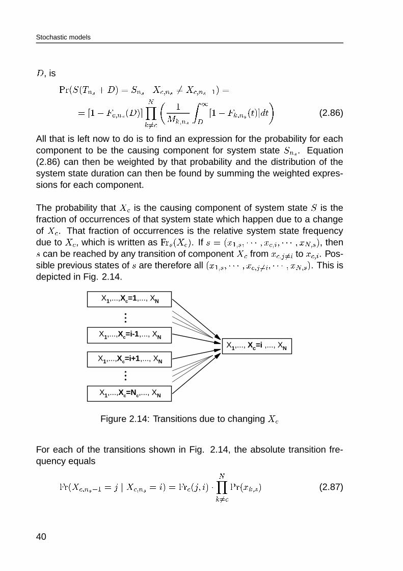
The probability that�$�
is the causing component of system state2
is thefraction of occurrences of that system state which happen due to a changeof���
. That fraction of occurrences is the relative system state frequencydue to
���, which is written as
@BAF5 � ��� � . If7 ' � ��� � 5 �������6� � ��� & ������� � � � � 5 � , then7
can be reached by any transition of component�1�
from � ��� , �� & to � ��� & . Pos-sible previous states of
7are therefore all � � � � 5 ������� � � ��� , �� & ������� � � � � 5 � . This is
depicted in Fig. 2.14.
X 1 ,..., X c =i ,..., X N
X 1 ,..., X c = 1 ,..., X N
X 1 ,..., X c = i-1 ,..., X N
X 1 ,..., X c = i+1 ,..., X N
X 1 ,..., X c = N c , ..., X N
Figure 2.14: Transitions due to changing�1�
For each of the transitions shown in Fig. 2.14, the absolute transition fre-quency equals
@BA � ����� �43 � � '0/ � ����� �43('*) � ' @BAC� � / � ) � ������� �
DEA � � � � 5 � (2.87)
40
Stochastic models
and the total transition frequency for any of these states to2
thus equals
@BA � ����� �43 � � '*) � ����� �43('*) � ' � �, �� &
@BA � ����� �43 � � '0/ � ����� �43('*) �
' @BAC��� & ������ �
DEA � � � � 5 � (2.88)
For (2.88), it was used that@BA���� &?' � � , �� & @BAC� � / � ) � , which expresses the fact
that a component state frequency is the sum of the absolute transition fre-quencies into that state.
With (2.88), the probability that�$�
causes2
is now expressed as
DEA � ����� �43 � � '*����� �43 � ' @BA � � ��� 5 � � ����� � DEA � � � � 5 �� �� � � � @BA � � ��� 5 � � ����� � DEA � � � � 5 � � (2.89)
' @BA � � ��� 5 ��� DEA � � ��� 5 ���� �� � � @BA � � ��� 5 ��� DEA � � ��� 5 � (2.90)
which results in
DEA � ����� �43 � � '*����� �43 � ' � � �<��� 5� �� � � � � �<��� 5 (2.91)
For a Weibull-Markov system, (2.86) takes the form of
DEA � 2 � % �43 � � � ' 2 �43 � ����� �43 '*����� �43 � � �
' � ������ � 3�� � � 3 ������ �
�� � � 5
���� � � ���� 3 � 3 � (2.92)
' � ������ � 3 � � � 3 ������ �
: � � 5� � � 5 ; � � 5� � �
; � � 5 � � �; � � 5 � �
�: � � 5 �� 3 ��� (2.93)
where � � � ��� � denotes the incomplete gamma function for � from � to � .
41
Stochastic models
The combination of (2.91) and (2.93) leads to the following expression forthe probability for the duration of system state
2to last longer than D:
DEA � % �43 � � % �43 � � � '��� � �
� DEA � ����� �43 � � '*����� �43 � � DEA � 2 � % �43 � � � ' 2 �43 � ����� �43 '*����� �43 � � ���
' � �� � � � ��� 5 � � ��� �<��� 5� �� � � � � �<��� 5
��� � �
����� � � � � : ��� 5 � � � 3 �� ��� 5 � � � (2.94)
where
� ��� & � � � ': ��� &; ��� & � � �
; ��� & � � � �; ��� & � �: ��� & � � � � � (2.95)
From equation 2.94 and 2.95, it is clear that the system state duration dis-tribution is independent of the previous system states in the steady statecase. The � ��� & � � � function only depends on the component state durationdistribution parameters
;and : . The � ��� & � � � values for each component can
thus be calculated prior to the actual reliability assessment.
2.5 Basic Power System Components
This chapter shows a possible implementation of a Weibull-Markov modelfor modeling stochastic power system components. The proposed methodsare introduced on the basis of a model for the synchronous generator.
2.5.1 Defining a Weibull-Markov Model
The Weibull-Markov model is determined by the following set of parameters.
• N, the number of states
• {; &
}, the set of form-factors, one for each state
• { : & }, the set of characteristic times, one for each state
• P, the transition probability matrix
42
Stochastic models
• Electrical parameters, which define the electrical model for the com-ponent for each state
It is however possible to enter the state duration parameters other than by;
and : , as in many cases, these are unknown. Alternatively,
• { � & }, the mean state durations
• { & }, the state duration variances
is possible too.
Any two of the resulting possible state duration parameters,; &
, : & , � & , & , willdetermine the other two. The following conversion formulas can be used:
� � ; � : � ' :�� � � ; �� � ; � � ' � � � ; � �� � � ; � � ; � : � ' � : � � � � ; � � ; � � � ' � � � � � ; �� � � ; �; � : � � � ' � inv� �
: �; � : � � ' � inv� �
: �; � � � � ' � inv� �
�
: � �: � ; � � � ' �� � � ; �: � ; � � ' �� � � ; �
43
Stochastic models
where� � � ; � ' + � � � � �; �� � � ; � ' � � � � �; � � � � � �
; � �
� � � ; � ' � � � ; � �� � � ; �The inversion of � � � ; � , � � � ; � and � � � ; � can be performed by newton meth-ods. De values for � � : � � , � : � � � and : � � � � can be calculated by firstcalculating the corresponding
;.
The above set of conversion formulas enables an easy definition of a Weibull-Markov model. However, it is also possible to leave all form-factors {
; &} to
their default values of one, and enter the Weibull-Markov model as a ho-mogenous Markov model. Such would be needed if no other than homoge-nous model data is available. In stead of {
; &}, { : & } and P, the homogenous
Markov model requires the input of:
• {+ &-,
}, the matrix of state transition rates
This asks for the conversion of the state transition matrix to the transitionprobability matrix P. Such conversion can be done by using (2.36).
The back transformation from the state probability matrix to a state transi-tion matrix can be performed by using the calculated state duration meansand (2.38). This back transformation makes it possible to switch between‘homogenous input mode’ and ‘Weibull-Markov input mode’, which may beused to check the validity of the model or to check the correct transformationof a homogenous model into a more realistic Weibull-Markov model.
2.5.2 A Generator Model
The basic stochastic generator model is fairly primitive, as it only definesstates for the generator being available or not available. In many applica-tions, such a two-state model is sufficient. However, there are several rea-sons to include more states to account for partial outages of the generator.Such a partial outage is a condition in which the generator is still connected
44
Stochastic models
to the net and is still producing power, but in which the maximum output islimited. Such a situation may occur when
• A run-of-the-river hydro turbine is reduced in capacity due to a low riverlevel.
• A large, multi-machine thermal power plant is reduced in capacity dueto the outage of one or more generator units.
• The available power is reduced due to the outage of a sub-component,such as a pulverizer, a fan, a feed water or cooling water pump, etc.
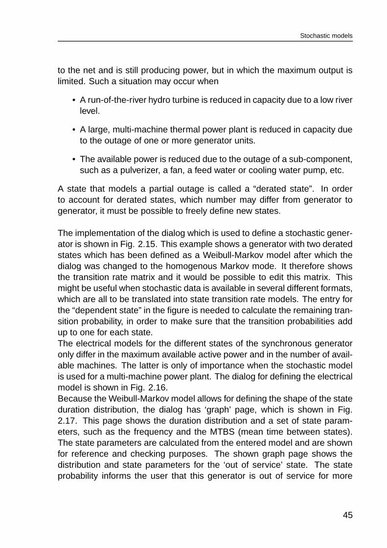
A state that models a partial outage is called a “derated state”. In orderto account for derated states, which number may differ from generator togenerator, it must be possible to freely define new states.
The implementation of the dialog which is used to define a stochastic gener-ator is shown in Fig. 2.15. This example shows a generator with two deratedstates which has been defined as a Weibull-Markov model after which thedialog was changed to the homogenous Markov mode. It therefore showsthe transition rate matrix and it would be possible to edit this matrix. Thismight be useful when stochastic data is available in several different formats,which are all to be translated into state transition rate models. The entry forthe “dependent state” in the figure is needed to calculate the remaining tran-sition probability, in order to make sure that the transition probabilities addup to one for each state.The electrical models for the different states of the synchronous generatoronly differ in the maximum available active power and in the number of avail-able machines. The latter is only of importance when the stochastic modelis used for a multi-machine power plant. The dialog for defining the electricalmodel is shown in Fig. 2.16.Because the Weibull-Markov model allows for defining the shape of the stateduration distribution, the dialog has ‘graph’ page, which is shown in Fig.2.17. This page shows the duration distribution and a set of state param-eters, such as the frequency and the MTBS (mean time between states).The state parameters are calculated from the entered model and are shownfor reference and checking purposes. The shown graph page shows thedistribution and state parameters for the ‘out of service’ state. The stateprobability informs the user that this generator is out of service for more
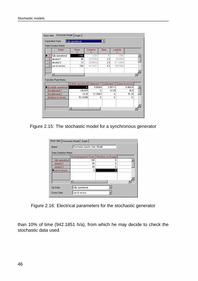
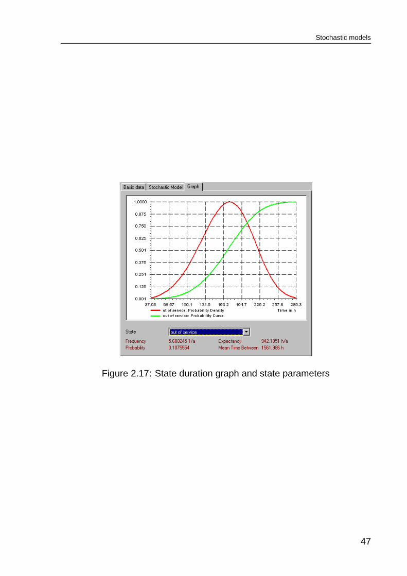
45
Stochastic models
Figure 2.15: The stochastic model for a synchronous generator
Figure 2.16: Electrical parameters for the stochastic generator
than 10% of time (942.1851 h/a), from which he may decide to check thestochastic data used.
46
Stochastic models
Figure 2.17: State duration graph and state parameters
47

Chapter 3
Applications / Examples
3.1 Comparison with Monte Carlo Simulation
The methods presented in this thesis for calculating the system state du-ration distribution by evaluating (2.94) and (2.95) were tested for a smallsystem of 20 two-state components. As the test system was strictly ‘(n-1)’,two or more overlapping outages were taken to result in an interruption.
Two cases were analyzed: one with; ' ��� � for the repair duration distri-
bution, which thus resulted in a homogenous Markov system, and one with; ' 7 � � , thus modeling a bell-shaped repair duration distribution. In bothcases, the lifetime distribution was modeled with
; ' �and the mean repair
duration was set to 5. All components used the same stochastic data inorder to make hand-calculated checks possible.
Both a Monte Carlo simulation and a state enumeration method were usedto find the interruption duration distribution for both cases. The four resultingdistribution functions (
DEA � ��� )) are shown in Fig. 3.1.This result shows a close resemblance between the Monte-Carlo result andthe analytical result. The distribution for
; ' �is, as can be shown easily,
close to the exponential distribution with a scale factor equal to half the meanrepair duration. Differences between the two curves are not due to an errorin the analytic (Weibull-Markov) model. In stead, they are caused by theinaccuracy in the Monte-Carlo simulation.
48

Applications / Examples
0
0.2
0.4
0.6
0.8
1
0 2 4 6 8 10duration
Monte-Carlo, beta=3Analytic, beta=3
Monte-Carlo, beta=1Analytic, beta=1
Figure 3.1: Calculated Duration Distribution Functions
3.2 Small System Example
To demonstrate both the use and the importance of the Weibull-Markovmodel, a small example system has been analyzed. A single line diagram ofthis example system is depicted in Fig. 3.2. The boxed data shows the linefailure frequency and expected down time per year. This data was enteredas per length values. The complete set of reliability data is listed in Table3.1. Both the lifetime and the repair duration are negative exponentially dis-tributed, as
; � '��and
; � '��.
line length failure rate; � repair duration
; �km 1/a � � ��� � � h
L1 10 1 1 2 1L2ab 30 2 1 2.5 1L3 3 3 1 1.5 1
Table 3.1: Line data used
The load point data used is listed in Table 3.2. All three loads use the same
49
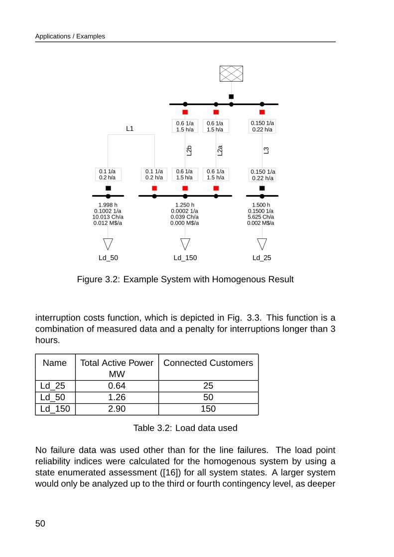
Applications / Examples
L1
0.1 1/a 0.2 h/a
0.1 1/a 0.2 h/a
L2b
0.6 1/a 1.5 h/a
0.6 1/a 1.5 h/a
L3
Ld_25
1.500 h 0.1500 1/a 5.625 Ch/a 0.002 M$/a
Ld_150
1.250 h 0.0002 1/a 0.039 Ch/a 0.000 M$/a
Ld_50
1.998 h 0.1002 1/a
10.013 Ch/a 0.012 M$/a
L2a
0.6 1/a 1.5 h/a
0.6 1/a 1.5 h/a
0.150 1/a 0.22 h/a
0.150 1/a 0.22 h/a
Figure 3.2: Example System with Homogenous Result
interruption costs function, which is depicted in Fig. 3.3. This function is acombination of measured data and a penalty for interruptions longer than 3hours.
Name Total Active Power Connected CustomersMW
Ld_25 0.64 25Ld_50 1.26 50Ld_150 2.90 150
Table 3.2: Load data used
No failure data was used other than for the line failures. The load pointreliability indices were calculated for the homogenous system by using astate enumerated assessment ([16]) for all system states. A larger systemwould only be analyzed up to the third or fourth contingency level, as deeper
50
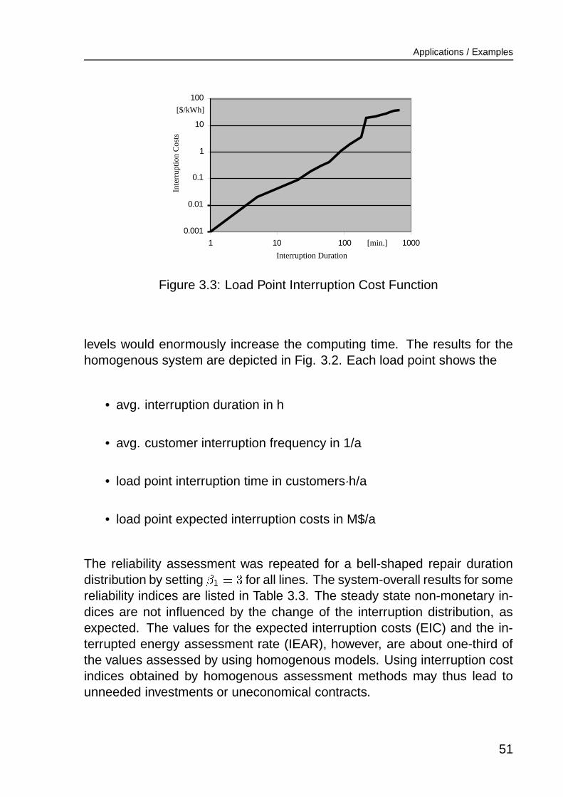
Applications / Examples
0.001
0.01
0.1
1
10
100
1 10 100 1000
Interruption Duration
[min.]
Inte
rrup
tion
Cos
ts
[$/kWh]
Figure 3.3: Load Point Interruption Cost Function
levels would enormously increase the computing time. The results for thehomogenous system are depicted in Fig. 3.2. Each load point shows the
• avg. interruption duration in h
• avg. customer interruption frequency in 1/a
• load point interruption time in customers � h/a
• load point expected interruption costs in M$/a
The reliability assessment was repeated for a bell-shaped repair durationdistribution by setting
; � '87for all lines. The system-overall results for some
reliability indices are listed in Table 3.3. The steady state non-monetary in-dices are not influenced by the change of the interruption distribution, asexpected. The values for the expected interruption costs (EIC) and the in-terrupted energy assessment rate (IEAR), however, are about one-third ofthe values assessed by using homogenous models. Using interruption costindices obtained by homogenous assessment methods may thus lead tounneeded investments or uneconomical contracts.
51
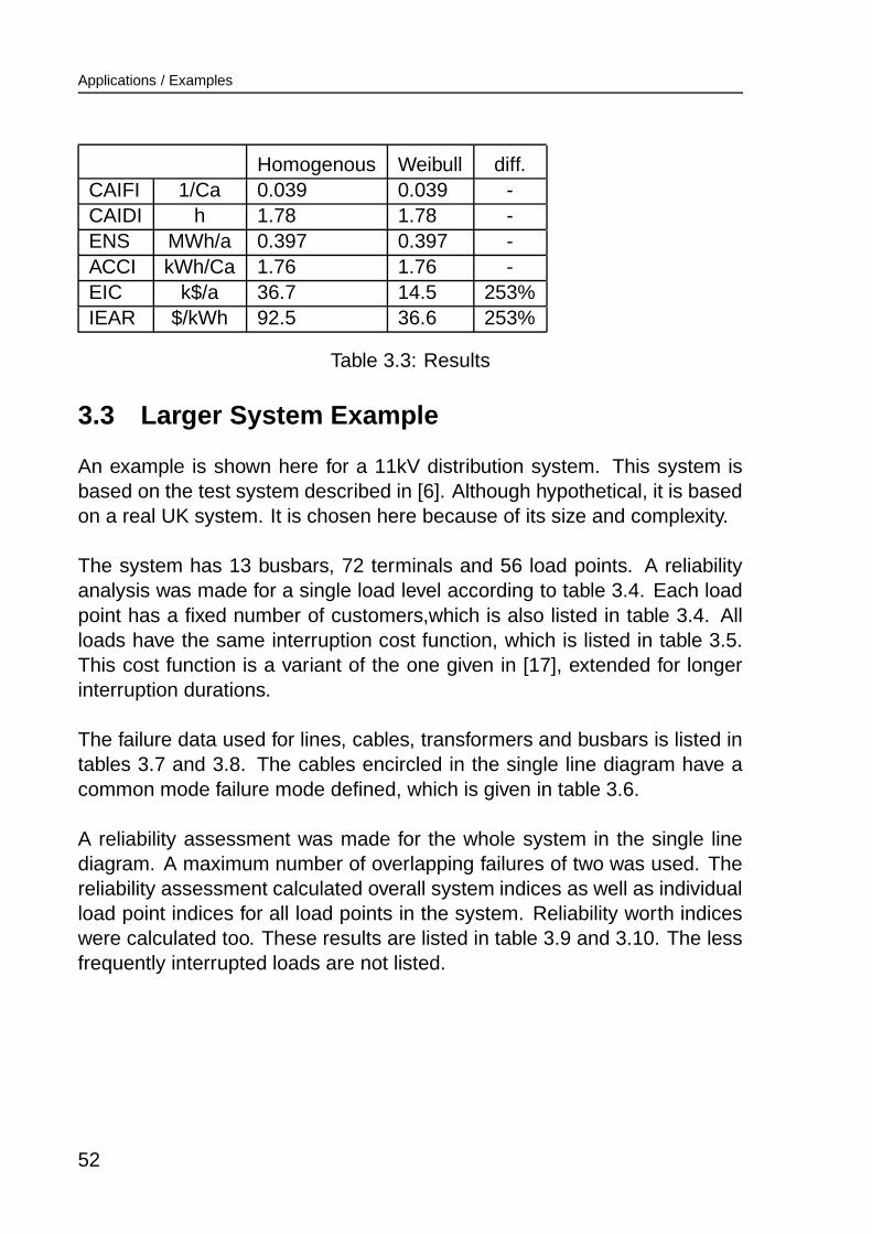
Applications / Examples
Homogenous Weibull diff.CAIFI 1/Ca 0.039 0.039 -CAIDI h 1.78 1.78 -ENS MWh/a 0.397 0.397 -ACCI kWh/Ca 1.76 1.76 -EIC k$/a 36.7 14.5 253%IEAR $/kWh 92.5 36.6 253%
Table 3.3: Results
3.3 Larger System Example
An example is shown here for a 11kV distribution system. This system isbased on the test system described in [6]. Although hypothetical, it is basedon a real UK system. It is chosen here because of its size and complexity.
The system has 13 busbars, 72 terminals and 56 load points. A reliabilityanalysis was made for a single load level according to table 3.4. Each loadpoint has a fixed number of customers,which is also listed in table 3.4. Allloads have the same interruption cost function, which is listed in table 3.5.This cost function is a variant of the one given in [17], extended for longerinterruption durations.
The failure data used for lines, cables, transformers and busbars is listed intables 3.7 and 3.8. The cables encircled in the single line diagram have acommon mode failure mode defined, which is given in table 3.6.
A reliability assessment was made for the whole system in the single linediagram. A maximum number of overlapping failures of two was used. Thereliability assessment calculated overall system indices as well as individualload point indices for all load points in the system. Reliability worth indiceswere calculated too. These results are listed in table 3.9 and 3.10. The lessfrequently interrupted loads are not listed.
52
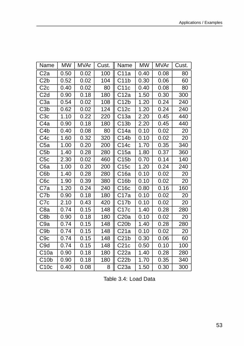
Applications / Examples
Name MW MVAr Cust. Name MW MVAr Cust.
C2a 0.50 0.02 100 C11a 0.40 0.08 80C2b 0.52 0.02 104 C11b 0.30 0.06 60C2c 0.40 0.02 80 C11c 0.40 0.08 80C2d 0.90 0.18 180 C12a 1.50 0.30 300C3a 0.54 0.02 108 C12b 1.20 0.24 240C3b 0.62 0.02 124 C12c 1.20 0.24 240C3c 1.10 0.22 220 C13a 2.20 0.45 440C4a 0.90 0.18 180 C13b 2.20 0.45 440C4b 0.40 0.08 80 C14a 0.10 0.02 20C4c 1.60 0.32 320 C14b 0.10 0.02 20C5a 1.00 0.20 200 C14c 1.70 0.35 340C5b 1.40 0.28 280 C15a 1.80 0.37 360C5c 2.30 0.02 460 C15b 0.70 0.14 140C6a 1.00 0.20 200 C15c 1.20 0.24 240C6b 1.40 0.28 280 C16a 0.10 0.02 20C6c 1.90 0.39 380 C16b 0.10 0.02 20C7a 1.20 0.24 240 C16c 0.80 0.16 160C7b 0.90 0.18 180 C17a 0.10 0.02 20C7c 2.10 0.43 420 C17b 0.10 0.02 20C8a 0.74 0.15 148 C17c 1.40 0.28 280C8b 0.90 0.18 180 C20a 0.10 0.02 20C9a 0.74 0.15 148 C20b 1.40 0.28 280C9b 0.74 0.15 148 C21a 0.10 0.02 20C9c 0.74 0.15 148 C21b 0.30 0.06 60C9d 0.74 0.15 148 C21c 0.50 0.10 100C10a 0.90 0.18 180 C22a 1.40 0.28 280C10b 0.90 0.18 180 C22b 1.70 0.35 340C10c 0.40 0.08 8 C23a 1.50 0.30 300
Table 3.4: Load Data
53
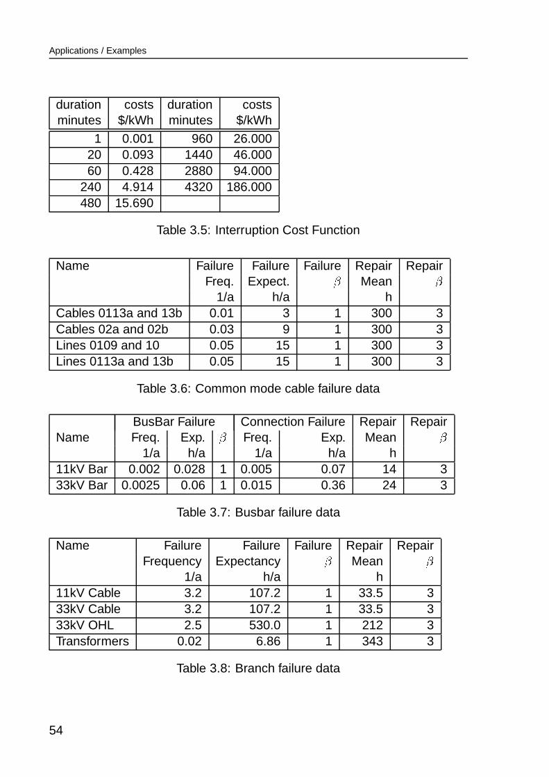
Applications / Examples
duration costs duration costsminutes $/kWh minutes $/kWh
1 0.001 960 26.00020 0.093 1440 46.00060 0.428 2880 94.000
240 4.914 4320 186.000480 15.690
Table 3.5: Interruption Cost Function
Name Failure Failure Failure Repair RepairFreq. Expect.
;Mean
;1/a h/a h
Cables 0113a and 13b 0.01 3 1 300 3Cables 02a and 02b 0.03 9 1 300 3Lines 0109 and 10 0.05 15 1 300 3Lines 0113a and 13b 0.05 15 1 300 3
Table 3.6: Common mode cable failure data
BusBar Failure Connection Failure Repair RepairName Freq. Exp.
;Freq. Exp. Mean
;1/a h/a 1/a h/a h
11kV Bar 0.002 0.028 1 0.005 0.07 14 333kV Bar 0.0025 0.06 1 0.015 0.36 24 3
Table 3.7: Busbar failure data
Name Failure Failure Failure Repair RepairFrequency Expectancy
;Mean
;1/a h/a h
11kV Cable 3.2 107.2 1 33.5 333kV Cable 3.2 107.2 1 33.5 333kV OHL 2.5 530.0 1 212 3Transformers 0.02 6.86 1 343 3
Table 3.8: Branch failure data
54

Applications / Examples
State Enumeration AnalysisSystem SummaryCustomer Avg. Interruption Freq. Index CAIFI 0.08 1/CaCustomer Avg. Interruption Duration Index CAIDI 7.1 hAvg. Service Unavailability Index ASUI 0.000068Expected Energy Not Supplied ENS 31 MWh/aAvg. Customer Curtailment Index ACCI 0.003 MWh/CaExpected Interruption Cost EIC 0.036 M$/aInterrupted Energy Assessment Rate IEAR 1.2 $/kWh
Table 3.9: Overall system reliability indices
State Enumeration AnalysisLoad Point InterruptionsName LPIT LPIF AID LPENS LPEIC ACIF ACIT
Ch/a C/a h MWh/a k$/a 1/a h/a
C13a 440.67 60.58 7.27 2.20 2.54 0.14 1.00C23a 356.70 32.15 11.09 1.78 2.24 0.11 1.19C14c 331.71 43.51 7.62 1.66 1.83 0.13 0.98C10a 284.19 15.97 17.79 1.42 1.87 0.09 1.58C5c 261.28 22.19 11.77 1.31 1.70 0.05 0.57C15a 256.51 21.58 11.89 1.28 1.70 0.06 0.71C7c 256.00 36.60 7.00 1.28 1.59 0.09 0.61C22a 231.10 18.89 12.23 1.16 1.55 0.07 0.83C6c 217.13 33.11 6.56 1.09 1.41 0.09 0.57C4c 185.22 27.88 6.64 0.93 1.19 0.09 0.58C10b 180.85 19.37 9.34 0.90 1.09 0.11 1.00C9b 179.72 18.63 9.65 0.90 1.11 0.13 1.21c9c 179.72 18.63 9.65 0.90 1.11 0.13 1.21c9d 179.72 18.63 9.65 0.90 1.11 0.13 1.21C12a 178.32 35.28 5.05 0.89 0.90 0.12 0.59C7a 166.75 29.18 5.71 0.83 0.94 0.12 0.69C3c 151.54 12.26 12.36 0.76 0.83 0.06 0.69C13b 146.30 19.07 7.67 0.73 0.84 0.04 0.33C17c 134.96 15.89 8.49 0.67 0.85 0.06 0.48C15c 133.56 29.21 4.57 0.67 0.74 0.12 0.56
55

Applications / Examples
State Enumeration AnalysisLoad Point Interruptions, continuedName LPIT LPIF AID LPENS LPEIC ACIF ACIT
Ch/a C/a h MWh/a k$/a 1/a h/a
C20b 129.12 38.63 3.34 0.65 0.58 0.14 0.46C10c 122.72 8.59 14.29 0.61 0.78 0.11 1.53C9a 120.36 18.66 6.45 0.60 0.68 0.13 0.81C2b 113.12 7.96 14.22 0.57 0.68 0.08 1.09C5a 112.59 8.64 13.03 0.56 0.74 0.04 0.56C6a 112.49 13.52 8.32 0.56 0.74 0.07 0.56C2a 108.76 7.65 14.22 0.54 0.66 0.08 1.09C4a 100.58 8.68 11.58 0.50 0.67 0.05 0.56C8b 92.05 9.46 9.73 0.46 0.55 0.05 0.51C3a 80.96 8.29 9.77 0.40 0.41 0.08 0.75C16c 73.74 9.08 8.12 0.37 0.48 0.06 0.46C12c 61.88 25.85 2.39 0.31 0.15 0.11 0.26C12b 53.36 28.27 1.89 0.27 0.06 0.12 0.22C2d 45.63 7.87 5.80 0.23 0.18 0.04 0.25C15b 45.11 17.06 2.64 0.23 0.20 0.12 0.32C11a 43.05 4.80 8.97 0.22 0.23 0.06 0.54C21c 34.68 5.59 6.21 0.17 0.19 0.06 0.35C3b 34.60 9.55 3.62 0.17 0.02 0.08 0.28C7b 33.12 21.93 1.51 0.17 0.05 0.12 0.18C11b 32.28 3.60 8.97 0.16 0.17 0.06 0.54C8a 31.27 18.71 1.67 0.16 0.03 0.13 0.21C11c 24.51 4.81 5.09 0.12 0.08 0.06 0.31C22b 23.37 13.73 1.70 0.12 0.03 0.04 0.07C21b 21.49 3.35 6.41 0.11 0.12 0.06 0.36C16a 21.43 0.64 33.49 0.11 0.15 0.03 1.07C17a 21.43 0.64 33.49 0.11 0.15 0.03 1.07C2c 19.08 6.16 3.10 0.10 0.01 0.08 0.24C5b 12.20 12.18 1.00 0.06 0.01 0.04 0.04C21a 10.71 0.32 33.49 0.05 0.07 0.02 0.54C20a 10.71 0.32 33.49 0.05 0.07 0.02 0.54
Table 3.10: Load point reliability indices
56
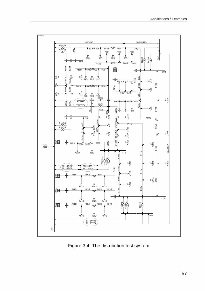
Applications / Examples
DIgSILENT
B09
B07
B04
B01
B13
B11
B12
B02
B08
B05
S16a S16b S16c S16d
S17a S17dS17cS17b
S15a
S15b
S15c
S15d
S14aS14d
S14b S14c
S20a S20b S20c S20d
S02a
S02e S02fS02b S02c S02d
S10c
S10a
S10b
S10d
S10e
S11a
S11b
S11c
S11d
S12a
S12b
S12d
S12c
S05c
S05d
S05a
S05b
S22c
S22d
S22a
S22b
S04c S04dS04a S04b
S07a
S07b
S07c
S07d
S21b
S21a
S21d
S21c
S03a S03b S03c S03d
S08a
S08b
S08e
S08c
S08d
S09d S09c S09b S09a
S23a
S23b
S06a S06b S06c S06d
S13a
S13b
S13c
Cable0110
C21bC21a C21c
C7b
C7a
C7c
C2c
C3b
C2b
C3a
Cable0109
C2d
C3c
C22
bC22
a
C4cC4a
C6a C6c
C5b
C5c
C5a
C13
aC13
b
C20a C20b
Cable06t06
ES4
Cab0113aCab0113b
ES3
ES5
C16a
ES8
C16b C16c
C17a C17cC17b
T01
13b
Line0113a
T01
13a
Line0113b
ES7
T0102b
T0102a
Line09
07
T07
08
T06
08
Linet0601
C2a
T0405
T0305
Cable02a
Cable02b
C14a C14cC14b
C10
b
C9a
T09
11
T1201a
T1201b
C4b
C6b
T10
11a
ES2
C15
bC15
aC15
cC12
aC12
bC12
cC23
a
T10
11b
C11
bC11
aC11
c
C10
aC10
c
C8b
C8a
c9d c9c C9b
Figure 3.4: The distribution test system
57
Chapter 4
Conclusions
The Weibull-Markov stochastic model that is introduced in this LicenciateThesis is 100% compatible with the widely used homogenous Markov model.It enables all necessary analytic calculations on the component level, includ-ing the calculation of the component state frequencies and probabilities.
A system that is build from Weibull-Markov components is not a Markovmodel but the stationary system again becomes a semi-Markov model. Thecalculation of system state probabilities and frequencies can also be per-formed when the system is not stationary, by combining the contributions ofthe components, and does not require the solving of large matrix equations.
An expression has been found for the system state duration distributions.This expressions allows for a fast assessment of interruption costs duringa state enumerated reliability assessment. Such costs assessment are notpossible with the homogenous Markov model.
At this point in research, it is believed that all reliability assessment methodsthat have been developed for the homogenous Markov model can also beused in combination with the Weibull-Markov model. The Weibull-Markovmodels is therefore a good alternative to the homogenous Markov model.
58

Appendix A
Glossary of Terms
Stochastic power system component. A power system component is saidto be stochastic when it has a countable set of functional states inwhich it may reside, and when the time spend in a state, and the (num-ber of the) next state are both stochastic quantities.
Stochastic component behavior. The stochastic behavior of a componentis the description of the way in which the component changes from onestate to another. This includes
• all the possible transitions from one state to another
• a description of the stochastic durations for each possible state
• the probabilities for the transitions to other states, given the cur-rent state.
Component A component is a typical part of the electric power systemwhich is treated as one single object in the reliability analysis. Ex-amples are a specific switch, transformer, line, generator, etc. Com-ponent may reside in different states, such as ’being available’, ’beingrepaired’, etc.
System A ‘system’ is short for an electrical power system. A system isbuild from components and changes state when one of its componentschanges state. The resulting ’system state’ is the combination of allcomponent states.
Event An event is a transition of a component between its states.
59

Glossary of Terms
Outage An component outage is defined as the situation in which the com-ponent cannot be used, either because it has been taken out of ser-vice deliberately (‘planned’ outage), either because it has failed (‘un-planned’, or ‘forced’, outage).
Healthy State A healthy system state is a situation in which no unplannedoutages are present.
Contingency A contingency is a system state in which one or more un-planned outages are present.
Coherent System Also called “consistent system”. A system in which ad-ditional outages will never improve the system performance.
Active Failure A failure of a component which activates the automatic pro-tection system. Active failures are normally associated with short-circuits.
Adequacy The ability of the electrical power system to meet the load de-mands under various steady state system conditions.
Availability The fraction of time a component is able to operate as intended,either expressed as real fraction, or as hours per year.
Base State A system state in which no failures or outages are present.
Contingency A system state in which one or more unplanned outages arepresent.
Distribution Function The distribution function for the stochastic quantityX equals the cumulative density function CDF(x).
CDF(x) = the probability of X to take a value smaller than x.
Failure A failure is an undesirable event of a component.
Failure Effect Analysis (FEA) The electrical steady state and/or dynamicanalysis of the system, possibly combined with switching, generatorrescheduling, or other alleviation techniques, in order to assess thenumber of loads which would have to be curtailed.
60

Glossary of Terms
Hazard Rate Function The function HRF(x), describing the probability ofa stochastic quantity to be larger than x+dx, given the fact that it islarger than x, divided by dx. The hazard rate may thus describe theprobability of a element to fail in the next period of time, given thefact that it is still functioning properly. The hazard rate is often usedto describe ageing and wear out. A famous example is the so-called“bath-tub” function which describes the probability of a device to fail inthe next period of time during wear-in, normal service time and wear-out.
Hidden Failure An event of a component which will prevent it from operat-ing as intended the next time will be called upon.
Interruption An unplanned zero-voltage situation at one or more load pointsdue to outages in the system.
Maintenance The planned removal of one or more primary componentsfrom the system.
(n-1) system A system for which all relevant components are redundantunits.
(n-k) system A system for which the outage of any k components will neverlead to an interruption in the base state.
Outage The removal of a primary component from the system.
Passive Failure A failure of a component which does not activate the auto-matic protection system.
Probability Density Function The function PDF(x), describing the proba-bility of the stochastic quantity to take a value from an interval aroundx, divided by the length of that interval. The PDF(x) is the derivative ofthe CDF(x).
Redundant Unit A component which outage will never lead to an interrup-tion in the base state, but for which at least one contingency stateexists for which its additional outage will lead to an interruption.
Repair The restoration of the functionality of a component, either by replac-ing the component or by repairing it.
61
Glossary of Terms
Scheduled Outage The planned removal of a primary component from thesystem, i.e. for preventive maintenance.
Security The ability of the system to meet the loads demands during andafter a transient or dynamic disturbance of the system.
Spare Unit A reserve component, not connected to the system, which maybe used as a replacement for a component on outage by switching orreplacing.
Statistic Statistic calculation methods are used to analyze stochastic quan-tities. A simple example is the method for calculating a mean repairduration by dividing the total time spend repairing by the number ofrepairs performed.
Information obtained by using statistic tools on measured data can beused to build stochastic models of the observed equipment.
Stochastic A quantity is said to be stochastic when its value is random andthus unknown. The range of possible values, however, may be knownas well as the likelihood of these possible values. The number of eyesthrown with a dice is random, the possible outcomes are {1,2,3,4,5,6}and the likelihood is
�
� for each outcome. For a continuous range ofpossible outcomes, the likelihood is a continuous function, known asthe Probability Density Function or “PDF”.
62
Bibliography
[1] Prof. R.N. Allan and Dr. M.H.J. Bollen. Reliability assessment of powersystems. UMIST dep. of Electr. Engineering and Electronics, 1996.lecture notes, MSc course, module 107.
[2] R.N. Allan, R. Billinton, A.M. Breipohl, and C.H. Grigg. Bibliography onthe application of probability methods in power system reliability eval-uation : 1987 - 1991. IEEE transactions on Power Systems, 9(1):41,1994.
[3] R.N. Allan, R. Billinton, and S.H. Lee. Bibliography on the appli-cation of probability methods in power system reliability evaluation :1977 - 1982. IEEE transactions on Power Apparatus and Systems,103(2):275, 1984.
[4] R.N. Allan, R. Billinton, S.M. Shahidehpour, and C. Singh. Bibliogra-phy on the application of probability methods in power system relia-bility evaluation : 1982 - 1987. IEEE transactions on Power Systems,3(4):1555, 1988.
[5] R.N. Allan and M.G. da Silva. Evaluation of reliability indices and out-age costs in distribution systems. IEEE transactions on Power Sys-tems, 10(1):413, 1995.
[6] R.N. Allan, E.N. Dialynas, and I.R. Homer. Modelling and evaluat-ing the reliability of distribution systems. IEEE transactions on PowerApparatus and Systems, 98:2181–2189, 1979.
[7] Richard E. Barlow and Frank Proschan. Statistical theory of reliabilityand life testing. Probability models. Holt, Rinehart and Winston, inc.,1975.
63

Glossary of Terms
[8] I. Bazovsky. Reliability Theory and Practice. Prentice Hall, N.J., 1961.
[9] Lina Bertling. On reliability assessment of distribution systems andreliability centered maintenance. Master’s thesis, Royal Institute ofTechnology, Stockholm, 1999.
[10] M.R. Bhuiyan and R.N. Allan. Modelling multistate problems in se-quential simulation of power system reliability studies. IEE Proc.-Gener. Transm. Distrib., 142(4):343, 1995.
[11] R. Billinton. Bibliography on the application of probability methods inpower system reliability evaluation : .. - 1971. IEEE transactions onPower Apparatus and Systems, 93:649, 1970.
[12] R. Billinton and W. Li. Hybrid approach for reliability evaluation of com-posite generation and transmission systems using monte-carlo simu-lation and enumeration techniques. IEE proceedings-C, 138(3):233,1991.
[13] R. Billinton and J. Satish. Reliability cost/reliability worth assessmentof station configurations. In IEEE WESCANEX 95, pages 175–80,New York, 1995. IEEE.
[14] R. Billinton and W. Zhang. Enhanced adequacy equivalent for com-posite power system reliability. IEE Proc.-Gener. Transm. Distrib.,143(5):420, 1996.
[15] Roy Billinton. Power System Reliability Evaluation. Gordon andBreach, 1970.
[16] Roy Billinton and Roland N. Allan. Reliability evaluation of power sys-tems. Pitman publishing, 1984.
[17] Roy Billinton and Wenyuan Li. Reliability assessment of electric powersystems using Monte Carlo methods. Plenum Press, New York, 1994.
[18] Roy Billinton and Guangbin Lian. Effect of dependent outages oncomposite system reliability performance. IEEE WESCANEX 93.Communications, Computers and Power in the Modern EnvironmentConference Proceedings, pages 127–33, 1993.
64
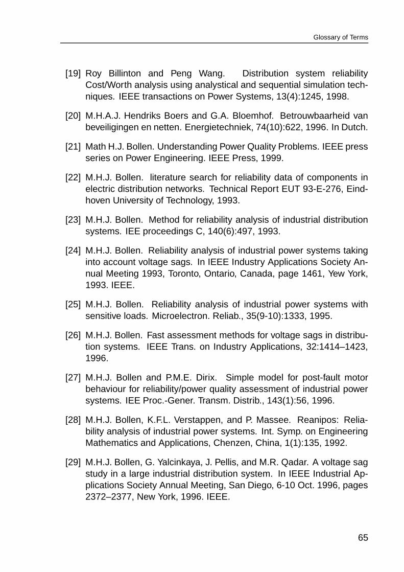
Glossary of Terms
[19] Roy Billinton and Peng Wang. Distribution system reliabilityCost/Worth analysis using analystical and sequential simulation tech-niques. IEEE transactions on Power Systems, 13(4):1245, 1998.
[20] M.H.A.J. Hendriks Boers and G.A. Bloemhof. Betrouwbaarheid vanbeveiligingen en netten. Energietechniek, 74(10):622, 1996. In Dutch.
[21] Math H.J. Bollen. Understanding Power Quality Problems. IEEE pressseries on Power Engineering. IEEE Press, 1999.
[22] M.H.J. Bollen. literature search for reliability data of components inelectric distribution networks. Technical Report EUT 93-E-276, Eind-hoven University of Technology, 1993.
[23] M.H.J. Bollen. Method for reliability analysis of industrial distributionsystems. IEE proceedings C, 140(6):497, 1993.
[24] M.H.J. Bollen. Reliability analysis of industrial power systems takinginto account voltage sags. In IEEE Industry Applications Society An-nual Meeting 1993, Toronto, Ontario, Canada, page 1461, Yew York,1993. IEEE.
[25] M.H.J. Bollen. Reliability analysis of industrial power systems withsensitive loads. Microelectron. Reliab., 35(9-10):1333, 1995.
[26] M.H.J. Bollen. Fast assessment methods for voltage sags in distribu-tion systems. IEEE Trans. on Industry Applications, 32:1414–1423,1996.
[27] M.H.J. Bollen and P.M.E. Dirix. Simple model for post-fault motorbehaviour for reliability/power quality assessment of industrial powersystems. IEE Proc.-Gener. Transm. Distrib., 143(1):56, 1996.
[28] M.H.J. Bollen, K.F.L. Verstappen, and P. Massee. Reanipos: Relia-bility analysis of industrial power systems. Int. Symp. on EngineeringMathematics and Applications, Chenzen, China, 1(1):135, 1992.
[29] M.H.J. Bollen, G. Yalcinkaya, J. Pellis, and M.R. Qadar. A voltage sagstudy in a large industrial distribution system. In IEEE Industrial Ap-plications Society Annual Meeting, San Diego, 6-10 Oct. 1996, pages2372–2377, New York, 1996. IEEE.
65
Glossary of Terms
[30] Walter F. Bückner, Rolf Eitle, and Erich Klingert. Lebensdauer der frei-leitungsseile - betriebskontrolle, produkthaftung, risikovorsorge. Elek-trizitätswirtschaft, 97(23):42, 1998. in German.
[31] L.E. Conrad (chair). Proposed chapter 9 for predicting voltage sags(dips) in revision to ieee std.493. IEEE Trans. on Industry Applications,30:805–821, 1994.
[32] A.A. Chowdhury and Don O. Koval. Value-Based power system re-liability planning. IEEE trans. on Industry Applications, 35:305–311,1999.
[33] D.P. Clancy and G. Gross. Probabilistic flows for reliability evaluationof multiarea power system interconnections. Electrical power & en-ergy systems, 5(2):101, 1983.
[34] R.D. Damstra and P. Wijdenes. De praktijk van risicobeheersing. En-ergietechniek, 75:247, april 1997.
[35] G. Douard and L. Feltin. Reliability assessment tools: EDF’s experi-ence and projects. PMAPS 4th conference, page 287, 1994.
[36] J. Endrenyi. Reliability Modeling in Electric Power Systems. JohnWiley & Sons, 1978.
[37] D.O. Kopval et.al. IEEE Recommended Practice for the Design ofReliable Industrial and Commercial Power Systems. IEEE Inc., NewYork, 1998. IEEE Std 493-1997.
[38] Nippert et.al. Zur aussagekraft der ergebnisse von zuverlässigkeits-berechnungen. Elektrizitätswirtschaft, 16(16):30, 1998. in German.
[39] Roger C. Dugan et.al. Electrical Power Systems Quality. McGraw-Hill,1996.
[40] R.N. Fontoura Filho, M.Th. Schilling, and J.L.R.Pereira. Power systeminterconnection reliability assessment by using adequacy equivalents.PMAPS 4th conference, page 323, 1994.
[41] IEEE Reliability Test System Task Force. IEEE reliability test system.IEEE transactions on Power Apparatus and Systems, 98(6):2047,1979.
66
Glossary of Terms
[42] Robert G. Gallager. Discrete Stochastic Processes. Kluwer Aca-demic, Dordrecht, 1996.
[43] L. Goel and R. Gupta. Extending health considerations in subtrans-mission systems to include reliability worth. IEE Proc.-Gener. Transm.Distrib., 147(6):381–386, Nov 2000.
[44] N. Gubbala and C. Singh. A fast and efficient method for reliabilityevaluation of interconnected power systems - preferential decomposi-tion method. IEEE transactions on Power Systems, 9(2):644, 1994.
[45] N. Gubbala and C. Singh. Models and considerations for parallel im-plementation of monte carlo simulation methods for power system re-liability evaluation. IEEE transactions on Power Systems, 10(2):779,1995.
[46] Peter Hellekalek. Inversive pseudorandom numbers generators: con-cepts, results and links. proceedings of the Winter simulation confer-ence, page 255, 1995.
[47] Narain G. Hingorani. Introducing custom power. IEEE spectrum, 6:41,1995.
[48] APM Subcommitttee IEEE Task Force on Predictive Indices. Bulksystem reliability - predictive indices. IEEE transactions on PowerSystems, 5(4):1204, 1990.
[49] Satish Jonnavithula and Roy Billinton. Topological analysis in bulkpower system reliability evaluation. IEEE transactions on Power Sys-tems, 12(1):456, 1997.
[50] Peyton S. Hale Jr., Robert G. Arno, and Stephen J. Briggs. Opera-tional maintenance data for power generation distribution and HVDCcomponents. IEEE trans. on Industry Applications, 35(2):282–297,3/4 1999.
[51] Alexander Kordus and Gert Winkler. Maß nahmen zur behe-bung von groß störungen im westpolnischen verbundnetz. Elektriz-itätswirtschaft, 97(22):29, 1998.
67
Glossary of Terms
[52] Don Koval. Impact of distribution system Isolation-Restoration proce-dures on industrial customer reliability levels. In Industrial & Commer-cial Power Systems Technical Conference, page 71, New York, Aug1983.
[53] Alexander Kox, Nachtkamp Jürgen, Wolfgang Petry, and Hans-Jürgen Haubrich. Durch abstimmung von leitechnik und organisationzu kostengünstigeren mittelspannungsnetzen. Elektricitätswirtschaft,98:34–39, 1999.
[54] Erwin Kreyszig. Advanced engineering mathematics. John Wiley &Sons, 1988.
[55] V. Krishna, V.C. Ramesh, and N.Ong. Optimisation approach to powerrestoration in steel mills. IEE Proc.-Electr.Power Appl., 145(6):607,Nov 1998.
[56] Krivine-J-P, Tache-O, Eyrolles-P, and Perrot-L. The AUSTRAL expertsystem for alarm processing and power restoration on distribution sys-tems. In Stockholm Power Tech Conf., Stockholm, Sweden, June 18-22,1995, pages 276–81, New York, 1995. IEEE.
[57] Erik Uwe Landeck. Zuverlassigkeitsbewertung von Leisungstransitenin Verbundsystemen. PhD thesis, Technischen Hochschule Aachen,1995. In German.
[58] R.V. Licio, A.C.G. Melo, and J.L. Araujo. Sensitivity analysis of multi-area reliability indices with respect to equipment failure and repairrates. PMAPS 4th conference, page 55, 1994.
[59] J.C.O. Mello, A.M. Leite da Silva, and M.V.F. Pereira. Evaluation ofinterruption costs by combined pseudo-sequential and state transitionsimulation. PMAPS 4th conference, page 47, 1994.
[60] J.C.O. Mello, A.M. Leite da Silva, M.V.F. Pereira, A.C.G. Mello, andM.Th.Schilling. Relevant factors in loss of load cost evaluation inpower systems planning. Stockholm Power Tech Conf., Stockholm,Sweden, June 18-22,1995, page 117, 1995.
[61] J.C.O. Mello, A.C.G. Melo, G.C. Oliveira, S.P. Romero, and R.N. Fon-toura Filho. A composite reliability evaluation model for large scalepower systems. PMAPS 4th conference, page 239, 1994.
68
Glossary of Terms
[62] A.C.G. Melo, A.M. Leite da Silva, and M.V.F. Pereira. Frequency andduration calculations in composite generation and transmission reli-ability evaluation. IEEE transactions on Power Systems, 7(2):469,1992.
[63] A.C.G. Melo, A.M. Leite da Silva, and M.V.F. Pereira. A conditionalprobability approach to the calculation of frequency and duration in-dices in composite reliability evaluation. IEEE transactions on PowerSystems, 8(3):1118, 1993.
[64] A.C.G. Melo and M.V.F. Pereira. Representation of uncertainty in fail-ure and repair rates on composite reliability indices. PMAPS, 4th con-ference, page 139, 1994.
[65] A.C.G. Melo and M.V.F. Pereira. Sensitivity analysis of reliability in-dices with respect to equipment failure and repair rates. IEEE trans-actions on Power Systems, 2(10):1014, 1995.
[66] Peter Michalek. Versorgung von baustellen und festplätzen. EVU-betriebspraxis, 7:47, 1998.
[67] A. Montebaur. Zuverlässigkeitsanalysen industrieller Elektrizitätsver-sorgungsnetze unter Einschluss der Produktionsprozesse. PhD the-sis, RWTH Aachen, 1997. In German.
[68] Harald Niederreiter. Some lineair and non-lineair methods for pseu-dorandom number generation. Proceedings of the Winter SimulationConference, page 250, 1995.
[69] UK. Office of Electricity Regulation, Birmingham. Report on customerservices, 1996/97.
[70] UK. Office of Electricity Regulation, Birmingham. Report on distribu-tion and transmission performance, 1996/97.
[71] Task Force om bulk power system reliability. Bulk power system relia-bility. concepts & applications. IEEE transactions on Power Systems,3(1):109, 1988.
[72] Shunji Osaki. Applied Stochastic System Modeling. Springer-Verlag,Berlin, 1992.
69
Glossary of Terms
[73] M. Sakulin ÖVE and W. Schaffer ÖVE. Zuverlässigkeitsanalyse elek-trischer energieübertragungsnetze. Elektrotechnik und Information-stechnik, ÖVE., 5:303, 1999.
[74] C.K. Pang and A.J. Wood. Multi-area generation system reliabilityevaluation. IEEE transactions on Power Apparatus and Systems,94:508, 1975.
[75] Rajesh Pathak and Chanan Singh. A new mathematical approach tomulti-area power system reliability evaluation. Microelectron. Relia-bilty, 35(1):73, 1994.
[76] A.D. Patton, N.J. Balu, and J.H. Blackston. A monte carlo simulationapproach to the reliability modelling of generating systems recogniz-ing operational considerations. IEEE transactions on Power Systems,3(3):1174, 1988.
[77] A.D. Patton and Chanan Singh. The impact of restructering policychanges on power grid reliability. Final report, Sandia National Lab-oratories, Systems Reliability Department, P.O. Box 5800 MS 0746,Albuquerque, Oct 1998.
[78] Volker Pitz and Jürgen Stenzel. Beschreibung und simulation derstationsleittechnik mit modifizierten farbigen Petri-Netzen. Elektriz-itätswirtschaft, 23:51, 1998.
[79] B. Poretta, G. Hamoud, D. Kiguel, and E. Neudorf. A comprehensiveapproach for adequacy and security evaluation of bulk power systems.IEEE transactions on Power Systems, 6(2):433, 1991.
[80] APM Bulk power indices task force. Bulk power system reliability crite-ria and indices trends and future needs. IEEE transactions on PowerSystems, 9(1):181, 1994.
[81] H. Rijanto and W.F.J. Kersten. Ontwerpmethoden voor toekomstigestations. Energietechniek, 73(4):240, 1995. In Dutch.
[82] Mario Rios and Alvaro Torres. System state stability effects on systemreliability indices. PMAPS 4th conference, page 201, 1994.
[83] Sheldon M. Ross. Stochastic Processes. John Wiley & Sons, NewYork, 1996.
70
Glossary of Terms
[84] Reuven Y. Rubinstein. Simulation and the Monte Carlo method. JohnWiley & Sons, 1981.
[85] A. Sankarakrishnan and R. Billinton. Sequential monte carlo simula-tion for composite power system reliability analysis with time varyingloads. IEEE transactions on Power Systems, 10(3):1540, 1995.
[86] J. Tomé Savaira, Vladimiro Miranda, and L.M.V.G. Pinto. Genera-tion/transmission power system reliability evaluation by monte carlosimulation assuming a fuzzy load description. IEEE transactions onPower Systems, 11(2):690, 1996.
[87] Tarek A.M. Sharaf and Gunnar J. Berg. Loadability in composite gen-eration/transmissilon power-system reliability evaluation. IEEE trans.on reliability, 42(3):393, 1992.
[88] C. Singh and Roy Billinton. System reliability and modelling evalua-tion. Hutchinson of London, 1977.
[89] IEEE subcommittee on the application of probability methods. Bib-liography on the application of probability methods in power systemreliability evaluation : 1971 - 1977. IEEE transactions on Power Ap-paratus and Systems, 97(6):2235, 1978.
[90] APM task force report on protection systems reliability. Effects of pro-tection systems on bulk power reliability evaluation. IEEE transactionson Power Systems, 9(1):198, 1994.
[91] Henk C. Tijms. Stochastic Models. John Wiley & Sons, Chichester,1994.
[92] J.R. Ubeda and R.N. Allan. Sequential simulation applied to compos-ite system reliability evaluation. IEE proceedings C, 139(2):81, 1992.
[93] J. van Casteren. A new stochastic model for sequential and non-sequential calculation of power system reliability indices. Master’sthesis, University of Technology Eindhoven, 1997.
[94] J. van Casteren, M. Bollen, and M. Schmieg. Reliability assessment inelectrical power systems: the weibull-markov stochastic model. In In-dustrial & Commercial Power Systems Technical Conference, page 5,1999.
71

Glossary of Terms
[95] Jasper van Casteren. Optimierung von energieverteilungsnetzen.ETZ, 6:72–75, 2000.
[96] J.F.L. van Casteren. The Weibull-Markov discrete stochastic pro-cess. Technical report, Department of Electric Power Engineering,Chalmers University of Technology, Gothenburg, Sweden, 1998.
[97] J.F.L van Casteren and M.H.J. Bollen. Fast analytic reliability worth as-sessment using non-homogenous models. In PMAPS 2000, Madeira,2000.
[98] J.F.L. van Casteren, M.H.J. Bollen, and M.E. Schmieg. Reliability as-sessment in electrical power systems: the weibull-markov stochasticmodel. IEEE trans. on Industry Applications, 36(36):911 –915, May-June 2000.
[99] H. Weber. Dynamische Netzreduktion zur Modelanalyse vonFrequenz- und leistungspendelungen in ausgedehnten elektrischenEnergieübertragungsnetzen. PhD thesis, Universität Stuttgart, 1991.
[100] G. Yalcinkaya and M.H.J. Bollen. Stochastic assessment of frequency,magnitude and duration of non-rectangular voltage sags in a large in-dustrial distribution system. Power System Computation Conference,August 1996. Dresden, Germany.
[101] Ming J. Zuo, Renyan Jiang, and Richard C.M. Yam. Approaches forreliability modeling of Continuous-State devices. IEEE Transactionson Reliability, 48(1):9, 3 1999.
72