assessment of the sna 1 stocks in 2013

Assessment of the SNA 1 stocks in 2013 New Zealand Fisheries Assessment Report 2015/76

R.I.C.C. Francis J.R. McKenzie

ISSN 1179-5352 (online) ISBN 978-1-77665-124-5 (online)

December 2015

Requests for further copies should be directed to:

Publications Logistics Officer Ministry for Primary Industries PO Box 2526 WELLINGTON 6140

Email: [email protected] Telephone: 0800 00 83 33 Facsimile: 04-894 0300

This publication is also available on the Ministry for Primary Industries websites at: http://www.mpi.govt.nz/news-resources/publications.aspx http://fs.fish.govt.nz go to Document library/Research reports

© Crown Copyright - Ministry for Primary Industries

http://fs.fish.govt.nz

http://www.mpi.govt.nz/news-resources/publications.aspx

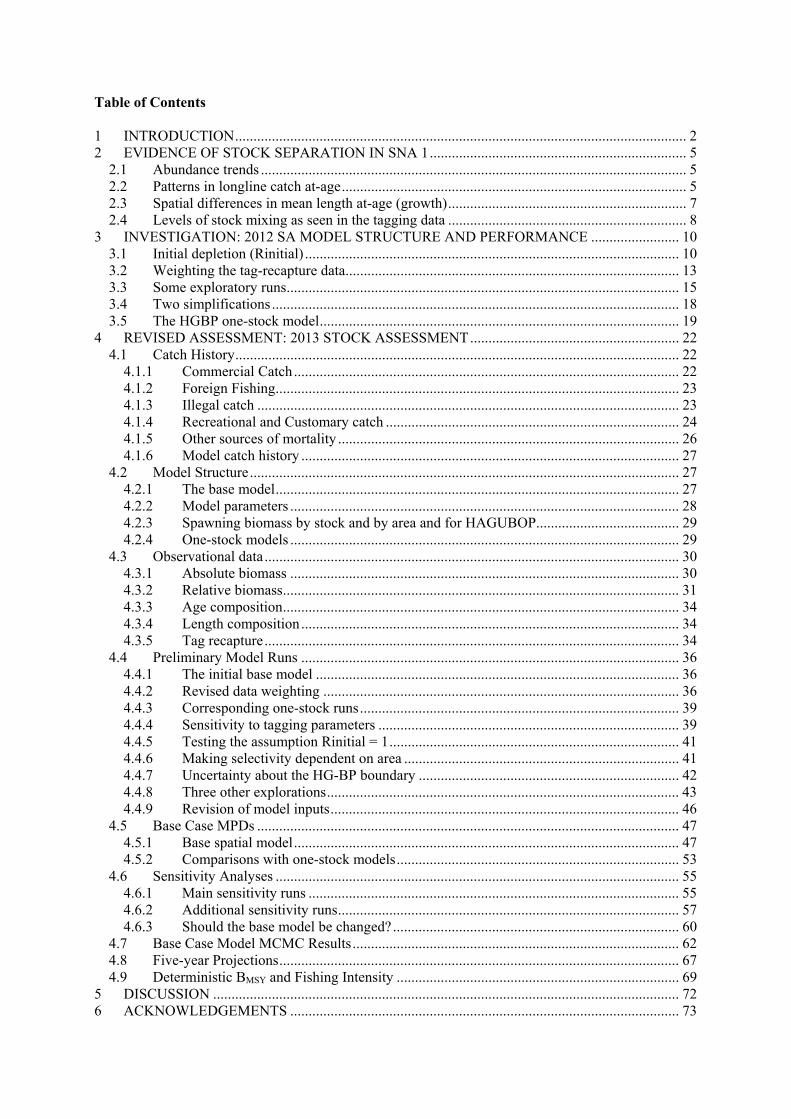
Table of Contents

1 INTRODUCTION........................................................................................................................... 22 EVIDENCE OF STOCK SEPARATION IN SNA 1...................................................................... 5

2.1 Abundance trends .................................................................................................................... 52.2 Patterns in longline catch at-age.............................................................................................. 52.3 Spatial differences in mean length at-age (growth) ................................................................. 72.4 Levels of stock mixing as seen in the tagging data ................................................................. 8

3 INVESTIGATION: 2012 SA MODEL STRUCTURE AND PERFORMANCE ........................ 103.1 Initial depletion (Rinitial) ...................................................................................................... 103.2 Weighting the tag-recapture data ........................................................................................... 133.3 Some exploratory runs........................................................................................................... 153.4 Two simplifications ............................................................................................................... 183.5 The HGBP one-stock model .................................................................................................. 19

4 REVISED ASSESSMENT: 2013 STOCK ASSESSMENT ......................................................... 224.1 Catch History......................................................................................................................... 22

4.1.1 Commercial Catch ......................................................................................................... 224.1.2 Foreign Fishing .............................................................................................................. 234.1.3 Illegal catch ................................................................................................................... 234.1.4 Recreational and Customary catch ................................................................................ 244.1.5 Other sources of mortality ............................................................................................. 264.1.6 Model catch history ....................................................................................................... 27

4.2 Model Structure ..................................................................................................................... 274.2.1 The base model .............................................................................................................. 274.2.2 Model parameters .......................................................................................................... 284.2.3 Spawning biomass by stock and by area and for HAGUBOP....................................... 294.2.4 One-stock models .......................................................................................................... 29

4.3 Observational data ................................................................................................................. 304.3.1 Absolute biomass .......................................................................................................... 304.3.2 Relative biomass............................................................................................................ 314.3.3 Age composition ............................................................................................................ 344.3.4 Length composition ....................................................................................................... 344.3.5 Tag recapture................................................................................................................. 34

4.4 Preliminary Model Runs ....................................................................................................... 364.4.1 The initial base model ................................................................................................... 364.4.2 Revised data weighting ................................................................................................. 364.4.3 Corresponding one-stock runs ....................................................................................... 394.4.4 Sensitivity to tagging parameters .................................................................................. 394.4.5 Testing the assumption Rinitial = 1 ............................................................................... 414.4.6 Making selectivity dependent on area ........................................................................... 414.4.7 Uncertainty about the HG-BP boundary ....................................................................... 424.4.8 Three other explorations................................................................................................ 434.4.9 Revision of model inputs ............................................................................................... 46

4.5 Base Case MPDs ................................................................................................................... 474.5.1 Base spatial model......................................................................................................... 474.5.2 Comparisons with one-stock models ............................................................................. 53

4.6 Sensitivity Analyses .............................................................................................................. 554.6.1 Main sensitivity runs ..................................................................................................... 554.6.2 Additional sensitivity runs ............................................................................................. 574.6.3 Should the base model be changed? .............................................................................. 60

4.7 Base Case Model MCMC Results......................................................................................... 624.8 Five-year Projections ............................................................................................................. 674.9 Deterministic BMSY and Fishing Intensity ............................................................................. 69

5 DISCUSSION ............................................................................................................................... 72ACKNOWLEDGEMENTS .......................................................................................................... 736

7 REFERENCES .............................................................................................................................. 738 APPENDICES ............................................................................................................................... 75

EXECUTIVE SUMMARY

Francis R.I.C.C.; McKenzie, J.R. (2015). Assessment of the SNA 1 stocks in 2013.

New Zealand Fisheries Assessment Report 2015/76. 82 p.

Snapper (Pagrus auratus) is New Zealand’s most valuable commercial coastal marine species and, by virtue of its high abundance around the populous regions of northern New Zealand, it is also the nation’s most important recreational species.

This report documents the stock assessment modelling carried out for SNA 1 during 2013, which builds on the incomplete 2012 assessment.

The base model started in 1900 and described 15 fisheries acting on three fish stocks, with annual migrations between three areas (east Northland, Hauraki Gulf, and Bay of Plenty). This model was fitted to five types of observation: absolute biomass (from the 1984 Bay of Plenty tagging experiment); relative biomass (from longline and trawl catch per unit effort, CPUE); age compositions from commercial fisheries and research surveys; length compositions from recreational fisheries; and recaptures from tagging experiments in 1984 and 1993. The 168 parameters estimated for this model described the unfished size and year-class strengths of each stock; the rates of migration; fishery and research selectivities; and catchabilities for the CPUE observations. Preliminary analyses are described which were useful in determining key aspects of the base model (including data weighting, the initial age structure, and trap shyness corrections for the tag recapture observations).

This assessment overcame the two major weaknesses identified in the 2012 assessment – poor estimation of initial depletion (Rinitial) and poor MCMC diagnostics – and developed an assessment which, despite some major uncertainties, can provide useful stock status information for fishery managers.

The 2013 base case assessments predicted both the east Northland and Hauraki Gulf stocks to be at 24% B0 in the 2012–13 fishing year; thus above the soft limit of 20% B0 but below the target of 40% B0. The Bay of Plenty stock was predicted to be at 6% B0 in 2013 i.e., below the hard limit of 10% B0. The combined status of the Hauraki Gulf and Bay of Plenty stocks in 2013 was 18% B0.

The major uncertainties that still exist relate to the location of stock boundaries, mixing and interchange rates, and area specific gear selectivities, the correct weighting of different data sets, and the significance of lower observed mean lengths in area BP. For these reasons the Working Group had greater confidence on the combined Hauraki Gulf/Bay of Plenty assessment result than the model results for the two areas separately. Various other uncertainties (e.g., effect of changing trap-shyness or tag-loss rates, or the maximum age in the partition) have were significantly reduced using suitable analyses in the 2013 assessment.

The predicted status of each of the three stocks in 2018 (five year projection outcomes) was for increasing or near-stable biomass, conditional on patterns of future recruitment being similar to those between 1996 and 2005 (i.e. above average). In contrast all stocks were predicted to decline between 2013 and 2018 when projections were undertaken resampling from the period representing mean recruitment. The decision as to which of these two projections should be given the greater credence depends on a subjective choice between two possible future recruitment patterns: above average or average. The Working Group felt recruitment variability over the projection period to 2018 was more likely to be similar to that of the preceding 10 years (above average) and placed greater emphasis on that projection outcome.

Ministry for Primary Industries Assessment of the SNA 1 stocks in 2013 1

1 INTRODUCTION

Snapper (Pagrus auratus) is New Zealand’s most valuable commercial coastal marine species and, by virtue of its high abundance around the populous regions of northern New Zealand, it is also the nation’s most important recreational species (Hartill et al. 2007). Most New Zealand snapper stocks have been subject to significant exploitation for over a century; national commercial landings peaked in the 1970s at around 18 000 t per annum (Paul & Sullivan 1988; Ministry of Fisheries 2008). Commercial exploitation of snapper has been constrained by quota since the introduction of the Quota Management System (QMS) in 1986. Non-commercial snapper exploitation is regulated primarily by minimum-legal-size and individual bag limits.

Under the QMS there are four snapper Quota Management Areas (QMAs) of commercial and non-commercial significance (Figure 1). The largest volume of catch, both commercial and non-commercial, comes from the east coast North Island QMA known as SNA 1 (Figure 1).

Figure 1: Boundaries for the snapper Quota Management Areas and three subareas within SNA 1: east Northland (EN), Hauraki Gulf (HG), and Bay of Plenty (BP).

Tagging movement, recruitment and growth data suggest that SNA 1 is productively distinct from the other three QMAs (Sullivan 1985; Walsh et al. 2011). Fishing pressure across SNA 1 has not been uniform and this is reflected in differences in age composition between SNA 1’s three component sub-areas: east Northland (EN); Hauraki Gulf (HG); Bay of Plenty (BP) (Paul 1977; Sullivan 1985; Davies & Walsh 1995: Figure 1). Recent east Northland longline catches show a wider range of age classes and a higher accumulation of biomass older than 20 years than catches from the other areas, suggesting that it has been less intensely fished (Walsh et al. 2011). The smallest proportion of biomass in the older age

2 Assessment of the SNA 1 stocks in 2013 Ministry for Primary Industries

classes is seen in Bay of Plenty catches (Walsh et al. 2011), which is believed to be a legacy of a relatively high level of trawl fishing during the 1970s. Despite spatial differences in productivity, tagging observations suggest that the level of mixing between the three sub-stocks is significant; especially between Hauraki Gulf and the Bay of Plenty (Sullivan et al. 1988; Gilbert & McKenzie 1999). The areas also appear to have similar recruitment characteristics (Walsh et al. 2011).

The spatial complexity of SNA 1 makes it difficult to assess as a unit stock. One approach has been to assess SNA 1 using amalgamated data from either two sub-stocks or all three. Another approach has been to model each sub-stock independently; the overall SNA 1 yield statistic being the combination of the individual assessments. Both approaches have problems; amalgamation results in an assessment inherently more uncertain because spatial variability is unaccounted for. Assessing the sub-stocks independently, although accounting for spatial variability, ignores between-area movements and may lead to a biased assessment.

Many millions of dollars have been spent monitoring SNA 1 since the early 1980s. Monitoring programmes have included commercial catch-at-age sampling, recreational harvest surveys, trawl surveys, and tagging programmes to derive estimates of biomass. Age-structured population modelling is used to estimate its productivity and status of the SNA1 Fishstock.

An assessment of SNA 1 was undertaken in April 2012 using a spatially disaggregated movement model (Francis & McKenzie 2015). The main structural differences between the previous 1999 (Gilbert et al. 2000) and the 2012 SNA 1 assessment were: - Separation of Bay of Plenty and Hauraki Gulf sub-stocks; - Incorporation of a Beverton & Holt stock recruitment relationship (h = 0.85; note: no stock

recruit relationship was assumed in the 1999 SNA 1 assessment).

The deterministic BMSY from the 2012 assessment was 26–27% B0 for all stocks and areas compared to 20% B0 in the 1999 assessment; the inclusion of a stock recruit dynamic is largely responsible for the difference in the deterministic BMSY/B0 ratios between the two assessments (Hilborn & Stokes 2010; McKenzie 2012).

In the 2012 assessment all three SNA 1 stocks were estimated to be below BMSY with east Northland at 15–17% B0; Hauraki Gulf at 12–14% B0 and the Bay of Plenty at 5–6 % B0, with no sub-area likely to rebuild in the next five years.

The 2012 assessment model commenced in 1970 with all three stocks in an exploited state; to do this required estimating an offset parameter [Rinitial] on mean recruitment (Francis & McKenzie 2015; Bull et al. 2012).

Two model performance issues were identified in the 2012 assessment: 1. Poor estimation of initial depletion (Rinitial); 2. Poor MCMC convergence.

There was insufficient time during the 2012 assessment period to fully investigate these and other aspects of model performance. Although the 2012 SNA 1 model made significant progress toward achieving a robust SNA 1 assessment, the Northern Inshore Working Group (hence forth denoted as Working Group) felt that further investigations were needed to resolve the performance issues before the results could be considered useful for management.

The Working Group concluded that there were two aspects of the 2012 assessment that needed further investigation:

1. The validity of the “three stock” hypothesis in particular the degree of stock separation between snapper in the Hauraki Gulf and Bay of Plenty areas;

2. Resolution of 2012 model performance issues.


In light of NINSWG recommendations, four additional objectives were added to the SNA201101 project the results of which are presented in this report:

1. To investigate historical catch-at-age and tagging data for evidence of spatial pattern consistent or otherwise with the 2012 SNA 1 assessment model spatial structure (Section 2).

2. To update the current SNA 1 longline and trawl CPUE to include the 2011–12 fishing year (Section 4.3.2).

3. To investigate ways to improve the performance of the current (2012) spatially disaggregated SNA 1 assessment model, specifically: model robustness to initial starting assumptions and the generation of suitable Bayesian posteriors (Section 3).

4. To conduct a stock assessment for SNA 1 in the 2012 fishing-year using spatially disaggregated age-structured modelling, including estimating biomass and sustainable yields (Section 4).

Each objective has its own section in this report. The 2012 assessment is described in Francis and McKenzie (2015).


2 EVIDENCE OF STOCK SEPARATION IN SNA 1

2.1 Abundance trends

East Northland longline CPUE abundance indices (McKenzie & Parsons 2012) correlate poorly with indices from both Hauraki Gulf and Bay of Plenty (Table 1); poor correlation in relative abundance with other SNA 1 areas is evidence in support of east Northland being a separate stock. In contrast, Hauraki Gulf and Bay of Plenty CPUE abundance trends were reasonable well correlated (Table 1), a result inconsistent with a separate stock hypothesis.

Table 1: Pearson correlations of SNA 1 bottom longline CPUE indices given in McKenzie & Parsons 2012.

Hauraki Gulf Bay of Plenty

East Northland 0.119 [P < 0.598] 0.267 [P < 0.23]

Hauraki Gulf - 0.882 [P < 0.000]

2.2 Patterns in longline catch at-age

Patterns seen in the approximately 20 year time series of longline catch at-age observations from SNA 1 show consistently higher proportions of 20+ cumulative age classes in east Northland compared to the Hauraki Gulf and Bay of Plenty (Figure 2). The persistence of older age classes in east Northland suggests that historical fishing pressures were significantly lower in this area than in the other two areas. The preservation of the low total mortality signal in the east Northland series is indicative of a low level of mixing between this and the other two areas i.e. of east Northland being a separate stock.

Multiple consecutive years of catch sampling provide multiple observations of the individual year classes and therefore these data provide a high degree of power to estimate relative year class strength (YCS) across SNA 1. Although some spatial differences in YCS were evident in the data (Figure 3), YCS patterns across all three SNA 1 areas were reasonably well correlated (Table 2). Although this result is inconsistent with the multiple SNA 1 stock hypothesis, it does not refute this hypothesis either, as it is possible the three SNA 1 stocks may be exhibiting similar recruitment responses to common broad climatic trends (e.g. changes in the Southern Oscillation Index).


1990 1989 1988 1987 1986 1985

East Northland Bay of Plenty

1965 1966 1965

1967 1966

1968 1967

1969 1968

1970 1969

1971 1970

1972 1971

1973 1972

1974 1973

1975 1974 1975 1976 1976 1977 1977

1978 1978

1979 1979

1980 1980

1981 1981

1982 1982

1983 1983 1984 1984

yea

r cl

ass

yea

r cl

ass

1985 1986 1987 1988 1989 1990

1991 1992

1991

1993 1992

1994 1993

1995 1994

1996 1995

1997 1996

1998 1997 1998

1999 1999 2000 2000 2001 2001 2002 2002 2003 2003

2004 2004

2005 2005

2006 2006

2007 2007

2008 2008

2009 2009

1985 1986 1987 1988 1989 1990 1991 1992 1993 1994 1995 1996 1997 1998 1999 2000 2001 2002 2003 2004 2005 2006 2007 2008 2009 2010

fishing year

1985 1986 1987 1988 1989 1990 1991 1992 1993 1994 1995 1996 1997 1998 1999 2000 2001 2002 2003 2004 2005 2006 2007 2008 2009 2010

fishing year

Hauraki Gulf 1965 1966

1968 1967

1969

1971

1973

1970

1972

1974

1976

1978

1975

1977

1979

1981

1983

1980

1982

1984

yea

r cl

ass

1985 1986

1988 1987

1989

1991

1993

1990

1992

1994

1996

1998

1995

1997

1999

2001

2003

2000

2002

2004

2006

2008

2005

2007

2009

1985 1986 1987 1988 1989 1990 1991 1992 1993 1994 1995 1996 1997 1998 1999 2000 2001 2002 2003 2004 2005 2006 2007 2008 2009 2010

fishing year Figure 2: Time series of age frequency distributions by year class and year from the SNA 1 bottom

longline spring¬-summer fishery from 1984–85 to 2009–10. Symbol area is proportional to the proportion at age. The proportion of the oldest year class in each year is represented by an aggregate (over 19 years) age group (reproduced from Walsh et al. 2011).

Table 2: Pearson correlation of SNA 1 area bottom longline year class deviates from longline catch-at-age

sampling (Figure 3; Walsh et al. 2011).

Hauraki Gulf Bay of Plenty

East Northland 0.568 [P < 0.003] 0.734 [P < 0.000]

Hauraki Gulf - 0.798 [P < 0.000]


East Northland

Ye

ar

Cla

ss S

tre

ng

th

YC

S

YC

S

YC

S

0.0

0.5

1.0

1.5

2.0

2.5

3.0

3.5

4.0

4.5

5.0

5.5

6.0

6.5

0.0

0.5

1.0

1.5

2.0

2.5

3.

0

3.5

4.0

4.

5

5.0

5.5

6.0

0.5

1.0

1.5

2.0

2.5

3.0

1977 1979 1981 1983 1985 1987 1989 1991 1993 1995 1997 1999 2001

Yclass

Hauraki Gulf

1977 1979 1981 1983 1985 1987 1989 1991 1993 1995 1997 1999 2001

Yclass

Bay of Plenty

1977 1979 1981 1983 1985 1987 1989 1991 1993 1995 1997 1999 2001

Year Class Yclass

Figure 3: Relative difference in Year Class Strength (YCS) derived from multiple years of longline catch-

at-age sampling. Year class indices are expressed as log deviates from the predicted log-linear catch-at-age decay rate (catch curve) in each sampling year. Dotted lines are the individual year deviates; large dots denote where the 95% CI on the median YCS does not include 1 (i.e. we are 95% confident of the YC being either strong or weak). Vertical dotted lines are examples of significant differences in YCS between areas.

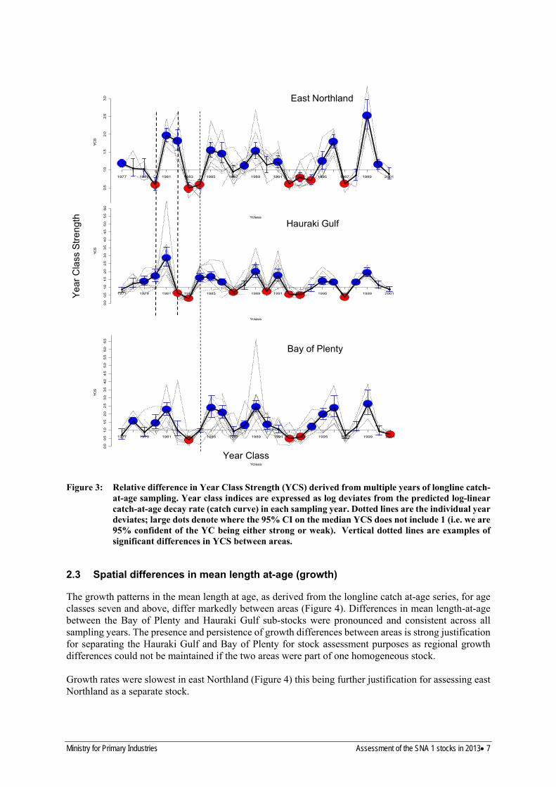
2.3 Spatial differences in mean length at-age (growth)

The growth patterns in the mean length at age, as derived from the longline catch at-age series, for age classes seven and above, differ markedly between areas (Figure 4). Differences in mean length-at-age between the Bay of Plenty and Hauraki Gulf sub-stocks were pronounced and consistent across all sampling years. The presence and persistence of growth differences between areas is strong justification for separating the Hauraki Gulf and Bay of Plenty for stock assessment purposes as regional growth differences could not be maintained if the two areas were part of one homogeneous stock. Growth rates were slowest in east Northland (Figure 4) this being further justification for assessing east Northland as a separate stock.


Also seen in the data is a systematic decline in mean-length-at-age across all age classes in all three areas.

ENLD HAGU BPLE

0

Me

an

len

gth

at a

ge

(cm

)

30

4

05

06

0

30

4

05

06

0

30

4

05

06

0

0 00 0 0

000 00 00

900 0 990 0 90 800 8 80 0800 9 90 0 7 7 97 08 0 00 7 80 99 90 6 90 80 7 87 80 6 6 990 0 0 9 8 9 8 5 6 700 7 88 600 9 80 8 6 60 5 777 64 500 9 7 9 90 5 959 958 9 6 69 57 7 58 8 88 86 48 388 6 5 457 4 7 09 79 7 99 9 9 46 4 47 6 7 7 79 48 9 68 8 7 8 869 5 4 4 38 698 6 99

8 59 2 367 9 7 6 87 98 6 76 59 9 3 707 5 5 88

7 385 7 39 586 6 6 37 7 8 3 38 6 37 5 28 765 5 48

7 46 9

8 647 98 5 77 6 46 6 6 5 5 5 76 1 4 655 7 2 24984 4 9

8 5 26 6 5 4 2 27 1 3 535 5 5 4 67 24 4 5 6 598 6 5 6 247 6 4 235 9

8 4 9

8 3 45 7984 64 4 34 37

66 5 3 5 1 42 45 3 533 6 5 44 0 13 4 1 1 245 7 5

6 74 3 3 17 33 33 4 03 5 1 253 4 33 4 42 6 34 2 4 982 12 4 63 12 3 14 3 43 5 23 2 132 2 76 02 5 0 033 2 52 22 2 33 4 13 3 3 3 092 0 21 2 51 4 91 2 22 02 4 01 2 131 2 2 1 41 02 221 1 02 1 1 23 01 2 91 3 93 9 01 12 1 11 00 0 1 1 10 1 1 12 1 20 9 91 0 90 8 9 80 2 90 0 11 1 100 100 0 1 00 90 1 0 990 099 0 0 80 8 89 9 0 0 19 0 0 9 9 999 9 0 00 89 99 99 0 8 80 80 8 979 99 99 0 79 9 9 88 9 9 988 8 9 89 88 98 79 9 7 798 8 98 88 8 98 79 9 88 78 8 78 8 8 7 78 88 8 77 87 77 8 87 8 8 87 7 78 77 7 7 8 87 7 88 77 77 77 77

7 7 77 7 77 777 7 7 7 77

1995 2000 2005 2010 1995 2000 2005 2010 1995 2000 2005 2010 Figure 4: Mean lengths at age (for ages 1 to 20+) by area. The plotting symbols identify the age class (e.g.,

‘1’ is used both 1- and 11-year olds). Trends in these mean lengths are shown by regression lines (red dotted lines).

2.4 Levels of stock mixing as seen in the tagging data

There have been a number of large tag release events across SNA 1; these date back to the mid 1970s (Crossland 1976). The tagging results suggest that although there is movement of fish between the SNA 1 sub-areas, large (more than 100 nautical mile) distance movements are relatively rare in the data series (Sullivan et al. 1988.; McKenzie & Davies 1996). During the 1984–85 fishing year a tagging programme for biomass estimation took place across the Hauraki Gulf and east Northland areas (Sullivan et al. 1988). A second biomass tagging programme was undertaken during the 1993–94 fishing year across all three SNA 1 areas (McKenzie & Davies 1996). Although tagging data is available from other release events in SNA 1 it was only in the 1985 and 1994 programmes where tagging occurred concurrently in more than one area, thus allowing inter-area movement rates to be estimated: the 1985 tagging data allows mixing rates between Hauraki Gulf and East Northland to be estimated; the 1994 tagging data allows movement between all three areas to be estimated (Table 3). Table 3: Numbers of fish tagged and recaptured by area in the 1985 and 1994 tagging experiments Recaptured 1985 Tagged EN HG BP EN 6 782 418 29 - HG 12 046 47 974 -1994 EN 8 190 129 10 5 HG 13 466 20 272 17 BP 3 630 2 25 41


7 7 7

8 8 8

0 0 0

1 1 1

2

2 2

3

4

5

6

7

0

The 1994 tagging results suggest relatively low interchange between the Hauraki Gulf and Bay of Plenty (Table 3); the 2012 assessment’s poor prognosis for the Bay of Plenty stock is in part driven by the low rate of tag-inferred mixing from these data (Francis & McKenzie 2015).

In conclusion; evidence that East Northland snapper is a distinct biological stock is based on differences seen in age structure, biomass trend, growth rates and tag mixing rates. Evidence that the Bay of Plenty snapper are relatively distinct from Hauraki Gulf snapper biologically is based on higher snapper growth rates in the Bay of Plenty and relatively low levels of tag mixing. It was deemed preferable to model SNA 1 as three spatially disaggregated biological stocks with allowance for spatial mixing between the three stock areas to accommodate the level of interchange observed in the tag recovery data.

An aspect of uncertainty in the 1994 tagging data was the location of the “true” boundary between the Hauraki Gulf and Bay of Plenty stocks. The highest spatial resolution in the 1994 tagging data was to statistical reporting area level (Figure 5). In the 2012 assessment Statistical Area 008 was deemed to be part of the Bay of Plenty sub-stock. Anecdotal evidence from NIWA longline catch sampling programmes (C. Walsh pers. comm.) suggests that the region of Statistical Area 008 behind Great Barrier and north of Cape Colville is more similar to the Hauraki Gulf age-structure, whereas the region of area 008 to the south is more consistent with Bay of Plenty age structures (008 North and 008 South Figure 5). It is not possible to assign Statistical Area 008 tag recoveries at a finer spatial scale, meaning that tag release and recovery observations from this stat area are potentially ambiguous. A sensitivity analysis to this stock boundary assumption was undertaken in the 2013 updated assessment whereby all tag and release observations from and to Statistical Area 008 were removed from the data (see Section 4.4.7).

34°

30'

35°

30'

36°

30'

37°

30'

38°S

174°E 176° 178°

004

002

005

003

006

007

009 010

SNA 1

SNA 8

008 North

008 South

Figure 5: SNA 1 statistical reporting areas representing the highest spatial resolution in the catch-at-age and tagging data.


3 INVESTIGATION: 2012 SA MODEL STRUCTURE AND PERFORMANCE

The base model is a development of the spatially disaggregated model proposed by McKenzie (2012). The McKenzie model recognises SNA 1 as being comprised of three separate biological stocks and uses a home fidelity (HF) dynamic to model movement of these stocks between three spatial areas: East Northland, Hauraki Gulf; Bay of Plenty (Figure 1). Under the HF dynamic, movement is an attribute of the individual fish not the area in which it currently resides; stocks and areas can therefore be decoupled such that during some of the model time steps a given area may contain fish from one or more stocks. The HF decoupling property meant that the model could provide yield estimates (MSY, BMSY, B0, etc) relative to both stocks and areas. To avoid confusion about areas and stocks we will use two-letter abbreviations (EN, HG, BP) for areas, and longer abbreviations (ENLD, HAGU, BOP) to denote biological stocks.

In this section we describe investigations into model performance that were carried out after the 2012 assessment. We provide labels for each of these additional runs, but, in the interests of brevity, we make no attempt to document all the ways in which they differed from the 2012 base run (refer Francis & McKenzie (2015) for model description, naming conventions, and data summaries). Method codes referenced in tables and figures are: longline (LL), bottom or single trawl (BT or ST), Danish seine (DS), recreational line (REC), research trawl (RES), all other methods (OTH).

3.1 Initial depletion (Rinitial)

Two runs were done in an attempt to address the weakness of poor estimates of Rinitial estimates in the 2012 base run model (Francis & McKenzie 2015).

In the first, base85, the initial year of the model was moved to 1985. This is the latest initial year that allows use of the tag-recapture observations, and it brings more age- and length-composition data sets closer to the initial year (Figure 6) which it was hoped would strengthen estimates of Rinitial.

Abundance Age HG_Res_abund83_01 x xxxxxxx xxx x x HG_ST_age xx x xx x

HG_LL_age x xxxxxxxxxxxxxxxxxxxxx HG_LLcpue90_11 xxxxxxxxxxxxxxxxxxxxxx HG_DS_age xxxx xx x x xxx

EN_LL_age x xxxxxxxxxxxxxxxxx xxxxxxxxxxxxxxxxxxxxxx EN_LLcpue90_11 xx xxxxxxxxxxxxxxxxx BP_LL_age

BP_LLcpue90_11 xxxxxxxxxxxxxxxxxxxx x BP_BT_ageBP_DS_age

xxx x x

BP_BTcpue96_11 xxxxxxxxxxxxxxxx EN_RES_ageHG_RES_age

x xxx xxx xxx x

BP_Tag_bio x BP_RES_age xx x

1970 1980 1990 2000 2010 1970 1980 1990 2000 2010

Length HG_REC_len_pre95 x x

HG_REC_len_post95 x xxxxxxxxx x

EN_REC_len_pre95 x x

EN_REC_len_post95 x xxxxxxxxx x

BP_REC_len_pre95 x x

BP_REC_len_post95 x xxxxxxxxx x

1970 1980 1990 2000 2010

Figure 6: Illustration of the years associated with all non-tagging observations in the base model. Those observations to the left of the dotted line were omitted in run base85, which included all tag-recapture observations (because these were in 1985, 1986, 1994, and 1995).

Run base85 produced similar estimates of stock status (current biomass as %B0 for stocks ENLD, HAGU, and BOP changed from 17, 15, and 4, respectively, in the base run to 19, 19, and 3). However,


this is not an improvement on the base run because profiles on the Rinitial parameters showed that these parameters were not, as hoped, primarily determined by the composition data (Table 4).

Table 4: The individual objective-function components that are most influential in determining lower and upper bounds for the parameter Rinitial in each of the three stocks for run base85.

ENLD HAGU BOP Lower prior on ENLD YCS prior on HAGU YCS prior on BOP YCS Upper EN_LLcpue90_11 HG_LLcpue90_11 1994HAGU_HAGU_Tags

In the second run addressing the problem of initial depletion the initial year was moved back to 1900 and it was assumed that there was no initial depletion at that time (i.e., Rinitial = 1, so the initial SSB was equal to B0). To deal with uncertainty in the early catches three alternative pre-1970 catch histories were used for each stock – low, medium, and high – and the associated model runs were labelled base00lo, base00, and base00hi.

The commercial components of the pre-1970 catch histories for these runs were derived from the catches used by Davies (1999) in the 1997–98 assessment. That assessment was for two areas: EN and HG-BP combined, so for present purposes the catches for the latter area were split in the ratio 78:22 (HG:BP), which is the average ratio of reported commercial catches from the two areas since 1970. In constructing catch histories for the Japanese longline fleet Davies (1999) considered three alternative levels for the cumulative totals from this fishery: 20 000 t, 30 000 t, and 50 000 t. We used only the middle of these three but, to allow for uncertainty in this catch, as well as under-reporting in the New Zealand catches, the Davies (1999) catch history was used in base00lo, and this was multiplied by factors of 1.2 and 1.5 to make the commercial catch histories for base00 and base00hi, respectively.

Recreational catches were assumed to decline linearly from the 1970 levels used in the base run to assumed levels in 1900. Low, medium, and high values for the 1900 catches were derived from expert opinion (pers. comm., John Holdsworth and Bruce Hartill) (Table 5).

All three combined catch histories (commercial + recreational) peaked around 1970 and were at much lower levels in 1900 (Figure 7). The catches assumed for 1900 do not appear inconsistent with pre-European snapper catches estimated by Smith (2011) (Table 6).

Table 5: Assumed quantities used in deriving pre-1970 catch histories for runs base00lo, base00, and base00hi.

Catch Multiplier for Assumed 1900 recreational catch (t) history commercial catches1 EN HG BP Low 1.0 50 100 50 Medium 1.2 75 150 75 High 1.5 100 200 100 1A commercial catch history derived from Davies (1999) (see text for details) was multiplied by these multipliers to generate low, medium, and high catch histories.


EN

0

1

2

3

4 base00hi base00 base00lo

Cat

ches

('0

00 t

)

1900 1920 1940 1960 1980 2000

0 2 4 6 8

10 12 14

HG

1900 1920 1940 1960 1980 2000

BP

0

1

2

3

4

1900 1920 1940 1960 1980 2000

Figure 7: Catch histories for runs base00lo, base00, and base00hi.

Table 6: Comparison between pre-European snapper catches (t) calculated by Smith (2011) for the ‘Greater Hauraki Gulf’ (roughly from Whangarei to Tauranga – see figure 1 of Smith 2011) and those used for 1900 in runs base00lo, base00, and base00hi.

Year 1400

Area Greater HG

Low Estimated ca

Medium 72

tches (t) High

1550 Greater HG 940 1750 Greater HG 997 1900 HG 1152 1412 1780

HG + BP 1499 1844 2326 HG + BP + EN 1700 2100 2653

The alternative catch histories had relatively little effect on estimated biomass trajectories (Figure 8, left panels), which were quite similar to those from the base run for ENLD and HAGU, and markedly higher for BOP (Figure 8, right panels).


200 200

150 150

100 100

50 50

0 0

ENLD HAGU BOP

base00hi base00 base00lo

1900 1920 1940 1960 1980 2000

ENLD HAGU BOP

base base00

1900 1920 1940 1960 1980 2000

B0

(%

B0)

B

0 ('0

00 t

)

100

80

60

40

20

0 1900 1920 1940 1960 1980 2000

100

80

60

40

20

0 1900 1920 1940 1960 1980 2000

Figure 8: Comparison of estimated SSB trajectories from run base00 with those from base00lo and base00hi (left panels) and those from base (right panels).

A strength of base00 is that there is no longer a need to estimate Rinitial for each stock because it is assumed to be 1. To evaluate the appropriateness of this assumption we simulated fishing in a model whose structure and parameters were the same as assumed and estimated for base00 except that (a) catches were constant, at the levels assumed in base00 for 1900; and (b) recruitment was deterministic (i.e. all YCSs were set to 1). In this simulation the equilibrium SSBs were found to be 96, 89, and 90%B0 for ENLD, HAGU, and BOP, respectively. We then reran base00 after setting Rinitial for the three stocks to 0.96, 0.89, and 0.90, respectively. The effect of this modification on current stock status was minimal: changes in estimated Bcurrent as %B0 were only about 0.1% for all stocks.

The WG concluded that the best way to solve the problem of Rinitial is to move the initial year back to 1900 and set Rinitial to 1.

3.2 Weighting the tag-recapture data

Two modifications were considered to the weighting of the tag-recapture data.

The first modification concerned the number of length classes used for each of the 26 tag-recapture data sets (Francis & McKenzie 2015). In modelling programme CASAL (Bull et al. 2012), there is complete freedom to specify the length classes for each tag-recapture data set, and once these are specified the user provides, for each length class, the number of fish scanned for tags and the number of tags found. In the base model, 1 cm length classes were used, with an average of 51 length classes per data set. This seemed far too many length classes, considering that the total number of tags found (across all length classes) was less than 10 in 12 of the 26 data sets. It seemed sensible to condense these data sets by increasing the widths of the length classes in such a way that there would be fewer classes in data sets with fewer recaptures. In run base.cond this was done by combining adjacent length classes until each


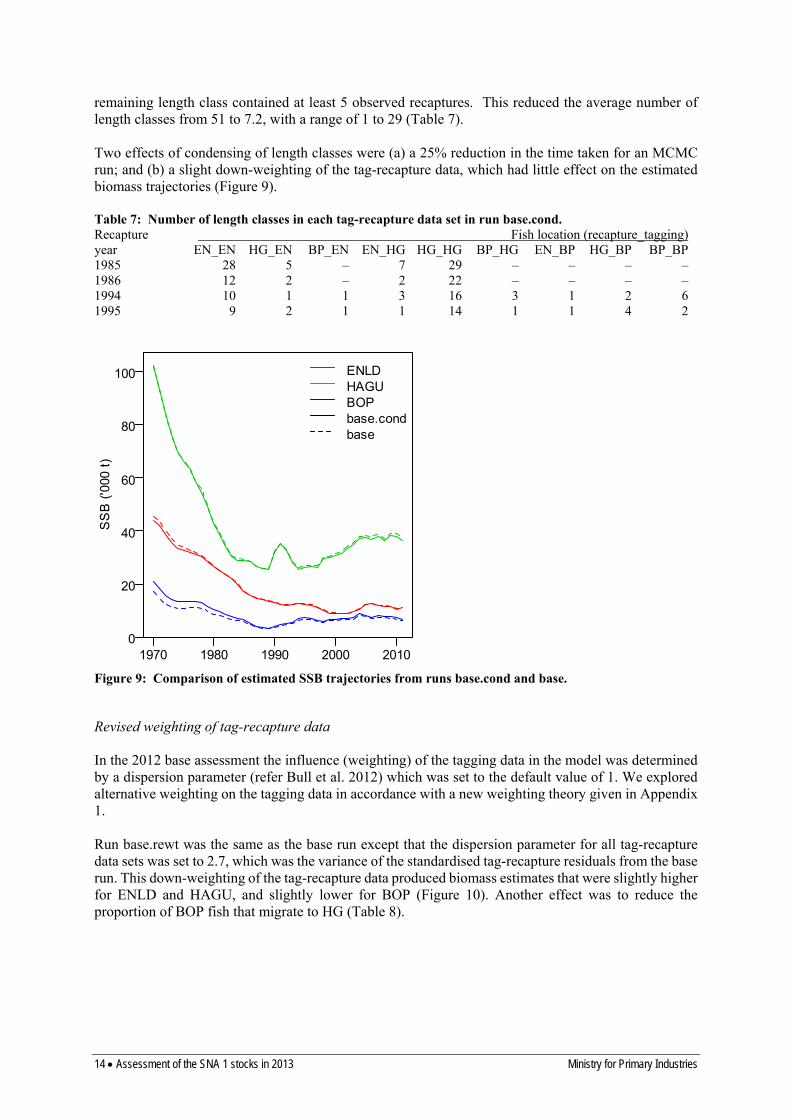
remaining length class contained at least 5 observed recaptures. This reduced the average number of length classes from 51 to 7.2, with a range of 1 to 29 (Table 7).

Two effects of condensing of length classes were (a) a 25% reduction in the time taken for an MCMC run; and (b) a slight down-weighting of the tag-recapture data, which had little effect on the estimated biomass trajectories (Figure 9).

Table 7: Number of length classes in each tag-recapture data set in run base.cond. Recapture Fish location (recapture_tagging) year EN_EN HG_EN BP_EN EN_HG HG_HG BP_HG EN_BP HG_BP BP_BP 1985 28 5 – 7 29 – – – – 1986 12 2 – 2 22 – – – – 1994 10 1 1 3 16 3 1 2 6 1995 9 2 1 1 14 1 1 4 2

SS

B (

'000

t)

100

80

60

40

20

0

ENLD HAGU BOP base.cond base

1970 1980 1990 2000 2010

Figure 9: Comparison of estimated SSB trajectories from runs base.cond and base.

Revised weighting of tag-recapture data

In the 2012 base assessment the influence (weighting) of the tagging data in the model was determined by a dispersion parameter (refer Bull et al. 2012) which was set to the default value of 1. We explored alternative weighting on the tagging data in accordance with a new weighting theory given in Appendix 1.

Run base.rewt was the same as the base run except that the dispersion parameter for all tag-recapture data sets was set to 2.7, which was the variance of the standardised tag-recapture residuals from the base run. This down-weighting of the tag-recapture data produced biomass estimates that were slightly higher for ENLD and HAGU, and slightly lower for BOP (Figure 10). Another effect was to reduce the proportion of BOP fish that migrate to HG (Table 8).


Table 8: Comparison of estimated migration matrices from runs base.rewt and base, with underlined numbers showing the greatest between-run differences. The tabulated numbers are the proportions of each stock migrating to each area in time step 2.

base.rewt base Area

Stock EN HG BP EN HG BP ENLD 0.94 0.05 0.01 0.94 0.04 0.02 HAGU 0.06 0.90 0.04 0.07 0.89 0.04 BOP 0.04 0.23 0.73 0.03 0.27 0.70

ENLD HAGU BOP

50base rewt

100 1540

80

30 60 10

20 40 5

10 20

0 0 0 1970 1990 2010 1970 1990 2010 1970 1990 2010

1470 4060 12

30 1050

8 20

40

630

420 1010 2

0 0 0 1970 1990 2010 1970 1990 2010 1970 1990 2010

Figure 10: Comparison of estimated SSB trajectories from runs base and base.rewt.

3.3 Some exploratory runs

A useful way of understanding the effect of different data types in an assessment is to down-weight them one at a time and see how the assessment outputs change. This was done for the four data types in the base assessment (Table 9).

The effects on SSBs of these changes in weighting are shown in Figure 11. The first thing to note is that the effects were least for ENLD and HAGU and greatest for BOP. This tells us that biomass estimates are more robust for ENLD and HAGU, and less robust for BOP. The other striking result – most apparent for ENLD and HAGU in recent years – is the conflict between the age and tagging data: recent SSBs for these stocks increase when the tagging data are down-weighted, and decrease when age data are down-weighted. The effect on BOP SSB is more complex but reversed, in the sense that recent SSBs are lower when the tagging data are down-weighted, and higher when age data are down-weighted.

SS

Bs

(%B

0)

SS

Bs

('000

t)


Table 9: Description of four variants of the base run in which one type of data was down-weighted.

Run base.dwtage base.dwtlen base.dwtabund

base.dwttag

Change from base multinomial Ns for at-age observations divided by 10 multinomial Ns for at-length observations divided by 10 for abundance observations, cv set to 1 (for CPUE and BP_Tcv_process_error set to 1 (for HG_Res_abund83_01) dispersion parameter for tag-recapture data increased from 1

ag_bio) or

to 10

ENLD HAGU BOP

50

40

30

20

10

0

base dwtage dwtabund dwtlen dwttag

120

100

80

60

40

20

0

20

15

10

5

0

SS

Bs

(%B

0)

SS

Bs

('000

t)

1970 1990 2010 1970 1990 2010 1970 1990 2010

80

60

40

20

0

50

40

30

20

10

0

15

10

5

0 1970 1990 2010 1970 1990 2010 1970 1990 2010

Figure 11: Effect on estimated SSB trajectories of down-weighting all data sets of one type (the types are age, abundance, length, and tagging).

We can summarise the conflict between the age and tagging data sets by saying that the age data favours higher SSBs for ENLD and HAGU and lower SSB for BOP, and the tagging data favours the opposite. One reason for this complex relationship is that the SSB trajectories are affected not only by the initial SSBs (determined by R0 and Rinitial for each stock), but also by the migration matrix. Down-weighting either age or tagging data has strong effects on this matrix, and particularly on the parameters describing movement between HG and BP (Table 10).

Table 10: Comparison of estimated migration matrices from the base run and two others (base.dwtage and base.dwttag), with underlined numbers showing the greatest differences from the base run. The tabulated numbers are the proportions of each stock migrating to each area in time step 2.

base base.dwtage base.dwttag Area

Stock EN HG BP EN HG BP EN HG BP ENLD 0.94 0.04 0.02 0.93 0.04 0.02 0.94 0.05 0.01 HAGU 0.07 0.89 0.04 0.07 0.86 0.07 0.05 0.91 0.04 BOP 0.03 0.27 0.70 0.03 0.30 0.67 0.04 0.13 0.83


Imbalance in tag-recapture fits

Examination of these runs revealed a previously unnoticed imbalance in the tag-recapture fits. In the 2012 base run, the observed number of recaptures is greater than the expected number for 18 of the 26 tag-recapture data sets (this is shown in figure 23 of Francis & McKenzie (2015), where the observed value, ‘o’, is to the left of the expected value, ‘×’, in 18/26 data sets). The same imbalance occurred in the one-stock models where observed is greater than expected in 9 of 10 data sets (Francis & McKenzie 2015). Moreover, the imbalance persists, with one exception, if we consider subsets of the tag-recapture data sets defined by either tagging or recapture location: the exception is that observed is greater than expected in only 4 of the 6 data sets for fish tagged in BP. As might be expected, the imbalance is worse (23/26) in run base.dwttag, and better (13/13) in run base.dwtage.

Relative depletion signal in the composition data

Another previously unnoticed feature of the 2012 assessment was the relative depletion signal in the composition data. For each fishing method, the observed mean ages tend to be highest in area EN, a bit lower in HG, and lowest in BP (Figure 12). Because the selectivity for each fishing method is assumed to be the same in all areas this suggests that the population is least depleted in EN and most depleted in BP.

LL age RES age ST age x x x5.5x x11 EN 9x xxHG x5.0x xx xxBP x x xx10 x x x 8x xxx x xx x

xx 4.5 xx xxx x xxxxxx x x9 x xxx x4.0x x x x x

xxx x 7xx xx xx8 x xxx 3.5x x x xxx 6xxxx

x 3.0 x

x 7 x

1970 1990 2010 1970 1990 2010 1970 1990 2010

DS age REC length REC age xx xx10x x36

x x xx xx xx xxxxxxx x x xx 9 x xxx x x xx xx x34 xxx x xx xxxx xxxx 8

x xx x xx x xxx xx xxx x32 x x xx7 xxxx x x30 6x x 7

8

9

10

11

12

13

14 x

x x

x x

x

x

xxx x

x

Obs

erve

d m

ean

age

or le

ngth

1970 1990 2010 1970 1990 2010 1970 1990 2010

Figure 12: Observed mean age or length by fishing method and area. In the bottom right-hand panel, the observed recreational mean lengths have been converted to ages using the mean length at age relationship (averaged over years 1994–2010) for each area.

We evaluated the influence of this relative depletion signal with run base00sel, which was the same as base00 except that the assumption that selectivity for each method is independent of area was dropped (which meant estimating 16 selectivity curves, instead of the 6 estimated in base00; because of lack of catch at age data, selectivities for methods ST and DS in EN were assumed to be the same as for HG). This change had relatively little effect on estimated SSB trajectories, but produced estimates of current depletion that were similar to those from one-stock runs (Figure 13). Note that several of the selectivities


estimated in base00sel were not well determined because of limited data (e.g., there is only one year’scatch at age data for DS in area BP and RES in area EN).

SS

B (

%B

0)

SS

B (

'000

t)

ENLD or EN HAGU or HG BOP or BP

80200

base00 base00sel onestock

100

60 80150

6040 10040

20 50 20

0 0 01900 1940 1980 1900 1940 1980 1900 1940 1980

100 100 100

80 80 80

60 60 60

40 40 40

20 20 20

0 0 0 1900 1940 1980 1900 1940 1980 1900 1940 1980

Figure 13: Comparison of SSBs by stock from runs base00 and base00sel with SSBs from corresponding one-stock runs (which bear the same relationship to run base00 as the 2012 one-stock runs do to the base run).

3.4 Two simplifications

Two simplifications to the base model were considered and accepted by the Working Group. The first was to drop five fisheries which contributed only a small percentage of the catch to an area and for which there was no age or length composition data (Table 11). In run base.drop.fisheries these fisheries were dropped and their catches distributed pro rata across the other fishing methods in the area. The effect on estimated SSBs was minor (Figure 14) and there was a very slight overall improvement in goodness of fit (by 0.8 objective function points).

Table 11: Average percentage of catch by fishing method in each area in the base model. The underlined area-method combinations were dropped in run base.drop.fisheries.

Fishing method Area LL PT ST DS OTH REC_pre95 REC_post95 All EN 35 14 15 4 6 15 11 100 HG 27 - 30 14 6 12 12 100 BP 20 2 37 13 5 12 11 100

The second simplification was to drop the prior distributions on the two recreational fishery selectivities (see table 4 of Francis & McKenzie 2015). These priors were deemed necessary with the models of McKenzie (2012) to obtain plausible estimated selectivities, but the many subsequent changes that have been made to the model have removed that necessity. Removing these priors, in run base00recsel, had virtually no effect on the estimated SSBs (not shown) and a relatively small effect on the estimated selectivities (Figure 15).


1970 1990 2010 0

10

20

30

40

50 base drop.fisheries

1970 1990 2010 0

20

40

60

1970 1990 2010 0

5

10

1970 1990 2010 0

10

20

30

40

50

60

70

1970 1990 2010 0

10

20

30

40

1970 1990 2010 0

5

10

15

ENLD HAGU BOP S

SB

s ('0

00 t

)

100

1580

SS

Bs

(%B

0)

Figure 14: Comparison of SSBs by stock from runs base and base.drop.fisheries.

Pro

port

ion

sel

ecte

d

0.0

0.2

0.4

0.6

0.8

1.0

pre95 with prior pre95 no prior post95 with prior post95 no prior

0 5 10 15 20

Age (y) Figure 15: Comparison of the pre- and post-1995 recreational selectivities estimated with priors (in run

base00) and without priors (base00recsel).

3.5 The HGBP one-stock model

In previous SNA 1 stock assessments (Gilbert et al. 2000; Davies 1999) there have been two one-stock models: one for east Northland (EN), and one for the Hauraki Gulf and Bay of Plenty combined (HGBP). In this section we present an HGBP model (HGBPbase00) and discuss why the Working Group decided not to include such a model in the 2013 assessment.

When considered for use in an HGBP model, the combined data sets used in the one-stock models for HG and BP fall into three groups (Table 12). Those in the first group are easily combined: the data associated with the 1993 tag releases can be dealt with as for the 2012 one-stock models (see appendix


2 of Francis & McKenzie 2015 for details) and the combined LL CPUE data can easily be reanalysed to produce a single HGBP series (however, since the trends in BP_LLcpue and HG_LLcpue are so similar the two series were simply averaged for the present model). The second group of data sets must be excluded because they apply to only one of the two areas. For the third group of data sets – the age and length compositions – it is not difficult to combine the data from the two areas, but this can be done only for the years common to both areas so there was a considerable loss of age composition data (strictly speaking these data sets should be formally combined from the raw data, using, e.g., the Catch-at-age software (Bull & Dunn 2002), but for simplicity the proportions at age or length in the two areas were combined as a weighted average – weighting by the catch in each area in each year – for HGBPbase00).

Table 12: Data sets associated with areas HG and BP grouped by the way they were treated in the one-stock model HGBPbase00, for the two areas combined.

A. Data sets combined for HGBP Data sets Years BP_ and HG_LLcpue 1990–2011 Recaptures from 1993 tag releases 1994, 1995

B. Excluded data sets Data sets Years BP_Tag_bio 1993 BP_ST_cpue 1996–2011 HG_Res_abund 13 years in 1983–2001 Recaptures from 1984 tag releases 1984, 1985

C. Data sets averaged for common years Number of years’ data

Data sets HG BP HGBP BP_ and HG_ST_age 6 4 2 BP_ and HG_DS_age 11 1 1 BP_ and HG_LL_age 22 19 19 BP_ and HG_REC_len_pre95 2 2 2 BP_ and HG_REC_len_post95 11 BP_ and HG_RES_age1 10

11 3

11 1

1Not used in HGBPbase00 because there was no corresponding fishery of biomass index

Estimated SSBs from HGBPbase00 were very similar to, but slightly more pessimistic than, those derived for area HGBP by combining SSBs from the corresponding HG and BP runs (Figure 16; current biomass was 11% B0 for HGBP and 13% B0 for HG and BP combined).

It was decided that the loss of data involved in an HGBP model was unnecessary when it is simple to combine results from the HG and BP models if there is a need to provide management advice for the combined HGBP area. Another reason to reject the HGBP model was the comparatively poor fit to the tag-recapture data (Figure 17).


SSB ('000 t) SSB (%B0)

300

250

200

150

100

50

0

100

80

60

40

20

0

HGBP HG + BP

1900 1920 1940 1960 1980 2000 1900 1920 1940 1960 1980 2000

Figure 16: Comparison between estimated SSBs (in t, left panel, and as %B0, right panel) from run HGBPbase00 and those derived by combining estimates from the corresponding HG and BP runs.

HGBP

HG

BP

0 1 2 3 4 5 6

x o

x o

xo

x o

x o

x o

x o

x o

1985 1986 1994 1995

Observed (o) and expected (x) numbers of tags per 10 000 scanned

Figure 17: Comparison of fits to tag recapture observations in one-stock models for HGBP, HG, and BP showing observed (‘o’, with 95% confidence intervals indicated by horizontal lines) and expected (‘×’).The year of recapture (1985, 1986, 1994, or 1995) is indicated by the colour of the plotting symbol.


4 REVISED ASSESSMENT: 2013 STOCK ASSESSMENT

4.1 Catch History

4.1.1 Commercial Catch

The SNA 1 commercial catch histories for the various method area fisheries after 1989–90 were derived from the Ministry for Primary Industries (MPI) catch effort reporting database (warehou); catches for method and area between 1981–82 and 1989–90 were constructed on the basis of data contained in archived MPI databases.

Commercial catch histories for the period 1915 through to 1982 were derived from two sources as follows:

1915–73: Annual Reports on Fisheries, compiled by the Marine Department to 1971 and the Ministry of Agriculture and Fisheries to 1973 as a component of their Annual Reports to Parliament published as Appendices to the Journal of the House of Representatives (AJHR). From 1931 to 1943 inclusive, data were tabulated by April–March years; these were equated with the main calendar year (e.g. 1931–32 landings are treated as being from 1931). From 1944 onwards, data were tabulated by calendar year.

1974–82: Ministry of Agriculture and Fisheries, Fisheries Statistics Unit (FSU) calendar year records published by King (1985). The available data grouped catches for all species comprising less than 1% of the port totals as “Minor species”. An FSU hardcopy printout dated 23 March 1984 held by NIWA was used to provide species-specific catches in these cases (although this had little effect for snapper given that it is typically a major species in SNA 1 ports).

No commercial catch records are available prior to 1915; therefore, for the purposes of the current assessment the 1915 catch totals were applied back to 1900.

The only information available on the spatial distribution of SNA 1 landings before 1983 comes from “The Wetfish Report” (Ritchie et al. 1975) in which snapper landings for old statistical areas were provided by year and month for the period 1960–1970. The boundaries of the old Statistical Areas 2, 3 and 4 are similar to those for the East Northland, Hauraki Gulf and Bay of Plenty substocks. However, Area 4 is smaller than the Bay of Plenty substock, whereas Area 2 is larger than East Northland and Area 3 is larger than Hauraki Gulf. Nevertheless, the match between old statistical areas and substock boundaries is likely to be close enough to use the catch split from “The Wetfish Report” to apportion SNA 1 landings among substocks. The percentage split by statistical area varied little over the 11-year period 1960–70:

Area 2: 17–20% (mean 19%) Area 3: 54–59% (mean 56%) Area 4: 22–29% (mean 25%).

The mean percentages for Areas 2, 3 and 4 were used to apportion 1960–70 SNA 1 landings among East Northland, Hauraki Gulf and Bay of Plenty respectively. In the absence of any information on the spatial distribution of catches before 1960, the same percentages were applied to SNA 1 landings for 1900– 1959 (Figure 18).

The historical SNA 1 commercial catch time-series was divided into four method fisheries: bottom longline (BLL or LL in text and figures); single bottom trawl (BT or ST in text and figures); pair bottom trawl (PBT or PT in figures); and Danish seine (DS). Catches from “other” commercial methods (predominantly setnet) were not explicitly modelled but the catch totals were pro-rated across the fisheries in the same area. Information on specific catching methods becomes increasingly less reliable prior to 1973 so the area catch method splits from the early 1970s were applied back into to 1900 (Figure 19).


4.1.2 Foreign Fishing

In the 1997–98 SNA 1 assessment (Davies 1999), the foreign (Japanese longline) catch was assumed to have occurred between 1960 and 1977, with cumulative total removals over the period at three alternative levels: 20 000 t, 30 000 t and 50 000 t. The assumed pattern of catches increased linearly to a peak in 1968 then declined linearly to 1977; the catch was split evenly between east Northland and the Hauraki Gulf/Bay of Plenty. For the 2013 assessment the base case level of total foreign catch for the current between 1960 and 1977 was assumed to be 30 000 t, catch apportioned among the three substocks in the ratio 50% East Northland, 10% Hauraki Gulf and 40% Bay of Plenty and added to the domestic longline method totals (Figure 18; Figure 19).

4.1.3 Illegal catch

The level of illegal catch in SNA 1 since 1970 is largely unknown but unlikely to be zero. As was done in previous assessments (Gilbert et al. 2000; Francis & McKenzie 2015); commercial catch totals prior to the 1986 QMS year were adjusted upwards to account for an assumed 20% level of under-reporting. Catch totals post 1986 QMS were likewise scaled assuming 10% under-reporting (Figure 18; Figure 19).

tota

l ca

tch

(t)

0

20

00

4

00

0

60

00

East Northland Hauraki Gulf Bay of Plenty

1900 1920 1940 1960 1980 2000

fyear

Figure 18: Commercial catch histories by area (adjusted for under-reporting) plus foreign catch.


0

0

East Northland Hauraki Gulf

1900 1940 1980 2020

0 20

00

4000

tota

l cat

ch (

t)

1900 1940 1980 2020

0 40

00

8000

tota

l cat

ch (

t)

fyear fyear

Bay of Plenty

0 20

00

4000

tota

l cat

ch (

t)

BT PBT DS BLL OTHER

1900 1940 1980 2020

fyear

Figure 19: Commercial catch histories (as given in Figure 18) split by method and area.

4.1.4 Recreational and Customary catch

Direct estimates of annual recreational harvest from the three areas of SNA 1 (East Northland, Hauraki Gulf and Bay of Plenty) are available from aerial-access surveys conducted in 2004–05 and 2011–12 (Hartill et al. 2007, 2013).

The recreational catch history used in the 2012 SNA 1 stock assessment was based on commercial longline CPUE indices (1990 to 2011) scaled to the 2004–05 aerial-access estimates for each area of SNA 1 (Francis & McKenzie 2015). At the time this approach was chosen, harvest estimates from the 2011–12 creel survey were unavailable. The NINSWG revisited the recreational harvest catch history derivation again in 2013 in the lead up to the 2013 SNA 1 assessment and decided that commercial longline CPUE indices should not be used to inform recreational catch histories. The rationale for this decision was due to the fact the 2011–12 aerial-access harvest estimates were well above those predicted by the long line CPUE based approach, particularly for the Hauraki Gulf. Instead the Working Group decided that an alternative creel survey based recreational kilogram per trip index provides a more realistic means of interpolating between the 2004–05 and 2011–12 aerial-access harvest estimates, in all three areas of SNA 1.

Recreational kilogram per trip data are available for many of the years since 1991, especially since 2001, and these data explicitly take into account the 1995 changes to the recreational MLS and bag limits. These indices are based on creel survey data collected between January and April only. The geometric mean of the recreational kilogram per trip index over the period 2004–05 to 2011–12 was used to scale this index up to the level of the geometric mean of the two aerial-access harvest estimates. Exponential curves fitted to the recreational kilogram per trip index were used to provide interpolated catch estimates for years between 1990 and 2012 where no year index was available (Figure 20). The recreational


harvest in 1970 was assumed to be 70% of the 1989–90 estimates in each area, with a linear increase in annual catch across the intervening years (Figure 20).

By choosing to scale recreational catch to the relative CPUE between years and scaling these estimates to the geometric mean of the two aerial surveys, the Working Group implicitly assumed that effort has remained constant throughout the period 1990–2012. Because recreational catch increased more rapidly than the BLL CPUE from 2007, the model estimated an increasing recreational exploitation rate in order to match the input catches. Increasing exploitation rates with fixed effort can only be resolved if recreational catchability also increased. The Working Group agreed that this was plausible even though relative recreational catchability must have increased by about 50% to account for the increased recreational catch estimates between 2005 and 2012.

Figure 20: Recreational catch histories for the three areas of SNA 1 (Hauraki Gulf in red, East Northland in blue, and the Bay of Plenty in green). Open circles denote aerial-access survey estimates, closed circles denote recreational kilogram per trip indices scaled to the geometric mean of the aerial-access estimates, solid curved lines denote exponential fits to the scaled kilogram per trip indices which were used to predict harvests for those years for which creel survey data were not available, and dashed lines denote linear interpolations between 1990 and 1970 (when harvests were assumed to be at 70% of that predicted for 1990).

Recreational catch histories for each area for the period 1900 to 1970 were based on the average of two expert opinions of the harvest in 1900, provided by two regular members of the Marine Amateur Fishing Working Group. This averaged estimate was used to generate a linearly increasing recreational catch history for the period 1900 to 1970 (Figure 21).

The customary harvest is not known and no additional allowance is made beyond the recreational catch.


0

500

1000

1500

200

0

250

0

tota

l cat

ch (t

)

East Northland Hauraki Gulf Bay of Plenty

1900 1920 1940 1960 1980 2000

fyear

Figure 21: Assumed and derived recreational catch histories for the period 1900 to 2013, that were used in the 2013 SNA 1 assessment model.

4.1.5 Other sources of mortality

An at-sea study of the SNA 1 commercial longline fishery in 1997 (McKenzie 2000) found that 6–10% by number, of snapper caught were under 25 cm (the commercial minimum legal size). Results from a holding net study indicated that mortality levels amongst lip-hooked snapper caught shallower than 35 m were low.

Estimates of incidental mortality were based on other catch at sea data using an age-length structure model for longline, trawl, seine and recreational fisheries. In SNA1 estimates of incidental mortality for the year 2000 from longline were less than 3% and for trawl, seine and recreational fisheries between 7% and 11% (Millar et al. 2001). In SNA 8 estimates of trawl, and recreational incidental mortality were lower mainly because of low numbers of 2 and 3 year old fish estimated in 2000.

Recreational fishers release a high proportion of snapper catch, most of which is less than 27 cm (the recreational minimum legal size). An at sea study in 2006–07 recorded snapper release rates of 54.2% of the catch by trailer boat fishers and 60.1% of the catch on charter boats (Holdsworth & Boyd 2008). Incidental mortality estimated from condition at release was 2.7% to 8.2% of total catch by weight depending on (untested) assumptions used.

In the current modelling we have made no explicit allowance for incidental or unseen mortality. In doing this we reason that the combined effect of all historical mortality (both unseen and explicit) is reflected in the fitted observational data (i.e. abundance and compositional data) and therefore the unseen component is implicit in the modelling analysis. In other words, although unseen mortality is not


included in the model catch history, the yield estimates the model produces as a result of fitting to the observational data still reflect unseen mortality.

4.1.6 Model catch history

A data simplification explained in Section 3.4 resulted in dropping the following method area fisheries from the 2013 assessment model: east Northland Danish seine and method “other”; Hauraki Gulf pair trawl and method “other”; Bay of Plenty pair trail and method “other”. The catch associated with these fisheries (Figure 19) was prorated across the remaining fishing methods.

In total the model recognised 15 area-method catch histories (Table 13); the associated catch histories are given in Appendix 2.

Table 13: Model method-area fishery definitions

Area Method

East Northland (EN) Longline (LL)

East Northland (EN) Single Trawl (ST)

East Northland (EN) Pair Trawl (PT)

East Northland (EN) Recreational (REC)*

Hauraki Gulf (HG) Longline (LL)

Hauraki Gulf (HG) Single Trawl (ST)

Hauraki Gulf (HG) Danish seine (DS)

Hauraki Gulf (HG) Recreational (REC)*

Bay of Plenty (BP) Longline (LL)

Bay of Plenty (BP) Single Trawl (ST)

Bay of Plenty (BP) Danish seine (DS)

Bay of Plenty (BP) Recreational (REC)* * Represented as pre and post 1995 fisheries in the model with separate selectivities to

account for 1995 MLS change.

4.2 Model Structure

We describe first the three-stock structure that was used for the base model and most sensitivity analyses, and then the much simpler one-stock structure that was used for some sensitivities.

4.2.1 The base model

The base model is a development of the three-stock, three-area model used in the 2012 assessment (Francis & McKenzie 2015). The Francis & McKenzie model recognises SNA 1 as being comprised of three separate stocks and uses a home fidelity (HF) dynamic to model movement of these stocks between three spatial areas: East Northland, Hauraki Gulf; Bay of Plenty (Figure 1). Under the HF dynamic, movement probability is an attribute of the individual fish not the area in which it currently resides; stocks and areas can be decoupled such that during some of the model time steps a given area may contain fish from one or more stocks. The HF decoupling property meant that the model could provide yield estimates (MSY, BMSY, B0, etc) relative to both stocks and areas. To avoid confusion about areas and stocks we will use two-letter abbreviations (EN, HG, BP) for areas, and longer abbreviations (ENLD, HAGU, BOP) to denote stocks.


The model structure is completely defined by the associated CASAL input file, population.csl, (given in Appendix 3) together with the CASAL User Manual (Bull et al. 2012). The model partitions the modelled population by age (ages 1–20, where the last age was a plus group), stock (three stocks, corresponding to the parts of the population that spawn in each of the three subareas of SNA 1 shown in Figure 1), area (the three subareas), and tag status (grouping fish into six categories – one for untagged fish, and one each for each of five tag release episodes as described in Section 4.3.5). That is to say, at any point in time, each fish in the modelled population would be associated with one cell in a 20 × 3 × 3 × 6 array, depending on its age, the stock it belonged to, the area it was currently in, and its tag status at that time. As with previous snapper models (e.g., Gilbert et al. 2000), this model did not distinguish fish by sex. The model covered the time period from 1900 to 2013 (when discussing the model structure and inputs ‘2013’ means the fishing year 2012–13), with two time steps in each year (Table 14).

There were two sets of migrations: in time step 1, all fish returned to their home (i.e., spawning) area just before spawning; and in time step 2, some fish moved away from their home area into another area. This second migration may be characterised by a 3 × 3 matrix, in which the ijth element, pij, is the proportion of fish from the ith area that migrate to the jth area.

There are three key assumptions of the base model (Table 15) that were found necessary in order to allow an assessment. There is no evidence for the first two of these, and the third is simply a convenience.

Table 14: The time steps in each year of the base model, and the model processes and observations that occur at each step.

1Fishing mortality for each of the 20 fisheries (see Section 2) was applied after half the natural mortality

Time step Model processes (in temporal order) Observations2,3

1 age incrementation, migration to home area,

2 recruitment, spawning, tag release migration from home area, natural and fishing mortality1 biomass, length and age compositions,

tag recapture

2The tagging biomass estimate was assumed to occur immediately before the mortality; all other observations occurred half-way through the mortality 3See Section 4.3 for more details of all observations

Table 15: Three key assumptions of the base model

1. All fish were in their home grounds at the time of tagging 2. The proportions migrating at time step 2, pij, were the same each year 3. All tag recaptures in any year occurred in time step 2 after the migration away from the home area

4.2.2 Model parameters

A total of 168 parameters were estimated in the base model (Table 16).

The six migration parameters define the 3 × 3 migration matrix described above (there are only six parameters because the proportions in each row of the matrix must sum to 1).

Selectivities were assumed to be age-based and double normal, and to depend on fishing method but not on area. Three selectivities were estimated for commercial fishing (for longline, single trawl, and Danish seine); one for the (single trawl) research surveys, and two for recreational fisheries (for before and after a change in recreation size limit in 1995). All priors on estimated parameters were uninformative, except for the usual lognormal prior on year-class strengths (with coefficient of variation (CV) 0.6).


Table 16: Details of parameters that were estimated in the base modelType Description No. of parameters Prior R0

YCS Mean unfished recruitment for each stock Year-class strengths by year and stock

3 1361

uniform-log lognormal2

Migration Proportions migrating from home grounds 6 uniform Selectivity Proportion selected by age by a survey or fishing method 18 uniform q Catchability (for relative biomass observations) 5 uniform-log

168 1YCSs were estimated for years 1966–2007 for ENLD, 1951–2007 for HAGU, and 1971–2001 for BOP2With mean 1 and coefficient of variation 0.6

Some parameters were fixed, either because they were not estimable with the available data (notably natural mortality and stock-recruit steepness were fixed at values determined by the Working Group), or because they were estimated outside the model (Table 17). As in 2012, mean length at age was specified by yearly values (rather than a von Bertalanffy curve) because these values showed a strong temporal trend for the older ages (see Figure 4). Data were available for 1994–2010 for ENLD, and for 1990–2010 for HAGU and BOP. In each stock, mean lengths for earlier years were set to the average values over these years, and for later years (including projections) to the 2006–2010 average.

Table 17: Details of parameters that were fixed in the base model Natural mortality 0.075 y-1

Stock-recruit steepness 0.85 Tag shedding (instantaneous rate, 1985 tagging) 0.486 y-1

Tag detection (1985 and 1994 tagging) 0.85 Proportion mature 0 for ages 1–3, 0.5 for age 4, 1 for ages > 4 Length-weight [mean weight (kg) = a (length (cm))b] a = 4.467 × 10-5, b = 2.793 Mean lengths at age provided for years 1990–20101

Coefficients of variation for length at age 0.10 at age 1, 0.20 at age 20 Pair trawl selectivity a1 = 6 y, σL = 1.5 y, σR = 30 y Selectivity for other fishing methods a1 = 7 y, σL = 2 y, σR = 6.5 y 1See text for details

4.2.3 Spawning biomass by stock and by area and for HAGUBOP

Spawning-stock biomass (SSB) is a key output from stock assessment models. In New Zealand this is conventionally calculated in the model time step associated with spawning (step 1 in this assessment) after half the mortality for that time step has occurred. For the present model it may be argued that the conventional SSBs are poorly estimated because none of the observations occur during time step 1. For that reason we will sometimes present a second version of SSB, measured half-way through the mortality in time step 2. Since SSBs estimated this way for a given area contain a mixture of fish from all three stocks they will be labelled as SSBs “by area”, to distinguish them from the conventional SSBs, which will be labelled “by stock”. Unlabelled SSBs will always be by stock.

Part way through the assessment it was realised that there was considerably less uncertainty about combined results for Hauraki Gulf and Bay of Plenty, than about the corresponding results for Hauraki Gulf or Bay of Plenty. Thus, some later results are presented in this combined form, labelled either HAGUBOP (for the combined stocks) or HGBP (for the combined areas).

4.2.4 One-stock models

Some sensitivity runs were carried out using a separate model for each stock, with the simplifying assumption that movement between stocks is sufficiently minor to be ignored. Each such model was


restricted to the area associated with that stock, so that the model partitioned fish only by age and tag status, and there were no migrations. Parameters estimated for each of these models were: the R0, and YCSs for the stock; selectivities (as for the base model) ENLD single trawl selectivities were fixed at the values estimated in the base model); and a catchability for each relative biomass series.

4.3 Observational data

Five types of observations were used in in the base stock assessment (Table 18). These were the same as in the 2012 assessment (Francis & McKenzie 2012) except for the addition of 2012 data points for each of the CPUE time series and recreational length compositions (Table 18).

Table 18: Details of observations used in the base stock assessment model. Areas are East Northland (EN), Hauraki Gulf (HG), and Bay of Plenty (BP).

Type Likelihood Area Source Range of years No. of years

Absolute biomass Relative biomass1

Lognormal Lognormal

BP BP

1984 tagging longline

1983 1990–2012

1 23

EN longline 1990–2012 23 HG longline 1990–2012 23 BP single trawl 1996–2012 17 HG research survey 1983–2001 13

Age composition Multinomial HG longline 1985–2010 22 BP longline 1990–2010 19 EN longline 1985–2010 18 HG Danish seine 1970–1996 11 HG research survey 1985–2001 10 HG single trawl 1975–1994 6 BP single trawl 1990–1995 4 BP research survey 1990–1996 3 EN research survey 1990 1 BP Danish seine 1995 1

Length composition Multinomial BP EN HG

recreational fishing recreational fishing recreational fishing

1991–20122

1991–20122

1991–20122

14 14 14

Area tagged Year tagged3 Areas recaptured Years recaptured Tag recapture Binomials EN 1984 EN, HG 1984, 1985

HG 1984 EN, HG 1984, 1985 EN 1993 EN, HG, BP 1994, 1995 HG 1993 EN, HG, BP 1994, 1995 BP 1993 EN, HG, BP 1994, 1995

1 CPUE (catch per unit effort) or single trawl research survey 2All length composition data sets were split into pre-1995 (2 years) and post-1995 (11 years) because recreational selectivity was assumed to change in 19953Fish labelled as tagged in 1984 were tagged between 21 October and 8 December in that year; those labelled 1993 were tagged between 27 October 1993 and 15 January 1994

4.3.1 Absolute biomass

A biomass estimate of 6000 t for the Bay of Plenty in the 1983–84 fishing year was derived by Petersen mark recapture. None of the raw data from this tagging programme remains; the biomass estimate, however, was reported in Sullivan (1985) and updated in Sullivan et al. (1988). The WG arbitrarily assigned a CV of 0.4 to this estimate.


4.3.2 Relative biomass

4.3.2.1 Trawl survey indices

Relative abundance indices are available from thirteen Hauraki Gulf research trawl programmes undertaken between 1983 and 2001 (Appendix 4).

4.3.2.2 Longline CPUE

CPUE indices for the fishing years 1989–90 to 2011–12 were derived using data from bottom longline fisheries operating in the East Northland, Hauraki Gulf and Bay of Plenty areas within SNA 1 (see also McKenzie & Parsons 2012). Data for years prior to 2007–08 were fisher daily amalgamated catch totals, i.e. catch per day. After 1 October 2007 longline fishers were required to report catch and effort on a per set or event basis. Combining the data required aggregating the more detailed post 2007 data at the daily catch level. The validity of doing this was explored by looking for discontinuities in the annual median number of hooks reported by the core vessels over the form change interval. It was concluded that combining the two data series in a single analysis was appropriate.

Analysis was restricted to a subset of “core” vessels. The vessel selection process sought to: - minimise the number of vessels in the analysis; - maximise the proportion of total longline catch: threshold set at 60%; - maximise the number of years in the fishery; - maximise the number of trips per year average.

Standardised CPUE indices were derived as the coefficient of the year covariate in a log-linear regression model of daily log-catch (kg). Other variables offered to the model were vessel-id, target, month, statistical area, number of hooks and number of sets (refer McKenzie & Parsons 2012). Parameters selected by the model are given in Table 19.

Alternative analyses were undertaken, using more vessels, to include at least 80% of the total longline catch for the last five years. These analyses produced results consistent with those using fewer vessels and less of the catch suggesting that the derived standardised indices were relatively insensitive to the core vessel selection and the proportion of the total longline catch included.

The pattern in nominal (unstandardised) longline CPUE shows increasing trends in all three areas (Figure 22; Appendix 4). The difference between the standardised and unstandardised longline indices is most pronounced for East Northland with the standardised indices being much flatter (Figure 22; Appendix 4).


Table 19: Parameters (covariates) selected in the log-linear model standardisation of daily log-catch from longline (log catch-per-day) and bottom trawl (log catch per unit tow) by area and the associated additional proportion of variance explained (model R-square).

Long Line

East Northland

parameter:

model R-square:

Fyear

0.06

log (number_of_hooks)

0.30

vessel

0.35

month

0.39

target

0.41

Hauraki Gulf

parameter:

model R-square:

Bay of Plenty

parameter:

model R-square:

Fyear

0.08

Fyear

0.07


0.34

vessel

0.43

vessel

0.44


0.53

month

0.49

target

0.57

Bottom Trawl

Bay of Plenty

parameter:

model R-square:

Fyear

0.01

target

0.10

vessel

0.15

depth

0.17

month

0.19

stat-area

0.21

East Northland Hauraki Gulf

standardised standardised unstandardised(catch/hook) unstandardised(catch/hook)

rela

tive

abun

danc

e (C

PU

E)

0.0

0.0

0.5

1.0

1.5

rela

tive

abun

danc

e (C

PU

E)

0.0

0.5

1.0

1.5

1990 1995 2000 2005 2010 1990 1995 2000 2005 2010

fishing year fishing year

Bay of Plenty

0.5

1.0

1.5

rela

tive

abun

danc

e (C

PU

E) unstandardised(catch/hook)

standardised

1990 1995 2000 2005 2010

fishing year

Figure 22: Longline CPUE indices of abundance (unstandardised and standardised) from 1990–2012 for the three component stocks of SNA 1


4.3.2.3 Bay of Plenty single trawl CPUE

The Bay of Plenty single trawl CPUE data were available from fishing years 1989–90 to 2011–12 (a 23 year time series). However, three different catch effort form types have been in use during this period, partially limiting the temporal continuity of the series. Prior to the 1997–98 fishing year the majority of Bay of Plenty trawl fishers used the less detailed daily CELR reporting forms. From 1995–96, however, a significant number of Bay of Plenty trawl fishers (more than 70%) were reporting on Trawl Catch Effort Processing Returns (TCEPR) which provide effort details as well as latitude and longitude information for each tow. From the 2007–08 fishing year many Bay of Plenty trawl fishers moved onto the new Trawl Catch Effort Return (TCER) forms. The TCER forms are largely identical to the TCEPR forms but require catch details of the top eight, not five, species to be recorded. It was decided not to include the CELR data in the CPUE standardisations and only to include years where a high proportion of TCEPR and TCER data were available; specifically 1995–96 through to the 2011–12 fishing years (a 17 year time series).

As with the longline analysis both standardised and unstandardised CPUE indices were derived. In the unstandardised analysis CPUE was simply catch per tow, and in the standardised analysis it was log catch per tow (positive catches only). The following continuous effort variables were considered in the model selection (standardisation) process: Log (fishing duration); Log (net height); Log (net width); Log (gear depth); Log (engine power); Log (vessel length×depth×breadth). Categorical variables considered were: fishing-year (forced); month; season (4), vessel; and statistical-area. In the Bay of Plenty trawl fishery 98% of the snapper catch is taken targeting one of five main species (SNA, TRE, TAR, GUR and JDO). Therefore “target” was included in the standardisation as a six level categorical variable (five target species plus an “other” category) (refer McKenzie & Parsons 2012 for details). Parameters chosen by the standardisation procedure are given in Table 19.

The standardised CPUE indices suggest that the Bay of Plenty trawl fishery experienced a slight increase in abundance between 1996 and 2008 and more recently from 2009–11 (Figure 23; Appendix 4).

1.2

1.0

0.8

0.6

0.4

0.2

0.0

Fishing year

Figure 23: Single trawl CPUE indices of Bay of Plenty area abundance (unstandardised and standardised CPUE) from 1996–2012.

CP

UE

Standardised CPUE Unstandardised geometric CPUEUnstandardised arithmetic CPUE

1995 2000 2005 2010


4.3.3 Age composition

4.3.3.1 Commercial fisheries

Catch-at-age observations are intermittently available from the 1970s and 80s. Between 1989–90 and 2009-10 catch-at-age data were collected annually from most SNA 1 sub-stocks. The majority of the SNA 1 catch-at-age data is longline; the main justification being that this method is believed to select a broad range of age classes and hence the age composition of the catch is more reflective of the underlying population age structure than the catches of the other methods (trawl; Danish seine; setnet). Limited catch at age data is available from trawl and Danish seine fisheries prior to 1995 and only for the Hauraki Gulf and Bay of Plenty areas (Table 18).

4.3.3.2 Research Trawl

In addition to the Hauraki Gulf research trawl series, catch-at-age observations are available from three Bay of Plenty surveys and one east Northland survey (Table 18).

4.3.4 Length composition

4.3.4.1 Recreational fisheries

Length compositional data is available from recreational boat-ramp surveys conducted in all three areas between 1991 and 2012 (Table 18). Due to a change in minimum legal size at the start of the 1994–1995 fishing year, recreational catch was represented in the model as two fisheries for the purposes of defining selectivity: post-95 fishery; pre-95 fishery. Length compositional data is available from all three areas in both historical periods (Table 18).

4.3.5 Tag recapture

The 1985 and 1994 tagging experiments differed in three important ways. First, the former excluded the Bay of Plenty. Second, the former used external dart tags, whereas the latter used internal coded wire tags. Finally, tags were returned by fishers in the 1985 experiment (so it was assumed that all captured fish were checked for tags), whereas in the 1994 experiment tags could be detected and returned only for the fraction of the catch that was scanned (in fishing sheds) for tags using specialist equipment. In most other respects the two experiments were similar, i.e. thirteen month recovery period, recaptures being restricted to commercial methods, the collection of length data to convert scanned catch weights to length frequencies. The total tonnage of catch examined for tags was lower in the 1994 programme, but this figure was more precisely determined.

Between 3600 and 13 500 fish were tagged in each area in the two experiments; because of the difference in tag types return rates were higher in the earlier experiment (7.8% overall, compared to 2.1% in 1994); and most returned tags were from fish recaptured in the area of tagging (Table 3).

The tagging data enter the model in two parts: (i) for each tagging event (a combination of area and tagging year), the number tagged and their length composition, and (ii) for each combination of tagging event, recapture area, recapture year, and length bin, the number of fish scanned for tags and the number of tags detected. For the early tagging experiment the length distribution at recapture was assumed to be the same as at tagging because recapture lengths were unknown for most fish from this experiment.

There are a number of known sources of bias inherent in tagging data that needed to be accounted for in the assessment (bias corrections were made either inside the model or as a data adjustment prior to model input).


4.3.5.1 Correcting for initial mortality

The tag release observations were corrected for initial mortality prior to input to the assessment models (see section 4.5.1 in Francis & McKenzie 2015).

4.3.5.2 Correcting for tag loss

The external dart tags used in the 1985 programme were prone to drop out. The loss rate estimate of the primary (anterior) tag is given by the coefficient derived from a temporal logistic regression to double-tag recovery data (see section 4.5.2 in Francis & McKenzie 2015).

4.3.5.3 Correcting for trap shyness

Gilbert & McKenzie (1999) found evidence of same-method recapture bias or “trap shyness” for single-trawl and longline-caught fish in both tagging programs. That is, fish caught for tagging by either of these methods were less likely to be recaptured by the same method (see section 4.5.4 in Francis & McKenzie 2015 for the description of how this bias is allowed for in the model).

4.3.5.4 Corrections for non-detection of tags (1985) and underreporting (1994)

CASAL’s tag detection probability parameter was used to allow for tagged fish that were caught but not reported.

Tag recovery during the 1985 dart tagging programme was achieved through voluntary reporting by the commercial fishery. Tag recovery data used in the assessment spanned the thirteen month period from February 1985 through to February 1986. Recovered tags were assumed to relate to the total reported commercial catch from this period. Method catch totals were converted to length-frequencies prior to input to the CASAL model on the basis of length frequency data collected over the tag recovery period (Sullivan et al. 1988).

There are no empirical data from the 1985 tagging programme to estimate under-reporting. Sullivan et al. (1988) assumed that under-reporting in the 1985 programme was in the order of 10%, based on different tag return rates from vessels fishing in the same area. The Working Group felt that the Sullivan et al. estimate was too low, opting for a 0.15 under-reporting rate (i.e., a detection rate of 0.85) for the 2012 assessment model.

The 1994 tagging programme’s use of internal coded-wire tags required the instigation of dedicated catch scanning at fish processing plants to recover tags. As scanning was not 100% successful there was the need to estimate an under-detection rate. A detection rate of 0.85 was derived by McKenzie & Davies (1996) from tag seeding trials, and this was also the rate applied in the 2012 assessment.

4.3.5.5 Tag recovery observations for the single-stock models

All biomass and age or length composition observations in the spatial model are associated with just one of the three areas. Therefore, a one-stock model for a given area simply used those biomass and composition observations associated with that area. However, the construction of tag-associated data for the one-stock models was a bit more complicated (refer section 4.6 in Francis & McKenzie 2015).


4.4 Preliminary Model Runs

In this section we describe the results, and conclusions, from a series of preliminary model runs that were used to decide on the structure and assumptions of the 2013 base model. These runs were completed before all the inputs to the base model were available (see Section 4.4.9 for details of inputs that subsequently changed).

4.4.1 The initial base model

After considering a series of analyses carried out after the 2012 assessment (see Section 3) the Working Group decided that the initial base model for 2013 should differ from the 2012 base model in several ways (Table 20). The two most important differences were the change in the first model year (from 1970 to 1900), which removed the need to estimate the initial depletion, Rinitial (poorly estimated in the 2012 assessment); and the iterative weighting of the tag data using a new method devised after the 2012 assessment. The catch history for this initial base model was revised in early 2013 (Section 4); but differences between the revised catch history (Section 4) and that used in the 2012 model base00 (see description in Section 3.1) are minor. In addition, for the 2013 assessment some small fisheries were removed and the history was extended to 2013 by setting the 2013 catches for each fishery equal to those from 2012.

Table 20: Differences between the 2012 base model and the initial 2013 base model. 2012 base Initial 2013 base

First model year 1970 1900 Last model year Initial depletion (Rinitial)

2011 estimated

2013 assumed = 11

Tag-recapture data condensed no yes Weighting of tag data Treatment of small fisheries

default included

iterative excluded2

Priors on recreational selectivities included none 1This implies that the stocks were assumed to be at B0 in 1900 2Catches from the excluded fisheries (methods OTH in all areas, DS in EN, and PT in BP) were distributed pro rata across the other fisheries

In most other respects the structure of the 2012 and 2013 assessments models were the same; readers should refer to Francis & McKenzie (2015) for the full account of the 2012 assessment model’s structure and the preliminary investigations behind it. The assumption is made that readers are conversant with the 2012 assessment model structure and development, therefore some details common to both models are omitted from this report.

4.4.2 Revised data weighting

Because the data-weighting procedure agreed for this model involved simultaneously reweighting two different types of data (composition and tag-recapture) it seemed sensible to iterate the reweighting procedure to see whether this would produce a substantial change in model outputs. Thus, there were three model runs. In the first run, r1, the composition data were weighted using multinomial sample sizes that represented observation error only (as recommended by Francis 2011) and tag-recapture data had the default weighting (dispersion = 1); in the second run, r2, these weights were adjusted using the residuals from run r1; and in the third run, r3, the weights were again adjusted, this time using the residuals from run r2. The first reweighting (from r1 to r2) had a strong effect on estimated biomass, but the second reweighting (from r2 to r3) had much less effect, and hardly any effect on biomasses relative to B0 (Figure 24). Thus it was decided to retain run r3 as the initial base case.

Biomass trajectories from run r3 were quite similar to those from the 2012 base00 run, with the main difference being that the ENLD and HAGU stocks were estimated to be less depleted in 2011 (estimates of B2011 as %B0 rose from 17 and 15, for ENLD and HAGU, to 21 and 23, respectively) (Figure 25). To


help understand the reason for these changes a sequence of model runs was constructed that were intermediate between runs base00 and r3 (Table 21). These confirmed that the reweighting of the tag-recapture data was a major cause of change. Given the results of the data-weighting investigations using the 2012 model (see Section 3.2) it was no surprise that when these data were down-weighted (the dispersion parameter changed from 1 in base00 to 5.1 in r3) recent biomass estimates for ENLD and HAGU would increase.

ENLD HAGU BOP

r1 r2 r3

25070

60

250

200 200

50 150 150

40

30 100 100

2050 50

10

0 0 01900 1940 1980 1900 1940 1980 1900 1940 1980

100 100 100

80 80 80

60 60 60

40 40 40

20 20 20

0 0 0 1900 1940 1980 1900 1940 1980 1900 1940 1980

Figure 24: Effect of iterative reweighting on estimated spawning-stock biomass (SSB) trajectories, showing trajectories from runs r1, r2, and r3, both in tonnes (upper panels) and as %B0 (lower panels).

SS

B (

%B

0)

SS

B (

'000

t)


SS

B (

%B

0)

SS

B (

'000

t)

ENLD HAGU BOP

base00 r3

100 200

70

60 8050 150

604010030 40

2050 20

10

0 0 01900 1940 1980 1900 1940 1980 1900 1940 1980

100 100 100

80 80 80

60 60 60

40 40 40

20 20 20

0 0 0 1900 1940 1980 1900 1940 1980 1900 1940 1980

Figure 25: Comparison between estimated spawning-stock biomass (SSB) trajectories from the initial base case (run r3) and the most comparable 2012 run, base00.

Table 21: Estimates of B2011 as %B0 from a sequence of runs intermediate between base00 and r3, illustrating the incremental effect of individual changes to model assumptions. Underlined entries in the five right-hand columns show which model assumption(s) changed from previous runs. See text for explanation of the model change labelled “Extend YCSs”.

B2011 (%B0) Reweight Reweight Extend Current Drop small ENLD HAGU BOP composition tag-recapture YCSs year fisheries

base00 17 15 8 N N N 2011 N

r0.1 19 15 8 Y N N 2011 N r0.2 21 19 8 N Y N 2011 N r0.3 17 17 7 N N Y 2011 N

r0.4 22 19 9 Y Y N 2011 N r0.5 18 18 7 Y N Y 2011 N r0.6 21 23 6 Y Y Y 2011 N

r0.7 20 23 7 Y Y Y 2013 N r3 21 23 7 Y Y Y 2013 Y

The column labelled “Extend YCSs” in Table 21 merits an explanation. It was agreed in the 2012 assessment that year-class strengths (YCSs) would be estimated for all year classes that were observed at least once in the age composition data. This meant that when the first model year was changed from 1970 in the base run to 1900 in base00 the range of YCSs estimated should have been extended (the first estimated YCS for ENLD and HAGU should have changed from 1969 to 1966 and 1951, respectively). This change was overlooked in base00 but implemented in r3.


4.4.3 Corresponding one-stock runs

A one-stock run corresponding to r3 was constructed for each of the three areas. This involved restricting the catches and observations to those corresponding to the area concerned and then doing the same two-step reweighting of the composition and tag-recapture data.

SSBs estimated from these one-stock runs were broadly similar to those from r3 but, as in 2012, the main difference was that the BOP stock was estimated to be markedly less depleted in the one-stock runs (Figure 26; Table 22).

Table 22: Estimates of current status (B2013 as %B0) from run r3 (by stock and by area) and from the corresponding one-stock runs.

ENLD or EN HAGU or HG BOP or BP r3 by stock 21 23 5 r3 by area 19 20 6 one-stock 22 18 12


80

60

40

20

0

bystock byarea onestock

200

150

100

50

0

100

80

60

40

20

0

SS

B (

%B

0)

SS

B (

'000

t)

1900 1940 1980 1900 1940 1980 1900 1940 1980

100

80

60

40

20

0

100

80

60

40

20

0

100

80

60

40

20

0 1900 1940 1980 1900 1940 1980 1900 1940 1980

Figure 26: Comparison of estimated SSB trajectories from run r3 (given both by area and by stock) with those from the corresponding one-stock runs.

4.4.4 Sensitivity to tagging parameters

The sensitivity of run r3 to two tagging parameters – trap shyness and tag loss rate – was evaluated by constructing runs with alternative values of these parameters.

Run r3 used a value of 0.65 for trap shyness – the middle of the range 0.6–0.7 estimated by Gilbert & McKenzie (1999). This means that, for fish tagged using either single trawl or longline, the tag rate (the expected proportion of tagged fish in a catch) was assumed to be lower, by a factor of 0.65, if the catch was made by the same method as used at tagging. The two sensitivity runs, r3lo.shy and r3hi.shy assumed trap-shyness values of 0.6 and 0.7, respectively. The trap shyness parameter is used to calculate a trap-shyness correction factor (which depends on area of tagging, year of recapture, and fish length) that is used to adjust downwards the numbers of fish scanned. Changing the trap shyness had a clear


effect on these correction factors (Figure 27) but had negligible effect on the estimated SSBs (Figure 28).

Area of tagging EN HG BP

1.0 1.0

0.8 0.8 r3 0.7 0.7 r3lo.shy 0.6 0.6

30 50 70 30 50 70

0.9 0.9 r3hi.shy

1985

30 50 70 0.6 0.7 0.8 0.9 1.0

30 50 70 0.6 0.7 0.8 0.9 1.0

20 40 60 80 0.6 0.7 0.8 0.9 1.0

20 40 60 80 0.6 0.7 0.8 0.9 1.0

20 40 60 80 0.6 0.7 0.8 0.9 1.0

0.6 0.7 0.8 0.9 1.0

0.6 0.7 0.8 0.9 1.0

0.6 0.7 0.8 0.9 1.0

Tra

p-sh

ynes

s co

rrec

tion

fact

ors

Yea

r of

rec

aptu

re

1986

1994

1995

20 40 60 80 20 40 60 80 20 40 60 80 Length (cm)

Figure 27: Estimated trap-shyness correction factors by fish length, area of tagging (columns) and year of recapture (rows) for run r3 and two sensitivity runs, r3lo.shy and r3hi.shy.

ENLD HAGU BOP

SS

B (

%B

0)

SS

B (

'000

t)

1900 1940 1980 0

10

20

30

40

50

60

70

r3 r3lo.shy r3hi.shy

1900 1940 1980 0

50

100

150

200

1900 1940 1980 0

20

40

60

80

100

1900 1940 1980 0

20

40

60

80

100

1900 1940 1980 0

20

40

60

80

100

1900 1940 1980 0

20

40

60

80

100

Figure 28: Comparison of estimated SSB trajectories from run r3, r3lo.shy, and r3hi.shy.


For run r3 an instantaneous tag loss rate of 0.486 y-1 (which corresponds to a loss of 38% of tags each year) was applied to fish tagged in 1984 (tag loss was assumed to be negligible for the coded wire tags used in 1993). It was calculated from a least-squares fit of an exponential decay curve to the proportions of anterior tags remaining at the end of each time period (Figure 29), and these proportions were calculated as pAt = NAPt/( NAPt + NPt) using recapture data from double-tagged fish (Table 23). (Note that the anterior tag in double-tagged fish was in the same position as tags in single-tagged fish).

Pro

port

ion

of a

nter

ior

tags

stil

l in

x1.0

0.9 x x

0.8

0.7 x x

0.6

x0.5

y = exp(-0.486*time) x

0.4 0.0 0.5 1.0 1.5

Time (y)

Table 23: Double-tag data used to calculate tag-loss rate. Each row shows the number of recaptures in the given time period by tag category: AP, recaptures with both tags; A, recaptures with anterior tag only; P, recaptures with posterior tag only. The other two columns were calculated from the preceding columns as described in the text. time NAP NA NP pA pP

0 100 0 0 1 1 0.25 62 20 12 0.838 0.756 0.5 45 24 6 0.882 0.652 0.75 24 23 11 0.686 0.511 1 17 27 8 0.680 0.386 1.25 12 35 11 0.522 0.255 1.5 5 26 7 0.417 0.161

Figure 29: Illustration of the estimation of the tag loss rate.

Bootstrapping was used to estimate a 95% confidence interval for the tag loss rate: 1000 bootstrap samples were created from the data in Table 23 (e.g., resampling row 2 of the table is the same as sampling from a multinomial distribution with sample size 94 (= 62 + 20 + 12) and probabilities (62,20,12)/94]; a new estimate of tag loss was calculated for each bootstrap sample; and the 2.5% and 97.5% percentiles of the 1000 bootstrap estimates were taken as defining the 95% confidence interval for tag loss, which was (0.340 y-1,0.640 y-1). Two sensitivity runs, r3lo.loss and r3hi.loss were done with tag loss 0.640 y-1 and 0.340 y-1, respectively (these correspond to annual losses of 29% and 57%). A plot of SSBs estimated from these runs (not shown, but similar to Figure 28) showed that run r3 is not sensitive to this parameter.

4.4.5 Testing the assumption Rinitial = 1

To evaluate the appropriateness of the assumption that Rinitial = 1 we simulated fishing in a model whose structure and parameters were the same as assumed and estimated for r3, except that (a) catches were constant, at the levels assumed for 1900; and (b) recruitment was deterministic (i.e. all YCSs were set to 1). In this simulation the equilibrium SSBs were found to be 96, 90, and 90%B0 for ENLD, HAGU, and BOP, respectively. We then reran r3 after setting Rinitial for the three stocks to 0.96, 0.90, and 0.90, respectively. The effect of this modification on current stock status was minimal: changes in estimated Bcurrent as %B0 were less than 0.1% for all stocks. The WG therefore concluded that the assumption Rinitial = 1 was appropriate.

4.4.6 Making selectivity dependent on area

It is assumed in run r3 that the selectivity for a given fishing method is independent of area. The effect of this assumption was tested in run r3sel, in which a separate selectivity curve was estimated for all combinations of fishing method and area for which there was composition data to allow this estimation. This meant estimating 16 selectivity curves, instead of the 6 estimated in r3 (because of lack of catch at


age data, selectivities for methods ST and DS in EN were assumed to be the same as for HG). This change had relatively little effect on estimated SSB trajectories (Figure 30), but produced estimates of current depletion that were similar to those from one-stock runs (Table 24). It was decided to retain the assumption of area independence in the base model because very limited data makes several of the selectivities estimated in r3sel poorly determined (e.g., there is only one year’s catch at age data for DS in area BP and RES in area EN).

ENLD HAGU BOP

70 100 200 60

8050 15040 60

100 30 4020 50 20100 0 01900 1940 1980 1900 1940 1980 1900 1940 1980

100 100 100

80 80 80

60 60 60

40 40 40

20 20 20

0 0 0 1900 1940 1980 1900 1940 1980 1900 1940 1980

Figure 30: Comparison of estimated SSB trajectories from run r3 and r3sel.

Table 24: Comparison of estimates of current status (B2013 as %B0, by stock and by area) from run r3sel with those from run r3 and the corresponding one-stock runs.

ENLD or EN HAGU or HG BOP or BP r3sel by stock 23 19 10 r3sel by area 21 17 10

r3 by stock 21 23 5 r3 by area 19 20 6 one-stock 22 18 12

4.4.7 Uncertainty about the HG-BP boundary

The boundary between areas HG and BP is uncertain, but has been assumed to coincide with the northern edge of Statistical Area 008 (Figure 5). Model r3.drop008 partially addresses the effect of that uncertainty by dropping all tag data associated with area 008. No fish were tagged in that area, but substantial proportions of both recaptured fish and those scanned for tags came from area 008 (Table 25). The changes made for r3.drop008 affected only tagging data; the HG-BP was unchanged for other observations and fishery catches.

SS

B (

%B

0)

SS

B (

'000

t)

r3 r3sel


Dropping area 008 fish from the tagging data increased the trap-shyness correction factors for area BP (Figure 31) but estimated SSB trajectories (not shown) were virtually unchanged, with 2013 SSB estimates changing by less than 0.1%B0.

Table 25: Percentage of fish tagged, scanned, and recaptured in BP that were in Statistical Area 008.

Tagged Scanned Recaptured

1994 0

26 40

1995 –

30 33

1994 1995

Cor

rect

ion

fac

tors

r3 r3.drop008

20 30 40 50 60 70 80 20 30 40 50 60 70 80 Length (cm)

Figure 31: The effect on the trap-shyness correction factors for area BP of dropping fish scanned or recaptured in area 008.

4.4.8 Three other explorations

4.4.8.1 Poor fit to BP_LLcpue

Members of the Working Group wanted to know why run r3 estimated a decreasing BP biomass in recent years, whereas the BP_LLcpue observations suggested that this biomass was increasing or stable. This disparity, and two reasons for it, are illustrated in Figure 32. The first reason is that the other BP CPUE index (BP_STcpue) shows a decrease in recent years; the second is that mean age in BP_LL_age increased in recent years, which is consistent with poor recent recruitment, which is reflected in low estimated YCSs.

The decline in recent BP biomass was not driven solely by the BP_STcpue, because an additional run without this index, r3noBPSTcpue, still showed this decline (see blue lines in Figure 32).

1.0

0.9

0.8

0.7

0.6

1.0

0.9

0.8

0.7

0.6


BP_LLcpue BP_STcpue

o o

o o o

o o o o o o o o o o o o o

o o o o

1990 1995 2000 2005 2010

r3 r3noBPSTcpue

1.5 1.5

1.0 1.0

0.5 0.5

0.0 0.0

o o

o o o o o o

o o o o o

o o o

1990 1995 2000 2005 2010

o o

o

o

o o

o o o

o o

o

o o

o

o o

o o

1990 1995 2000 2005 2010

6

7

8

9

10

11 BP_LL_age

1990 1995 2000 2005 2010 0.0

0.5

1.0

1.5

True YCSs

Figure 32: Illustration of the poor fit, in recent years, to the BP_LLcpue indices (top left panel) and three other aspects of this run which are relevant to that poor fit. Observations are plotted as ‘o’, with vertical bars indicating 95% confidence intervals, and the red and blue line shows fits to the observations from runs r3 and r3noBPSTcpue.

4.4.8.2 Tagging before all fish went home

As noted above, a key assumption in this assessment is that all fish were in their home ground at the time of each tagging experiment (see Table 15). Of particular concern to the Working Group was the possibility that tagging in BP may have occurred before all HAGU fish in that area had returned to HG. The effect that this possibility might have on the assessment was investigated in run r3nothome in which the model time steps and processes were adjusted accordingly (Table 26).

Table 26: The time steps in each year of the model r3nothome, and the model processes and observations that occur at each step. Note that time step 3 in this model corresponds exactly to time step 2 in run r3.

Time step Model processes and observations (in temporal order) 1 age incrementation; all fish migrate to home area except HAGU fish in BP; tag release 2 remaining fish migrate home; recruitment, spawning 3 migration from home area, natural and fishing mortality and all observations

This change to model assumptions had quite a strong effect on estimated SSB trajectories in tonnes, although this effect depended on whether SSBs were calculated by stock or by area (Figure 33). However, the effect on SSB trajectories expressed as %B0 was much less (not shown), with the biggest effect on current status being an increase for HAGU/HG (Table 27). Another marked change was in the proportions of BOP fish migrating to HG and EN, which changed from 0.28 and 0.06, respectively in run r3 to 0.21 and 0.08. Of the fish tagged in BP in 1993, 22% were HAGU fish and 78% were BOP fish.


SS

B (

'000

t)

ENLD HAGU BOP 250

r3 r3nothome

100 80

8060

150

200

60

40100 40

20 50 20

0 0 01900 1940 1980 1900 1940 1980 1900 1940 1980

EN HG BP 250 100

80

8060

150

200

60

40100 40

20 50 20

0 0 0 1900 1940 1980 1900 1940 1980 1900 1940 1980

Figure 33: Comparison of estimated SSB trajectories, by stock (upper panels) and by area (lower panels) from runs r3 and r3nothome.

Table 27: Comparison of estimates of current status (B2013 as %B0, by stock and by area) from run r3nothome with those from run r3 (underlined values are those most different between the two runs).

ENLD or EN HAGU or HG BOP or BP r3nothome by stock 22 25 5 r3nothome by area 18 25 6

r3 by stock 21 23 5 r3 by area 19 20 6

4.4.8.3 Additional BP_ST_age data

After run r3 was completed, additional catch-at-age data were discovered which could extend the BP_ST_age time series by two years (Table 28). Although there were both winter and summer samples, only the former were considered, in order to retain comparability with the existing series.

Table 28: Details of additional catch-at-age data for the BP_ST_age time series. Sample size

Season-year No. of landings No. of otoliths Summer 1974 5 341 Winter 1974 4 196 Summer 1975 4 224 Winter 1975 3 318

After some discussion the Working Group decided not to use these additional data in the assessment. One reason is that their very small sample sizes meant that they could have very little effect on the assessment. Their observation-error sample sizes (calculated, as for all composition data, by bootstrapping the raw data) were 99 and 123, respectively, which after the reweighting described in Section 4.4.1 would reduce to 3 and 4. Further, there are good grounds for believing ST selectivity


0

would have changed between the mid-1970s and the early 1990s, but the sample sizes were too small to adequately estimate an additional selectivity curve for these two years.

4.4.9 Revision of model inputs

Three sets of model inputs used in the initial base model were revised for the (final) base model. The most important of these was the catch histories which were quite substantially changed (refer Section 4; Figure 34). The other revisions affected the four CPUE series and the REC length compositions, all of which were extended by the addition of observations for 2012, which involved slight revisions to earlier observations in these series. The effect of these revisions on estimated biomass trajectories was slight (Figure 35) but positive, with all estimates of current biomass increasing by about 1%B0 (Table 29).

EN +13% HG -16% 4

3

2

1

0

r3 base

12

10

8

6

4

2

0

Cat

ch (

'000

t)

1900 1920 1940 1960 1980 2000 1900 1920 1940 1960 1980 2000

BP +10% ALL -5%

4

15

3

10 2

51

1900 1920 1940 1960 1980 2000

0

1900 1920 1940 1960 1980 2000

Figure 34: Comparison of original (r3) and revised (base) catch histories by area, and for all areas combined. The number above each panel is the percentage change in total catch.

Table 29: Increases, between runs r3 and base, in estimates of current status (B2013 as %B0) by stock and by area.

ENLD or EN HAGU or HG BOP or BP By stock 1.1 1.2 0.8 By area 1.0 1.1 0.9


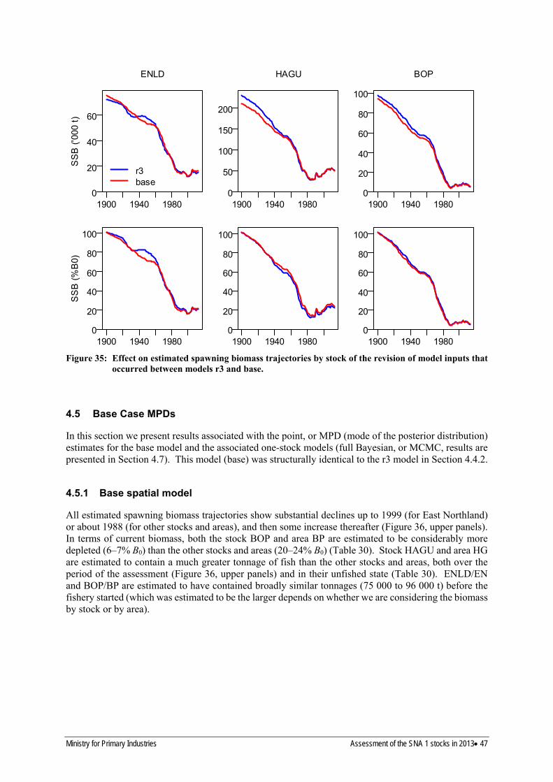
ENLD HAGU BOP

r3 base

200

150

100

50

0

100

80

60

40

20

0

SS

B (

%B

0)

SS

B (

'000

t) 60

40

20

0 1900 1940 1980 1900 1940 1980 1900 1940 1980

100

80

60

40

20

0

100

80

60

40

20

0

100

80

60

40

20

0 1900 1940 1980 1900 1940 1980 1900 1940 1980

Figure 35: Effect on estimated spawning biomass trajectories by stock of the revision of model inputs that occurred between models r3 and base.

4.5 Base Case MPDs

In this section we present results associated with the point, or MPD (mode of the posterior distribution) estimates for the base model and the associated one-stock models (full Bayesian, or MCMC, results are presented in Section 4.7). This model (base) was structurally identical to the r3 model in Section 4.4.2.

4.5.1 Base spatial model

All estimated spawning biomass trajectories show substantial declines up to 1999 (for East Northland) or about 1988 (for other stocks and areas), and then some increase thereafter (Figure 36, upper panels). In terms of current biomass, both the stock BOP and area BP are estimated to be considerably more depleted (6–7% B0) than the other stocks and areas (20–24% B0) (Table 30). Stock HAGU and area HG are estimated to contain a much greater tonnage of fish than the other stocks and areas, both over the period of the assessment (Figure 36, upper panels) and in their unfished state (Table 30). ENLD/EN and BOP/BP are estimated to have contained broadly similar tonnages (75 000 to 96 000 t) before the fishery started (which was estimated to be the larger depends on whether we are considering the biomass by stock or by area).


ENLD or EN HAGU or HG BOP or BP S

SB

(%

B0)

S

SB

('0

00 t

)

bystock byarea

200 80 80

60 150 60

100 40 40

5020 20

0 0 0 1900 1940 1980 1900 1940 1980 1900 1940 1980

100 100 100

80 80 80

60 60 60

40 40 40

20 20 20

0 0 0 1900 1940 1980 1900 1940 1980 1900 1940 1980

Figure 36: Base case estimates of spawning biomass (SSB) by stock (blue lines, for stocks ENLD, HAGU, BOP) and by area (red lines, for areas EN, HG, BP). These are presented in tonnes (upper panels) and relative to the corresponding unfished biomass, B0 (lower panels).

Table 30: Base case estimates of unfished biomass, B0, and current biomass by stock and area. B0 (‘000 t) Bcurrent (%B0)

Stock/area by stock by area by stock by area ENLD/EN 75 88 22 20 HAGU/HG 208 213 24 21 BOP/BP 93 76 6 7

The majority of fish do not move away from their home grounds, with migration being most common for BOP fish, 21% of which migrate to area HG (Table 31).

Table 31: Base case migration matrix (showing proportions of each stock migrating to each area in time step 2).

Area Stock EN HG BP ENLD 0.95 0.04 0.01 HAGU 0.05 0.91 0.03 BOP 0.07 0.21 0.72

Most estimated year-class strengths (YCSs) are between half and double the strength predicted by the stock-recruit relationship (Figure 37).


ENLD HAGU BOP

Tru

e Y

CS

A

ctua

l YC

S

2.5

2.0

1.5

1.0

0.5

0.0

2.5

2.0

1.5

1.0

0.5

0.0

2.5

2.0

1.5

1.0

0.5

0.0 1950 1970 1990 1950 1970 1990 1950 1970 1990

2.0

1.5

1.0

0.5

0.0

2.0

1.5

1.0

0.5

0.0

2.0

1.5

1.0

0.5

0.0 1950 1970 1990 1950 1970 1990 1950 1970 1990

Figure 37: Base case estimates of year-class strengths (YCS) by stock, plotted both as ‘actual’ YCSs (upper panels, where a value of 1 corresponds to the recruitment predicted by the stock-recruit curve) and ‘true’ YCSs (lower panels, where a value of 1 corresponds to the mean unfished recruitment).

The base model fitted reasonably well all the relative and absolute biomass observations (Figure 38). As found in the 2012 assessment model (see Section 3.2) the fit to the tag-recapture data was negatively affected by the conflict between these data and the age compositions. The conflict caused an imbalance in the fits to the tag-recapture data with the observed tag rate (the proportion of fish with tags) greater than the expected rate in 23 of the 26 data sets. Nevertheless, the expected rate lay within the 95% confidence bounds in all but three data sets (Figure 39). Average fits to the composition data were generally good, although observed length frequencies were consistently more peaked than the expected frequencies (Figure 40). Observed trends in mean length and age were reasonably matched by the model (Figure 41).

Estimated exploitation rates varied widely by fishery and were highest in area BP (Figure 42). The estimated selectivities suggested that the research trawl caught the smallest fish and longlines caught the largest (Figure 43).


o oooo o

oooooooooo

o o o

oo ooo oo

o o oooo

o o oo

oo o ooo

o

1980 1990 2000 2010 0.0

0.5

1.0

1.5

BP_STcpue

o

o oo

oo

o

1980 1990 2000 2010 0.0

0.5

1.0

1.5

BP_LLcpue

oo o

oo

o oo

oo o

o

o

1980 1990 2000 2010 0.0

0.5

1.0

1.5

EN_LLcpue

1.5

HG_LLcpue

40

HG_RES_abund

10000

12000 BP_Tag_bio

000

t) a

bund

ance

Rel

ativ

e or

abs

olut

e ('

0.5

oo o o oo o o oo

oooooo oo

ooooo

1980 1990 2000 2010

1.0

10 o o o

o o o

o o

o

o

o

o o

1980 1990 2000 2010

20

800030 o

2000

4000

6000

x

1980 1990 2000 2010 0.0 0 0

Figure 38: Base-case fits (red lines or ‘×’) to relative and absolute biomass observations (‘o’, with 95% confidence intervals as vertical lines).

x ox oEN_EN x x o o

Loca

tion

of f

ish:

rec

aptu

re_t

aggi

ng HG_EN oxoxxox o

BP_EN ooxx

EN_HG xoox xox o

HG_HG x o x oxx o o

BP_HG ox ox

EN_BP xoox

BP_BP

HG_BP oxx o

o o xx

1985 1986 1994 1995

0 2 4 6 8

Observed (o) and expected (x) number tagged per 10 000 scanned

Figure 39: Base-case fits to tag recapture observations. A total of 26 observed values (‘o’, with 95% confidence intervals indicated by horizontal lines) are plotted: these are grouped vertically by their locations of recapture and tagging (with each group identified by the label on the vertical axis – e.g., BP_BP, HG_BP), with the year of recapture (1985, 1986, 1994, or 1995) indicated by the colour of the plotting symbol.


x

x

x

x x x

x x

x x x x x x x x x

x

5 10 15 20 0.00

0.05

0.10

0.15

18 years

x x

x

x x

x x

x

x

x x

x x x x x x

x

0.00

0.05

0.10

0.15

22 years

x

x

x

x

x x

x

x x

x x x x x x0.00

0.05

0.10

0.15

0.20

19 years

x x x

x

x x

x

x x x

x x x x x

x

0.05

0.10

0.15

11 years

x

x

x

x

x x

x 0.1

0.2

0.3

0.4

1 year

EN HG BP

xx x

5 10 15 20 5 10 15 20

RE

C_l

en_p

ost9

5 R

EC

_len

_pre

95

RE

S_a

ge

ST

_age

D

S_a

ge

LL_a

ge

x

5 10 15 20 0.00 x x x x x x x x x x

5 10 15 20 0.0

x x

x

x

x x x x

x x x x x x x x x

x

5 10 15 20 0.00

0.05

0.10

0.15

0.20

0.25

6 years

x

x

x x

x x x x x x x x x x x x x x0.00

0.05

0.10

0.15

0.20

0.25

0.30 4 years

x

x

x

x

x

x

x x

x

x x x x x x x x x x

x 0.00

0.05

0.10

0.15

1 year

x

x x

x x

x

x x x x x x x x x x x x x x0.00

0.05

0.10

0.15

0.20

10 years

x

x

x

x

x

x x

x x x x x x x x x x x x x0.00

0.05

0.10

0.15

0.20

3 years

Mea

n pr

opor

tion

at a

ge/le

ngth

5 10 15 20

0.25

5 10 15 20 5 10 15 20 5 10 15 20

xxxxxxxxxx xx x

x

x

x x x

xx x

xxx

x

x

x x xxxxxxxxxxxxxxxxxxxxxxxxxxxxxxxxxxxxxx0.00

0.02

0.04

0.06

0.08

2 years

xxxxxxxxxxxxx x

x

x

x xx xx

xx x xx xxx

x x xxxxxxxxxxxxxxxxxxxxxxxxxxxxxxxxxxx0.00

0.02

0.04

0.06

0.08

2 years

xxxxxxxxxxxxx x

x

x

x xx

x x

x

x x

xx xxxxxxxxxxxxxxxxxxxxxxxxxxxxxxxxxxxxxxxx0.00

0.02

0.04

0.06

0.08

0.10

0.12 2 years

10 20 30 40 50 60 70 10 20 30 40 50 60 70 10 20 30 40 50 60 70

Age or length Figure 40: Fits to age and length composition data: observed (‘×’) and expected (line) proportions at

age/length averaged across years. The number of years in each data set is given above each panel.

10 20 30 40 50 60 70 10 20 30 40 50 60 70 10 20 30 40 50 60 70

xxxxxxxxxxxxxxxx x

x

x

x

x

xx x x xx

xx xx xxxxxxxxxxxxxxxxxxxxxxxxxxxxxxxxxxx0.00

0.02

0.04

0.06

0.08

12 years

xxxxxxxxxxxxxxxx x

x

x

xx xx

xx

xx

xx xx xx xxxxxxxxxxxxxxxxxxxxxxxxxxxxxxxxx0.00

0.02

0.04

0.06

0.08

12 years

xxxxxxxxxxxxxxxx x

x

x x x

x x

x x xx xx xx xx

xxxxxxxxxxxxxxxxxxxxxxxxxxxx0.00

0.02

0.04

0.06

0.08

0.10

12 years


xxxxx

EN HG BP

Mea

n le

ngth

40REC

40 40

35 35 35

30 30 30

25 25 25

1990 2000 2010 1990 2000 2010 1990 2000 2010

5

10

15

20 LL ST DS RES

5

10

20

5

10

20

Mea

n a

ge 15 15

1970 1990 2010 1970 1990 2010 1970 1990 2010

Figure 41: Base-case fits to mean length (upper panels) and age (lower panels) from the composition observations. The observed means are plotted as short horizontal lines, with their 95% confidence intervals shown as a vertical line; the expected means are plotted as a curved line (or, for data sets with only one year, as an ‘×’). The data sources are identified by colour (REC = recreational; LL = longline; ST = single trawl; DS = Danish seine; RES = research trawl).

1900 1940 1980 0.00

0.05

0.10

0.15

0.20

0.25

0.30 LL ST DS REC PT

1900 1940 1980 0.00

0.05

0.10

0.15

0.20

0.25

0.30

1900 1940 1980 0.00

0.05

0.10

0.15

0.20

0.25

0.30

1900 1940 1980 0.0

0.1

0.2

0.3

0.4

0.5

1900 1940 1980 0.0

0.1

0.2

0.3

0.4

0.5

1900 1940 1980 0.0

0.1

0.2

0.3

0.4

0.5

Exp

loita

tion

rate

EN HG BP

By

fishe

ryB

y ar

ea

Figure 42: Base case estimates of exploitation rates by fishery (upper panels) and by area (lower panels).


1.0

0.8

0.6

0.4

0.2

0.0

Age (y)

RES ST REC_pre95 DS REC_post95 LL

0 5 10 15 20

Pro

port

ion

sele

cted

Figure 43: Selectivities estimated in the base model.

4.5.2 Comparisons with one-stock models

The biomass trajectories estimated from the one-stock models were quite similar to those from the base model (Figure 44), particularly when we focus on the years for which biomass indices were available and consider the trends in biomass, rather than their absolute values (Figure 45). The one-stock models fitted the biomass indices slightly worse than did the base model (Figure 46).

1900 1940 1980 0

20

40

60

80


1900 1940 1980 0

50

100

150

200

1900 1940 1980 0

20

40

60

80

100

SS

B (

'000

t)

1900 1940 1980 0

20

40

60

80

100

1900 1940 1980 0

20

40

60

80

100

1900 1940 1980 0

20

40

60

80

100

SS

B (

%B

0)


Figure 44: Comparison of spawning biomass (SSB) trajectories from the base model (red line, by stock; and blue lines, by area) with those for the corresponding one-stock models (black lines).


Figure 45: Comparison like that in the upper panels of Figure 44 but (a) restricted to the years where there are biomass indices, and (b) with the blue and black lines in each panel scaled to have the same mean as the red line (so as to facilitate the comparison of trend, rather than absolute value).

1990 2000 2010 0

5

10

15


1990 2000 2010 0

10

20

30

40

50

1990 2000 2010 0

2

4

6

8

SS

B (

'000

t)


1.5

HG_LLcpue: -1

4e+07

HG_RES_abund: -1

1.5

EN_LLcpue: 1

0.0 0e+00

o o o

o o o

o o

o

o

o

o o

1980 1990 2000 2010

1e+07

2e+07

3e+07

0.0

BP_STcpue: -5 BP_LLcpue: -5 BP_Tag_bio: -3

oo o o oo

o o oo

oooooo

oo ooo

oo

1980 1990 2000 2010

0.5

1.0

base one-stock

o oo

ooo oo

ooo o oo

ooo o oo

o o o

1980 1990 2000 2010

0.5

1.0

Rel

ativ

e or

abs

olut

e ('0

00 t

) ab

unda

nce

1.5

o o oooo

o o oo

oo o

ooo o

1980 1990 2000 2010

1.0

15000 1.5

o o o oo

oooooooo

ooo oo

ooo oo

1980 1990 2000 2010

1.0

o5000

10000 x

x

1980 1990 2000 2010

0.5 0.5

0.0 0.0 0

Figure 46: Comparison of the fits to the biomass indices from the base model (blue lines) and the corresponding one-stock model (red line). The observations are plotted as ‘o’, with the 95% confidence interval shown as a vertical line. The number shown above each panel on the right is the gain in fit (a negative number means that the one-stock model fitted worse than the base model).


4.6 Sensitivity Analyses

A series of variants of the base model were constructed to determine the sensitivity of this model to various assumptions. They extend the sensitivity analyses described in Section 4.4 and fall into two groups: the main sensitivity runs, which help us to understand the extent of uncertainty in the assessment results; and some additional sensitivity runs, which do not produce credible alternative assessments, but do help us understand the influence of different data sets on the assessment.

4.6.1 Main sensitivity runs

Most of the alternative models in the main sensitivity runs are easily understood from their descriptions in Table 32, but one – reweight – requires more detail. In this run the sample sizes for the age composition data were divided by ten to down-weight these data, and the tag-recapture data were up-weighted by decreasing the associated dispersion parameter from 6.3 to 0.1. This reweighting substantially reduced the imbalance in the fits to the tag-recapture data, with the number of data sets in which the observed recaptures exceeded the expected recaptures being reduced from 23 of 26 to 15 of 26.

Table 32: Brief descriptions of alternative models run to determine sensitivity to various model assumptions.

Label Description catch-lo/hi Use alternative lower and higher catch histories (as in Figure 47) sel-by-area1 Assume that fishery selectivity depends on area, as well as fishing method (corresponds to run r3.sel

in Section 4.4.6) reweight Age and tag-recapture data reweighted to reduce the imbalance in the fit to the tag-recapture data base60 Maximum age in the model partition increased from 20 y to 60 y. M-lo/hi Replace the assumed value of natural mortality, M = 0.075 y-1, with lower (0.05) and higher (0.10)

values steep-lo/hi Replace the assumed value of stock-recruit steepness, 0.85, with lower (0.7) and higher (0.95) values one-stock1 Replace the base three-stock (and three-area) model with 3 separate one-stock models: one for each

area 1MCMC runs were done for these sensitivity runs

Results of the main sensitivity runs are presented in terms of their effects on current status (Figure 48). Regardless of whether this status was measured by stock or by area, all models estimated the Bay of Plenty spawning biomass to be the most depleted, and most estimated that the Hauraki Gulf was least depleted. The greatest sensitivity was shown with two alternative models (discussed in more detail in Section 4.6.3): sel-by-area, which estimated much less depletion for the Bay of Plenty (current biomass was 14%B0, compared to 6–7%B0 in the base model), and reweight, which estimated higher depletion for the other areas. Estimates from sel-by-area were broadly similar to those from the one-stock models. Changes in both M and steepness had predictable effects (the same for all stocks and areas): lower values of these parameters, which imply lower productivity, led to more depletion, and higher values to less depletion. Current status estimates were not very sensitive to either the alternative catch histories or to changing the maximum age in the partition. Stock status was always slightly worse by stock than by area for Bay of Plenty, with the reverse being true for East Northland and Hauraki Gulf.


EN

1900 1920 1940 1960 1980 2000 0 1 2 3 4 5

hi base lo

HG

Cat

ch (

'000

t)

0

2

4

6

8

1900 1920 1940 1960 1980 2000

1900 1920 1940 1960 1980 2000 0 1 2 3 4 5

BP

Figure 47: Comparison of the catch histories by area for the base model with those of sensitivities catch-lo and catch-hi.

By stock By area base

catch-lo catch-hi

sel-by-area reweight base60

M-lo M-hi

steep-lo steep-hi

onestock

E E E E

E E

E E

E E E

H H

H H

H H

H H

H H

H

B B B

B B

B B

B B

B B

+ +

+ +

+ +

+ +

+ +

+

ENLD E HAGU H

BOP B HGBP +

E E

E E

E E

E E

E E

E

H H

H H

H H

H H

H H

H

B B

B B

B B B

B B B

B

+ +

+ +

+ +

+ +

+ +

+

0 10 20 30 40 0 10 20 30 40

Current status (Bcurrent as %B0) Figure 48: MPD estimates of current status (B2013 as %B0), by stock and area, for the base model and some

sensitivity analyses. The horizontal broken line separates the one-stock estimates from the others as a reminder that there is no distinction between spawning biomass by stock and by area for these models.


4.6.2 Additional sensitivity runs

4.6.2.1 Tagging data sensitivity further exploration

The tagging data was found to be strongly informative on both overall biomass and how this biomass is distributed between stock and areas (movement). The “reweight” sensitivity shows the effect on the assessment when increased weight was placed on the tagging observations. As requested by the Working Group an alternative sensitivity (lowtagwt) was undertaken whereby the tagging data weighting was substantially reduced by dropping the tagging biomass observation, BP_Tag_bio, and multiplying the tag-recapture dispersion parameter by 100. The purpose of this extreme down weighting was an attempt to “neutralise” the biomass signal while still allowing the tag data to inform the model on movement.

As also shown in Figure 48, increasing the weight on the tagging data (reweight) resulted in lower biomass to B0 ratios for the east Northland and Hauraki Gulf stocks whereas the Bay of Plenty ratios were relative similar (Figure 49). The Bay of Plenty stock status and SSB trajectory was largely unaffected by substantively down weighting the tagging data, whereas the east Northland and Hauraki Gulf stocks showed markedly higher biomass trajectories under down-weighting (Figure 49).

ENLD HAGU BPLE

1900 1960

0 2

0 40

60

80

base lowtagwtreweight

1900 1960

0 5

0

15

0

1900 1960

0

20

6

0

10

0

SS

B (

'00

0 t)

1900 1960

0

20

6

0

10

0

1900 1960

0

20

6

0

10

0

1900 1960

0

20

6

0

10

0

SS

B (

%B

0)

Figure 49: Comparison of spawning biomass trajectories by stock from the two tag weighting sensitivities (reweight, lowtagwt) with those from the base run.

The “base” and “lowtagwt” tag weighting scenarios produced very similar fits to the CPUE indices (relative abundance; Figure 50). Down weighting the tagging data resulted in markedly improved fits to the compositional data but a poorer fit to the CPUE indices (relative abundance; Figure 50). These results are consistent with the sensitivity analysis undertaken using the 2012 assessment model, i.e. the same explanation applies (see Section 3.2).

As a generality, the more tags recovered per unit catch, the lower the predicted biomass. The number of predicted tags expressed as a percentage of observed was highest in the high tag model weighting


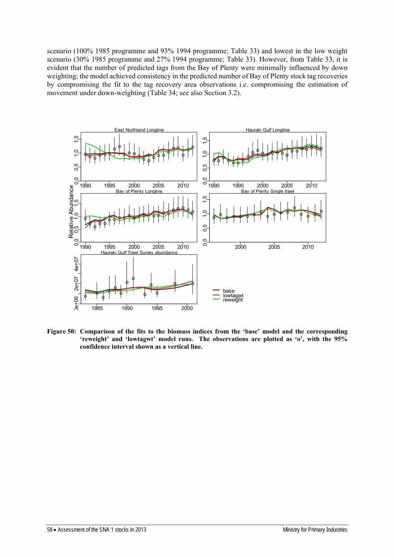
0

0

scenario (100% 1985 programme and 93% 1994 programme; Table 33) and lowest in the low weight scenario (30% 1985 programme and 27% 1994 programme; Table 33). However, from Table 33, it is evident that the number of predicted tags from the Bay of Plenty were minimally influenced by down weighting; the model achieved consistency in the predicted number of Bay of Plenty stock tag recoveries by compromising the fit to the tag recovery area observations i.e. compromising the estimation of movement under down-weighting (Table 34; see also Section 3.2).

Rel

ativ

e A

bund

ance

0e

+00

4e

+07

0.

0 0.

5 1.

0 1.

5 0.

0 0.

5 1.

0 1.

5

o o o o o o

o o

o o o o o o

o o o o o o

o o o

1990 1995 2000 2005 2010

East Northland Longline Hauraki Gulf Longline

0.0

0.5

1.0

1.5

0.0

0.5

1.0

1.5

o o o o o o o o

o o o o o o o o o o

o o o o o

1990 1995 2000 2005 2010

o o o o o o o o

o o o o o

o o o o

o o

o o o

o o o o o o o o o o o o o o o o o o

1990 1995 2000 2005 2010

Bay of Plenty Longline Bay of Plenty Single trawl

2000 2005 2010 Hauraki Gulf Trawl Survey abundance

o72e

+0

o o o o o

o o

o o o o o base

lowtagwt

Figure 50: Comparison of the fits to the biomass indices from the ‘base’ model and the corresponding ‘reweight’ and ‘lowtagwt’ model runs. The observations are plotted as ‘o’, with the 95% confidence interval shown as a vertical line.

reweight

1985 1990 1995 2000


Table 33: Observed and predicted (% of observed) numbers of tag recoveries by stock for each tag weighting scenario.

% predicted of observed recoveries

Stock Observed tags Reweight Base Lowtagwt

1994 tag recoveries

ENLD 144 93% 55% 22%

HAGU 309 94% 55% 18%

BPLE 68 90% 85% 81%

Total 521 93% 59% 27%

1985 tag recoveries

ENLD 447 98% 88% 30%

HAGU 1021 100% 90% 29%

Total 1468 100% 89% 30%

Table 34: Comparison of estimated migration matrices from runs lowtagwt, base and reweight. The tabulated numbers are the proportions of each stock migrating to each area in time step 2.

Lowtagwt Base Area Reweight Stock EN HG BP EN HG BP EN HG BP

ENLD 0.997 0.003 0 0.947 0.044 0.01 0.895 0.044 0.061

HAGU 0.002 0.979 0.02 0.055 0.912 0.032 0.075 0.822 0.103

BOP 0.001 0.004 0.995 0.14 0.186 0.674 0.053 0.298 0.649

4.6.2.2 CPUE sensitivity

To gain an understanding of how influential the CPUE indices were in the assessment a sensitivity analysis was undertaken whereby these indices were replaced by their unstandardized values, which have quite different trends (Figure 51).

EN HG BP1.4

1.5 1.2 1.5

1.0

1.0 0.8 1.0

0.6

0.5 0.4 0.5

0.2

0.0 0.0 0.0

Figure 51: Comparison between the standardised and unstandardized longline CPUE indices in the three areas.

std unstd

1990 2000 2010 1990 2000 2010 1990 2000 2010


A marked change is seen in the biomass trajectories (Figure 52), demonstrating how strongly the assessment results depend on the CPUE data. The Working Group accepted the standardised over the unstandardised CPUE series as indices of abundance hence the ‘unstd’ model was not deemed to be a viable alternative to the ‘base’ model.

ENLD HAGU BPLE

SS

B (

%B

0)

SS

B (

'00

0 t)

0

20

40

60

80

1900 1960

base unstd

1900 1960

0

50

1

50

1900 1960

02

0

60

1

00

1900 1960

02

0

60

1

00

1900 1960

02

0

60

1

00

1900 1960

02

0

60

1

00

Figure 52: Comparison of spawning biomass trajectories between ‘unstd’ (which used unstandardised CPUE) with those from the base run.

4.6.3 Should the base model be changed?

The Working Group seriously considered, but eventually rejected, the possibility of replacing the base model by either sel-by-area or reweight.

In Section 3 it was noted that a key signal in the composition data is the fact that, for a given fishing method in a given year, the mean age of fish caught in area BP was almost always less than that for fish caught in EN or HG (where the data allowed such a comparison) (Figure 12). Because both the base 2012 and 2013 assessment models assume that the selectivity for each fishing method does not depend on area, this signal implies that the biomass is more depleted in BP than in the other areas. In sel-by-area this signal can be (and was) interpreted as evidence that the BP selectivity for each fishing method is shifted to the left of those for the other areas (Figure 53). Thus there is a need to choose between two hypotheses to explain the mean-age signal: either the biomass is more depleted in area BP, or all fishing methods tend to select younger fish in this area than elsewhere. The former hypothesis supports the base model; the latter supports sel-by-area. In this context, one weakness of both models is that all selectivities are age-based, whereas actual selectivities are probably length-based (unfortunately, length-based selectivities – which are available in CASAL – could not be used in either model because of computational constraints). It was thought that the lower mean ages in BP could be a result of faster growth in this area combined with selectivities which are length-based and area-invariant. However, if the biomass were no more depleted in BP than in the other areas this should imply that mean lengths in BP would be similar to those in HG and EN, which was not true: in those combinations of fishing method and year for which a comparison could be made, mean lengths in BP were less than those in EN in 27/31 cases, and less than those in HG in 26/36 cases (Figure 54).


Although the Working Group decided not to adopt sel-by-area as a base model they did not consider it completely implausible. Because of this (together with other uncertainties about the relationship between fish in areas HG and BP) the Working Group decided to describe the status of stocks in SNA 1 in terms of ENLD and HAGUBOP, rather than ENLD, HAGU, and BOP.

LL ST DS 1.0

EN HG BP

1.0 1.0

0.8 0.8 0.8

0.6 0.6 0.6

0.4 0.4 0.4

0.2 0.2 0.2

0.0 0.0 0.0 0 5 10 15 20 0 5 10 15 20 0 5 10 15 20

Pro

port

ion

sele

cted

REC_pre95 REC_post95 RES 1.0 1.0 1.0

0.8 0.8 0.8

0.6 0.6 0.6

0.4 0.4 0.4

0.2 0.2 0.2

0.0 0.0 0.0 0 5 10 15 20 0 5 10 15 20 0 5 10 15 20

Age (y) Figure 53: Selectivities, by fishing method and area, as estimated in model sel-by-area.


LL RES ST

x40 x EN HG

x38 BP x xxx x x x x36 x xx x xx x x xx xx x x xxxxxx

x xxxxx xxx xxx xx xx x34 xx x xxx xx

32 x

xx25 x24

x x23 x x x x22

21 x xx x20

19 x

xx 34.0

33.5

33.0 x x32.5

32.0

31.5 x x31.0 x

1985 1995 2005

31

32

33

34

35

36

37 x

xx x

x

Mea

n le

ngth

(cm

)

1985 1995 2005 1985 1995 2005 1985 1995 2005

DS REC xx

x36 x x x xx xx xxx x xxx x xx xx x34 x xxx x xxx xx x x x

x32 x xx x

30 x

1995 2005

Figure 54: Observed mean length by fishing method and area.

The runs ‘base’ and ‘reweight’ provide a clear example of how the relative weight given to different data sets can have a profound effect on the outcome of an assessment (Figure 49). There were two considerations which led the Working Group to accept the ‘base’ over the ‘reweight’ scenario.

Firstly; although the 1985 and 1994 tagging programmes were acknowledged by the Working Group to be well designed and executed such that the results are “credible”, uncertainties still exist as to the degree of contagion present in these data sets (Gilbert & McKenzie 1999) and hence the programmes may have delivered a higher than “expected” number of tag recoveries. For this reason the Working Group favoured the “base” over “reweight” level of tag weighting, but felt there was sufficient confidence in the tagging data not to accept a poorer than ‘base’ fit to the tagging data, e.g. lowtagwt (Table 33).

Secondly; the model fits to the CPUE series were poorer under high tag weighting (reweight; Figure 50), an observation which was at odds with an important data-weighting principle given by Francis (2011) being “do not let other data stop the model from fitting abundance data well”. Although the tagging data provide a strong absolute biomass signal for 1985 and 1994 fishing years in accordance with Francis (2011) these data should not be accorded sufficient weight to “contradict” the multiple-year abundance trend seen in the CPUE series (Figure 50).

4.7 Base Case Model MCMC Results

For the base model we calculated fully Bayesian estimates by generating twelve MCMC chains of length about 1 million, each starting at a different point (generated by randomly stepping away from the MPD). Following Francis (2005), all parameters that were estimated at a bound in the MPD were fixed in the MCMC in order to improve convergence (there were three such parameters: the parameters controlling the right limb of the LL selectivity [estimated at its upper bound] and the left limbs of both REC selectivities [at their lower bounds]). The chains were concatenated and systematically subsampled to produce final chains of length 3000.


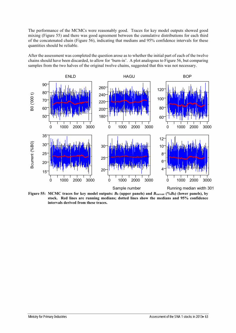
The performance of the MCMCs were reasonably good. Traces for key model outputs showed good mixing (Figure 55) and there was good agreement between the cumulative distributions for each third of the concatenated chain (Figure 56), indicating that medians and 95% confidence intervals for these quantities should be reliable.

After the assessment was completed the question arose as to whether the initial part of each of the twelve chains should have been discarded, to allow for ‘burn-in’. A plot analogous to Figure 56, but comparing samples from the two halves of the original twelve chains, suggested that this was not necessary.

ENLD HAGU BOP

90

80

70

60

50

260

240

220

200

180

120

100

80

60

Bcu

rren

t (%

B0)

B

0 ('0

00 t

)

0 1000 2000 3000 0 1000 2000 3000 0 1000 2000 3000

35

30

25

20

15

30

25

20

12

10

8

6

4

0 1000 2000 3000 0 1000 2000 3000 0 1000 2000 3000

Sample number Running median width 301 Figure 55: MCMC traces for key model outputs: B0 (upper panels) and Bcurrent (%B0) (lower panels), by

stock. Red lines are running medians; dotted lines show the medians and 95% confidence intervals derived from these traces.


C

umul

ativ

e pr

obab

ility

ENLD HAGU BOP

1.0 1.0 1.0

0.8 0.8 0.8

0.6 0.6 0.6

0.4 0.4 0.4

0.2 0.2 0.2

0.0 0.0 0.0

50 60 70 80 90 180 220 260 60 80 100

B0 ('000 t)

1.0

0.8

0.6

0.4

0.2

0.0

1.0

0.8

0.6

0.4

0.2

0.0

1.0

0.8

0.6

0.4

0.2

0.0

15 20 25 30 35 20 25 30 4 6 8 10 12

Bcurrent (%B0)

Figure 56: Diagnostics for MCMC chains. Each panel contains three cumulative probability distributions – one for each third of the concatenated chain – for one of the six key model outputs.

All estimated spawning biomass trajectories show substantial reductions up to 1999 (for East Northland) or about 1988 (for other stocks and areas), and then some increase thereafter (Figure 57, upper panels). In terms of current biomass, both the stock BOP and area BP are estimated to be more depleted (3–10% B0) than the other stocks and areas (15–30% B0), with depletion being worse by stock than by area for Bay of Plenty, and vice versa elsewhere (Table 35). However, for all stocks and areas current biomass is 30–68% higher than the minimum value in the biomass trajectory (Table 35). Stock HAGU and area HG are estimated to contain a much greater tonnage of fish than the other stocks and areas, both over the period of the assessment (Figure 57, upper panels) and in their unfished state (Table 35). ENLD/EN and BOP/BP are estimated to have contained broadly similar tonnages (53 000 to 112 000 t) before the fishery started. No stock or area is at or above the target and none but the Bay of Plenty is below the hard limit. Probabilities of being below the soft limit range from 0.04 to 1.00 (Table 36).


S

SB

(%

B0)

S

SB

('0

00 t

)ENLD or EN HAGU or HG BOP or BP

By stock By area

250 100 100

200 80 80

150 60 60 100 40 40

20 50 20

0 0 0 1900 1960 1900 1960 1900 1960

100 100 100

80 80 80

60 60 60

40 40 40

20 20 20

0 0 0 1900 1960 1900 1960 1900 1960

HAGUBOP or HGBP

0

50

100

150

200

250

300

1900 1960

0

20

40

60

80

100

1900 1960

Figure 57: Spawning biomass (SSB) trajectories by stock (red lines) and area (blue lines) from the base model. Solid lines are MCMC medians, broken lines are 95% confidence intervals.

Table 35: Base model estimates of unfished biomass (B0) and current biomass (B2013 as %B0 and %Bmin) by stock and area. Estimates are MCMC medians with 95% confidence intervals in parentheses.

By stock ENLD HAGU BOP HAGUBOP

By area EN HG BP HGBP

B0 (‘000 t)

66 (53, 79) 220 (192, 246) 86 (63, 112)

306 (288, 325)

96 (85, 111) 211 (197, 227) 64 (53, 74)

276 (258, 292)

B2013 (%B0)

24 (18, 30) 24 (19, 29)

6 (3, 9) 19 (15, 23)

20 (16, 25) 21 (17, 26) 7 (5, 10)

18 (15, 22)

B2013 (%Bmin)1

137 (108, 176) 168 (137, 206) 148 (104, 209) 167 (139, 201)

130 (108, 159) 167 (136, 204) 145 (114, 185) 165 (136, 199)

1Bmin was taken as B1999 for ENLD and EN, and as B1988 for other stocks and areas


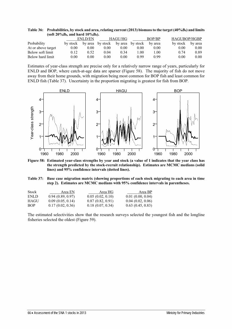
Table 36: Probabilities, by stock and area, relating current (2013) biomass to the target (40%B0) and limits (soft 20%B0, and hard 10%B0).

ENLD/EN HAGU/HG BOP/BP HAGUBOP/HGBP Probability by stock by area by stock by area by stock by area by stock by area At or above target 0.00 0.00 0.00 0.00 0.00 0.00 0.00 0.00 Below soft limit 0.12 0.52 0.04 0.34 1.00 1.00 0.74 0.89 Below hard limit 0.00 0.00 0.00 0.00 0.99 0.99 0.00 0.00

Estimates of year-class strength are precise only for a relatively narrow range of years, particularly for ENLD and BOP, where catch-at-age data are sparser (Figure 58). The majority of fish do not move away from their home grounds, with migration being most common for BOP fish and least common for ENLD fish (Table 37). Uncertainty in the proportion migrating is greatest for fish from BOP.

ENLD HAGU BOP

4 4 4

3 3 3

2 2 2

1 1 1

0 0 0

Figure 58: Estimated year-class strengths by year and stock (a value of 1 indicates that the year class has the strength predicted by the stock-recruit relationship). Estimates are MCMC medians (solid lines) and 95% confidence intervals (dotted lines).

Table 37: Base case migration matrix (showing proportions of each stock migrating to each area in time step 2). Estimates are MCMC medians with 95% confidence intervals in parentheses.

Stock Area EN Area HG Area BP ENLD 0.94 (0.89, 0.97) 0.05 (0.02, 0.10) 0.01 (0.00, 0.04) HAGU 0.09 (0.05, 0.14) 0.87 (0.82, 0.91) 0.04 (0.02, 0.06) BOP 0.17 (0.02, 0.36) 0.18 (0.07, 0.34) 0.63 (0.45, 0.83)

The estimated selectivities show that the research surveys selected the youngest fish and the longline fisheries selected the oldest (Figure 59).

Yea

r-cl

ass

stre

ngth

1960 1980 2000 1960 1980 2000 1960 1980 2000


RES REC_pre95 ST 1.0 1.0 1.0

0.8 0.8 0.8

0.6 0.6 0.6

0.4 0.4 0.4

0.2 0.2 0.2

0.0 0.0 0.0

Pro

port

ion

sele

cted

0 5 10 15 20 0 5 10 15 20 0 5 10 15 20

DS REC_post95 LL 1.0 1.0 1.0

0.8 0.8 0.8

0.6 0.6 0.6

0.4 0.4 0.4

0.2 0.2 0.2

0.0 0.0 0.0

0 5 10 15 20 0 5 10 15 20 0 5 10 15 20

Age (y) Figure 59: MCMC estimates of selectivities (solid lines are medians; dotted lines are 95% confidence

intervals).

4.8 Five-year Projections

Five-year projections were carried out under ‘status quo’ conditions, which were taken to mean constant catches (equal to the 2012 and 2013 catches) for the commercial fisheries and constant exploitation rate (equal to the average of the 2008–2012 rates) for the recreational fisheries.

Projections also required specifying future growth rates and future year class strengths (YCS). To accommodate time varying growth (see Section 2.3) growth was specified in the model using length at-age matrices (see Section 4.2.1), consequently the model B0 is likely to be based on an “ averaged” rate of the growth from these matrices; it is therefore not obvious what growth rate to assume in the model projections. An assumed future growth rate lower than the model implied B0 “average” will result in a mean future productivity lower than B0 i.e. B0 will never be attained even under zero fishing. Uncertainty in future YCS were introduced in the projections by randomly resampling the model YCS estimated deviates; by definition the mean of all the unscaled model YCS deviates will be 1. However when a subset of the available YCS deviates are used in the projections instead of the full range, their average may not equal 1; thus mean future productivity will either be above or below B0 depending on the bias.

Given that the projections were intended to reflect the “likely” trajectory of the stock over the proceeding five years, the Working Group opted to assume:

1. Future growth will be at 2006–2010 average (lower growth rates); 2. Simulated year-class strengths (YCSs) resampled from the 10 most recent reliably estimated

YCSs (deemed to be 1995–2004). Note: the simulated YCSs included both the recent YCSs that were not estimated (because of lack of recent age composition data) in the MPD (2008– 2012) as well as the five “future” YCSs (2013–2017).

Projections also require the additional assumption that relative recreational catchability will remain at the values that were associated with the projected exploitation rate. The Working Group agreed to test



2013 2015 2017 2013 2015 2017 2013 2015 2017 2013 2015 2017

Figure 60: Projected spawning-stock biomass (SSB) by stock and by area. Estimates are MCMC medians (solid lines) and 95% confidence intervals (broken lines). Black lines are projections using only the 10 most recent YCS (i.e. YCS variations higher than mean recruitment); grey lines are projections where all estimable YCS were used (i.e. YCS variations around mean recruitment).

With status quo fishing the biomass in 2018 is very unlikely to be at or above the target for any area or stock; but probabilities relating to the soft and hard limits depend strongly on stock and or area (Table 38).

The predicted future status of the stocks in 2018 were less optimistic when projections were undertaken resampling from all model YCS deviates (grey lines Figure 60; Table 38). The decision as to which of these two projections should be given the greater credence depends on a subjective choice between two possible future recruitment patterns: above average or average. The Working Group felt that recruitment variability over the projection period to 2018 was more likely to be similar to that of the preceding 10 years (i.e. above average) and placed greater emphasis on that projection outcome.

0 5

10

15

20

25

0 5

10

15

20

25

30SS

B (

%B

0)

30

0

2013 2015 2017 2013 2015 2017 2013 2015 2017 2013 2015 2017

EN HG BP HGBP

5 10

15

20

25

30

35

YCS-950 YCS-all

ENLD HAGU

0 2

4 6

8 10

12

0 5

10

15

20

25

30

35

0 2

4 6

8 10

12

0 5

10

15

20

25

0 5

10

15

20

25

by

are

a

by

sto

ck

the sensitivity of the projections to the catchability assumption by projecting forward using high and low recreational exploitation rate estimates: a) from 2013, the final model year, and b) from the average 1995–2005 exploitation rate, a period of relatively constant recreational catch incorporating the 2005 aerial catch estimate.

With status quo catches the biomass is likely to increase for all stocks and areas (Figure 60 black lines). These results changed only slightly when the future exploitation rate for the recreational fishery in HG was changed from 0.0779 (the average of the 2008–2012 rates) to 0.0648 (the average for 1995–2005) or 0.1089 (the rate for 2013). Projections from the one-stock and sel-by-area sensitivity models predicted increasing or near-stable biomass for all stocks and areas.

BOP HAGUBOP

Table 38: Projection comparisons: recent (95 – 04) resampling to where all YCS are resampled. Stock status probabilities, by stock and area, relating the biomass in 2018 after status quo projections to the target (40%B0) and limits (soft 20%B0, and hard 10%B0).

ENLD/EN HAGU/HG BOP/BP HAGUBOP/HGBP Probability by stock by area by stock by area by stock by area by stock by area YCS 95 -04 At or above target 0.01 0.00 0.00 0.00 0.00 0.00 0.00 0.00 Below soft limit 0.06 0.22 0.02 0.11 1.00 1.00 0.35 0.46 Below hard limit 0.00 0.00 0.00 0.00 0.92 0.84 0.00 0.00

YCS All estimated At or above target 0.00 0.00 0.00 0.00 0.00 0.00 0.00 0.00 Below soft limit 0.10 0.53 0.31 0.62 1.00 1.00 0.88 0.93 Below hard limit 0.00 0.00 0.00 0.00 0.99 0.99 0.00 0.00

4.9 Deterministic BMSY and Fishing Intensity

Deterministic BMSY was calculated (using the same method as in Francis & McKenzie (2015), illustrated in Figure 61) as 25–26% B0 for all individual stocks and areas, and 30% for the combined Hauraki Gulf/Bay of Plenty (Table 39).

Table 39: Estimates of deterministic BMSY (%B0) by stock (ENLD, HAGU, BOP, or HAGUBOP) and by area (EN, HG, BP, or HGBP).

ENLD HAGU BOP HAGUBOP By stock 26 26 26 30 By area 26 25 25 30

There are several reasons why BMSY, as calculated in this way, is not a suitable target for management of the SNA 1 fishery. First, it assumes a harvest strategy that is unrealistic in that it involves perfect knowledge (including perfect catch and biological information and perfect stock assessments [because current biomass must be known exactly in order to calculate target catch]), a constant-exploitation management strategy with annual changes in TACs (which are unlikely to happen in New Zealand and not desirable for most stakeholders), and perfect management implementation of the TAC and catch splits with no under- or overruns. Second, it assumes perfect knowledge of the stock-recruit relationship, which is actually very poorly known. Third, it would be very difficult with such a low biomass target to avoid the biomass occasionally falling below 20% B0, the default soft limit according to the Harvest Strategy Standard. Thus, the actual target needs to be above this theoretical optimum; but the extent to which it needs to be above has not been determined.


ENLD HAGU BOP HAGUBOP

0

1

2

3

4

5 by stock by area

0

1

2

3

4

5

0

1

2

3

4

5

0

1

2

3

4

5

Equ

ilibr

ium

cat

ch (

'000

t)

0.0 0.4 0.8 0.0 0.4 0.8 0.0 0.4 0.8 0.0 0.4 0.8

Equ

ilibr

ium

SS

B (

%B

0) 100

80

60

40

20

0 0

20

40

60

80

100 100

80

60

40

20

0

100

80

60

40

20

0 0.0 0.4 0.8 0.0 0.4 0.8 0.0 0.4 0.8 0.0 0.4 0.8

Exploitation rate multiplier, Umult Figure 61: Illustration of the method for estimating deterministic BMSY by stock (red lines) and by area

(blue lines). The plotted lines show the equilibrium catch (upper panels) and spawning biomass (lower panels) that would be achieved with deterministic recruitment and a level of fishing that is a given multiple, Umult, of 2013 exploitation rates. The broken lines show how BMSY is determined from these plots: for area HG these lines in the upper panel show that equilibrium catch is maximised at Umult = 0.75; in the lower panel they show that the equilibrium SSB for this value of Umult is 25% B0.

Results from the deterministic BMSY calculations were used to determine the level of fishing that would maintain the spawning biomass at the interim target level of 40%B0. This ranged from 19% to 59% of the 2013 level (Table 40).

Table 40: Estimated levels of fishing – expressed as multiples of 2013 exploitation rates – that would be required to maintain spawning biomass at 40%B0.

ENLD HAGU BOP HAGUBOP By stock 0.59 0.50 0.19 0.38 By area 0.55 0.46 0.21 0.38

For management purposes it may be more useful to provide exploitation rates by stock (rather than by fishery or area, as given in Figure 42). These are not standard CASAL ouput but were calculated as

a, f, s, and y index age, fishery, stock and year, C is the , where subscripts ൯௦௬ܰ⁄௦௬ܥ ∑൫max ൌ௦௬ܷcatch in numbers, and N is the number of fish in the population immediately before the first fishery of the year. Fishing intensity was estimated to be highest in BOP, and for ENLD and HAGU it has declined from its peak in the 1980s (Figure 62).


ENLD HAGU BOP HAGUBOP F

ishi

ng in

tens

ity

0.4 0.4 0.4 0.4

0.3 0.3 0.3 0.3

0.2 0.2 0.2 0.2

0.1 0.1 0.1 0.1

0.0 0.0 0.0 0.0 1900 1960 1900 1960 1900 1960 1900 1960

Figure 62: MPD estimates of fishing intensity by year and stock. Broken lines show the intensity required to maintain the spawning biomass at 40%B0 (for each panel this was calculated by multiplying the 2013 estimate of fishing intensity by the appropriate multiplier from Table 40).


5 DISCUSSION

In this assessment we have overcome the two major weaknesses identified by Francis & McKenzie (2015) in the 2012 assessment – poor estimation of initial depletion (Rinitial) and poor MCMC diagnostics – and developed an assessment which, despite some uncertainties, provides useful stock status information for fishery managers.

The major uncertainties relate to three key assumptions (see Table 15 and associated text), the correct weighting of different data sets, and the significance of lower observed mean lengths in area BP (these last two issues are discussed in Section 4.6.3). Various other uncertainties (e.g., effect of changing trap-shyness or tag-loss rates, or the maximum age in the partition) have been reduced by the analyses described in Sections 4.4, 4.5and 4.6.

The long time series of catch at-age observations provides evidence for the existence of at least three SNA 1 stocks. The tagging data indicates that some interchange occurs between all three stock areas. However, the “true” location of stock boundaries, mixing and interchange rates, and area specific gear selectivities are imprecisely known, with more tagging data needed at finer spatial scales to reduce uncertainty in these areas. The current assessment suggests that the Bay of Plenty is highly likely to be below the hard limit of 10% B0, this result is in part based on the fit to 49 (now 20 year old) tag observations; these being the only data the model had to estimate movement from and to the Bay of Plenty. As discussed in Section 4.6.3, the model selectivity assumptions also influenced the Bay of Plenty assessment outcome. There was a paucity of age data to estimate gear selectivity other than longline and recreational line in each of the three stock areas; the scant age data available from Danish seine and trawl methods were over 20 years old. The current assessment represents the most probable (best) interpretation of the available data but its conclusions are somewhat “weakened” by a paucity of observations for estimating movement and selectivity, this being why the Working Group had greater confidence in the combined Hauraki Gulf/Bay of Plenty assessment result than the model results for the two areas separately.

The modelling brought to light conflict between the biomass signal in the tagging data and that in the compositional data; the latter tending to “favour” higher Hauraki Gulf and east Northland stock biomass trajectories. Increasing the weight on the tagging data such that the model generated close to the observed number of tag recoveries, resulted in low predicted stock sizes relative to base and also compromised the fit to the relative abundance indices. The possibility of heterogeneity (contagion) in the tagging data leading to a higher than expected number of tag recoveries was discussed by the Working Group. The Working Group acknowledged that the 1985 and 1994 tagging programmes were generally well designed and well executed given the available knowledge and technology at the time and the results should be accorded reasonable power to inform the assessment. However, the Working Group also acknowledged that the presence of contagion bias in the data cannot be totally discounted. In the base case the model predicted tag recoveries ranged between 60–90% of the observed, it could be reasoned that this differential provides some allowance for contagion bias.

Another concern with the assessment is that the results depend strongly on fishery-dependent data, i.e. the commercial CPUE indices (see Section 4.6.2.2).

A lack of recent catch-at-age data (sampling moved from annual to a three-year catch sampling cycle in SNA 1 after 2009–10) meant that the 2003–04 year class was the most recent “reliably” estimable year-class available for model projections. As a result, the YCSs used for the “base” projections came from a period 8 to 18 years prior to the current model year. Because this period represented a period of above average recruitment, projection scenarios differed markedly from those where the full YCS series was used (see Section 4.8).

The two different projection outcomes seen in Section 4.8 highlight a more generic uncertainty issue concerning future SNA 1 stock status, one of non-stationarity in growth, recruitment and natural mortality, i.e. B0 non-stationarity (see also section 5.5 in Francis & McKenzie 2015). Simply put; if


snapper net productivity (B0) goes up more catch can be taken; net productivity goes down and the amount of surplus production available to all SNA 1 sector groups declines. Ecosystem change is likely to be the main driver of B0 non-stationarity in SNA 1 stocks. There is mounting evidence to suggest that, over the next twenty years, the near shore marine environment on which our coastal snapper fisheries depend will alter in response to climate change and anthropogenic habitat modification; however we largely do not know whether the net effect of environmental change on SNA 1 stock productivity will be positive or negative. It is unlikely that fisheries managers will have much power to prevent or mitigate negative ecosystem effects on SNA 1 stocks. Future SNA 1 management requirements are more likely to be geared toward regulating fishing pressure in light of shifting environmental baselines, if so, more regular stock monitoring (i.e. CPUE, catch at-age, recruitment surveys) and assessments will be required to inform management decisions.

6 ACKNOWLEDGEMENTS

This work was contracted and funded by the Ministry for Primary Industries under research project SNA201101. Bruce Hartill undertook the majority of the analytical work which led to the recreational harvest estimates with John Holdsworth also providing significant input in developing recreational catch histories. Darren Parsons revised and updated the CPUE data series and undertook much of the revised CPUE analyses. Generation of the revised commercial catch history derivation used in the final base model and sensitivity analyses was largely undertaken by Malcolm Francis. Acknowledgement is also due to the Northern Inshore Working Group; the review and recommendations this group provided were critical to the final assessment outcome. Marc Griffiths the Working Group convenor and chair is due special recognition for keeping the assessment process on track. Finally, the authors would like to thank Andy McKenzie and Marc Griffiths for manuscript review and Marianne Vignaux for the final editorial.

7 REFERENCES

Bull, B.; Dunn, A. (2002). Catch-at-age user manual v1.06.2002/09/12. NIWA Internal report 114. 23 p. (Unpublished report held in NIWA library, Wellington.)

Bull, B.; Francis, R.I.C.C.; Dunn, A.; McKenzie, A.; Gilbert, D.J.; Smith, M.H.; Bian, R. (2012). CASAL (C++ algorithmic stock assessment laboratory): CASAL User Manual v2.30-2012/03/21. NIWA Technical Report 135. 280 p.

Crossland, J (1976). Snapper Tagging in North-east New Zealand, 1974: Analysis of Methods, Return Rates, and Movements New Zealand Journal of Marine and Freshwater Research 10 (4) : 675– 86

Davies, N.M. (1999). Assessment of the SNA 1 and SNA 8 stocks for the 1997–98 fishing year. New Zealand Fisheries Assessment Research Document 99/19. 87. p. (Unpublished report held in NIWA library, Wellington.)

Davies, N.M.; Walsh, C. (1995). Length and age composition of commercial snapper landings in the Auckland Fishery Management Area, 1988–94. New Zealand Fisheries Data Report No. 58. 15 p.

Francis, R.I.C.C. (2005). Assessment of hoki (Macruronus novaezelandiae) in 2004. New Zealand Fisheries Assessment Report 2005/35. 97 p.

Francis, R.I.C.C. (2011). Data weighting in statistical fisheries stock assessment models. Canadian Journal of Fisheries and Aquatic Sciences 68: 1124–1138.

Francis, R.I.C.C.; McKenzie, J.R. (2015). Assessment of the SNA 1 stocks in 2012. New Zealand Fisheries Assessment Report 2015/xx.

Gilbert, D.J.; McKenzie, J.R. (1999). Sources of bias in biomass estimates from tagging programmes in the SNA 1 snapper (Pagrus auratus) stock. New Zealand Fisheries Assessment Research Document 99/16. 47. p. (Unpublished report held in NIWA library, Wellington.)

Gilbert, D.J.; McKenzie, J.R.; Davies, N.M.; Field, K.D. (2000). Assessment of the SNA 1 stocks for the 1999–2000 fishing year. New Zealand Fisheries Assessment Report 2000/38. 52 p.


Gilbert, D.J.; Sullivan, K.J.; Davies, N.M.; McKenzie, J.R.; Francis, M.P.; Starr, P.J. (1996). Population modelling of the SNA 1 stock for the 1995–96 fishing year. New Zealand Fisheries Assessment Research Document 96/15 39 p. (Unpublished document held in NIWA library, Wellington.)

Hartill, B.; Bian, R.; Armiger, H.; Vaughan, M.; Rush, N. (2007). Recreational marine harvest estimates of snapper, kahawai, and kingfish in QMA 1 in 2004–05. New Zealand Fisheries Assessment Report 2007/26. 44 p.

Hartill, B.; Bian, R.; Rush, N.; Armiger, H. (2013). Aerial-access recreational harvest estimates for snapper, kahawai, red gurnard, tarakihi and trevally in FMA 1 in 2011–12. New Zealand Fisheries Assessment Report 2013/07 44 p.

Hilborn, R.; Stokes, K. (2010). Defining Overfished Stocks: Have we lost the Plot? Fisheries, Vol 35:113–120.

Holdsworth, J.C.; Boyd, R.O. (2008). Size, condition and estimated release mortality of snapper (Pagrus auratus) caught in the SNA 1 recreational fishery, 2006–07. New Zealand Fisheries Assessment Report 2008/53. 37 p.

King, M.R. (1985). Fish and shellfish landings by domestic fishermen, 1974–82. Fisheries Research Division Occasional Publication: Data Series 20. 96 p.

King, M.R.; Jones, D.M.; Fisher, K.A.; Sanders, B.M. (1987). Catch statistics for foreign and domestic commercial fishing in New Zealand waters, January - December 1984 New Zealand Fisheries Data Report 30. 150 p.

McKenzie J.R. (2000). Factors Affecting Mortality of small Snapper (Pagrus auratus) caught and released by the SNA 1 Longline Fishery. Draft Fisheries Assessment Report (held NIWA Library Wellington).

McKenzie, J.R. (2012). An evaluation of age-structured spatially disaggregated stock assessment models for SNA 1. New Zealand Fisheries Assessment Report 2012/38. 76 p.

McKenzie, J.R.; Davies, N.M. (1996). 1994 Recruited biomass Estimation of the east coast North Island Snapper stock (SNA 1) by Petersen mark recapture. (Unpublished contract report for the Ministry of Fisheries held by NIWA Library Wellington.)

McKenzie, J.R.; Parsons, D.M. (2012). Fishery characterisations and catch-per-unit-effort indices for three sub-stocks of snapper SNA 1, 1989–90 to 2009–10. New Zealand Fisheries Assessment Report 2012/29. 112 p.

Millar, R.B.; Akroyd, J.M.; Walshe, K.A.R. (2001). Incidental mortality of snapper in SNA 1 and SNA 8. New Zealand Fisheries Assessment Report 2001/78. 36 p.

Ministry of Fisheries (2008). Harvest Strategy Standard for New Zealand Fisheries. (Unpublished document held by Ministry for Primary Industries.)

Paul, L.J. (1977). The commercial fishery for snapper Chrysophrys (Pagrus) auratus in the Auckland region, New Zealand, from 1900 to 1971. Fisheries Research Division Bulletin, No 15. 84 p.

Paul, L.J.; Sullivan, K.J. (1988). Snapper. New Zealand Fisheries Assessment Research Document 88/26. (Unpublished document held by NIWA library, Wellington.)

Ritchie, L.; Saul, P.; O'Sullivan, K. (1975). The wetfish report 1941–1970. New Zealand Ministry of Agriculture and Fisheries Fisheries Technical Report 137. 370 p.

Smith, I.W.G. (2011). Estimating the magnitude of pre-European Maori marine harvest in two New Zealand study areas. New Zealand Aquatic Environment and Biodiversity Report No. 82.

Sullivan, K.J. (1985). Snapper. In: Colman, J.A.; McKoy, J.L.; Baird, G.G. Background papers for the 1985 Total Allowable Catch recommendations. Fisheries Research Division, New Zealand Ministry of Agriculture and Fisheries. 259 p. (Unpublished report held in NIWA library, Wellington.)

Sullivan K.J.; Hore A.J.; Wilkinson, V.H. (1988). Snapper. In: Baird, G.G.; McKoy, J.L. Papers from the workshop to review fish stock assessments for the 1987–88 New Zealand Fishing Year. 300 p. (Preliminary discussion paper, held in NIWA library, Wellington.)

Walsh, C.; McKenzie, J.; Buckthought, D.; Armiger, H.; Ferguson, H.; Smith, M.; Spong, K.; Miller, A. (2011). Age composition of commercial snapper landings in SNA 1, 2009–10. New Zealand Fisheries Assessment Report 2011/54.


8 APPENDICES

Appendix 1: A new theory for properly weighting tag-recapture data

In the ith length bin of the jth tag-recapture observation (in which both recaptures and numbers scanned are by length), let

Nij be the number of fish scanned

nij be the actual number of tags recovered

mij be the expected number of tags recovered

The likelihoods used in CASAL assume that the nij are independent (between length bins and between

observations) and nij ~ RobustBinomial(Ni

j, pij), where pi

j = mij/Ni

j.

Since the Nij are large, this is very similar to assuming that ni

j ~ Poisson(mij), and we can use the additive

property of independent Poisson distributions to infer that that nj ~ Poisson(mj), where nj = Σinij and mj

j= Σimi .

If we define rj = (nj – mj)/(mj)0.5, then the rj act as standardised residuals (in that they have mean 0 and variance 1). That means we can expect that Varj(rj) to be about 1 if the above assumptions are correct.

The assumption of independence between length bins for the same observation will often be wrong. In particular, for a given j the ni

j are likely to be positively correlated (i.e., if in a particular year we observe more tags than expected in a given length bin, we are likely to observe more tags than expected in other length bins). The effect of this correlation will be to reduce the amount of information in the tag-recapture observations and to increase the expected value of Varj(rj). Because of the way the tag-recapture dispersion parameter is used in the likelihood this means that, to avoid over- or under-weighting the tag-recapture observations, we should aim to use a dispersion that is approximately equal to Varj(rj).

We can use this idea to do a 2-stage weighting of the tag-recapture observations in a CASAL model. The stage-one weight is given by the dispersion parameter that is initially assumed for these observations. The stage-two weighting is to set the dispersion parameter equal to the value of Varj(rj) we calculate from a model fit using the stage-one weight.

If we have lots of tag-recapture observations then we may want to split them into several groups, and have separate stage-one and stage-two weights for each group (in this case we would calculate a separate Varj(rj) for each group).


Appendix 2: Model catch history (tonnes)

East Northland Fish Year

LL PT ST REC Fish Year

LL PT ST REC Fish Year

LL PT ST REC

1900 233 58 50 75 1941 744 191 158 189 1982 890 956 821 338

1901 311 79 66 78 1942 637 157 140 191 1983 1714 389 333 344

1902 311 79 66 81 1943 695 171 149 194 1984 1357 866 747 350

1903 311 79 66 83 1944 765 191 163 197 1985 1324 1107 195 356

1904 311 79 66 86 1945 744 185 162 200 1986 1202 578 180 361

1905 311 79 66 89 1946 801 202 172 202 1987 698 151 83 367

1906 311 79 66 92 1947 865 217 187 205 1988 861 219 92 373

1907 311 79 66 94 1948 1007 251 218 208 1989 963 88 369 379

1908 311 79 66 97 1949 879 220 190 211 1990 943 495 428 384

1909 311 79 66 100 1950 770 192 166 214 1991 856 131 194 312

1910 311 79 66 103 1951 649 163 140 216 1992 876 89 264 407

1911 311 79 66 105 1952 570 144 123 219 1993 855 214 230 419

1912 311 79 66 108 1953 557 141 118 222 1994 943 206 217 470

1913 311 79 66 111 1954 650 163 140 225 1995 1011 144 155 444

1914 311 79 66 114 1955 673 167 145 227 1996 1157 104 266 561

1915 311 79 66 117 1956 718 179 154 230 1997 1200 108 254 471

1916 372 93 79 119 1957 798 199 172 233 1998 976 16 285 484

1917 617 153 132 122 1958 779 194 167 236 1999 875 45 324 499

1918 551 138 117 125 1959 872 218 188 239 2000 949 46 298 402

1919 436 109 95 128 1960 1043 212 183 241 2001 915 56 210 590

1920 508 127 109 130 1961 1167 197 170 244 2002 763 144 237 529

1921 552 138 119 133 1962 1387 205 176 247 2003 565 207 198 659

1922 588 147 126 136 1963 1583 208 179 250 2004 680 143 235 617

1923 703 175 152 139 1964 1753 205 176 252 2005 629 125 445 557

1924 805 201 173 142 1965 1989 218 188 255 2006 676 123 568 753

1925 922 230 199 144 1966 2233 233 200 258 2007 771 153 483 594

1926 704 176 152 147 1967 2432 237 203 261 2008 727 213 307 613

1927 870 218 188 150 1968 2723 264 227 263 2009 702 178 323 666

1928 587 147 126 153 1969 2769 314 270 266 2010 727 131 329 685

1929 715 179 153 155 1970 2142 704 606 269 2011 780 88 281 622

1930 759 191 162 158 1971 2856 416 358 275 2012 707 0 337 705

1931 522 130 113 161 1972 2593 393 337 281 2013 707 0 337 705

1932 532 133 114 164 1973 2416 390 335 286

1933 607 153 132 166 1974 996 927 791 292

1934 671 166 145 169 1975 750 760 653 298

1935 838 208 182 172 1976 601 1004 861 304

1936 992 246 214 175 1977 511 1053 908 309

1937 879 224 187 178 1978 451 1504 1289 315

1938 956 244 202 180 1979 658 1521 1306 321

1939 920 228 201 183 1980 660 1020 878 327

1940 794 199 171 186 1981 824 1067 917 333


Appendix 2 cont: Model catch history (tonnes)

Hauraki Gulf Fish Year LL BT DS REC Fish Year LL BT DS REC Fish Year LL BT DS REC

1900 474 311 223 150 1941 1514 994 712 462 1982 1291 2574 276 859

1901 632 414 298 158 1942 1295 849 609 470 1983 1702 891 1019 874

1902 632 414 298 165 1943 1408 924 661 477 1984 1576 814 1221 888

1903 632 414 298 173 1944 1551 1018 729 485 1985 1970 826 894 903

1904 632 414 298 180 1945 1513 993 711 493 1986 1391 607 911 917

1905 632 414 298 188 1946 1627 1068 765 500 1987 1228 747 601 932

1906 632 414 298 196 1947 1758 1154 827 508 1988 1927 828 845 947

1907 632 414 298 203 1948 2044 1342 961 515 1989 2103 1245 638 961

1908 632 414 298 211 1949 1787 1173 840 523 1990 1617 1123 538 976

1909 632 414 298 219 1950 1562 1025 734 531 1991 1576 1033 982 868

1910 632 414 298 226 1951 1318 866 620 538 1992 1978 1099 1164 1050

1911 632 414 298 234 1952 1158 760 545 546 1993 1948 713 830 1090

1912 632 414 298 241 1953 1132 742 532 554 1994 1654 509 744 1426

1913 632 414 298 249 1954 1321 867 621 561 1995 1527 570 681 1173

1914 632 414 298 257 1955 1366 896 643 569 1996 1219 497 677 1248

1915 632 414 298 264 1956 1459 957 685 576 1997 1219 585 529 1262

1916 754 494 354 272 1957 1621 1064 762 584 1998 1205 901 461 1309

1917 1249 820 587 279 1958 1583 1039 744 592 1999 1375 468 342 1358

1918 1118 734 526 287 1959 1772 1162 833 599 2000 1204 523 264 1457

1919 887 583 418 295 1960 1787 1148 822 607 2001 1305 591 290 1407

1920 1030 676 484 302 1961 1713 1073 769 614 2002 1284 629 285 1677

1921 1124 738 528 310 1962 1834 1126 807 622 2003 1226 603 319 1925

1922 1195 784 562 318 1963 1908 1148 823 630 2004 981 673 327 1334

1923 1428 937 671 325 1964 1929 1137 814 637 2005 878 638 298 1345

1924 1634 1073 768 333 1965 2083 1213 868 645 2006 810 720 267 1633

1925 1874 1230 881 340 1966 2254 1299 931 653 2007 726 830 485 1480

1926 1431 939 673 348 1967 2332 1325 949 660 2008 800 862 534 2096

1927 1768 1160 831 356 1968 2602 1476 1057 668 2009 909 1049 525 1960

1928 1193 783 560 363 1969 2981 1748 1252 675 2010 859 770 501 2034

1929 1451 952 682 371 1970 3421 1785 1500 683 2011 900 778 405 2292

1930 1542 1012 726 378 1971 3645 1931 1623 698 2012 963 660 646 2465

1931 1060 696 499 386 1972 3221 1710 1436 713 2013 963 660 646 2465

1932 1079 709 508 394 1973 2986 1598 1342 727

1933 1235 811 581 401 1974 536 3320 1093 742

1934 1365 895 641 409 1975 430 2666 701 756

1935 1703 1118 801 416 1976 454 3332 745 771

1936 2013 1321 947 424 1977 555 3306 740 786

1937 1790 1175 841 432 1978 749 4652 688 800

1938 1942 1275 913 439 1979 1062 4568 597 815

1939 1870 1228 879 447 1980 1032 2974 351 830

1940 1612 1058 758 455 1981 1206 2911 444 844


Appendix 2 cont: Model catch history (tonnes)

Bay of Plenty Fish Year LL BT DS REC Fish Year LL BT DS REC Fish Year LL BT DS REC

1900 211 139 100 75 1941 676 444 318 165 1982 525 1047 125 288

1901 282 185 133 77 1942 578 380 272 167 1983 457 979 27 293

1902 282 185 133 79 1943 629 412 295 170 1984 431 798 38 298

1903 282 185 133 82 1944 693 455 326 172 1985 578 1347 40 303

1904 282 185 133 84 1945 675 443 318 174 1986 643 936 15 308

1905 282 185 133 86 1946 726 477 341 176 1987 365 546 0 313

1906 282 185 133 88 1947 784 514 368 178 1988 288 508 0 318

1907 282 185 133 90 1948 913 599 429 181 1989 194 771 0 323

1908 282 185 133 93 1949 797 523 375 183 1990 274 746 244 327

1909 282 185 133 95 1950 698 458 328 185 1991 392 489 195 305

1910 282 185 133 97 1951 588 386 276 187 1992 428 516 397 345

1911 282 185 133 99 1952 517 339 243 189 1993 397 503 277 354

1912 282 185 133 101 1953 506 331 237 192 1994 422 369 267 353

1913 282 185 133 104 1954 589 387 277 194 1995 496 309 424 373

1914 282 185 133 106 1955 610 400 286 196 1996 482 604 430 434

1915 282 185 133 108 1956 652 427 307 198 1997 423 707 529 393

1916 337 221 158 110 1957 723 475 340 200 1998 226 483 420 404

1917 558 366 262 112 1958 707 464 333 203 1999 314 684 425 415

1918 499 328 235 115 1959 791 519 372 205 2000 351 751 564 567

1919 396 260 186 117 1960 930 508 364 207 2001 453 731 231 321

1920 460 302 217 119 1961 1028 471 337 209 2002 419 681 367 411

1921 502 329 236 121 1962 1211 492 353 211 2003 413 890 510 531

1922 533 350 250 123 1963 1374 500 358 214 2004 341 841 694 411

1923 637 418 300 126 1964 1511 493 353 216 2005 405 1056 634 516

1924 730 478 343 128 1965 1708 524 376 218 2006 383 892 551 629

1925 837 549 393 130 1966 1912 560 401 220 2007 325 672 426 494

1926 639 419 300 132 1967 2076 571 408 222 2008 298 799 466 472

1927 790 518 371 134 1968 2325 635 454 225 2009 199 650 464 539

1928 532 349 250 137 1969 2383 756 542 227 2010 374 659 561 553

1929 648 425 304 139 1970 2885 1005 0 229 2011 365 681 714 595

1930 689 452 324 141 1971 2895 1087 0 234 2012 367 723 672 534

1931 473 311 222 143 1972 2525 957 0 239 2013 367 723 672 534

1932 482 317 227 145 1973 2269 890 0 244

1933 552 362 260 148 1974 718 1600 287 249

1934 609 400 286 150 1975 530 1108 341 254

1935 760 499 357 152 1976 431 1444 298 259

1936 899 590 422 154 1977 361 1426 286 264

1937 799 524 376 156 1978 321 1999 258 269

1938 867 569 408 159 1979 442 1902 272 273

1939 835 548 392 161 1980 415 1198 203 278

1940 720 472 338 163 1981 489 1178 219 283


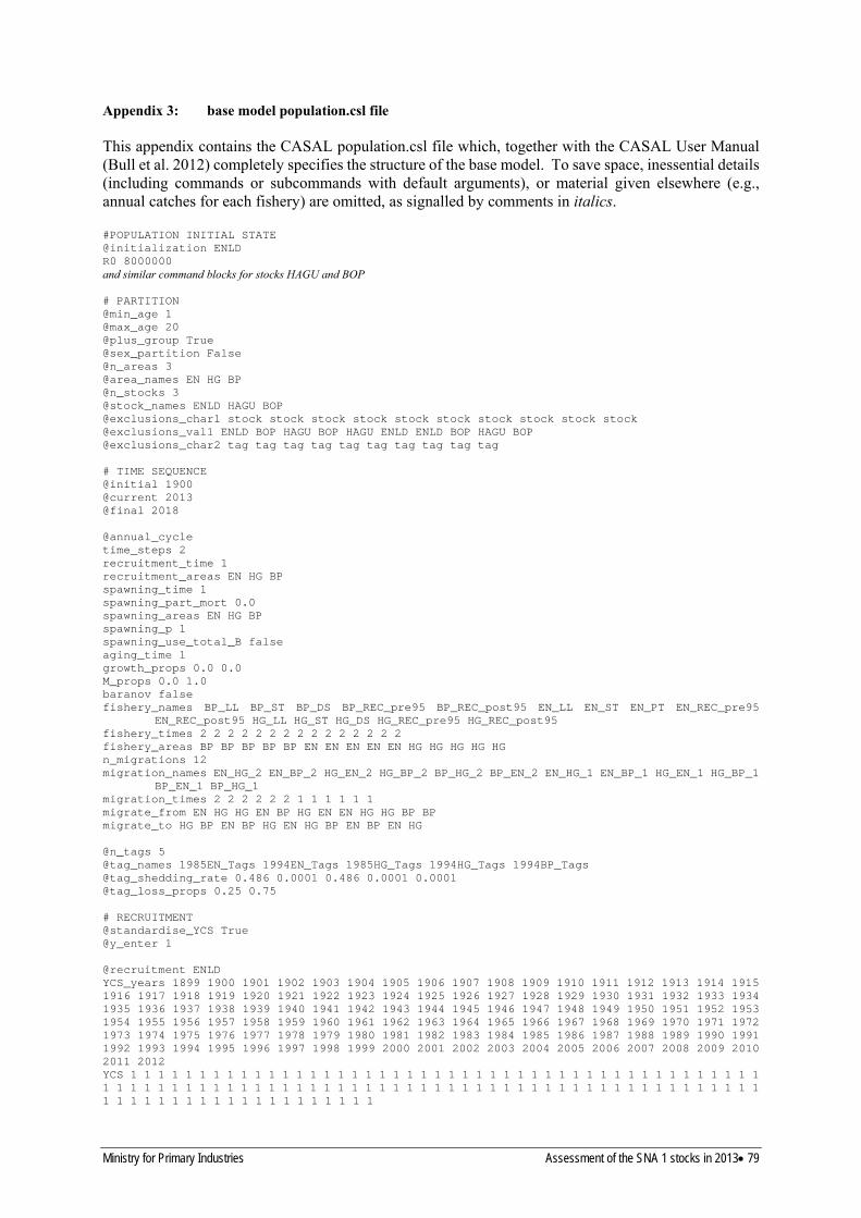
Appendix 3: base model population.csl file

This appendix contains the CASAL population.csl file which, together with the CASAL User Manual (Bull et al. 2012) completely specifies the structure of the base model. To save space, inessential details (including commands or subcommands with default arguments), or material given elsewhere (e.g., annual catches for each fishery) are omitted, as signalled by comments in italics.

#POPULATION INITIAL STATE @initialization ENLDR0 8000000 and similar command blocks for stocks HAGU and BOP

# PARTITION @min_age 1@max_age 20@plus_group True@sex_partition False@n_areas 3@area_names EN HG BP@n_stocks 3@stock_names ENLD HAGU BOP@exclusions_char1 stock stock stock stock stock stock stock stock stock stock@exclusions_val1 ENLD BOP HAGU BOP HAGU ENLD ENLD BOP HAGU BOP@exclusions_char2 tag tag tag tag tag tag tag tag tag tag

# TIME SEQUENCE@initial 1900@current 2013@final 2018

@annual_cycletime_steps 2recruitment_time 1 recruitment_areas EN HG BP spawning_time 1spawning_part_mort 0.0spawning_areas EN HG BPspawning_p 1spawning_use_total_B falseaging_time 1growth_props 0.0 0.0M_props 0.0 1.0baranov false fishery_names BP_LL BP_ST BP_DS BP_REC_pre95 BP_REC_post95 EN_LL EN_ST EN_PT EN_REC_pre95

EN_REC_post95 HG_LL HG_ST HG_DS HG_REC_pre95 HG_REC_post95fishery_times 2 2 2 2 2 2 2 2 2 2 2 2 2 2 2fishery_areas BP BP BP BP BP EN EN EN EN EN HG HG HG HG HGn_migrations 12migration_names EN_HG_2 EN_BP_2 HG_EN_2 HG_BP_2 BP_HG_2 BP_EN_2 EN_HG_1 EN_BP_1 HG_EN_1 HG_BP_1

BP_EN_1 BP_HG_1 migration_times 2 2 2 2 2 2 1 1 1 1 1 1migrate_from EN HG HG EN BP HG EN EN HG HG BP BPmigrate_to HG BP EN BP HG EN HG BP EN BP EN HG

@n_tags 5@tag_names 1985EN_Tags 1994EN_Tags 1985HG_Tags 1994HG_Tags 1994BP_Tags@tag_shedding_rate 0.486 0.0001 0.486 0.0001 0.0001@tag_loss_props 0.25 0.75

# RECRUITMENT @standardise_YCS True@y_enter 1

@recruitment ENLDYCS_years 1899 1900 1901 1902 1903 1904 1905 1906 1907 1908 1909 1910 1911 1912 1913 1914 19151916 1917 1918 1919 1920 1921 1922 1923 1924 1925 1926 1927 1928 1929 1930 1931 1932 1933 1934 1935 1936 1937 1938 1939 1940 1941 1942 1943 1944 1945 1946 1947 1948 1949 1950 1951 1952 1953 1954 1955 1956 1957 1958 1959 1960 1961 1962 1963 1964 1965 1966 1967 1968 1969 1970 1971 1972 1973 1974 1975 1976 1977 1978 1979 1980 1981 1982 1983 1984 1985 1986 1987 1988 1989 1990 1991 1992 1993 1994 1995 1996 1997 1998 1999 2000 2001 2002 2003 2004 2005 2006 2007 2008 2009 2010 2011 2012 YCS 1 1 1 1 1 1 1 1 1 1 1 1 1 1 1 1 1 1 1 1 1 1 1 1 1 1 1 1 1 1 1 1 1 1 1 1 1 1 1 1 1 1 1 1 1 1 1 1 1 1 1 1 1 1 1 1 1 1 1 1 1 1 1 1 1 1 1 1 1 1 1 1 1 1 1 1 1 1 1 1 1 1 1 1 1 1 1 1 1 1 1 1 1 1 1 1 1 1 1 1 1 1 1 1 1 1 1 1 1 1 1 1 1 1


n_rinitial 0 SR BH steepness 0.85first_free 1966 last_free 2007 year_range 1995 2004and similar command blocks for HAGU and BOP, with the following differences: first_free was 1951 for HAGU and 1971 for BOP

@randomisation_method empirical@first_random_year 2008

#SIZE WEIGHT @size_weighta 4.467e-08 b 2.793

# GROWTH {SIZE AT AGE}@size_at_age_type data@size_at_age_step 1@size_at_age_dist lognormal@size_at_age_years 1989 1990 1991 1992 1993 1994 1995 1996 1997 1998 1999 2000 2001 2002 20032004 2005 2006 2007 2008 2009 2010 2011 @size_at_age_miss interpfollowed by one @size_at_age command block for each stock giving the mean sizes at age for each year as shown in Figure 4

#MATURITY AND NATURAL MORTALITY @maturity_propsall allvalues_bounded 3 8 0.00 0.5 1.00 1.00 1.00 1.00 @natural_mortalityall 0.075

# MIGRATION @migration EN_HG_2stock ENLD migrators allprop 0.078and similar command blocks for each of the 11 other migrations; for those occurring at step 1, the subcommand prop always had value 1

# FISHING MORTALITY @fishery EN_LLyears 1900 1901 … 2013catches 233 311 … 707 future_years 2014 2015 2016 2017 2018future_catches 707 707 707 707 707 selectivity Sel_LLU_max 0.7 followed by a similar command block for each of the other 19 fisheries defined above, with historic catches as given in Appendix 2 and future catches (at 2013 levels for commercial and as an exploitation rate for recreational (refer Section 4.8))

#TAGGING DETAILS @tag 1985EN_Tagstag_name 1985EN_Tagsarea EN stock ENLD release_type deterministicyear 1985step 1mature_only Falsenumber 6782 plus_group Falseclass_mins 20 21 … 80 81 props_all 0.000236586 0.000106942 … 0.000276229 0mortality 0.0followed by a similar command block for each of the other four tag release episodes

#SELECTIVITIES @selectivity_names Tot-pop Sel_LL Sel_ST Sel_PT Sel_DS Sel_OTHER Sel_REC_pre95 Sel_REC_post95Sel_UNIFORM Tag-bio_sel Sel_RES Sel_lf15 ssb-bio

@selectivity Sel_LLall double_normal 7.809513 1.861128 100 @selectivity Sel_STall double_normal 5.155023 0.835889 17.21431 @selectivity Sel_DSall double_normal 6.648807 1.35788 34.94152 @selectivity Sel_RESall double_normal 4.543643 2.346748 2.55016


@selectivity Sel_REC_pre95all double_normal 4.550965 0.5 10.24395 @selectivity Sel_REC_post95all double_normal 5.29985 0.500005 10.39953 @selectivity Sel_VBall double_normal 2.000000 0.810831 100 @selectivity Sel_PTall double_normal 6 1.5 30 @selectivity Sel_OTHERall double_normal 7 2 6.5 @selectivity Sel_UNIFORMall constant 1 @selectivity Tag-bio_selall size_based knife_edge 25@selectivity Sel_lf15all size_based knife_edge 15@selectivity Tot-popall size_based knife_edge 5@selectivity ssb-bioall knife_edge 4


Appendix 4: Relative and absolute abundance model input values. Assumed base model CVs are given in brackets.

Year BP_Tag_bio BP_Btcpue BP_Llcpue EN_Llcpue HG_Llcpue HG_Res_abund

1983 6000 (0.4) – – – – 8 150 580 (0.25)

1985 – – – – – 11 197 900 (0.31)

1986 – – – – – 6 751 430 (0.32)

1987 – – – – – 13 300 900 (0.39)

1988 – – – – – 16 899 000 (0.2)

1989 – – – – – 11 102 600 (0.22)

1990 – – 0.93 (0.15) 0.98 (0.15) 0.79 (0.15) 22 093 300 (0.31)

1991 – – 0.75 (0.15) 0.89 (0.15) 0.78 (0.15) 25 976 000 (0.26)

1992 – – 0.62 (0.15) 0.84 (0.15) 0.88 (0.15) –

1993 – – 0.75 (0.15) 0.96 (0.15) 0.79 (0.15) 10 011 900 (0.18)

1994 – – 0.74 (0.15) 0.98 (0.15) 0.70 (0.15) 19 437 200 (0.15)

1995 – – 0.88 (0.15) 1.01 (0.15) 0.70 (0.15) 11 360 600 (0.15)

1996 – 0.89 (0.15) 0.89 (0.15) 1.18 (0.15) 0.79 (0.15) –

1997 – 1.00 (0.15) 0.97 (0.15) 1.26 (0.15) 0.94 (0.15) –

1998 – 0.90 (0.15) 0.96 (0.15) 0.99 (0.15) 1.08 (0.15) 20 586 000 (0.18)

1999 – 0.94 (0.15) 1.05 (0.15) 1.04 (0.15) 1.16 (0.15) –

2000 – 0.94 (0.15) 0.98 (0.15) 1.01 (0.15) 1.05 (0.15) –

2001 – 0.94 (0.15) 1.02 (0.15) 0.92 (0.15) 1.01 (0.15) 20 866 200 (0.29)

2002 – 1.00 (0.15) 1.05 (0.15) 0.81 (0.15) 1.05 (0.15) –

2003 – 1.09 (0.15) 1.08 (0.15) 0.76 (0.15) 1.10 (0.15) –

2004 – 0.94 (0.15) 1.03 (0.15) 0.87 (0.15) 1.06 (0.15) –

2005 – 1.01 (0.15) 1.06 (0.15) 0.94 (0.15) 0.99 (0.15) –

2006 – 1.06 (0.15) 1.16 (0.15) 0.96 (0.15) 1.14 (0.15) –

2007 – 1.07 (0.15) 1.13 (0.15) 1.06 (0.15) 1.13 (0.15) –

2008 – 1.23 (0.15) 1.27 (0.15) 1.20 (0.15) 1.25 (0.15) –

2009 – 1.01 (0.15) 1.32 (0.15) 1.21 (0.15) 1.20 (0.15) –

2010 – 0.94 (0.15) 1.34 (0.15) 0.96 (0.15) 1.27 (0.15) –

2011 – 1.00 (0.15) 1.26 (0.15) 1.15 (0.15) 1.30 (0.15) –

2012 – 1.11 (0.15) 1.19 (0.15) 1.24 (0.15) 1.24 (0.15) –


assessment of the sna 1 stocks in 2013

Documents